THE MEGAMASER COSMOLOGY PROJECT: GEOMETRIC DISTANCES TOMEGAMASER GALAXIES AND ACCURATE MASSES OF SUPERMASSIVE

BLACK HOLES AT THEIR CENTERS

Cheng-Yu KuoCharlottesville, Virginia

B.S., Physics, National Taiwan University, 2000M.S., Astronomy, University of Virginia, 2007

A Dissertation Presented to the Graduate Facultyof the University of Virginia in Candidacy for the Degree of

Doctor of Philosophy

Department of Astronomy

University of VirginiaAugust, 2011

James A. Braatz

Fred K. Y. Lo

Mark Whittle

Phil Arras

E. Craig Dukes

Mark J. Reid

ii

Abstract

To constrain models of dark energy, the best complement to observations of the

Cosmic Microwave Background is a precise measurement of the Hubble constant. The

H2O megamaser method can measure direct angular-diameter distances to galaxies

in the Hubble flow, and thereby provides an opportunity to determine the Hubble

constant independent of the Extragalactic Distance Ladder. In this thesis we present

sensitive VLBI and single-dish observations of the megamasers in NGC 6264 and

NGC 6323 and measure their distances using the megamaser method. This is the

first time the method has been applied to galaxies beyond 100 Mpc. For NGC 6264

we developed an ensemble approach that fits the systemic masers with a multi-ring

model, and we determine a distance of 150.5±33.6 Mpc (22% accuracy). We also

apply a Bayesian technique that models the maser distribution as a warped disk

and allows for eccentric orbits, and obtain a distance of 152.3±16.2 Mpc (10.6%).

The corresponding H0 is 65.8±7.2 km s−1 Mpc−1. The best fit model from the

Bayesian technique has a slight warp and a small eccentricity (e ∼ 0.06), but this

substructure has only a minor effect on the distance determination. For NGC 6323,

although we made the most sensitive maser map ever observed, we do not obtain a

comparably precise distance measurement because of the extremely low flux densities

of the systemic masers. Nonetheless, the work on this galaxy helped develop a new

self-calibration technique that enables efficient imaging of distant megamaser disks.

In addition to the observations of these two galaxies, we also present sensitive VLBI

images of four other megamaser galaxies, plus a seventh previously published, from

which we determine accurate masses of the supermassive BHs at their nuclei. The

BH masses are all within a factor of 3 of 2.2 × 107M⊙ and the accuracy of each is

primarily limited by the uncertainty in the Hubble constant. These accurate BH

iii

masses contribute to the observational basis for testing the M − σ⋆ relation at the

low-mass end.

iv

Acknowledgements

I feel deeply grateful to the University of Virginia for providing the wonderful learning

environment and abundant resources. The learning and life experiences here are

unforgetable and had a profound impact on my thoughts, life, and mind. With all

the great people and environment in Charlottesville, I think I have had significant

growths in many aspect of my life, including science and spirituality, in the past six

years. These six years have been my richest and happiest time in my life.

I first want to thank all the faculty members and my fellow graduate students in

the astronomy department. The warm atmosphere in the department let me feel that

the astronomy department is just like a big family, even though I am an international

student coming from a different country. I often viewed my fellow graduate students

just as my brothers and sisters, especially those who are close in entrance years. I

learned greatly from them and I will never forget their warmness and kindness.

In the aspect of scientific research, I thank Dr. Fred Lo greatly for introducing me

to work on the Megamaser Cosmology Project (MCP). Although this project is quite

challenging to me, this is the best scientific project I have ever worked on so far. The

richness and depths of this project have trained me to become a real scientist who can

start to do independent research with all the great tools and knowledge learned from

this project. I couldn’t benefit so much without all the great scientists in the MCP

team and at the NRAO, including my primary advisor Jim Braatz, Dr. Fred Lo, Jim

Condon, Mark Reid, Christian Henkel, Violetta Impellizzeri, and Edward Fomalont.

I want to thank my primary advisor Jim Braatz for his kindness and openness in the

past few years in addition to teaching me many things in this project. Although my

ideas were not always right, Jim always allowed me to explore my own ideas with

great freedom. I benefit a lot from this open attitude because as a student who in

v

the past mostly followed the traditional eastern education system, which emphasizes

too much on getting the standard answers and doing well in the exams, there were

few chances we can learn to think out of box and explore/express our own ideas. It

is the training in the MCP that help me enhance my creativity and taught me what

good science really is.

I thank Mark Reid for providing two essntial programs for this project and my

thesis work. Without his powerful programs, I wouldn’t be able to make reliable mea-

surements and modeling needed for the distance determinations for the two primary

galaxies in this thesis. In addition, I learned many important things and techniques

by using his programs. I thank Jim Condon for his great contributions and help to my

thesis work. His encyclopedia-like knowledge in radio astronomy and deep insights

have not only benefit myself, but also benefit all people in the MCP team. I also

thank Christian Henkel for his frequent help for assisting our VLBI observations from

the Effelsberg site.

My Chinese friends have been an important part of my life in the past six years.

While there is still political tension and a gap between Taiwan and the Mainland

China, I have made many good Chinese friends at UVa. These friendships not only

help shorten the gap between both sides of the Taiwan straight, we also develop deep

mutual respect and appreciation, and learn greatly from each other. I thank all of

my dear Chinese friends here.

I thank deeply my parents for sending me to study in the US. While numerous

families in Taiwan do not have sufficient economic power to send their children to

study abroad and their children need to stay close to take care of their families and

parents, my parents have kept themselves so healthy and have been working so hard

(364 days per year) that I can concentrate on my study at UVa without any worry

vi

about their health and the economy of the family.

Finally, I need to thank immensely my primary Buddhist teachers Master Shinyin

and my root guru His Holiness the 14th Dalai Lama Tenzin Gyatso. I thank Master

Shinyin’s great compassion and encouragement to me to study in US. Coming to the

US has greatly opened my world view and allowed me to encounter the most important

figure in my life, His Holiness the 14th Dalai Lama Tenzin Gyatso. His Holiness’s

teachings not only significantly help increase the degree of peace and compassion in

my mind, His interests and insights in science also help me rid of conflicts between

science and spirituality, both of which are critical parts of my life. This enables me to

study both side by side, and use the knowledge and techniques from both disciplines

to help each other. The only way I can reply the kindness of my glorious spiritual

teachers is to continue to cultivate wisdom and compassion, and to help the sentient

beings in the world as much as I can as a simple scientist.

vii

Table of contents

Abstract ii

Acknowledgements iv

List of Figures xiv

List of Tables xv

1 Introduction and Overview of the Megamaser Cosmology Project 11.1 Scientific Background: Dark Energy and its Relationship to the Hubble

Constant . . . . . . . . . . . . . . . . . . . . . . . . . . . . . . . . . . 31.1.1 Introduction to dark energy . . . . . . . . . . . . . . . . . . . 31.1.2 How to constrain the equation of state of DE . . . . . . . . . 7

1.2 Current Status of Hubble Constant . . . . . . . . . . . . . . . . . . . 121.3 Direct Angular Diameter Distance Measurement with the H2O Mega-

maser Method . . . . . . . . . . . . . . . . . . . . . . . . . . . . . . . 151.4 Strategy of the MCP . . . . . . . . . . . . . . . . . . . . . . . . . . . 211.5 Thesis Overview . . . . . . . . . . . . . . . . . . . . . . . . . . . . . . 22

2 The Survey, Sample, Imaging, and Data Reduction 232.1 Qualified Maser Disks for the MCP . . . . . . . . . . . . . . . . . . . 232.2 The Megamaser Disk Sample . . . . . . . . . . . . . . . . . . . . . . 252.3 VLBI Observations . . . . . . . . . . . . . . . . . . . . . . . . . . . . 282.4 VLBI Data Reduction . . . . . . . . . . . . . . . . . . . . . . . . . . 302.5 Relativistic Velocity Assignment . . . . . . . . . . . . . . . . . . . . . 33

3 BH mass measurement and the MBH-σ relation 373.1 Current Status and Methods for BH Mass Determination . . . . . . . 383.2 Results . . . . . . . . . . . . . . . . . . . . . . . . . . . . . . . . . . . 43

3.2.1 VLBI Images, Rotation Curves, and BH Masses . . . . . . . . 433.2.2 The Error Budget For the BH Mass . . . . . . . . . . . . . . . 453.2.3 Notes On Individual Galaxies . . . . . . . . . . . . . . . . . . 483.2.4 Search For Continuum Emission . . . . . . . . . . . . . . . . . 56

viii

3.3 A Supermassive Black Hole or a Central Cluster of Stars or StellarRemnants ? . . . . . . . . . . . . . . . . . . . . . . . . . . . . . . . . 56

3.4 Comparison With Virial BH Mass Estimates . . . . . . . . . . . . . . 623.5 Maser BH masses and the M − σ⋆ relation . . . . . . . . . . . . . . . 643.6 Summary . . . . . . . . . . . . . . . . . . . . . . . . . . . . . . . . . 65

4 The Acceleration Measurement for H2O megamasers in NGC 6264and NGC 6323 674.1 Methods of Acceleration Measurement . . . . . . . . . . . . . . . . . 67

4.1.1 The Eye-balling Method . . . . . . . . . . . . . . . . . . . . . 684.1.2 The GLOFIT Method . . . . . . . . . . . . . . . . . . . . . . 70

4.2 Acceleration Measurement for NGC 6264 . . . . . . . . . . . . . . . . 804.2.1 High Velocity Masers . . . . . . . . . . . . . . . . . . . . . . . 814.2.2 Systemic Masers . . . . . . . . . . . . . . . . . . . . . . . . . 83

4.3 Acceleration Measurement for NGC 6323 . . . . . . . . . . . . . . . . 904.3.1 High Velocity Masers . . . . . . . . . . . . . . . . . . . . . . . 904.3.2 Systemic Masers . . . . . . . . . . . . . . . . . . . . . . . . . 92

5 The Determination of the Angular-Diameter Distance for NGC 6264and NGC 6323 1045.1 Method 1: Ensemble Fitting . . . . . . . . . . . . . . . . . . . . . . . 107

5.1.1 The Method . . . . . . . . . . . . . . . . . . . . . . . . . . . . 1075.1.2 Distance to NGC 6264 . . . . . . . . . . . . . . . . . . . . . . 1095.1.3 Distance to NGC 6323 . . . . . . . . . . . . . . . . . . . . . . 112

5.2 Method 2: Bayesian Fitting . . . . . . . . . . . . . . . . . . . . . . . 1145.2.1 Distance to NGC 6264 with the Circular Orbit Assumption . . 1175.2.2 Distance to NGC 6264 by Allowing Eccentric Orbits . . . . . 119

5.3 Systematic errors . . . . . . . . . . . . . . . . . . . . . . . . . . . . . 1225.3.1 Non-gravitational Acceleration . . . . . . . . . . . . . . . . . . 1235.3.2 Disk Warping . . . . . . . . . . . . . . . . . . . . . . . . . . . 1235.3.3 Radiation Pressure . . . . . . . . . . . . . . . . . . . . . . . . 1245.3.4 H2O Masers as a Wave Phenomenon . . . . . . . . . . . . . . 124

6 Conclusion 1266.1 The Contributions to the Methodology of the MCP . . . . . . . . . . 1266.2 Summary of the Main Scientific Results . . . . . . . . . . . . . . . . . 1296.3 Applying The Virial Estimation Method to Megamaser Galaxies . 132

ix

List of Figures

1.1 The top plot shows the CMB anisotropy power spectrum. These fea-tures seen in the spectrum are the results of the imprint of acousticwaves in the photon-baryon fluid when they are frozen at the epochof recombination. The bottom plot shows the distance D∗ to the lastscattering surface of the CMB, which can be fully determined with theinformation in the power spectrum. . . . . . . . . . . . . . . . . . . 9

1.2 WMAP 1 σ and 2 σ (the inner and outer dotted lines) likelihood sur-faces for w vs. Ωm given priors on H0. The solid lines show the im-provements given by independent values of H0=72 km s−1 Mpc−1 (top)and H0=62 km s−1 Mpc−1 (bottom) with 10% (left) and 3% (right)errors. . . . . . . . . . . . . . . . . . . . . . . . . . . . . . . . . . . . 11

1.3 A model to illustrate how we determine the distance a galaxy with aH2O maser disk . . . . . . . . . . . . . . . . . . . . . . . . . . . . . . 16

1.4 . . . . . . . . . . . . . . . . . . . . . . . . . . . . . . . . . . . . . . . 171.5 The top-left plot shows an H2O maser spectrum of UGC 3789, with the

spectrum for the systemic masers at the bottom. In the middle panelwe plot the velocities of the systemic maser lines as a function of time.The slopes of the fitted straight lines (the solid lines) directly give theaccelerations of the masers. In the right panel, we fit a part of thesystemic maser spectrum with a program (Reid, M.; private commu-nication) that fits multiple lines at multiple epochs simultaneously inorder to remove the systematic effects of line blending and variability.Illustrations and figures are from Braatz et al. (2010). . . . . . . . . . 20

3.1 Characteristic H2O maser spectra. The x-axis shows LSR velocitiesbased on the optical definition. Flux densities of masers can varysignificantly, so the spectra shown here are just representative for par-ticular epochs: January 13 2008 for NGC 1194; February 21 2009 forNGC 2273; April 2 2009 for NGC 2960 (Mrk 1419); November 30 2005for NGC 4388; March 31 2009 for NGC 6264; and April 6 2000 forNGC 6323. . . . . . . . . . . . . . . . . . . . . . . . . . . . . . . . . 50

x

3.2 VLBI maps for the seven 22 GHz H2O masers megamasers analyzed.The maps are color-coded to indicate redshifted, blueshifted, and sys-temic masers, where the “systemic” masers refer to the maser compo-nents having recessional velocities close to the systemic velocity of thegalaxy. Except NGC 4388, maser distributions are plotted relative tothe average position of the systemic masers. For NGC 4388, in whichthe systemic masers are not detected, we plot the maser distributionrelative to the dynamical center determined by fitting the high velocityfeatures with a Keplerian rotation curve. . . . . . . . . . . . . . . . . 51

3.3 Maser distributions (top panels) and rotation curves (bottom panels)for NGC 1194 , NGC 2273, UGC 3789, and NGC 2960. The maserdistribution has been rotated to horizontal to show the scatter in themaser positions and the offset of the systemic masers from the planedefined by high-velocity masers more clearly. The coordinate system ischosen to place the centroid of the high-velocity maser disk (blue andred points) at θy = 0 and the centroid of the systemic masers (greenpoints) at θx = 0. The axes for the maps show relative position in mil-liarcseconds, and North (N) and East (E) are indicated by directionalarrows on each map. The bottom panel for each galaxy shows therotation curves of the redshifted and blueshifted masers (red and bluepoints on the curves) plotted with the best-fit Keplerian (solid curve)and Plummer (dotted curve) rotation curves. The velocities shown inthe figure are the LSR velocities after the special and general relativis-tic corrections. The residuals (data minus Keplerian curve in red andblue; data minus Plummer curve in black) are in the bottom part ofeach figure. Note that we plot the rotation curve with the impact pa-rameter θ (mas) as the ordinate and rotation speed |v| (km s−1) as theabscissa for the convenience of fitting. . . . . . . . . . . . . . . . . . . 52

3.4 Maser distributions (Top panel) and rotation curves (Bottom panel)for NGC 4388 , NGC 6264, and NGC 6323. Please refer to the captionof Figure 3.3 for the description of this figure. . . . . . . . . . . . . . 53

xi

4.1 The left two plots (Fig. 4.1a) show the synthetic spectra that havesimilar flux density distribution, SNR, linewidth, time variation, andacceleration as the dominant maser clump in NGC 6264. A spectrum isgenerated once a month over two years. Therefore, we have 24 epochsof spectra in total. The top-left plot shows the spectra for epochs 0,2, 4, 6, and 8 (black, purple, blue, green, orange, and red) and thebottom-left plot shows the spectra for epochs 10, 12, 14, 16, and 18(black, purple, blue, green, orange, and red). One can see clearly thewhole spectral pattern drifts toward higher velocity with time. Theplot on the right (Fig. 4.1b) shows the best-fit accelerations from theeye-balling method plotted on top of the radial velocities of maserpeaks as a function of time. . . . . . . . . . . . . . . . . . . . . . . . 70

4.2 These six panels show the result of the global fitting for the syntheticspectra (described in section 4.1.1) from epochs 12, 14, 16, 18, 20, and22. The black and blue curves represent the data and fitted model,respectively. The purple curves show the residuals of the fitting. . . 72

4.3 In Fig. 4.3a (the left panel) we compare the fitted peak velocities andaccelerations of the model maser lines with the expected values. Thex and y coordinates of the crosses show the expected values for the ac-celerations and velocities at the reference epoch (epoch 18). The datapoints that show error bars are the measurements from the GLOFITprogram.; Fig. 4.3b (the right panel) shows the peaks of the syn-thetic maser spectra (the plus symbols) as a function of time. The linesegments plotted on top of it correspond to the accelerations measuredfrom the GLOFIT program. The offsets between the line segments andthe average trends of the plus symbols are the result of line blending. 73

4.4 In Fig. 4.4a (the left panel) we compare the fitted peak velocitiesand accelerations of the model maser lines with the expected values.The x and y coordinates of the crosses show the expected values for theaccelerations and velocities at the reference epoch (epoch 18). The datapoints that show error bars are the measurements from the modifiedGLOFIT program.; Fig. 4.4b (the right panel) shows the peaks ofthe synthetic maser spectra (the plus symbols) as a function of time.The line segments plotted on top of it correspond to the accelerationsmeasured from the modified GLOFIT program. . . . . . . . . . . . . 75

4.5 The σ per DOF (i.e. the square root of χ2) as a function of the fixedvelocities after fitting the synthetic spectra with the modified GLOFITprogram. . . . . . . . . . . . . . . . . . . . . . . . . . . . . . . . . . . 77

4.6 A representative spectrum for NGC 6264. This spectrum was observedon 2010 February 9. . . . . . . . . . . . . . . . . . . . . . . . . . . . 80

xii

4.7 In this figure, we plot the radial velocities of NGC 6264 maser peaks asa function of time (the crosses) along with the fitting results from theeye-balling method (for the high velocity masers) or from the modifiedGLOFIT program (for the systemic masers).The data between Day 0and 200 come from spectra taken in Period A; the data between Day300 to 600 from spectra in Period B; and the data between Day 700 to900 are from spectra in Period C. . . . . . . . . . . . . . . . . . . . . 82

4.8 The upper panel shows the spectra from epoch 0 through 5 (purple,blue, green, yellow, and orange), and the bottom panel shows the spec-tra from epoch 6 through 11 (purple, blue, green, yellow, and orange).The whole velocity ranges of the systemic masers in Period A and B aredivided into 7 clumps for the convenience of acceleration measurement. 84

4.9 An example of the Gaussian decomposition for the acceleration mea-surement. In this example, we fit the masers between 10183.0 and10197.7 km s−1 in the spectra. The panels from top to bottom showthe spectra (lines with black color) from epoch 0 through 5. Each ofthe eight Gaussian components fitted to the data are represented bydifferent colors. The purple curves at the bottom of each panel are theresiduals from the fit. . . . . . . . . . . . . . . . . . . . . . . . . . . . 97

4.10 A representative spectrum for NGC 6323. This spectrum was observedon 2008 May 29. . . . . . . . . . . . . . . . . . . . . . . . . . . . . . 99

4.11 In this figure, we plot the radial velocities of NGC 6323 maser peaks asa function of time (the crosses) along with the fitting results from theeye-balling method (for the high velocity masers) or from the modifiedGLOFIT program (for the systemic masers).The data between Day 0and 400 come from spectra taken in Period A; the data between Day400 to 800 from spectra in Period B; and the data between Day 800 to1200 are from spectra in Period C. . . . . . . . . . . . . . . . . . . . 100

4.12 The upper panel shows the spectra from epochs 0 through 3 (purple,blue, green, and orange), the middle panel shows the representativespectra (epoch 4/purple, 6/blue, 8/green, 10/orange) from epochs 4to 14, and the bottom panel shows the representative spectra (epoch13/purple, 15/blue, 17/green, 19/orange) from epochs 15 through 21.Because of both severe blending and low signal-to-noise, we only man-age to measure the accelerations for masers between epochs 4 and 14.We divide the velocity range of interest into four sections for the con-venience of acceleration measurement. . . . . . . . . . . . . . . . . . . 102

xiii

5.1 The left panel shows the Position-Velocity (P-V) diagram for the maserdisk in NGC 6264. The red, green, and blue colors assigned to themaser spots indicate the redshifted, systemic, and blueshifted masers,respectively. The right panel shows the P-V diagram only for the sys-temic masers. We assign a unique color to maser spots from each ring,with each maser ring having its own acceleration : 1.07 km s−1 yr−1

for purple, 0.74 km s−1 yr−1 for blue, 1.79 km s−1 yr−1 for green, 1.55km s−1 yr−1 for orange, and 4.43 km s−1 yr−1 for red. . . . . . . . . 106

5.2 The left panel shows the rotated maser disk in NGC 6264. The red,green, and blue colors assigned to the maser spots indicate the red-shifted, systemic, and blueshifted masers, respectively. Here, we adoptthe convention that the redshifted masers have positive impact param-eters. The right panel shows the distribution of the systemic masers inthe rotated disk. We assign colors to the systemic masers as in Figure5.1. In the following discussion, we call the ring at which the maserswith purple color reside ring 1. We call ring 2 for the masers with bluecolor, ring 3 for green, ring 4 for orange, and ring 5 for red. . . . . . 110

5.3 In this figure, we plot the results (the solid lines) from ensemble-fittingon the position-velocity diagram of the systemic masers in NGC 6264.The best fit distance to NGC 6264 is 150.8±32.8 Mpc (22% accuracy). 112

5.4 The left panel shows the rotated maser disk in NGC 6323. The red,green, and blue colors assigned to the maser spots indicate the red-shifted, systemic, and blueshifted masers, respectively. Here, we adoptthe convention that the redshifted masers have positive impact param-eters. The right panel shows the distribution of the systemic masersin the rotated disk. The red spots represent the masers with an ac-celeration of 0.53±0.16 km s−1 yr−1, the greens have an accelerationof 1.40±0.16 km s−1 yr−1, the blue has an acceleration of 1.64±0.17km s−1 yr−1, and the purples are the maser spots without reliable ac-celeration measurements. . . . . . . . . . . . . . . . . . . . . . . . . 114

5.5 The left panel shows the P-V diagram of the systemic masers withgood acceleration measurements in the ensemble-fitting for NGC 6323.We only adopt the data from Period B in the fitting because there isno reliable acceleration measurements for the data taken in Period A& C. The right panel shows the P-V diagram of the systemic masersincluding the spots with no reliable acceleration measurements. Weuse the average velocity gradient (Ω = 821.4±239.8 km s−1 yr−1) ofthese masers and their average acceleration (a =1.06 km s−1 yr−1) tomake an zero-th order estimate of the maser distance to NGC 6323. 115

xiv

5.6 The probability distribution of the distance to NGC 6264 from theBayesian fitting program. The x-axis shows the distance in Mpc, andthe y-axis shows the relative probability density of the distance. Thehighest probability occurs at D =154.6 Mpc, and the 68% confidencerange centers at 149.2 Mpc with an uncertainty of 19.8 Mpc. Thenon-Gaussian distribution is the result of the Bayesian analysis with-out imposing a strong Gaussian prior. This shows the power of theBayesian approach to explore the real probability distribution of thedata. . . . . . . . . . . . . . . . . . . . . . . . . . . . . . . . . . . . . 119

5.7 The left panel shows the model maser distribution in NGC 6264 fromthe overhead perspective. The right panel shows the best-fit warp fromthe observer’s perspective with model maser spots plotted on top ofit. We deliberately decrease the disk inclination by ∼5 to show thedegree of disk warping more clearly. . . . . . . . . . . . . . . . . . . 120

5.8 The left panel shows the probability distribution of the eccentricity ofthe maser orbits. For the eccentricity distribution, the highest proba-bility occurs at e =0.06. The 68% confidence range of the distributioncenters at 0.10 with an uncertainty of 0.06. It is interesting to noticethat the probability for the maser orbits to be circular is nearly zero,and the non-vanishing eccentricity may have important implicationsfor how the maser disk formed and evolved with time. The right panelshow the probability distribution for the pericenter azimuth. The dis-tribution peaks at = 15.3, with the 68% confidence range centeringat 75.3 (uncertainty=60.0). . . . . . . . . . . . . . . . . . . . . . . . 122

xv

List of Tables

2.1 The Megamaser Sample . . . . . . . . . . . . . . . . . . . . . . . . . 272.2 Observing Parameters . . . . . . . . . . . . . . . . . . . . . . . . . . 292.3 Sample data for NGC 6264 . . . . . . . . . . . . . . . . . . . . . . . . 34

3.1 The BH Masses and Basic Properties of the Maser Disks . . . . . . . 463.2 Upper limit on Continnum Emission from Megamaser Galaxies . . . . 613.3 Comparison of Maser BH Mass with Mass from Virial Estimation . . 61

4.1 Observing dates and sensitivities for NGC 6264 . . . . . . . . . . . . 954.2 Acceleration Measurements for the High Velocity Masers in NGC 6264 964.3 Acceleration Measurements for the Systemic Masers in NGC 6264 . . 984.4 Observing dates and sensitivities for NGC 6323 . . . . . . . . . . . . 994.5 Acceleration Measurements for the High Velocity Masers in NGC 6323 1014.6 Acceleration Measurements for the Systemic Masers . . . . . . . . . . 103

5.1 The Best Fit Model Parameters for NGC 6264 . . . . . . . . . . . . 118

1

Chapter 1

Introduction and Overview of the

Megamaser Cosmology Project

We are in a golden age of cosmology. After Hubble’s ground-breaking discovery of

the expansion of the Universe, the field of cosmology has advanced extraordinarily

over the past few decades. In addition to important discoveries such as the Cosmic

Microwave Background (CMB) Radiation and large scale structure, observations of

Type Ia supernovae in the late 1990’s led to one of the most exciting and puzzling

discoveries − the acceleration of the Universe (Riess et al 1998; Perlmutter et al.

1999).

Observational cosmology was once thought to be a search for two numbers: the

Hubble constant H0 and the deceleration parameter q0 (Sandage 1970). Of these two,

q0 was considered to be particularly important for distinguishing different models

of the Universe (Sandage et al. 1961). This simple picture of the cosmos changed

dramatically after the cosmic acceleration was discovered, and this discovery opened

a new era of cosmology research. “Dark Energy”, which has negative pressure and

accounts for 73% of the total energy density of the Universe, is currently the best

2

candidate to explain the acceleration of the Universe. Since the cosmic acceleration

was discovered, understanding the nature of dark energy has become one of the most

important problems in modern astronomy and astrophysics.

There have been several very promising methods proposed to explore dark energy

with high accuracy. Some methods use the Type Ia supernovae, the Baryon Acoustic

Oscillation, galaxy clusters, or weak gravitational lensing as tools to probe dark energy

(see Frieman, Turner, Huterer 2008) whereas there are also methods that constrain

the equation-of-state parameter w by measuring an accurate Hubble constant H0. In

the Megamaser Cosmology Project (MCP; Reid et al. 2009a; Braatz et al. 2010),

we take the latter approach and aim to determine the Hubble constant H0 to 3%

accuracy in order to measure w to 10%.

The key to a precise Hubble constant is to measure accurate distances to galaxies

well into the Hubble flow (i.e. ≥ 50 Mpc). The galaxies must be distant to reduce

the contribution of the uncertainty coming from peculiar velocities. While measuring

precise distances to astronomical objects has always been important, direct distance

measurements to galaxies in the Hubble flow has been challenging. In the past only

indirect distance measurements through the Extragalactic Distance Ladder were ob-

tained. Such an approach requires several calibration steps in the distance measure-

ment, and since each step can have its own complexity, the final result from such an

approach may be more susceptible to hidden systematic errors. A recent example is

the different Hubble constants measured by Sandage et al. (2006; H0 = 62.3 ± 5.2

km s−1 Mpc−1) and Freeman et al. (2001; H0 = 72 ± 8 km s−1 Mpc−1).

Among all the approaches to measure precise distances, the megamaser method

pioneered by the study of NGC 4258 (Herrnstein et al. 1999) has proven to be the

most effective to make precise and direct distance measurements to galaxies beyond

3

our Local Group. In the Megamaser Cosmology Project, we bypass the extragalactic

distance ladder and apply the megamaser technique to galaxies in the Hubble flow,

obtaining direct angular-diameter distances without any local calibration. Such an

experiment was not possible in the past because of insufficient sensitivity to detect

H2O megamasers at sufficiently large distances. In the past decade, the advent of the

100-m Green Bank Telescope has made this project possible.

In this thesis, I will present the first results of applying the H2O megamaser

method to two galaxies beyond 100 Mpc and determine the Hubble constant directly

without any local calibration. In addition, I will also present six new, accurate (∼5%)

black hole masses measured from precise rotation curves of sub-parsec megamaser

disks, and discuss their implication for the nature of the famous MBH−σ relation. In

the remainder of this chapter, I will discuss the scientific background for dark energy,

current status of H0 measurements, and the methodology of the MCP.

1.1 Scientific Background: Dark Energy and its

Relationship to the Hubble Constant

1.1.1 Introduction to dark energy

Within the framework of Einstein’s theory of general relativity and assuming that

the matter distribution is homogeneous on large scales, the Universe is expected to

decelerate with time if the Universe is made of photons, dark matter, and baryonic

matter. One can see this point from the Friedmann equations:

( a

a

)

=8πG

3c2ρ − k

c2

a2(1.1)

4

a

a= −4πG

3c2

(

ρ + 3p)

, (1.2)

where a ≡ (1+z)−1 is a scale factor of the Universe, ρ is the total energy density (the

sum of matter, radiation, dark energy), p is the total pressure, and k is the curvature

parameter (k=0 for a flat Universe). Since for photons ρ = 1/3p, and for baryonic

matter and cold dark matter p << ρ, the acceleration a must be negative, according

to Equation 1.2.

To explain the acceleration of the Universe while keeping the homogeneity as-

sumption, the Einstein field equations must be modified. There are in general two

ways to modify the field equations: either change the Einstein tensor on the left-hand

side of the equations, or change the energy-stress tensor on the right-hand side:

Rµν − 1

2gµνR = −8πG

c4T µν , (1.3)

where Rµν is the Ricci curvature tensor, R the scalar curvature, and gµν the metric

tensor (the Einstein tensor Gµν is defined as Rµν − 12gµνR).

Changing the Einstein tensor of the field equations gives a modified theory of

gravity. In this case, cosmic acceleration is a manifestation of new gravitational

physics rather than the effect of a new form of energy or particle. A number of

ideas have been explored along this line (Frieman, Turner, & Huterer 2008), from

models motivated by higher-dimensional theories and string theory (Deffayet 2001;

Dvali, Gabadadze, & Porrati 2000) to phenomenological modification of the Einstein-

Hilbert Lagrangian of general relativity (Carrol et al. 2004; Song, Hu, & Sawicki

2007).

Compared to changing the Einstein tensor, modifying the stress-energy tensor

5

part of the field equations has received much more attention from the astronomical

community. While the physical meaning of the modification term is still obscure (i.e.

the anti-gravity nature), one can easily explain the cosmic acceleration and a number

of cosmological observations (see Frieman, Turner, Huterer 2008) by introducing a

new energy-stress component called “dark energy” on the right-hand side of the field

equations. The defining characteristic of dark energy is that it has an equation-

of-state parameter, w ≡ p/ρ, less than -1/3. Such equation-of-state parameter is

required by the Friedmann equations in order to generate positive acceleration a.

However, the counterintuitive anti-gravity nature of dark energy implied by a negative

equation of state still needs to be further studied in order to understand its physical

meaning in depth.

The two current leading models for dark energy are the vacuum energy and

quintessence. The vacuum energy is the simplest but at the same time most puz-

zling form of dark energy. In the Einstein field equations, it has a simple form on the

right-hand side of the equations:

Rµν − 1

2gµνR =

8πG

c4T µν − Λgµν , (1.4)

where Λ is the cosmological constant first proposed by Einstein. This equation re-

quires the pressure of the dark energy pDE = −ρvac, where ρvac ≡ Λ/8πc4 is the energy

density of the quantum vacuum, and this relation implies that the equation-of-state

parameter w=−1. Quantum vacuum has been a great puzzle for physicists because

the observed value for dark energy is some 120 orders of magnitude lower than that

predicted by quantum field theory. This is probably the worst theoretical prediction

in the history of physics, and has been called the “cosmological constant problem”.

Some ideas, including the “anthropic principle” (Weinberg 1987), have been proposed

6

to explain the low, but non-zero cosmological constant. More detailed discussion on

possible solutions can been found in Frieman, Turner, & Huterer (2008).

Quintessence is another important candidate for dark energy. It literally means

the “fifth element” and is a new scalar field φ in the Universe. For a scalar field

φ with Lagrangian density L = ∂µ∂µφ − V (φ), the stress-energy tensor takes the

form of a perfect fluid (Frieman, Turner, Huterer 2008), with ρ = φ2/2 + V (φ)

and p = φ2/2 − V (φ), where φ2/2 is the kinetic energy and V (φ) is the potential

energy. One of the major differences between quintessence and vacuum energy is that

for various quintessence models the equation-of-state parameter w can take values

between -1 and -1/3. In addition, rather than being constant in time and homogeneous

in space, quintessence can in principle clump in space and its energy density and

equation-of-state parameter can change with time. There have been ideas to adopt

more complicated scalar fields to allow w to be less than -1 by modifying the kinetic

term of the Lagrangian. Such examples include the phantom dark energy model.

No matter whether the cosmic acceleration is best explained by a modified theory

of gravity or vacuum energy/quintessence, it will have deep implications and impact

on our understanding of fundamental physics. Each possibility points us to a deeper

level of reality. In the case of dark energy, one can perhaps appreciate the importance

of understanding its nature best through Steven Weinberg’s remark:

It is difficult for physicists to attack this problem (i.e. the nature of dark energy)

without knowing just what it is that needs to be explained, a cosmological constant or a

dark energy that changes with time as the universe evolves; and for this they must rely

on new observations by astronomers. Until it is solved, the problem of dark energy

will be a roadblock on our path to a comprehensive fundamental physical theory.

7

1.1.2 How to constrain the equation of state of DE

Dark energy affects the Universe in two distinct ways: (1) through the Friedman

equations (Eq. 1.1 & 1.2), it alters the rate of expansion of the Universe, H(z) and;

(2) through the perturbation equation (e.g. Hu 2005), it affects the rate of growth of

large-scale structures:

d2δm

dt2+ 2H(a)

dδ

dt= 4πGρmδm, (1.5)

where δm ≡ δρm/ρm is the density perturbation of non-relativistic matter. Therefore,

to understand the nature of dark energy, one must measure the observables that are

functions of either H(z) ,or δm, or both. In particular, the primary observable for

H(z) is the distance to a cosmological object:

D(z) = c

∫ z

0

dz′

H(z′). (1.6)

Note that the distance here is the comoving distance. The luminosity and angular-

diameter distances can be calculated by dividing and multiplying the comoving dis-

tance by the scale factor a(t) ≡ 1/(1 + z).

Among the four most promising dark energy probes that do not involve the CMB,

the Type Ia supernovae technique and the Baryon Acoustic Oscillation method con-

strain the DE properties mainly through D(z); the technique involving measuring

number density of galaxy clusters is sensitive to both D(z) and δρ(z); and the weak

gravitational lensing method that measures the spatial distribution and time evolu-

tion of dark matter probes DE purely through the growth rate of structure δρ(z).

In the Megamaser Cosmology Project, we aim to constrain the equation-of-state

parameter of DE by measuring the Hubble constant to a few percent accuracy. An

accurate Hubble constant has the power to constrain DE because the angular-diameter

8

distance to the last scattering surface (LSS) of CMB photons, D∗ ≡ a(z∗)D(z∗), is

a function of cosmological parameters including w and H0. By determining D∗ and

the relevant cosmological parameters with the observables from the CMB anisotropy

power spectrum, one can obtain a relationship between w and H0. With this relation,

the determination of the Hubble constant directly leads to a measurement of w. We

explain the details as follows.

The acoustic features in the CMB anisotropy power spectrum (Figure 1.1) provide

standard rulers for dark energy probes (Hu 2005). These features are the imprint of

acoustic waves in the photon-baryon fluid when they were frozen at the epoch of

recombination. The distance that these acoustic waves have traveled since the Big

Bang to the time of recombination, s∗, is the most essential CMB standard ruler for

probing dark energy here, and is the key to making an independent determination of

D∗:

s∗ =

∫ a∗

0

da

a2H(a)cs(a) (1.7)

where cs(a), the speed of the acoustic waves, only depends on the photon-baryon

energy density ratio, and can be well determined by full analysis of the relative am-

plitudes of acoustic peaks in the power spectrum.

The values of s∗ and D∗ are related by the characteristic angular scale of the

acoustic peaks in the power spectrum

lA =πD∗

s∗. (1.8)

Note that one cannot directly infer lA from the multipole space positions of the

acoustic peaks in the power spectrum. Rather, a phase correction (Hu et al. 2001) is

9

needed through the following equation:

lm = lA(m − φm), (1.9)

where m labels the peak number, lm is the position of the m-th peak, and φm is

the phase correction that can be determined with full analysis of the CMB power

spectrum. With the absolute calibration of s∗, the CMB then measures the angular

diameter distance D∗ to the LSS in absolute units. Based on the first year WMAP

result, D∗ is determined to be 13.7±0.4 Gpc (Page et al. 2003).

Fig. 1.1.— The top plot shows the CMB anisotropy power spectrum. These featuresseen in the spectrum are the results of the imprint of acoustic waves in the photon-baryon fluid when they are frozen at the epoch of recombination. The bottom plotshows the distance D∗ to the last scattering surface of the CMB, which can be fullydetermined with the information in the power spectrum.

10

While D∗ can be determined precisely with s∗ and lA, one can also express D∗ as

a function of cosmological parameters based on the standard cosmology1:

D(z∗) =1

(1 + z∗)

∫ z∗

0

cH−10 dz

√

((1 + z)3Ωm + (1 + z)4Ωr + (1 + z)3(1+w)ΩDE

, (1.10)

where Ωm is the matter density, Ωr is the radiation density, and ΩDE is the dark

energy density. For a flat Universe, ΩDE is simply 1 − Ωr − Ωm. In addition, Ωmh2

and Ωrh2 can be measured precisely from analyzing the CMB power spectrum (Page

et al. 2003). So, with these measurable quantities, D(z∗) is now only dependent upon

two unknown parameters, w and H0. Therefore, if one can constrain either of these

two parameters, the other can be known. The better we constrain one parameter,

the better we determine the other. In fact, as pointed out by Hu (2005), among all

observables for probing DE in light of the CMB, w is most sensitive to variations in

H0. Hu (2005) concluded that the single most important complement to the CMB

for measuring the DE equation-of-state parameter w at z∼0.5 is a determination of

the Hubble constant to better than a few percent. This insight forms the fundamental

motivation for the Megamaser Cosmology project.

To see more intuitively how the accuracy of w and our ability to distinguish

among DE models depend on the accuracy of the H0 measurement, we use a figure

from Braatz et al. (2006) for demonstration. In Figure 1.2, we compare w constrained

from two different H0 measurements (H0 = 72 km s−1 from Freedman et al. 2001

and H0=62 km s−1 from Sandage et al. 2006). As shown by the two plots on the

left side of the figure, one cannot confidently distinguish quintessence models from

vacuum energy if the Hubble constant measurement is only accurate to 10%. Both

1The flat geometry and constant w are assumed in the equation here for the purpose of explaininghow to constrain w from a precise H0 in a simpler way. The argument can be generalized to includethe effect of curvature.

11

show results that are consistent with the vacuum energy model. However, if H0 can

be determined to 3% accuracy (say if H0 is 62 km s−1 Mpc−1), as shown by the

two plots on the right, one can rule out the vacuum energy model with a confidence

level > 96%. These plots demonstrate that a precise Hubble constant is crucial to

distinguish among different DE models.

Fig. 1.2.— WMAP 1 σ and 2 σ (the inner and outer dotted lines) likelihood surfacesfor w vs. Ωm given priors on H0. The solid lines show the improvements given byindependent values of H0=72 km s−1 Mpc−1 (top) and H0=62 km s−1 Mpc−1 (bottom)with 10% (left) and 3% (right) errors.

12

1.2 Current Status of Hubble Constant

There has been considerable progress in determining the Hubble constant H0 over

the past two decades. After Hubble’s fundamental discovery of the Hubble law in

1929 (Hubble 1929a), the most important milestone for precise H0 determination was

achieved by Freedman et al. (2001) who calibrated the secondary distance indicators

(e.g. Type 1a supernovae) based on Cepheid Period-Luminosity (PL) relation using

the Hubble Space Telescope (HST). They obtained an H0 of 72±8 km s−1Mpc−1,

the most widely accepted Hubble constant at the start of the Megamaser Cosmology

Project.

The error in H0 from Freedman et al. (2001) is dominated by systematic un-

certainty. The primary sources of systematics consist of (1) the zero-point of the

Cepheid PL relation, which was tied directly to the (independently adopted) distance

to the Large Magellanic Cloud (LMC), the anchoring galaxy for the HST Key project

(Freedman et al. 2001); and (2) the differential metallicity corrections to the PL zero

point in going from the relatively low-metallicity (LMC) correction to target galax-

ies of different (and often higher) metallicities. Among these two systematics, the

metallicity correction has been the most controversial.

It is known that the colors and magnitudes of Cepheid variables are affected

by the metal abundances in their atmospheres (e.g. Freedman & Madore 2010).

Therefore, their PL relations should be a function of metallicity. However, predicting

the magnitude and the sign of the metallicity effect from a theoretical perspective

has proven to be difficult (see references in Freedman & Madore 2010). Therefore,

the metallicity corrections have usually been made empirically. With a different

way to treat the metallicity effect, Sandage et al. (2006) obtained an H0 of 62±5

km s−1Mpc−1. It was therefore thought by some people that the bulk of the difference

13

in the Hubble constant between Sandage et al. (2006) and Freedman et al. (2001)

comes from different metallicity corrections. However, after detailed analysis by Riess

et al. (2009b), it has been shown that the bulk of the difference between Sandage et

al. and Freedman et al. originates from inaccurate non-geometric distances to the

Galactic Cepheids used in Sandage et al. (2006), their lack of sufficient number of

long-period (P > 30 days) Cepheids in the calibration, and error in the reddening

correction. The error in the metallicity correction contributes less.

The most important progress in improving the systematic uncertainty of H0 in the

past decade has been made through improving the zero-point calibration and bypass-

ing the controversial metallicity correction by basing the calibrations of the Cepheid

PL relations on either new, accurate parallax distances of Galactic Cepheids (Freed-

man & Madore 2010) or Cepheids in the inner field of NGC 4258 (Riess et al. 2009,

2011). This approach not only has a stronger basis for accurate zero-point calibration

of the PL relations, but most importantly it avoids the need for a significant metallic-

ity correction because the Cepheids in the Galaxy and NGC 4258 have a comparable

metal abundance to the galaxies from which the peak absolute magnitude of Type

Ia supernovae is calibrated. The character of the metallicity uncertainty has changed

from being a systematic to a random uncertainty. In addition to the aforementioned

approach, the metallicity effect has been further reduced by measuring Cepheids in

the near-infrared, where the metallicity dependence is diminished (see Riess et al.

2009).

With the new approaches to reduce systematic errors, Freedman & Madore (2010)

give an H0 of 73±5 km s−1Mpc−1, and Riess et al (2009) & (2011) give an H0 of 74±4

km s−1Mpc−1 and 74±2 km s−1Mpc−1, respectively. These new H0 measurements lead

to a new constraint on the equation-of-state parameter of dark energy with ∼10%

14

accuracy. The authors aim to improve H0 to 1-2% accuracy in the coming decades

with more accurate parallax distances of Galactic Cepheids from GAIA (and perhaps

SIM) for accurate zero-point calibration of the PL relations, and with observations

of Cepheids at mid-IR with JWST to reduce the metallicity effect and scatter in the

PL relations. While these authors have claimed obtaining a percentage level Hubble

constant, we have to caution the reader that part of the calibrations in Riess et al.

(2009) and (2011) are based on an assumed 3% maser distance to NGC 4258. One

should note that a 3% distance to NGC 4258 has not yet been achieved by any group,

and the 3% is just the anticipated goal with all the new observations on NGC 4258

(Argon et al. 2007; Humphreys et al 2008), which are still being analyzed (Ried;

private communication). Therefore, the actual uncertainties from the work of Riess

et al. should actually be higher than what they have claimed.

While there has been significant improvement in the Hubble constant measure-

ment in the optical, given the complexity and multiple steps involved in the calibra-

tion process, there could be still hidden systematic errors. Therefore, an independent

measurement of the Hubble constant without appealing to the Extragalactic Distance

Ladder would be highly valuable. The most promising approach that can measure H0

without the need to resort to other cosmological parameters is the H2O Megamaser

technique (e.g. Herrnstein et al. 1999; Braatz et al. 2010). With precise astrometry

observations with VLBI, the H2O Megamaser technique can potentially be used to

measure distances to galaxies out to ∼200 Mpc. Since these galaxies are already in

the Hubble flow, a direct measurement of H0 with megamaser galaxies can be done

without the Extragalactic Distance Ladder and any local calibration. Such a mea-

surement would be unprecedented. Finally, even when the maser galaxies are too

close to be in the Hubble flow, more accurate maser distances to these galaxies can

15

also be used as the anchors for calibrating the Extragalactic Distance Ladder and

be used to check the accuracy of the previous calibrations based on Cepheids in the

LMC, Milky Way and NGC 4258.

1.3 Direct Angular Diameter Distance Measure-

ment with the H2O Megamaser Method

The H2O megamaser method involves sub-milliarcsecond resolution imaging and

single-dish monitoring of H2O maser emission from sub-parsec circumnuclear disks

at the center of active galaxies, a technique first established by the study of NGC

4258 with VLBI (Herrnstein et al. 1999). In this technique, one determines the

distance to a maser galaxy by measuring four orbital parameters (i.e. the radius,

velocity, acceleration, and inclination of an orbit) with precise maser positions, ve-

locities, and accelerations. Here, we use the example of NGC 4258 (Herrnstein et al.

1999), UGC 3789 (Braatz et al. 2010) and a cartoon plot to explain the principle

behind this technique.

Figure 1.3 shows a cartoon plot of masing gas orbiting around a supermassive

black hole in a circular orbit at the center of a galaxy. D is the distance from the

observer to the galaxy, r is the physical radius of the orbit, and ∆θ is apparent angular

radius seen by the observer. Based on simple geometry, we can express the distance

as

D =r

∆θ. (1.11)

According to Newton’s second law, the gravitational acceleration a of the masing gas

16

Fig. 1.3.— A model to illustrate how we determine the distance a galaxy with a H2Omaser disk

in the circular orbit is related to the orbital velocity v0 and physical radius r with

a =v2

0

r. (1.12)

For convenience, the above equation can be re-written as

r =v2

0

a. (1.13)

By combining Equations 1.11 & 1.13, and correcting the maser velocity and acceler-

17

ation for the inclination of the orbit, the distance D can be expressed as

D =v2

0

a ∆θsin i . (1.14)

Therefore, one can determine an accurate distance to a megamaser galaxy if the four

parameters in Equation 1.14 can be determined precisely. Now, let’s use the real data

from NGC 4258 and UGC 3789 to illustrate how to measure these parameters.

Fig. 1.4.—

Figure 1.4 shows the the maser distribution and the position-velocity (PV) dia-

gram of the H2O maser disk at the center of NGC 4258. The black hole is sitting

at the center of the disk with a jet ejected toward the top and bottom side of the

disk. The data points in the VLBI maps and rotation curves are color-coded to in-

dicate redshifted, blueshifted (the redshifted/blueshifted masers are also called “high

18

velocity” masers throughout the thesis), and systemic masers, where the “systemic”

masers refer to the maser spectral components having velocities close to the systemic

velocity of the galaxy. Note that the redshifted and blueshifted masers are located

very close to the mid-line (the intersection of the plane of the sky and the disk) of

the disk and can be traced nearly perfectly with a Keplerian rotation curve in the

PV diagram. The systemic masers are located in front of the black hole2, and in the

PV diagram they can be beautifully fit with a straight line, a feature that indicates

that these masers lie in a single narrow ring in the disk.

As shown in Figure 1.4, the intersection between the straight line and the Kep-

lerian rotation curve that fit the systematic and high velocity masers directly give

the orbital velocity V0 and angular size ∆θ of the ring in which the systemic masers

reside. In addition, with the angular offset y of the systemic masers from the black

hole in the vertical direction, one can obtain the inclination i of the orbit for systemic

masers

i = cos−1(y

∆θ) . (1.15)

Therefore, one can obtain three parameters for the distance measurement from VLBI

observation. The remaining parameter, a, has to be measured from multi-epoch

monitoring of maser spectra. Here, we use UGC 3789 from Braatz et al. (2010) to

illustrate how to measure the centripetal acceleration of H2O masers.

It is believed that the origin of the accelerations of H2O masers that we observe is

the centripetal acceleration due to the gravity of the black hole at the center of maser

disk. That the maser is accelerating does not mean that the masing gas is spiraling

toward the black hole. Rather, they stay in a circular orbit because the acceleration

2The mid-line of the disk and places in front of the black hole are particularly favorable for maseremission because in these locations the path lengths for maser amplification reach maximum values(Lo 2005).

19

due to gravity is balanced by the centrifugal acceleration that keeps the object in

orbit. While the orbital speed remains the same, the centripetal force causes the

masing gas to keep changing directions in order to maintain the circular orbit, and

therefore the line-of-sight velocity seen by the observer will keep changing. The rate

of change in the observed maser velocity is the centripetal acceleration along the line

of sight that we want to measure.

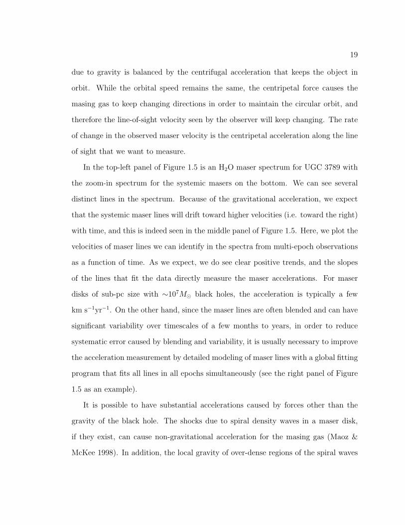
In the top-left panel of Figure 1.5 is an H2O maser spectrum for UGC 3789 with

the zoom-in spectrum for the systemic masers on the bottom. We can see several

distinct lines in the spectrum. Because of the gravitational acceleration, we expect

that the systemic maser lines will drift toward higher velocities (i.e. toward the right)

with time, and this is indeed seen in the middle panel of Figure 1.5. Here, we plot the

velocities of maser lines we can identify in the spectra from multi-epoch observations

as a function of time. As we expect, we do see clear positive trends, and the slopes

of the lines that fit the data directly measure the maser accelerations. For maser

disks of sub-pc size with ∼107M⊙ black holes, the acceleration is typically a few

km s−1yr−1. On the other hand, since the maser lines are often blended and can have

significant variability over timescales of a few months to years, in order to reduce

systematic error caused by blending and variability, it is usually necessary to improve

the acceleration measurement by detailed modeling of maser lines with a global fitting

program that fits all lines in all epochs simultaneously (see the right panel of Figure

1.5 as an example).

It is possible to have substantial accelerations caused by forces other than the

gravity of the black hole. The shocks due to spiral density waves in a maser disk,

if they exist, can cause non-gravitational acceleration for the masing gas (Maoz &

McKee 1998). In addition, the local gravity of over-dense regions of the spiral waves

20

Fig. 1.5.— The top-left plot shows an H2O maser spectrum of UGC 3789, with thespectrum for the systemic masers at the bottom. In the middle panel we plot thevelocities of the systemic maser lines as a function of time. The slopes of the fittedstraight lines (the solid lines) directly give the accelerations of the masers. In theright panel, we fit a part of the systemic maser spectrum with a program (Reid, M.;private communication) that fits multiple lines at multiple epochs simultaneously inorder to remove the systematic effects of line blending and variability. Illustrationsand figures are from Braatz et al. (2010).

can also introduce additional acceleration for masing gas in the disk (Humphreys et al.

2008). If these extra accelerations do exist and are not accounted for in the distance

determination, there will be additional systematic errors. Therefore, one may need

a good theoretical model for the density waves in the maser disk to estimate the

magnitude of the non-gravitational acceleration and understand its impact on the

distance measurement.

21

1.4 Strategy of the MCP

In order to determine the Hubble constant to 3% accuracy, we aim to measure accurate

(i.e. ≤10%) distances to about 10 maser galaxies in the Hubble flow (i.e. ≥50 Mpc).

To achieve this goal, in addition to precise VLBI astrometry for these galaxies, we

also need sensitive large surveys to find more megamaser galaxies similar to NGC

4258. In the MPC, we follow a four step approach:

1. Survey with the Green Bank Telescope (GBT) to identify additional high-

quality disk masers in the Hubble flow for ∼10% distance measurements.

2. Image the sub-pc megamaser disks to obtain their rotation curves with the

High Sensitivity Array (VLBA+GBT+EB)3

3. Measure accelerations of masers accurate to << 10% by monitoring their

spectra over a timescale of a few years.

4. Determine the distance to maser host galaxies by modeling the maser disk

kinematics. Along with the best fit recession velocity of maser galaxies, we use the

maser distance to measure the Hubble constant.

As the MCP continues to discover and image megamaser disks, an important

result, in addition to the distance determination, is the accurate measurement of the

masses of black holes at the centers of these megamaser galaxies. These accurate black

hole masses provide an important basis for testing and understanding the nature of

the famous correlation between black hole mass and stellar velocity dispersion of a

galactic bulge, the MBH−σ relation.

3The VLBA is a facility of the National Radio Astronomy Observatory, which is operated by theAssociated Universities, Inc. under a cooperative agreement with the National Science Foundation(NSF). The Effelsberg 100-m telescope is a facility of the Max-Planck-Institut fur Radioastronomie

22

1.5 Thesis Overview

As a part of the Megamaser Cosmology Project, the observational aspect of this thesis

focuses primarily on the Very Long Baseline Interferometry (VLBI) imaging of the

current best megamaser disks. The surveys were mainly conducted by Braatz et al.

(in prep), Braatz & Gugliucci (2009), and previous work. In Chapter 2, I will first

give a brief summary of the current status of our survey, followed by the presentation

of the sample of maser galaxies, VLBI observations and data reduction. The full

detailed data reduction procedure for the VLBI observations in the MCP will be

presented in the appendix. In Chapter 3, I will show the VLBI results of the current

best seven megamaser disks in MCP, present the analysis of BH masses based on the

VLBI results, investigate the validity of our assumption that we are truly measuring

the masses of black holes and finally discuss the implication of these black hole masses

for the MBH−σ relation.

In Chapter 4, I present the analysis of the acceleration measurements for two of

the maser galaxies (NGC 6323 and NGC 6264) that we target for geometric distances

with the megamaser technique. The actual distance determinations for these two

galaxies will be discussed in Chapter 5, along with the discussion of the possible

systematic uncertainties for the megamaser technique. In Chapter 6, I summarize

the whole thesis.

23

Chapter 2

The Survey, Sample, Imaging, and

Data Reduction

2.1 Qualified Maser Disks for the MCP

Accurate distance measurement with the H2O megamaser technique requires maser

disks to satisfy a few criteria to minimize both statistical and systematic errors: (1)

The system must be rich in bright features at both systemic and high velocities; (2)

The maser lines need to be bright enough (i.e. ≥ 30 mJy) for self-calibration; (3) The

systemic masers should show clear accelerations; and (4) The high velocity features

must obey Keplerian rotation. While the last two requirements are self-evident and

indispensible for distance measurement, the first two points deserve more elaboration.

Rich maser features with high flux densities are critical in many aspects of the

MCP. In the initial stage of the MCP, the peak flux of a maser system usually needs to

be higher than 100 mJy in order to make self-calibration possible. Otherwise, we have

to observe the maser galaxies in phase-referencing mode, and this has proven to be

too inefficient to obtain sufficient sensitivity in a reasonable amount of time. Since it

24

is rare for maser galaxies beyond 50 Mpc to have fluxes higher than 100 mJy, over the

past few years, we have developed a new technique that makes self-calibration feasible

with masers of only ∼ 30 mJy. However, multiple such maser lines are necessary for

applying this new technique (see section 2.4 for a brief description).

High maser flux density is also important for VLBI astrometry and accurate ac-

celeration measurements of masers. The relative position accuracy δθ of a maser spot

(presumably a point source) in the VLBI imaging is

δθ =θbeam

2 SNR, (2.1)

where θbeam is the synthesized beam size and SNR is the signal-to-noise ratio of the

maser spot in the map. Since ∼5 µarcsec position accuracy is usually necessary to

measure distance precisely, the optimal flux density of the systemic masers would

be ≥ 30 mJy for an average beam of 0.5 mas and a 12-hour VLBI observation that

includes the Very Long Baseline Array (VLBA)1, the 100-m Green Bank Telescope

(GBT) and the Effelsberg 100-m telescope2. In addition to the position accuracy

of masers, the precision of acceleration measurements also depends on SNR. While

there are many factors that can affect the accuracy of acceleration measurements (e.g.

blending, variability, time baseline), in general higher SNR is necessary for accurate

acceleration determination. Based on current experience, multiple lines with flux

density > 10 mJy are required for a ≈10% measurement if the acceleration is relatively

high (e.g. 4 km s−1 yr−1). For masers with low accelerations (e.g. < 1 km s−1 yr−1),

flux densities above ∼40 mJy would be needed. For megamaser galaxies well in the

1The VLBA is a facility of the National Radio Astronomy Observatory, which is operated by theAssociated Universities, Inc. under a cooperative agreement with the National Science Foundation(NSF).

2The Effelsberg 100-m telescope is a facility of the Max-Planck-Institut fur Radioastronomie

25

Hubble flow (≥ 70 Mpc), these requirements mean that the maser galaxies needed

for the MCP must be intrinsically brighter than NGC 4258 (Distance = 7.2 Mpc).

Based on how well H2O maser disks satisfy the above requirements, we divide

the discovered maser disks into three classes:(1) “Class A” disks satisfy all these

requirements well and can be used to measure distances; (2) “Class B” disks do not

satisfy the requirements for distance measurement, but have multiple, detectable high

velocity spots that enable measurement of the black hole mass; and (3) “Class C”

disks are currently too faint for either distance or black hole mass measurement, but

are monitored once or twice per year in search of flares that would elevate them to

Class A or B.

In order to find additional maser galaxies for distance and black hole mass mea-

surement, surveys are very important. In this thesis, I will only briefly mention the

result of the surveys. Details of the MCP surveys are forthcoming in Braatz et al.

(2011).

2.2 The Megamaser Disk Sample

In the MCP, we used the 100-m Green Bank Telescope (GBT) to search for H2O

megamasers in narrow-line AGNs, primarily drawn from the Sloan Digital Sky Survey

and the all-sky 2MASS Redshift Survey, plus a smaller number of X-ray selected AGN

and “apparently normal” galaxies (cf. Braatz & Gugliucci 2008). We mainly look for

H2O megamasers in narrow-line AGNs because based on the standard AGN model

these galaxies are more likely to host edge-on accretion disks, which are preferable

for megamasers to occur.

Most megamasers discovered in the past decade were found with the GBT, mainly

by surveys associated with the MCP in which the overall detection rate is ∼3%.

26

Altogether, there are 146 galaxies detected as sources of H2O maser emission3. Most

of the H2O maser emitters originate in AGN (Lo 2005). Based on the post-detection

statistics, about 20% of them show spectra suggestive of emission from sub-parsec

scale, edge-on, circumnuclear disks. The rest of the H2O maser sources among the

146 galaxies are most likely associated with starburst activity in the nuclear regions

of these galaxies.

In the MCP, we have been conducting VLBI observations of four “Class A” mega-

maser disks (UGC 3789, MRK 1419, NGC 6323, and NGC 6264) to determine their

angular diameter distances and black hole masses. The distance measurements for

NGC 6264 and NGC 6323 will be the focus of this thesis. In addition to these Class

A objects, we also have VLBI data on three “Class B” megamaser disks (NGC 4388,

NGC 1194, and NGC 2273) for which we would not determine accurate distances

but can still make precise black hole mass measurements (Chapter 3). Table 2.1 lists

coordinates, recession velocities, spectral types, and morphological types for these

seven galaxies.

3https://safe.nrao.edu/wiki/bin/view/Main/MegamaserCosmologyProject

27

Table 2.1. The Megamaser Sample

R.A. Decl. δRA δDEC Vsys δVsys Spectral HubbleName (J2000) (J2000) (mas) (mas) (km s−1) (km s−1) Type Type

NGC 1194 03:03:49.10864a −01:06:13.4743a 0.2 0.4 4051 15 Sy 1.9 SA0+NGC 2273 06:50:08.65620b 60:50:44.8979b 10h 10h 1832 15 Sy 2 SB(r)aUGC 3789 07:19:30.9490c 59:21:18.3150c 10h 10h 3262 15 Sy 2 (R)SA(r)abNGC 2960 09:40:36.38370d 03:34:37.2915d 10h 10h 4945 15 Liner Sa?NGC 4388 12:25:46.77914e 12:39:43.7516e 0.4 0.3 2527 1 Sy 2 SA(s)bNGC 6264 16:57:16.12780f 27:50:58.5774f 0.3 0.5 10213 15 Sy 2 S ?NGC 6323 17:13:18.03991g 43:46:56.7465g 0.2 0.4 7848 10 Sy 2 Sab

Note. — (1)The systemic (recessional) velocities of the galaxies, Vsys, listed here are based on the “optical” velocityconvention (i.e. no relativistic corrections are made) , measured with respect to the Local Standard of Rest (LSR). ExceptNGC 4388, the systemic velocities Vsys are obtained from fitting a Keplerian rotation curve to the observed data as describedin section 3. The uncertainties δVsys given here include both the fitting error and a conservative estimate of the systematicerror. The fitting error is typically only about 5 km s−1 and the systematic error is from possible deviation of the positionof the BH from (θx, θy) = (0, 0) (see section 3), which is assumed in our rotation curve fitting. For NGC 4388, we adoptthe observed HI velocity from Lu et al. (2003), which has a small but perhaps unrealistic error. (2) The positions ofUGC 3789, NGC 1194, NGC 6323, and NGC 4388 refer to the location of maser emission determined from our VLBI phase-referencing observations. The positions of NGC 2273 and NGC 2960 are determined from K-band VLA A-array observationsof continuum emission from program AB1230 and maser emission from AB1090, respectively. The maser position for NGC6264 is derived from a phase-referencing observation in the VLBA archival data (project BK114A). (3) The Seyfert typesand morphological classifications are from the NASA/IPAC Extragalactic Database (NED).

aThe position of the maser spot at Vop = 4684 kms−1, where Vop is the “optical” velocity of the maser spot relative tothe LSR.

bThe position of the radio continuum emission observed at 21867.7 MHz and 21898.9 MHz.

cThe position of the maser spot at Vop = 2689 kms−1.

dThe position of the maser spot at Vop = 4476 kms−1.

eThe position of the maser spot at Vop = 2892 kms−1.

fThe average position of the masers with velocities from Vop = 10180 kms−1 to Vop = 10214 kms−1

gThe position of the maser spot at Vop = 7861 kms−1.

hFor all positions derived from VLA observations, we use 10mas as the actual position error, rather than the fitted errorsfrom the VLA data, which are only a few mas for these galaxies. The reason is that the systematic error caused by theimperfect tropospheric model of the VLA correlator can be as large as a few to 10s mas. A 10 mas position error usuallyleads to a ≈ 3 − 5 % error in the BH mass for the megamasers presented here. Note that although the position for UGC3789 is derived from a VLBI phase-referencing observation with a phase calibrator 2.1 away, the position of this calibratoris derived from a VLA observation. So, we also use 10 mas as the actual position accuracy for UGC 3789.

28

2.3 VLBI Observations

The megamaser galaxies in our sample were observed between 2005 and 2010 with

the VLBA, augmented by the GBT and in most cases the Effelsberg 100-m telescope.

Table 2.2 shows the basic observing information including experiment code, date

observed, antennas used, and sensitivity.

We observed the megamasers either in a phase-referencing or self-calibration mode.

With phase-referencing we perform rapid switching of the telescope pointing between

the target source and a nearby (< 1) phase calibrator (every ∼ 50 seconds) to correct

phase variations caused by the atmosphere. In a self-calibration observation, we use

the brightest maser line(s) to calibrate the atmospheric phase. In both types of obser-

vations, we placed “geodetic” blocks at the beginning and end of the observations to

solve for atmosphere and clock delay residuals for each antenna (Reid et al. 2009b).

For NGC 6323 and NGC 6264, we also placed a geodetic block in the middle of the

observations to avoid the zenith transit problem at the GBT and to obtain better

calibration. In each geodetic block, we observed 12 to 15 compact radio quasars that

cover a wide range of zenith angles, and we measured the antenna zenith delay resid-

uals to ∼ 1 cm accuracy. These geodetic data were taken in left circular polarization

with eight 16-MHz bands that spanned ∼ 370 - 490 MHz bandwidth centered at a

frequency around 22 GHz; the bands were spaced in a “minimum redundancy” man-

ner to sample, as uniformly as possible, all frequency differences between IF bands in

order to minimize ambiguity in the delay solution (Mioduszewski & Kogan 2009). We

also observed strong compact radio quasars every ∼ 20 minutes to 2 hours in order

to monitor the single-band delays and electronic phase differences among and across

the IF bands. The errors of the single-band delays are < 1 nanosecond.

29

Table 2.2. Observing Parameters

Experiment Synthesized Beam Sensitivity ObservingCode Date Galaxy Antennasa (mas x mas,deg)b (mJy) Modec

BB261d 2005 Mar 06 UGC 3789 VLBA, GB, EB 0.55×0.55, 39.0 1.0 Self-cal.BB242Be 2007 Nov 13 NGC 1194 VLBA, GB 2.45×0.36,−7.5 ∼ 1.5 Self-cal.BB242De 2008 Jan 21 NGC 1194 VLBA, GB 1.83×0.44, −10.5 2.1 Phase-ref.BB261B 2009 Feb 28 NGC 2273 VLBA, GB 0.69×0.39, −22.4 0.5 Self-cal.BB261F 2009 Apr 06 NGC 6264 VLBA, GB, EB 0.93×0.38,−24.8 0.5 Self-cal.BB261H 2009 Apr 18 NGC 6264 VLBA, GB, EB 1.02×0.29,−14.7 0.3 Self-cal.BB261K 2009 Nov 25 NGC 6264 VLBA, GB, EB, VLA 1.10×0.30,−9.7 0.5 Self-cal.BB261Q 2010 Jan 15 NGC 6264 VLBA, GB, EB 0.80×0.24,−11.8 0.5 Self-cal.BB231E 2007 Apr 07 NGC 6323 VLBA, GB, EB 0.58×0.24,−13.6 0.8 Phase-ref.BB231F 2007 Apr 08 NGC 6323 VLBA, GB, EB 0.58×0.27,−14.8 0.8 Phase-ref.BB231G 2007 Apr 09 NGC 6323 VLBA, GB, EB 0.92×0.32,−5.8 0.8 Phase-ref.BB231H 2007 Apr 29 NGC 6323 VLBA, GB, EB 0.90×0.28,−13.5 1.3 Phase-ref.BB242F 2008 Apr 13 NGC 6323 VLBA, GB 0.95×0.44,−9.4 0.8 Phase-ref.BB242E 2008 Apr 14 NGC 6323 VLBA, GB 0.90×0.49,−9.2 0.8 Phase-ref.BB242G 2008 Apr 16 NGC 6323 VLBA, GB 0.79×0.45,−10.2 1.0 Phase-ref.BB242H 2008 Apr 19 NGC 6323 VLBA, GB 0.80×0.45,−4.2 0.3 Self-cal.BB242J 2008 May 23 NGC 6323 VLBA, GB, EB 0.58×0.21,−8.1 1.7 Phase-ref.BB242M 2009 Jan 11 NGC 6323 VLBA, GB, EB 0.52×0.29,−17.8 0.4 Self-cal.BB242R 2009 Apr 17 NGC 6323 VLBA, GB, EB 0.87×0.45,12.2 0.5 Self-cal.BB242S 2009 Apr 19 NGC 6323 VLBA, GB, EB 0.57×0.26,−21.2 0.4 Self-cal.BB242T 2009 Apr 25 NGC 6323 VLBA, GB, EB 0.75×0.23,−19.0 0.8 Self-cal.BB248f 2009 Mar 07 NGC 2960 VLBA, GB, EB 0.97×0.45, 5.3 2.5 Self-cal.BB261Cf 2009 Mar 20 NGC 2960 VLBA, GB, EB 1.11×0.48,2.6 1.1 Self-cal.BB261Df 2009 Mar 23 NGC 2960 VLBA, GB, EB 1.26×0.44, −2.1 1.3 Self-cal.BB184C 2006 Mar 26 NGC 4388 VLBA, GB, EB 1.23×0.32, −9.27 1.8 Phase-ref.

aVLBA: Very Long Baseline Array; GB: The Green Bank Telescope of NRAO; EB: Max-Planck-Institut fur Radioas-tronomie 100 m antenna in Effelsberg, Germany; VLA: The Very Large Array of NRAO.

bExcept for program BB184C, this column shows the average FWHM beam size and position angle (PA; measured eastof north) at the frequency of systemic masers. For BB184C, the FWHM and PA is measured at the frequency of red-shiftedmasers because no systemic maser is detected (FWHM and PA differ slightly at different frequencies).

c“Self-cal.” means that the observation was conducted in the “self-calibration” mode and “Phase-ref.” means that weused the “phase-referencing” mode of observation.

dThe data reduction of this dataset was done by Mark Reid from the Harvard Smithsonian Center for Astrophysics.

eThe data reduction of this dataset was done by Ingyin Zaw from New York University in Abu Dhabi.

fThe data reduction of this dataset was done by Violetta Impellizzeri from NRAO.

30

2.4 VLBI Data Reduction

The VLBI data reduction in the MCP is intrinsically more complicated than usual

VLBA data. The main reason is that each dataset often has its own personality

and problems, and we usually need to take different approaches to deal with issues

we encounter. Therefore, creating a universal pipeline for the VLBI data reduction

in the MCP has been very difficult, and we can only resort to dividing the data

reduction procedure into several parts and writing a smaller pipeline in the form of

an AIPS RUN file for each part in order to optimize the efficiency for data reduction.

Moreover, the whole data reduction procedure is relatively long, and it is easy to make

mistakes. Therefore, a careful and patient attitude for data reduction in the MCP is

also important to reduce the possibility of errors. In this section, I will discuss the

general procedure for the VLBI data reduction in the MCP, and defer the step-by-step

procedure of data reduction to the appendix.

We calibrated all the data using the NRAO Astronomical Image Processing Sys-

tem (AIPS). Since the geodetic data and the maser data used different frequency

settings, we reduced them separately. For the geodetic data, we first calibrated the

ionospheric delays using total electron content measurements (Walker & Chatterjee

2000) and the Earth Orientation Parameters (EOPs) in the VLBA correlators with

the EOP estimates from the US Naval Observatory4. We then perform “fringe fit-

ting” on one or two scans of the delay calibrators to calibrate the electronic phase

offsets among and across IF bands. After the electronic phase offsets were removed,

we performed fringe fitting again to determine the atmospheric phases, single-band

delays, and fringe rates of IF bands of each antenna for every geodetic source. The

multi-band delay of each antenna was determined from these solutions afterward. Fi-

4http://gemini.gsfc.nasa.gov/solve save/usno finals.erp

31

nally, we determined the residual tropospheric delay and clock errors for all antennas

using the multi-band delays. We applied these corrections to the maser data as de-

scribed in the next paragraph. In five datasets for NGC 6323, we also made antenna

position corrections before the fringe-fitting process when the positions used in the

observation deviated from the latest USNO5 solutions by more than ∼ 2 cm.

For the maser data, after the initial editing of bad data, we corrected for iono-

spheric delay and the EOPs in the same way as for the geodetic dataset. We then

corrected the sampler bias in the 2-bit correlator. The amplitude calibration was

done with the information in the gain table and the system temperature table. We

corrected the interferometer delays and phases caused by the effects of diurnal feed

rotation (parallactic angle), and applied the tropospheric delay and clock corrections

obtained from the geodetic data afterward. The next step was to perform fringe

fitting on one or two scans of the delay calibrators to calibrate the electronic phase

offsets among and across IF bands. The frequency axes of the maser interferometer

spectra were then shifted to compensate for the changes in source Doppler shifts over

the observing tracks.

The final step in calibration was to solve for the atmospheric phase variation by

using either phase-referencing or self-calibration. In the phase-referencing mode, we

ran the AIPS task CALIB on the phase calibrator to determine the phase correction as

a function of time for each individual IF band. In the self-calibration mode, we either

selected a single strong maser line or averaged multiple maser lines in narrow ranges

of both velocity (within a single IF band) and space to perform phase calibration,

and then copied the solution table to all the other IF bands. The typical solution

interval for self-calibration was 100 seconds. In the dataset BB261K and BB261Q for

NGC 6264, no maser line(s) within a single IF band is(are) strong enough to perform

5http://rorf.usno.navy.mil/solutions/

32

good calibration and the scatter of the phase solutions were relatively large. In order

to increase the signal-to-noise ratio, we combined all strong maser lines from all IF

bands by shifting these maser lines to the same position with the task UVSUB, and

then combined them with the task VBGLU before running CALIB to get the phase

solutions.

After the above calibrations, we discarded the phase solutions and the maser data

in the time intervals within which the solutions appeared to be randomly scattered in

time or had adjacent reference phases exceeding ∼50. The phase solutions were then

interpolated and applied to all the maser data. In all phase-referencing observations

for NGC 6323, we performed an extra step of self-calibration after the initial phase-

referencing calibration, because the phase-referencing calibration alone did not give

adequate phase calibration, and significant sidelobes were still visible after CLEAN

deconvolution.

We combined the calibrated data from multiple tracks of a single source differently

before imaging according to whether we are measuring black hole (BH) mass or maser

distance. For measuring black hole masses (Chapter 3), we simply combined and

averaged all the datasets we have for each source before making the image because

BH mass only depends on the positions and velocities of high velocity masers if the

disk is nearly edge-on and HV masers reside very close to the midline of the disk.

Errors from combining masers with different accelerations are negligible in the BH

mass measurement. On the other hand, for distance measurements of NGC 6264

and NGC 6323 (Chapter 4 & 5), we only combined the datasets in the u-v space if

they were observed within a relatively short interval (e.g. 1−6 months) and if there

was evidence that the masers in these datasets have the same accelerations. We did

this because distance measurement is very sensitive to the actual accelerations of

33

systemic masers, and if we combine maser lines that have different accelerations and

come from different regions of the maser disk, we will very likely have a systematic

offset in the distance measurement that is hard to correct. In addition, due to the

variability of the systemic masers, combining datasets in the u-v plane may not give

the best sensitivity for distance measurement. While we did not combine all datasets

for distance measurement at once in the u-v space, we did use all the maser spots

with accurate accelerations in the distance determination to minimisze the statistical

error.

After combining data in the u-v space, we Fourier transformed the gridded (u, v)

data to make images of the masers in all spectral channels of the IF bands that showed

maser lines, and we deconvolved the images using CLEAN with a weighting scheme

that optimized the position accuracy (e.g. ROBUST = 0 in the task IMAGR). We

fitted the detected maser spots with elliptical Gaussians to obtain the positions and

flux densities of individual maser components. In Table 2.3 we show a representative

dataset that includes the velocities, positions, and peak intensities of the maser spots

in NGC 6264. The data for all galaxies are available in the electronic version of Kuo

et al. (2011). Note that all galaxies except NGC 4388 and NGC 2273 have at least

2 tracks of data. Therefore, the peak flux in Table 2.3 is the flux for the averaged

dataset. The actual fluxes in an individual epoch can be higher or lower because of

variability of the masers.

2.5 Relativistic Velocity Assignment

The sub-parsec megamaser disks presented in this paper are in a deep gravitational

potential and the majority have recession velocities over 1% of the speed of light c.

For this reason, we made both special and general relativistic corrections to the maser

34

Table 2.3. Sample data for NGC 6264

Vopa RAb δRAb Decl.b δDECb Fν

c σFc

(km s−1) (mas) (mas) (mas) (mas) (mJy/B) (mJy/B)

10918.33 0.399 0.008 −0.021 0.018 6.0 0.310914.71 0.407 0.010 −0.001 0.021 4.8 0.310911.09 0.401 0.005 0.000 0.011 10.2 0.410907.47 0.397 0.013 0.041 0.029 3.7 0.310903.85 0.395 0.011 −0.050 0.027 3.8 0.410900.23 0.388 0.009 0.044 0.022 4.6 0.310885.74 0.369 0.019 0.053 0.038 2.6 0.410871.26 0.400 0.018 0.061 0.037 2.9 0.310856.77 0.467 0.011 −0.038 0.029 3.8 0.310853.15 0.484 0.005 −0.038 0.011 9.7 0.410849.53 0.490 0.005 −0.006 0.011 9.4 0.310845.91 0.492 0.002 −0.016 0.006 18.3 0.410842.29 0.494 0.002 −0.005 0.005 24.4 0.410838.67 0.505 0.004 −0.010 0.009 11.7 0.410835.05 0.543 0.012 −0.094 0.032 3.5 0.410831.43 0.542 0.017 −0.039 0.031 3.1 0.310827.81 0.518 0.012 −0.101 0.027 3.9 0.310824.19 0.533 0.007 −0.040 0.016 6.9 0.410820.56 0.493 0.012 −0.041 0.026 3.8 0.3

Note. — Sample of data for NGC 6264. The entirety of data for all galaxiesis available in the electronic version.

aVelocity referenced to the LSR and using the optical definition (no relativis-tic corrections).

bEast-west and north-south position offsets and uncertainties measured rel-ative to the average position of the systemic masers in the VLBI map (Figure3.2 in Chapter 3). Position uncertainties reflect fitted random errors only. InNGC 1194 and NGC 2960, there may be additional uncertainties caused bythe poorer tropospheric delay calibrations due to their low declinations (lowelevations during the observations).

cFitted peak intensity and its uncertainty in mJy beam−1.

35

velocities in the data before we used the data to analyze the BH masses. We made

the relativistic corrections in the following way6:

The observed Local Standard of Rest velocities Vop listed in Table 2.3 are based

on the “optical” velocity convention

Vop

c=

(ν0 − ν

ν

)

, (2.2)

where ν is the observed frequency and ν0 = 22.23508 GHz, the rest frequency of the

H2O 616 − 523 transition.

Because of gravitational time dilation, the emitting frequency ν0 of a maser at

distance r from a compact object of mass M and the actual observed frequency ν∞

for an observer at r = ∞ differ by a factor

ν0

ν∞=

(

1 +GM

rc2

)

. (2.3)

For a maser in a circular orbit moving at speed βmc, balancing the gravitational and

centripetal accelerations gives GM/r2 = (βmc)2/r, so

ν0

ν∞= 1 + β2

m . (2.4)

We multiplied the observed frequency ν of each maser line by (1 + β2m) to correct for

gravitational time dilation.

The megamaser lines at the systemic velocities were also corrected for a transverse

Doppler shift

ν0

ν= 1 + β2

m/2 . (2.5)

6The description of relativistic corrections in this section and the actual corrections in the BHmass determination are contributed by Jim Condon from the NRAO.

36

The relativistically correct Doppler equation for a source moving radially away

with velocity v = βc is

ν

ν0

=(1 − β

1 + β

)1/2

. (2.6)

After the observed frequency had been corrected for the gravitational time dilation

and transverse Doppler shift, we used Equation 2.6 to convert the corrected frequency

to its relativistically correct radial velocity v = βc. For the megamaser disks, typically

βm < 0.003. So, for galaxies in the Hubble flow (z > 0.01), the general relativistic

corrections are smaller than the special relativistic corrections. For example, for

masers in UGC 3789, which has an optical-LSR recession velocity of 3262 km s−1,

the special relativistic corrections range from 10 to 26 km s−1 whereas the general

relativistic corrections range from 0 to ∼ 2 km s−1.

Finally, when fitting the rotation curves, we used the relativistic formula for the

addition of velocities to decompose the observed β value of each maser spot into a

common βg associated with the radial velocity of the center of each megamaser disk

and an individual βm associated with orbital motion of a specific maser spot. The

redshifted maser spots have βm > 0 and blueshifted maser spots have βm < 0.

β =βg + βm

1 + βgβm

. (2.7)

37

Chapter 3

BH mass measurement and the

MBH-σ relation

In our endeavor to determine an accurate Hubble constant in the Megamaser Cosmol-

ogy Project, we measure direct angular-diameter distances to galaxies in the Hubble

flow with the H2O megamaser technique. This technique involves sub-milliarcsecond

resolution imaging and acceleration measurements of H2O megamasers from nearly

edge-on, sub-parsec gas disks at the centers of active galaxies (Chapter 1). Since the

maser disk is usually significantly smaller than the “gravitational sphere of influence”

(Barth 2003) of the black hole (BH) at the center, the kinematics of the water masers

provide a direct probe of the gravitational potential of the BH, and the BH mass can

be measured with high precision from the rotation curve of the maser disk. Measur-

ing BH masses is therefore a second important product of this project in addition to

the distance determination. While we still need acceleration measurements for H2O

masers to determine distances, the VLBI imaging alone is sufficient to measure accu-

rate central BH masses. These BH masses will provide an important basis for testing

the MBH-σ relation. In section 3.1 of this chapter, we will first give a brief review on

38

the current status and methods for BH mass determination. In section 3.2, we present

the VLBI images and rotation curves of the megamasers, followed by our analysis of

BH masses. In section 3.3, we will show that the central objects of the maser disks

presented in this chapter can be best explained by supermassive BHs. In section 3.4,

the main discussion is on how we can use the maser BH masses to test and calibrate

an important BH searching technique. In section 3.5, the implications of our new

maser BH masses for the MBH-σ relation are presented. Finally, we summarize the

main points of this Chapter in section 3.6.

3.1 Current Status and Methods for BH Mass De-

termination

There has been substantial progress in detecting SMBHs and constraining their

masses over the past two decades. (see reviews in Kormendy & Richstone 1995;

Kormendy & Gebhardt 2001; Kormendy 2004). This rapid progress was mainly fa-

cilitated by the high angular resolution provided by HST, and by gradually maturing

techniques in modeling stellar dynamics of galaxies. The number of BH detections

has increased to the degree that the field has shifted from confirming the existence of

SMBHs to studying BH demographics, mainly BH-bulge relations. One of the most

significant relations found between BHs and galactic properties at large scales is the

tight correlation between BH mass and effective velocity dispersion of bulges of galax-

ies (The MBH-σ relation; Ferrarese & Merritt 2000; Gebhardt et al. 2000; Gultekin et

al. 2009 references therein). The most important implications of this relation are that

supermassive black holes are ubiquitous components in all bulge-dominated galaxies

and galaxy evolution may be intimately connected with the growth of supermassive

39

black holes. While there seems to be a tight MBH-σ correlation in the current limited

sample, it is still important to examine the correlation critically with more accurate

measurements of BH masses with small systematic errors to see if the MBH-σ relation

still holds.

The primary methods of determining BH masses over the past two decades include

using dynamics of either bulge stars (e.g. Kormendy & Richstone 1995; Gebhardt et

al. 2000a;Gebhardt et al. 2003; Siopis et al. 2009) or of a 100 pc-scale ionized gas

disk (e.g. Barth et al. 2001; Sarzi et al. 2001) to trace the mass contents in a galaxy.

In modeling with stellar dynamics, although the modeling techniques have improved

quite significantly from the simple isotropic model (Young et al. 1978; Sargent et al.

1978; Tonry 1984; van der Marel 1994) to the two-integral model (e.g. Magorrian

et al. 1998), and to the current more general axisymmetric three-integral models

(e.g. Van der Marel 1998; Cretton et al. 1999; Gebhardt et al. 2000a; Siopis et al.

2009), systematic errors of a factor of a few could still remain. Gebhardt & Thomas

(2009) show that dynamical models that do not include the contribution from the

dark matter halo may produce a biased result for the BH mass. This poses an issue

for previous work on measuring BH masses from elliptical galaxies, of which the dark

matter halos are significant components. In addition, how much the BH mass can

change by generalizing the model to include triaxiality still needs to be explored (van

den Bosch & de Zeeuw 2010; Shen & Gebhardt 2010). In gas-dynamical modeling,

the main systematic concern is the unknown nature of the large intrinsic velocity

dispersion of some gas near the central region of a galaxy (Kormendy & Gebhardt

2001; Barth et al. 2001). If this orginates from pressure support, then the observed

orbital velocity will be slower than the true circular velocity (the so-called “symmetric

drift”), and the BH mass will be underestimated. Nonetheless, the gas-dynamical BH

40

masses are thought to be accurate to ∼30% in the best cases (Kormendy & Gebhardt

2001; Barth et al. 2001).

Reverberation mapping (Blanford & McKee 1982; Peterson et al. 2004) and virial

mass estimation (Greene & Ho 2006) are also often used to measure BH masses in

type 1 AGNs. They are the only two methods that do not depend on high angular

resolution, and hence can be applied to very distant objects (Peterson et al. 2004).

The two methods measure the BH mass with the following equation:

MBH =fRBLRσ2

line

G, (3.1)

where f is a factor depending on the structure, kinematics, and orientation of the

broad-line region (BLR); RBLR is the size of the BLR, σline is the gas velocity disper-

sion of the BLR which is proportional to the linewidths of broad-line gas emissions,

and G is the gravitational constant. The reverberation mapping method deduces

RBLR by measuring the time delays between continuum and emission-line variations

whereas the virial estimation method uses the continnum luminosity λLλ(5100A) to

estimate the size of the BLR via the λLλ(5100A) − RBLR correlation (e.g. Kaspi

et al. 2000), which itself is based on reverberation mapping BH masses. The virial

estimation method can thus be said to be a secondary reverberation mapping method.

The primary systematic concern of these two methods is the uncertain absolute

scale of the BH masses, the factor f in Equation 3.1. One usually determines f by

making assumptions on the structure, kinematics, and orientation of the BLR (Netzer

1990), or by normalizing the reverberation-mapping MBH-σ relation to the MBH-σ

relation from the dynamical methods (Onken et al. 2004). In section 5, we will

discuss whether it is possible to use maser BH masses to calibrate the absolute scale

of BH masses obtained from the virial estimation method.

41

In recent years, spectral analysis of X-ray emitting, early-type galaxies was also

used to measure BH masses (Humphrey et al. 2009). One can infer the mass profile

of a galaxy from its gas density and temperature distribution, and the BH mass

can be measured by removing mass contributions from stars and dark matter. In

principle, the accuracy of the BH mass depends only on the assumption of hydrostatic

equilibrium of the X-ray emitting gas. While Humprey et al. (2009) argue that

the deviation from hydrostatic equilibrium is relatively small (. 15%), there is a

discrepancy between the BH mass and dynamical mass profile in NGC 4649, which is

studied by both the X-ray method and stellar-dynamical modeling (Shen & Gebhardt

2010). Whether this implies some hidden systematic errors in either or both methods

still needs further investigation.

A proven method to measure highly accurate BH masses involves sub-milliarcsecond

resolution imaging of H2O maser emission from sub-parsec circumnuclear disks at the

center of active galaxies, a technique established by the study of NGC 4258 with

VLBI (Miyoshi et al. 1995; Herrnstein et al. 1999). The VLBI technique plays a

crucial role in measuring BH masses with high precision because its angular resolu-

tion is two orders of magnitude higher than the best optical resolution. For any given

galaxy with a nearly constant central mass density of stars, MBH is proportional to

R3inf , where Rinf is the radius of the gravitational sphere of influence of the BH (Barth

2003). So, a factor of 100 increase in resolution permits measurements of masses up

to 106 times smaller. Similarly, the central density limits that can be set are up to 106

times higher, high enough to rule out extremely dense star clusters as the dominant

central mass based on dynamical arguments (see section 3.3) in most megamaser disks

presented here.

In addition to the high angular resolution provided by VLBI, the small size and

42

simple dynamical structure of maser disks are also key to measuring precise BH

masses. Megamaser disks, such as the archetypal one in NGC 4258, are usually found

in the centers of Seyfert 2 galaxies. Because maser emission is beamed and long

path lengths are required for strong maser amplification, the megamaser disks are

observable only if the the disk is close to edge-on. In NGC 4258 the disk is inclined

∼82 and its rotation curve is Keplerian to better than 1% accuracy, which makes the

BH mass determination robust with very few assumptions. The megamaser disks are

typically smaller (r ∼0.2 pc in NGC 4258) than the gravitational sphere of influence

of their supermassive black holes (r ∼ 1 pc in NGC 4258); this guarantees that the

gravitational potential is dominated by the central mass.

The megamaser disk method for estimating BH masses has some practical limi-

tations. First, finding megamaser disks is difficult, partly because detectable disks

need to be nearly edge-on. Only eight BH masses have been published based on mea-

surements of megamasers : NGC 1068 (Greenhill et al. 1996), NGC 2960 (Mrk 1419)

(Henkel et al. 2002; not based on VLBI), NGC 3079 (Kondratko et al. 2005),

NGC 3393 (Kondratko et al. 2008), UGC 3789 (Reid et al. 2009a; MCP paper I),

NGC 4258 (Herrnstein et al. 1999), NGC 4945 (Greenhill et al. 1997), and Circinus

(Greenhill et al. 2003). Second, some rotation curves are significantly flatter than

Keplerian, e.g. NGC 1068; NGC 3079; and IC 1481 (Mamyoda et al. 2009). The

origin of the flatter rotation curves in these galaxies is unclear. It could be caused

by self-gravity of a massive disk or the presence of a nuclear cluster, in which case

the enclosed mass would be larger than the BH mass, or it could be caused by ra-

diation pressure, in which case the enclosed mass would be smaller than the BH

mass (Lodato & Bertin 2003). Without fully understanding the causes of the flatter

rotation curves and correctly modeling these megamaser disks, accurate BH mass

43

measurement would be difficult. Therefore, the key to measuring reliable BH masses

is to find well-defined, edge-on megamaser disks with Keplerian rotation curves.

3.2 Results

3.2.1 VLBI Images, Rotation Curves, and BH Masses

Figure 3.1 shows GBT single-dish spectra for all megamaser galaxies presented here

except for UGC 3789, which can be found in Reid et al. (2009). Figures 3.2, 3.3,

and 3.4 show the VLBI maps and the position-velocity (P − V ) diagrams along with

the fitted rotation curves of the maser spectral components (spots) in UGC 3789,

NGC 1194, NGC 2273, NGC 2960 (Mrk 1419), NGC 4388, NGC 6264, and NGC 6323.

Reid et al. (2009) published the UGC 3789 VLBI map and the rotation curve, and we

performed a new analysis of the BH mass for this galaxy based on those data. We show

the VLBI map and rotation curve for this galaxy again for direct comparison with the

other six megamaser disks. The data points in the VLBI maps and rotation curves

are color-coded to indicate redshifted, blueshifted, and systemic masers, where the

“systemic” masers refer to the maser spectral components having velocities close to

the systemic velocity of the galaxy. Except for NGC 4388, the maser spot distributions

are plotted relative to the average position of the systemic masers. Systemic masers

are not detected in NGC 4388, so we plotted its maser distribution relative to the

dynamical center determined from fitting the data in the P − V diagram with a

Keplerian rotation curve.

To estimate the inclination and dynamical center (i.e. the position of the BH) of

each disk, we rotated the coordinate system to make the disk horizontal and used the

fitted horizontal line that passes through the high velocity masers as the zero point

44

of the y-coordinate of the dynamical center (see Figures 3.3 & 3.4). The zero point of

the x-coordinate is defined to be the unweighted average θx of the systemic masers.

We assumed that the systemic masers have about the same orbital radii as the

high-velocity masers to estimate the maser disk inclination cos−1(〈θ(sys)y 〉/θr), where

〈θ(sys)y 〉 is the average θy position of the systemic masers and θr is the orbital radius

of the systemic masers. In principle, one can determine θr exactly only when good

rotation curves for both systemic and high-velocity masers can be obtained, and

precise acceleration measurements for the systemic masers are available. Among our

data we only have such information for UGC 3789 at this point (Braatz et al. 2010),

and so we use 〈θx〉 of high velocity masers as an estimate of θr. We note that all our

megamaser disks with systemic masers detected have inclinations larger than 80, so

assuming the disk is exactly edge-on will only cause errors less than 1% in the derived

BH masses. In NGC 4388 we could not measure a disk inclination, but even if the

disk were 20 from edge-on, the contribution to the error in the BH mass would be

only 12%.

We determined the rotation curve for each megamaser disk as a function of the

“impact parameter” defined as the projected radial offset θ = (θ2x + θ2

y)1/2 of the

maser spots so that we can account for the warped structures in some megamaser

disks. We then performed a nonlinear least-squares fit of a Keplerian rotation curve

to the position-velocity diagram with the assumption that the high-velocity masers lie

exactly on the mid-line of the disk. In addition, the systemic velocity of each galaxy

was fitted as a free parameter, and we report the best fits of the systemic velocities

of our megamaser galaxies in Table 2.1 in Chapter 2.

The fitted Keplerian rotation curves can be expressed in the following form:

45

|vK| = v1

( θ

1 mas

)−1/2

, (3.2)

where |vK| is the orbital velocity (after relativistic corrections) of the high velocity

masers and v1 is the orbital velocity at a radius 1 mas from the dynamical center.

The BH mass is

M• =( |vK|2θ

G

)

DA =( πv2

1

6.48 × 108G

)

DA , (3.3)

where DA is the angular diameter distance to the galaxy. We show all the measured

BH masses in Table 3.1.

3.2.2 The Error Budget For the BH Mass

There are primarily three sources of error for our BH mass calculation, and the largest

comes from the distance uncertainty. Except for NGC 4388, we used the Hubble flow

distances (relative to the 3K CMB) from NASA/IPAC Extragalactic Database (NED)

for a cosmological model with H0 = 73 km s−1 Mpc−1, Ωmatter = 0.27 and ΩΛ = 0.73.

These distances have an error about 6% (assuming the error from the peculiar velocity

of the galaxy is negligible), caused by the uncertainty of the latest Hubble constant

measurements (Freedman & Madore 2010; Riess et al. 2009). Since NGC 4388 is

in the Virgo cluster and has a large peculiar velocity, the Hubble distance can have

significant uncertainty. Therefore, we adopted its Tully-Fisher distance of 19 Mpc,

which has an error about 11% (Russell 2002).

The second source of BH mass uncertainty comes from fitting the rotation curves

of the masers. In our Keplerian fitting, the rms σθ of the observed position offsets

from Keplerian rotation is usually larger than the rms position uncertainties of the

data by a factor of 1.5 to 4. This extra scatter can lead to a systematically differ-

46

Table 3.1. The BH Masses and Basic Properties of the Maser Disks

Dist. BH mass Disk Size P.A. Incl. rc ρ0 mmax Tage Rinf

Name (Mpc) (107 M⊙) (pc) () () (pc) (M⊙ pc−3) (M⊙) (yr) (arcsec)

NGC 1194 53.2 6.5±0.3 0.54-1.33 157 85 0.260 1.2×109 13 >1.0×1010 0.033NGC 2273 25.7 0.75±0.04 0.028-0.084 153 84 0.015 6.1×1011 0.05 <2.2×106 0.010UGC 3789 46.4 1.04±0.05 0.084-0.30 41 > 88 0.022 2.3×1011 0.1 <1.8×107 0.010NGC 2960 72.2 1.16±0.05 0.13-0.37 −131 89 0.056 1.7×1010 0.48 <1.0×109 0.005NGC 4388 19.0 0.84±0.02 0.24-0.29 107 – 0.090 3.3×109 0.9 <6.6×109 0.034NGC 6264 139.4 2.91±0.04 0.24-0.80 −85 90 0.085 1.2×1010 1.4 >1.0×1010 0.012NGC 6323 106.0 0.94±0.01 0.13-0.30 10 89 0.046 2.3×1010 0.3 <4.7×108 0.003

Note. — Col(1): Galaxy name; Col(2): The Hubble flow distances we adopt from NED; Col(3): Black hole masses measuredin our project. The mass uncertainty here only includes errors caused by source position uncertainty and from fitting a Keplerianrotation curve for a given distance. Except for NGC 4388, the actual BH mass uncertainty is dominated by the error of the latestH0 measurement (∼ 6%). NGC 4388 has a larger BH mass error (11%) which is limited by the uncertainty of the Tully-Fisherdistance determination ( see the explanation in section 3.2); Col(4): Sizes of the inner and outer edge of the maser disks; Col(5):Position angle (PA) of the disk plane measured east of north. PA equals zero when the blueshifted side of the disk plane haszero East offset and positive North offset; Col(6): Inclination of the maser disk. Note that the inclination of NGC 4388 isunconstrained because we did not detect systemic masers; Col(7): The core radius of the Plummer cluster in parsecs. For NGC1194, NGC 2273, NGC 2960, and NGC 4388, the core radii are derived from Equation 3.7. For UGC 3789, NGC 6264, and NGC6323, the radii are derived from the Plummer rotation curve fitting; Col(8): The central mass density of the Plummer clusterρ0 = 3M∞/4πr3

c . Here, M∞ is obtained from the Plummer rotation curve fitting ; Col(9): The maximum stellar mass of thePlummer cluster below which the cluster will not evaporate in less than 10 Gyr. In all cases except NGC 1194, a cluster ofneutron stars can be directly ruled out because mmax is less than ≈ 1.4 M⊙; Col(10): Lifetime (Tage) of a cluster. The valuesshown here are limited by the collision timescale, which is the maximum lifetime of the cluster composed of either main-sequencestars, brown dwarfs, white dwarfs, or neutrons stars; Col(11) The radius of the gravitational sphere of influence for the maserBHs in arcsec. We calculate Rinf using Equation 1 of Barth (2003) with the bulge velocity dispersion measurements from Greenet al. (2010).

47

ent position of the dynamical center, and hence a slightly different BH mass if we

allow the dynamical center position to be a free parameter in the fit. This excess

may indicate that we underestimated our observational errors or it may indicate gen-

uine deviations from our simple model, possibly caused by peculiar motions of the

masers (e.g. perturbations from spiral density waves) or high-velocity masers not

lying precisely on the mid-line of the disk (Humpreys et al. 2008). If the latter is the

main cause of deviation, we estimate that the majority of the maser spots fall within

≈ 7 − 10 from the midline of the disk based on Monte Carlo simulations.

In addition to the deviations of the masers from the midline of the maser disk,

there is also an error in the BH mass from the uncertainty of the position of the BH

in the fitting. To estimate this error, we relax our assumption on the position of the

BH, and allow it to be a free parameter in the fitting. However, since the recession

velocity of the galaxy (v0) and the position of the BH are correlated in this case, we

impose a constraint on the possible positions of the BH such that the fitted v0 does

not exceed v0 determined from other methods (e.g. HI measurements) beyond their

error bars. Including all possible errors mentioned above, we estimate the total fitting

error in BH mass to be 1%−5% depending on the galaxy.

The third source of error is from the absolute position errors of our megamasers.

Source position errors introduce an extra phase difference between maser spots having

different frequencies (velocities). The relative position errors scale with velocity offset

from the reference maser feature (Argon et al. 2007; Greenhill et al. 1993), which

may differ from source to source. Since the BH mass is proportional to the size of the

maser orbits, relative position shifts among masers introduce errors in the BH mass

measurements. Among our megamasers, UGC 3789, NGC 2960, and NGC 2273 have

the largest absolute position errors (10 mas; see Note (h) in Table 2.1). The resultant

48

BH mass errors are 3 − 5%, whereas this error is smaller than 0.3% in the other

megamaser galaxies. Note that the error for the BH mass discussed in the following

subsections does not include the distance uncertainty. Only source position errors and

errors from Keplerian fitting are evaluated, which is the best approach for comparing

our results with BH masses derived from other techniques, since the same distance

can be used for comparison. As the distance uncertainties shrink in the future, so

will the uncertainties in our BH masses.

3.2.3 Notes On Individual Galaxies

NGC 1194

NGC 11941 hosts a Seyfert 1.9 nucleus and has a distance of ≈ 52 Mpc. The position

angle of the maser disk (Figure 3.2) is 157 and the inclination is ≈ 85. NGC 1194

has the largest maser disk among the megamasers presented here, with an inner and

outer radius of 0.54 and 1.33 pc, respectively. The blueshifted and redshifted masers

do not appear to fall exactly on a straight line on the sky, but they are consistent with

a slightly bent thin disk. The rotation curve (Figure 3.3) is consistent with Keplerian

rotation, and the measured BH mass is (6.5 ± 0.3) × 107M⊙, the largest among the

BH masses studied here.

NGC 2273

NGC 2273 is a Seyfert 2 galaxy at a distance of ≈ 26 Mpc. The position angle of the

maser disk (Figure 3.2) is 153 with an inclination of ≈ 84. The inner and outer radii

of the disk are 0.028 and 0.084 pc, respectively. The maser distribution shows a hint

1The VLBI data reduction for this galaxy was mainly done by Ingyin Zaw from New YorkUniversity in Abu Dhabi. The role of the author of this thesis for this galaxy was to assist the datareduction process.

49

of a warped disk. The rotation curve (Figure 3.3) is also consistent with Keplerian

rotation to within the errors. The BH mass we obtain is (7.5 ± 0.4) × 106M⊙.

50

Fig. 3.1.— Characteristic H2O maser spectra. The x-axis shows LSR velocities basedon the optical definition. Flux densities of masers can vary significantly, so the spectrashown here are just representative for particular epochs: January 13 2008 for NGC1194; February 21 2009 for NGC 2273; April 2 2009 for NGC 2960 (Mrk 1419);November 30 2005 for NGC 4388; March 31 2009 for NGC 6264; and April 6 2000 forNGC 6323.

51

Fig. 3.2.— VLBI maps for the seven 22 GHz H2O masers megamasers analyzed. Themaps are color-coded to indicate redshifted, blueshifted, and systemic masers, wherethe “systemic” masers refer to the maser components having recessional velocitiesclose to the systemic velocity of the galaxy. Except NGC 4388, maser distributionsare plotted relative to the average position of the systemic masers. For NGC 4388, inwhich the systemic masers are not detected, we plot the maser distribution relative tothe dynamical center determined by fitting the high velocity features with a Keplerianrotation curve.

52

Fig. 3.3.— Maser distributions (top panels) and rotation curves (bottom panels) forNGC 1194 , NGC 2273, UGC 3789, and NGC 2960. The maser distribution has beenrotated to horizontal to show the scatter in the maser positions and the offset of thesystemic masers from the plane defined by high-velocity masers more clearly. Thecoordinate system is chosen to place the centroid of the high-velocity maser disk (blueand red points) at θy = 0 and the centroid of the systemic masers (green points) atθx = 0. The axes for the maps show relative position in milliarcseconds, and North(N) and East (E) are indicated by directional arrows on each map. The bottom panelfor each galaxy shows the rotation curves of the redshifted and blueshifted masers(red and blue points on the curves) plotted with the best-fit Keplerian (solid curve)and Plummer (dotted curve) rotation curves. The velocities shown in the figure arethe LSR velocities after the special and general relativistic corrections. The residuals(data minus Keplerian curve in red and blue; data minus Plummer curve in black)are in the bottom part of each figure. Note that we plot the rotation curve withthe impact parameter θ (mas) as the ordinate and rotation speed |v| (km s−1) as theabscissa for the convenience of fitting.

53

Fig. 3.4.— Maser distributions (Top panel) and rotation curves (Bottom panel) forNGC 4388 , NGC 6264, and NGC 6323. Please refer to the caption of Figure 3.3 forthe description of this figure.

54

UGC 3789

UGC 3789 is a Seyfert 2 galaxy at a distance of ≈ 50 Mpc (Reid et al. 2009a; Braatz

et al. 2010). Its edge-on maser disk lies at position angle 41 East of North (Fig. 3.2).

Although the high-velocity masers appear to trace a flat disk, the misalignment of

the systemic masers with respect to the disk and the fact that the systemic masers

have at least two distinct centripetal accelerations (Braatz et al. 2010) suggest that

the disk is probably warped along the line of sight. The inner and outer radii of the

disk are 0.084 and 0.30 pc, respectively. Fitting the P − V diagram (Fig. 3.3) with a

Keplerian rotation curve gives a BH mass of (1.04 ± 0.05) × 107M⊙.

NGC 2960 (Mrk 1419)

NGC 29602 hosts a LINER nucleus at a distance of ≈ 71 Mpc. The position angle

of the maser disk (Fig. 3.2) is −131 and the inclination is ≈ 89. The outer parts

of the disk show some warping. The inner and outer radii of the disk are 0.13 and

0.37 pc, respectively. The rms scatter of the high velocity masers normal to the disk

is σ⊥ = 71 µarcsec, which is 1.6 times larger than the rms uncertainty of the data,

so it is likely that either we underestimated the observational uncertainties because

of larger tropospheric delay errors for low declination sources, or the thickness of the

disk may not be negligible in this megamaser. In this galaxy, we measure a BH mass

of (1.16 ± 0.05) × 107M⊙.

NGC 4388

NGC 4388 is in the Virgo cluster and we adopted a Tully-Fisher distance of 19

Mpc; it is the nearest of the seven galaxies presented here. It hosts a Seyfert 2

2The VLBI data reduction for this galaxy was mainly done by Violetta Impellizzeri from NRAO.The role of the author of this thesis for this galaxy was to assist the data reduction process.

55

nucleus and the maser disk (Figure 3.2) has a position angle of 107. We cannot

measure the inclination directly because no systemic masers were detected. As with

the other megamasers, we assumed a flat, edge-on disk. Since no systemic masers

were detected, we determined the position of the dynamical center by allowing it to

be a free parameter when fitting the high-velocity masers with a Keplerian rotation

curve (Fig. 3.4). In addition, we fixed the systemic velocity of the galaxy using an HI

measurement (Lu et al. 2003). The resulting BH mass is (8.5 ± 0.2) × 106M⊙. With

only five maser spots mapped, there is not sufficient data to demonstrate Keplerian

rotation or even to show that the masers actually lie on a disk. We argue that it

is likely they do because the radio continuum jet shown by Kukula et al. (1995)

is nearly perpendicular to the line joining the blueshifted and redshifted masers.

However, because of these uncertainties, the BH mass for NGC 4388 should be used

with some caution until better data are obtained.

NGC 6264

At ≈ 139 Mpc, NGC 62643 (Figure 3.2) is the most distant object in our current

sample. The disk is slightly warped and is consistent with a thin disk given the

uncertainties in the position measurement. The disk has a position angle of −85 and

an inclination of ≈ 90. The inner and outer radii of the disk are 0.24 and 0.80 pc,

respectively. In the P − V diagram (Fig. 3.4), the high velocity masers beautifully

trace the Keplerian rotation curve, and we obtain a BH mass of (2.91±0.04)×107M⊙.

3The analysis and results for this galaxy presented in this chapter were based the VLBI obser-vations BB261F and BB261H. The observations BB261K and BB261Q were not included in theanalysis because they were observed after the analysis shown here was done.

56

NGC 6323

NGC 6323 is a Seyfert 2 galaxy at a distance of ≈ 105 Mpc. The VLBI image

(Fig. 3.2) shows a remarkably thin disk at a position angle of 10 and inclination of

≈ 89. The disk is apparently warped, and the inner and outer radii are 0.13 and

0.3 pc, respectively. The rotation curve of the high-velocity masers (Figure 3.4) is

Keplerian, and we obtain a BH mass of (9.4 ± 0.1) × 106M⊙.

3.2.4 Search For Continuum Emission

We searched for continuum emission from the vicinity of the supermassive BH (i.e.,

near the systemic masers) in our megamaser galaxies by averaging the line-free spec-

tral channels in our data and imaging with natural weighting to maximize the de-

tection sensitivity. We detected no continuum emission in all megamaser galaxies

presented in this paper. The channels averaged, the center velocities of the bands

used for averaging, and the continuum upper limits are listed in Table 3.2.

3.3 A Supermassive Black Hole or a Central Clus-

ter of Stars or Stellar Remnants ?

The question4 of whether the mass enclosed by an H2O megamaser disk is dominated

by a central point mass or a compact cluster of stars or stellar remnants was first

addressed by Maoz (1995) & Maoz (1998). The main argument is that if the lifetime

of a central cluster, limited by evaporation or collision timescales, is significantly

shorter than the age of its host galaxy, then it is unlikely to persist, and a central

4The discussion in this section is mainly contributed by Jim Condon from NRAO. It is includedhere for the purpose of presenting a complete picture of our understanding of H2O maser disks inthis thesis.

57

supermassive BH would be required to account for the enclosed mass. Here, the

evaporation timescale tevap ≈ 136trelax (trelax is the half-mass relaxation timescale;

Binney & Tremaine 2008) is considered to be the upper limit of the lifetime of any

bound stellar system whereas the collision timescale is the characteristic timescale

that a star suffers a physical collision (i.e. an inelastic encounter; Binney & Tremaine

2008).

To estimate the lifetime of the central cluster, we follow Maoz (1995) and assume

that the central cluster has the Plummer density distribution (Plummer 1915):

ρ(r) = ρ0

(

1 +r2

r2c

)−5/2

, (3.4)

where ρ0 is the central density and rc is the core radius. (The reason for choosing the

Plummer distribution is described in section 2.1 of Maoz (1998))

We constrain ρ0 and rc by fitting the position-velocity diagram of the megamaser

disk with the rotation curve of a Plummer cluster:

vP =[ GM∞r2

(r2c + r2)3/2

]1/2

, (3.5)

where M∞ = 4πρ0r3c/3 is the total mass of the cluster. Here, M∞ and rc are fitted as

free parameters. From these two parameters, we calculated ρ0 = 3M∞/4πr3c . In all

cases M∞ is very close to the “enclosed” mass measured from the Keplerian rotation

curve fit in Section 2, and the differences are less than 4− 18%. In Figures 3.3 & 3.4,

we show the fitted Plummer rotation curves along with the fitted Keplerian rotation

curves.

Rather than using the method described above to constrain the core radius rc, in

some cases we could apply another approach that places even tighter constraints. We

58

note that the Plummer rotation curve does not decrease monotonically with radius;

instead the rotation curve turns over at a maximum rotation speed vmax:

vmax =(2GM∞

33/2rc

)1/2

. (3.6)

Having a maximum rotation velocity is not unique to a Plummer cluster. It is a

general feature for clusters having the same form of density profile with the exponent

smaller than −3/2.

The core radius rc of a Plummer sphere having maximum rotation speed vmax is

r(max)c =

2GM∞

33/2v2max

. (3.7)

We used Equation 3.7 to estimate rc for the megamaser disks in NGC 1194, NGC

2273, NGC 2960 and NGC 4388. In these cases, we do not have very well-sampled or

high quality rotation curves (see Figs. 3.3 & 3.4), so using r(max)c from Equation 3.7

actually sets a tighter constraint on the core radius of the cluster than using rotation-

curve fitting. For these four cases, we use the highest observed velocity in the PV

diagram as an estimate (lower limit) of vmax and use it to calculate r(max)c with M∞

from the Plummer rotation curve fitting from Equation 3.5. For UGC 3789, NGC

6323, and NGC 6264, we used rc from rotation curve fits because they give tighter

constraints on rc. In Table 3.1, we give the Plummer model parameters for all of our

megamaser disks.

We constrained the lifetime of the Plummer cluster Tage by first requiring that

the cluster not evaporate in a timescale less than the age of its host galaxy (≥ 10

Gyr if the galaxy has formed before z = 2). This requirement sets an upper limit to

the mass of the constituent stars of the cluster because evaporation is unimportant

59

so long as the mass of its stars satisfies the following equation:

( m⋆

M⊙

)

. [ln(λM∞/m⋆)]−1

( rh

0.01 pc

)3/2( M∞

108M⊙

)1/2

, (3.8)

where m⋆ is the mass of each star, λ ≈ 0.1 (Binney & Tremaine 2008), and rh is the

radius of half total mass (rh ≈ 1.305rc). We call the maximum m⋆ that satisfies the

above equation mmax (Table 4) and use it to calculate the collision timescale of the

Plummer cluster with the Plummer model parameters:

tcoll =[

16√

πn⋆σ⋆r2⋆

(

1 +Gmmax

2σ2⋆r⋆

)]−1

, (3.9)

where n⋆ = ρ0/mmax is the number density of stars, σ⋆ is the rms velocity dispersion

of the stars, and r⋆ is the stellar radius (Maoz 1998; Binney & Tremaine 2008). If tcoll

< 10 Gyr, then Tage is constrained by tcoll and we can rule out the Plummer cluster

as an alternative to the BH. If tcoll ≥ 10 Gyr, we cannot rule out a cluster whether

Tage is dominated by evaporation or collision.

For UGC 3789 we obtained an upper limit mmax ≈ 0.10M⊙ to the mass of individ-

ual stars and a lower limit N & 1.0 × 108 to the number of stars in the cluster. The

mass limit directly rules out neutron stars as the constituents of the cluster, and only

brown dwarfs, very-low mass stars, or white dwarfs are possible. If the constituents

of the cluster are brown dwarfs, the collision timescale for our Plummer model in

UGC 3789 is tcoll < 3.9×106 years, much less than the age of a galaxy. The timescale

is even shorter if the constituent stars are main-sequence stars. However, if the cluster

is composed of white dwarfs, the collision timescale can be as long as 1.8× 107 years,

but this is still much shorter than the lifetime of a galaxy. Therefore, we conclude

that a compact cluster is not likely to survive long, and the dominant mass at the

60

center of UGC 3789 is a supermassive BH. For all other megamaser galaxies except

NGC 1194 and NGC 6264, the lifetimes of the central clusters are also shorter than

the age of a galaxy (Table 3.1). The constraints on lifetime weakly rule out massive

clusters in NGC 4388 (Tage ≈ 7× 109 yr) but strongly rule out clusters in the others

(Tage < 1.1 × 109 yr).

In summary, by setting tight constraints on the sizes and central mass densities

of possible Plummer clusters, we have been able to strongly rule out clusters as the

dominant central masses in UGC 3079, NGC 2273, NGC 6323, and NGC 2960 and

weakly rule out the clusters in NGC 4388. We argue that supermassive black holes

are the dominant masses in these megamasers. Together with the Milky Way Galaxy,

NGC 4258, and M31 (Kormendy 2001), the number of galaxies with strong evidence

to rule out a massive star cluster as the dominant central mass increases from three

to seven.

61

Table 3.2. Upper limit on Continnum Emission from Megamaser Galaxies

Galaxy VCenter VRange I2σ Project Code(km s−1) (km s−1) (mJy)

NGC 1194 3568 3489 - 3660 < 0.34 BB242BNGC 2273 2800 2868 - 2909 < 0.18 BB261BNGC 2960 5315 5296 - 5354 < 0.14 BB261C, BB261DNGC 4388 2600 2881 - 2966 < 0.42 BB184CNGC 6264 9710 9726 - 9776 < 0.16 BB261F, BB261HNGC 6323 8100, 7650 8005 - 8200, 7556 - 7750 < 0.08 BB242M, BB242R, BB242S, BB242T

Note. — Col(1): Name of the galaxy; Col(2):The central Optical-LSR velocity of the bands used tosearch for continuum emission; Col(3) The velocity range corresponding to the selected channels. Notethat the channels selected are chosen to be free of any maser lines except for NGC 2960. For this galaxy,we don’t have line-free channels, and we averaged the bands centered at the systemic velocity of the galaxyand searched for continuum emission offset from the systemic maser emission; Col(4) The 2σ detectionlimit of the continuum emission; Col(5) The data used for continuum detection.

Table 3.3. Comparison of Maser BH Mass with Mass from Virial Estimation

Galaxy maser BH virial BH RBLR VFWHM Reference LX(2-10 kev) Reference(106 M⊙) (106 M⊙) (light-days) (km s−1) (1042 ergs s−1)

NGC 1068 8.6±0.3 9.0±6.6 4.6±3.0 2900 1 6.5, 2.6 5, 6NGC 4388 8.5±0.2 7.1±4.9 2.0±1.2 3900 2 0.8, 0.9,1.9,1.0 7,8,9,10NGC 2273 7.6±0.1 4.3±2.8 2.2±1.2 2900 3 1.0, 1.7 11,12Circinus 1.7±0.3 4.8±3.2 1.9±1.1 3300 4 1.1, 1.0, 1.2 13,14,15

Note. — Col(1): Galaxy name; Col(2) BH mass measured from the megamaser technique. The BH mass of NGC1068 is taken from Lodato & Bertin (2003) and Circinus from Greenhill et al. (2003). The BH masses of NGC 4388and NGC 2273 are from this paper. Col(3): BH mass measured from the virial estimation method. Col(4): The sizeof the Broad Line Region (BLR) calculated using the L(2−10kev)−RBLR correlation (Kondratko et al. 2005). Col(5):The full width at half maximum (FWHM) of the observed broad line (Hβ for NGC 1068 and Hα for NGC 4388, NGC2273, and Circinus). In NGC 2273, only the full width at zero intensity (FWZI) is given, so we estimate the FWHM“by eye”. We assume the measurement uncertainty is 200 km s−1 in all cases. Col(6) Reference for the linewidthmeasurement. Col(7) Intrinsic hard X-ray (2-10 kev) luminosity. We used the average luminosity to calculate the sizeof the BLR. The error of the luminosity is taken to be the standard deviation of the adopted luminosities. Note thatthe distances used to calculate the intrinsic luminosities are 15.4, 19.0, 26.0, and 4.0 Mpc for NGC 1068, NGC 2273,NGC 4388, and Circinus, respectively. Col.(8) Reference for the adopted X-ray luminosities.References − 1. Miller et al. (1991) 2. Ho et al. (1997) 3. Moran et al. (2000) 4. Oliva (1998) 5. Levenson et al.(2006) 6. Ogle et al. (2003) 7. Cappi et al. (2006) 8. Akylas & Georgantopoulos (2009) 9. Bassani et al. (1999) 10.Forster et al. (1999) 11. Terashima et al. (2002) 12. Awaki et al. (2009) 13.Yang et al. (2009) 14. Matt et al. (1999)15. Smith & Wilson (2001)

62

3.4 Comparison With Virial BH Mass Estimates

It is important to compare results from different methods for measuring BH masses,

because such comparisons can provide insight into potential systematic errors for

each method (Siopis et al. 2009; Kormendy 2004; Humphrey et al. 2009; Greene et

al. 2010). Comparing optically measured dynamical BH masses with those from the

H2O megamaser method is especially valuable, since the megamaser galaxies with

Keplerian rotation curves provide the most direct and accurate BH mass measure-

ments for external galaxies. These maser BH masses can be used to test the more

commonly used BH mass measuring techniques in the optical, such as the stellar- or

gas-dynamical methods.

One cannot meaningfully compare the stellar- or gas-dynamical BH masses with

our maser BH masses unless the gravitational spheres of influence can be resolved.

Otherwise, even if the optically determined dynamical masses agree with the maser

BH masses within the errors, the uncertainty can be too large to tell the real accuracy

of the stellar- or gas-dynamical method. The angular diameters of the spheres of

influence of our maser BH masses, 2Rinf (Table 3.1), range from 0 .′′006 to 0 .′′06.

Among these megamasers, only the spheres of influence in NGC 4388 and NGC 1194

can be barely resolved by the HST (resolution ≈ 0 .′′07 at λ ≈ 6500A) or the Very

Large Telescope (VLT) assisted with adaptive optics (resolution ≈ 0 .′′1 at λ = 2 µm).

Therefore, of the galaxies here, stellar or gas dynamical measurements are feasible

only for these two galaxies. We have obtained VLT time to measure the BH mass

in NGC 4388, and we will apply the stellar dynamical method to this galaxy and

compare the BH mass to the maser BH mass in the future.

Another commonly used BH mass measuring technique is the virial estimation

method (Greene & Ho 2006; Kim et al. 2008; Vestergaard & Osmer 2009). We are

63

able to compare this technique with the megamaser disk method in four galaxies,

and this is the first time that the virial estimation method is directly tested. In this

method, one estimates the BH mass as MBH = f RBLRσ2line/G, where f is an unknown

factor that depends on the structure, kinematics, and orientation of the broad-line

region (BLR), RBLR is the radius of the BLR, σline is the gas velocity dispersion

observed in the BLR, and G is the gravitational constant. Here, we adopt the latest

empirically determined 〈f〉 = 5.2 ± 1.3 from Woo et al. (2010). Vestergaard (2009)

suggests that the virial method is accurate to a factor of ≈ 4. Since we cannot directly

detect the BLRs in megamaser galaxies that have Seyfert 2 nuclei, we estimated σline

using the scattered “polarized broad lines” (PBL) from the hidden BLRs in those

four megamaser galaxies with detected PBLs: NGC 1068, NGC 4388, NGC 2273,

and Circinus. We estimated RBLR via the L(2−10kev) − RBLR correlation (Kaspi et al.

2005). Table 3.3 shows the resulting virial BH masses for these four galaxies.

Under the assumption that the observed linewidth of broad Hα or Hβ emission

approximates the “intrinsic linewidth”5, we find that for NGC 1068, NGC 2273,

NGC 4388 and Circinus, the BH masses at the 1 σ level measured by the virial

estimation method agree within a factor of 5 with the megamaser BH masses. So,

while our comparison is so far limited to these four galaxies, the BH mass measured

from the virial method matches the megamaser BH mass to about the expected

accuracy.

The application of the virial method to megamaser galaxies is described in detail

in the Appendix.

5By “intrinsic linewidth”, we mean the linewidth one would measure if the BLRs were observeddirectly as in Type 1 AGNs

64

3.5 Maser BH masses and the M − σ⋆ relation

Table 4 shows the BH masses for all seven megamaser galaxies. Along with the

previously published BH masses from megamaser observations, it is interesting to see

that the maser BH masses, except in Circinus, are within a factor of 3 of 2.2×107M⊙,

with the uncertainty of each BH mass ≤ 12%. This small range of masses is a

selection bias. Disk megamasers are preferentially detected in Seyfert 2 spiral galaxies,

and since the local active BH mass function for Seyfert 2 galaxies peaks at MBH ≈

3 × 107M⊙ (Heckman et al. 2004), we are limited to BHs in this range of masses by

analyzing disk megamasers.

Our new maser BH masses more than double the number of galaxies having dy-

namical BH masses MBH ∼ 107M⊙. These measurements play a particularly impor-

tant role in constraining the M − σ⋆ relation at the low-mass end of known nuclear

BH masses. In a study that builds on the results of this thesis, Greene et al. (2010)

find that the maser galaxies as a group fall significantly below the M − σ⋆ relation

defined by more massive elliptical galaxies. As a result, the M − σ⋆ relation that

fits later-type and lower-mass galaxies has both a larger scatter and lower zeropoint

than the relation for elliptical galaxies alone. However, there is a potential caveat

that measuring robust (well-defined) σ⋆ in late-type galaxies is challenging (Greene

et al. 2010), and the contribution of systematic biases in σ⋆ to the deviation from the

M − σ⋆ relation still needs to be explored in the future. With this caveat in mind,

the observed deviations from the M −σ⋆ relation at low mass imply that the relation

may not be a single, low-scatter power law as originally proposed.

In addition to our seven galaxies with maser BH masses, we currently have VLBI

datasets for another four disk megamaser candidates, and we are monitoring the

spectra of more than six disk megamaser candidates that are currently too faint to be

65

observed with VLBI, but may flare up in the future. Along with these galaxies and

more megamasers we may discover in the future with the GBT, we expect to obtain

a larger sample of maser BH masses which could help to clarify the MBH-σ⋆ relation.

3.6 Summary

Our main conclusions from this chapter are the following:

1. The maser distributions in all seven megamaser galaxies are consistent with

edge-on circumnuclear disks surrounding central massive objects in the active

galactic nuclei. The inner radii of the disks are between 0.09 and 0.5 pc, similar

to all previously published megamaser disks. The rotation curves of all seven

megamaser disks are consistent with Keplerian rotation. Four of the megamaser

disks reveal evidence for warps.

2. VLBI observations of circumnuclear megamaser disks are the only means to

measure directly the enclosed mass and the mass density well within the radius

of the gravitational sphere of influence of the central mass in these galaxies.

The high central mass densities (0.12 to 60 ×1010M⊙ pc−3 within the central

0.3 pc of the seven megamaser disks indicate that in all except two maser disks,

the central mass is dominated by a supermassive BH rather than an extremely

dense cluster of stars or stellar remnants. Although our current constraints are

not strong enough to demonstrate that the BH is the dominant mass in two

disks, it is most likely that this is the case.

3. The BH masses measured are all within a factor of 3 of 2.2 × 107M⊙ and the

accuracy of each BH mass is primarily limited by the accuracy of the Hubble

66

constant. The narrow range of BH mass distribution reflects selection from the

local active-galaxy BH mass function.

4. Stellar dynamics cannot be applied to the majority of the megamasers presented

here to measure BH masses with high precision. The gravitational spheres of

influence in all cases except NGC 1194 and NGC 4388 are too small to be

resolved by current optical telescopes. Observations with the VLT for measuring

the BH mass in NGC 4388 with stellar-dynamical modeling are in progress.

5. Under the assumption that the broad emission linewidths can be estimated from

polarized scattered light, we have calibrated for the first time the BH mass

determination by the virial estimation method based on optical observations.

With the latest empirically determined 〈f〉 = 5.2 ± 1.3, the virial estimated

BH mass is within a factor of 5 of the accurate BH mass based on megamaser

disks in NGC 1068, NGC 2273, NGC 4388, and Circinus. This is comparable to

the factor of 4 accuracy expected, given the uncertainty of the virial estimation

method.

6. The accurate BH masses in the seven megamaser galaxies contribute to the

observational basis for testing the M − σ⋆ relation at the low-mass end. The

deviation of the M − σ⋆ relation defined mainly by large, elliptical galaxies

from the mean relation of the several accurate maser BH masses suggests that

the M − σ⋆ relation may not be a single, low-scatter power law as originally

proposed, which has interesting implications for the universality of the M − σ⋆

relation (Greene et al. 2010).

67

Chapter 4

The Acceleration Measurement for

H2O megamasers in NGC 6264 and

NGC 6323

4.1 Methods of Acceleration Measurement

Measuring accelerations of maser spots in an accretion disk can be a subtle and

challenging task because of line blending, variability, and signal-to-noise (SNR) limi-

tations. As explained in section 1.3 of chapter 1, one can measure the accelerations of

masers by tracking how fast each maser line drifts with time. For spectra with each

individual maser line well separated, one can just use the eye-balling fitting method to

measure the acceleration reliably; for spectra with maser lines significantly blended,

one will need to model the blending carefully in order to remove systematic bias.

In the MCP team, we use a global least-square fitting program (GLOFIT) provided

by Mark Reid from the Smithsonian Astrophysical Observatory to model the line-

blending and variability, and measure the accelerations of maser lines. While this

68

program has been successful for measuring the accelerations of masers in NGC 4258

(Humpreys et al. 2008, ApJ, 672, 800) and UGC 3789 (Braatz et al. 2010, ApJ,

718, 657), the joint effects of blending and low signal-to-noise in NGC 6264 and

NGC 6323 make it challenging to apply the GLOFIT program directly. For these

two galaxies, one may need to use the GLOFIT program in a different way in order

to find reliable solutions. In this chapter, we will first use simulated spectra that

have similar characteristics as the spectra for NGC 6264 to show what difficulties one

might encounter with both the eye-balling and GLOFIT methods when line-blending

and signal-to-noise limitations are significant issues. We will then discuss a new way

to use the GLOFIT program so that we can overcome the difficulties and measure

reliable accelerations for NGC 6264 and NGC 6323.

4.1.1 The Eye-balling Method

In the maser spectra of NGC 6264 and NGC 6323, the lines are often blended and the

flux density usually varies on a timescale of a few months, and the features are nearly

always broader than the typical linewidth (∼ 2 km s−1) for a single systemic maser

line. To see how blending and the SNR limitation complicate and bias the acceleration

measurement, we simulate a set of spectra (Figure 4.1a) that have similar flux density

distribution, SNR, time variation, linewidth, and acceleration as the dominant maser

clump in NGC 6264. In the synthetic spectra, we place nine spectral lines between

7845 km s−1 and 7861 km s−1 in the beginning of the simulated observations (epoch

0) with 2 km s−1 interval between two adjacent lines. We then allow the maser lines

to drift with a constant acceleration a = 1.0 km s−1 yr−1, and generate a spectrum

every 30 days. In total, we have 24 epochs of synthetic spectra. We determine local

velocity peaks from each spectrum by eye, and in Figure 4.1b (the time-velocity plot),

69

we plot the velocities of the peaks in the synthetic spectra as a function of time. The

measurements of the radial velocities are accurate to about one channel width (∼ 0.3

km s−1).

In the time-velocity plot, we can see that while the trend of redward drift is

clear, only four lines can be identified clearly. The line-blending prevents one from

distinguishing most spectral features and cause the velocities of maser peaks to be

randomly scattered in the bottom half of Figure 4.1b. The two most distinct features

in the time-velocity plot are the two dominant maser lines that last over the entire

observational period. The best fit accelerations for these two lines are 1.10±0.05 (the

top feature) and 1.08±0.06 (the bottom feature) km s−1 yr−1. The line that has the

highest velocity has an acceleration of 1.17±0.15 km s−1 yr−1, and the acceleration

of the line with the lowest velocity is 1.52±0.44 km s−1 yr−1. Here, the acceleration

errors are estimated to be the fitting error scaled down by the square root of χ2.

What these measurements tell is that the eye-balling fitting method could provide

good estimates for the lines that have sufficient SNR. However, since the blending

effect prevents one from seeing the peaks of the majority of maser lines in the spec-

tra, making accurate acceleration measurements for these lines with the eye-balling

fitting is not possible. Although one can use the average acceleration (a =1.12±0.04

km s−1 yr−1) of the four lines that can be identified by eye as an estimate, it may be

difficult to claim this estimate is accurate and precise with such small number statis-

tics. Therefore, in order to avoid bias and measure accelerations more accurately

for all lines, one will need a global fitting program that can model the line-blending

satisfactorily. To this end, we need the GLOFIT program.

70

Fig. 4.1.— The left two plots (Fig. 4.1a) show the synthetic spectra that havesimilar flux density distribution, SNR, linewidth, time variation, and acceleration asthe dominant maser clump in NGC 6264. A spectrum is generated once a monthover two years. Therefore, we have 24 epochs of spectra in total. The top-left plotshows the spectra for epochs 0, 2, 4, 6, and 8 (black, purple, blue, green, orange,and red) and the bottom-left plot shows the spectra for epochs 10, 12, 14, 16, and 18(black, purple, blue, green, orange, and red). One can see clearly the whole spectralpattern drifts toward higher velocity with time. The plot on the right (Fig. 4.1b)shows the best-fit accelerations from the eye-balling method plotted on top of theradial velocities of maser peaks as a function of time.

4.1.2 The GLOFIT Method

To fit maser accelerations, the GLOFIT program decomposes given sections of spectra

from multiple epochs simultaneously into individual Gaussian line profiles. This is a

nonlinear, multiple Gaussian-component least-squares χ2 minimization routine. Each

Gaussian component is represented by its amplitude, linewidth, central velocity at the

reference epoch, and acceleration. All these parameters are allowed to vary with time,

and the central velocity and acceleration can be held fixed when necessary. Since this

routine usually fits hundreds of parameters at a time and therefore is very nonlinear,

71

in order to prevent instability during the fitting process, the program only allows the

fitted linewidths to be within a certain range around the a priori linewidths, which

are usually ∼ 2 km s−1, the expected maser linewidth for gas kinetic temperatures

of 400 to 1000 K. To set the allowed range for fitted linewidth, one needs to tell the

program the uncertainty for the a priori linewidths, and the program will find the

solutions such that there is a 68% probability for the difference between the fitted and

the a priori linewidths to be within the specified uncertainty. Typically, we start the

fitting process by setting the a priori linewidths and their uncertainties to be 2.0 and

0.3 km s−1 yr−1, and we will use these values for the demonstration in this section. In

section 4.1.2.1, we will show that for different sections of spectra, it may be necessary

to adopt different a priori linewidths to minimize the χ2 of the fitting, and choosing

appropriate a priori linewidths is important to obtain correct fitting results.

To apply the GLOFIT program to NGC 6264 and NGC 6323, we found it necessary

to use a different strategy than in UGC 3789 (Braatz et al. 2010). The first issue with

direct application of the GLOFIT program to these two galaxies is that it is not easy

to find stable and converging solutions because of the joint effect of more significant

blending and SNR limitations. In addition, even when we can reach a converging and

stable fit for a given section of the spectra, we still feel uncertain about the accuracy of

the solutions because they can easily change when we use different initial parameters

for the program. Without sufficient external information such as the accelerations of

the high SNR lines measured from the eye-balling method to constrain the solutions,

it may be difficult to avoid systematic biases in the solutions. We use the simulated

spectra described in section 4.1.1 to demonstrate this case.

We first fit the simulated spectra described in section 4.1.1 from epoch 12 through

epoch 23 with the GLOFIT program. In the fitting, we use the expected accelerations

72

and line velocities as the initial conditions, and Figure 4.2 shows examples of the fit.

Note that we choose 11 spectra here because it is the minimum number of spectra

that can allow a stable and converging fit. In the real data for NGC 6264 and NGC

6323, we usually have fewer spectra to use for any persistent spectral patterns. This

means that finding stable solutions with a small number of relatively low SNR and

blended spectra is not always possible, and this is one of main issues for these two

galaxies when we use the standard GLOFIT technique.

Fig. 4.2.— These six panels show the result of the global fitting for the syntheticspectra (described in section 4.1.1) from epochs 12, 14, 16, 18, 20, and 22. The blackand blue curves represent the data and fitted model, respectively. The purple curvesshow the residuals of the fitting.

The general fitting quality seen in Figure 4.2 is quite good. The σ per degree of

freedom (i.e. the square root of the reduced χ2) of the fitting converges at 1.0571,

and the residuals are consistent with the statistical noise. While the fitting quality

seems satisfactory, the best fit accelerations and line-center velocities do not all agree

with the expected values. In Figure 4.3a, we compare the fitted peak velocities and

accelerations with the expected values. For the section of the spectra (V = 7853

73

Fig. 4.3.— In Fig. 4.3a (the left panel) we compare the fitted peak velocities andaccelerations of the model maser lines with the expected values. The x and y coor-dinates of the crosses show the expected values for the accelerations and velocitiesat the reference epoch (epoch 18). The data points that show error bars are themeasurements from the GLOFIT program.; Fig. 4.3b (the right panel) shows thepeaks of the synthetic maser spectra (the plus symbols) as a function of time. Theline segments plotted on top of it correspond to the accelerations measured from theGLOFIT program. The offsets between the line segments and the average trends ofthe plus symbols are the result of line blending.

− 7865 km s−1) that shows more distinctive peaks, the fitting results agree with

expected values very well. For the section (V = 7845 − 7853 km s−1) that are fainter

and more blended, the fitted accelerations are obviously biased toward lower values.

Therefore, without prior knowledge for their actual accelerations, the masers at the

lower velocity range could be mis-regarded as lines coming from a different ring.

The biased measurements for the lines between V = 7853 − 7865 km s−1 in the

synthetic spectra represent a limitation one would encounter when fitting blended

74

lines using this least-square technique from low-SNR blended spectra (the SNR of

the lines at this velocity range is ∼ 10). For such spectra, while the blending effect

already makes different lines hard to distinguish, the low SNR further complicates the

fitting by confusing the program between noise peaks and real features. We found that

even if we already know the low SNR maser lines should have the same acceleration

as the features with higher SNR, including the biased acceleration measurements for

the low SNR lines into the calculation of average acceleration of all features would

increase the uncertainty (i.e. rms scatter of the acceleration measurements) of the

average acceleration by more than a factor of 2 compared to the uncertainty (∼0.12

km s−1 yr−1) calculated without including the low SNR lines. Because of the above

issues, we may need a different way to apply the GLOFIT program to NGC 6264 and

NGC 6323 in order to measure the accelerations of these lines more accurately and

reliably.

Applying GLOFIT by Assuming Constant Acceleration

One way to improve the situation is to enforce all the maser lines in the velocity

range of interest to drift at the same rate in the global fitting. This would be most

appropriate if one has prior knowledge that they have the same acceleration (e.g. the

masers show a linear trend in the position-velocity (P-V) diagram). This approach

helps the program to reach convergence more efficiently and stably because the SNR

of the fitting increases when we enfore a common acceleration. The SNR increases

because we effectively use the drifting of the entire spectral pattern to measure the

acceleration rather than using individual maser lines. In the following, we apply the

GLOFIT program to the synthetic spectra from the previous section with the constant

acceleration assumption, and demonstrate that one can indeed use this approach to

75

measure reliable accelerations.

Fig. 4.4.— In Fig. 4.4a (the left panel) we compare the fitted peak velocities andaccelerations of the model maser lines with the expected values. The x and y coordi-nates of the crosses show the expected values for the accelerations and velocities atthe reference epoch (epoch 18). The data points that show error bars are the mea-surements from the modified GLOFIT program.; Fig. 4.4b (the right panel) showsthe peaks of the synthetic maser spectra (the plus symbols) as a function of time.The line segments plotted on top of it correspond to the accelerations measured fromthe modified GLOFIT program.

After modifying the GLOFIT program to allow a constant acceleration for all

maser lines, we run the modified program on the synthetic spectra from epochs 12

through 23 with the expected answers for the initial conditions. When we perform

the fitting, we assume that all maser lines drift at the same rate1. In Figure 4.4, we

1Note that while the constant acceleration assumption is true for the synthetic data, one canimagine that this assumption will not be always valid in real situation. One critical way to checkwhether this assumption holds is to see whether one can get the reduced χ2 close to 1.0 after thefitting. If not, then one may need to drop this assumption, and allow the acceleration to be a freeparameter for each maser line. There will be more discussion on this point at the end of this section.

76

can see that the fitting result is quite good. The best fit acceleration is 0.99±0.05,

consistent with the correct answer well within the error bar (Figure 4.4a). In addition,

the fitted accelerations also agree well with the trends seen in the time-velocity plot

(Figure 4.4b). The σ per DOF converges at 1.0585.

One nice feature of the modified GLOFIT technique is that one can still obtain

stable and converging solutions even if the number of spectra used for fitting is small.

We have tried to apply the modified GLOFIT program to only six spectra (Epoch 18

through 23), and the χ2 of the fit converges at 1.06756 with the best fit acceleration

of 0.95±0.13 km s−1 yr−1. This is good news for masers in NGC 6264 and NGC 6323

because there are usually six or fewer spectra to use for any truly persistent patterns,

and the unconstrained GLOFIT technique usually cannot give stable solutions.

While this new approach works well for the idealized synthetic data here, it may

still require another minor modification in order to measure the accelerations effec-

tively with real spectra. In NGC 6264 and NGC 6323, the spectra usually have larger

variability in both flux density and linewidth than our synthetic spectra here, and we

sometimes still cannot find stable solutions with the GLOFIT program easily even

if we make the constant acceleration assumption. We found that an easy way to

help the modified GLOFIT program find converging solutions more efficiently is to

require the fitted velocity of the dominant maser line at the reference epoch (Vfit)

to be within a reasonable range around the most likely (true) value (V0). Since the

dominant maser feature in a clump of maser lines usually has the higher SNR in the

clump and is not severely blended, it is reasonable to use the velocity (Vpeak) of the

peak of the maser clump as an estimate of V0, and require Vfit to be close to it.

To actually implement this idea in the fitting, we first fix Vfit at Vpeak and fit

the synthetic spectra from epoch 18 through 23 with the modified GLOFIT program

77

until χ2 of the fit reaches the minimum and converges. We record the minimum σ

per DOF afterward. The same step is repeated for many times and each time we fix

Vfit at a velocity slightly different from Vpeak and measure the lowest σ per DOF. In

Figure 4.5, we show the σ per DOF as a function of the fixed velocities in the fitting.

Fig. 4.5.— The σ per DOF (i.e. the square root of χ2) as a function of the fixedvelocities after fitting the synthetic spectra with the modified GLOFIT program.

In this figure, we see that the minimum χ2 occurs at the velocity of 7858.34 km s−1,

which is 0.14 km s−1 away from Vpeak. The corresponding acceleration is 1.02±0.11

km s−1 yr−1, consistent with the expected answer. We conclude that this method to

constrain the fitting is a viable approach to find correct answers.

While the above method seems to be robust now, we discovered a surprising and

unexpected feature of the modified GLOFIT program when testing the fitting with the

synthetic data − the fitting result could depend sensitively on the a priori linewidths

that one choose. When the a priori linewidths are set incorrectly, one could get a

biased answer. For example, when we set the a priori linewidths to be 2.1 km s−1 and

apply the modified GLOFIT program to the synthetic spectra from epoch 18 through

23 (without constraining Vfit), the best fit acceleration is 1.15±0.12 km s−1 yr−1. So

78

the result increases by 20% and is now away from the correct value by more than 1

σ. When the a priori linewidths are 2.2 km s−1, the best fit acceleration becomes

1.22±0.12, which is even farther away from the true value. When setting the a priori

linewidths to be 1.9 km s−1, the fitting does not converge.

Such a sensitivity of the fitting result on the a priori linewidths is perplexing

because it doesn’t seem clear what a priori linewidths would be the best. There is no

clear reason why the a priori linewidths must be 2.0 km s−1 exactly. To understand

what is the best a priori linewidth to use, we have done some experiments by changing

the average linewidth of the synthetic maser lines to different values. We conclude

that one must try a range of linewidths and use the one that gives the best χ2.

We also examine whether or not the fitting result depends on the a priori linewidth

errors sensitively with both synthetic and real data. The fitting with a priori

linewidth errors between 0.3−0.5 km s−1 usually gives consistent results, and set-

ting the a priori errors to be larger (e.g 0.5 km s−1) can allow a better fit (i.e. lower

reduced χ2). However, when the a priori linewidth errors are set to be too large,

usually > 0.7 km s−1, the fitting often becomes unstable. So, a good strategy to

use the modified GLOFIT program would be to start with smaller a priori linewidth

errors (0.3 km s−1), look for the best values for the a priori linewidths, and finally

use larger a priori linewidth errors (0.4 or 0.5 km s−1) to enable better fits.

Finally, the applicability of the modified GLOFIT program depends critically on

the assumption that masers within the selected range of spectra drift at the same rate.

Therefore, to avoid systematic errors it is important to examine whether the chosen

sections of spectra really satisfy this assumption. Here, we lay out a systematic way

to find the masers that drift at the same rate and use the modified GLOFIT program

to find reliable solutions:

79

1. Use the time-velocity plot from the eye-balling method to examine the general

trends of accelerations. This can usually tell one the rough regions within which the

masers might drift at the same rate.

2. For the regions in the spectra where the masers might have the same accel-

eration, one can check whether the spectral pattern formed by these masers remain

consistent with time (i.e. the shape remains similar). If true, it is likely that the

maser pattern as a whole drifts at the same rate, and one can apply the modified

GLOFIT program and see if one can obtain a good fit. If one can obtain a reduced

χ2 close to 1.0, it is very likely that the constant acceleration assumption holds, and

one can trust the solutions.

3. However, if the spectra within the velocity range of interest are heavily blended

and appear to be very smooth with few distinct peaks, a good fit (i.e. χ2 ∼ 1.0) with

the modified GLOFIT program may not always indicate that the masers in the fitting

indeed have the same acceleration. From our current experience, the program can fit

a smooth pattern well even if some lines in this pattern have different accelerations.

There are two ways to examine whether the assumption of constant acceleration really

holds in this case: (1) if the pattern just appears to be smooth near the boundary, one

can narrow the velocity range for the fitting and use smaller a number of Gaussian

components to make the fit. If the result changes substantially, then it suggests that

lines at the boundaries have different accelerations and thus bias the results; (2) One

can also check the VLBI positions of these masers in the sky and in P-V diagram.

If some maser spots have significantly divergent positions, or appear in unexpected

regions in the sky, or do not show linear trends in the P-V diagram, it may mean

that they come from different rings. In this case, one can just ignore these spots and

use the masers with good VLBI positions and reliable acceleration measurement.

80

For the systemic masers in NGC 6264 and NGC 6323, we will follow these guide-

lines to measure accelerations with the modified GLOFIT program.

4.2 Acceleration Measurement for NGC 6264

We took 20 H2O maser spectra with the GBT for NGC 6264 between 2008 November

21 and 2011 March 2. Except during the summer months when the humidity makes

observations at 22 GHz inefficient, we took a spectrum on a monthly timescale. For

these observations, we follow the same observing settings and data reduction proce-

dures as in Braatz et al. (2010). Table 1 shows the observing date and sensitivity

for each observation and Figure 4.6 shows a representative H2O maser spectrum for

NGC 6264.

Fig. 4.6.— A representative spectrum for NGC 6264. This spectrum was observedon 2010 February 9.

For both NGC 6264 and NGC 6323, we take different approaches to measure the

accelerations for the systemic and the high-velocity masers. For the systemic masers,

we apply the modified GLOFIT program to perform multi-epoch spectral decompo-

81

sition and determine precise accelerations for those maser components drifting at the

same rate. For the high-velocity masers, we simply use the eye-balling method to

measure the accelerations for those distinct and persistent lines and make a conser-

vative estimate of their uncertainties without modeling variability and blending. The

reason why we adopt two different approaches is that an accurate distance determi-

nation with the H2O megamaser method depends primarily on systemic masers, and

therefore we need the GLOFIT program to measure acceleration accurately. For the

high velocity masers, an accurate acceleration measurement is less critical for distance

determination as long as they are close to the mid-line of the accretion disk (which

can be determined by rough estimate of accelerations) and follow Keplerian rotation.

4.2.1 High Velocity Masers

In Figure 4.7, we plot the radial velocities of NGC 6264 maser peaks measured by

eye as a function of time. For the blueshifted and redshifted masers, we first identify

lines that are persistent in time and then fit a straight line to the data to measure the

acceleration directly. We estimate the uncertainty of the measurements by scaling the

fitting error by the square root of reduced χ2. In Table 4.2, we show the measured

accelerations and uncertainties.

The weighted average accelerations of the redshifted and blueshifted masers are

-0.06 and 0.01 km s−1 yr−1 respectively. The rms scatter of acceleration of the red-

shifted and blueshifted masers are both 0.11 km s−1 yr−1. The small acceleration

and rms scatter indicate that the high velocity masers are close to the mid-line of

the accretion disk as expected. With these measurements and the scatter seen in the

rotation curve of the high velocity masers, we can confidently infer that the majority

of the high velocity maser spots must fall within ≈10 degrees from the mid-line of

82

Fig. 4.7.— In this figure, we plot the radial velocities of NGC 6264 maser peaks asa function of time (the crosses) along with the fitting results from the eye-ballingmethod (for the high velocity masers) or from the modified GLOFIT program (forthe systemic masers).The data between Day 0 and 200 come from spectra taken inPeriod A; the data between Day 300 to 600 from spectra in Period B; and the databetween Day 700 to 900 are from spectra in Period C.

the disk.

When assigning the measured accelerations to the corresponding channels in the

VLBI datasets, we pay attention to whether the periods over which the accelerations

are measured actually bracket the epochs of our VLBI observations. We have two

tracks (BB261F & BB261H) of VLBI observations in Period A, two tracks (BB261K

& BB261Q) in Period B and no good data in Period C. For those masers persisting

over Periods A through C, we assign the measured accelerations to the corresponding

VLBI channels from averaging all four tracks. For those masers that persist only

83

during Period A or B, we assign the accelerations only to the VLBI channels from

observations in the respective period. For maser spots without acceleration mea-

surement from the eye-balling method, we assume their accelerations to be zero and

assign them to the data from averaging all four tracks. For all the VLBI channels

that we will use for distance determination with the 3-dimensional modeling pro-

gram which will be described in Chapter 5, we adopt two times the rms scatter (0.22

km s−1 yr−1) of the accelerations from the eye-balling method as their uncertainties.

Since the uncertainties adopted here are just crude estimates, these numbers may

need to be further adjusted in the 3-dimensional modeling program along with the

uncertainties for the other types of data (e.g. maser positions on the sky) in order to

make the final reduced χ2 of the fitting close 1.0.

4.2.2 Systemic Masers

Figure 4.8 shows the maser spectra from Epochs 0 through 5 (Period A) and from

Epochs 6 through 11 (Period B). We do not show the spectra from Period C because

we currently do not have good VLBI observations at Period C and thus the acceler-

ation measurement for Period C is not needed at this moment. Since both Periods

A and B bracket two tracks of VLBI observations and the accelerations of systemic

masers could change with time, we measure acceleration in Periods A and B sepa-

rately. In cases where the accelerations measured in both periods within a certain

velocity range are the same and the corresponding VLBI positions are consistent,

we assume that the masers come from the same ring, and average the accelerations

and VLBI positions. For those maser lines that only persist during one period, we

only use the VLBI positions at this particular period for these masers in the distance

measurement.

84

We follow the guidelines in section 4.1.2.1 to look for maser clumps that drift at the

same rate and apply the modified GLOFIT program to measure their accelerations.

We break the spectra into distinct velocity ranges, as indicated in Figure 4.8, and

analyze each range individually.

Fig. 4.8.— The upper panel shows the spectra from epoch 0 through 5 (purple, blue,green, yellow, and orange), and the bottom panel shows the spectra from epoch 6through 11 (purple, blue, green, yellow, and orange). The whole velocity ranges ofthe systemic masers in Period A and B are divided into 7 clumps for the convenienceof acceleration measurement.

Clump 1

The results from the eye-balling fitting suggest that the maser lines at V ∼ 10202.8

km s−1 have significantly smaller acceleration (a ∼ 0.6 km s−1 yr−1) than the rest

of the masers (a ∼ 1.2 km s−1 yr−1). Therefore, to measure the acceleration with

85

the constant drifting rate assumption, we divide Clump 1 into two velocity sections:

10183.0 to 10200.2 km s−1 and 10200.2 to 10203.5 km s−1, where V = 10200.2 km s−1

is at the local minimum that divides the two sub-clumps.

For the maser lines of Clump 1 within 10183.0 to 10200.2 km s−1, we could not

find a model to make a stable fit unless we narrow the velocity range to 10183.0

to 10197.7 km s−1. This suggests that maser lines between 10197.7 and 10200.2

km s−1 have different accelerations than the other lines in the fitted velocity range,

and this is supported by the VLBI position at this velocity range. Since we cannot

give a good constraint on the accelerations of these lines, we do not include them

in the distance determination. For lines between 10183.0 and 10197.7 km s−1, we

successfully fit 8 Gaussian components to the spectra and obtain an acceleration of

1.04± 0.14 km s−1 yr−1. The reduced χ2 for this fit is 1.144 (the degrees of freedom

is 153). For the maser lines between 10200.2 to 10203.5 km s−1, we fit two Gaussian

components and obtain an acceleration of 0.75±0.1 km s−1 yr−1. We overplot the

acceleration measurements in this and the following subsections on top of the time-

velocity plot for the systemic masers (the middle plot of Figure 4.7) and list the results

in Table 4.3. We also show an example of the result of the Gaussian decomposition

in the acceleration fitting with the masers in Clump 1 in Figure 4.9.

Clump 4

The maser lines in Clump 4 reside within the same velocity range as Clump 1 and

the situation is similar. So we perform the fitting in two velocity sections: 10184 to

10201.6 km s−1 and 10201.6 to 10205.5 km s−1, where V = 10201.6 km s−1 is at the

local minimum that divides the two sub-clumps. For masers lines between 10184 to

10201.6 km s−1, we successfully fit 9 Gaussian components to the data and obtain

86

an acceleration of 1.12±0.18 km s−1 yr−1 with reduced χ2 of 1.009. For the masers

between 10201.6 to 10205.5 km s−1, we could not find a reliable fit because of severe

blending. The fitted acceleration can even be negative, which is unlikely based on

the apparent acceleration measured by the eye-balling fitting and the position of the

corresponding maser spot in the position-velocity diagram. By comparing the maser

spectra from Period A and Period B, we argue that since the line structure remains

similar over Periods A and B at this velocity range, we are seeing the same maser lines

that appear at slightly different velocities because of the acceleration. The reason we

couldn’t measure a reliable acceleration for these (∼ 2) lines in Period B is the severe

blending. This idea is further supported by the fact that the VLBI position of the

masers at this velocity range from Periods A and B are very well consistent with each

other. For these reasons, we assume these masers have the same acceleration (a =

0.75±0.1 km s−1 yr−1) as the masers in Clump 1 at the similar velocity range.

Clump 2

The maser lines in Clump 2 are apparently drifting and the general pattern of the

clump seems to persist with time. Therefore, we might suppose that the masers in this

clump drift at the same rate. However, we couldn’t find a good model to fit the data.

The best reduced χ2 we can achieve is 1.44, and the fitted acceleration is 1.2±0.3

km s−1 yr−1. Although the result is consistent with the fitted acceleration from the

eye-balling fitting for the strongest line in this clump (a =1.55±0.23 km s−1 yr−1

at V∼10218 km s−1), the result is unreliable because the probability to achieve a

reduced χ2 of 1.44 for a system with 144 degrees of freedom is nearly zero. The

situation does not improve when we only fit subsets of this clump. In fact, the VLBI

positions of the masers in this clump do not lie on a straight line, and this further

87

supports the idea that the masers in this clump have different accelerations and our

constant acceleration assumption does not hold. Therefore, for masers in this clump,

we only use the VLBI channel at V=10218.11 km s−1 in the distance determination

because it is the only line for which we have an acceleration measurement from the

eye-balling fitting for this clump.

Clump 5 and 6

Clump 5 covers a velocity range between 10207 to 10212 km s−1 and the lines within

this velocity range do not show a clear sign of drifting. In addition, the line structure

changes substantially over the course of time and we found it difficult to measure a

reliable acceleration for this clump. We can measure significantly different accelera-

tions, ranging from 0.4 to 4.2 km s−1 yr−1, by removing just one epoch of the spectra

in the fit. Such large differences when using different sets of spectra indicate that we

are seeing different lines at different epochs. Since this violates the main assumption

in our model, we cannot measure the acceleration for Clump 4 reliably. Along with

the fact that the VLBI positions for masers in this clump have relatively large error

bars, we decide not to include these masers in the distance determination.

The acceleration measurement for masers in clump 6 is also not trivial. We

couldn’t achieve a converging fit with spectra from epochs 6 through 11. The line

structure changes substantially at epoch 10. By inspecting the spectra in Period B

along with those in Period C, we discovered that the line at V ∼ 10224.1 km s−1 starts

to drift at a much higher rate (a > 7 km s−1 yr−1) after epoch 9. This may be caused

by newly arising lines from smaller radii of the disk. Because of this complexity, we

only use the spectra from epochs 6 through 9, during which the line shapes appear to

be persistent, to measure the acceleration. We fit four Gaussian components with an

88

average linewidth of 2.3 km s−1 to the masers between 10218.9 to 10226.8 km s−1. We

obtain an acceleration of 1.79±0.36 km s−1 yr−1 with reduced χ2 of 1.12 (52 degrees

of freedom).

89

Clump 3 and 7

Maser lines in Clump 3 have the largest acceleration among the systemic masers in

NGC 6264. The acceleration is so large that the drifting of the whole clump can be

seen clearly in Figure 4.8. We fit ten Gaussian components with an average linewidth

of 2.4 km s−1 to the masers between 10226.0 to 10252.3 km s−1. The measured

acceleration is 4.43±0.36 km s−1 yr−1 with a reduced χ2 of 1.006 (314 degrees of

freedom).

The masers in Clump 7 cover nearly the same velocity range as Clump 6, but the

drifting of the whole maser pattern becomes much less clear because of both severe

blending and reduced SNR. The blending causes the line structure to become very

smooth and there are only two lines that can be seen to drift clearly in the time-

velocity plot (Figure 4.7). The smooth line structure is an issue for the modified

GLOFIT program because the program can easily find a solution to fit a smooth

clump even if some lines in the clump do not really drift at the same rate as the

other. Therefore, we need additional information to judge whether the lines in this

clump do have the same acceleration.

For Clump 7, we fit nine Gaussian components with an average linewidth of 2.3

km s−1 to the masers between 10230.5 to 10250.5 km s−1. The measured acceleration

is 3.96±0.59 km s−1 yr−1 with a reduced χ2 of 1.075 (180 degrees of freedom). While

these masers reside in the same velocity range as Clump 6 and the measured accel-

erations are consistent, we found that only the dominant lines (V ∼ 10235 to 10243

km s−1) in this clump have consistent VLBI positions as Clump 6. This suggests that

lines at other velocities may come from different rings. Therefore, in the distance de-

termination we will exclude the masers having inconsistent VLBI positions and only

use the maser spots between V ∼ 10235 to 10243 km s−1.

90

4.3 Acceleration Measurement for NGC 6323

We took 35 H2O maser spectra with the GBT for NGC 6323 between 2003 December

16 and 2009 May 19. For the purpose of distance determination, we will only use the

spectra from 21 epochs between 2006 October 30 and 2009 May 19 that bracket our

VLBI observations. We break the whole observing period into three parts − Periods

A, B, and C. These three periods are separated by summer months and we have four

or five VLBI tracks within each period. As with NGC 6264, we attempt to measure

accelerations for masers in each individual period rather than using all spectra at

once because many maser lines flare and decay on timescales shorter than the whole

period of our observation. In addition, maser lines at the same velocity range could

have different accelerations at different periods. In Table 4.4 we show the observing

dates and sensitivities for each of the spectra we use for acceleration measurement

and in Figure 4.10 we show a representative H2O maser spectrum for NGC 6323.

4.3.1 High Velocity Masers

In Figure 4.11, we plot the radial velocities of NGC 6323 maser peaks as a function of

time. Similar to NGC 6264, we first identify the lines that are persistent in time and

then fit a straight line to the data to measure the accelerations directly. We estimate

the uncertainty of the measurements by scaling the fitting error by the square root of

reduced χ2 and conservatively increase the uncertainty by a factor of 2 to account for

possible bias caused by blending. In Table 4.5, we show the measured accelerations

and uncertainties.

The weighted average accelerations of the redshifted and blueshifted masers are

-0.28 and -0.01 km s−1 yr−1 respectively. The rms scatter of acceleration of the red-

91

shifted and blueshifted masers are 0.23 and 0.20 km s−1 yr−1. The small acceleration

and rms scatter indicate that the high velocity masers are close to the mid-line of the

accretion disk as expected. With the acceleration measurements and the scatter seen

in the rotation curve of the high velocity masers, we can infer that the majority of

the high velocity maser spots must fall within ≈15 degrees from the mid-line of the

disk.

When assigning the measured accelerations to the corresponding channels in the

VLBI datasets, we pay attention to whether the periods over which the accelerations

are measured actually bracket the epochs of our VLBI observations. We have four

tracks (BB231E, BB231F, BB231G, BB231H) of VLBI observations in Period A, five

tracks (BB242F, BB242E, BB242G, BB242H, and BB242J) in Period B, and four

tracks (BB242M, BB242R, BB242S, and BB242T2) in Period C. For those masers

persisting over Periods A through C, we assign the measured accelerations to the

corresponding VLBI channels from averaging all twelve tracks. For those masers

that persist only one or two periods, we assign the accelerations only to the VLBI

channels from data in the respective periods. For maser spots without acceleration

measurements from the eye-balling method, we assume their accelerations to be zero

and assign them to the data from averaging all twelve tracks. We adopt two times

the rms scatter (0.46 and 0.40 km s−1 yr−1 for the redshifted and blueshifted masers)

of the accelerations from the eye-balling method as their uncertainties.

2BB242T is not actually combined with other datasets because the systemic masers in this obser-vation are rather weak. Combining this track with the other datasets decreases the signal-to-noiseratio for systemic masers. Although the high velocity lines still have decent sensitivity, we do notcombine the high velocity part of this dataset with the others just for making the whole data com-bination easier. We only lose negligible signal-to-noise for the high velocity masers by ignoring thistrack.

92

4.3.2 Systemic Masers

The acceleration measurement for the systemic masers in NGC 6323 has been quite

challenging mainly because of the joint effect of line blending and low signal-to-noise

ratio of the spectra. As we can see in Figure 4.12, except for the masers in Period

B (epochs 4 to 14), the masers at other epochs have flux densities lower than 15

mJy (i.e. ∼ 9 σ). For such blended spectra with substantial variability, only a few σ

detections do not allow us to measure accurate and reliable accelerations for masers in

Period A and C, and we only manage to measure accelerations for the more distinct

and persistent maser lines or clumps in Period B. For the convenience of acceleration

measurement, we divide the maser spectra of Period B into four clumps, and apply the

GLOFIT program to measure accelerations with the assumption of constant drifting

rate when possible.

Clumps 1 and 2

Clump 1 covers the velocity range from 7849.0 to 7851.0 km s−1, and the drifting of

the narrow maser line in this clump can be clearly seen in Figure 4.11. Its apparent

acceleration measured by the eye-balling method is 1.74±0.17 km s−1 yr−1. To deal

with the variability in both flux density and linewidth more accurately, we fit one

Gaussian component to this velocity range with the GLOFIT program. We obtain an

acceleration of 1.64±0.17 km s−1 yr−1, consistent with the result from the eye-balling

fitting. The reduced χ2 of the fit is 1.107 (30 degrees of freedom). We list the results

of the measurement in Table 4.6.

The maser lines in Clump 2 cover the velocity range from 7852.3 to 7860.3 km s−1.

While the lines at this velocity range look relatively distinct and the blending issue

does not seem serious, we do not successfully obtain a reliable fit for this clump.

93

We have attempted to fit five Gaussian components without assuming constant ac-

celeration to this clump and the lowest reduced χ2 we can obtain is 1.315. For a

system of 81 degrees of freedom, the probability to achieve a reduced χ2 of 1.315

is less than a few percent. In addition, the measured accelerations range from 2.11

to 4.42 km s−1 yr−1 with typical error bar ∼ 0.8 km s−1 yr−1. For accelerations as

high as these values, we expect to see clear line drifting in the spectra and in the

time-velocity plot by eye directly. However, when we inspect all spectra from epoch

4 through 14 together carefully, we do not see the expected line drifting. What we

actually see instead is that the line structure varies substantially with time. The

maser lines rise and decay on a timescale of just a few months, and the newly arising

lines are probably not the flare of the decayed lines appearing at different velocities

because of different accelerations. It is possible that such high variability confuses

our GLOFIT program to think that these maser lines drift with high accelerations.

Judging by eye, it appears that the majority of the maser lines in Clump 2 cannot

drift faster than ∼1.5 km s−1 yr−1. Since we cannot obtain reliable accelerations for

the masers in this clump, we will ignore these masers in the distance determination.

Clump 3

The maser lines in Clump 3 are clearly more blended. However, since the shape of

the pattern of Clump 3 remains persistent and the clump clearly drifts toward high

velocity with time, we can use the whole pattern to constrain the acceleration. We

fit four Gaussian components to the masers between 7864.0 to 7873.0 km s−1 by

assuming that all components have the same acceleration. The best fit reduced χ2 is

0.991, and we obtain an acceleration of 1.40±0.16 km s−1 yr−1.

94

Clump 4

Clump 4 covers the velocity range between 7873.8 to 7883.8 km s−1 and consists of

two sub-clumps. The major clump resides in the velocity range between 7876.5 to

7883.8 km s−1 and the minor clump resides between 7873.8 to 7876.5 km s−1. When

applying the modified GLOFIT program to the masers in Clump 4, we assume both

the major and minor clump have the same acceleration, which is suggested by the

measurements from the eye-balling method. We fit five Gaussian components to the

spectra and obtained an acceleration of 0.53±0.16 km s−1 yr−1. The reduced χ2 we

achieve is 1.001 (166 degrees of freedom). To check whether both sub-clumps really

have the same acceleration, we have measured the acceleration for each individual

sub-clump and the results are consistent. Therefore, we are confident on our constant

acceleration assumption for Clump 4.

95

Table 4.1. Observing dates and sensitivities for NGC 6264

Epoch Date Day Number Tsys (K) rms Noise (mJy) Period

0 2008 November 21 0 30.9 1.7 A1 2009 January 16 56 28.2 1.3 A2 2009 February 3 74 35.9 1.3 A3 2009 March 4 103 31.9 1.2 A4 2009 March 31 130 37.8 1.4 A5 2009 May 13 172 41.5 1.7 A6 2009 November 7 351 44.3 1.7 B7 2009 December 12 386 27.4 1.5 B8 2010 January 11 416 26.3 1.1 B9 2010 February 9 445 39.0 1.5 B10 2010 March 7 471 28.3 1.5 B11 2010 April 13 507 36.8 2.2 B12 2010 May 10 534 28.2 1.2 B13 2010 July 2 588 40.3 2.2 B14 2010 October 30 708 40.2 1.7 C15 2010 November 26 735 38.4 1.5 C16 2010 December 24 763 30.3 1.5 C17 2011 January 23 793 31.4 1.2 C18 2011 February 7 808 42.7 1.4 C19 2011 March 2 831 39.0 2.3 C

Note. — The sensitivities are calculated without performing Hanning smoothing to thespectra and are based on 0.33 km s−1 channels. We label Period A, B, and C to those timeswhen we have continuous observations in a monthly timescale. These periods are separatedby summer months during which the humidity makes observations inefficient.

96

Table 4.2. Acceleration Measurements for the High Velocity Masers in NGC 6264

Velocity Acceleration σaccel

(km s−1) (km s−1 yr−1) (km s−1 yr−1)

10749.05 0.02 0.1410751.24 −0.07 0.0410753.28 −0.03 0.0810755.20 −0.10 0.1010766.50 −0.26 0.0310776.50 −0.30 0.4210781.77 −0.13 0.0210793.18 −0.05 0.1010798.96 −0.27 0.1110802.19 −0.09 0.0810809.58 −0.17 0.0610824.78 0.27 0.3410826.46 −0.75 0.7310837.53 −0.16 0.0810840.21 −0.27 0.0610841.58 −0.04 0.0510845.09 0.16 0.0610848.68 0.00 0.1110873.30 0.00 0.1610912.41 0.11 0.609480.57 −0.09 0.079490.42 0.14 0.559536.46 0.15 0.4209534.93 −0.44 0.179550.39 0.19 0.129595.16 −0.13 0.089601.54 −0.28 0.089611.70 0.11 0.109614.70 −0.12 0.069630.99 0.23 0.089636.43 −0.04 0.079667.88 0.09 0.109679.29 0.29 0.089692.04 0.17 0.109787.36 0.02 0.039811.77 0.05 0.06

Note. — The acceleration measurements for thehigh velocity masers. The components having ve-locity higher than 10745 km s−1 are redshiftedmasers whereas those having velocity lower than9815 km s−1 are blueshifted masers

97

Fig. 4.9.— An example of the Gaussian decomposition for the acceleration measure-ment. In this example, we fit the masers between 10183.0 and 10197.7 km s−1 in thespectra. The panels from top to bottom show the spectra (lines with black color)from epoch 0 through 5. Each of the eight Gaussian components fitted to the dataare represented by different colors. The purple curves at the bottom of each panelare the residuals from the fit.

98

Table 4.3. Acceleration Measurements for the Systemic Masers in NGC 6264

Clump Velocity Range Epochs Num. of Linewidth Acceleration σaccel χ2ν d.o.f.

(km s−1) Components (km s−1) (km s−1 yr−1) (km s−1 yr−1)

1 10183.0 − 10197.7 0 − 5 8 1.9 1.04 0.14 1.144 1531 10200.2 − 10203.5 0 − 5 2 1.9 0.75 0.10 0.966 402 10184.0 − 10201.6 6 − 11 9 2.0 1.12 0.18 1.009 1833 10209.1 − 10228.0 1 − 5 11 1.7 1.55 0.23 1.440 1445 10218.9 − 10226.8 6 − 9 4 1.7 1.79 0.36 1.126 526 10226.0 − 10252.3 0 − 5 10 2.4 4.43 0.36 1.006 3147 10230.5 − 10250.5 7 − 11 9 2.3 3.96 0.59 1.075 180

Note. — Col(1): The clump number; Col(2) The velocity range for acceleration measurement; Col(3) The epochs of the spectraused for fitting; Col(4) The number of Gaussian components that fit the data; Col(5) The average linewdith of fitted lines; Col(6)The best fit acceleration; Col(7) The uncertainty of the acceleration; Col(8) The reduced χ2 of the fit; Col(9) The number ofdegrees of freedom of the fit.

99

Table 4.4. Observing dates and sensitivities for NGC 6323

Epoch Date Day Number Tsys (K) rms Noise (mJy) Period

0 2006 October 23 192 42.4 2.2 A1 2006 December 2 225 36.0 1.4 A2 2007 February 22 307 44.0 2.2 A3 2007 April 6 350 35.9 1.8 A4 2007 October 29 556 34.3 1.4 B5 2007 November 28 586 35.7 1.6 B6 2007 December 26 614 55.0 2.9 B7 2008 February 2 652 39.3 1.5 B8 2008 February 29 679 44.0 1.7 B9 2008 March 25 704 34.2 1.3 B10 2008 April 24 734 56.5 1.8 B11 2008 May 6 746 41.1 2.4 B12 2008 May 29 769 49.4 2.0 B13 2008 September 29 892 47.7 2.2 C14 2008 October 31 924 43.5 1.7 C15 2008 November 28 952 35.9 1.1 C16 2008 December 29 983 35.2 1.3 C17 2009 January 30 1015 33.8 1.1 C18 2009 March 4 1048 31.5 1.2 C19 2009 March 31 1075 38.2 1.3 C20 2009 May 19 1124 35.3 1.5 C

Note. — The sensitivities are calculated without performing Hanning smoothing to thespectra and are based on 0.33 km s−1 channels. We label Period A, B, and C to those timeswhen we have continuous observations on a monthly timescale. These periods are separatedby summer months during which the humidity makes observations inefficient.

Fig. 4.10.— A representative spectrum for NGC 6323. This spectrum was observedon 2008 May 29.

100

Fig. 4.11.— In this figure, we plot the radial velocities of NGC 6323 maser peaksas a function of time (the crosses) along with the fitting results from the eye-ballingmethod (for the high velocity masers) or from the modified GLOFIT program (forthe systemic masers).The data between Day 0 and 400 come from spectra taken inPeriod A; the data between Day 400 to 800 from spectra in Period B; and the databetween Day 800 to 1200 are from spectra in Period C.

101

Table 4.5. Acceleration Measurements for the High Velocity Masers in NGC 6323

Velocity Acceleration σaccel

(km s−1) (km s−1 yr−1) (km s−1 yr−1)

8335.94 −0.22 0.108326.44 −0.58 0.288323.69 −0.40 0.308319.39 −0.04 0.288317.24 −0.11 0.288314.17 0.07 0.348313.99 −0.17 0.348304.12 −0.06 0.208303.64 −0.38 0.308295.83 −0.04 0.148285.81 0.11 0.068279.68 −0.16 0.088261.80 −0.68 0.128242.88 −0.66 0.168228.13 −0.40 0.327475.58 −0.34 0.207464.98 0.05 0.087447.45 −0.11 0.087437.15 −0.22 0.227412.49 0.52 0.167413.63 −0.25 0.367411.38 −0.37 0.707404.73 0.13 0.207404.93 −0.39 0.34

Note. — The acceleration measurements forthe high velocity masers. The components havingvelocity higher than 8000 km s−1 are redshiftedmasers whereas those having velocity lower than7500 km s−1 are blueshifted masers

102

Fig. 4.12.— The upper panel shows the spectra from epochs 0 through 3 (purple,blue, green, and orange), the middle panel shows the representative spectra (epoch4/purple, 6/blue, 8/green, 10/orange) from epochs 4 to 14, and the bottom panelshows the representative spectra (epoch 13/purple, 15/blue, 17/green, 19/orange)from epochs 15 through 21. Because of both severe blending and low signal-to-noise,we only manage to measure the accelerations for masers between epochs 4 and 14.We divide the velocity range of interest into four sections for the convenience ofacceleration measurement.

103

Table 4.6. Acceleration Measurements for the Systemic Masers

Clump Velocity Range Epochs Num. of Linewidth Acceleration σaccel χ2ν d.o.f.

(km s−1) Components (km s−1) (km s−1 yr−1) (km s−1 yr−1)

1 7849.0 − 7851.0 4 − 12 1 1.6 1.64 0.17 1.107 303 7864.0 − 7873.0 4 − 14 4 2.0 1.40 0.16 0.991 1614 7873.8 − 7883.8 4 − 12 5 2.1 0.53 0.16 1.001 166

Note. — Col(1): The clump number; Col(2) The velocity range for the acceleration measurement; Col(3) The epochs of thespectra used for fitting; Col(4) The number of Gaussian components that fit the data; Col(5) The average linewdith of fittedlines; Col(6) The best fit acceleration; Col(7) The uncertainty of the acceleration; Col(8) The reduced χ2 of the fit; Col(9) Thenumber of degrees of freedom of the fit.

104

Chapter 5

The Determination of the

Angular-Diameter Distance for

NGC 6264 and NGC 6323

In chapter 1 we described how one can determine the angular-diameter distance to a

megamaser galaxy by measuring four orbital parameters of a H2O maser disk which

exhibits Keplerian rotation:

D =V 2

0

a ∆θsin i , (5.1)

where V0 is the orbital velocity observed along the line-of-sight, ∆θ is the angular

radius of an orbit, and a is the observed acceleration of the systemic masers on the

orbit. In principle, V0, ∆θ, and i can be inferred from the rotation curve of the

accretion disk (see section 1.3) and a can be measured with H2O maser spectra from

multi-epoch monitoring. However, in practice V0 and ∆θ are not measured from the

rotation curve directly, and it is more convenient to re-express Equation 5.1 in terms

105

of the observables of the rotation curve:

D = a−1 k2/3 Ω4/3 . (5.2)

In this equation, k is the curvature parameter from the Keplerian rotation curve fit

to the high velocity masers : v = k(θ − θ0)−1/2 + Vsys, where θ0 is the position of

the dynamical center of the disk, and vsys is the recession velocity of the galaxy;

Ω ≡ dv/dθ is the slope of the line traced by the systemic masers in the position-

velocity (P-V) diagram.

This simple approach to measuring distance has been quite successful for the

poster child maser galaxy NGC 4258, and the simple extension of this method to

a two-ring model also provided a good maser distance to UGC 3789 (Braatz et al.

2010). However, for the two main galaxies in this thesis, NGC 6264 and NGC 6323,

this method is not the best approach. As we have seen in chapter 4, the systemic

masers in NGC 6264 and NGC 6323 have several different accelerations, and this

means that different masers reside at different radial distances from the black holes.

In addition, for each group of masers that reside in a particular ring, we only have at

most five VLBI data points in the P-V diagram. Therefore, even if a group of masers

show a clear linear trend in the P-V diagram, the fitting error is large if only one

group of maser spots is used in the fit.

As an example, in Figure 5.1 we show the P-V diagram of the systemic masers in

NGC 6264. The maser spots are color-coded to indicate different groups of masers.

We assign a unique color to those maser spots residing in the same ring and having

the same acceleration. The accelerations of the five groups of masers range from 0.74

to 4.43 km s−1 yr−1. Clearly, we cannot apply the simple approach adopted for NGC

4258 and UGC 3789 to NGC 6264 directly. In this P-V diagram, only the purple

106

maser group shows a linear trend. If we only use this group of masers to fit Ω, we can

achieve a distance measurement accurate to only ∼30%. The situation in NGC 6323

is even worse because there are fewer data points and none of the maser groups show

clear trends. So, it is apparent that using a one- or two-ring model is not sufficient

to measure precise distances for these two galaxies.

Fig. 5.1.— The left panel shows the Position-Velocity (P-V) diagram for the maserdisk in NGC 6264. The red, green, and blue colors assigned to the maser spotsindicate the redshifted, systemic, and blueshifted masers, respectively. The rightpanel shows the P-V diagram only for the systemic masers. We assign a unique colorto maser spots from each ring, with each maser ring having its own acceleration :1.07 km s−1 yr−1 for purple, 0.74 km s−1 yr−1 for blue, 1.79 km s−1 yr−1 for green,1.55 km s−1 yr−1 for orange, and 4.43 km s−1 yr−1 for red.

To deal with this complicated situation, we apply two methods to make use of all

maser spots with different accelerations to constrain the distances. In the method of

ensemble fitting, we obtain the distance by fitting the P-V diagram of the systemic

masers with a multiple-ring model, whereas in the method of Bayesian fitting, we

fit the maser disk in three dimensions based on Bayesian analysis using both high-

velocity and systemic masers.

107

5.1 Method 1: Ensemble Fitting

5.1.1 The Method

If one knows the position of dynamical center (θ0) and the recession velocity of the

galaxy (vsys), in principle one can determine the maser distance with just one maser

spot (call it p1). Assuming that the impact parameter of this maser spot is θ1 and its

velocity is v1, one can measure the “slope” of this maser spot with

Ω = (v1 − vsys)/(θ1 − θ0). (5.3)

Given the acceleration measurement for this maser spot and k measured from the

rotation curve of the high velocity masers, one can directly determine the distance

(D1) with Equation 5.2.

Conversely, one can predict the position of a systemic maser spot on the P-V

diagram with its observed velocity and acceleration if one knows θ0, vsys, and D (as-

suming the k parameter from fitting the high velocity masers has been measured).

Therefore, if one has a number of systemic maser spots with good acceleration mea-

surements, one can in principle measure the distance by fitting the P-V diagram of

the systemic masers with a model computed from the fitting parameters (θ0, vsys, D).

We explain the details as follows.

Suppose that we have an accretion disk with maser spots residing in n different

rings. For the masers residing at the i-th ring of the disk, one can predict their impact

parameters in the P-V diagram by re-writing Equation 5.3 as

θ(m)ij =

(vij − vsys)

Ωi

+ θ0 , (5.4)

108

where θ(m)ij denotes the model impact parameters for the j-th maser spot at the i-

th ring, vij is its observed velocity, and Ωi is the slope of the i-th ring in the P-V

diagram. Based on Equation 5.2, one can express Ωi in terms of D∗, k, and the

observed acceleration of the i-th ring ai:

Ωi =(ai D∗

k2/3

)3/4

. (5.5)

Since the error δai of the acceleration measurement ai is usually nonnegligible, these

uncertainties will introduce errors in the model impact parameters:

δθ(m)ij =

3

4(θ

(m)ij − θ0)

δai

ai

. (5.6)

In the fitting, we add the error in the model impact parameter δθ(m)ij to the mea-

surement error δθ(d)ij in quadrature to obtain the total error in the impact parameter

δθij.

With the above equations, we can write the χ2 of the fit as

χ2 = Σij

(θ(d)ij − θ

(m)ij )2

δθ2, (5.7)

where θ(d)ij is the impact parameter of the j-th maser spot at the i-th ring from the

real data.

When one has external constraints on θ0 and vsys, one can impose these constraints

to the fitting by adding the respective χ2 to Equation (5.7):

χ2 = Σij

(θ(d)ij − θ

(m)ij )2

δθ2+

(θ0 − θext)2

δθ2ext

+(vsys − vext)

2

δv 2ext

, (5.8)

where θext and vext are the position of the black hole and recession velocity of the

109

galaxy from external constraints, and δθext and δvext are the corresponding uncertain-

ties.

Finally, we minimize the χ2 to find the best (θ0, vsys, D) that fit the data.

5.1.2 Distance to NGC 6264

Before applying the ensemble fitting method to measure the distance to NGC 6264,

we first rotated the coordinate system to make the disk horizontal and used the fitted

horizontal line that passes through the high velocity masers as the zero point of the

y-coordinate of the dynamical center. The zero point of the x-coordinate is defined

to be the unweighted average θx of the systemic masers. The impact parameter of

each maser spot is defined as the angular distance of the maser in the x-axis from

the zero point. Note that the zero point of the x-coordinate may not be the same

as the position of the dynamical center in the x-axis, and one needs to include the

actual x-position of the dynamical center (θ0) as a fitting parameter in the distance

determination. We plot the rotated maser disk in NGC 6264 in the left panel of

Figure 5.2.

In the right panel of Figure 5.2, we show the detailed distribution of the systemic

maser spots. All the systemic masers except masers in ring 3 have very similar y

offset, and this indicates that their inclinations should be similar. These masers have

an average y offset of -0.008 mas, and we adopt this value to estimate their orbital

inclinations with Equation (1.15):

i = cos−1(y

∆θ) = cos−1(

y√

aD

k) . (5.9)

With the acceleration measured for each ring and assuming D = 139.4 Mpc, the

estimated inclinations of Ring 1, 2, 4, and 5 are 89.1, 89.3, 88.9, and 88.2, respec-

110

Fig. 5.2.— The left panel shows the rotated maser disk in NGC 6264. The red, green,and blue colors assigned to the maser spots indicate the redshifted, systemic, andblueshifted masers, respectively. Here, we adopt the convention that the redshiftedmasers have positive impact parameters. The right panel shows the distribution ofthe systemic masers in the rotated disk. We assign colors to the systemic masers asin Figure 5.1. In the following discussion, we call the ring at which the masers withpurple color reside ring 1. We call ring 2 for the masers with blue color, ring 3 forgreen, ring 4 for orange, and ring 5 for red.

tively. Note that since the inclinations are close to 90, and the line-of-sight velocities

(V‖) of the systemic maser spots observed in the local frame are less than 35 km s−1,

the inclination corrections for the observed velocities Vobs of the systemic masers are

negligible:

∆Vobs = V‖ (1 − sin i) ∼ 0.0002 V‖ < 0.007 km s−1. (5.10)

Therefore, the impact of the orbital inclinations of the systemic masers on the distance

determination can be ignored.

As a group, the masers in ring 3 have a substantially larger y offset (−0.030 mas),

which suggests that the ring has an inclination of ∼ 85.7 . Therefore, ring 3 has the

largest offset from being edge-on among all of the systemic rings. This is puzzling

because base on the acceleration of the masers in this ring we can infer that the

radius of ring 3 should be close to the median value of the radii of the other rings.

111

Since the inclination/warping angle should a smooth function of the radius of the

disk if the disk warping is caused by a single mechanism, ring 3 should have a y offset

similar to other rings, but this is not the case. Therefore, this suggests that either our

acceleration measurement is wrong1, or there may be other reasons for ring 3 to have

a larger y offset. To avoid systemic error in the distance determination, we exclude

the masers in ring 3 in our analysis.

So, for NGC 6264 we model the systemic masers as a 4-ring system, and fit the

model to the data with three free parameters (θ0, vsys, D). The zero point of the

x-coordinate is recalculated by excluding masers from ring 3. The application of the

ensemble fitting method gives a distance of 150.5±33.6 Mpc (22% accuracy). The

corresponding Hubble constant is H0 = 66.7±14.7 km s−1 Mpc−1. The best fit posi-

tion of the black hole and the recession velocity of the maser disk are 0.0102±0.0039

mas and 10217.6±7.8 km s−1, respectively. The reduced χ2 of the fit is 0.46 (8 degrees

of freedom).2 We show the fitting of the systemic masers in Figure 5.3.

While the measured distance to NGC 6264 is close (∼8%) to the expected value

139.4 Mpc estimated from the current best H0, the 22% uncertainty is still too large

to measure a precise H0. It is possible to improve the distance precision significantly

if we have good a priori information for x0 and vsys. A possible way to constrain

(x0, vsys) is to fit the rotation curve of the high velocity masers with x0 and vsys

as free parameters. In principle, the symmetry of the Keplerian rotation curve with

respect to the center of the P-V diagram should give a tight constraint on (x0, vsys).

1An incorrect acceleration measurement is possible for ring 3 because of the significant changes inthe maser pattern at different epochs and the apparent sudden increase of the acceleration at laterepochs in our observation (see section 4.2.2.4 in Chapter 4). These complexities could imply thatthe actualy behaviour of the maser lines is more complicated than our model that fits the spectra,and if this is the case, there could be significant systematic error in our acceleration measurement.

2The probability to get a reduced χ2 of 0.483 for a 8 degree-of-freedom system is ∼ 13%. Althougha low reduced χ2 usually suggests that the uncertainties are overestimated, we take a conservativeapproach to use the unscaled distance uncertainty to include any unaccounted systematic errors.

112

Fig. 5.3.— In this figure, we plot the results (the solid lines) from ensemble-fittingon the position-velocity diagram of the systemic masers in NGC 6264. The best fitdistance to NGC 6264 is 150.8±32.8 Mpc (22% accuracy).

However, since the high velocity maser spots are generally not located on the mid-line

of the disk exactly, the deviations introduce extra scatter in the observed rotation

curves. Because of this extra scatter, we usually can only achieve a reduced χ2 of

∼10, which limits the accuracy we can achieve for x0 and vsys to ∼20 µarcsec and ∼10

km s−1, respectively. Therefore, the constraints from the high velocity rotation curve

fitting are insufficient to improve the distance measurement with the ensemble-fitting

method. A better way to obtain tighter constraints on x0 and vsys is to model the

maser disk in three dimensions. This will allow us to model the deviations of the

high velocity masers from the mid-line and give a more accurate measurement of (x0,

vsys). We will explore this possibility in section 5.2.

5.1.3 Distance to NGC 6323

We follow the same approach to define the coordinate system and impact parameter

as in NGC 6264. The maser distribution in the disk is shown in the left panel of

113

Figure 5.4. In the right panel, one can see that the systemic masers are apparently

located above the plane defined by the high velocity masers and have a positive y

offset of 0.13 mas. Because the signal-to-noise ratio is relatively poor, we use the

average maser radius to estimate the inclination of the orbits even though we know

that different systemic masers may reside at different radii. The average inclination

is 91.7, and the corresponding velocity correction is less than 0.013 km s−1, which is

negligible for distance determination.

While there are 13 systemic maser spots available for the distance fitting, we

actually use only 7 of them because the other 6 do not have reliable acceleration

measurements. The extremely faint systemic masers in this galaxy have made accu-

rate acceleration measurements difficult, and prevent us from achieving precise VLBI

astrometry for distance measurement. By applying the ensemble fitting method to

NGC 6323, we get a distance of 60.0±70.0 Mpc with a reduced χ2 of 0.5 (4 degrees

of freedom). We show the fitting result in the left panel of Figure 5.5.

While the ensemble-fitting method is not successful for measuring a good distance

to NGC 6323, it may be better to just use the average velocity gradient and average

acceleration of the systemic to estimate the distance to zero-th order. We use the

average velocity gradient (Ω = 821.4±239.8 km s−1 yr−1) of these masers and their

(weighted) average acceleration (a =1.06±0.08 km s−1 yr−1) to measure the distance

with Equation (5.1), and we obtain a result of 65.5±26.0 Mpc (40% accuracy). So,

to the zero-th order, the maser distance is consistent with the expected distance

(D ∼106 Mpc) from the current best Hubble constant to ∼1.5 σ. However, the

current distance uncertainty is still too large to achieve an accurate Hubble constant

measurement, and therefore we will need to continue to improve the sensitivity and

angular resolution of our observations on this galaxy in order for a better Hubble

114

Fig. 5.4.— The left panel shows the rotated maser disk in NGC 6323. The red, green,and blue colors assigned to the maser spots indicate the redshifted, systemic, andblueshifted masers, respectively. Here, we adopt the convention that the redshiftedmasers have positive impact parameters. The right panel shows the distribution ofthe systemic masers in the rotated disk. The red spots represent the masers with anacceleration of 0.53±0.16 km s−1 yr−1, the greens have an acceleration of 1.40±0.16km s−1 yr−1, the blue has an acceleration of 1.64±0.17 km s−1 yr−1, and the purplesare the maser spots without reliable acceleration measurements.

constant determination.

5.2 Method 2: Bayesian Fitting

In the Bayesian fitting method, we fit the maser disk in three dimensions by using

all information available for both high-velocity and systemic masers. Although less

intuitive, this approach is better than the ensemble-fitting method for measuring the

distance to a maser galaxy because not only can it model the orbital parameters

(e.g. warping and inclination angles) better and measure the impact parameters

more precisely, modeling the maser disk in three dimensions can also help place tight

constraints on the position of the black hole and the recession velocity of the galaxy,

115

Fig. 5.5.— The left panel shows the P-V diagram of the systemic masers with goodacceleration measurements in the ensemble-fitting for NGC 6323. We only adopt thedata from Period B in the fitting because there is no reliable acceleration measure-ments for the data taken in Period A & C. The right panel shows the P-V diagramof the systemic masers including the spots with no reliable acceleration measure-ments. We use the average velocity gradient (Ω = 821.4±239.8 km s−1 yr−1) of thesemasers and their average acceleration (a =1.06 km s−1 yr−1) to make an zero-th orderestimate of the maser distance to NGC 6323.

both of which are very useful for obtaining a precise maser distance. In addition, the

Bayesian analysis allows one to use all prior information for the model parameters

to constrain the fitting more easily, and this can help guide the fitting to find the

most likely solutions efficiently and reliably. Furthermore, rather than seeking a

single (best) solution and formal uncertainties, the Bayesian approach can directly

probe the probability distribution of parameters without the assumption that the

uncertainties follow the Gaussian distribution. Finally, one can more easily model

the eccentricity of the disk in three dimensions, and directly measure its impact in

the distance determination with the H2O megamaser method.

The fitting program we are currently using was provided by Mark Reid. In this

116

program, one constructs the model of the maser disk by placing each maser spot at

radius r and disk azimuth angle φ (with φ ≈ 0 for systemic masers and φ ≈ 90 for

redshifted masers) on an elliptical orbit about a point of mass M at the distance D.

The center of the maser disk on the sky is (x0, y0), and its recession velocity is vsys.

Given a set of model parameters including D, M , x0, y0, vsys, and parameters for disk

warping and eccentricity, the program adjusts r and φ to best fit the data. The disk

can be warped in two dimensions: the inclination warp i(r) and the position-angle

warp α(r), each of which is specified by 3 parameters:

i(r) = i0 + iir + i2r2 , (5.11)

α(r) = α0 + αir + α2r2 , (5.12)

where r is the radius of the orbit in milli-arcsec. In the fitting, one can choose how

many of these parameters one should actually use depending on the degree of warping.

The program adopts a Markov chain Monte Carlo (McMC) approach (e.g. Geyer

1992; Gilks, Richardson & Spiegelhalter 1996) to obtain the probability distribution

function of the model parameters. In this approach, one fits the data in a “brute

force” manner by randomly trying a large number of model parameter values. Be-

cause of the “Markov chain” nature of the parameters, the ith + 1 trial parameter

values are dependent on, and close to, the ith values. In particular, this program

uses the Metropolis-Hastings algorithm (e.g. Metropolis et al. 1953; Hastings 1970;

Chib & Greenberg 1995; Gelman, Gilks, & Roberts 1997) to choose the Markov-

chain trial parameters. This algorithm has the property that the distribution of the

trial parameter values is equal to the desired probability distribution function of the

parameters.

117

5.2.1 Distance to NGC 6264 with the Circular Orbit As-

sumption

To apply the Bayesian fitting program to NGC 6264, we first assume the maser

orbits to be circular and set the eccentricity parameters to be zero. We adopt flat

priors for all parameters except for distance and recession velocity of the galaxy. The

prior for the recession velocity of the galaxy, 10177±28 km s−1, is taken from an

optical observation by Beers et al. (1995). We deliberately increase the uncertainty

of the recession velocity by a factor of 2 as an estimate of the systematics. In order

to measure the distance independently from other observations, we adopt a weak

prior assumption that there is a 68% probability for the H0 to be between 50 to 100

km s−1 Mpc−1, and use this assumption to constrain the distance with the Hubble

law in the Bayesian fitting. With this prior, we determine the distance to NGC

6264 to be 149.2±19.8 Mpc (13.2%). The corresponding Hubble constant is 67.3±9.1

km s−1 Mpc−1 (assuming the peculiar velocity of the galaxy is 300 km s−1), consistent

with the current best H0 measured in the optical. We show the best fit parameters

and their uncertainties in Table 5.1, and present the probability distribution of the

distance in Figure 5.6. We show the model maser distribution in Figure 5.7.

To make a distance measurement totally independent of any knowledge of H0,

we also tried to use a flat prior for the distance in the fitting. The distance we

obtain is 150.0±21.0 (15%), and the probability distribution for distance is similar

to that in Figure 5.6. So, except that the uncertainty increases by 2%, the distance

measurement is nearly the same as the result from weak prior.

Finally, as we discussed in the previous section, it is possible to obtain a more

accurate distance with the ensemble-fitting method if one has tighter constraints on

x0 and vsys. In Table 5.1, we can see that the 3-dimensional Bayesian modeling

118

Table 5.1. The Best Fit Model Parameters for NGC 6264

D MBH vsys x0 y0 i0 i1 α0 α1 α2

(Mpc) (107 M⊙) (km s−1) (µarsec) (µarsec) () (/mas) () (/mas) (/mas2)

149.2±19.8 3.13±0.42 10210.9±1.1 5±2 7±3 89.0±2.4 1.1±3.7 84.5±4.1 16.5±11.2 1.1±7.1

Note. — Col(1): The distance to NGC 6264; Col(2) The black hole mass; Col(3) The recession velocity of the galaxy; Col(4)The position of the dynamical center in the RA coordinate; Col(5) The position of the dynamical center in the DEC coordinate;Col(6)−(7) The parameters for the inclination warp ; Col(8)−(10) The parameters for the position-angle warp. Note that we donot include the i2 term in the fitting because as we have inferred in section 5.1.2, all the four rings in the fitting have very similarinclinations. This implies that the degree of the inclination warp is small and therefore including the i2 term is not necessary.

119

Fig. 5.6.— The probability distribution of the distance to NGC 6264 from theBayesian fitting program. The x-axis shows the distance in Mpc, and the y-axisshows the relative probability density of the distance. The highest probability occursat D =154.6 Mpc, and the 68% confidence range centers at 149.2 Mpc with an un-certainty of 19.8 Mpc. The non-Gaussian distribution is the result of the Bayesiananalysis without imposing a strong Gaussian prior. This shows the power of theBayesian approach to explore the real probability distribution of the data.

program gives very accurate measurements on x0 and vsys. With these values as the

constraints in the ensemble-fitting, we obtain a distance of 133.7±15.6 Mpc (11.6%).

The corresponding Hubble constant is 75.1±9.0 km s−1 Mpc−1 (12.0%), consistent

with the value from the Bayesian fitting within the 68% uncertainty.

5.2.2 Distance to NGC 6264 by Allowing Eccentric Orbits

With a time-dependent linear theory model of an eccentric disk, Armitage (2008)

studies the evolution of a thin initially eccentric disk under conditions appropriate

to sub-pc scales in Active Galactic Nuclei. In his model, the evolution of the ec-

centric disk is controlled by a combination of differential precession driven by the

disk potential and propagating eccentricity waves that are damped by viscosity. A

120

Fig. 5.7.— The left panel shows the model maser distribution in NGC 6264 from theoverhead perspective. The right panel shows the best-fit warp from the observer’sperspective with model maser spots plotted on top of it. We deliberately decreasethe disk inclination by ∼5 to show the degree of disk warping more clearly.

simple estimate yields a circularization timescale of τcirc ∼ η × 107 (r/0.1 pc)5/6 yr,

where η is a coefficient of order of unity. Armitage (2008) concludes that while it is

plausible that enough time has elapsed for the eccentricity of masing disks to have

been substantially damped, it may not be justied to assume vanishing eccentricity.

In addition, he predicts that during the damping phase the pericenter of the eccen-

tric orbits describes a moderately tightly wound spiral with radius (see Figure 2 in

Armitage (2008)).

To explore the impacts of the eccentricity of the maser orbits on the distance

determination for NGC 6264, we turn on the eccentricity parameters including the

eccentricity e, the azimuthal angle of the pericenter 0, and d/dr which describes

121

how changes with r:

= 0 +d

drr . (5.13)

For simplicity, we first assume d/dr = 0. This assumption implies that the

precession rates of all the orbits in the disk are the same, and the masers follow

confocal, aligned Keplerian orbits. Since we do not have any prior information for

e and , we simply use flat priors for these two parameters in the Bayesian fitting.

With these priors, we obtain an eccentricity distribution that peaks at e =0.06 (see

Figure 5.8). The 68% confidence range of the distribution is 0.04 to 0.17 and the

center of this range is 0.10. While the eccentricity is not negligible, its impact on the

distance to NGC 6264 is small. The distance we obtain is 152.3±16.2 Mpc, which

only changes by 2.1%. Surprisingly, allowing the eccentricity into the fit improves the

distance uncertainty from 13.2% to 10.6%. With the best fit vsys (10194.9 km s−1)3,

we determine a H0 to be 65.8±7.2 km s−1 Mpc−1 (11.0%).

To see whether differential precession suggested by Armitage (2008) would affect

the distance measurement, we turn on d/dr in our fitting and adopt a flat prior.

We obtain an eccentricity e to be 0.13±0.09, similar to the previous result. We get

a pericenter azimuth of = 32.8 ± 27.0. The d/dr from the fit is -53.7±31.5

degree/mas. Similar to the previous case, the distance does not change much, but

the uncertainty increases by about 40% : D =156.1±22.8 Mpc (14.6%). The corre-

sponding Hubble constant is 64.3±9.6 km s−1 Mpc−1 (14.9%).

3This velocity is measured in terms of the optical convention. We apply relativistic correctionsto this velocity before calculating the Hubble constant.

122

Fig. 5.8.— The left panel shows the probability distribution of the eccentricity ofthe maser orbits. For the eccentricity distribution, the highest probability occursat e =0.06. The 68% confidence range of the distribution centers at 0.10 with anuncertainty of 0.06. It is interesting to notice that the probability for the maser orbitsto be circular is nearly zero, and the non-vanishing eccentricity may have importantimplications for how the maser disk formed and evolved with time. The right panelshow the probability distribution for the pericenter azimuth. The distribution peaksat = 15.3, with the 68% confidence range centering at 75.3 (uncertainty=60.0).

5.3 Systematic errors

In the H2O megamaser method for distance determination described in Chapter 1, we

have two basic assumptions : 1. the masing gas follows circular, Keplerian motion;

and 2. the observed accelerations of the masers in the disk are caused by gravity of

the central BH. If there are any deviations from these two assumptions for our maser

disks, there will be systematic errors in our distance measurements. In the past, the

eccentricity of the maser orbits has been the biggest source of systematic uncertainty.

Now, with the powerful Bayesian 3-dimensional modeling program which allows ec-

centric orbits in the modeling, the character of orbital eccentricity has changed from

being a systematic to a random uncertainty, and this makes our distance measurement

more robust.

123

There are several other important sources of systematics that could bias our dis-

tance measurement. These include non-gravitational acceleration, imperfect model

of disk warping, the effect of radiation pressure, finite disk mass, and the hypothesis

that the H2O megamaser as a wave phenomenon. The effect of the finite disk mass

has been explored in depth in Herrnstein (2005) and we will not repeat it again here.

For the other sources of systematics, since detailed investigations of these sources are

beyond the scope of this thesis, we will just mention them briefly here.

5.3.1 Non-gravitational Acceleration

As mentioned in Chapter 1, shocks due to spiral density waves in a maser disk,

if they exist, can cause non-gravitational acceleration for the masing gas (Maoz &

McKee 1998). In addition, the local gravity of over-dense regions of the spiral waves

can also introduce additional acceleration for masing gas in the disk (Humphreys

et al. 2008). If these extra accelerations do exist and are not accounted for in the

distance determination, there will be additional systematic errors. One may need

a good theoretical model for the density waves in the maser disk to estimate the

magnitude of the non-gravitational acceleration and understand its impact on the

distance measurement.

5.3.2 Disk Warping

Disk warping could introduce an error in the distance determination when the warp-

ing model in our fitting is different from how the disk really warps. Currently, we

prescribe the warp in terms of Equation (5.10) and (5.11), but this prescription is

purely phenomenological and does not have a firm physical basis. In principle, we

can explore the effects of an inaccurate warping model in a phenomenological way

124

by applying our Bayesian fitting program to a synthetic dataset in which the warp is

simulated based on an entirely different warping model, but the best approach would

be to understand the physical mechanism of disk warping better and construct a warp

model with a firmer physical basis. In addition to this purely geometrical effect, the

disk warping could also introduce a systematic error by changing the dynamics of the

masing gas and causing non-circular orbits. However, exploring this possibility would

require a deep understanding of the actual warping mechanism for our maser disks,

and this needs to be investigated more in the future.

5.3.3 Radiation Pressure

The radiation pressure can be a cause of systematic error when its strength is com-

parable to the gravitational force of the central BH. When the radiation pressure is

significant, the gas will move slower than it would otherwise. If the effect of radia-

tion pressure is not accounted for, one will underestimate the BH mass and distance.

However, it would be hard to distinguish the effect of radiation pressure from the

gravity of the BH because both forces have 1/r2 dependence. We will need to do

some theoretical calculation of the contribution of the radiation pressure on the dy-

namics of the masing gas with available X-ray data and estimate its impact on the

distance measurement.

5.3.4 H2O Masers as a Wave Phenomenon

Finally, one may suspect that the H2O maser in an accretion disk is just a wave

phenomenon in the sense that it does not really trace the orbital motion of the gas in

the disk, but just follows the bulk motion of the density waves in the disk. That is, the

observed velocities of the masers are group velocities, rather than phase velocities.

125

If this is true, an H2O megamaser cannot be used to determine the distance to a

galaxy reliably. The strongest counterargument can be found in NGC 4258, where the

distance measured based on the accelerations of the masers is in excellent agreement

with that based on the proper motions of the masing gas. Such a good agreement is

very unlikely if what we observed are just the bulk motions of density waves. However,

all other maser galaxies are too distant to measure the proper motion of their systemic

masers accurately, and therefore the same argument cannot be applied.

126

Chapter 6

Conclusion

6.1 The Contributions to the Methodology of the

MCP

In the Megamaser Cosmology Project, we bypass the Extragalactic Distance Ladder

by using the H2O megamaser method to measure direct angular-diameter distances

to galaxies in the Hubble flow. While this method seems to be well-established with

the study of NGC 4258 and thus the path to applying this method to other mega-

maser disks seems straightforward, we have encountered several new challenges when

applying this method to more distant galaxies as the MCP proceeds. The work in

this thesis is part of the effort to face these challenges and to develop new meth-

ods to make sensitive VLBI imaging and accurate distance determination possible. I

illustrate the main contributions of this thesis to the MCP as follows.

The first key contribution of this thesis is the development of a new, simple way to

perform VLBI self-calibration , which is important for imaging maser disks sensitively

and efficiently. When the MCP first started, in order to correct for the atmosphere

127

phase, we usually needed to rely on phase-referencing or the old-style way of doing

self-calibration. After some experiences in applying these methods to the distant

megamaser galaxies in the MCP, we found that these two methods have many limita-

tions. The phase-referencing method requires a very close-by (< 1) luminous quasar

for phase-calibration, and such quasars are often not available for our maser galaxies.

In addition, the phase-referencing technique is not efficient for imaging our distant,

faint megamasers, and would require more than 100 hours of VLBI observations to

achieve sufficient signal-to-noise for precise distance determination for several of our

galaxies. The old-style self-calibration method is ∼4 times more efficient than the

phase-referencing method in terms of the amount of observing time to achieve a cer-

tain signal-to-noise, but requires the maser disk to have lines brighter than ∼100 mJy.

With the new self-calibration technique developed in this thesis, we have been able

to perform self-calibration in megamasers with flux densities of only ∼30 mJy. This

enabled us to obtain sensitive images for maser disks which are too faint to be imaged

efficiently with the traditional ways of phase-calibration.

The second important contribution of the work in this thesis is the thorough

investigation of the reliability and accuracy of the methods for acceleration measure-

ments, and an innovation to improve the GLOFIT method (Chapter 4). Reliable

and accurate acceleration measurements are an essential part of the distance deter-

mination. However, it was unclear at the beginning of this thesis how accurately

one could really measure the accelerations in distant, faint megamasers, given the

relatively low signal-to-noise and high degree of line-blending. In this thesis, I con-

ducted an extensive investigation on the accuracy and reliability of our acceleration-

measuring methods with various kinds of simulated spectra. I found that the current

acceleration-measuring methods have limitations under some circumstances that can

128

be common for many megamasers, and thus we need new methods to surpass these

limitations. This thesis provides a new way to use the GLOFIT program, and this

new approach helped obtain stable solutions for the accelerations which were difficult

to measure with the unmodified GLOFIT program.

The third contribution made in this thesis is a new method to measure the dis-

tance to a megamaser system when its systemic masers reside at different radii. At

the beginning of the MCP, only NGC 4258 had been studied in detail, and the sys-

temic masers in that galaxy all lie in a single orbital ring, leading to a linear trend in

the P-V diagram. The linear trend of the systemic features is essential to distance de-

termination because it makes the measurement easy. However, after we study more

maser disks in depth, we found that it is not uncommon for the systemic masers

in other megamasers to reside in multiple rings, and this makes the original simple

method for distance determination difficult to apply. This thesis provides a simple

“ensemble” approach to overcome this challenge by using all systemic masers in mul-

tiple rings to constrain the distance. This ensemble approach has been successfully

for measuring a good distance to NGC 6264, in which the systemic masers reside in at

least four different rings. Although this method is less general than the 3-dimensional

Bayesian program subsequently written by Mark Reid, it is intuitive, and can provide

a consistency check for the result from the Bayesian analysis.

In short, the efforts in this thesis have successfully overcome several new challenges

encountered in the MCP. While the process was quite difficult, the new ideas and

methods have helped produce fruitful and important scientific results.

129

6.2 Summary of the Main Scientific Results

For the first time we measure a direct angular-diameter distance to a galaxy beyond

100 Mpc in a single step without any local calibration. We apply two different meth-

ods to measure the distance to NGC 6264. With an ensemble-fitting method that

fits the P-V diagram of the systemic masers with a multi-ring model, we achieve a

distance of 150.8±32.8 Mpc (22% accuracy). By using a Bayesian fitting program

that fits the maser disk in all three dimensions with a weak Gaussian prior on H0

(50 km s−1 Mpc−1< H0 < 100 km s−1 Mpc−1 with 68% probability) to constrain the

distance in the fitting, we obtain a distance of 149.2±19.8 Mpc (13.2%), with the

corresponding H0 of 67.3±9.1 km s−1 Mpc−1.

We explore the impact of eccentricity on distance determination by applying the

Bayesian-fitting program to the maser disk in NGC 6264 with eccentricity (e) and

pericenter azimuth as free parameters (i.e. flat priors). We found that the eccentricity

distribution peaks at 0.06 with nearly zero probability for e = 0.0, and this suggests

that it is likely that the maser disk is eccentric. Nonetheless, the orbital eccentricity

has only a negligible impact on the distance, and amazingly improves the accuracy

from 13.2% to 10.6% (D =152.3±16.2 Mpc) when using the weak prior on H0.

The current uncertainty in the distance to NGC 6264 is dominated by statistical

error. Therefore, we could improve the distance accuracy with more observations in

the future. It is possible that we can reduce the uncertainty from 10.6% to ∼8%

by taking four more tracks of VLBI observations on this galaxy. While there is still

room to improve the distance accuracy, given the fact that this galaxy is ∼20 times

more distant and ∼60 times fainter than NGC 4258, the ∼11% distance to a galaxy

beyond 100 Mpc is already an unprecedented result.

In this thesis, I also present a VLBI map of the megamaser disk in NGC 6323.

130

This map is derived from 13 tracks of VLBI observations (∼150 hours) that included

the VLBA, the GBT, and the Effelsberg telescope, making it the most sensitive VLBI

map ever observed for an H2O megamaser. Although we have an exquisitely sensitive

map, we do not obtain a comparably precise measurement of the distance to NGC

6323 because the extremely low flux densities of the systemic masers prevent us from

measure accurate accelerations for many maser spots, and the maser disk is oriented

in the direction in the sky where the angular resolution is the poorest.

With the Keplerian rotation curves of six megamaser galaxies (NGC 1194, NGC 2273,

NGC 2960 (Mrk 1419), NGC 4388, NGC 6264 and NGC 6323), plus a seventh previ-

ously published, we determine accurate enclosed (presumably BH) masses within the

central ∼ 0.3 pc of these galaxies. The maser distributions in all seven megamaser

galaxies are consistent with edge-on circumnuclear disks surrounding central massive

objects in the active galactic nuclei. The inner radii of the disks are between 0.09

and 0.5 pc, similar to all previously published megamaser disks. Four of the mega-

maser disks reveal evidence for warps. The high central mass densities (0.12 to 60

×1010M⊙ pc−3) (within the central ∼0.3 pc) of the seven megamaser disks indicate

that in all except two maser disks, the central mass is dominated by a supermassive

BH rather than an extremely dense cluster of stars or stellar remnants.

The BH masses measured are all within a factor of 3 of 2.2 × 107M⊙ and the

accuracy of each BH mass is primarily limited by the accuracy of the Hubble constant.

The narrow range of BH mass distribution mirrors selection from the local active-

galaxy BH mass function. The accurate BH masses in the seven megamaser galaxies

contribute to the observational basis for testing the M − σ⋆ relation at the low-mass

end. The deviation of the M − σ⋆ relation defined mainly by large, elliptical galaxies

from the mean relation of the several accurate maser BH masses suggests that the

131

M − σ⋆ relation may not be a single, low-scatter power law as originally proposed,

which has interesting implications for the universality of the M −σ⋆ relation (Greene

et al. 2010). MCP observations continue and we expect to obtain more maser BH

masses in the future.

Appendix A Applying The Virial Estimation

Method to Megamaser Galaxies

The virial estimation method for measuring BH masses in AGNs (e.g. Greene & Ho

2006; Kim et al. 2008; Vestergaard & Osmer 2009) uses the broad-line region (BLR)

gas as a dynamical tracer. It is usually applied only to Type 1 AGNs, where the

BLRs can be observed directly. In this method, one estimates the BH mass with the

following equation:

M• =fRBLRσ2

line

G, (A.1)

where f , RBLR, and σline have been defined in section 3.5. Since one can directly

detect light from the BLRs in Type 1 AGNs, σline can be measured from the broad

line spectra and one can use the continuum luminosity λLλ(5100A) to estimate RBLR

via the λLλ(5100A) − RBLR correlation (e.g. Kaspi et al. 2000 & 2005).

In a Type 2 AGN, including the megamaser galaxies we study here, our line-of-

sight to the BLR is blocked by heavy dust extinction, so one cannot directly measure

λLλ(5100A) and σline. Instead, one can probe the BLRs in megamaser galaxies with

polarized scattered light and hard X-rays. Among all the megamaser galaxies with

measured BH masses, polarized scattered light from the BLRs has been detected in

NGC 1068, NGC 4388, NGC 2273, and Circinus (see Table 3.6), and X-ray measure-

ments are also available for these four galaxies.

132

We can estimate σline from the relation σline/VFWHM = 2.09±0.45 from Woo et al.

(111), where VFWHM is the FWHM width of polarized scattered light in the broad Hα

line (NGC 2273, NGC 4388, and Circinus) or Hβ line (NGC 1068). The major concern

with these linewidths is that the observed values may not be the same as the linewidth

one would measure if the BLRs could be observed directly. We identify two effects

that can induce such a difference from the well-studied case NGC 1068 (74). First,

the broad Hβ lines in the polarized flux spectra can contain a contribution from the

narrow Hβ lines. Without completely removing the contribution from narrow lines,

the BLR linewidth may be underestimated by ∼20-30% in NGC 1068. Second, the

polarized emission from AGNs may originate from light being scattered by electrons

with a temperature a few times 105 K, which results in significant thermal broadening

(∼50%) of the spectral lines. Because of these two effects, there will be systematic

errors in σline if one directly uses the observed linewidth of the polarized lines to

estimate σline. Among the four megamaser galaxies we consider here, only NGC 1068

has been studied in enough detail to correct for these two effects. Luckily, the two

effects change the linewidth in opposite directions, and hence could offset each other

to a certain extent. In NGC 1068, if no correction is made for these two effects, the

systematic error will be only ∼10%, just slightly larger than the measurement error.

Without knowing the actual contributions of these two effects for the other three

galaxies, we assume that the two effects cancel each other to the same extent as in

NGC 1068 and use the observed linewidths as the approximations for the intrinsic

widths.

In this work, RBLR was estimated from the “intrinsic” L(2−10keV) of the nuclear

region via the L(2−10keV) −RBLR correlation (54). Since three (NGC 1068, NGC 2273,

and Circinus) of the four megamaser galaxies considered here are Compton-thick (i.e.

133

the X-ray absorbing column density is > 1024 cm−2), we paid particular attention to

how the L(2−10keV) were measured. The Compton thick nature of these AGNs is a

problem because the intrinsic radiation is mostly suppressed and the X-ray spectrum

is dominated by the reflected or scattered components. It is difficult to measure

the actual absorbing column density and it is very likely that the intrinsic hard X-

ray luminosity is severely underestimated, e.g. Levenson et al. (64); Bassani et al.

(7). Therefore, we excluded those measurements that did not consider the Compton-

thick nature of these sources and failed to give the absorbing column density in

the expected range. We mainly considered those measurements from either data

with appropriate modeling or from observations with instruments capable of directly

measuring the transmission components of X-ray above 10 keV. We took at least two

different measurements for each galaxy from the literature and used the average value

to calculate RBLR from the correlation in Kaspi et al. (54).

Given RBLR and σline, we estimated the BH masses using Equation A1 with the

empirically determined 〈f〉 = 5.2+1.3−1.3 from Woo et al. (111). The resultant BH masses

were compared with the maser BH masses in section 5.

References

[1] Akylas, A., Georgantopoulos, I. 2009, A&A, 500, 999

[2] Argon, A. L., Greenhill, L. J., Reid, M. J., Moran, J. M., Humphreys, E. M. L.

2007, ApJ, 659, 1040

[3] Armitage, P. J. 2008, arXiv:0802.1524

[4] Awaki H., Terashima Y., Higaki Y., Fukazawa Y. 2009, PASJ, 61, 317

[5] Barth, A. J.; Sarzi, M.; Rix, H.-W.; Ho, L. C.; Filippenko, A. V.; Sargent, W. L.

W. 2001, ApJ, 555, 685

[6] Barth, A. J. Carnegie Observatories Astrophysics Series, Vol. 1: Coevolution of

Black Holes and Galaxies, 2003 ed. L. C. Ho (Pasadena: Carnegie Observatories)

[7] Bassani L., Dadina M., Maiolino R., Salvati M., Risaliti G., Della Ceca R., Matt

G., Zamorani G. 1999, ApJS, 121, 473

[8] Beers, T. C.; Kriessler, J. R.; Bird, C. M.; Huchra, J. P. 1995, AJ, 109, 874B

[9] Binney, J., & Tremaine, S. 2008, “Galactic Dynamics” (Princeton University

Press)

[10] Blandford, R. D.; McKee, C. F. 1982, ApJ, 255, 419

134

135

[14] Braatz, J. A., Reid, M. J., Humphreys, E. M. L., Henkel, C., Condon, J. J., &

Lo, K. Y. 2010, ApJ, 718, 657

[12] Braatz, J. A.; Gugliucci, N. E. 2008, ApJ, 678, 96

[13] Braatz, J., Condon, J., Reid, M., Henkel, C., Lo, K. Y., Kuo, C. Y., Impellizzeri,

C., Hao, L. The Megamaser Cosmology Project Large Proposal, submitted to

NRAO June 1, 2009

[14] Braatz, J. A.; Reid, M. J.; Humphreys, E. M. L.; Henkel, C.; Condon, J. J.; Lo,

K. Y. 2010, ApJ, 718, 657

[15] Braatz et al. 2011, in prep.

[16] Cappi M. et al. 2006, A&A, 446, 459

[17] Carroll SM, Duvvuri V, Trodden M, Turner MS. 2004. Phys. Rev. D 70:043528

[18] Chabrier, G., & Baraffe, I. 2000, ARA&A, 38, 337

[19] Chib, S., Greenberg, E. 1995, The American Statistician, Vol. 49, No. 4

[20] Cretton, N.; van den Bosch, F. C. 1999, ApJ, 514, 704

[21] Croton, D. J. et al. 2006, MNRAS, 365, 11

[22] Deffayet C. 2001. Phys. Lett. B502:199

[23] Dvali G. R., Gabadadze G., Porrati M. 2000 Phys. Lett. B485:208

[24] Forster K., Leighly K. M., Kay L. E. 1999, ApJ, 523, 521

[25] Ferrarese, L. & Merritt, D. 2000, ApJ, 539, 9

[26] Ferrarese, L., Ford, H. 2005 SSRv 116 523

136

[27] Freedman, W. L. et al. 2001, ApJ, 553, 47

[28] Freedman, W. L.; Madore, Barry F. 2010, ARA&A, 48, 673

[29] Frieman, J. A., Turner, M. S., Huterer, D. 2008, ARA&A, 46, 385

[30] Gebhardt, K. et al. 2000, AJ, 119, 1157

[31] Gebhardt, K. et al. 2000, ApJ, 539, 13

[32] Gebhardt, K. et al. 2003, ApJ, 583, 92

[33] Green, J. E., Ho, L. C. 2006, ApJ, 641, 21

[34] Gebhardt K.; Thomas J. 2009, ApJ, 700, 1690

[35] Geyer, C. J. 1992 Practical Markov chain Monte Carlo, Statistical Science 7, 473

[36] Markov Chain Monte Carlo in Practice (Chapman & Hall/CRC Interdisciplinary

Statistics)

[37] Greene, J. E., Peng, C. Y., Kim M., Kuo, C.-Y., Braatz J. A.,Impellizzeri, C.

M. V., Condon, J.,Lo, F., Henkel C. 2010, ApJ, in press

[38] Greenhill, L. J.; Moran, J. M.; Reid, M. J.; Menten, K. M.; Hirabayashi, H.

1993, ApJ, 406, 482

[39] Greenhill,L.J., Gwinn,C.R., Antonucci,R., Barvainis,R. 1996, ApJ, 472, 21

[40] Greenhill, L. J., Moran, J. M., Herrnstein, J. R. 1997, ApJ, 481, 23

[41] Greenhill,L.J. et al. 2003, ApJ, 590, 162

[42] Gultekin, K. et al. 2009, ApJ, 698, 198

137

[43] Heckman T. M., Kauffmann G., Brinchmann J., Charlot S., Tremonti C., White

S. D. M. 2004, ApJ, 613, 109

[44] Henkel, C.; Braatz, J. A.; Greenhill, L. J.; Wilson, A. S. 2002, A&A, 394, 23

[45] Herrnstein, J. R., Moran, J. M., Greenhill, L. J., Diamond, P. J., Inoue, M.,

Nakai, N., Miyoshi, M., Henkel, C., Riess, A. 1999, Nature, 400, 539

[46] Herrnstein, J. R.; Moran, J. M.; Greenhill, L. J.; Trotter, Adam S. 2005, ApJ,

629, 719

[47] Ho L. C., Filippenko A. V., Sargent W. L. W., and Peng C. Y. 1997, ApJS, 112,

391

[48] Hu, W., Fukugita, M., Zaldarriaga, M., & Tegmark, M. 2001, ApJ, 549, 669

[49] Hu, W. 2005, ASPC, 339, 215

[50] astings, W. K. 1970, Monte Carlo sampling methods using Markov chains and

their applications. Biometrika. 57, 97-109.

[51] Humphrey, P. J., Buote, D. A., Brighenti, F., Gebhardt, K., Mathews, W. G.

2009, ApJ, 703, 1257

[52] Humphreys, E. M. L., Reid, M. J., Greenhill, L. J., Moran, J. M., Argon A. L.

2008, ApJ, 672, 800

[53] Kaspi, S., Smith, P. S., Netzer, H., Maoz, D., Jannuzi, B. T., Giveon, U. 2000,

ApJ, 533, 631

[54] Kaspi, S., Maoz, D., Netzer, H., Peterson, B. M., Vestergaard, M., Jannuzi, B.

T. 2005, ApJ, 629, 61

138

[55] Kim, M., Ho, L. C., Peng, C. Y., Barth, A. J., Im, M., Martini, P., Nelson C. H.

2008, ApJ, 687, 767

[56] Kondratko,P.T., Greenhill,L.J., Moran,J.M. 2005, ApJ, 618, 618

[57] Kondratko,P.T., Greenhill,L.J., Moran,J.M. 2008, ApJ, 678, 87

[58] Kormendy J., Cargnegie Observatories Astrophysics Series, Vol. 1: Coevolution

of Black Holes and Galaxies ed. L. C. Ho (Cambridge: Cambridge Univ. Press

[59] Kormendy, J., Gebhardt, K. 2001, AIPC, 586, 363

[60] Kormendy, J. 2004, cbhg.symp, 1

[61] Kormendy, J., Richstone, D. 1995, ARA&A, 33, 581

[62] Kukula, M. J., Pedlar, A., Baum, S. A., O’Dea, C. P. 1995, MNRAS, 276, 1262

[63] Kuo, C. Y., Braatz, J. A., Condon, J. J., Impellizzeri, C. M. V., Lo, K. Y., Zaw,

I., Schenker, M., Henkel, C., Reid, M. J., Greene, J. E. 2011, ApJ, 727, 20

[64] Levenson N. A., Heckman T. M., Krolik J. H., Weaver K. A., Zycki P. T. 2006,

ApJ, 648, 111

[65] Lo, K. Y. 2005 ARA&A 43 625

[66] Lodato G., Bertin G. 2003, A&A, 398, 517

[67] Lu, N. Y., Hoffman G. L., Groff T., Roos T., Lamphier C. 1993, ApJS, 88, 383

[68] Magorrian, J.; Tremaine, S.; Richstone, D.; Bender, R.; Bower, G.; Dressler, A.;

Faber, S. M.; Gebhardt, K.; Green, R.; Grillmair, C.; Kormendy, J.; Lauer T.

1998, AJ, 115, 2285

139

[69] Maoz, E. 1995, ApJ, 455, 131

[70] Maoz, E. 1998, ApJ, 494, 181

[71] Mamyoda, K., Nakai, N., Yamauchi, A., Diamond, P., Hure, J.-M. 2009, PASJ,

61, 1143

[72] Matt, G. et al. 1999, A&A, 341, 39

[73] etropolis, N., Rosenbluth, A.W., Rosenbluth, M.N., Teller, A.H. & Teller, E.

(1953). Equations of state calculations by fast computing machines. J. Chem.

Phys. 21, 1087-92.

[74] Miller J. S., Goodrich R. W., Mathews W. G. 1991, ApJ, 378, 47

[75] Mioduszewski, A., Kogan, L. 2000, AIPS Memo 110,

http://www.aips.nrao.edu/aipsmemo.html

[76] Moran, E. C., Barth, A. J., Kay, L. E., Filippenko, A. V. 2000, ApJ, 540, 73

[77] Miyoshi, M.; Moran, J.; Herrnstein, J.; Greenhill, L.; Nakai, N.; Diamond, P.;

Inoue, M. 1995, Nature, 373, 127

[78] Netzer, H. 1990 in Active Galactic Nuclei, ed. T. J.-L. Courvoisier and M. Major

(Berlin, Springer), 57

[79] Ogle P. M., Brookings T., Canizares C. R., Lee J. C., Marshall H. L. 2003, A&A,

402, 849

[80] Oliva1 E., Marconi A., Cimatti A., and di Serego Alighieri S. 1998, A&A, 329,

21

140

[81] Onken, C. A., Ferrarese, L., Merritt, D., Peterson, B. M., Pogge, R. W., Vester-

gaard, M., Wandel, A. 2004, ApJ, 615, 645

[82] Page, L. et al. 2003, ApJS, 148, 233

[83] Perlmutter et al. 1999, ApJ, 517, 565

[84] Peterson, B. M. et al. 2004, ApJ, 613, 682

[85] Plummer, H. C. 1915, MNRAS, 76, 107

[86] Reid,M.J., Braatz,J.A., Condon,J.J., Greenhill,L.J., Henkel,C., Lo,K.Y. 2009,

ApJ, 695, 287

[87] Reid, M. J., Menten, K. M., Brunthaler, A., Zheng, X. W., Moscadelli, L. & Xu,

Y. 2009, ApJ, 693, 397

[88] Riess et al. 1998, AJ, 116, 1009

[89] Riess, A. G.; Macri, L.; Casertano, S.; Sosey, M.; Lampeitl, H.; Ferguson, H. C.;

Filippenko, A. V.; Jha, S. W.; Li, W.; Chornock, R.; Sarkar, D. 2009, ApJ, 699,

539

[90] Riess, A. G.; Macri, L.; Casertano, S.; Lampeitl, H.; Ferguson, H. C.; Filippenko,

A. V.; Jha, S. W.; Li, W.; Chornock, R. 2011, ApJ, 730, 119

[91] Richstone, D. et al. 1998, Nature, 395, A14

[92] Roberts, G. O., Gelman, A., & Gilks, W. R. 1997, Ann. Appl. Probab. Vol. 7,

No. 1, 110

[93] Russell, D. G. 2002, ApJ, 565, 681

141

[94] Sandage, A. R. 1961, ApJ, 133, 355

[95] Sandage, A. R. 1970, Phys. Today, Vol. 23, No. 2, p. 34 - 41

[96] Sandage, A., Tammann, G. A., Saha, A., Reindl, B., Macchetto, F. D., Panagia,

N. 2006, ApJ, 653, 843

[97] Sargent, W. L. W.; Young, P. J.; Lynds, C. R.; Boksenberg, A.; Shortridge, K.;

Hartwick, F. D. A. 1978, ApJ, 221, 731

[98] Sarzi, M.; Rix, H.; Shields, J. C.; Rudnick, G.; Ho, L. C.; McIntosh, D. H.;

Filippenko, A. V.; Sargent, W. L. W. 2001, ApJ, 550, 65

[99] Siopis, C. et al. 2009, ApJ, 693, 946

[100] Smith D. A. & Wilson A. S. 2001, ApJ, 557, 180

[101] Song Y. S., Hu W., Sawichi I. 2007, Phys. Rev. D 75:044004

[102] Terashima Y., Iyomoto N., Ho L. C., Ptak A. F. 2002 ApJS 139 1

[103] Tonry, J. L. 1984, ApJ, 283, 27

[104] van den Bosch, R. C. E. & de Zeeuw, P. T. 2010, MNRAS, 401, 1770

[105] van der Marel R. P. 1994, ApJ, 432, 91

[106] van der Marel R. R.; Cretton, N.; de Zeeuw, P. T.; Rix, H.-W. 1998, ApJ, 493,

613

[107] Vestergaard, M. 2009 arXiv0904.2615

[108] Vestergaard, M., Osmer, P. S. 2009, ApJ, 699, 800

142

[109] Walker, C. & Chatterjee, S., 2000, VLBA Scientific Memo 23,

http://www.vlba.nrao.edu/memos/sci/

[110] Weinberg, S. 1987 Phys. Rev. Lett. 59: 26072610

[111] Woo, J.-H. et al. 2010, ApJ, 716, 269

[112] Young, P. J.; Westphal, J. A.; Kristian, J.; Wilson, C. P.; Landauer, F. P. 1978,

ApJ, 221, 721

[113] Yang, Y., Wilson, A. S., Matt, G., Terashima, Y., Greenhill, L. J. 2009, ApJ,

691, 131