the measurement of poverty with geographical and intertemporal price dispersion: evidence from...

PDFlib PLOP: PDF Linearization, Optimization, Protection

Page inserted by evaluation versionwww.pdflib.com – [email protected]

THE MEASUREMENT OF POVERTY WITH GEOGRAPHICAL AND

INTERTEMPORAL PRICE DISPERSION: EVIDENCE FROM RWANDA

by Christophe Muller*

THEMA, University of Cergy-Pontoise, France

It is not known to what extent welfare measures result from seasonal and geographical price differencesrather than from differences in living standards across households. Using data from Rwanda in 1983,we show that the change in mean living standard indicators caused by local and seasonal price deflationis moderately significant at every quarter. By contrast, the differences in poverty measures caused bythis deflation can be considerable, for chronic as well as transient or seasonal poverty indicators. Thus,poverty monitoring and anti-poverty targeting can be badly affected by inaccurate deflation of livingstandard data. Moreover, when measuring seasonal poverty, the deflation based on regional pricesinstead of local prices only partially corrects for spatial price dispersion. Using annual local pricesinstead of quarterly local prices only yields a partial deflation, which distorts the measure of povertyfluctuations across seasons and biases estimates of annual and chronic poverty.

1. Introduction

The design of policies against poverty1 calls for precise measurement of house-hold living standards.2 This is all the more difficult in LDCs (Less DevelopedCountries) because, owing to the high seasonal variability of agricultural output inpoor agrarian economies and to the presence of liquidity constraints, prices andliving standards of peasants considerably fluctuate across seasons. Another diffi-culty arises from substantial variations in prices across regions and even acrossneighboring areas, because of high transport and transaction costs as well asdeficient information (for example, in Indonesia (Ravallion and Bidani, 1994).

The treatment of geographical and temporal price dispersions is crucial forwelfare analysis. This has been recognized in LDCs and also for poverty measure-ment in the U.S.3 Indeed, if the correction for differences in prices that distincthouseholds face at separate periods is inaccurate, then apparent welfare fluctua-

Note: The author acknowledges a TMR grant from the European Union for starting this paper. Iam grateful to the Ministry of Planning of Rwanda which provided me with the data, and in which Iworked from 1984 to 1988 as a technical adviser from the French Ministry of Cooperation andDevelopment Ministry. I am grateful for the financial support by Spanish Ministry of Sciences andTechnology, Project No. SEJ2005-02829/ECON and by the Instituto Valenciano de InvestigacionesEconomicas. This is a revised version of the CREDIT Working Paper with the same title. I thankparticipants in seminars at the University of Oxford, INRA-IDEI at Toulouse, STICERD at theLondon School of Economics, and the University of Manchester, and the IARIW conference inCambridge for their comment, particularly J. McKinnon, J.-P. Azam, C. Scott and F. Cowell. Theusual disclaimers apply.

*Correspondence to: Christophe Muller, THEMA, University of Cergy-Pontoise, France([email protected]).

1See The World Bank (1990, 2000).2Atkinson (1987), Lipton and Ravallion (1993), Ravallion (1994).3Citro and Michael (1995), Betson et al. (2000), Expert Group on Household Income Statistics

(2000), Blaine and Sosulki (2002).

Review of Income and WealthSeries 54, Number 1, March 2008

© 2008 The AuthorJournal compilation © 2008 International Association for Research in Income and Wealth Publishedby Blackwell Publishing, 9600 Garsington Road, Oxford OX4 2DQ, UK and 350 Main St, Malden,MA, 02148, USA.

27

mailto:[email protected]

tions, or welfare differences between households, might mostly result fromunaccounted price differences. In that situation, household living standards couldbe more stable or heterogeneous, or the opposite, than they appear to be.

The correction for price differences is generally implemented by deflating theliving standard indicator with a price index. Theoretically, price indices could beratios of cost functions representing consumers’ preferences.4 In practice, they areusually Laspeyres or Paasche price indices.

Despite this common practice, to our knowledge no statistical analysis of theimpact on poverty analysis of price deflation involving local and seasonal prices ispresent in the literature. In cross-section poverty measurement, some authors useaggregate Laspeyres and Paasche indices based on regional prices.5 In someinstances, it has been noticed, even if without statistical tests, that using differentformulations of such indices can yield different poverty levels.6 In other cases,using different price indices does not deliver very different poverty rates.7 Wesuspect that in several poverty studies, notably in some analyses of the WorldBank’s Living Standard Measurement Surveys, deflation using local prices mighthave been implemented without attention being specifically drawn to this whenwriting up the reports.8 Moreover, the used deflators in this case are based onunit-values rather than market prices.9 This may be a problem if the unit-valuesincorporate large quality effects that should not appear in price indices. Mean-while, the norm is still to deflate at very high levels of aggregation. In any case, theimpact on poverty of this deflation has not been statistically analyzed, and this isour objective in this paper.

Ideally, the deflation of living standards should account for all price differ-ences. Indeed, inflation on the one hand and geographical price dispersions fordifferent products and for the general level of prices on the other hand are oftenpositively correlated, but only weakly.10 Then, all aspects of price dispersion needto be considered. Finally, some goods are characterized by larger price fluctuationsthan others, with these fluctuations having a substantial local and seasonal com-ponent.11 All this suggests deflating with local price indices incorporating the localmovements of specific prices rather than with national inflation indicators. It alsoimplies accounting for the seasonal dispersion of prices as well as annual pricevariations.

This is important because price fluctuations have implications for welfareanalysis.12 However, scant attention has been paid to the role of price dispersion inthe measurement of poverty fluctuations. The treatment of price dispersion in

4Muellbauer (1974), Glewwe (1990).5Grootaert and Kanbur (1994, 1996), Dercon and Krishnan (1998), Jalan and Ravallion (1998),

Appleton (2001), Kakwani and Hill (2002).6Grootaert and Kanbur (1994).7Slesnick (1993).8In some internal documents of The World Bank that cannot be cited due to administrative rules,

log-price equations have been estimated showing whether local prices can be considered as differentfrom regional prices. Although this approach provides hints about the likelihood of local price effectsin poverty analyses, it is different from testing that price effects are significant for poverty measurement.

9Also in Deaton and Tarozzi (2000).10Glezakos and Nugent (1986), Danziger (1987), Domberger (1987), Tang and Wang (1993).11Riley (1961).12Baris and Couty (1981), Jazairy et al. (1992).

Review of Income and Wealth, Series 54, Number 1, March 2008

© 2008 The AuthorJournal compilation © International Association for Research in Income and Wealth 2008

28

studies of living standards fluctuations sometimes refers to a standard nationalinflation index13 or is not indicated.14 Recently, a few papers appeared that allowedfor regional deflation or varying inflation rates across the income distribution, forstudying growth and annual changes in poverty and inequality.15 The authors findsubstantial gains in accuracy by deflating at these more precise levels as usual. Inthis paper, we push the effort further by looking at local and seasonal prices.

To study the impact of accurate deflation for welfare analysis, we use datafrom Rwanda in 1983. This case is interesting in that because Rwanda is small withrelatively weak climatic seasonal fluctuations, spatial and seasonal price disper-sions may be lower than in many agricultural LDCs, which are often larger andsubject to more extreme climatic shocks.

How important is spatial and temporal price deflation for measuring aggre-gate living standards and aggregate poverty? Can we find systematic effects ofaccurate price deflation on poverty indicators? Is the correction with regional priceindices or with annual prices sufficient to account for prices? The aim of this articleis to answer these questions by studying the effects of the price deflation onquarterly, transient and chronic poverty indicators using data from Rwanda. InSection 2, we define poverty measures and price indices and we present povertyestimators. In Section 3, we describe the data used in the estimation. In Section 4,we discuss the estimation and test results. In Section 5, we conduct a comparisonof poverty measures deflated respectively using local and regional price indices.Finally, we conclude in Section 6.

2. Poverty Measures and Price Indices

2.1. Price Indices and Living Standards

Laspeyres or Paasche price indices will be our benchmark because we want toassess the impact of price correction carried out in most public offices where theyare used. Substitution effects could be important, although they are not incorpo-rated in the analysis because we want to focus on a single issue.

We consider the information available in a household consumption surveyand a price survey for each quarter of the same agricultural year. Typically, ahousehold survey collection is organized around local clusters of households. TheLaspeyres price index (Ist) specific to a household s and a quarter t, in whichthe comparison basis is the annual national mean consumption, is defined asI S p pst g

gstg g= Σ .. where S w p q w p qg

s t st stg

stg

g s t st stg

stg= ( ) ( )Σ Σ Σ Σ Σ is the weight of

good g in the price index; wst is the sampling weight of household s at quarter t,corrected for missing values; pst

g is the price of good g in the cluster wherehousehold s is observed. We assume that prices are constant in the same cluster. qst

g

13Rodgers and Rodgers (1993), Slesnick (1993), Deaton (1998).14Bane and Ellwood (1986), Stevens (1994), Jalan and Ravallion (1998).15Ravallion and Chen (1999), Pritchett et al. (2000), Deaton (2003), Gibson (2006a, 2006b),

Grimm and Günther (2007), Günther and Grimm (2007).



29

is the consumed quantity of good g by household s at quarter t.16 The annualnational price of good g that is used in the previous definition isp q p w wg

s t stg

stg

st s t st.. = ( ) ( )Σ Σ Σ Σ . Prices in the above equations are weighed by bothsampling weights and consumption quantities. Indeed, Ist is a Laspeyres priceindex for which the weight is the share of consumption value at the national level,consistently estimated by Sg. On the other hand, pg

.. is a consistent estimate of themean price for all consumed quantities of good g at the national level during theyear.

We simultaneously consider the quarterly and geographical dispersions ofprices. Other approaches would be to focus (1) on the geographical dispersion bychoosing the price basis as a national average of the prices for each consideredquarter; or (2) on the aggregate seasonal dispersion of prices by choosing the pricebasis as a yearly local average. However, these approaches would only pick up partof the error made when not correcting for price differences. The next sub-sectionshows how living standards are incorporated in poverty measures.

2.2. Poverty Measures

The living standard indicator for household s at quarter t is yst = cst/(E.Ist)where cst is the value of consumption of household s at quarter t, E is the householdsize (or another equivalence scale). The non-deflated living standard indicator isdenoted nominal living standard. The average living standard of household s overthe studied agricultural year is denoted average living standard. Because of theshort observation period we neglect discount factors between quarters.

We now present notions of quarterly poverty, chronic poverty and transientpoverty. The names for poverty indices (“chronic” and “transient”) are of differentorigin than that for living standards since they come from past poverty studies.17 Pt

is the poverty measure calculated in quarter t using the observations yst for allhouseholds. It is denoted quarterly poverty at quarter t. We denote annual povertythe arithmetic mean of the quarterly poverty measures: AP = (P1 + P2 + P3 + P4)/4.The chronic poverty, CP, is the poverty measure formula applied to the averageliving standard. It is the poverty indicator that one would want to measure if peoplecould have smoothed consumption if desired.

The transient poverty over the year is the residual of the annual poverty oncethe chronic poverty has been accounted for: TP = AP - CP. Thus, TP is thepoverty increase attributed to the variability of living standards during the year.To stress the fact that TP comes from the seasonal fluctuations of living standards,we denote it transient-seasonal poverty. Indicators CP and TP have been definedin Ravallion (1988) for annual fluctuations of living standards. Using theseapproaches, Muller (2003) shows that in Rwanda most of the annual povertycomes from the transient-seasonal component. Note that strictly speaking, chronicpoverty does not generally correspond to the permanent household income and

16One could also consider a Paasche price index (as in Deaton and Zaidi, 1999). However, to avoidmixing too many issues we focus on the Laspeyres price index in this paper. Trials with a Paasche indexhave exhibited the same qualitative impact of the spatial distribution of prices than with the Laspeyresindex.

17Ravallion (1988), Rodgers and Rodgers (1993), Jalan and Ravallion (1998).



30

transient poverty does not correspond to the deviation of consumption withrespect to a normal state. Indeed, households are generally not observed at eachquarter with a level of quarterly consumption corresponding to chronic poverty.Also, a given household can be chronically poor and transiently poor at the sametime (Baulch and Hoddinot, 2000). We now turn to the estimators of the povertymeasures.

2.3. Estimators

The usual applied poverty measures in quarter t can be written asP k y z dF yt t t= ( ) ( )∫ , , where k is the poverty function describing the povertyseverity for living standard yt with poverty line z, and F is the cumulative densityfunction of living standards in quarter t. The poverty indicators used in theapplication are described in Section 4.2. The estimator of the poverty measure atquarter t is Σ Σs

nst st s

nstw k y z w= =( )( ) ( )1 1, , where wst is the sampling weight of house-

hold s at quarter t (s = 1, . . . , n). The estimators for AP, CP and TP follow thesame logic. The estimator for the variations of poverty measures is obtained byreplacing in the formula the poverty function by its variation. The estimator forthe sampling standard errors is shown in Appendix 1.

We do not consider sampling errors and measurement errors in the priceindex (as in Wilkerson, 1967, and White, 1999), despite our acknowledgement ofthe potential cost of price noise. There are several reasons for this. Firstly, we donot have precise information about these errors. The price indicators were pro-duced by combinations of “expert choices” by the enumerators and the analyst,and complex statistical decisions based on temporal and geographical aggregation(Muller, 2005). A non-tractable sampling scheme for price observations would benecessary to model it. Moreover, the basic price data are no longer available andwe cannot estimate standard errors of prices. Then, complete inference incorpo-rating the two sources of sampling errors is impossible. Beyond the data availabil-ity issue, there is an additional difficulty: the two sampling processes are likely notto be independent. Indeed, price information is generally collected in locationsclose to where households live. Then, standard errors in prices and in householdconsumption would be insufficient for the analysis. Instead, a complex set ofcorrelation estimates for household and price sampling is necessary. Such com-plexity is beyond the scope of this paper and the data availability.

Secondly, our intention in this paper is to focus on simple comparisons ofpoverty indicators, assuming that the source of the differences is the price deflationand that the main error stems from the sampling process for the consumptionobservations and not from errors in prices. We provide further arguments for thisapproach in Section 5.2. Wilkerson (1967) finds the sampling error of prices in theU.S. CPI has a very low impact on the price index uncertainty: a 0.2 percentchange in CPI is significant. In his case, the sampling error mostly comes fromcollecting price information from various outlets, while the other sources of errorsare less important. This evidence, although far from the case of poverty inRwanda, is encouraging. Note that there does not exist in the literature simulta-neous estimations of standard errors for households sampling and price sampling.We now examine the data used in the application.



31

3. The Data

3.1. Consumption Data

Rwanda in 1983 is one of the poorest countries in the world, with per capitaGNP of US$ 270 per annum. More than 95 percent of the population live in ruralareas (Bureau National du Recensement, 1984). Data for the estimation are takenfrom the Rwandan national budget-consumption survey conducted in the ruralpart of the country from November 1982 to December 1983.18 A total of 270households were surveyed about their consumption. Because of missing valuesonly 265 observations are used in the analysis. The collection of the consumptionand price data was organized in four rounds corresponding to quarters: round Afrom 1 November 1982 to 16 January 1983; round B from 29 January 1983 to 1May 1983; round C from 8 May 1983 to 7 August 1983; and round D from 14August 1983 to 13 November 1983.

The sampling scheme has four sampling levels: communes, sectors, districtsand households (Roy, 1984). The drawing of the communes was stratified byprefectures, agro-climatic regions and altitude zones. Several sectors were drawn ineach commune. One district was drawn in each sector and one cluster of threeneighboring households was drawn in each district. From this information, wehave calculated sampling weights that are the inverse of the household drawingsprobabilities.

Small measurement errors in consumption are required to study price effectsin welfare measurement. Particularly when looking at poverty change overperiods, one wants to ascertain that the measured change of living standards is notmostly due to measurement errors. Then, additional changes caused by pricecorrection would appear as genuine. Fortunately, the consumption indicators areof a very high quality because of the intensity of the collection (every householdwas visited daily during two weeks at every quarter, all food was weighed) and athorough cleaning of the data under our supervision based on sophisticated veri-fication algorithms.

The observed seasonal fluctuations of consumption and prices can be consid-ered typical since the agricultural year 1982–83 is a fairly normal climatic year.19 Itis also preserved from extreme economic or political shocks. The agricultural yearincludes two growing seasons. The first one extends from October (seeding) toJanuary (harvest), and is dominated by the cultivation of pulses, mostly beans, andto a less extent of corn. The second growing season, during which cereals, mostlysorghum, are cultivated, is from March (seeding) to July (harvest). On the whole,the harvests start at the end of December to finish in April, then from June to July.Meanwhile, sweet potatoes are harvested at the end of February and the beginningof March, in May, September and the end of November. The fourth round istherefore a period with limited harvest. However, cassava and banana croppingare spread across the year, making it difficult to associate with a specific season.

18Ministère du Plan (1986a). The main part of the collection was funded by the French Coopera-tion and Development Ministry and designed with the help of INSEE (French national statisticalinstitute). The author was himself involved in this project as an expert from the French Ministry ofCooperation and Development.

19Bulletin Climatique du Rwanda (1982, 1983, 1984).



32

Such difficulty is general. Indeed, an aggregated picture of seasonal agriculturalactivities does not accurately account for the extreme variety of mountainousagricultural contexts in Rwanda.

Rwanda is characterized by a strong pressure on land (André and Platteau,1998), with only an average of 1.24 ha of cultivated land for mean household sizeof 5.22 members. This land yields in real terms a mean production of 57,158 Frw(Rwandan Francs20) of agricultural output, close to the value of average consump-tion (51,176 Frw or 10,613 Frw per capita). We discuss the price data in the nextsub-section.

3.2. Price Data

Studies from price surveys in Rwanda reveal substantial geographical andseasonal price dispersions.21 They also provide evidence of intra-regional pricevariability, even amongst markets of the same region. Finally, large price volatilityhas been observed in the local production area at the time of the harvest, asopposed to smaller amplitude of variation outside the area (Gabriel, 1973, 1974).

These price dispersion features are attributed to transport and stock difficul-ties and to speculation. Gabriel also mentions temporary shortages in markets. Insmall markets, the local peasants sell their products and the buyer is often a smalltrader. In larger markets these small traders can sell to large traders who covermost of the country with their trade. In all cases, consumers are also present. Theheterogeneity of these agents, disposing of different information, is another sourceof inter-regional and intra-regional variability in prices.

To account for these dispersions, we have constructed a price database fromthe same household survey and an accompanying price survey (see Appendix 3).The incorporation of admissible mean prices in the database relies not only onstatistical criteria such as the price sample size,22 but also on the expertise ofenumerators and analysts. Appendix 2 discusses these price samples.

From this database we obtain our final price indicators by comparing marketprices, consumption prices and production prices at different geographical andtemporal aggregation levels for every good. At each stage of the algorithm ofcalculus of the price indicators, we control for the representativity of means ofrecorded prices and for measurement errors so as to select the best price indicators.We discuss in Appendix 3 how these price indicators are calculated.

The prices of each category of goods are represented by the price of the mainproduct in the category. This allows the comparability of prices across seasons andclusters with little quality bias, since this main product remains the same for everysector. Naturally, the quality of the main product may still differ. Missing valuesof the mean prices of these representative products have been replaced as describedin Appendix 3. We are ready to examine some price statistics.

20In 1983, the average exchange rate was 100.17 Frw for one 1983 US$ (source: IMF, InternationalFinance Statistics), i.e. 60.16 Frw for one 1999 US$.

21Projet Agro-Pastoral de Nyabisindu (1985), Niyonteze and Nsengiyumva (1986), O.S.C.E.(1987), Ministère du Plan (1986b), Muller (1988), Bylenga and Loveridge (1988).

22Only means based on a sufficiently large sample (generally more than 10 observations) have beenkept in the price file.



33

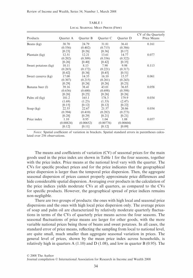
The means and coefficients of variation (CV) of seasonal prices for the maingoods used in the price index are shown in Table 1 for the four seasons, togetherwith the price index. Price means at the national level vary with the quarter. TheCVs for specific product prices and for the price indicates that the geographicalprice dispersion is larger than the temporal price dispersion. Then, the aggregateseasonal dispersion of prices cannot properly approximate price differences andhide considerable spatial dispersion. Averaging over products in the calculation ofthe price indices yields moderate CVs at all quarters, as compared to the CVsfor specific products. However, the geographical spread of price indices remainsnon-negligible.

There are two groups of products: the ones with high local and seasonal pricedispersions and the ones with high local price dispersion only. The average pricesof soap and palm oil are characterized by relatively moderate quarterly fluctua-tions in terms of the CVs of quarterly price means across the four seasons. Theseasonal fluctuations of price means are larger for other goods, with the morevariable national prices being those of beans and sweet potatoes. In all cases, thestandard error of price means, reflecting the sampling from local to national level,are quite small, much smaller than aggregate seasonal variation in prices. Thegeneral level of prices, shown by the mean price index across households, isrelatively high in quarters A (1.10) and D (1.08), and low in quarter B (0.95). The

TABLE 1

Local Seasonal Mean Prices (Frw)

Products Quarter A Quarter B Quarter C Quarter DCV of the Quarterly

Price Means

Beans (kg) 38.70 24.79 31.81 36.41 0.161(0.556) (0.402) (0.715) (0.386)[0.23] [0.26] [0.36] [0.17]

Plantain (kg) 12.51 12.21 13.61 14.77 0.077(0.202) (0.309) (0.356) (0.322)[0.26] [0.40] [0.42] [0.35]

Sweet potatoes (kg) 10.11 8.13 7.90 9.98 0.113(0.265) (0.172) (0.221) (0.317)[0.42] [0.34] [0.45] [0.51]

Sweet cassava (kg) 17.00 14.35 16.10 15.57 0.061(0.307) (0.215) (0.261) (0.243)[0.29] [0.24] [0.26] [0.25]

Banana beer (l) 39.16 38.41 43.01 36.85 0.058(0.636) (0.600) (0.698) (0.598)[0.26] [0.25] [0.26] [0.26]

Palm oil (kg) 181.2 165.1 178.3 179.9 0.034(1.69) (1.23) (1.33) (2.47)[0.15] [0.12] [0.12] [0.22]

Soap (kg) 22.55 22.67 21.57 20.86 0.034(0.394) (0.410) (0.282) (0.273)[0.28] [0.29] [0.21] [0.21]

Price index 1.10 0.95 1.04 1.08 0.057(0.00824) (0.00652) (0.00776) (0.00604)

[0.12] [0.11] [0.12] [0.09]

Notes: Spatial coefficient of variation in brackets. Spatial standard errors in parentheses calcu-lated over 256 observations.



34

months before the December–January harvests are those where the highest meanprices are reported (except for banana, banana beer and soap).

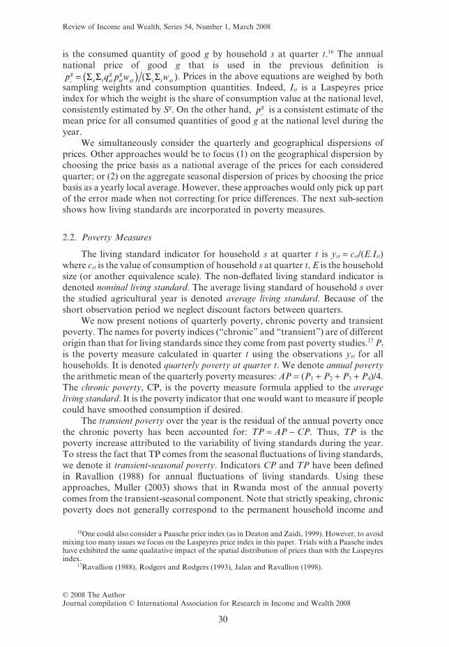
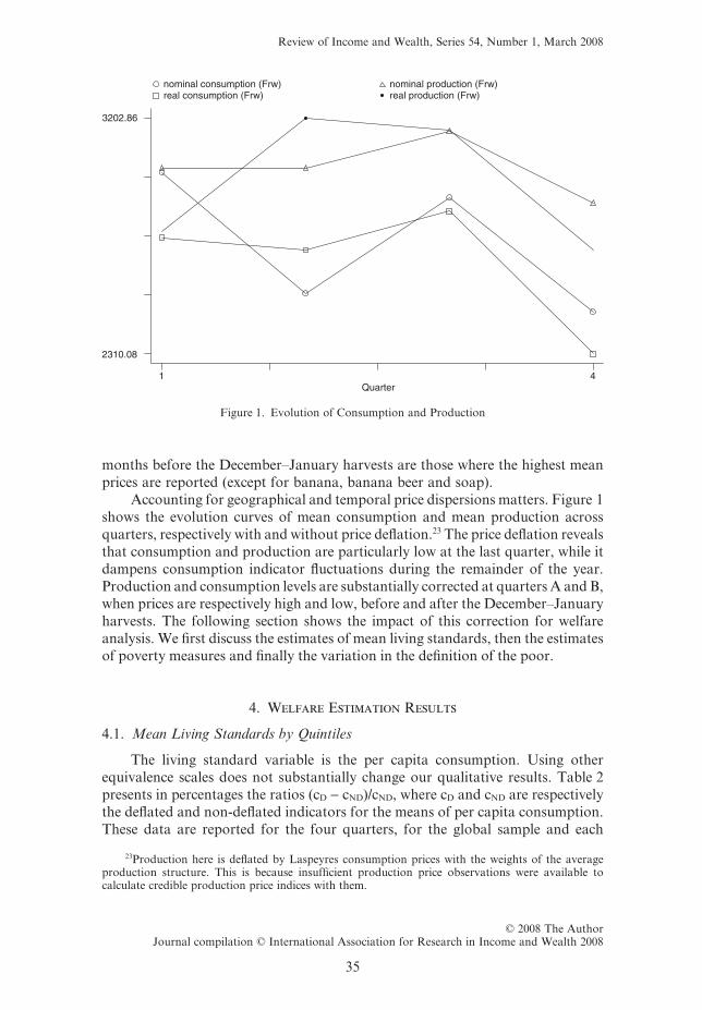
Accounting for geographical and temporal price dispersions matters. Figure 1shows the evolution curves of mean consumption and mean production acrossquarters, respectively with and without price deflation.23 The price deflation revealsthat consumption and production are particularly low at the last quarter, while itdampens consumption indicator fluctuations during the remainder of the year.Production and consumption levels are substantially corrected at quarters A and B,when prices are respectively high and low, before and after the December–Januaryharvests. The following section shows the impact of this correction for welfareanalysis. We first discuss the estimates of mean living standards, then the estimatesof poverty measures and finally the variation in the definition of the poor.

4. Welfare Estimation Results

4.1. Mean Living Standards by Quintiles

The living standard variable is the per capita consumption. Using otherequivalence scales does not substantially change our qualitative results. Table 2presents in percentages the ratios (cD - cND)/cND, where cD and cND are respectivelythe deflated and non-deflated indicators for the means of per capita consumption.These data are reported for the four quarters, for the global sample and each

23Production here is deflated by Laspeyres consumption prices with the weights of the averageproduction structure. This is because insufficient production price observations were available tocalculate credible production price indices with them.

Quarter

nominal consumption (Frw) nominal production (Frw) real consumption (Frw) real production (Frw)

1 4

2310.08

3202.86

Figure 1. Evolution of Consumption and Production



35

quintile of the annual per capita consumption.24 The results of t-tests of compari-sons of means25 show that at the national level, deflated mean living standards inquarters A, B and D are statistically different from non-deflated mean livingstandards in the same quarters. This is not the case for period C in which thedeflation with the price index is not significant (p-value = 0.14).

These features at least partially persist at the quintile level. Within eachquintile of the annual real living standard distribution, the effect of deflation ispervasive. The t-tests generally reject the hypothesis of equality of means. Then,the deflation is generally significant for estimating annual and quarterly meanliving standards in most quintiles. This is interesting since, most of the time, livingstandards statistics are published non-deflated in the reports of household surveys.Caution seems advisable when interpreting non-deflated results as genuine welfarestatistics.

However, the differences in these aggregates, with and without deflation, aremoderate, generally below 10 percent (on average over all quintiles: 9.1% inquarter A, -5.2% in B, 3.4% in C, 7.5% in D). Quarter D is unambiguously ahardship period: mean per capita consumption is lower whether measured with orwithout price deflation. For the first three quarters, these averages evolve moreregularly when deflated indicators are used, while the consumption fall is larger atthe last quarter with price adjustment. The latter results do not always persist atthe quintile level, which indicates that aggregate means might be misleading wherefluctuations in living standards are concerned.

Which dimension is the most relevant: geographical or seasonal variability? Avariance analysis shows that for both prices and living standards, the geographicalvariability contributes more to the explanation than the seasonal variability.However, both directions of variability must be considered when one wants tocompare with results caused by imperfect deflation for the whole year and thewhole country.

Finally, studying a single quarter could be sufficient for some purposes, suchas long term tracking of changes over years. However, the estimates in the nextsection will show that poverty in Rwanda is high at every quarter and all of themmust be observed for an accurate picture of poverty.

24Means and standard deviations of the per capita consumption are in Muller (2002).25See Wang (1971) for the calculus of the p-values of the tests with small samples.

TABLE 2

Percentages of Variation of Mean Per Capita Consumption((deflated – non-deflated)/non-deflated)

Variable Quarter A Quarter B Quarter C Quarter D

Per capita consumption (all quantiles) 8.91 -6.03 1.82 6.83Per capita consumption (Q = 1) 12.04 -4.65 6.02 9.72Per capita consumption (Q = 2) 6.56 -1.91 5.01 8.58Per capita consumption (Q = 3) 9.92 -5.47 5.29 8.16Per capita consumption (Q = 4) 7.82 -5.48 4.93 5.24Per capita consumption (Q = 5) 9.24 -8.69 -4.07 5.68

Notes: Q denotes the quintile of per capita consumption, respectively deflated and non-deflated.



36

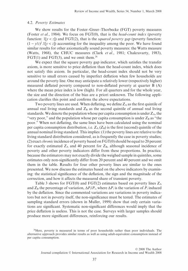
4.2. Poverty Estimates

We show results for the Foster–Greer–Thorbecke (FGT) poverty measures(Foster et al., 1984). We focus on FGT(0), that is the head-count index (povertyfunction: 1[y < z]) and FGT(2), that is the squared poverty gap (poverty function:(1 - y/z)2.1[y < z]) accounting for the inequality among the poor. We have foundsimilar results for other axiomatically sound poverty measures: the Watts measure(Watts, 1968), the CHUC measures (Clark et al., 1981; Chakravarty, 1983),FGT(1) and FGT(3), and we omit them.26

We expect that the square poverty gap indicator, which satisfies the transferaxiom, is more sensitive to price deflation than the head-count index, which doesnot satisfy this axiom. In particular, the head-count index should not be verysensitive to small errors caused by imperfect deflation when few households arearound the poverty line. One may anticipate a relatively lower (respectively higher)measured deflated poverty compared to non-deflated poverty at quarter B (A)where the mean price index is low (high). For all quarters and for the whole year,the size and the direction of the bias are a priori unknown. The following appli-cation clarifies this point and confirms the above expectations.

Two poverty lines are used. When deflating, we define ZA as the first quintile ofannual real living standards and ZB as the second quintile of annual real livingstandards. We denote the population whose per capita consumption is under ZA, the“very poor,” and the population whose per capita consumption is under ZB as “thepoor.” When not deflating, the same lines have been calculated using the nominalper capita consumption distribution, i.e. ZA (ZB) is the first (second) quintile of theannual nominal living standard. This implies: (1) the poverty lines are relative to theliving standard distribution considered, as is frequently the case in poverty studies;(2) exact chronic incidence of poverty based on FGT(0) should be equal to 20 percentfor exactly estimated ZA and 40 percent for ZB, although seasonal incidence ofpoverty and other poverty indicators differ from these proportions. In practice,because the estimators may not exactly divide the weighed sample in quintiles, someestimates only non-significantly differ from 20 percent and 40 percent and we omitthem in the table. Results for four other poverty lines are similar to the onespresented. We now discuss the estimates based on the above indicators by examin-ing: the statistical significance of the deflation, the sign and the magnitude of thecorrection, and how it affects the measured share of transient poverty.

Table 3 shows for FGT(0) and FGT(2) estimates based on poverty lines ZA

and ZB the percentage of variation, DPt/Pt, where DPt is the variation of Pt inducedby the deflation. Since the commented variations are variations in poverty indica-tors but not in poverty itself, the non-significance must be tested. The estimates ofsampling standard errors (shown in Muller, 1999) show that only certain varia-tions are significant. Systematic non-significant differences would imply that theprice deflation is useless. This is not the case. Surveys with larger samples shouldproduce more significant differences, reinforcing our results.

26Here, poverty is measured in terms of poor households rather than poor individuals. Thealternative approach provides similar results as well as using adult-equivalent consumption instead ofper capita consumption.



37

With these poverty lines, the price deflation brings significant changes inpoverty measures: a 10 percent change is not uncommon. For CP based on FGT(2),systematically significant results for changes are found with the upper (poverty) line,but not with the lower line. Changes in AP are significant at the 5 percent level forboth poverty measures with the upper line, but only for FGT(2) when using thelower line. Moreover, the deflation significantly affects quarterly poverty indicatorsat all quarters. Its impact is major at quarters A and B, in which the aggregate levelof prices is well apart the yearly average. The variations in TP are statisticallysignificant except for poverty incidence with the lower line. On the whole, even witha small sample, the local deflation is frequently significant for the two poverty lines,all poverty indicators and most quarters. This result is robust to using other povertylines and other poverty indicators. Let us turn to the sign of the correction.

The sign of DPt is positive, except in quarter B where the aggregate price indexis high and DPt is negative. However, we have checked with a larger set of povertylines that this sign cannot be systematically inferred, except in periods of largeaggregate price movements (quarters A and B). In part, this is due to the change inthe line accompanying the price deflation. The estimates are nonetheless oftenconsistent with a dominance of the effects of the aggregate price shifts acrossquarters.

The absolute magnitude of changes in poverty measures is considerable,notably for seasonal poverty in quarters A and B. However, this is not systematic

TABLE 3

Proportion of Changes in FGT(0) and FGT(2) PovertyMeasures Due to Local and Seasonal Price Deflation

Poverty Lines ZA ZA ZB ZB

FGT(0) FGT(2) FGT(0) FGT(2)P(A) 0.196** 0.377* 0.193* 0.393*P(B) -0.182* -0.199* -0.141* -0.149*P(C) 0.164* 0.102* 0.0850* 0.132*P(D) 0.0776* 0.131** 0.153* 0.177*AP 0.0531 0.0964* 0.0660* 0.129*CP 0.0363 0.0150 -0.0154 0.112*TP/AP 0.0390 0.0416* 0.783* 0.0149*

Notes: The numbers shown are: (poverty estimates deflated bylocal price indices)/(non-deflated poverty estimates) - 1, i.e. the pro-portionate effects of the deflation. Sampling standard errors for thedifferences are available in Muller (1999).

*Difference significant at 5% level; **difference significant at10% level.

FGT(0) is the head-count index and FGT(2) is the squaredpoverty gap. P(A), P(B), P(C), P(D) denote the poverty measures forthe successive quarters A, B, C, D of the agricultural year. AP is theannual poverty = (P(A) + P(B) + P(C) + P(D))/4. CP is the chronicpoverty. TP is the transient poverty. ZA is the poverty line equal to thefirst quintile of the annual per capita consumption (with or withoutdeflation). ZB is the poverty line equal to the second quintile of theannual per capita consumption (with or without deflation). As men-tioned in the text, changes in FGT(0) should be zero if the distribu-tions and the poverty lines were perfectly known instead of estimated.Here, they are insignificant even at the 10% level.



38

and depends on the poverty line and poverty indicator. The magnitude of changesin CP varies considerably (from -1.5 to 11.2 percent). The magnitude of changesin PA (19 to 39 percent) and in PB (-19 to -14 percent) is also substantial. Themagnitude of changes in PC (8 to 16 percent) and PD (7 to 18 percent) is smaller butstill non-negligible. When considering other lines, it appears that the impact of thedeflation depends much on the line, although it is generally sizeable. As expected,the relative changes caused by the deflation are larger in absolute value with thesquared poverty gap than with the head-count index. This is observed for AP, CPand quarterly poverty indicators.

Transient poverty is underestimated when not deflating. The change in themeasured share of transient poverty can sometimes be considerable (78 percent forthe head-count index and the lower line), although it is generally small (about 5percent). Non-deflated price dispersion hides part of the influence of the season-ality of living standards on annual poverty. This is consistent with the fact that atseasons with low agricultural output, living standards are low and food prices arehigh, and the opposite when output is high. We now look at the consequences ofthe deflation for anti-poverty targeting.

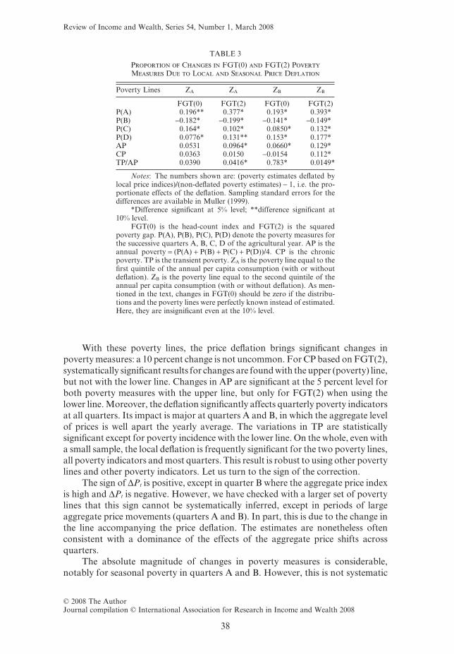
4.3. Variations in the Definition of the Poor

The deflation may change the measured composition of the population of thepoor even when the aggregate poverty measure is not significantly modified. InTable 4, the percentages of households that are considered poor before the defla-tion but not after, are shown in columns “Type I error” (for “false poor”).Columns “Type II error” (for “omitted poor”) show the percentages of households

TABLE 4

Variation in the Population of the Poor Caused by theDeflation (%)

Poverty Lines ZA ZA ZB ZB

Error type I II I IIAnnual FGT(0) (AP) 1.5 2.2 2.9 2.3Quarter A 0.67 5.13 0.36 7.46Quarter B 5.59 0.30 8.60 1.78Quarter C 2.57 6.52 2.36 5.64Quarter D 1.57 4.44 0.00 8.04

Notes: The first column (Type I error) for each poverty lineshows the percentage of households that are poor before the deflationand not after.

The second column (Type II error) for each poverty line showsthe percentage of households that are poor after the deflation and notbefore.

ZA is the poverty line equal to the first quintile of the annual percapita consumption (with or without deflation). ZB is the poverty lineequal to the second quintile of the annual per capita consumption(with or without deflation).

As mentioned in the text, changes in chronic FGT(0) should beexactly zero if the distributions and the poverty lines were perfectlyknown instead of estimated. Here, they are insignificant even at the10% level and not shown.



39

that are considered poor after the deflation but not before. For policy targeting,Type II is sometimes considered more important since some needy householdscannot be reached at all.

The size of changes in the definition of the poor that is caused by the deflationvaries. On the whole, Type I errors dominate. However, at the quarterly levelsubstantial changes in the definition of the poor can arise from both incorporatingand eliminating households. The pattern of changes in the poor population isaffected by the aggregate shift of the price index, although it is not sufficient toexplain it. In quarter A when the aggregate price index is high before the Januaryharvest, the Type II errors are more numerous than the Type I errors, while it is theopposite in quarter B. These results, which have been found for a larger set of lines,correspond to general underestimation or overestimation of poverty, dependingon the level of the aggregate price index. In contrast, when comparing the twoerror types for quarters C and D with an extended set of lines, no strong systematictendencies appear. Higher percentages of misclassified households are generallyobserved with higher lines, which is consistent with a larger proportion of the poorin the population.27 In the next section we compare results obtained by using localand regional prices.

5. Using Local or Regional Prices?

5.1. Statistical Tests and Estimates

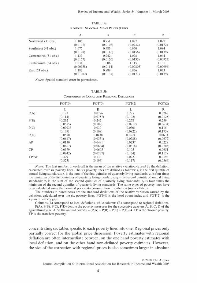
Regional price deflators, often used for welfare analysis, are not likely tointroduce distortions caused by quality choices as with local prices computed onhousehold budget data. Since Rwanda is divided in five agricultural regions (North-west, Southwest, Centrenorth, Centresouth, and East), the regional price indices aredefined as the mean price indices over each region. T-tests results show that theregional mean price index means significantly differ across regions and quarters,from 0.889 at quarter B in the East through 1.139 at quarter A in the Centrenorth.

They also show that regional price variation is generally significant for specificgoods. This occurs for all quarters and all representative products and the regionalprice means are sometimes far apart. Regional differences are less marked forbanana beer, palm oil and soap, widely traded throughout the country. Thestandard deviations of the product prices indicate that intra-regional price dis-persion at the same quarter is not negligible.

Table 5b shows the means and standard deviations of the relative variation inpoverty measures FGT(0) and FGT(2) induced respectively by local and regionaldeflations, calculated by considering six poverty lines altogether.28 It is a way of

27Unfortunately, the small sample size does not allow study of the characteristics of the poor thatwould have been overlooked when not deflating or when using inaccurate deflation.

28The six poverty lines are defined as follows: z1 is the first quintile of annual living standards; z2 isthe sum of the first quintiles of quarterly living standards; z3 is four times the minimum of the firstquintiles of quarterly living standards; z4 is the second quintile of annual living standards; z5 is the sumof the second quintiles of quarterly living standards; z6 is four times the minimum of the secondquintiles of quarterly living standards. The same types of poverty lines have been calculated using thenominal per capita consumption distribution (non-deflated). This implies that the lines are relative tothe living standards distribution considered.



40

concentrating six tables specific to each poverty lines into one. Regional prices onlypartially correct for the global price dispersion. Poverty estimates with regionaldeflation are often intermediate between, on the one hand poverty estimates withlocal deflation, and on the other hand non-deflated poverty estimates. However,the size of the correction with regional prices is also sometimes larger in absolute

TABLE 5a

Regional Seasonal Mean Prices (Frw)

A B C D

Northwest (37 obs.) 1.105 0.951 1.077 1.077(0.0107) (0.0106) (0.0232) (0.0172)

Southwest (41 obs.) 1.075 0.983 0.960 1.084(0.0198) (0.0116) (0.0156) (0.0139)

Centrenorth (51 obs.) 1.139 0.942 1.098 1.044(0.0157) (0.0120) (0.0135) (0.00927)

Centresouth (64 obs.) 1.034 1.006 1.115 1.131(0.00958) (0.0114) (0.00805) (0.00996)

East (63 obs.). 1.182 0.889 0.976 1.073(0.01902) (0.0137) (0.0177) (0.0139)

Notes: Spatial standard error in parentheses.

TABLE 5b

Comparison of Local and Regional Deflations

FGT(0) FGT(0) FGT(2) FGT(2)

L R L RP(A) 0.173 0.0776 0.275 0.0268

(0.114) (0.0757) (0.102) (0.0125)P(B) –0.232 –0.242 –0.258 –0.259

(0.0585) (0.109) (0.0712) (0.0634)P(C) –0.00933 –0.030 0.0301 –0.115

(0.107) (0.108) (0.0822) (0.175)P(D) 0.0570

(0.0617)0.0438(0.0331)

0.0624(0.0788)

0.0603(0.0672)

AP –0.0130 –0.0491 0.0237 –0.0228(0.0667) (0.0684) (0.0818) (0.0705)

CP –0.0579 –0.0605 –0.105 –0.0651(0.0842) (0.0737) (0.134) (0.117)

TP/AP 0.329 0.136 0.0227 0.0193(0.323) (0.196) (0.117) (0.0364)

Notes: The first number in each cell is the mean of the relative variation caused by the deflation,calculated over six poverty lines. The six poverty lines are defined as follows: z1 is the first quintile ofannual living standards; z2 is the sum of the first quintiles of quarterly living standards; z3 is four timesthe minimum of the first quintiles of quarterly living standards; z4 is the second quintile of annual livingstandards; z5 is the sum of the second quintiles of quarterly living standards; z6 is four times theminimum of the second quintiles of quarterly living standards. The same types of poverty lines havebeen calculated using the nominal per capita consumption distribution (non-deflated).

The numbers in parentheses are the standard deviations of the relative variation caused by thedeflation, calculated over the six poverty lines. FGT(0) is the head-count index and FGT(2) is thesquared poverty gap.

Columns (L) correspond to local deflations, while columns (R) correspond to regional deflations.P(A), P(B), P(C), P(D) denote the poverty measures for the successive quarters A, B, C, D of the

agricultural year. AP is the annual poverty = (P(A) + P(B) + P(C) + P(D))/4. CP is the chronic poverty.TP is the transient poverty.



41

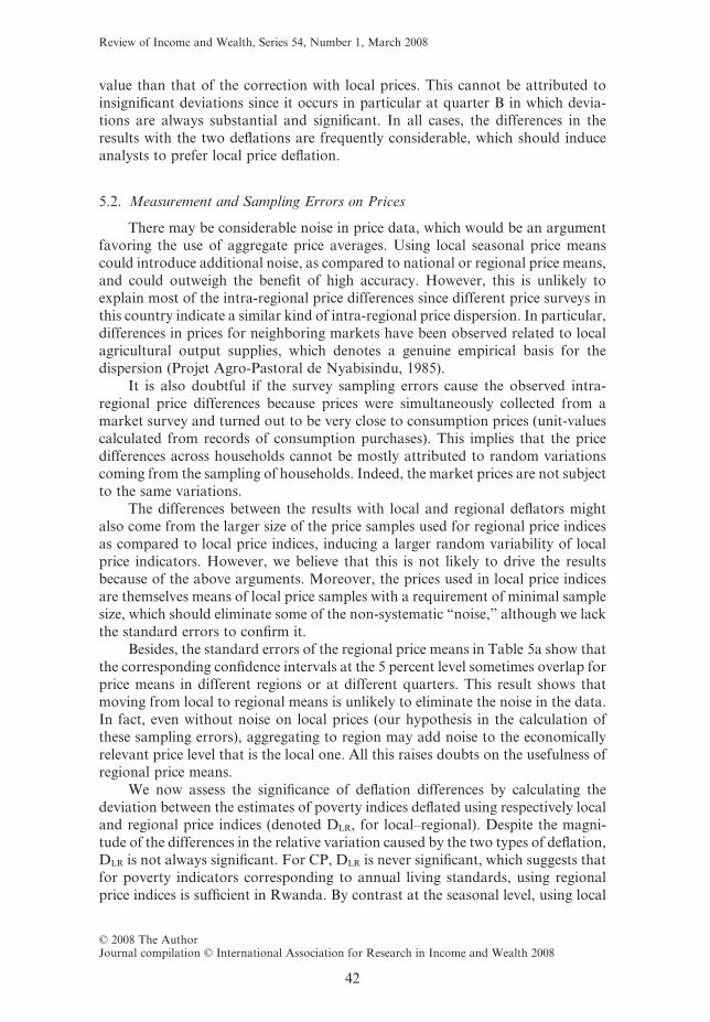
value than that of the correction with local prices. This cannot be attributed toinsignificant deviations since it occurs in particular at quarter B in which devia-tions are always substantial and significant. In all cases, the differences in theresults with the two deflations are frequently considerable, which should induceanalysts to prefer local price deflation.

5.2. Measurement and Sampling Errors on Prices

There may be considerable noise in price data, which would be an argumentfavoring the use of aggregate price averages. Using local seasonal price meanscould introduce additional noise, as compared to national or regional price means,and could outweigh the benefit of high accuracy. However, this is unlikely toexplain most of the intra-regional price differences since different price surveys inthis country indicate a similar kind of intra-regional price dispersion. In particular,differences in prices for neighboring markets have been observed related to localagricultural output supplies, which denotes a genuine empirical basis for thedispersion (Projet Agro-Pastoral de Nyabisindu, 1985).

It is also doubtful if the survey sampling errors cause the observed intra-regional price differences because prices were simultaneously collected from amarket survey and turned out to be very close to consumption prices (unit-valuescalculated from records of consumption purchases). This implies that the pricedifferences across households cannot be mostly attributed to random variationscoming from the sampling of households. Indeed, the market prices are not subjectto the same variations.

The differences between the results with local and regional deflators mightalso come from the larger size of the price samples used for regional price indicesas compared to local price indices, inducing a larger random variability of localprice indicators. However, we believe that this is not likely to drive the resultsbecause of the above arguments. Moreover, the prices used in local price indicesare themselves means of local price samples with a requirement of minimal samplesize, which should eliminate some of the non-systematic “noise,” although we lackthe standard errors to confirm it.

Besides, the standard errors of the regional price means in Table 5a show thatthe corresponding confidence intervals at the 5 percent level sometimes overlap forprice means in different regions or at different quarters. This result shows thatmoving from local to regional means is unlikely to eliminate the noise in the data.In fact, even without noise on local prices (our hypothesis in the calculation ofthese sampling errors), aggregating to region may add noise to the economicallyrelevant price level that is the local one. All this raises doubts on the usefulness ofregional price means.

We now assess the significance of deflation differences by calculating thedeviation between the estimates of poverty indices deflated using respectively localand regional price indices (denoted DLR, for local–regional). Despite the magni-tude of the differences in the relative variation caused by the two types of deflation,DLR is not always significant. For CP, DLR is never significant, which suggests thatfor poverty indicators corresponding to annual living standards, using regionalprice indices is sufficient in Rwanda. By contrast at the seasonal level, using local



42

deflation instead of regional deflation is crucial for estimating quarterly poverty inquarters A and C, but not in quarters B and D. Almost all cases where DLR issignificant correspond to underestimation of poverty when using regional prices.This is consistent with a local concentration of the poor in areas far from marketsand transaction sites. On the whole, the current practice of developing pricedeflators only for a few regions is not reliable when studying seasonal poverty, atleast in Rwanda, although the bias may be neglected for chronic annual poverty.

Similarly, we investigated the magnitude of the mistake made relative to thedifference between quarterly and annual prices (see Muller, 1999, for tables andcomment). Here again, we find that using price indicators at the lowest level ofaggregation is essential. In particular, the share of transient poverty is biasedupward by using annual prices.

6. Concluding Remarks

Static and dynamic welfare indicators are generally imperfectly corrected forprice dispersion across households and seasons. To our knowledge, the importanceof price correction at local and seasonal level for welfare measurement has notbeen empirically studied in the literature.

Using seasonal panel data from rural Rwanda, we show the importance of anaccurate price deflation based on local and seasonal prices. In many instances, theprice deflation significantly changes the measured mean living standards andpoverty indicators, whether quarterly, chronic or transient. However, if changes inmeasured aggregate living standards are moderate in every quarter, this is notalways the case for measured poverty, for which the magnitude of changes can beconsiderable. The structure of welfare changes is also affected by the deflation.Mean living standards and poverty measures appear to vary more smoothly alongthe year when based on accurately deflated living standards, but then they alsoshow better the severe welfare crisis after the dry season in Rwanda.

In terms of the impact of price deflation on poverty assessment, the choice ofthe poverty line and the considered quarter are generally more influential than thechoice of the poverty indicator. At some quarters the effects of aggregate seasonalfluctuations of prices can dominate the effect of geographical price dispersion toimply substantial and unambiguously positive or negative variations of povertymeasures in these periods when deflation is implemented. Poverty indicators stress-ing on poverty severity are more likely to deliver powerful deflation effects. More-over, the deflation modifies the composition of the population of the poor andtherefore affects anti-poverty targeting.

The comparison with poverty indicators deflated using regional price indicesinstead of local price indices shows that when studying seasonal poverty, regionalprice indices provide an imperfect correction only. If the bias caused by usingregional prices is minor for the measurement of chronic and annual poverty inRwanda, it is not the case when estimating quarterly poverty. Similarly, usingannual prices instead of quarterly prices produces not only severely biased mea-sures of seasonal and transient poverty, but also underestimates annual andchronic poverty. Using regional and annual prices is just not good enough foraccurate poverty analysis in Rwanda.



43

When is accurate deflation needed from a policy perspective? Our resultssuggest that in contrast with the common practice of using regional or annualprice correction, detailed price statistics are important in monitoring of policiesagainst poverty. They are particularly useful for guiding first, policies againstseasonal and transient poverty since seasonal and transient poverty measures aremore sensitive to deflation; and second, policies directed against poverty severityas opposed to policies only aiming at reducing the number of the poor. Mean-while, the impact of the deflation on measured mean living standards and thesensitivity of results to the choice of the poverty line show that growth policiesand aggregate demand policies addressing problems at different levels of the livingstandard distribution would be better served by living standard statistics that areaccurately deflated.

To fully understand why the results are the way they are, and how thecharacteristics of Rwanda influence the misleading picture of poverty obtainedwhen not properly deflating, we would need a complete explanation of seasonaland geographical distribution of prices in Rwanda and of its links with the livingstandard distribution across seasons. Also, our results are based on a particularcountry at a specific period. Clearly, they show that in that case accurate geo-graphical and temporal deflation is necessary to robust welfare analysis. However,more studies would be necessary to: (1) elucidate the precise economic mechanismsinvolved; and (2) generalize the findings to other countries and periods. Also, moresophisticated price indices anchored on utility levels could be considered, althoughit is not at the moment common practice in LDCs.

Appendix 1: Sampling Standard-Error Estimators

The complexity of the actual sampling scheme does not allow us a robust useof classical sampling variance formula. We use an estimator for sampling standarderrors that is a combination of “linearization” estimators obtained using balancedrepeated replications (Krewski and Rao, 1981; Roy, 1984; Shao and Rao, 1993)and that is simpler and quicker than stratified bootstrap procedures. Howes andLanjouw (1998) have shown that the sampling design can modify the estimatedstandard errors for poverty measures. Consequently, our estimators for the sam-pling standard errors account for the sample design. Note also that becausedeflated and non-deflated welfare measures are based on the same sample ofobservations, their difference, which is the difference of a mean over the samesample, is equal to the mean of the difference over this sample. Then, tests of thedifference are simply tests of this significance of this difference and involve similarcalculations to the sampling standard errors for the poverty measures.

The poverty indicator of a sub-population is estimated by a ratio of the type

′ = ′′

yzxx

where ′denotes the Horwitz–Thompson estimator for a total (sum of values for thevariable of interest weighted by the inverse of the inclusion probability). z is thesum of the poverty in the sub-population and x is the size of the sub-population.The variance associated with the sampling error is then approximated by:



44

V y = V z 2 y Cov z x + y V x x x x x′( ) ′( ) − ′ ′ ′( ) ′( ) ′( )⎡⎣

⎤⎦ ′( ),

2 2

obtained from a Taylor expansion at the first order from function Y = f(Z/X)around (Ey�, Ex�) and because Ez� � 0 and x� does not cancel, where the appro-priate expectations are estimated by x� and ′yx

.We divide the sample of communes (first actual stage of the sampling since all

the prefectures are drawn) in five super-strata (a = 1 to 5) so as to group togetherthe communes sharing similar characteristics, and to a priori reduce the varianceintra-strata. Several sectors are assumed to have been drawn in each strata. Thisallows the estimation of the variance intra-strata, while the calculation of thevariance intra-commune was impossible, since in fact only one sector had beendrawn in each commune. Then, the Horwitz–Thompson formula for super-strataa is:

′ ∑ ∑ ∑∑= ==

z = Mm

Nn

Q

qz

h

hh

hi

hii

mhij

hij

hijkk

q

j

nh hijhi

αα

α

1 11

aand

′ ∑ ∑ ∑∑= ==

x = Mm

Nn

Q

qx

h

hh

hi

hii

mhij

hij

hijkk

q

j

nh hijhi

αα

α

1 11

where Mh is the number of communes in prefecture h; mha is the number of com-munes in prefecture h and drawn in super-strata a; Nhi is the number of sectors incommune i of prefecture h and super-strata a; nhi is the number of sectors drawnin commune i of prefecture h and super-strata a; Qhij is the number of householdsin sector j of commune i of prefecture h; qhij is the number of households drawn insector j of commune i of prefecture h and super-strata a. Similar formulae can beused to account for the intermediary drawing of one district in every sector.

Cov(z�, x�) is estimated by:

ˆ ,Cov z x = z z x x ′ ′( ) ′ − ′( )⋅ ′ − ′( )=1

∑120 α α

α

5

and similar formulae for V(x) and V(z) are obtained by making x = z.

Appendix 2: Properties of the Elementary Price Samples

A preliminary analysis of the consumption price means and the market pricemeans has shown that these indicators are very close and cannot be systematicallyordered. These two latter types of price indicators have different qualities. Marketprice surveys are believed to provide price information that is less dependent fromhousehold tastes and purchasing power by better controlling quality choices.However, since price observations are collected only in selected sites, they mayprovide inaccurate estimates of the prices to which some households are con-fronted. Moreover, the wording of the questions and the whole collection processof prices are always debatable in that they constitute an artificial observationsituation, different from what occurs during actual transactions. Finally, it is neverpossible to obtain price observations for all goods in all selected markets ortransaction sites. This means that the treatment of missing values for prices is an



45

important stage of using market price data. Furthermore, even when price obser-vations are available, the analyst is not content to use them if they are isolated. Alarge sample of price observations is in fact necessary and what is called “marketprice” in the price data file is a central tendency of this sample, the mean or themedian of observed prices.

When budget data are used to calculate prices, the information about pricesfits more closely the consumption pattern of the household. Indeed, goods that areusually consumed in an area generally appear in purchase or sale transactions,even when they are only consumed in kind (from their own production or receivedas gift) by some of the households of this area. Unfortunately, the prices extractedfrom a budget survey are in fact elementary “unit-values,” i.e. ratios of values overquantity extracted from observations of individual transactions. Elementary unit-values are believed to be affected by quality choices of consumers or sellers. In thatsituation, a higher level of prices for a specific household might come from a higherquality of its consumption. Moreover, consumption data is known to incorporatelarge measurement errors that can be amplified by the use of unit-values instead ofexogenous prices. Of course, when no price data are available, unit-values Laspey-res indices might well be better than no correction at all.

This problem for elementary goods is much less serious than for unit-valuescalculated from categories of consumption, as in Deaton (1988, 1990), wheresimilar goods are aggregated in a common category, for example “fish.” In thelatter case the unit-value calculated from these aggregate values and quantities haslittle in common with the observed prices in a market (the price of a specific fish).However, even if one expects it to be here relatively minor with specific goods, thequality choice remains.

Appendix 3: Selection of the Price Indicators

Price Database

Three types of prices are in the database. First, the consumption prices aremean prices for each commodity, calculated from the records of consumptionpurchases. The means are weighed by using the sampling scheme and the con-sumption levels of surveyed households for the considered good as shown above,while at the cluster level instead of the national level. Second, the production pricesare mean prices for each product, calculated from the records of household pro-duction sales. Here, the means are weighed by using the sampling scheme and theproduction level of the surveyed households for the considered product. Third,market prices are unweighed means from the price survey in the markets ortransaction sites near the location of the surveyed households.

Market prices were collected once every quarter at the middle of the dailyinterviews of households in a cluster. The collection took place in the closestmarkets where the surveyed households had declared that they make most of theirpurchases. The information was obtained by interviews with sellers and weighingof the products. Therefore, the market prices are based on actual values ratherthan price announcements. Once a sufficient number of prices has been collectedamong several important sellers in the market, the market price of this product is



46

calculated as the arithmetic mean of these observations after outlier values havebeen eliminated. Because each household is surveyed daily during two weeks, theseprices can be considered as fortnight prices.

Because of the small differences in production prices and consumption prices,market price means and consumption price means at the cluster level are accept-able approximations of shadow prices and are used where possible in the calculusof price indices.

Despite their relative proximity, there are several reasons to use consumptionprices and market prices rather than production prices. First, the date of theinformation present in the questionnaire corresponds better to the actual consump-tion when using consumption prices or market prices. Indeed, in each sector theseprices are collected during the same week as most of the consumption information,while the production prices are calculated from sale transactions often based onquarterly retrospective records. Second, the final consumption of the goods corre-sponding to the actual observation of consumption prices and market prices isalmost contemporary to the price observations, whereas the observed sales onwhich are based the production prices may sometimes be the object of consump-tion, only much later, after several trade intermediations, and sometimes out of theconsidered district. Third, we want to avoid mixing the two types of price means(consumption price and market price means vs. production price means, because ofthe slightly lower level of production prices). The sample of observations ofproduction prices is much smaller. It is therefore logical to eliminate it to base theanalysis on the sample of consumption prices and market prices.

Replacement of Missing Values

Firewood has been eliminated from the consumption (2.9 percent of theaggregate consumption), because the corresponding price means are missing in toomany clusters. For the other categories the mean price of a representative productis sometimes missing because of infrequent consumption of the product in theconsidered cluster. This is attributed to penury of the product, the consumptiondemand fluctuating less than the production supply for seasonal agricultural prod-ucts. In that case, the price of the product should be higher than usual and we usedthe larger sector price mean observed in the same region as an approximation.

References

André, C. and J.-P. Platteau, “Land Relations Under Unbearable Stress: Rwanda Caught in theMalthusian Trap,” Journal of Economic Behaviour & Organization, 34(1), 1–47, 1998.

Appleton, S., “Changes in Poverty in Uganda, 1992–1997,” in P. Collier and R. Reinnikka (eds), Firms,Households and Government in Uganda’s Recovery, World Bank, Washington DC, 2001.

Atkinson, A. B., “On the Measurement of Poverty,” Econometrica, 55(4), 749–64, 1987.Bane, M. J. and D. Ellwood, “Slipping Into and Out of Poverty: The Dynamics of Spells,” Journal of

Human Resources, 21(1), 1–23, 1986.Baris, P. and P. Couty, “Prix, marchés et circuit commerciaux africains,” AMIRA No. 35, December

1981.Baulch, R. and J. Hoddinot, “Economic Mobility and Poverty Dynamics in Developing Countries,”

Journal of Development Studies, 36(6), 1–24, 2000.Betson, D. M., C. F. Citro, and R. T. Michael, “Recent Developments for Poverty Measurement in

U.S. Official Statistics,” Journal of Official Statistics, 16(2), 87–111, 2000.



47

Blaine, R. and M. Sosulski, “Adjusting Thresholds for Geographic Areas,” mimeo, Wisconsin Uni-versity, 2002.

Bulletin Climatique Du Rwanda, Climatologie et Précipitations, Kigali, Rwanda, 1982, 1983, 1984.Bureau National du Recensement, Recensement de la Population du Rwanda, 1978. Tome 1: Analyse,

Kigali, Rwanda, 1984.Bylenga, S. and S. Loveridge, “Intégration des prix alimentaires au Rwanda, 1970–86,” Note SESA,

Kigali, Rwanda, 1988.Chakravarty, S. R., “A New Index of Poverty,” Mathematical Social Science, 6, 307–13, 1983.Citro, C. F. and R. T. Michael, Measuring Poverty. A New Approach, National Academic Press,

Washington DC, 1995.Clark, S., R. Hemming, and D. Ulph, “On Indices for the Measurement of Poverty,” Economic Journal,

91, 515–26, 1981.Danziger, L., “Inflation, Fixed Cost of Price Adjustment, and Measurement of Relative-Price Vari-

ability: Theory and Evidence,” The American Economic Review, 77(4), 703–10, 1987.Deaton, A., “Quality, Quantity, and Spatial Variation of Price,” The American Economic Review, 78,

418–30, 1988.———, “Price Elasticities from Survey Data. Extensions and Indonesian Results,” Journal of Econo-

metrics, 44, 281–309, 1990.———, “Getting Prices Right: What Should Be Done?” Journal of Economic Perspective, 12(1), 37–46,

1998.———, “Prices and Poverty in India 1987–2000,” Economic and Political Weekly, 362–8, January 25,

2003.Deaton, A. and A. Tarozzi, “Prices and Poverty in India,” mimeo, Princeton University, July 2000.Deaton, A. and S. Zaidi, “Guidelines for Constructing Consumption Aggregates for Welfare Analy-

sis,” mimeo, The World Bank, 1999.Dercon, S. and P. Krishnan, “Changes in Poverty in Rural Ethiopia 1989–1995: Measurement, Robust-

ness Tests and Decomposition,” Discussion Paper CSAE, March 1998.Domberger, S., “Relative Price Variability and Inflation: A Disaggregated Analysis,” Journal of

Political Economy, 95(31), 547–66, 1987.Expert Group on Household Income Statistics, The Camberra Group. Final Report and Recommenda-

tions, Australian Bureau of Statistics, 2000.Foster, J., J. Greer, and E. Thorbecke, “A Class of Decomposable Poverty Measures,” Econometrica,

52(3), 761–6, 1984.Gabriel, E., “Carte des marchés agricoles du Rwanda,” Note technique no. 5 de l’ISAR, Kigali,

Rwanda, 1973.———, “Evolution des prix des diverses marchandises sur des marchés Rwandais,” Note technique no.

14 de l’ISAR, Kigali, Rwanda, 1974.Gibson, J., “A Simple Test of Liquidity Constraints and Whether the Poor Pay More,” mimeo,

University of Waikato, 2006a.———, “Prices and Unit Values in Poverty Measurement and Tax Reform Analysis,” mimeo, Uni-

versity of Waikato, 2006b.Glewwe, P., “The Measurement of Income Inequality under Inflation,” Journal of Development Eco-

nomics, 32, 43–67, 1990.Glezakos, C. and J. B. Nugent, “A Confirmation of the Relation between Inflation and Relative Price,”

Journal of Political Economy, 94(41), 895–9, 1986.Grimm, M. and I. Günther, “Growth and Poverty in Burkina Faso. A Reassessment of the Paradox,”

Journal of African Economies, 16(1), 70–98, 2007.Grootaert, C. and R. Kanbur, “A New Regional Price Index for Cote d’Ivoire using Data from the

International Comparison Project,” Journal of African Economies, 3(1), 114–41, 1994.———, “Regional Price Differences and Poverty Measurement,” in C. Grootaert (ed.),

Analyzing Poverty and Policy Reform. The Experience of Cote d’Ivoire, Avebury, Brookfield, USA,1996.

Günther, I. and M. Grimm, “Measuring Pro-Poor Growth When Relative Prices Shift,” Journal ofDevelopment Economics, 82, 245–56, 2007.

Howes, S. and J. O. Lanjouw, “Does Sample Design Matter for Poverty Rate Comparisons,” Reviewof Income and Wealth, 44(1), 1998.

Jalan, R. and M. Ravallion, “Transient Poverty in Post-reform Rural China,” Journal of ComparativeEconomics, 26, 338–57, 1998.

Jazairy, I., M. Alamgir, and T. Panuccio, “The State of World Rural Poverty,” Intermediate Techn-ology Publications, New York University Press, New York, 1992.

Kakwani, N. and R. J. Hill, “Economic Theory of Spatial Cost of Living Indices with Application toThailand,” Journal of Public Economics, 86, 71–97, 2002.



48

Krewski, D. and J. N. K. Rao, “Inference from Stratified Sample,” Annals of Statistics, 9, 1010–9, 1981.Lipton, M. and M. Ravallion, “Poverty and Policy,” in J. Behrman and T. N. Srinivasan (eds),

Handbook of Development Economics, vol. 3, North Holland, Amsterdam, 1993.Ministère du Plan, Méthodologie de la Collecte et de l’échantillonnage de l’Enquête Nationale sur le

Budget et la Consommation 1982–83 en Milieu Rural, Kigali, 1986a.———, Enquête des Prix PCI au Rwanda, Kigali, 1986b.Muellbauer, J., “Inequality Measures, Prices and Household Composition,” Review of Economic

Studies, 41(4), 493–502, 1974.Muller, C., E.N.B.C.: Relevés de prix en milieu rural, Ministère du Plan, Kigali, Rwanda, 1988.———, “The Measurement of Poverty with Geographical and Intertemporal Price Dispersion,”

CREDIT Working Paper, May 1999.———, “Prices and Living Standards. Evidence for Rwanda,” Journal of Development Economics, 68,

187–203, 2002.———, “The Share of Seasonal Transient Poverty. Evidence from Rwanda,” Working Paper, WP-AD

2003-39, University of Alicante, 2003.———, “The Valuation of Non-Monetary Consumption in Household Surveys,” Social Indicators

Research, 72(3), 319–41, 2005.Niyonteze, F. and A. Nsengiyumva, Dépouillement et présentation des résultats de l’enquête sur marchés

Projet Kigali-Est, Projet Kigali-Est, June 1986.O.S.C.E., Note statistique rapide sur la comparaison des niveaux des prix du Rwanda, O.S.C.E., Brussels,

1987.Pritchett, L., Y. Suharso, S. Sumarto, and A. Suryahadi, “The Evolution of Poverty During the Crisis

in Indonesia, 1996 to 1999,” mimeo, Social Monitoring and Early Response Unit, World Bank,Washington DC, 2000.

Projet Agro-Pastoral de Nyabisindu, “Commercialisation des produits agricoles (marchés et prix),”Etudes et Expériences No. 6, Kigali, Rwanda, 1985.

Ravallion, M., “Expected Poverty under Risk-Induced Welfare Variability,” The Economic Journal, 98,1171–82, 1988.

———, Poverty Comparisons. A Guide to Concepts and Methods, Harwood Academic Publishers,London, 1994.

Ravallion, M. and B. Bidani, “How Robust is a Poverty Profile?” The World Bank Economic Review,8(1), 75–102, 1994.

Ravallion, M. and S. H. Chen, “When Economic Reform is Faster than Statistical Reform: Measuringand Explaining Income Inequality in Rural China,” Oxford Bulletin of Economics and Statistics,61(1), 33–48, 1999.

Riley, H. E., “Some Aspects of Seasonality in the Consumer Rice Index,” American Statistical Asso-ciation Journal, 56(293), 27–37, 1961.

Rodgers, J. R. and J. L. Rodgers, “Chronic Poverty in the United States,” Journal of Human Resources,XVIII(1), 1993.

Roy, G., “Enquête Nationale Budget Consommation Rwanda: Plan de sondage,” INSEE, Départe-ment de la Coopération, May 1984.

Shao, J. and J. N. K. Rao, “Standard Errors for Low Income Proportions Estimated from StratifiedMulti-Stage Samples,” Sankhya: The Indian Journal of Statistics, 55, Series B, Part 3, 393–414,1993.

Slesnick, D. T., “Gaining Ground: Poverty in the Post-war United States,” Journal of PoliticalEconomy, 101(1), 1993.

Stevens, A. H., “The Dynamics of Poverty Spells: Updating Bane and Ellwood,” A.E.A. Papers andProceedings, 84(2), May 1994.

Tang, D.-P. and P. Wang, “On Relative Price Variability and Hyperinflation,” Economic Letters, 42,209–14, 1993.

The World Bank, World Development Report 1990. Poverty, Oxford University Press, 1990.———, World Development Report 2000/2001. Attacking Poverty, Oxford University Press, 2000.Wang, Y. Y., “Probabilities of the Type I Errors of the Welch Tests for the Behrens–Fisher Problem,”

Journal of the American Statistical Association, 66(335), 605–8, 1971.Watts, H. W., “An Economic Definition of Poverty,” in D. P. Moynihan (ed.), On Understanding

Poverty, Basic Books, New York, 316–29, 1968.White, A. G., “Measurement Biases in Consumer Price Indexes,” International Statistical Review,

67(3), 301–25, 1999.Wilkerson, M., “Sampling Error in the Consumer Price Index,” Journal of the American Statistical

Association, 62(319), 899–914, 1967.



49

the measurement of poverty with geographical and intertemporal price dispersion: evidence from...

Documents