OPERATIONS RESEARCHArticles in Advance, pp. 1–25ISSN 0030-364X (print) ó ISSN 1526-5463 (online) https://doi.org/10.1287/opre.2016.1548

©2016 INFORMS

Intertemporal Pricing Under Minimax Regret

René Caldentey

Booth School of Business, University of Chicago, Chicago, Illinois 60637, rene.caldentey@chicagobooth.edu

Ying Liu, Ilan Lobel

Stern School of Business, New York University, New York, New York 10012 {yliu2@stern.nyu.edu, ilobel@stern.nyu.edu}

We consider the pricing problem faced by a monopolist who sells a product to a population of consumers over a finite timehorizon. Customers’ types differ along two dimensions: (i) their willingness-to-pay for the product and (ii) their arrivaltime during the selling season. We assume that the seller knows only the support of the customers’ valuations and donot make any other distributional assumptions about customers’ willingness-to-pay or arrival times. We consider a robustformulation of the seller’s pricing problem that is based on the minimization of her worst-case regret. We consider twodistinct cases of customers’ purchasing behavior: myopic and strategic customers. For both of these cases, we characterizeoptimal price paths. For myopic customers, the regret is determined by the price at a critical time. Depending on theproblem parameters, this critical time will be either the end of the selling season or it will be a time that equalizes theworst-case regret generated by undercharging customers and the worst-case regret generated by customers waiting for theprice to fall. The optimal pricing strategy is not unique except at the critical time. For strategic consumers, we developa robust mechanism design approach to compute an optimal policy. Depending on the problem parameters, the optimalpolicy might lead some consumers to wait until the end of the selling season and might price others out of the market.Under strategic customers, the optimal price equalizes the regrets generated by different customer types that arrive at thebeginning of the selling season. We show that a seller that does not know if the customers are myopic should price asif they are strategic. We also show there is no benefit under myopic consumers to having a selling season longer than acertain uniform bound, but that the same is not true with strategic consumers.

Keywords : demand uncertainty; strategic consumers; robust optimization; prior-free; worst-case regret.Subject classifications : marketing: pricing; games/group decisions: noncooperative; programming.Area of review : Operations and Supply Chains.History : Received November 2013; revisions received April 2015, April 2016; accepted June 2016. Published online in

Articles in Advance November 7, 2016.

1. Introduction

Over the last couple of decades, dynamic pricing has beentransformed from a curious and somewhat controversialpractice used primarily by upstart airlines into a techniquethat is widely used in a variety of industries. As technol-ogy has evolved and reduced menu costs, retailers of allsorts have adopted intertemporal pricing practices. One ofthe key economic drivers behind the rapid disseminationof dynamic pricing is demand uncertainty: there is enor-mous value for a firm in being able to change prices overtime in situations where the firm does not know how muchcustomers are willing to pay for its products.

In response to the increasing use of dynamic pricing inpractice, academics have proposed a variety of techniquesfor algorithmically determining intertemporal pricing poli-cies. However, the vast majority of these approaches requirethe firm to know the probability distributions of customervaluations and arrival times. Assuming that the firm knowsa full probabilistic model of customer valuations and arrivaltimes is problematic for at least two reasons. The first rea-son is the obvious one: firms do not have access to suchprobability distributions; even when they have sales data,

they typically do not have access to a data set that is richenough to estimate valuation and arrival time distributions.The second reason is less obvious but equally important:taking the probability distributions of customer valuationsand arrival times as given assumes away a significant partof the lack of knowledge about customer valuations andarrival times.These issues are especially acute for firms introducing

new products into the marketplace. When firms launch newproducts, they usually have very little information abouthow much customers are willing to pay for them. This greatdegree of uncertainty makes new products excellent can-didates for dynamic pricing strategies. However, the sameuncertainty about customer valuations also hobbles ourability to use established dynamic pricing techniques sincethey rely on the firm knowing the probability distribution ofcustomer valuations. Pricing of new products is no trivialmatter. For instance, a McKinsey study reported that morethan a 100,000 new products are introduced yearly into theU.S. retail industry, but 70%–80% of these launches fail.The use of dynamic pricing for new products can reducethe impact of demand uncertainty on the firm and, in thisway, help some of these launches succeed.

1

Dow

nloa

ded

from

info

rms.o

rg b

y [1

28.1

22.1

49.1

54] o

n 26

Janu

ary

2017

, at 1

8:23

. Fo

r per

sona

l use

onl

y, a

ll rig

hts r

eser

ved.

Caldentey, Liu, and Lobel: Intertemporal Pricing Under Minimax Regret2 Operations Research, Articles in Advance, pp. 1–25, © 2016 INFORMS

We approach the problem of intertemporal pricing fromthe perspective of robust optimization (see Bertsimas andSim 2004, Ben-Tal et al. 2009). Specifically, we assumethat the seller only knows the range of customers’ valua-tion (or willingness to pay) for its product and makes noadditional assumptions about their distribution or about thecustomers’ arrival process. The formulation we propose isquite parsimonious, but still sufficiently rich to give rise todifferent types of pricing policies for different sets of prob-lem parameters. Our model formulation can be used both insettings with limited information, where the firm has only avery rough guess of the customer’s range of valuations, aswell as in an environment that is more data-rich, where thefirm can use sales data to estimate an uncertainty set of thecustomers’ valuations. It is also flexible enough to allowus to study optimal pricing policies for myopic as well asstrategic customers, the latter being customers who timetheir purchases to maximize their own discounted utilities.

Under such a minimalist informational structure, thestandard expected profit maximization criterion is not ap-propriate as the seller’s objective function (for more details,see Section 2). Instead, we consider the seller’s regret,which is defined as the difference between her payoff underfull demand information and her realized payoff. In this set-ting, an optimal pricing strategy is one that minimizes thedifference between the seller’s ex-post payoff and that of aclairvoyant who sets prices knowing customer types (valu-ation and arrival time) in advance. In particular, we assumethe seller chooses a policy that minimizes her worst-caseanticipated ex post regret. The seller assumes that natureselects customer types from the uncertainty set to gener-ate as much regret as possible, and that customers behaveeither myopically or strategically with respect to prices.The first paper to propose a minimax regret criterion forpricing without a prior distribution over customer valua-tions was Bergemann and Schlag (2008). Our approachcan be seen as an intertemporal version of Bergemann andSchlag (2008)’s static model.

We make several modeling assumptions that we wish tohighlight before we discuss our contributions. First, we donot include inventory considerations in our model. Havingthe customers strategically consider availability risk wouldrequire us to model customers’ beliefs about each other’sstrategies, and thus make our model less parsimonious. Toreduce the number of parameters in our model and maintaintractability, we also assume the seller and the consumersdiscount the future at the same rate, and that all consumerscan be described by the same uncertainty set. We do allowfor a mix of strategic and myopic consumers to be presentin the market (see Section 6). Furthermore, we assume thefirm has full commitment power. Minimax regret withoutcommitment leads to a problem of dynamic inconsistency,which is not amenable to a Bellman-equation approach (seeHayashi 2009), and is thus likely an intractable problem.For a more detailed discussion on our commitment assump-tion, see Section 2.

1.1. Contributions

The primary contribution of this paper is the developmentof a robust optimization methodology to compute intertem-poral pricing policies that minimize a firm’s worst-caseregret when selling to myopic or strategic consumers withuncertain valuations and arrival times.In Section 4, we consider the case in which the firm sells

to myopic customers. The regret from a given consumercan be decomposed into two terms: a valuation and a delayregret. Valuation regret captures losses due to undercharg-ing consumers and can be lowered by raising prices. Delayregret captures losses due to consumers waiting for lowerprices and can be reduced by lowering prices overall. Forany given regret level R, there exists a price path that main-tains the valuation regret for customers with high value at aconstant R over the selling horizon and there exists anotherprice path that maintains the delay regret for customers thatarrive at the beginning of the season at the same constant R.We show that if the time horizon is sufficiently long and themarket uncertainty is sufficiently high, the minimax regretis determined by ensuring these two price paths intersecttangentially for a given regret level R. The unique timewhere these two price paths intersect constitutes what wecall the critical time. The optimal price offered at the crit-ical time is uniquely determined, but generically there aremultiple optimal price paths. The price paths that maintainconstant valuation regret and delay regret determine theboundaries of the set of optimal price paths. Any continu-ous decreasing price path within these boundaries is opti-mal, as long as the final price is below a certain value. Atypical optimal maximal price path includes an initial full-markup period where prices are set equal to the upper limitof customers’ valuation range (v) followed by a markdownperiod. In contrast, the optimal minimal price path has nomarkup period and has less significant markdowns. In otherwords, the seller has some flexibility to set prices eitheraggressively (maximal solution) or conservatively (minimalsolution) during the early and late stages of the selling sea-son, but not at an intermediate critical time. When the sell-ing horizon is short, however, the critical time becomes theend of the selling horizon. In this case, the maximal andminimal optimal price paths never intersect. We also showthat a selling horizon of length ln435/r , where r is the dis-count factor, is always sufficient to minimize the maximumregret. There is no value for the seller in having a sellingseason longer than this ln435/r .In Section 5, we consider the case in which the market

consists of forward-looking consumers. Under our robustformulation, this problem can be viewed as a three stagegame, with the firm acting first and choosing prices, natureresponding and selecting customers’ valuations and arrivaltimes, and customers acting last and deciding whether andwhen to buy the firm’s product. We develop a methodol-ogy based on robust mechanism design to determine anoptimal price path for the case of strategic consumers. Weshow there exist optimal price paths that are decreasing,

Dow

nloa

ded

from

info

rms.o

rg b

y [1

28.1

22.1

49.1

54] o

n 26

Janu

ary

2017

, at 1

8:23

. Fo

r per

sona

l use

onl

y, a

ll rig

hts r

eser

ved.

Caldentey, Liu, and Lobel: Intertemporal Pricing Under Minimax RegretOperations Research, Articles in Advance, pp. 1–25, © 2016 INFORMS 3

and that they can take one of three forms. When the marketuncertainty is high, prices will be strictly decreasing andcustomers will be separated into three groups: the ones thatbuy before the end of the horizon, the mass that will waituntil the end of the horizon, and the ones that will be pricedout of the market. When market uncertainty is moderate,prices eventually reach the lowest valuation, and the lastgroup ceases to exist. When market uncertainty is low, allconsumers will purchase before the end of the horizon. Wealso show that consumers act “myopically” not with respectto prices, but with respect to modified price path that wecall threshold valuations. We further show that, unlike inthe myopic consumers case, there does not exist a uniformbound on the maximum useful length of the selling season.

In Section 6, we first compare optimal price paths formyopic and strategic consumers. We show that policies thatare tailored for strategic consumers are flatter than poli-cies designed for myopic ones. With strategic consumers,the firm starts from a lower price point than it would withmyopic customers, but ends with a higher price than itwould end otherwise. This is a consequence of the firm’sreduced ability to do price skimming due to the consumers’strategic behavior. We also show that the firm’s regret isalways worse under strategic customers than under myopiccustomers. We show that if the firm is unsure of the mixbetween myopic and strategic consumers, the policy thatminimizes the maximum regret is the one that prices as ifall consumers were strategic.

2. Related Literature

Starting from the seminal paper by Gallego and van Ryzin(1994), the revenue management community has focusedits attention on the problem of how to use dynamic pric-ing for handling uncertain customer valuations and arrivaltimes over a finite selling season. The early literature is vastand we refer readers to surveys by Bitran and Caldentey(2003), Elmaghraby and Keskinocak (2003), and Talluriand Van Ryzin (2005).

The early models in the dynamic pricing literature all as-sumed that customers were myopic in how they made theirdecisions, in that customers would not try to anticipate thefirm’s future prices when making their decisions. Recently,there has been a major research drive trying to understandthe impact of strategic customer behavior on firms usingdynamic pricing strategies. Aviv and Pazgal (2008) showedthat ignoring forward-looking customers can be costly forthe firm and that committing to a fixed price can potentiallybe more profitable for the firm even in the face of stochasticdemand, a counterintuitive result that builds on the insightof the Coase conjecture (see Coase 1972). Su (2007), study-ing a model where customers are heterogeneous in boththeir valuations and their degree of patience, shows thatmarkup policies are optimal when high-valuation customersare proportionally more strategic, whereas markdowns are

optimal if they are proportionally more myopic. Further-more, recent papers in the economics and operations man-agement literatures by Hendel and Nevo (2013) and Liet al. (2014) have empirically shown that strategic customerbehavior is an important issue that should not be ignoredwhen deciding prices in settings such as retail and airlinemarkets.Several recent papers have also studied the impact of dy-

namic pricing when customers are strategic not only aboutprices, but also about product availability. Liu and vanRyzin (2008) show that understocking can be used by thefirm to drive early purchases, at higher prices, when cus-tomers are forward-looking. Cachon and Swinney (2009)demonstrate that quick response production is especiallyvaluable in the presence of strategic customers. Yin et al.(2009) recommend sellers to display one item at a timewhen faced with forward-looking customers to increase thesense of product scarcity in the market. Caldentey and Vul-cano (2007) and Osadchiy and Vulcano (2010) proposealternative models for selling to strategic customers, suchas running an auction in parallel to regular sales channeland selling with binding reservations, respectively.Determining a good pricing strategy for selling to strate-

gic customers is challenging, so most of the papers abovemake one or more simplifying assumption on the pric-ing problem to keep it manageable. Some papers assumethere are only two pricing periods and other papers assumethere are only two possible customer valuation levels. Somepapers that do allow for general valuation models in multi-period settings, such as Besbes and Lobel (2015), insteadassume there is no uncertainty on customer valuations orarrival times. In contrast to most papers in this literature, wesimplify the problem by removing inventory considerations,but offer an intertemporal pricing framework that allows foruncertainty on both customer valuations and arrival times.Our framework can be used to generate optimal dynamicpricing policies for both myopic and strategic customers,enabling us to compare and contrast the two.Our methodology utilizes a robust optimization approach

(see Bertsimas and Sim 2004, Ben-Tal et al. 2009) to modelcustomer valuation and arrival time uncertainty. That is, thefirm only assumes that customer valuations and arrival timesbelong to some uncertainty set, without having Bayesianpriors associated with these parameters. We consider theproblem of finding the policy that minimizes the maximumregret the firm can incur, where regret is defined as the dif-ference between the seller’s payoff under full informationand her realized payoff. This minimax regret decision rulewas originally proposed by Savage (1951) in his interpre-tation of Wald (1950). Milnor (1954) proved the existenceof decision-theoretic axioms that supported the minimaxregret decision rule. We refer the reader to Stoye (2011) fora more recent treatment of the axiomatic underpinnings ofminimax regret. The minimax regret criterion captures thefact that the firm would like to earn a profit similar to whatit would earn if it knew the customer valuations and arrival

Dow

nloa

ded

from

info

rms.o

rg b

y [1

28.1

22.1

49.1

54] o

n 26

Janu

ary

2017

, at 1

8:23

. Fo

r per

sona

l use

onl

y, a

ll rig

hts r

eser

ved.

Caldentey, Liu, and Lobel: Intertemporal Pricing Under Minimax Regret4 Operations Research, Articles in Advance, pp. 1–25, © 2016 INFORMS

times. If the minimax regret is low, the firm will have donealmost as well as if it knew the customer valuations andtheir arrival times. For a more detailed discussion on themerits of minimax regret as a decision rule, we direct thereader to Schlag (2006).

The natural alternative to minimax regret for decision-making without priors is maximin utility, i.e., to maximizethe minimum possible utility of the firm. In fact, optimiz-ing assuming the worst possible outcome within an uncer-tainty set is the standard framework in robust optimization.However, assuming the worst case in our problem wouldmean assuming customers have the lowest valuation pos-sible. This would lead the firm to set its price at a con-stant equal to the lowest possible valuation, an exceedinglyconservative solution.1 In the special case where customersvaluations are drawn from a set that includes the valuezero, this approach would lead to the nonsensical answerof pricing the good at zero.

Our approach builds directly on the robust pricing modelproposed by Bergemann and Schlag (2008). That paperstudies the static pricing problem faced by a firm thatknows nothing about its customers’ valuation except thatthey belong to a given interval. Like us, they study theproblem under a minimax regret criterion. They suggestusing a randomized pricing scheme as a method of reduc-ing regret, and then determine the optimal randomizedpricing rule. Our work can be seen as a dynamic exten-sion of the model considered by Bergemann and Schlag(2008). However, we do not allow for randomizations asthey do. In our model, the firm reduces regret by offeringdifferent prices at different times instead of using differ-ent prices with different probabilities. In Bergemann andSchlag (2011), the same authors consider the case wherethe seller has multiple priors over the set of consumervaluations, à la Gilboa and Schmeidler (1989). Our workis closer to Bergemann and Schlag (2008) since we con-sider a scenario where the seller has no prior—or, equiv-alently, the seller chooses a pricing policy that is robustagainst all possible priors rather than a particular set ofpriors.

Our paper utilizes the minimax regret criterion in a dy-namic setting, an approach that was axiomatized by Epsteinand Schneider (2003) in a multiple priors formulation. Inparticular, we study a notion of regret proposed by Hayashi(2008) called anticipated ex post regret, which capturesthe anticipated regret the decision-maker expects to haveafter the uncertainty is realized. A decision-maker mini-mizing her maximum regret over time might make choicesthat are dynamically inconsistent (see Hayashi 2011). Thereare two natural ways for a decision-maker to address thisissue. The first is to impose a dynamic consistency require-ment on her own decision-making, à la subgame perfection.Unfortunately, anticipated ex post regret does not satisfya Bellman-type equation like the one imposed by sub-game perfection (see Hayashi 2009). For a generic dynamic

decision-making problem, computing the policy that min-imizes regret while satisfying dynamic consistency can-not be done using dynamic programming and is likelyto be an intractable problem. We thus propose a simplerapproach: commitment. We assume the seller has commit-ment power and that she chooses the policy that mini-mizes her anticipated ex post regret over the entire hori-zon. Intertemporal pricing with commitment power is aproblem that was first studied by Stokey (1979) and thathas recently gained popularity in both the economics (seeBoard 2008, Pavan et al. 2014, Garrett 2014, Deb 2014)and the revenue management literatures (see Aviv and Paz-gal 2008, Borgs et al. 2014, Wang 2016, Besbes and Lobel2015, Liu and Cooper 2015). We would like to empha-size that we do not tackle the problem of how to dointertemporal pricing without commitment in this paper.Therefore, solutions that we produce do not satisfy sub-game perfection and it is plausible that a seller withoutcommitment power would try to deviate from the poli-cies proposed here in the middle of the selling horizon.Recent work by Schlag and Zapechelnyuk (2015) on time-consistent dynamic decision-making under minimax regretcould potentially offer some avenues for future researchersto tackle the problem of intertemporal pricing withoutcommitment.Our paper is also related to Eren and Maglaras (2010),

who study how to find a dynamic pricing policy with anoptimal competitive ratio for selling to myopic consumers,to Lobel and Perakis (2010), which combines ideas fromdata-driven and robust optimization to generate robust dy-namic pricing policies, to Lim and Shanthikumar (2007),who study robust revenue management in a multiple pri-ors context, and to Perakis and Roels (2010), a paperthat proposes robust network revenue management poli-cies using both the maximin utility and the minimax regretcriteria.

3. The Model

We consider the pricing problem faced by a monopolistselling durable products to a population of consumers overa continuous-time horizon with length T . Customers differalong two dimensions:2 (1) their willingness-to-pay for theproduct and (2) their arrival time during the selling season.We assume that the seller knows only the support 6v1 v7 ofcustomers’ valuations. We do not make any distributionalassumptions about customers’ willingness-to-pay or arrivaltimes. We consider a robust formulation of the seller’s pric-ing problem, based on the minimization of her worst-caseregret, which is defined as the difference between her pay-off under full demand information and her realized payoff.In computing these payoffs, we assume that the seller hasunlimited capacity and that there are no holding costs orsalvage value for unsold units.

Dow

nloa

ded

from

info

rms.o

rg b

y [1

28.1

22.1

49.1

54] o

n 26

Janu

ary

2017

, at 1

8:23

. Fo

r per

sona

l use

onl

y, a

ll rig

hts r

eser

ved.

Caldentey, Liu, and Lobel: Intertemporal Pricing Under Minimax RegretOperations Research, Articles in Advance, pp. 1–25, © 2016 INFORMS 5

In setting up the seller’s problem, we first formulate thisproblem for the special case of a single customer. In Sec-tion 3.1, we extend our model to the case with multiple cus-tomers and show that the seller’s optimal pricing strategy isindependent of the number of customers in the marketplace.

In the single-customer case, demand can be modeled bya pair 4v1 í5, where v 2 6v1 v7 is the customer’s willingness-to-pay and í is his arrival time. Without loss of generality,we assume that í 2 601T 7, otherwise there would be nodemand during the selling season and the seller’s regretwould be identically zero. On the supply side, the seller’sstrategy is given by a price function p 2 P, where P isthe set of continuous functions from 601T 7 to 6v1 v7. Weassume the seller selects and commits to a price schedule pat time t = 0.

To compute the seller’s payoffs and corresponding regret,we need to specify how the consumer makes his purchasingdecision in response to the seller’s pricing strategy. To thisend, we introduce a function d4 · 5 that maps the state of themarket 4v1 í1p5 to the time d4v1 í1p5 2 601T 7[ 8à9 whenthe customer makes the purchase. We use the conventiond4v1 í1p5 =à if no purchase is made during the sellingseason.

We consider two contrasting purchasing behaviors:myopic and strategic.

—Myopic Consumer: Under a myopic purchasing be-havior, the consumer will purchase the product as soon asthe price is equal to or falls below his valuation withoutany consideration of future prices. We denote this myopicpurchasing time by d

M

4v1 í1p5, which is given by

d

M

4v1 í1p5 2= miní∂t∂T

8t ó væ p

t

90 (1)

If v < p

t

for all t 2 601T 7, the consumer leaves the marketwithout making any purchase, i.e., d

M

4v1 í1p5=à.Though myopic, the consumers are patient and remain

on the market until they make purchases or the end of thesales horizon is reached. It would be possible to consider adifferent version of a myopic consumer that departs imme-diately if the price is above his valuation on her arrival date.This different, impatient myopic consumer would be morein line with the consumer behavior assumed by Gallego andvan Ryzin (1994). Our model of myopic, but patient con-sumer is closer in spirit to the consumer behavior assumedin Ahn et al. (2007) and Liu and Cooper (2015).

—Strategic Consumer: As opposed to a myopic con-sumer, a strategic buyer is forward-looking and optimizesthe timing of his purchase to maximize his net discountedutility. We let d

S

4v1 í1p5 denote the purchasing time of astrategic consumer, which we define as follows:

d

S

4v1 í1p5 2=min�argmaxí∂t∂T

8e

Ért

4vÉp

t

5 ó væ p

t

9

1 (2)

where r > 0 is the discount factor. The minimum in theequation above captures the fact that, all else being equal,the consumer would like to get the product as soon as pos-sible. As in the myopic consumer case, if v < p

t

for allt 2 601T 7 then d

S

4v1 í1p5=à.

As mentioned above, a distinguishing feature of ourmodel with respect to the revenue management literatureon intertemporal pricing is our prior-free approach, wherewe assume the seller knows only the domain D 2= 6v1 v7⇥601T 7 of the consumer’s type 4v1 í5. There are two stan-dard approaches for dealing with the lack of priors in therobust optimization literature: maximin utility and minimaxregret. As pointed out by Bergemann and Schlag (2008),using a maximin utility formulation in a pricing modelwould lead to a trivial and excessively conservative answer:the firm would price its product at v. We therefore choosethe second option, using a worst-case regret criterion fordecision-making.For a given a state of the market 4v1 í1p5 and a specific

consumer’s buying behavior d4v1 í1p5, the seller’s regretis defined by

R4v1 í1p5 2=ÁF4v1 í5ÉÁ4v1 í1p51 (3)

which is the difference between the supremum of herprofit with full information ÁF4v1 í5 and her realized profitÁ4v1 í1p5 with limited information. A perfectly informedseller (or clairvoyant) who knows in advance the buyer’stype 4v1 í5 is capable of extracting all the consumer’s sur-plus by charging a price p

í

= v at the consumers’ arrivaltime í and then charging prices p

t

æ v for all t > í . It fol-lows that ÁF4v1 í5 2= sup

p

Á4v1 í1p5= e

Érí

v. On the otherhand, the seller’s payoff with limited information dependson the consumer’s purchasing behavior and is equal toÁ4v1 í1p5= e

Érd4v1 í1p5

p

d4v1 í1p5

.3 We assume in our modelthat the seller’s discount rate is the same as a strategic con-sumer’s discount rate, r .For a given price path p 2 P, we define the seller’s

worst-case regret R4p5 to be equal to

R4p5 2= sup4v1í52D

R4v1í1p5= sup4v1í52D

e

Érí

vÉe

Érd4v1í1p5

p

d4v1í1p5

0

The seller’s worst-case regret problem is then defined asfollows:

R

⇤2= inf

p2PR4p5= inf

p2Psup

4v1 í52DR4v1 í1p5

= infp2P

sup4v1 í52D

6e

Érí

vÉ e

Érd4v1 í1p5

p

d4v1 í1p5

70 (4)

With a myopic consumer, we can interpret the firm’s prob-lem as a zero-sum game between the firm, who selects aprice schedule p, and nature, who chooses the customertype 4v1 í5 to maximize the firm’s regret. With a strategicconsumer, the game has three separate players acting insequence: the firm, nature, and the consumer.4

In the remainder of this paper, we characterize the solu-tion to the optimization problem in (4) and derive structuralproperties of the corresponding pricing strategy for variouscases in terms of consumers’ buying behavior (myopic andstrategic) and market size (number of customers). Beforewe move into this analysis, let us highlight an important

Dow

nloa

ded

from

info

rms.o

rg b

y [1

28.1

22.1

49.1

54] o

n 26

Janu

ary

2017

, at 1

8:23

. Fo

r per

sona

l use

onl

y, a

ll rig

hts r

eser

ved.

Caldentey, Liu, and Lobel: Intertemporal Pricing Under Minimax Regret6 Operations Research, Articles in Advance, pp. 1–25, © 2016 INFORMS

feature of the formulation in (4)—one that will prove usefulin the derivation of some of our results. The seller’s regretcan be decomposed into the following two components:

R4v1í1p5=e

Érd4v1í1p5

4vÉp

d4v1í1p5

5

| {z }valuation regret

+4e

ÉríÉe

Érd4v1í1p5

5v| {z }delay regret

0

(5)The first term is a valuation regret, which is generatedby the mismatch between the customer’s valuation and theactual price he ends up paying. This is the discounted pay-off that the seller “leaves on the table” because she doesnot know the customer’s valuation. The second term is adelay regret that captures the time-value of delaying a salefrom the customer’s arrival time í to his actual purchasingtime d4v1 í1p5. By breaking the seller’s regret into thesetwo pieces, one can see that nature has incentives to bothpostpone and advance the sale (see Figure 1 and the discus-sion that follows for additional details about the trade-offbetween valuation and delay regrets). With continuous pricepaths, an arbitrary myopic customer type 4v1 í5 can onlyproduce one type of regrets (either valuation or delay) butnot both.

3.1. Multiple Customers Case

Up to this point we have characterized the seller’s optimalpricing problem under the assumption that there is a singlecustomer (myopic or strategic) who is interested in buyingthe product. In this section, we extend our previous modelto the case in which the marketplace is composed of C

customers, for an arbitrary C 2 �. We do assume that allthese C customers are all either myopic or strategic, anassumption that we relax in Section 6.

Demand in this case is defined by the type (valuationand arrival time) of each customer, that is, by the set DC

2=84v

i

1 í

i

5 2D ó i = 11 0 0 0 1C9. The seller’s worst-case regretproblem is given by

R

⇤C2= inf

p2Psup

8v1í92DC

Á

C

F 4v1í5ÉCX

i=1

e

Érd4v

i

1í

i

1p5

p

d4v

i

1í

i

1p5

�1 (6)

where Á

C

F 4v1 í5 is the optimal payoff that a clairvoyantseller can obtain knowing in advance (i.e., before selectingthe price schedule) the demand realization 8v1 í9 2DC . Itfollows that

Á

C

F 4v1 í5 2= supp2P

CX

i=1

e

Érd4v

i

1 í

i

1p5

p

d4v

i

1 í

i

1p5

0

Proposition 1. The regret R

⇤Cis linear in C, i.e., R

⇤C =C R

⇤, where R

⇤is the optimal regret with a single customer.

In addition, any optimal pricing strategy for the single cus-

tomer case is also optimal for any C 2�.

A similar result is discussed in Section 4 of Bergemannand Schlag (2008) for the case of a static model.

According to Proposition 1, the seller’s optimal pricingstrategy is independent of the number of customers in the

market as long as the firm is aware that customers are allmyopic or strategic. As a result, and without loss of gen-erality, in what follows we restrict our analysis to the caseof a single customer.We conclude our model description with two additional

remarks.

Remark 1 (Open-Loop vs. Closed-Loop). Althoughprices in our model are selected at the beginning of theselling season (in an open-loop fashion), the solution is in-deed the optimal closed-loop solution under commitment,capturing the evolution of the sales process in the single-customer case. In particular, price p

t

can be chosen atthe beginning of the horizon assuming that no sales hasoccurred during 601 t5. If the customer purchases the prod-uct at some period s < t, then prices after time s have noimpact on the seller’s payoff.

Remark 2 (Notation). Throughout the paper, we oftenuse the subscripts “M” and “S” to differentiate the nota-tion that we used in the models with myopic and strate-gic consumers, respectively. For instance, RM4v1 í1p5 isthe seller’s regret when nature selects a myopic customerwith type 4v1 í5 and the seller chooses the price path p.Similarly, we will denote by R

⇤M and R

⇤S the seller’s min-

imum worst-case regret when facing myopic or strategiccustomers, respectively.The symbols ^ and _ are used interchangeably with

“min” and “max,” that is, a^ b = min8a1b9 and a_ b =max8a1b9. We use the terms “decreasing” and “increasing”to refer to weakly decreasing and increasing functions. Weadd the modifier “strictly” whenever that is not the case.

4. Selling to Myopic Customers

In this section we characterize pricing strategies that mini-mize the seller’s regret for the case in which the customeruses a myopic purchasing strategy, that is, he buys the prod-uct as soon as his valuation is equal to or exceeds the postedprice. Though myopic, our customers are assumed to bepatient, remaining in the system until they make purchasesor the end of the sales horizon is reached.At the core of the discussion that follows are the notions

of valuation and delay regrets. To build some intuition onhow these two types of regrets impact the seller’s pricingstrategy, let us consider the price path p

t

depicted in Fig-ure 1. Given this path, nature can select a consumer whosetype 4v1 í5 lies above the price path—e.g., consumer “a”in the figure with type 4v

a

1 í

a

5—or whose type lies belowthe price path—such as consumer “b” with type 4v

b

1 í

b

5 inthe figure.If nature chooses consumer “a,” then he buys immedi-

ately upon arrival at time í

a

and pays the price p

í

a

. Thecorresponding regret is e

Érí

a

4v

a

É p

í

a

5. However, naturecan increase this regret by choosing instead consumer “A”with type 4v1 í

a

5. This consumer “A” also buys immediatelyat time í

a

and the seller’s regret increases to e

Érí

a

4vÉp

í

a

5.

Dow

nloa

ded

from

info

rms.o

rg b

y [1

28.1

22.1

49.1

54] o

n 26

Janu

ary

2017

, at 1

8:23

. Fo

r per

sona

l use

onl

y, a

ll rig

hts r

eser

ved.

Caldentey, Liu, and Lobel: Intertemporal Pricing Under Minimax RegretOperations Research, Articles in Advance, pp. 1–25, © 2016 INFORMS 7

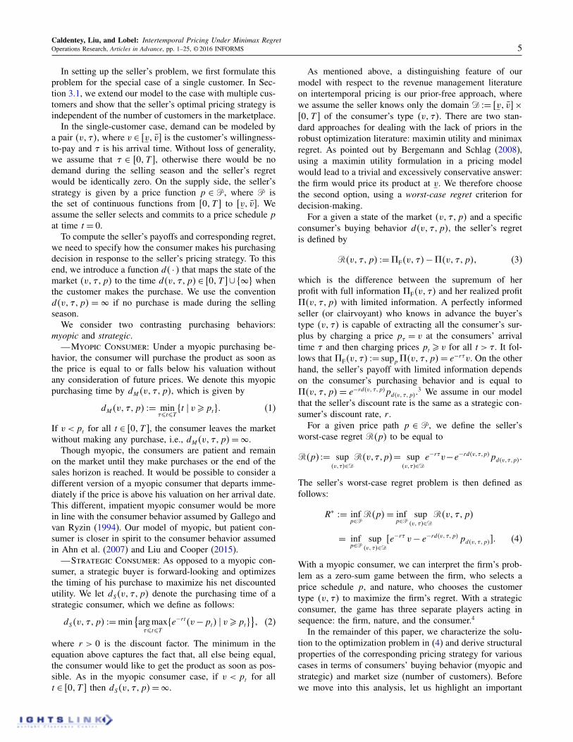
Figure 1. (Color online) Valuation and delay regretswith myopic customers.

Time period

Val

uatio

ns

T

v

v

Price path: pt

a

A

bB

db

vb

va

Valuationregret

Delay regret

0

pdb

p!a

!b !a

Hence, any type 4v1 í5 above the price path is dominated(in the sense of increasing the seller’s regret) by the type4v1 í5 in the upper boundary of the set D, which we denoteby D 2= 84v1 í5 2D2 v = v9. Consumers with type 4v1 í5

above the price path create valuation regret.Suppose now that nature picks consumer “b” whose type

(vb

1 í

b

5 is below the price path. In this case, the consumerdoes not buy immediately and must wait until time d

b

topurchase the product at price p

d

b

. In this case, the price pd

b

is equal to v

b

by the continuity of the price path. Hence, thecorresponding regret is equal to 4e

Érí

b É e

Érd

b

5v

b

. Again,nature can increase this regret to 41É e

Érd

b

5v

b

by choos-ing consumer “B” instead. This argument requires the pricepath p to be decreasing. It follows that any type 4v1 í5

below the price path is dominated by the type 4v105 inthe left boundary of the set D, which we denote by D0 2=84v1 í5 2 D2 í = 09. In this case, consumers with type4v1 í5 below the price path create delay regret.

At this point it should be intuitively clear that if the sellertries to reduce the valuation regret by increasing the pricepath then the delay regret will increase and vice versa. Asa result, an optimal price strategy must balance these twotypes of regrets as we show below.

Consider an arbitrary price path p 2P and let us evalu-ate its performance by looking at the valuation and delayregrets it generates. Based on our previous discussion amyopic customer can only generate one type of regretif the price path is continuous. Indeed, a consumer withtype 4v1 í5 generates the valuation regret eÉrí

4v É p

í

5 ifvæ p

í

or the delay regret 4eÉrí É e

Érd

M

4v1 í1p5

5v if v < p

í

.This delay regret includes the case in which the cus-tomer is priced out of the market (i.e., the price path8p

t

2 í ∂ t ∂ T 9 is strictly greater than v) since in this cased

M

4v1 í1 p5=à.With the previous decomposition of the regret in mind,

let us consider the set of functions p 2P that have a supre-mum (or worst-case) valuation regret that is less than or

equal to R, for some arbitrary R> 0. This is the set of func-tions p such that sup8eÉrí

4vÉp

í

5 ó 4v1 í5 2D9∂R. Sincethe argument inside the “sup” is monotonically increasingin v, we have the following result.

Lemma 1. Let us define p

t

4R5 2= 8v É e

rt

R9 _ v for all

t 2 601T 7. A function p 2 P has a worst-case valuation

regret that is bounded above by R if and only if it satisfies

the condition p

t

æ p

t

4R5 for all t 2 601T 70

Next, we would like to produce a similar result that char-acterizes the set of price paths that have a worst-case delayregret that is less than or equal to R. As we will see, we areable to produce such a result but with one caveat, namely,we have to restrict our characterization to the set of decreas-ing price paths in P. Fortunately, our next lemma showsthat this is not a serious limitation.

Lemma 2. For any price path p 2P there exists a decreas-

ing path p such that the seller’s worst-case regret under p

is less than or equal to the worst-case regret under p, that

is, RM4p5∂RM4p5.

We can now establish the following representation of theset of decreasing functions that have a worst-case delayregret bounded above by R.

Lemma 3. Let us define pt

4R5 2= 8v_R/41Ée

Ért

59^ v for

all t 2 601T 7. A decreasing function p 2P has a worst-case

delay regret that is bounded above by R if and only if it

satisfies the two conditions: (i) pt

∂ p

t

4R5 for all t 2 601T 7and (ii) p

T

∂R_ v.

The first inequality above captures the delay regret orig-inating from a customer delaying his purchase while thesecond one is associated with the risk of the consumer notpurchasing the firm’s product at all (which we represent asa delay until time t =à). Combining these three lemmas,we get the following proposition.

Proposition 2. A decreasing function p 2P has a worst-

case regret that is bounded above by R if and only if it

satisfies the conditions p

T

∂R_ v and p

t

4R5∂ p

t

∂ p

t

4R5

for all t 2 601T 7.

Equipped with this result, we can use a geometric argu-ment to derive the set of optimal price paths. Figure 2depicts three distinctive cases depending on the value of R.In the three panels, the dot at time t = T = 1 is located atthe level R_ v and is used the check the condition p

T

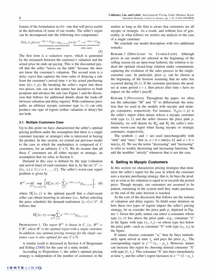
∂R_ v.Consider first the situation in panel (a). In this case the

value of R is sufficiently high so that pt

4R5< p

t

4R5 for allt 2 601T 7. It follows that any decreasing price path p 2Pinside the shaded area with p

T

∂ R_ v produces a worst-case regret that is bounded above by R.Starting from the situation in panel (a), the seller has

some room to reduce the value of the regret R. As shepushes R down, the function p

t

4R5 moves up and the func-tion p

t

4R5 moves down. However, if she overshoots in this

Dow

nloa

ded

from

info

rms.o

rg b

y [1

28.1

22.1

49.1

54] o

n 26

Janu

ary

2017

, at 1

8:23

. Fo

r per

sona

l use

onl

y, a

ll rig

hts r

eser

ved.

Caldentey, Liu, and Lobel: Intertemporal Pricing Under Minimax Regret8 Operations Research, Articles in Advance, pp. 1–25, © 2016 INFORMS

Figure 2. (Color online) (a) Feasible regret region, (b) infeasible regret region and (c) optimal regret regions.

0 10

0.2

1.0

0

0.2

1.0

0

0.2

1.0

(a) Feasible regret: R = 0.3

Pric

e

0 1

(b) Infeasible regret: R = 0.23

Time

0 1

(c) Optimal regret: R = 0.25

pt(R)

t* = ln(2)/r

pt(R)

pt(R)

pt(R) pt(R)

pt(R)

Notes. The decreasing dashed line represents the price path that, at each time point, equalizes the valuation regret for customers with v= v and the delayregret for customers with í = 0. The horizontal dashed line is located at the level v and the dot at time t = 1 is located at the level R_ v. Though withinthe optimal regret region, the decreasing dashed line in panel (c) is not actually optimal since it ends above the R_ v dot. Data: v = T = 1, v = 002,r = 102 and R= 003, R= 0023 and R= 0025 in panels (a)–(c), respectively.

process and decreases the value of R too much, she canfind herself in the situation depicted in panel (b). In thiscase, there is a region (shaded area) where p

t

4R5> p

t

4R5

and by Lemma 2 and Proposition 2 we know that there isno price path p 2P that can achieve a worst-case regret aslow as R.

From the results in panels (a) and (b), we conclude thatthe seller would like to push down the value of R as long asp

t

4R5∂ p

t

4R5 for all t 2 601T 7 and p

T

4R5∂ R_ v. As Rdecreases, one of these two constraints will be violated firstand will determine the optimal value of R. We can charac-terize the solution to the seller’s problem by studying whichconstraint is binding for a given set of problem parameters

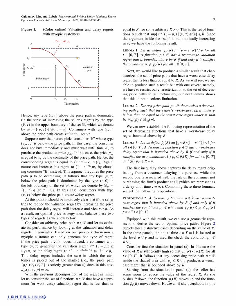
Figure 3. Parameter regions A1 to A4.

0 0.5 Log(3) 1.50

0.25

0.50

0.75

1.00

rT

u

A4

A3 A1

A2

and how precisely this constraint binds the optimizationproblem. To do so, we need to divide our parameter spaceinto four regions.The first region, which we denote by A1, is the one that

occurs if the time horizon T is long and the ratio u 2= v/v

is low. That is, there is a fair amount of uncertainty aboutthe consumer’s valuation and the firm has sufficient timeto dynamically change prices. For a precise definition ofthe four regions, including A1, see Figure 3. Panel (c) inFigure 2 represents the optimal region in the case wherethe problem parameters T and u belong to the region A1,though only paths within the optimal region that end atR_v or below are optimal. In this situation, the two curves

Dow

nloa

ded

from

info

rms.o

rg b

y [1

28.1

22.1

49.1

54] o

n 26

Janu

ary

2017

, at 1

8:23

. Fo

r per

sona

l use

onl

y, a

ll rig

hts r

eser

ved.

Caldentey, Liu, and Lobel: Intertemporal Pricing Under Minimax RegretOperations Research, Articles in Advance, pp. 1–25, © 2016 INFORMS 9

p

t

4R5 and p

t

4R5 intersect tangentially at a time t = t

⇤ with-out crossing. We call this time t

⇤ the critical time. Anydecreasing function p inside the shaded area with p

T

∂R_ v is an optimal price path. It is interesting to see thatin this situation every optimal price path p 2 P must gothrough the point at which p

t

4R5 and p

t

4R5 touch. We canderive the coordinates of this point as well as the optimalvalue of R by imposing the conditions:

p

t

⇤4R⇤M5= p

t

⇤4R⇤M5 and

ddt

p

t

4R

⇤M5

����t=t

⇤= d

dtp

t

4R

⇤M5

����t=t

⇤0

(7)

After some straightforward calculations, we get that

t

⇤= 1r

ln4251 p

t

⇤4R⇤M5= p

t

⇤4R⇤M5=

v

2and R

⇤M= v

40 (8)

Region A2 represents the case where the horizon T is stilllong, but the ratio u is large, i.e., there is not a lot ofmarket uncertainty. This region, with its long horizon T

and low market uncertainty, represents a best case scenariofor the firm. In this scenario, the binding constraint is stilla critical time t⇤ where the functions p

t

⇤4R⇤M5 and p

t

⇤4R⇤M5

intersect, except that they are no longer tangential at t⇤.Instead, what determines t

⇤ is the minimum valuation v.The minimax regret in region A2 can be determined bysolving the following pair of equations:

p

t

⇤4R⇤M5= p

t

⇤4R⇤M5= v0 (9)

With a bit of algebra, we can show that the regret in thisscenario is R⇤

M = u41É u5v.Regions A3 and A4 are associated with a short selling

horizon T . For these two regions, the binding constraintswitches to p

T

4R5 ∂ R _ v. That is, there is no time t

⇤

where the curves p

t

⇤4R⇤M5 and p

t

⇤4R⇤M5 intersect. Instead,

we call the end of the horizon T the critical time t

⇤ inregions A3 and A4. In region A3, the horizon T is shortand the ratio u is low (there is a lot of market uncer-tainty). Region A3 is thus the firm’s worst case scenario. Inthis scenario, the precise binding constraint is p

T

4R5∂ R,as the main risk facing the seller is the no purchase risk.Region A4 is characterized by a short T and a high u. Inthis case, the precise binding constraint is p

T

4R5∂ v. Per-haps counterintuitively, the seller’s regret is either insen-sitive to small changes in the discount rate r (regions A1

and A2), or is decreasing in r (regions A3 and A4). Inthe latter case, the seller’s regret decreases in r becausethe worst-case customer in A3 and A4 is one that arrivesat time T with valuation v. When r increases, the regretcaused by this customer time is reduced since it occurs attime T .

We are now ready to present the main result of this sec-tion, which synthesizes the discussion above.

Theorem 1 (Myopic Consumers). Letu= v/v. The seller’s

minimum worst-case regret is equal to

R

⇤M =

8>>>>>>>>>><

>>>>>>>>>>:

v

4if 4u1T 5 2A1

u41É u5v if 4u1T 5 2A2

v

1+ e

rT

if 4u1T 5 2A3

e

ÉrT

41É u5v if 4u1T 5 2A40

In addition, any decreasing pricing strategy p 2 P that

satisfies

p

T

∂R

⇤M _ v and

p

t

4R

⇤M5∂ p

t

∂ p

t

4R

⇤M5 for all t 2 601T 7

is optimal and generates a worst-case regret equal to R

⇤M.

It is not hard to see that the optimal regret R⇤M is non-

increasing in both T and u, implying that the seller is(weakly) better off if she increases the length of the sell-ing season or if she has less uncertainty about customer’svaluation.We conclude this section discussing the implications

of Theorem 1 on the seller’s choice of an optimal pricepath and duration of the selling season. However, beforeembarking on this practical discussion, we provide an addi-tional result that shows that our restriction to continuousdecreasing price paths is without loss of optimality.

Theorem 2. Let P be the set of functions from 601T 7 to6v1 v7 and let R

⇤M be the optimal regret in Theorem 1,

i.e., R

⇤M is the seller’s minimax regret within the set of

continuous price paths P. Then, the seller’s worst-case

regret under any p 2 P is bounded below by R

⇤M, that is

R

⇤M ∂RM4p5.

On the properties of optimal price paths. Possibly, oneof the most important insights of Theorem 1 is the factthat a price path that minimizes the maximum regret is notunique. The theorem also provides point-wise upper andlower bounds for the set of optimal price paths. Let usdenote by p

⇤t

2= p

t

4R

⇤M5 and p

⇤t

2= p

t

4R

⇤M5 the least upper

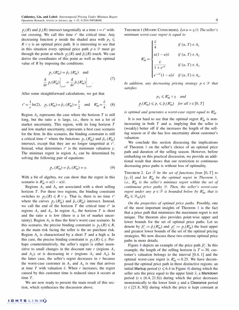
and greatest lower bounds of the set of the optimal pricingstrategies. We now discuss these two extreme optimal pricepaths in more details.Figure 4 depicts an example of the price path p

⇤t

. In thisexample, the length of the selling horizon is T = 30, cus-tomer’s valuation belongs to the interval 6004117 and theoptimal worst-case regret is R

⇤M = 0025. We have decom-

posed the optimal price path in three distinctive regions: aninitial Markup period (t ∂ 604 in Figure 4) during which theseller sets the price equal to the upper limit v, a Markdown

period (t 2 4604121085) during which the price decreasesmonotonically to the lower limit v and a Clearance period(t 2 621081307) during which the price is kept constant at

Dow

nloa

ded

from

info

rms.o

rg b

y [1

28.1

22.1

49.1

54] o

n 26

Janu

ary

2017

, at 1

8:23

. Fo

r per

sona

l use

onl

y, a

ll rig

hts r

eser

ved.

Caldentey, Liu, and Lobel: Intertemporal Pricing Under Minimax Regret10 Operations Research, Articles in Advance, pp. 1–25, © 2016 INFORMS

Figure 4. (Color online) Optimal price path p

⇤t

withv= 1, v= 004, T = 30, and r = 00045.

0 6.40 10.0 15.0 21.8 25.0 30.0

0.4

0.5

0.6

0.7

0.8

0.9

1.0

1.1

Time t

Pric

e

Markdown

Clearance

Markup

Note. In this example, R⇤M = 0025.

the lower limit v. The price path (and our choice of thenames for these three regions) resembles standard pricingpractice for seasonal or perishable products (see Bitran andCaldentey 2003 and references therein).

The presence of a Markup period in the optimal pathin Figure 4 is somehow counterintuitive since the seller iseffectively delaying sales until after this period. This fea-ture of an optimal price vector suggests that the seller’sworst-case regret R⇤

M is not affected by high markup pricesat the beginning of the selling season but rather by thechoices of prices during the Markdown and Clearance peri-ods. This idea is formalized in Theorem 1 that shows thatthe seller has a significant amount of flexibility in choos-ing prices before and after the critical time t

⇤, where t

⇤ isdefined as t

⇤2= min8min8t ó p⇤

t

= p

⇤t

91 T 9 (see panel (c)in Figure 2). Indeed, any decreasing price function p from601T 7 to 6v1 v7 is optimal if it is bounded above by p

⇤t

andbounded below by p

⇤t

and p4T 5∂R

⇤M _ v.

On the other hand, the price at time t⇤ is uniquely deter-mined. Interestingly, this result implies that the seller mustbe extremely careful in selecting the price at this time t

⇤

since her worst-case regret is defined by her pricing strat-egy at this point in time. To be more specific, whenever theselling horizon T is sufficiently long (regions A1 and A2),the seller’s regret is achieved when (i) a myopic customerwith valuation v = p

⇤t

⇤ = p

⇤t

⇤ arrives at the very beginningof the selling season and has to wait until the price is suf-ficiently low (at t

⇤) to make a purchase, or when (ii) amyopic customer with valuation v = v arrives at t

⇤ andbuys the product immediately. The seller’s optimal pricingstrategy in this myopic case is then designed to minimizethe regret associated with these two types of events.

The fact that the optimal price path is not unique raisesthe question of how to select a particular one. From the def-inition of the lower bound, we have p

⇤0 < v,5 that is, there

always exists an optimal price path with no Markup period.Hence, we can view the lower bound p

⇤t

as a conservativepricing option that charges low prices throughout the sell-ing season and, therefore, requires less markdowns. On the

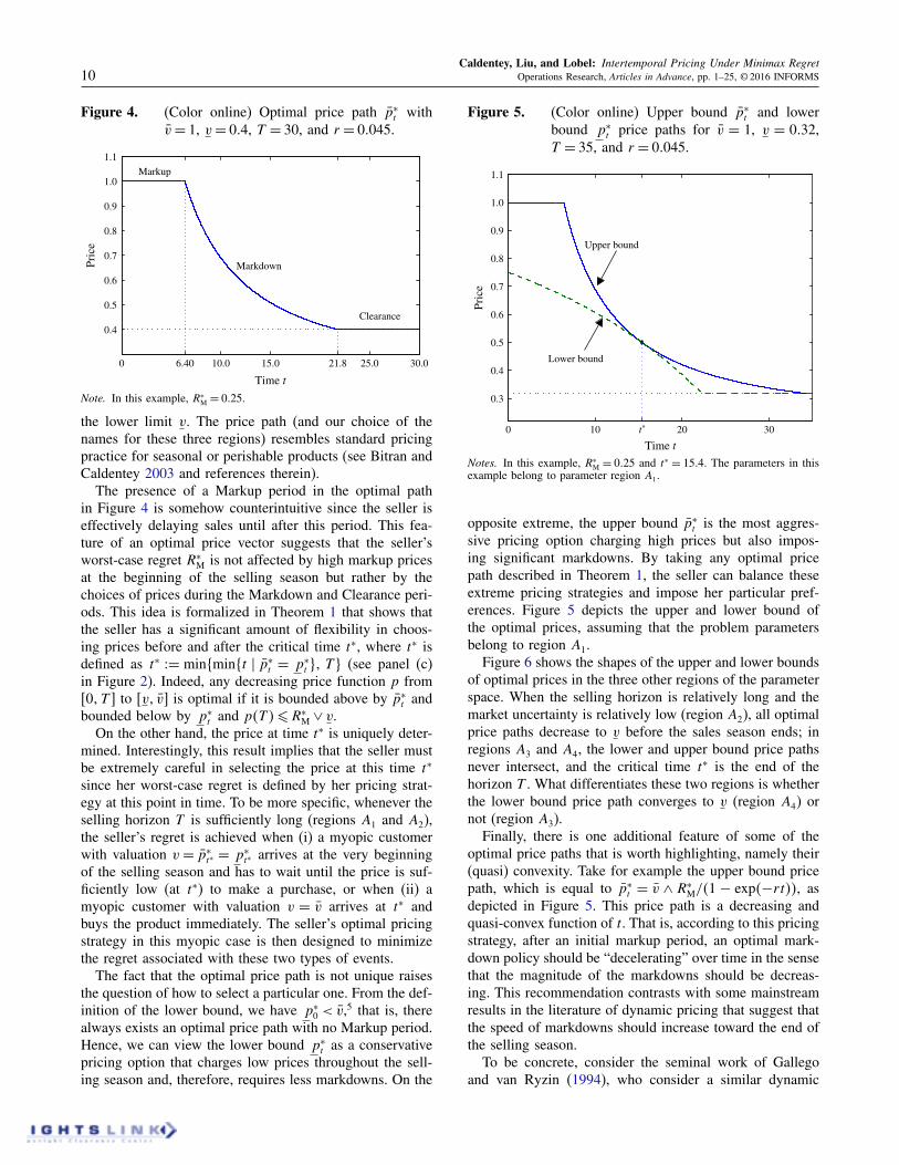
Figure 5. (Color online) Upper bound p

⇤t

and lowerbound p

⇤t

price paths for v = 1, v = 0032,T = 35, and r = 00045.

0 10 t* 20 30

0.3

0.4

0.5

0.6

0.7

0.8

0.9

1.0

1.1

Time t

Pric

e

Lower bound

Upper bound

Notes. In this example, R⇤M = 0025 and t

⇤ = 1504. The parameters in thisexample belong to parameter region A1.

opposite extreme, the upper bound p

⇤t

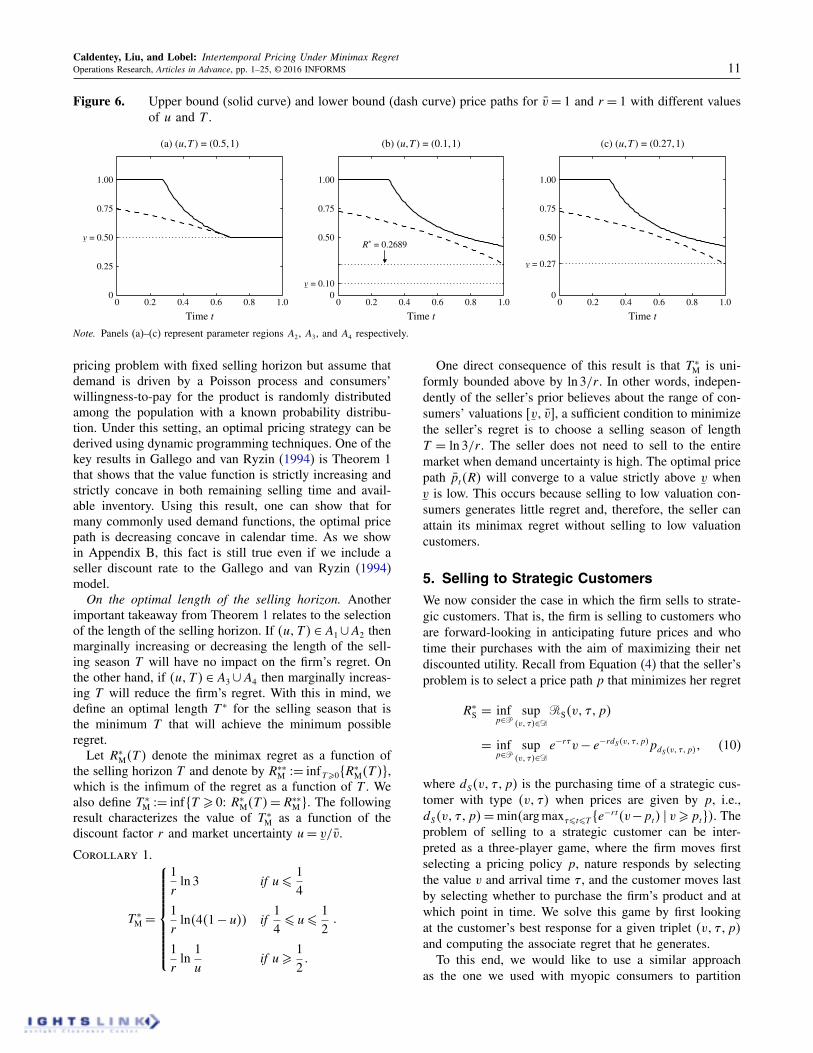
is the most aggres-sive pricing option charging high prices but also impos-ing significant markdowns. By taking any optimal pricepath described in Theorem 1, the seller can balance theseextreme pricing strategies and impose her particular pref-erences. Figure 5 depicts the upper and lower bound ofthe optimal prices, assuming that the problem parametersbelong to region A1.Figure 6 shows the shapes of the upper and lower bounds

of optimal prices in the three other regions of the parameterspace. When the selling horizon is relatively long and themarket uncertainty is relatively low (region A2), all optimalprice paths decrease to v before the sales season ends; inregions A3 and A4, the lower and upper bound price pathsnever intersect, and the critical time t

⇤ is the end of thehorizon T . What differentiates these two regions is whetherthe lower bound price path converges to v (region A4) ornot (region A3).Finally, there is one additional feature of some of the

optimal price paths that is worth highlighting, namely their(quasi) convexity. Take for example the upper bound pricepath, which is equal to p

⇤t

= v ^ R

⇤M/41 É exp4Ért55, as

depicted in Figure 5. This price path is a decreasing andquasi-convex function of t. That is, according to this pricingstrategy, after an initial markup period, an optimal mark-down policy should be “decelerating” over time in the sensethat the magnitude of the markdowns should be decreas-ing. This recommendation contrasts with some mainstreamresults in the literature of dynamic pricing that suggest thatthe speed of markdowns should increase toward the end ofthe selling season.To be concrete, consider the seminal work of Gallego

and van Ryzin (1994), who consider a similar dynamic

Dow

nloa

ded

from

info

rms.o

rg b

y [1

28.1

22.1

49.1

54] o

n 26

Janu

ary

2017

, at 1

8:23

. Fo

r per

sona

l use

onl

y, a

ll rig

hts r

eser

ved.

Caldentey, Liu, and Lobel: Intertemporal Pricing Under Minimax RegretOperations Research, Articles in Advance, pp. 1–25, © 2016 INFORMS 11

Figure 6. Upper bound (solid curve) and lower bound (dash curve) price paths for v= 1 and r = 1 with different valuesof u and T .

Time t0 0.2 0.4 0.6 0.8 1.0

Time t0 0.2 0.4 0.6 0.8 1.0

Time t0 0.2 0.4 0.6 0.8 1.0

0

0.25

v = 0.50

0.75

1.00

0

0.50

v = 0.10

0.75

1.00

v = 0.27

0

0.75

0.50

1.00

(a) (u,T ) = (0.5,1)

R* = 0.2689

(b) (u,T ) = (0.1,1) (c) (u,T ) = (0.27,1)

Note. Panels (a)–(c) represent parameter regions A2, A3, and A4 respectively.

pricing problem with fixed selling horizon but assume thatdemand is driven by a Poisson process and consumers’willingness-to-pay for the product is randomly distributedamong the population with a known probability distribu-tion. Under this setting, an optimal pricing strategy can bederived using dynamic programming techniques. One of thekey results in Gallego and van Ryzin (1994) is Theorem 1that shows that the value function is strictly increasing andstrictly concave in both remaining selling time and avail-able inventory. Using this result, one can show that formany commonly used demand functions, the optimal pricepath is decreasing concave in calendar time. As we showin Appendix B, this fact is still true even if we include aseller discount rate to the Gallego and van Ryzin (1994)model.

On the optimal length of the selling horizon. Anotherimportant takeaway from Theorem 1 relates to the selectionof the length of the selling horizon. If 4u1T 5 2A1[A2 thenmarginally increasing or decreasing the length of the sell-ing season T will have no impact on the firm’s regret. Onthe other hand, if 4u1T 5 2A3[A4 then marginally increas-ing T will reduce the firm’s regret. With this in mind, wedefine an optimal length T

⇤ for the selling season that isthe minimum T that will achieve the minimum possibleregret.

Let R⇤M4T 5 denote the minimax regret as a function of

the selling horizon T and denote by R

⇤⇤M 2= inf

Tæ08R⇤M4T 59,

which is the infimum of the regret as a function of T . Wealso define T

⇤M 2= inf8T æ 02 R⇤

M4T 5=R

⇤⇤M 9. The following

result characterizes the value of T

⇤M as a function of the

discount factor r and market uncertainty u= v/v.

Corollary 1.

T

⇤M =

8>>>>>>><

>>>>>>>:

1r

ln 3 if u∂ 14

1r

ln4441É u55 if

14∂ u∂ 1

2

1r

ln1u

if uæ 120

0

One direct consequence of this result is that T ⇤M is uni-

formly bounded above by ln 3/r . In other words, indepen-dently of the seller’s prior believes about the range of con-sumers’ valuations 6v1 v7, a sufficient condition to minimizethe seller’s regret is to choose a selling season of lengthT = ln 3/r . The seller does not need to sell to the entiremarket when demand uncertainty is high. The optimal pricepath p

t

4R5 will converge to a value strictly above v whenv is low. This occurs because selling to low valuation con-sumers generates little regret and, therefore, the seller canattain its minimax regret without selling to low valuationcustomers.

5. Selling to Strategic Customers

We now consider the case in which the firm sells to strate-gic customers. That is, the firm is selling to customers whoare forward-looking in anticipating future prices and whotime their purchases with the aim of maximizing their netdiscounted utility. Recall from Equation (4) that the seller’sproblem is to select a price path p that minimizes her regret

R

⇤S = inf

p2Psup

4v1 í52DRS4v1 í1p5

= infp2P

sup4v1 í52D

e

Érí

vÉ e

Érd

S

4v1 í1p5

p

d

S

4v1 í1p5

1 (10)

where d

S

4v1 í1p5 is the purchasing time of a strategic cus-tomer with type 4v1 í5 when prices are given by p, i.e.,d

S

4v1 í1p5=min4argmaxí∂t∂T

8e

Ért

4vÉp

t

5 ó væ p

t

95. Theproblem of selling to a strategic customer can be inter-preted as a three-player game, where the firm moves firstselecting a pricing policy p, nature responds by selectingthe value v and arrival time í , and the customer moves lastby selecting whether to purchase the firm’s product and atwhich point in time. We solve this game by first lookingat the customer’s best response for a given triplet 4v1 í1p5and computing the associate regret that he generates.To this end, we would like to use a similar approach

as the one we used with myopic consumers to partition

Dow

nloa

ded

from

info

rms.o

rg b

y [1

28.1

22.1

49.1

54] o

n 26

Janu

ary

2017

, at 1

8:23

. Fo

r per

sona

l use

onl

y, a

ll rig

hts r

eser

ved.

Caldentey, Liu, and Lobel: Intertemporal Pricing Under Minimax Regret12 Operations Research, Articles in Advance, pp. 1–25, © 2016 INFORMS

the space of consumers’ type D into those that generatevaluation regret and those that generate delay regret. How-ever, the strategic nature of consumers’ purchasing behav-ior makes this segmentation less useful for the purpose ofanalysis. A strategic consumer can generate simultaneouslyvaluation and delay regrets despite the continuity of theprice path since such a customer might wait if prices aredropping sufficiently fast. For this reason, it is not just thepath p but also its modulus of continuity that determinewhich customer types buy immediately at their arrival timeand which ones delay their purchase. To formalize this idea,we introduce the following definition.

Definition 1 (Threshold Valuations). For a given pricepath p 2 P let us define the real-extended functionp4p52 601T 7! 6v1à7 such that

p4p5

t

2= p

t

+ sups24t1T 7

⇢e

Érs

e

Ért É e

Érs

4p

t

Ép

s

5

+�0 (11)

For notational simplicity, we drop the dependence ofp4p5 on p. The threshold valuation function p

t

plays a pre-dominant role in characterizing strategic consumers’ pur-chasing behavior. Its importance lies on the following keyproperty: a strategic customer with type 4v1 í5 buys imme-diately at time í if and only if væ p

í

. Indeed, it is not hardto see that the condition

e

Érí

4vÉp

í

5æ e

Érs

4vÉp

s

5

+ for all s 2 4í1T 71

holds if and only if væ p

í

. As a result, we can view strate-gic customers as acting “myopically” with respect to p

instead of p, that is, they buy the product as soon as theirvaluations exceeds p. Using this property of p, it is possi-ble to draw a parallel with the case of myopic consumers toextrapolate the geometric method that we used to charac-terize optimal pricing strategies in the previous section (seeFigure 9 and the discussion that follows). However, thisline of attack is less effective in this case because work-ing with threshold valuation paths p

t

is more cumbersomethan working with price paths p

t

. The reason for this is thatthe set of continuous price paths P is “too large” in thiscase in sense that p is ill-defined at those times at whichp

t

is not differentiable. Hence, further restrictions on theset of price paths would be needed to develop a geomet-ric solution as we did in the myopic case. Instead of usingthis route, we tackle the seller’s minimum regret problemin (10) using a different approach consisting of the follow-ing two main steps. In the first step, we consider the specialcase in which nature is restricted to select consumers fromthe set D0 = 84v1 í5 2D2 í = 09, i.e., when all consumersare in the market at the beginning of the selling season.We solve this particular instance by adapting the machineryof mechanism design, and in particular the one on optimalscreening as in Mirrlees (1971) (see also Mussa and Rosen1978), to fit our robust minimax formulation. Then, in thesecond step, we show that if the seller uses the optimal

price path identified in the first step then nature will selectconsumers that arrive at time t = 0, i.e., from the set D0.As a result, we will be able to conclude that the proposedprice path is also optimal with respect to the larger set D.

5.1. Selling to Strategic Customers With Types in D0

We start the analysis outlined in the previous paragraph bylooking at the following special instance of problem (10):

R

⇤0 2= inf

p2Psup

4v1 í52D0

RS4v1 í1p5

= infp2P

supv∂v∂v

8vÉ e

Érd

S

4v101p5p

d

S

4v101p590 (12)

We use the subscript “0” to emphasize the fact that theregret R⇤

0 is calculated under the assumption that nature isrestricted to the set D0.To solve problem (12) we first look at the consumer’s

subproblem. Let U 4v1p5 be the maximum utility that aconsumer with valuation v 2 6v1 v7 arriving at time t = 0can get if the seller chooses the price path p 2P. That is,

U 4v1p5 2= max0∂t∂T

8e

Ért

4vÉp

t

5

+90

The positive part in the definition of U 4v1p5 captures theconsumer’s individual rationality constraint. That is, if v <min8p

t

2 0 ∂ t ∂ T 9 then the customer leaves the marketwithout buying the product and gets zero utility. To sim-plify our notation, let us introduce the following changeof variables: à 2= e

Ért and f 4à5 2= e

Ért

p

t

. It follows thatthe consumer’s utility maximization problem can be rewrit-ten as

U 4v1 f 5 2= maxà0∂à∂1

4àvÉ f 4à55

+1 (13)

where à0 2= e

ÉrT . In this formulation, the consumer actionis represented by à while the seller’s strategy is given bythe function f 4à5. Our requirement that price paths belongto P then translates to requiring that f 2 F , which is theset of continuous functions such that f 4à5/à 2 6v1 v7 for allà 2 6à0117. For a specific choice of f 2 F , the seller candivide the range of valuations 6v1 v7 into those that buy andthose that do not buy the product. Indeed, for a given f ,let us define

v

f

2= minà0∂à∂1

⇢f 4à5

à

�0 (14)

It follows that a consumer with valuation v 2 6v1 v

f

5 leavesthe market without buying while one with v 2 6v

f

1 v7 buysthe product and get a non-negative utility. Also, note thatfor any f 2F we have that v

f

2 6v1 v7.For a given f 2 F , and for a given consumer with val-

uation v 2 6v

f

1 v7, we can define the consumer’s optimalstrategy

à

f

4v5 2=max⇢argmaxà0∂à∂1

8àvÉ f 4à59

�for all v 2 6v

f

1 v70

The outer “max” in our definition of à

f

4v5 captures ourassumption that in case of indifference consumers prefer

Dow

nloa

ded

from

info

rms.o

rg b

y [1

28.1

22.1

49.1

54] o

n 26

Janu

ary

2017

, at 1

8:23

. Fo

r per

sona

l use

onl

y, a

ll rig

hts r

eser

ved.

Caldentey, Liu, and Lobel: Intertemporal Pricing Under Minimax RegretOperations Research, Articles in Advance, pp. 1–25, © 2016 INFORMS 13

to buy as early as possible. By the definition of v

f

inEquation (14), we have that U 4v

f

1 f 5= 0. Also, from con-vex analysis, we get the following useful properties aboutU 4v1 f 5 and à

f

4v5.

Lemma 4. Let f 2 F . The function U 4v1 f 5 is increasing

and convex in 6v1 v7. In addition, the maximizer à

f

4v5 is

right-continuous and nondecreasing in the interval 6v

f

1 v7.

Finally, for all v 2 6v

f

1 v7:

U 4v1 f 5=Z

v

v

f

à

f

4x5dx0

This lemma is often referred to in mechanism design asthe Envelope Theorem. From the definition of à

f

4v5 andthe previous lemma, we get that for all v 2 6v

f

1 v7

U 4v1 f 5= à

f

4v5vÉ f 4à

f

4v55=Z

v

v

f

à

f

4x5dx0 (15)

With this implicit derivation of the consumer’s utility andoptimal strategy, let us turn to the seller’s optimizationproblem and let us compute the regret generated by a cus-tomer with valuation v 2 6v1 v7. We identify two cases.

—Case 1: Suppose that v 2 6v1 v

f

5. Then, the customerleaves the market without buying and generates a regretequal to v.

—Case 2: Suppose that v 2 6v

f

1 v7. Then, the customerbuys the product and generates a regret equal to v Éf 4à

f

4v55. From Equation (15) we can rewrite this regret afollows Z

v

v

f

à

f

4x5dx+ v41É à

f

4v550

Combining Cases 1 and 2, we conclude that the seller’sminimum worst-case regret problem is given by

inff2F

R4f 5 where

R4f 5 2= v

f

⌧4vf

>v5_ maxv26v

f

1v7

⇢Zv

v

f

à

f

4x5dx+v41Éà

f

4v55

�0

The indicator ⌧4vf

> v5 is needed because Case 1 aboveonly happens if v

f

> v.Instead of solving the optimization above directly on the

set of functions f 2F we will use the function à

f

4x5 as ourdecision variable. We will then recover the value of f 4à5from the value of à using Equation (15). To proceed, notethat according to our definition of à

f

4x5 and to Lemma 4,we must restrict our attention to functions à4x5 in the fol-lowing set.

Definition 2. Let ‰4v5 be the set of right-continuous andnondecreasing functions à2 6v1 v7! 6à0117.

The following intermediate result plays a key role in ourderivation of an optimal solution.

Proposition 3. Let us fix v 2 6v1 v7 and consider the opti-

mization problem

R

v

2= v⌧4v > v5_ infà2‰4v5

maxv26v1v7

⇢Zv

v

à4x5dx+ v41É à4v55

�0

Then,

à

⇤4x5= à0 _ 41É ln4v5+ ln4x551 x 2 6v1 v71

is an optimal solution and

R

v

= v⌧4v > v5_ 4v+ v4ln4v5É ln4v5É 1551

where v 2=max8v1 v exp4à0 É 1590

Equipped with Proposition 3, we can now fully charac-terize the solution to the case in which nature is restrictedto the set D0. Essentially, this boils down to finding thevalue of the threshold v that minimizes R

v

. We can thenreverse our change of variables and transform an optimalstrategy in the à-space to an optimal strategy in the originalprice space. We summarize this derivation in the followingresult, which uses the following definition.

d

⇤4v5 2=É1

r

ln41É ln4v5+ ln4v55^ T 1 for all v 2 6v1 v70

Theorem 3. Suppose nature selects consumers from the

set D0 = 84v1 í5 2D2 í = 09. The value of v 2 6v1 v7 that

minimizes the regret R

v

in Proposition 3 is given by

v

⇤ =max⇢v1

v exp4eÉrT É 151+ e

ÉrT

�

and the seller’s minimax regret is equal to

R

⇤0 =R

v

⇤ = v

⇤ + v

⇤4ln4v5É ln4v⇤5É 151

where v

⇤2=max8v⇤1 v exp4eÉrT É 1590

An optimal pricing strategy for the seller is given by

p

⇤S4t5=

(e

rt

4vexp4eÉrtÉ15ÉR

⇤05 for all t2 601d⇤

4v

⇤57

v for all t24d⇤4v

⇤51T 70

As a result, a customer with valuation v 2 6v1 v

⇤5 leaves the

market without buying the product while one with valuation

v 2 6v

⇤1 v7 buys at time d

⇤4v5.

A few remarks about the result in Theorem 3 and prop-erties of an optimal price path are in order. First, the pricepath equalizes all regrets generated by customers with valu-ations above v⇤. Second, the optimal price path we find is aconvex and decreasing function of time. Actually, the pricepath is strictly deceasing until it reaches the lower boundv and then remains constant at this value. Whether or notthe price path reaches this lower bound during the sellingseason depends on the particular instance under consider-ation. To explore this issue in more detail, let us consider

Dow

nloa

ded

from

info

rms.o

rg b

y [1

28.1

22.1

49.1

54] o

n 26

Janu

ary

2017

, at 1

8:23

. Fo

r per

sona

l use

onl

y, a

ll rig

hts r

eser

ved.

Caldentey, Liu, and Lobel: Intertemporal Pricing Under Minimax Regret14 Operations Research, Articles in Advance, pp. 1–25, © 2016 INFORMS

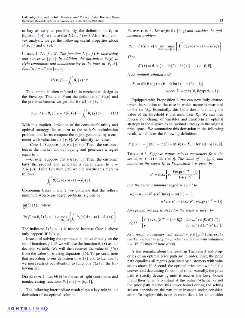
Figure 7. (Color online) Optimal price path p

⇤S4t5 and corresponding threshold valuation p

⇤S4t5 for different values of v.

pt: Threshold valuation

Panel (i): High market uncertainty Panel (ii): Medium market uncertainty Panel (iii): Low market uncertainty

pt: Price

v

0

0.3

1.0 1.0

1

Time0 1 0 1

˜pt: Threshold valuation˜ pt: Threshold valuation˜

pt: Price

pt: Price

0.4

1.0

0.6

v*˜

v*

Pric

e

v

v

v*˜

Notes. Data: v= T = 1, r = 102 and v= 003, v= 004 and v= 006 in panels (i)–(iii), respectively. Panels (i)–(iii) correspond to parameter regions B1, B2,and B3.

the numerical examples in Figure 7, which depicts the opti-mal price path p

⇤S4t5 and corresponding threshold valuation

p

⇤S4t5 introduced in Definition 1.We distinguish three different pricing regimes depending

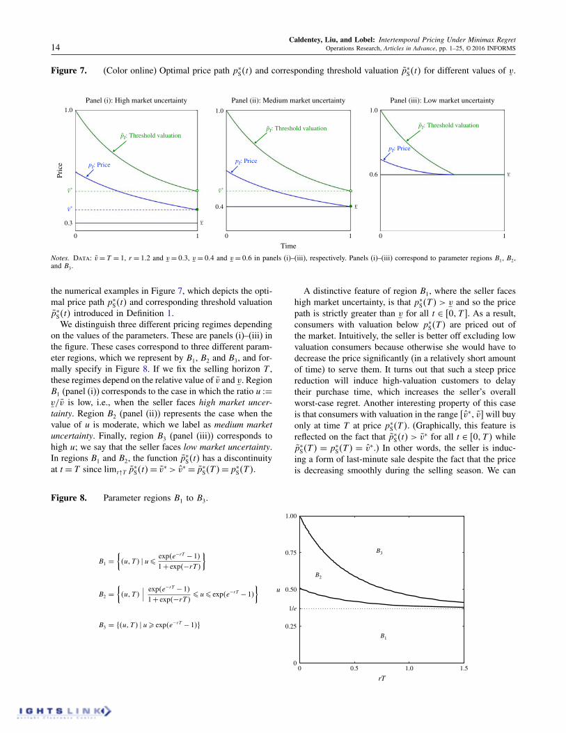
on the values of the parameters. These are panels (i)–(iii) inthe figure. These cases correspond to three different param-eter regions, which we represent by B1, B2 and B3, and for-mally specify in Figure 8. If we fix the selling horizon T ,these regimes depend on the relative value of v and v. RegionB1 (panel (i)) corresponds to the case in which the ratio u 2=v/v is low, i.e., when the seller faces high market uncer-tainty. Region B2 (panel (ii)) represents the case when thevalue of u is moderate, which we label as medium marketuncertainty. Finally, region B3 (panel (iii)) corresponds tohigh u; we say that the seller faces low market uncertainty.In regions B1 and B2, the function p

⇤S4t5 has a discontinuity

at t = T since limt"T p⇤

S4t5= v

⇤> v

⇤ = p

⇤S4T 5= p

⇤S4T 5.

Figure 8. Parameter regions B1 to B3.

0 0.5 1.0 1.50

0.25

1/e

0.50

0.75

1.00

rT

u

B1

B2

B3

A distinctive feature of region B1, where the seller faceshigh market uncertainty, is that p⇤

S4T 5 > v and so the pricepath is strictly greater than v for all t 2 601T 7. As a result,consumers with valuation below p

⇤S4T 5 are priced out of

the market. Intuitively, the seller is better off excluding lowvaluation consumers because otherwise she would have todecrease the price significantly (in a relatively short amountof time) to serve them. It turns out that such a steep pricereduction will induce high-valuation customers to delaytheir purchase time, which increases the seller’s overallworst-case regret. Another interesting property of this caseis that consumers with valuation in the range 6v⇤1 v7 will buyonly at time T at price p

⇤S4T 5. (Graphically, this feature is

reflected on the fact that p⇤S4t5 > v

⇤ for all t 2 601T 5 whilep

⇤S4T 5 = p

⇤S4T 5 = v

⇤.) In other words, the seller is induc-ing a form of last-minute sale despite the fact that the priceis decreasing smoothly during the selling season. We can

Dow

nloa

ded

from

info

rms.o

rg b

y [1

28.1

22.1

49.1

54] o

n 26

Janu

ary

2017

, at 1

8:23

. Fo

r per

sona

l use

onl

y, a

ll rig

hts r

eser

ved.

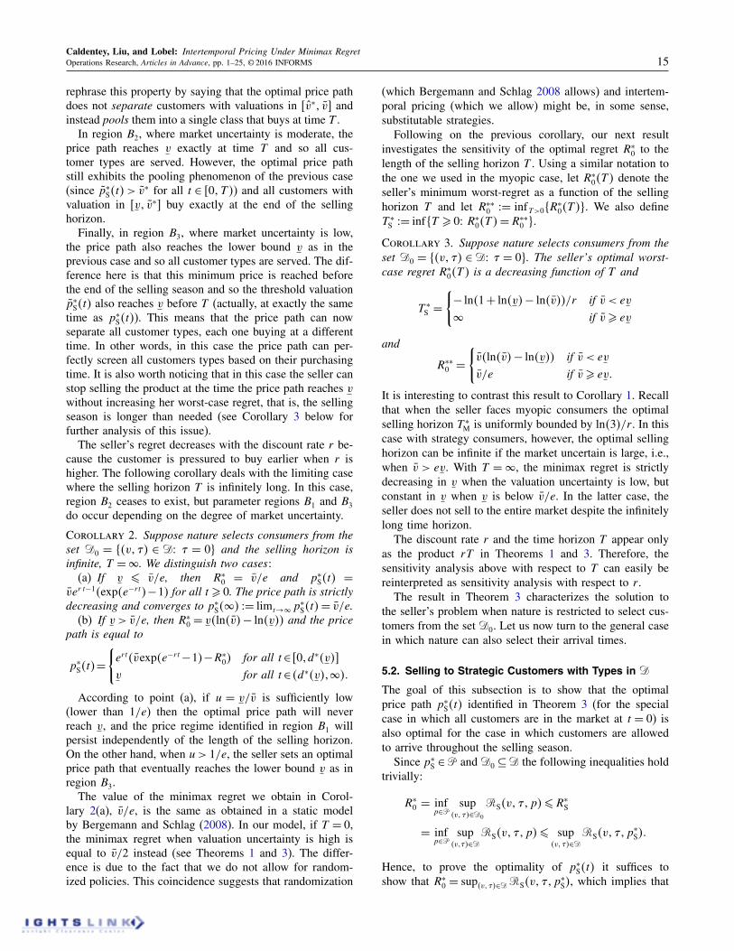
Caldentey, Liu, and Lobel: Intertemporal Pricing Under Minimax RegretOperations Research, Articles in Advance, pp. 1–25, © 2016 INFORMS 15

rephrase this property by saying that the optimal price pathdoes not separate customers with valuations in 6v

⇤1 v7 and

instead pools them into a single class that buys at time T .In region B2, where market uncertainty is moderate, the

price path reaches v exactly at time T and so all cus-tomer types are served. However, the optimal price pathstill exhibits the pooling phenomenon of the previous case(since p

⇤S4t5> v

⇤ for all t 2 601T 5) and all customers withvaluation in 6v1 v

⇤7 buy exactly at the end of the selling

horizon.Finally, in region B3, where market uncertainty is low,

the price path also reaches the lower bound v as in theprevious case and so all customer types are served. The dif-ference here is that this minimum price is reached beforethe end of the selling season and so the threshold valuationp

⇤S4t5 also reaches v before T (actually, at exactly the same

time as p

⇤S4t5). This means that the price path can now

separate all customer types, each one buying at a differenttime. In other words, in this case the price path can per-fectly screen all customers types based on their purchasingtime. It is also worth noticing that in this case the seller canstop selling the product at the time the price path reaches vwithout increasing her worst-case regret, that is, the sellingseason is longer than needed (see Corollary 3 below forfurther analysis of this issue).

The seller’s regret decreases with the discount rate r be-cause the customer is pressured to buy earlier when r ishigher. The following corollary deals with the limiting casewhere the selling horizon T is infinitely long. In this case,region B2 ceases to exist, but parameter regions B1 and B3do occur depending on the degree of market uncertainty.

Corollary 2. Suppose nature selects consumers from the

set D0 = 84v1 í5 2 D2 í = 09 and the selling horizon is

infinite, T =à. We distinguish two cases:

(a) If v ∂ v/e, then R

⇤0 = v/e and p

⇤S4t5 =

ve

r tÉ14exp4eÉrt

5É15 for all t æ 0. The price path is strictly

decreasing and converges to p

⇤S4à5 2= lim

t!à p

⇤S4t5= v/e.

(b) If v > v/e, then R

⇤0 = v4ln4v5É ln4v55 and the price

path is equal to

p

⇤S4t5=

(e

rt

4vexp4eÉrtÉ15ÉR

⇤05 for all t2 601d⇤

4v57

v for all t24d⇤4v51à50

According to point (a), if u = v/v is sufficiently low(lower than 1/e) then the optimal price path will neverreach v, and the price regime identified in region B1 willpersist independently of the length of the selling horizon.On the other hand, when u> 1/e, the seller sets an optimalprice path that eventually reaches the lower bound v as inregion B3.

The value of the minimax regret we obtain in Corol-lary 2(a), v/e, is the same as obtained in a static modelby Bergemann and Schlag (2008). In our model, if T = 0,the minimax regret when valuation uncertainty is high isequal to v/2 instead (see Theorems 1 and 3). The differ-ence is due to the fact that we do not allow for random-ized policies. This coincidence suggests that randomization

(which Bergemann and Schlag 2008 allows) and intertem-poral pricing (which we allow) might be, in some sense,substitutable strategies.Following on the previous corollary, our next result

investigates the sensitivity of the optimal regret R⇤0 to the

length of the selling horizon T . Using a similar notation tothe one we used in the myopic case, let R⇤

04T 5 denote theseller’s minimum worst-regret as a function of the sellinghorizon T and let R⇤⇤

0 2= infT>08R

⇤04T 59. We also define

T

⇤S 2= inf8T æ 02 R⇤

04T 5=R

⇤⇤0 9.

Corollary 3. Suppose nature selects consumers from the

set D0 = 84v1 í5 2D2 í = 09. The seller’s optimal worst-

case regret R

⇤04T 5 is a decreasing function of T and

T

⇤S =

(É ln41+ ln4v5É ln4v55/r if v < ev

à if væ ev

and

R

⇤⇤0 =

(v4ln4v5É ln4v55 if v < ev

v/e if væ ev0

It is interesting to contrast this result to Corollary 1. Recallthat when the seller faces myopic consumers the optimalselling horizon T

⇤M is uniformly bounded by ln435/r . In this

case with strategy consumers, however, the optimal sellinghorizon can be infinite if the market uncertain is large, i.e.,when v > ev. With T =à, the minimax regret is strictlydecreasing in v when the valuation uncertainty is low, butconstant in v when v is below v/e. In the latter case, theseller does not sell to the entire market despite the infinitelylong time horizon.The discount rate r and the time horizon T appear only

as the product rT in Theorems 1 and 3. Therefore, thesensitivity analysis above with respect to T can easily bereinterpreted as sensitivity analysis with respect to r .The result in Theorem 3 characterizes the solution to

the seller’s problem when nature is restricted to select cus-tomers from the set D0. Let us now turn to the general casein which nature can also select their arrival times.

5.2. Selling to Strategic Customers with Types in D

The goal of this subsection is to show that the optimalprice path p

⇤S4t5 identified in Theorem 3 (for the special

case in which all customers are in the market at t = 0) isalso optimal for the case in which customers are allowedto arrive throughout the selling season.Since p⇤

S 2P and D0 ✓D the following inequalities holdtrivially:

R

⇤0 = inf

p2Psup

4v1 í52D0

RS4v1 í1p5∂R

⇤S

= infp2P

sup4v1í52D

RS4v1 í1p5∂ sup4v1 í52D

RS4v1 í1p⇤S50

Hence, to prove the optimality of p

⇤S4t5 it suffices to

show that R⇤0 = sup

4v1 í52DRS4v1 í1p⇤S5, which implies that

Dow

nloa

ded

from

info

rms.o

rg b

y [1

28.1

22.1

49.1

54] o

n 26

Janu

ary

2017

, at 1

8:23

. Fo

r per

sona

l use

onl

y, a

ll rig

hts r

eser

ved.

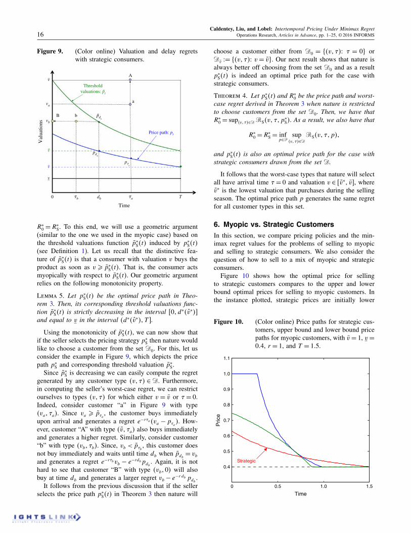
Caldentey, Liu, and Lobel: Intertemporal Pricing Under Minimax Regret16 Operations Research, Articles in Advance, pp. 1–25, © 2016 INFORMS

Figure 9. (Color online) Valuation and delay regretswith strategic consumers.

v

v

Val

uatio

ns

bB

A

a

Thresholdvaluations: pt

Price path: pt

v

v

vb

va

pdb

Time

Tdb0 !b !a

p!a

pdb

˜

˜

˜

R

⇤0 =R

⇤S. To this end, we will use a geometric argument

(similar to the one we used in the myopic case) based onthe threshold valuations function p

⇤S4t5 induced by p

⇤S4t5

(see Definition 1). Let us recall that the distinctive fea-ture of p⇤

S4t5 is that a consumer with valuation v buys theproduct as soon as v æ p

⇤S4t5. That is, the consumer acts

myopically with respect to p

⇤S4t5. Our geometric argument

relies on the following monotonicity property.

Lemma 5. Let p

⇤S4t5 be the optimal price path in Theo-

rem 3. Then, its corresponding threshold valuations func-

tion p

⇤S4t5 is strictly decreasing in the interval 601d⇤

4v

⇤57

and equal to v in the interval 4d

⇤4v

⇤51T 7.

Using the monotonicity of p⇤S4t5, we can now show that

if the seller selects the pricing strategy p⇤S then nature would

like to choose a customer from the set D0. For this, let usconsider the example in Figure 9, which depicts the pricepath p

⇤S and corresponding threshold valuation p

⇤S.

Since p

⇤S is decreasing we can easily compute the regret

generated by any customer type 4v1 í5 2 D. Furthermore,in computing the seller’s worst-case regret, we can restrictourselves to types 4v1 í5 for which either v = v or í = 0.Indeed, consider customer “a” in Figure 9 with type4v

a

1 í

a

5. Since v

a

æ p

í

a

, the customer buys immediatelyupon arrival and generates a regret eÉrí

a

4v

a

É p

í

a

5. How-ever, customer “A” with type 4v1 í

a

5 also buys immediatelyand generates a higher regret. Similarly, consider customer“b” with type 4v

b

1 í

b

5. Since, vb

< p

í

b

, this customer doesnot buy immediately and waits until time d

b

when p

d

b

= v

b

and generates a regret eÉrí

b

v

b

É e

Érd

b

p

d

b

. Again, it is nothard to see that customer “B” with type 4v

b

105 will alsobuy at time d

b

and generates a larger regret vb

É e

Ér d

b

p

d

b

.It follows from the previous discussion that if the seller

selects the price path p

⇤S4t5 in Theorem 3 then nature will

choose a customer either from D0 = 84v1 í52 í = 09 orD

v

2= 84v1 í52 v= v9. Our next result shows that nature isalways better off choosing from the set D0 and as a resultp

⇤S4t5 is indeed an optimal price path for the case with

strategic consumers.

Theorem 4. Let p⇤S4t5 and R

⇤0 be the price path and worst-

case regret derived in Theorem 3 when nature is restricted

to choose customers from the set D0. Then, we have that

R

⇤0 = sup

4v1 í52DRS4v1 í1p⇤S50 As a result, we also have that

R

⇤0 =R

⇤S = inf

p2Psup

4v1 í52DRS4v1 í1p51

and p

⇤S4t5 is also an optimal price path for the case with

strategic consumers drawn from the set D.

It follows that the worst-case types that nature will selectall have arrival time í = 0 and valuation v 2 6v

⇤1 v7, where

v

⇤ is the lowest valuation that purchases during the sellingseason. The optimal price path p generates the same regretfor all customer types in this set.

6. Myopic vs. Strategic Customers

In this section, we compare pricing policies and the min-imax regret values for the problems of selling to myopicand selling to strategic consumers. We also consider thequestion of how to sell to a mix of myopic and strategicconsumers.Figure 10 shows how the optimal price for selling

to strategic customers compares to the upper and lowerbound optimal prices for selling to myopic customers. Inthe instance plotted, strategic prices are initially lower

Figure 10. (Color online) Price paths for strategic cus-tomers, upper bound and lower bound pricepaths for myopic customers, with v= 1, v=004, r = 1, and T = 105.

0 0.5 1.0 1.5

0.4

0.5

0.6

0.7

0.8

0.9

1.0

1.1

Time

Pric

e

Strategic

Dow

nloa

ded

from

info

rms.o

rg b

y [1

28.1

22.1

49.1

54] o

n 26

Janu

ary

2017

, at 1

8:23

. Fo

r per

sona

l use

onl

y, a

ll rig

hts r

eser

ved.

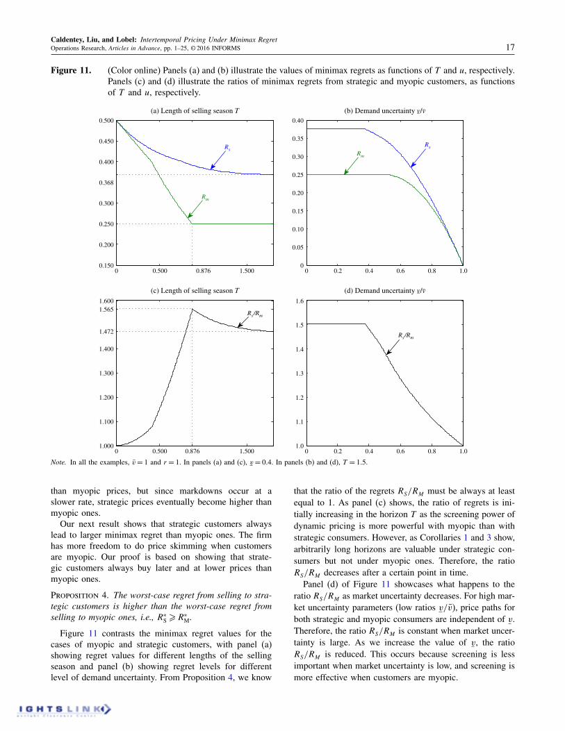
Caldentey, Liu, and Lobel: Intertemporal Pricing Under Minimax RegretOperations Research, Articles in Advance, pp. 1–25, © 2016 INFORMS 17

Figure 11. (Color online) Panels (a) and (b) illustrate the values of minimax regrets as functions of T and u, respectively.Panels (c) and (d) illustrate the ratios of minimax regrets from strategic and myopic customers, as functionsof T and u, respectively.

0 0.500 0.876 1.5000.150

0.200

0.250

0.300

0.368

0.400

0.450

0.500

(a) Length of selling season T

0 0.2 0.4 0.6 0.8 1.00

0.05

0.10

0.15

0.20

0.25

0.30

0.35

0.40

(b) Demand uncertainty v/v

0 0.500 0.876 1.5001.000

1.100

1.200

1.300

1.400

1.472

1.5651.600

(c) Length of selling season T

0 0.2 0.4 0.6 0.8 1.01.0

1.1

1.2

1.3

1.4

1.5

1.6

(d) Demand uncertainty v/v

Rs

Rm

Rs/Rm

Rs

Rm

Rs/Rm

Note. In all the examples, v= 1 and r = 1. In panels (a) and (c), v= 004. In panels (b) and (d), T = 105.

than myopic prices, but since markdowns occur at aslower rate, strategic prices eventually become higher thanmyopic ones.

Our next result shows that strategic customers alwayslead to larger minimax regret than myopic ones. The firmhas more freedom to do price skimming when customersare myopic. Our proof is based on showing that strate-gic customers always buy later and at lower prices thanmyopic ones.

Proposition 4. The worst-case regret from selling to stra-

tegic customers is higher than the worst-case regret from

selling to myopic ones, i.e., R

⇤S æR

⇤M.

Figure 11 contrasts the minimax regret values for thecases of myopic and strategic customers, with panel (a)showing regret values for different lengths of the sellingseason and panel (b) showing regret levels for differentlevel of demand uncertainty. From Proposition 4, we know

that the ratio of the regrets RS

/R

M

must be always at leastequal to 1. As panel (c) shows, the ratio of regrets is ini-tially increasing in the horizon T as the screening power ofdynamic pricing is more powerful with myopic than withstrategic consumers. However, as Corollaries 1 and 3 show,arbitrarily long horizons are valuable under strategic con-sumers but not under myopic ones. Therefore, the ratioR

S

/R

M

decreases after a certain point in time.Panel (d) of Figure 11 showcases what happens to the

ratio R

S

/R

M

as market uncertainty decreases. For high mar-ket uncertainty parameters (low ratios v/v), price paths forboth strategic and myopic consumers are independent of v.Therefore, the ratio R

S

/R

M

is constant when market uncer-tainty is large. As we increase the value of v, the ratioR

S

/R

M

is reduced. This occurs because screening is lessimportant when market uncertainty is low, and screening ismore effective when customers are myopic.

Dow

nloa

ded

from

info

rms.o

rg b

y [1

28.1

22.1

49.1

54] o

n 26

Janu

ary

2017

, at 1

8:23

. Fo

r per

sona

l use

onl

y, a

ll rig

hts r

eser

ved.

Caldentey, Liu, and Lobel: Intertemporal Pricing Under Minimax Regret18 Operations Research, Articles in Advance, pp. 1–25, © 2016 INFORMS

6.1. Mix of Myopic and Strategic Consumers

So far, we have assumed that there is a single type of con-sumers (myopic or strategic) in the market and that theseller knows the consumer type. In this subsection, we con-sider what happens if both types are present in the mar-ket simultaneously, and the fraction of consumers that arestrategic is unknown to the seller. Results in Su (2007) andMersereau and Zhang (2012) suggest that the structure ofan optimal pricing strategy might be sensitive to the propor-tions of myopic and strategic consumers in the marketplace.To capture this type of market heterogeneity, in this sec-tion we extend our robust formulation by allowing natureto select the mix of myopic and strategic consumers.

Let us consider first the case of a single consumer. In thisnew setting, the type of this consumer is a triplet 4v1 í1 à5,where v 2 6v1 v7 is his valuation, í 2 601T 7 is his arrivaltime and à 2 8M1S9 is his purchasing behavior, where “M”stands for myopic and “S” for strategic. We define the set ofthe consumers’ types to be D

‰

2= 6v1 v7⇥ 601T 7⇥ 8M1S9.We also define the projections D

M

2=D‰

\ 8à =M9 andD

S

2=D‰

\ 8à = S9, corresponding to the cases when allconsumers are myopic or strategic, respectively.

Depending on whether nature can select a consumer’stype from the set D

‰

, DM

or DS

, the seller’s minimaxregret is given by

R

⇤j

2= minpæ0

max4v1 í1 à52D

j

R4v1 í1 à1p5

= minpæ0

max4v1 í1 à52D

j

e

Érí

vÉ e

Érd4v1 í1 à1p5

p

d4v1 í1 à1p5

for j =‰1M1S1

where d4v1 í1 à1p5 is the purchasing time of a 4v1 í1 à5-consumer that faces the price path p 2P. We also denoteby p

⇤j

an optimal price path for j =‰1M1S.According to Proposition 4, we know that R

⇤S

æ R

⇤M

.Also, since D

S

✓ D‰

, we also have that R⇤‰

æ R

⇤S

. As aresult, we can rank the seller’s minimax regrets as followsR

⇤‰

æR

⇤S

æR

⇤M

. The next result shows that the first inequal-ity is indeed an equality. That is, even if nature is able toselect consumers’ types from D

‰

, the seller can achieve thesame minimax regret as if nature was restricted to selecttypes from the set of strategic consumers D

S

.

Proposition 5. Suppose nature can select the buyer’s type

from the set D‰

. Then, an optimal pricing strategy for the

seller is to select the vector p

⇤‰

= p

⇤S

identified in Theo-

rem 3. As a result, R

⇤‰

=R

⇤S

.

Suppose now that instead of a single buyer, the marketis populated by C æ 1 consumers and nature is capable ofselecting the proportion of myopic and strategic consumers.Let us denote by R

⇤C‰

, the seller’s minimax regret. The fol-lowing result extends Proposition 1 to this setting.

Proposition 6. The regret R

⇤C‰

is linear in C, i.e., R

⇤C‰

=CR

⇤‰

, where R

⇤‰

is the optimal regret with a single customer.

In addition, any optimal pricing strategy for the single cus-

tomer case is also optimal for any C 2�. We conclude fromProposition 5 that p

⇤S

(an optimal price vector when there

is a single strategic consumer in the market) is optimal.

In summary, the previous result reveals that if the selleris uncertain about the types of consumers in the market thenher best strategy is to use the same pricing policy that shewould use if she knew that all consumers were strategic.

7. Time-Dependent Valuations

The robust formulation presented in the previous sectionsassumes that customers’ valuations are independent of timein the sense that nature is allowed to select customers’ typesfrom the rectangle D = 6v1 v7⇥ 601T 7. In many practicalsituations, however, we can expect some degree of corre-lation between a customer’s arrival time and his valuation.To capture this correlation between arrival times and valu-ations, in this section, we consider the case in which natureis restricted to select customer’s types from a set D✓D. Inparticular, we will assume that there exist two continuousfunctions v

t

and v

t

with v∂ v

t

∂ v

t

∂ v and such that

D 2= 84v1 í5 2D2 0∂ í ∂ T and v

í

∂ v∂ v

í

90 (16)

In other words, we will consider sets D for which cus-tomers’ valuations belong to an interval that can changeover the selling season. For example, customers arrivingat the begin of the season could have higher valuationsfor the product than late-comers (e.g., as in the fashion orhigh-tech industries where products exhibit high degree ofobsolescence). To model this situation we could consider aset D as in Equation (16) for which the upper level of therange of valuations, v

t

, is a decreasing function of time.Interestingly, in what follows we show that under some

mild conditions on the set D this generalization does notchange the structure of our proposed solutions. Let us firstconsider the case of myopic customers. In this case, thegeometric argument that we used in Section 4 to decom-pose the seller’s regret into valuation and delay regrets stillholds. As a result, we can import the same solution methodto derive the following result.

Proposition 7. Suppose customers are myopic and nature

is restricted to choose types from a set D as in Equa-

tion (16) such that D0 ✓ D. Then, a decreasing function

p 2P has a worst-case regret that is bounded above by R

if and only if it satisfies the conditions p

T

∂R_ v and

p

t

4R5 2= 8v

t

Ée

rt

R9_v

t

∂ p

t

∂⇢v

t

_ R

1Ée

Ért

�^ v

t

=2

ˆp

t

4R5 for all t2 601T 70

Furthermore, the minimum worst-case regret R

⇤is the mini-

mum value of R for which the conditions (i) p

t

4R5∂ ˆp

t

4R5

for all t 2 601T 7 and (ii) p

T

4R5 ∂ R _ v are satisfied.

Any decreasing price path p

t

that satisfies p

t

4R

⇤5∂ p

t

∂ˆp

t

4R

⇤5 and p

T

4R5∂R_ v for all t 2 601T 7 is optimal.

Dow

nloa

ded

from

info

rms.o

rg b

y [1

28.1

22.1

49.1

54] o

n 26

Janu

ary

2017

, at 1

8:23

. Fo

r per

sona

l use

onl

y, a

ll rig

hts r

eser

ved.

Caldentey, Liu, and Lobel: Intertemporal Pricing Under Minimax RegretOperations Research, Articles in Advance, pp. 1–25, © 2016 INFORMS 19

Let us turn now to the case of strategic consumers.

Proposition 8. Suppose customers are strategic and na-

ture is restricted to choose types from a set D as in Equa-

tion (16) such that D0 ✓ D. Then, the optimal solution

identified in Theorem 3 is still optimal.

It is worth noticing that this result generalizes to an arbi-trary set D—not necessary of the form in Equation (16)—as long as D0 ✓ D. Intuitively, this result highlights a dis-tinctive feature of the case with strategic customers, namelythat an optimal price path is one that protects the selleragainst the event of a consumer arriving at the very begin-ning of the selling season, i.e., a customer with type in D0.Hence, as long as the set D includes D0, the solution inTheorem 3 is optimal. The condition D0 ✓ D seems reason-able in many practical settings, specially in those in whichconsumers’ valuations tend to decrease over time.

8. Concluding Remarks

In this paper we have investigated the intertemporal pricingproblem faced by a monopolist selling to myopic and/orstrategic customers over a finite selling horizon. A dis-tinctive feature of our work is that we have endowed theseller with a minimal amount of information about marketdemand. In particular, we have assumed that the seller onlyknows the range of customers’ valuations and has no priorbelief on how these valuations are distributed on this rangeor how customers arrive over the selling season. In thisdistribution-free environment, we tackle the seller’s pricingproblem using a robust minimax formulation in which theseller selects a price path that minimizes her worst-caseregret, that is, the difference between her payoff under fulldemand information and her realized payoff.

With myopic customers, we show that the seller’s regretadmits a decomposition in terms of delay and valuationregrets. Delay regret occurs when a low-valuation cus-tomer arrives early in the selling season and must wait forthe price to drop below his valuation level before he canpurchase the product. On the other hand, valuation regretoccurs when a high-valuation customer buys the productimmediately upon arrival. These two types of regrets act asopposing forces that the seller must balance at optimality.Using a geometric argument we show how to solve thistrade-off and how to characterize an optimal pricing strat-egy. Furthermore, we show that an optimal price path isnot unique and we provide (point-wise) upper and lowerbounds for the set of optimal price paths. We also showthat a representative price strategy consists of three distinctphases: an initial markup, a markdown, and a final clear-ance phase. Our analysis also reveals that despite of themultiplicity of optimal price paths they all coincide at aparticular critical time. In other words, while the seller hasflexibility to set prices in early and late stages of the sellingseason, she is restricted in her pricing decision around thisparticular point in time. Another interesting feature when

selling to myopic customers is that the optimal length ofthe selling season is uniformly bounded, independently ofthe range of customers’ valuations.With strategic customers, the geometric argument that we

use to solve the myopic case is less effective since strategiccustomers can simultaneously generate delay and valuationregrets. As a result, we use a different approach to solve theseller’s problem. In particular, we view the seller’s pricingproblem as a screening problem and adapt the machinery ofmechanism design to fit our robust minimax formulation.Our analysis shows that—depending on the parameters ofthe model—there exist three types of pricing regimes. First,when the seller faces significant demand uncertainty (i.e.,when the range of customers’ valuations is wide), it is opti-mal to set a price path that leaves low-valuation consumersout of the market. On the other hand, for moderate (or inter-mediate) levels of demand uncertainty, the seller selects aprice path that serves every customer type. However, low-valuation consumers are pooled together into a single classthat buys the product exactly at the end of the selling sea-son. Finally, when demand uncertainty is low, the sellersets a price path that not only serves every customer typebut also separates them based on their purchasing time, i.e.,the pricing strategy behaves as a prefect screening device.In general, compared to the myopic case, an optimal pricepath is “flatter” in the sense that the optimal price pathrelies less on markdowns. Also, it is no longer true thatthere is a uniform upper bound on the length of the sellingseason. That is, with strategic customers, it is possible thatthe seller wants to extend the selling season indefinitely.There are many interesting questions that we leave open

for future research. Intertemporal pricing under minimaxregret without commitment is a topic that we do not addressin our paper. Another such question is whether a random-ized pricing policy could be used to further reduce theseller’s regret. A further interesting follow-up project wouldbe to incorporate inventory into our model. Inventory con-siderations are an important factor in practice, but, as Cor-rea et al. (2016) show, they generally lead to a multiplicityof equilibria in settings with strategic customers. Allowingconsumers to exit the market without purchasing before theend of the sales horizon, for either endogenous or exoge-nous reasons, would also be an interesting extension to con-sider. Extending our methodology to more complex uncer-tainty sets than intervals over the customers’ valuations orto consider different demand classes with different uncer-tainty sets would also be valuable extensions, Section 7above constitutes a first step in this direction.

Acknowledgments

The authors thank Chung-Piaw Teo, the associate editor and thetwo referees for their thoughtful recommendations. The paperbenefited greatly from their suggestions.

Dow

nloa

ded

from

info

rms.o

rg b

y [1

28.1

22.1

49.1

54] o

n 26

Janu

ary

2017

, at 1

8:23

. Fo

r per

sona

l use

onl

y, a

ll rig

hts r

eser

ved.

Caldentey, Liu, and Lobel: Intertemporal Pricing Under Minimax Regret20 Operations Research, Articles in Advance, pp. 1–25, © 2016 INFORMS

Appendix A. Proofs

Proof of Proposition 1. Consider the seller’s optimal regret R⇤C

in (6). A lower bound of this regret is obtained by restrictingnature’s optimization to the subset DC

0 ✓ DC such that 8v1 í9 2DC

0 if and only if v1 = v2 = · · · = v

C

and í1 = í2 = · · · = í

C

, thatis, all C customers have identical valuations and arrival times.But if all customers are identical then the seller’s regret is equalto C times the optimal regret with a single customer, that is,R

⇤C æCR

⇤.On the other hand, any fixed pricing strategy p

t

leads to anupper bound for R⇤C in the sense that

R

⇤C ∂ sup8v1 í92DC

Á

C

F

4v1 í5ÉCX

i=1

e

Érd4v

i

1 í

i

1p5

p

d4v

i

1 í

i

1p5

�0

Furthermore, it is not hard to see that

Á

C

F

4v1 í5∂CX

i=1

e

Érí

i

v

i

since the right-hand side is the payoff that a clairvoyant can getunder perfect price discrimination (i.e., charging a different priceto every customer). It follows that

R

⇤C ∂ sup8v1 í92DC

CX

i=1

e

Érí

i

v

i

É e

Érd4v

i

1 í

i

1p5

p

d4v

i

1 í

i

1p5

�

=CX

i=1

sup8v

i

1 í

i

92D

e

Érí

i

v

i

É e

Érd4v

i

1 í

i

1p5

p

d4v

i

1 í

i

1p5

�1

hence the maximization above decouples for every customer. Butif the seller selects a pricing vector p⇤

t

, which is an optimal pric-ing strategy for the case of single customer, then each term inthe summation on the right equals R

⇤, that is, R⇤C ∂ CR

⇤. Weconclude that R⇤C =CR

⇤. É

Proof of Lemma 1. Consider a price path p

t

such that p

t

æp

t

4R5 for all t 2 601T 70 The worst-case valuation regret from p

t

satisfies the following inequality

maxt

e

Ért

4vÉp

t

5 ∂ maxt

e

Ért

4vÉ p

t

4R55

∂ maxt

e

Ért

4vÉ 4vÉ e

rt

R55=R0 É

Proof of Lemma 2. Consider an arbitrary price path p 2P (i.e.,a continuous function from 601T 7 to 6v1 v7) and let

RM4p5 = sup4v1 í52D

RM4v1 í1p5

= sup4v1 í52D

8e

Érí

vÉ e

Érd

M

4v1 í1p5

p

d

M

4v1 í1p5

91

be the corresponding seller’s worst-case regret. In what follows,we show that there always exists a (weakly decreasing) price pathp such that RM4p5∂RM4p5.

Indeed, for a given p 2 P, we let p be the running minimumprice path induced by p that is given by p

t

2=min8pí

2 í 2 601 t79for t 2 601T 7 (the “min” is well-defined by the continuity of p andWeierstrass Theorem). By construction, p is (weakly) decreasingand continuous (since p is continuous). To show that RM4p5 æRM4p5 let us partition the customer type’s space D into the fol-lowing three subsets D1 2= 84v1 í5 2D2 p

í

∂ v9, D2 2= 84v1 í5 2D2 p

í

∂ v < p

í

9 and D3 2= 84v1 í5 2 D2 p

í

> v9 and define

R

i

4p5 2= sup4v1 í52D

i

RM4v1 í1p5. In what follows, we show thatR

i

4p5=R

i

4p5 for i= 113 and that R24p5∂R14p5. As a result,

RM4p5 = maxi=11213

8R

i

4p59æmaxi=113

8R

i

4p59=maxi=113

8R

i

4p59

= maxi=11213

8R

i

4p59=RM4p50

—Let 4v1 í5 2 D1. By the definition of p, there exists at ∂ í such that p4t5 = p4t5 ∂ p4í5 ∂ v. Since consumers aremyopic, it follows thatRM4v1 t1p5=RM4v1 t1 p5= e

Ért

4vÉp

t

5æRM4v1 í1p5. Since 4v1 t5 2D1, we conclude that R14p5=R14p5.

—Let 4v1 í5 2 D3. In this case, it is easy to see thatd

M

4v1 í1p5 = d

M

4v1 í1 p5 (possibly à) and p4d

M

4v1 í1p55 =p4d

M

4v1 í1 p5. It follows that RM4v1 í1p5 = RM4v1 í1 p5. Weconclude that R34p5=R34p5.

—Let 4v1 í5 2D2. Since p

í

> p

í

there exists a t 2 601 í5 suchthat p4t5= p4t5∂ v. It follows that RM4v1 í1 p5= e

Érí

4vÉ p

í

5∂e

Ért

4v É p

t

5 = RM4v1 t1 p5. Furthermore, 4v1 t5 2 D1. Hence,R24p5∂R14p5.

It follows from the three cases above that RM4p5 æ RM4p5.Hence, without loss of optimality the seller can restrict attentionto (weakly) decreasing price functions. É

Proof of Lemma 3. Let p 2P be a decreasing function. For anycustomer type 4v1 í5 with v < p

í

, the delay regret he generates isequal to 4e

Érí É e

Érd

M

4v1 í1p5

5v. We distinguish two cases:—Case 1: d

M

4v1 í1 p5∂ T . In this case the customer buys theproduct at a future time d

M

4v1 í1 p5 such that pd

M

4v1 í1p5

= v andhe generates a delay regret 4eÉrí É e

Érd

M

4v1 í1p5

5p

d

M

4v1 í1p5

that isbounded above by 41Ée

Érd

M

4v1 í1p5

5p

d

M

4v1 í1p5

. But, by hypothesis,the price path p satisfies p

t

∂ R/41É e

Ért

5_ v for all t 2 601T 7.Furthermore, from the monotonicity of p and the fact that v < p

í

it is not hard to see that R/41 É e

Érd

M

4v1 í1p5

5 æ v. As a result,41Ée

Érd

M

4v1 í1p5

5p

d

M

4v1 í1p5

∂R, that is, the delay regret generatedby the customer is less than or equal to R.

—Case 2: dM

4v1 í1p5=à. In this case the customer is pricedout of the market. Since p is a decreasing price path this meansthat v < p

T

. But, by hypothesis, pT

∂ R_ v, hence this case canonly occur if R > v. So, assuming R > v, the delay regret inthis case is equal to e

Érí

v, which is bounded above by v, whichtogether with the inequalities v < p

T

< R imply that the delayregret generated by the customer is less than R. É

Proof of Proposition 2. This result follows immediately fromLemmas 1–3. É

Proof of Theorem 1. Proposition 2 characterizes the set of min-imax regret price paths. Region A1 is the set of problem param-eters where the solution is given by the price paths p

t

4R5 andp

t

4R5 intersecting tangentially as described by Equations (7) and(8). For this solution to be feasible, the ratio u= v/v must satisfyu∂ 1/2 to ensure the middle equation of (8) is feasible. The solu-tion must also satisfy p

t

4R5= vÉ e

rT

R∂ R_ v, where R= v/4from the right-most equation in (8). Therefore, A1 is character-ized by

u∂ 12

and T æmin⇢ln 3r

1

ln4441É u55

r

�0

In regions A2, A3, and A4, the boundary conditions (u and/or T )become binding and, thus, play a role in determining the mini-max regret. If uæ 1

2 and the selling horizon is sufficiently long,the binding constraint becomes p

t

⇤4R⇤M5= p

t

⇤4R⇤M5= v for some

Dow

nloa

ded

from

info

rms.o

rg b

y [1

28.1

22.1

49.1

54] o

n 26

Janu

ary

2017

, at 1

8:23

. Fo

r per

sona

l use

onl

y, a

ll rig

hts r

eser

ved.

Caldentey, Liu, and Lobel: Intertemporal Pricing Under Minimax RegretOperations Research, Articles in Advance, pp. 1–25, © 2016 INFORMS 21

t

⇤, as given by Equation (9). We can solve for R

⇤M and t

⇤ toget R⇤

M = u41É u5v and t

⇤ = 41/r5 ln41/u5. Thus, we need T æ41/r5 ln41/u5 to guarantee to obtain t

⇤ ∂ T . The pair of conditionsuæ 1

2 and T æ 41/r5 ln41/u5 lead to the definition of A2.In the regime where 4u1T 5 y A1 [ A2, the binding constraint

becomes p

T

4R

⇤M5=max8R⇤

M1 v9. One can solve the equation

vÉ e

rt

R

⇤M =max8R⇤

M1 v9 (A1)

and get the following results: if T ∂min8ln435/r1 ln41/uÉ15/r9,then the value that maximizes the right-hand side of Equa-tion (A1) is R⇤

M, generating the solution associated with region A3;otherwise, the right-hand side of Equation (A1) is maximizedby v, producing the solution for region A4. ÉProof of Theorem 2. Consider an arbitrary price path p withregret RM4p5 and let us suppose that RM4p5<R

⇤M. In what fol-

lows, we will show that the previous inequality leads to a contra-diction. For this, consider the critical time t

⇤ (see the discussionthat precedes Theorem 1). It is not hard to see that the lowerbound p

t

4R

⇤M5 is strictly decreasing in 601 t⇤7. It follows, under

the assumption that RM4p5 < R

⇤M, that we must have that p

t

>

p

t

4R

⇤M5 for all t 2 601 t⇤7. Otherwise, we would be able to find a

customer type that generates a valuation regret strictly greater thanR

⇤M under the price path p, and this would violate our hypothesis

RM4p5<R

⇤M.

Now, consider a customer with type 4v1 í5 = 4 p

t

⇤4R⇤M5105.

Since p

t

> p

t

4R

⇤M5 for all t 2 601 t⇤7 and p

t

4R

⇤M5 is strictly de-

creasing in this interval, it follows that the purchasing time of thiscustomer under the price path p satisfies d

M

4 p

t

⇤4R⇤M5101p5> t

⇤.In addition, we trivially must have that RM4p5 is greater than orequal to the delay regret generated by this consumer. It followsthat

RM4p5 æ 41É exp4Érd

M

4 p

t

⇤4R⇤M5101p555 pt

⇤4R⇤M5

> 41É exp4Ér t

⇤55 p

t

⇤4R⇤M50 (A2)

Let us now evaluate this expression for each of the four parameterregimes (regions A1 through A4) identified in Theorem 1:

—In region A1, we have that R

⇤M = v/4, t

⇤ = ln425/r andp

t

⇤4R⇤M5= v/2. As a result, we have that 41Éexp4Ért

⇤5 · p

t

⇤4R⇤M5

= R

⇤M, which together with (A2), contradicts the hypothesis

RM4p5<R

⇤M.

—In region A2, we have that R⇤M = v41É v/v5, t⇤ = ln4v/v5/r

and p

t

⇤4R⇤M5= v. In this case, we get that 41Éexp4Ért

⇤5 p

t

⇤4R⇤M5

=R

⇤M, which again contradicts RM4p5<R

⇤M.

—In region A3, we have that t⇤ = T and so d

M

4 p

t

⇤4R⇤M5101p5

= à, i.e., the customer is price out of the market. In addition,p

t

⇤4R⇤M5=R

⇤M. It follows from (A2) thatRM4p5æR

⇤M, which con-

tradicts our hypothesis.—In region A4, we have again that t⇤ = T and d

M

4 p

t

⇤4R⇤M51

01p5 =à. In this case, we have that p

t

⇤4R⇤M5 = v æ R

⇤M. Once

again, it follows from (A2) that RM4p5æR

⇤M, which contradicts

our hypothesis and the proof is complete. ÉProof of Lemma 4. See Part V in Rockafellar (1997). ÉProof of Proposition 3. Note first that the proposed solu-tion à

⇤ is feasible in the sense that à⇤ 2‰4v5. Let us define v 2=max8v1 v exp4à0 É 159. The proposed solution can be written as:

à

⇤4x5=

(à0 if v∂ x < v

1É ln4v5+ ln4x5 if v∂ x∂ v0

It follows that the regret of a customer with valuation v 2 6v1 v7

under à⇤ is equal toZ

v

v

à

⇤4x5dx+ v41É à

⇤4v55=min8v1 v9+ v4ln4v5É ln4v5É 150

An important property of this regret is that it is increasing in v andit is constant in the interval 6v1 v7. Hence, the seller’s worst-caseregret under à⇤ is achieved in the entire interval 6v1 v7. We willuse this property to prove the optimality of à⇤ using a variationalarguments. To this end, suppose that à⇤ is not optimal. Hence,there is a à 2‰4v5 that generates a strictly better regret than theone generated by à

⇤ and let us define Ö4x5 2= à4x5É à

⇤4x5 for

all x 2 6v1 v7. By feasibility, we need Ö4x5 to be right-continuousand such that à4x5 2 6à0117 for all x 2 6v1 v7. For instance, sinceà

⇤4v5= 1, we must have Ö4v5∂ 0. Similarly, since à⇤4x5= à0 for

all x 2 6v1 v5, we must have Ö4x5æ 0 in this interval.Now, the assumption that à generates a strictly better regret

than à

⇤ and the fact that seller’s worst-case regret under à

⇤ isachieved in the entire interval 6v1 v7 imply that Ö4x5 must satisfy

Zv

v

Ö4x5dxÉ vÖ4v5< 0 for all v 2 6v1 v70 (A3)

Since Ö4x5æ 0 in the interval x 2 6v1 v5, we must have Ö4v5> 0,since Ö4v5> 1/v

Rv

v

Ö4x5dxæ 0.Let us show that Ö4x5æ 0 for all x 2 6v1 v5. Suppose, by con-

tradiction, that this is not the case. Then, there exist a Ñ< 0 andy = inf8v 2 4v1 v52 Ö4v5∂ Ñ9. Also, since Ö4x5 is right-continuousand Ö4v5> 0, we must have y > v and

Zy

v

Ö4x5dx > Ñ4yÉ v5æ Ö4y54yÉ v5æ yÖ4y50

This contradicts (A3) and we must have Ö4x5æ 0 for all x 2 6v1 v5.Combining the non-negativity and right-continuity of Ö4x5 and thefacts that Ö4v5> 0 and Ö4v5∂ 0, we get

Zv

v

Ö4x5dxÉ vÖ4v5> 00

This again contradicts (A3), which proves the optimality of à⇤. ÉProof of Theorem 3. From Proposition 3 we have that for anarbitrary v 2 6v1 v7

R

v

= v⌧4v > v5_ v+ v 4ln4v5É ln4v5É 151

where v 2=max8v1 v exp4eÉrT É 1590

Hence, it is a matter of relatively straightforward calculations toshow that

v

⇤2= argmax

v∂v∂v

8R

v

9=max⇢v1

v exp4eÉrT É 151+ e

Ér T

�and

R

⇤0 =R

v

⇤ = v

⇤ + v

⇤4ln4v5É ln4v⇤5É 151

where v

⇤2=max8v⇤1 v exp4eÉrT É 1590

Recall that v⇤ represents is the threshold that separates consumers’valuations into those that buy and those that do not buy the prod-uct. From Proposition 3, we have that the corresponding optimalpurchasing strategy of those customers that buy the product isgiven by à

⇤4v5 = à0 _ 1É ln4v5+ ln4v5 for v 2 6v

⇤1 v7. We can

reverse the change of variable, à= e

Ért , to rewrite this consumers’purchasing strategy in term of purchasing time. Indeed, if we let

Dow

nloa

ded

from

info

rms.o

rg b

y [1

28.1

22.1

49.1

54] o

n 26

Janu

ary

2017

, at 1

8:23

. Fo

r per

sona

l use

onl

y, a

ll rig

hts r

eser

ved.

Caldentey, Liu, and Lobel: Intertemporal Pricing Under Minimax Regret22 Operations Research, Articles in Advance, pp. 1–25, © 2016 INFORMS

d

⇤4v5 be the time at which a consumer with valuation v 2 6v

⇤1 v7

buys the product, we have that

d

⇤4v5 = É1

r

ln4à⇤4v55

= É1r

ln41É ln4v5+ ln4v55^ T for all v 2 6v

⇤1 v70

The last step in the proof is a verification step. Essentially, weneed to verify that the proposed pricing strategy implements theconsumers’ optimal strategy à

⇤4v5 (or equivalently d

⇤4v5). The

optimality of the pricing strategy will then follow from the opti-mality of à⇤4v5 in Proposition 3.

Let us recall from the statement of the theorem that our pro-posed pricing strategy is equal to

p

⇤S4t5=

(e

rt

4v exp4eÉr t É 15ÉR

⇤05 for all t 2 601d⇤

4v

⇤57

v for all t 2 4d

⇤4v

⇤51T 70

To verify that p⇤S4t5 implements d

⇤4v5 we need to show that the

following conditions hold(a) For all v 2 6v1 v

⇤52 max0∂t∂T

8e

Ért

6vÉp

⇤S4t579< 01

(b) For all v 2 6v

⇤1 v72 d

⇤4v5 = max8argmax0∂t∂T

8e

Ért

6v Ép

⇤S4t5799 and(c) v

⇤ = p

⇤S4d

⇤4v

⇤55.

Condition (a) guarantees that customers with valuation below v

⇤

leave the market without buying. Condition (b) guarantees that theprice path p

t

implements d⇤4v5 for væ v

⇤. Finally, condition (c)ensures that the lowest type that buys the product v= v

⇤ gets zeroutility (recall the definition of v in Equation (14)).

To verify the three conditions above we identify three cases de-pending on the values of v, v, and à0=e

ÉrT : (i) v∂ vexp4à0É15/41+à05, (ii) vexp4à0É15/41+à05∂v∂ vexp4à0É15, and (iii) vævexp4à0É15. We will verify case (i) and leave the other two to thereader as they follow similar steps. These cases correspond to theregions B1, B2 and B3 in Figure 3 respectively.

For case (i), we have that v⇤ = v exp4à0 É 15/41+ à05, v⇤ =v exp4à0 É 15, R⇤

0 = v

⇤ and

d

⇤4v5=

(T for all v 2 6v

⇤1 v

⇤7

É ln41É ln4v5+ ln4v55/r for all v 2 6v

⇤1 v70

As a result, the proposed price path takes the form

p

⇤S4t5= e

rt

✓v exp4eÉrt É15É v

exp4à0 É 151+ à0

◆1 for all t 2 601T 70

Hence the consumer’s utility maximization problem is equal to

max0∂t∂T

8e

Ért

6vÉp

⇤S4t579

= max0∂t∂T

⇢e

Ért

vÉ v exp4eÉrt É 15É v

exp4à0 É 151+ à0

�0

Since the function e

Ért

vÉ v exp4eÉrt É 15 is unimodal (invertedU-shaped) for t 2 601T 7, we can use first-order condition to solvethe consumer’s problem. This FOC is given by

re

Ért

4v exp4eÉrt

5Év5= 0 =) t4v5=É1r

ln41É ln4v5+ ln4v550

It is a matter of simple calculations to show that t4v5∂ T if andonly if v æ v

⇤ and so for values of v in 6v

⇤1 v

⇤7 the consumer’s

utility is maximized at t = T . Hence, we conclude that the optimalpurchasing time of consumers with valuation in 6v

⇤1 v7 is precisely

d

⇤4v5=

(T for all v 2 6v

⇤1 v

⇤7

É ln41É ln4v5+ ln4v55/r for all v 2 6v

⇤1 v7

0

as required. Finally, it is easy to verify that p⇤S4d

⇤4v

⇤55= v

⇤ andso customer with valuation equal to v

⇤ makes zero utility and allcustomers with valuation strictly below v

⇤ make a negative utilityunder p⇤

S4t5 and hence leave the market without purchasing theproduct. ÉProof of Lemma 5. To alleviate the notation, let us write p

t

=p

⇤S4t5 and p

t

= p

⇤S4t5.

The first step in the proof is to show that the function p

t

iscontinuously differentiable in 601T 7. This holds trivially for thecase in which d

⇤4v

⇤5= T . On the other hand, if d⇤

4v

⇤5< T , what

we need to show is that the left-derivative of pt

at t = d

⇤4v

⇤5 is

equal to 0. To see this, note that for all t 2 601d⇤4v

⇤57,

p

t

= r 4p

t

ÉR

⇤05É re

Ért

p

t

0

Now, the condition d

⇤4v

⇤5 < T implies that d⇤

4v

⇤5 = É ln41 É

ln4v5+ ln4v55/r , pd

⇤4v

⇤5

= v and R

⇤0 = v4ln4v5É ln4v55. Plugging

these values, we get that pt

= 0 at t = d

⇤4v

⇤5 and so p

t

is contin-uously differentiable in 601T 7.

Now, from the fact that pt

is decreasing and continuously dif-ferentiable in 601T 7, the definition of p

t

in (11) implies that

p

t

= sups24t1T 7

⇢e

Ért

p

t

É e

Érs

p

s

e

Ért É e

Érs

�

= sups24t1T 7

⇢Rs

t

re

Éru

4p

u

É p

u

/r5duRs

t

re

Éru du

�for all t 2 601T 5

p

T

= p

T

0

But pt

É p

t

/r =R

⇤0 + e

Ért

p

t

, which is a decreasing function of t.It follows that the supremum above is attained as s # t. Finally,from L’Hôpital’s rule, we get then that p

t

= p

t

É p

t

/r , which (aswe just showed) is decreasing in 601T 7. ÉProof of Theorem 4. Since the optimal price path p

⇤S4t5 was

derived assuming that all customer arrive at time t = 0 (i.e., cus-tomers such as customer “B” in Figure 9), we only need to showthat the worst-case regret of a customer with type 4v1 t5 in theupper boundary D

v

= 84v1 t52 t 2 601T 79 is less than or equal tothe regret R⇤

0 for all t 2 601T 7. However, this condition followstrivially since the regret generated by customer 4v1 t5 if the selleruses price p

⇤S4t5 is equal to

e

Ért

6vÉp

⇤S4t57=

8>>>>><

>>>>>:

R

⇤0 É v4exp4eÉrt É 15É e

Ért

5

for all t 2 601d⇤4v

⇤57

e

Ért

4vÉ v5

for all t 2 4d

⇤4v

⇤51T 70

It is not hard to see that exp4eÉrt É 15É e

Ért æ 0 for all t æ 0and so e

Ért

6v É p

⇤S4t57 ∂ R

⇤0 for all t 2 601d⇤

4v

⇤57. On the

other hand, the price path p

⇤S4t5 is continuous at t = d

⇤4v

⇤5 and

e

Ért

6v É p

⇤S4t57 = e

Ért

4v É v5 ∂ e

Érd

⇤4v

⇤5

4v É v5 ∂ R

⇤0 for all t 2

4d

⇤4v

⇤51T 7. É

Proof of Proposition 4. For a given price path p 2 P, let uspartition the space of customer types D into D

b

and Dl

, where

Dow

nloa

ded

from

info

rms.o

rg b

y [1

28.1

22.1

49.1

54] o

n 26

Janu

ary

2017

, at 1

8:23

. Fo

r per

sona

l use

onl

y, a

ll rig

hts r

eser

ved.

Caldentey, Liu, and Lobel: Intertemporal Pricing Under Minimax RegretOperations Research, Articles in Advance, pp. 1–25, © 2016 INFORMS 23

Db

represents the set of types that buy the product and Dl

theset of types that are priced out of the market under p. The setsD

b

and Dl

are independent of whether the customers are myopicor strategic. Hence, the regret generated by a customer with type4v1 í5 2D

l

under p is equal to Rà

4v1 í1p5= e

Érí

v for any à 28M1S9.

For a given consumer type 4v1í5 2Db

and price path p, it isstraightforward to see that a strategic consumer will purchase laterthan a myopic consumer, i.e., dS4v1í1p5æ dM4v1í1p5. We nowshow that a strategic consumer also buys at a lower price, i.e.,p

dS4v1í1p5∂p

dM4v1í1p5

. Suppose pdS4v1í1p5

>p

dM4v1í1p5

. Then the util-ity for the strategic customer at time dS4v1 í1p5 is eÉrdS4v1í1p5

4vÉp

dS4v1í1p55, which is strictly less than e

ÉrdM4v1í1p5

4vÉ p

dM4v1í1p5

5.This implies that the strategic customer could have gained a higherutility if he purchased the product at time dM4v1í1p5, which con-tradicts to the fact that dS4v1í1p5 is the time when the utility ofstrategic customer is maximized.

Therefore, the seller can always extract a higher surplusfrom a myopic consumer than from a strategic one, i.e.,e

ÉrdM4v1í1p5

p

dM4v1í1p5

æ e

ÉrdS4v1í1p5p

dS4v1í1p5. Thus, the regret from

selling to strategic customer is higher, orRS4v1í1p5æRM4v1í1p5

for all v1 í and p. Since, R⇤à

= infp2P sup

4v1í52DRà

4v1 í1p5, weobtain that R⇤

SæR⇤M. É

Proof of Proposition 5. From the proof of Proposition 4, weknow that for under any given price path, a strategic customeryields higher regret than a myopic customer with the same type.We conclude that for any p 2P and 4v1 í5 2D, nature will selecta strategic buyer à= S, and the result follows. ÉProof of Proposition 6. The proof follows the same steps asthe proof of Proposition 1 and is therefore omitted. ÉProof of Proposition 7. The proof follows the same steps asthe proof of Proposition 2 and is therefore omitted. ÉProof of Proposition 8. From the identity D0 ✓ D ✓ D wehave that

R

⇤0 = inf

p2Psup

4v1 í52D0

RS4v1 í1p5∂ infp2P

sup4v1 í52D

RS4v1 í1p5

∂ infp2P

sup4v1 í52D

RS4v1 í1p5=R

⇤S0

However, from Theorem 4 we have that R⇤0 =R

⇤S. É

Appendix B. Modified Gallego and van Ryzin (1994)

Model

In this appendix, we compare the optimal price path resultingfrom our robust minimax approach to one of the most well-citedmodels of dynamic pricing within the OR/MS literature. It is prob-ably fair to say that one of the most influential papers on thistopic is the Management Science paper by Gallego and van Ryzin(1994), who consider a monopolist selling a finite inventory ofa product over a finite selling horizon. At the core of Gallegoand van Ryzin’s pricing model is a dynamic programming for-mulation that produces the following optimality condition for anoptimal price p

⇤4t1n5 as function of time-to-go t and available

inventory n:

p

⇤4t1n5= argmax8ã4p56pÉ 4J 4t1n5É J 4t1nÉ 15791 (B1)

where ã4p5 is the demand intensity (a non-negative and decreas-ing function of p) and J 4t1n5 is the value function, that is,

Figure B.1. (Color online) Optimal price paths for theGallego and van Ryzin model when con-sumers have exponential willingness topay.

Pric

e:p*

(t,n

)

Time: t

n = 1

n = 3

n = 2

0 0.1 0.2 0.3 0.4 0.5 0.6 0.7 0.8 0.9 1.0

3.0

2.5

2.0

1.5

1.0

0.5

0

the seller’s expected optimal revenues as a function of the state4t1n5. (In Gallego and van Ryzin (1994), t denotes time-to-go asopposed to calendar time).

One of the key results in Gallego and van Ryzin (1994) isTheorem 1 that shows that the value function is strictly increas-ing and strictly concave in both t and n. Using this result andEquation (B1) above, one can show that for many commonly useddemand functions, the optimal price path is decreasing concavein calendar time. For example, in Section 2.3 in Gallego and vanRyzin (1994), the authors consider the special case of an expo-nential demand function and show that p⇤

4t1n5 = 1+ J 4t1n5ÉJ 4t1nÉ 15, where

J 4t1n5 = log✓

nX

i=0

4ã

⇤4T É t55

i

i!◆1

where ã

⇤2= ã4p

⇤5 and p

⇤2= argmax8pã4p590

Figure B.1 depicts p

⇤4t1n5 for n = 11213 under an exponential

demand model with T = 1 and ã

⇤ = 10. A distinctive feature ofthese prices paths in the Gallego and van Ryzin model is that theyexhibit “accelerating markdowns.” This is in contrast to some ofthe optimal price paths in our robust minimax setting that have“decelerating markdowns” (e.g., upper bound price path depictedin Figure 5).

The attentive reader may have have noticed that there is oneimportant aspect of our model that is not captured by the Gal-lego and van Ryzin (1994) framework, namely, the fact that theseller uses a discount factor, r , to penalize future cash-flows. Sincethe use of a discount factor creates pressure on the seller to tryto expedite sales and possibly engage in early markdowns, it isplausible that an optimal price path in a modified Gallego andvan Ryzin setting that includes discounting could exhibit decel-erating markdowns. In what follows we show that this is notthe case.

As we argued in the previous paragraph, for the purpose of hav-ing a more direct and fair (apples-to-apples) comparison betweenthe results in Gallego and van Ryzin and our model, we next mod-ify their setting to account for this difference. We would also liketo select the values of n and ã4p5 in a way that it is consistentwith our distribution-free analysis. To this end, we first note that

Dow

nloa

ded

from

info

rms.o

rg b

y [1

28.1

22.1

49.1

54] o

n 26

Janu

ary

2017

, at 1

8:23

. Fo

r per

sona

l use

onl

y, a

ll rig

hts r

eser

ved.

Caldentey, Liu, and Lobel: Intertemporal Pricing Under Minimax Regret24 Operations Research, Articles in Advance, pp. 1–25, © 2016 INFORMS

Figure B.2. (Color online) Comparison of robust pricepaths to modified Gallego and van Ryzinsolution.

Upper bound

Lower bound

ModifiedGallego and van Ryzin

3.5 7.0 10.5 14.0 17.5

Time: t

21.0 24.5 28.0 31.5

Pric

e:p t

1.1

0.9

0.7

0.5

0.3

0.1

–0.10 35.0

regarding our robust prior-free formulation, the “natural” choicefor modeling consumers’ willingness-to-pay is a Uniform distri-bution in 6v1 v7, which is equivalent to assuming that the demandfunction ã4p5 is linear, or ã4p5=Â4vÉp5/4vÉ v5 for p 2 6v1 v7

and for some positive scalar Â. In addition, by the linearity of theregret on the number of customers (Proposition 1), we can restrictour analysis (w.l.o.g.) to the case of a single consumer. There-fore, we set n= 1 and select the values of  and T (the sellinghorizon) so that ÂT = 1. Under these conditions, one can showthat the modified Gallego and van Ryzin model (that incorporatesdiscounting) leads to the following optimality (HJB) condition forthe value function J 4t5

ÉdJ 4t5dt

= maxp

⇢Â

vÉp

vÉ v

6pÉ J 4t57

�É rJ 4t51

with boundary condition J 4T 5= 00

After the solving the maximization on p, this HJB equationreduces to a standard Riccati equation that leads to followingsolution.

J 4t5= v+ 4vÉ v

Â

AÅ1eÅ1t +Å2e

Å2t

Ae

Å1t + e

Å2t1

where

A = É4Å24vÉ v5+Âv

4Å14vÉ v5+Âv

e

4Å2ÉÅ15T and

Å112 = r ±pr

2 +Âr/4vÉ v5

20

Finally, the optimal price policy is given by

p

⇤4t5= v+ J 4t5

20

Figure B.2 plots this modified Gallego and van Ryzin price pathusing the data in Figure 5 in the paper, namely v = 1, v = 0032,T = 35 and r = 00045. The figure also depicts our distribution-freeupper bound p

⇤t

and lower bound p

⇤t

price paths.Again, we can see that despite the additional pressure to start

marking down early created by the discount factor, optimal pricepaths in the Gallego and van Ryzin framework remain concave,i.e., exhibit accelerating markdowns. We also note that the opti-mal price path in the modified Gallego and van Ryzin model ismore stable (flat) than the optimal robust counterpart.

Endnotes

1. We are not the first ones to argue that maximin utility leadsto excessively conservative solutions. In fact, avoiding excessiveconservativeness is a common thread in the robust optimizationliterature (see, e.g., the survey by Bertsimas et al. 2011). Withinthe context of robust pricing, the criticism of the maximin utilitycriterion offered here is a paraphrasing of the one in Bergemannand Schlag (2008).2. We use the words “consumer” and “customer” interchange-ably. We do the same with the words “firm” and “seller.” We usefeminine pronouns to refer to the firm and masculine ones for theconsumers.3. Such a notion of regret for dynamic decision-making environ-ments has been labeled anticipated ex post regret byHayashi (2008).4. If we were to consider a static problem (T = 0) and allow thefirm to randomize prices, the model we study would coincide withBergemann and Schlag (2008).5. Unless t

⇤ = 0 and p

⇤t

= v that can only happen if R⇤M = 0 or

equivalently v= v.

References

Ahn H-S, Gümüs M, Kaminsky P (2007) Pricing and manufacturing deci-sions when demand is a function of prices in multiple periods. Oper.Res. 55(6):1039–1057.

Aviv Y, Pazgal A (2008) Optimal pricing of seasonal products in thepresence of forward-looking consumers.Manufacturing Service Oper.Management 10(3):339–359.

Ben-Tal A, Ghaoui LE, Nemirovski A (2009) Robust Optimization(Princeton University Press, Princeton, NJ).

Bergemann D, Schlag K (2008) Pricing without priors. J. Eur. Econom.Assoc. 6(2–3):560–569.

Bergemann D, Schlag K (2011) Robust monopoly pricing. J. Econom.Theory 146(6):2527–2543.

Bertsimas D, Brown DB, Caramanis C (2011) Theory and applications ofrobust optimization. SIAM Rev. 53(3):464–501.

Bertsimas D, Sim M (2004) The price of robustness. Oper. Res. 52(1):35–53.

Besbes O, Lobel I (2015) Intertemporal price discrimination: Struc-ture and computation of optimal policies. Management Sci. 61(1):92–110.

Bitran G, Caldentey R (2003) An overview of pricing models for rev-enue management. Manufacturing Service Oper. Management 5(3):203–230.

Board S (2008) Durable-goods monopoly with varying demand. Rev.Econom. Stud. 75(2):391–413.

Borgs C, Candogan O, Chayes J, Lobel I, Nazerzadeh H (2014) Optimalmultiperiod pricing with service guarantees. Management Sci. 60(7):1792–1811.

Cachon GP, Swinney R (2009) Purchasing, pricing, and quick responsein the presence of strategic consumers. Management Sci. 55(3):497–511.

Caldentey R, Vulcano G (2007) Online auction and list price revenuemanagement. Management Sci. 53(5):795–813.

Coase RH (1972) Durability and monopoly. J. Law Econom. 15(1):143–149.

Correa J, Montoya R, Thraves C (2016) Contingent preannounced pricingpolicies with strategic consumers. Oper. Res. 64(1):251–272.

Deb R (2014) Intertemporal price discrimination with stochastic values.Working paper, University of Toronto, Toronto.

Elmaghraby W, Keskinocak P (2003) Dynamic pricing in the presence ofinventory considerations: Research overview, current practices, andfuture directions. Management Sci. 49(10):1287–1309.

Epstein LG, Schneider M (2003) Recursive multiple-priors. J. Econom.Theory 113(1):1–31.

Dow

nloa

ded

from

info

rms.o

rg b

y [1

28.1

22.1

49.1

54] o

n 26

Janu

ary

2017

, at 1

8:23

. Fo

r per

sona

l use

onl

y, a

ll rig

hts r

eser

ved.

Caldentey, Liu, and Lobel: Intertemporal Pricing Under Minimax RegretOperations Research, Articles in Advance, pp. 1–25, © 2016 INFORMS 25

Eren SS, Maglaras C (2010) Monopoly pricing with limited demand infor-mation. J. Revenue and Pricing Management 9(1):23–48.

Gallego G, van Ryzin G (1994) Optimal dynamic pricing of invento-ries with stochastic demand over finite horizons. Management Sci.40(8):999–1020.

Garrett D (2014) Dynamic mechanism design: Dynamic arrivals andchanging values. Working paper, Toulouse School of Economics,Toulouse, France.

Gilboa I, Schmeidler D (1989) Maxmin expected utility with non-uniqueprior. J. Math. Econom. 18(2):141–153.

Hayashi T (2008) Regret aversion and opportunity dependence.J. Econom. Theory 139(1):242–268.

Hayashi T (2009) Stopping with anticipated regret. J. Math. Econom.45(7):479–490.

Hayashi T (2011) Context dependence and consistency in dynamic choiceunder uncertainty: The case of anticipated regret. Theory and Deci-sion 70(4):399–430.

Hendel I, Nevo A (2013) Intertemporal price discrimination in storablegoods markets. Amer. Econom. Rev. 103(7):2722–2751.

Li J, Granados N, Netessine S (2014) Are consumers strategic? Struc-tural estimation from the air-travel industry. Management Sci. 60(9):2114–2137.

Lim A, Shanthikumar G (2007) Relative entropy, exponential utility, androbust dynamic pricing. Oper. Res. 55(2):198–214.

Liu Q, van Ryzin GJ (2008) Strategic capacity rationing to induce earlypurchases. Management Sci. 54(6):1115–1131.

Liu Y, Cooper W (2015) Optimal dynamic pricing with patient customers.Oper. Res. Forthcoming.

Lobel R, Perakis G (2010) Dynamic pricing through sampling based opti-mization. Working paper, MIT, Cambridge, MA.

Mersereau A, Zhang D (2012) Markdown pricing with unknown fractionof strategic customers. Manufacturing Service Oper. Management14(3):355–370.

Milnor J (1954) Games against nature. Thrall RM, Coombs CH, DavisRL, eds. Decision Processes (John Wiley & Sons, New York), 49–59.

Mirrlees J (1971) An exploration in the theory of optimum income taxes.Rev. Econom. Stud. 38(2):175–208.

Mussa M, Rosen S (1978) Monopoly and product quality. J. Econom.Theory 18(2):301–317.

Osadchiy N, Vulcano G (2010) Selling with binding reservations inthe presence of strategic consumers. Management Sci. 56(12):2173–2190.

Pavan A, Segal I, Toikka J (2014) Dynamic mechanism design: A myer-sonian approach. Econometrica 82(2):601–653.

Perakis G, Roels G (2010) Robust controls for network revenue manage-ment. Manufacturing Service Oper. Management 12(1):56–76.

Rockafellar RT (1997) Convex Analysis (Princeton Landmarks in Mathe-matics, Princeton, NJ).

Savage L (1951) The theory of statistical decision. J. Amer. Statist. Assoc.46(253):55–67.

Schlag K (2006) Why minimax regret? Unpublished manuscript, Uni-versity of Vienna, http://homepage.univie.ac.at/karl.schlag/research/learning/whyMR.pdf.

Schlag K, Zapechelnyuk A (2015) Dynamic benchmark targeting. Work-ing paper, University of Vienna, Vienna.

Stokey NL (1979) Intertemporal price discrimination. Quart. J. Econom.93(3):355–371.

Stoye J (2011) Axioms for minimax regret choice correspondences.J. Econom. Theory 146(6):2226–2251.

Su X (2007) Intertemporal pricing with strategic customer behavior. Man-agement Sci. 53(5):726–741.

Talluri KT, Van Ryzin GJ (2005) The Theory and Practice of RevenueManagement (Springer, Berlin).

Wald A (1950) Statistical decision functions.Wang Z (2016) Technical Note—Intertemporal price discrimination via

reference price effects. Oper. Res. 64(2):290–296.Yin R, Aviv Y, Pazgal A, Tang CS (2009) Optimal markdown pricing:

Implications of inventory display formats in the presence of strategiccustomers. Management Sci. 55(8):1391–1408.

René Caldentey is a professor of operations management at theUniversity of Chicago’s Booth School of Business. His primaryresearch interests include stochastic modeling with applications torevenue and retail management, queueing theory, and finance.

Ying Liu received her Ph.D. in operations management fromthe Stern School of Business at New York University. Her researchfocuses on revenue management, dynamic pricing and demandestimation.

Ilan Lobel is an associate professor of information, operationsand management sciences at the Stern School of Business at NewYork University. He is interested in questions of pricing, learning,and contract design in dynamic and networked markets.

Dow

nloa

ded

from

info

rms.o

rg b

y [1

28.1

22.1

49.1

54] o

n 26

Janu

ary

2017

, at 1

8:23

. Fo

r per

sona

l use

onl

y, a

ll rig

hts r

eser

ved.