the measurement of conjectural variations in an oligopoly ... · draf t (please do not ......
TRANSCRIPT

EG & EA
WORKING
PAPERS
THE MEASUREMENT OF CONJECTURAL
VARIATIONS IN AN OLIGOPOLY INDUSTRY
Robert P. Rogers
WORKING PAPER NO. 102
November 1983
FI'C Bureau of Ec onomics working papers are preliminary materials circulated to stimulate discussion and critical comment All data contained in them are in the public domain. This includes information obtained by the Commission which has become part of public record. The analyses and c onclusions set forth are those of the authors and do not necessarily reflect the views of other members of the Bureau of Economics, other Commission staff, or the Commission itself. Upon request, single copies of the paper will be provided. References in publications to FTC Bureau of Economics working papers by FTC economists (other than acknowledgement by a writer that he has access to such unpubl hed mat erial s) should be cleared with the author to protect the tentative character of these papers.
BUREAU OF ECONOMICS FEDERAL TRADE COMMISSION WASHINGTON, DC 20580

DRAF T ( Please do not quote for re ference without permission)
The Measurement of Conjectural
Vari ations in an Oligopoly Industry
by
Ro bert P. Rogers
Federal Trade Commission
Washington, D.C. 20580
Novem ber 1983
The views expressed in this paper are those of the aut hor and therefore do not necessarily reflect the position of the Federal Trade Commission or any individual Commissioner.

I. Introduction
Oligopolistic markets are common if not ubiquitous, but econo
mists have only put forth a num ber of competing hypotheses on how
firms behave in these situations. The outstanding characteristic
of these markets is that any one firm can significantly influence
industry output and price. Because of this possibility, a seller
in making its price and output decisions has to anticipate how
other firms will react when it makes a change. These anticipated
reactions are called conjectural variations. Theories of oligopoly
behavior must take into account not only de mand and factor cost
conditions but also conjectural variations.
These variations ha ve been theoretically formulated and in
some cases measured.! The former studies have found that the
conjectural variations should fall into a given range of values.
As it happens, the output and price levels generated by the
extremes of this conjectural variation range correspond to the
outputs and prices of firms operating at the opposite ends of the
competitive-monopoly spectrum.2 Therefore, if firms have
conjectural variations (c.v. 's) close to the competitive extreme of
this distri bution, the hypothesis of competitive behavior cannot
l For the theoretical development, see Hicks, 1935, Anderson, 1977, and Kamien and Schwartz, 1981. For empirical studies see Iwata, 1974, Anderson and Kraus, 1978, and Gollop and Ro berts, 1980.
2 The empirical studies have generally not contradicted this prediction.
be rejected. On the other hand, the same logic applies to a firm
with a c.v. at the monopoly end of the range.
Between these two extremes, one will find conjectural varia
tions corresponding to several proposed solutions to the oligop oly
problem such as Cournot, Stackelberg, and limited collusion.1
Anderson (1977) shows that the first of these theories is of
special interest. Its c.v. constitutes a boundary between the
range where a firm can be seen as acting independently of its
rivals and the range where the firm may be cooperating with them.
The former c.v. range is called the adaptive range, while the
latter is called the cooperative or matching range.
It should be possible to determine the degree to which an
oligopoly firm 's behavior is monopolistic or collusive by
measuring its conjectural variations and comparing them with
those of the above mentioned c.v. ranges. By this method, one may
be able to identify industries with serious competitive problems
and perhaps test for alternative theories of oligopolistic
behavior.
In this paper, conjectural variations in the American steel
industry will be measured. Two aspects of this study are of
interest. First steel is a large industry and an important part
of economy (a bout 4 percent of manufacturing), and much has been
written about it (see Duke et al., 1977, pp. 15 2 -89; Mancke, 1968;
For the Cournot and competitive solutions, see Fama and Lauffer, 197 2; for Stackel berg, see Henderson and Quandt, 1958 and Hicks, 1935; and for limited collusion see Iwata, 1974.
-2
1

Industry
Rippe, 1970; and Parsons and Ray, 1975). Second, this study will
employ the technique used by Iwata where the parameters needed to
compute the conjectural variation are measured separately and fed
into the c.v. formula. More recent studies instead have measured
the c.v. as a parameter in a general industry or firm model
(Gollop and Roberts 1981). The earlier method used here has the
advantage of allowing the c.v. to vary from observation to
ob servation over the sample. This property makes it especially
appropriate for dealing with long time periods or periods when
markets were undergoing change.
To complete the task set for th above, first the steel
industry will be examined to show that the conditions making the
c.v. analysis feasi ble exist. After this examination, the next
three sections will der ive the formula for the conjectural varia
tion and develop an empirical methodology. Then the hypotheses
that the eight largest steel firms had conjectural variations
consistent with either perfectly competitive or monopolistic
behavior will be tested. Also a one-tail test (as explained
below) will be made for the hypothesis of Cournot behavior to see
whether the firms' c.v. 's lie in the adaptive or cooperative
ranges. Last, a sensitivity analysis will assess the effect of
measurement error in the parameters of the c.v. formula.
I I . The Steel
In or der to calculate company conjectural variations and make
useful te sts with them, certain conditions must be present.
-3
-4-
First, the market should be structurally ol igopolistic, and
second, the data needed to calculate the model must be available.
Third an industry must have a degree of stability in demand com
position and production technology for the con jectural variations
to be measured from the actual data.
In the u.s. steel industry, these conditions were present in
the period from about 19 20 to the early 1970's, and data are
available for 19 20-7 2.1 While many firms operated in this sector
the bulk of the output was produced by a few firms. (For output
data, see American Iron and Steel Institute, 191 0-75.) In 1968,
the two largest firms had over 40 percent of the industry, the
largest four firms had over 54 percent, and the largest ei ght,
over 75 percent. Historically, the degree of concentration in the
industry has also been high; in 19 20, the corresponding shares
were 51.3, 58.7, and 63.8 percent. Given these concent ration
levels, it seems plausi ble that at least some of the larger steel
firms took into account the output and price reactions of other
firms. Therefore, measuring con jectural variations for firms in
this indust ry is likely to shed light on oligopolistic behavior.
1 In the later parts of the 1970's, much of the accounting data needed for the study became unavailable due to mergers and steel firm diversification. Another problem was the presence of import quotas; this started in 1969 which was in our sample, but at that time imports were less than 20 percent of the industry, and these controls probably did not significantly change the behavior of the domestic firms. Also, the World War II years, 1941-45, were left out of the sample; at that time one could expect quite different firm behavior because of price controls and perhaps a change in firm motivation due to the war eff ort. The steel firms also en gaged in a much wi der range of activities than in peacetime.

-5-
As shown below, a formula for conjectural variations can be
derived that contains either data-variables that are normally
collected for most markets or parameters that can be ef ficiently
estimated. In steel, sufficient data to compute the conjectural
variations exist over a long time period for both the whole
industry and a good sample of the firms. The largest steel
companies have been around a long time, and their production and
accounting data go back a lo ng way (see Moody 's 1910-75).
Historically, steel companies have been specialist firms. Until
quite recently, they had not been very diversified, and they had
not been bought by conglomerate firms. Consequently, the firms in
question were essentially or gani zations engaged in the same
activity and the same business over a long time perio d. As a
result, we have available not only the variables directly used in
the c.v. computation but also the num bers needed to estimate the
necessary parameters.
Estimates of conjectural variations that reflect the firms '
actual conjectures can only be made for industries where on a year
to year basis, firms can readily predict their own output and that
of their rivals. It has been shown that in the short run the
supply conditions in steel tend to be sta ble while demand condi
tions fluctuate with the business cycle (see Rogers, 1983a,
Chapter IV). Demand composition and basic supply technology also
have been subject to only slow change. Therefore output changes
can be predicted, and we can make an accurate estimate of

conjectural variations even though we do not have direct evidence
on the firm decisionmakers ' planning and motivations.
I I I. The Basic Model
Our model assumes an oligopolistic industry with n firms and
no firm-specific product differentiation.l Given profit maximi za
tion, each firm has the following objective function:
P = price = P( Q),
i = 1, n III: l
where
the inverse-demand function,
aPwhere = the derivative
qi = quantity produced by firm i, and
TCi = TCi(qi) the total cost function for firm i.
It is assumed here that each firm varies it s output to achieve its
goal. Therefore, for firm i, the perceived marginal profit
function or the first derivative of profit with respect to output
would be as follows:
i = 1, n I I I: 2
of price with respect to firm i 's aqi
output, and
MCi = the marginal cost of firm i.
It might be argued that due to varying product mix and different geographic locations, this assumption does not hold in steel. But the "Big Eight" firms had very similar product mi xes, and their plants were located in approximately the same geographic ar ea. See Rogers 1983a, chapter IV.
-6
1

.... aq;
qi
where aPpI = aQ f and
= the change in the' reaction to a change
Following Iwata (1974) and Hicks (1 935) this function can be
expressed as follows:
i = l, n I I I: 3
rest of the industry's output ino1· aq1· in the original firm's output.
What the firm thinks the rest of industry will do determines its
behavior. If the empirical estimate of takes on a valueOi
consistent with given behavior, then a strong argument exists in
favor of the hypothesis that this behavior is being followed. To
test various hypotheses, we will show which values of areoi
consistent with what types of behavior.
In order to readily use our data base, the marginal profit
function can be altered to the following form [ Iwata 1974] :
l = i, n, I I I: 3 a
So we can solve for oi,
( MCi - P)Q= e -- o1·
J':;t:i
where e = , the el asticity of demand.
1, i = l, n. I I I: 4 p
Using equation I I I: 3, consider what the various behavior pat
terns such as the competitive, Cournot, and monopolistic imply for
the c. v. value. A competitive firm sets its output at the point
-7

0' = Q - 1. 1
where price equals marginal cost. In this case the conjectural
variation would be -1 as described in Fama and Laffer [197 2] and
Anderson [1977]. Under the Cournot hypothesis, a firm sets its
output on the assumption that ot her firms do not respond; there
fore the conjectural variation will be zero.
Anderson [1977] shows what c.v. values imply collusive
behavior. Essentially firm behavior is apt to be collusive when
the conjectural variations are greater than zero. He calls this
situation matching behavior.
It may be possible for firms in some industries to collude so
well that they can arrive at a pr ice and output that maximi zes
total industry profits. This will be called Patinkin behavior
because under it all the firm marginal costs are equal as shown by
Patinkin (1947). In the Patinkin situation, the c.v. value, then,
would be as follows:
li = 1, n.qi
Therefore a conjectural variation equal to the inverse of the
market share minus one implies industry pr ofit maximi zation.
From a si mplistic social-welfare viewpoint, per fect competi
tion and Patinkin collusion represent extremes, the first gener
ally being considered the best outcome and the second, the worst.
One can see how the industry monopoly solution is arrived at by substituting this formula into III: 3a. Since is greater thanoi zero, this outcome also falls under the category of matching behavior.
-8
1
-9-
For the seller, perfect competition is the situation where it has
the least control, while Patinkin collusion would give it the
greatest control.l While these extremes have normative impor
tance, they are unlikely to be observed here. The steel industry
is highly concentrated mitigating against minus one c. v.'s. On
the other hand, there are quite a few large firms (eight) which
lowers the likelihood of Patinkin behavior.
By contrast, matching behavior is a range of intermediate
positions, which may have empirical support and policy signifi
cance. It may be possible for firms to imperfectly collude. On
the other hand, collusion may be so difficult that firms would
essentially act independently. The latter course would imply an
"adaptive" c. v. below zero but not necessarily close to -1. Since
real costs often dictate a small numbers market, such behavior may
be the best that can be expected. Perhaps, antitrust actions such
as the prevention of collusion could force firms to change from
matching to adaptive behavior possibly leading to better market
outcomes. Consequently whether firm c. v. 's are in the matching
range or not may be an excellent guide for allocating scarce
antitrust resou rces. Therefore, the tests for these intermediate
types of behavior which indicate the relative positions of
The configuration of seller costs could alter these conclusions. For instance, a higher cost firm may not want to yield market share to others where such a concession would be necessary for the Patinkin solution.
1

Elasticity Marginal
the firms in the market-control continuum will have policy
implications.
The Cournot point, the dividing line between adaptive and
matching behavior, will also be tested because first it is a
traditional oligopoly theory, and second many studies of small
numbers markets implicitly assume such behavior.
To summari ze the follow ing behavior patterns imply the below
c.v. values:
Competitive III: 5
Cournot I I I: 6
Matching I I I: 7
Perfectly collusive or Patinkin - 1.
III: 8 qi
In or der to test for these values, an empirical analogue for III: 4
will be developed, and variances about it, computed.
6· = Q1
IV. Estimates for Demand and Cost
Testing our theories requires estimates of two values:
elasticity of demand and firm marginal cost. To find the former,
a demand curve for the steel industry will be estimated, and for
the latter, firm cost curves will be measured.
To estimate demand elasticity, we use a simultaneous equa
tion supply-and-demand model, and thus we must consider the vari
ables that can be expected to influence both the demand and supply
of steel. The two most important factors affecting demand are the
-10
level of manufacturing activity and the price of substitutes
(respectively called here GMAN and PNF). To account fo r discrete
changes in other factors influencing demand, dummy variables are
added for the depression (1930-39) and for the post World War II
years where macro events caused radical changes (probably
decreases) in the other things equal demand for steel (see Rogers
1983a). A constant elasticity log-log demand curve is used for
ou r estimation, !
lnQd = ln b o + fln P + b1lnGMAN + b 2ln PNF + b3 ID + b4DEP + v, IV: l
where
= the amount of steel consumed in the u.s. for any year;Oct i.e., apparent consumption i.e., u.s. production + u.s. im ports - u.s. exports (American Iron and Steel Institute (191 0-75),
f = demand elasticity,
P = steel price index, as compiled by the American Metals Market, 1974,
GMAN = the level of manufacturing activity (computed by Kendrick 1961 and 1973),
PNF = the BLS index of nonferrous metal prices,
ID = 1 before World War II and zero after 1945,
DEP = 1 for 1930-39 and zero otherwise.
The supply relationship can be derived from the industry
production function by duality theory. ( See Diewert 1974, and
Varian 1978, pp. 34-4 9). For the steel industry, the Co bb-Douglas
formula is a plausible approximation for the production function
1 The hypothesis that demand elasticity may have changed over the sample, 1920-7 2, was tested, but the observed changes were insignificant (see Rogers, 1983a).
-11

Age
Age
(see Hekman, 1976 and 1978). From this function a marginal cost
function can be derived as shown in Rogers 198 2a. It is a func
tion of quantity, technological change variables, industry
capacity, and input prices.
IV: 2
where T = a variable to account for technological change, valued at 1 in the first year of the sample, and rising to t in
tth lthe year,
CAP = steel furnace capacity for the industry [American Iron and Steel Institute 1916-60, and Bosworth 1976],
Pc - price index for coal [Bureau of Mines 1960-73] ,
= price index for iron oreP IR
PL = price index for labor
[ Iron 1916-75],
[Bureau of the
[ Iron
Census 1947-73],
Ps s = price index for steel scrap 1955-73], and
= price index for capital, taking into account bothPK equipment and interest cost [Bureau of the Census 1976 and Moody's 1975].
Because steel is an oligopolistic industry, price may not
equal marginal cost. 2 Therefore, to reflect any markup of the
price over marginal cost, we related the two as follows:
1 In steel, technological change was gradual, therefore a counter-type variable seems most appropriate.
2 In these industries, the traditional supply function, which is independent of demand conditions, does not really exist. In this paper supply refers to the amount supplied at any given price under a gi ven set of demand, ma rket structure, and behavior conditions. This concept has often been called a quasi-supply function.
-1 2

P = (l+m) C, IV:3
where m = the percentage markup divided by 100.
This equation can be estimated by substituting IV: 2 into IV:3,
like so:
lnP = ln(l +m) + lnMC. IV:3a
The markup is assumed to depend on steel firm conduct.l To
model m, we identify institutional developments during the sample
period that would ha ve led to radical changes in steel-firm
conduct. The literature suggests three such changes: the demise
of the basing -point pricing system in 1948, the 1930's Depression,
and a possible conduct change around 1960. Hekman (19781 founn
that the basing -point pricing system led to higher prices, ot her
things equal. 2
Evidence also indicates that at least some firms acted more
independently during the depression in the 1930's than they did at
any other time. (See Daugherty, De Cha zeau, and Stratton 1937,
pp. 667-71.) The economic conditions of the industry may have led
to a weakening of any collusive scheme among the larger firms.
Consequently, we will hypot hesize that the markup determining
mechanism could have been considerably different during the 1930's.
1 The mark -up incidentally is closely related to conjectural variations. Dif ferent sets of firm c.v. 's will lead to different industry mark-ups.
2 This system was in effect in various forms in the steel industry from about 1900 until the FTC cement decision in 1948. (F.T.C. vs. Cement Institute et al., u.s. 683, pp. 71 2 - 21, 1948).
-13

A third change seems to have occurred around 1960, but the
reasons for it are difficult to ascertain even though several
authorities conclude that it was real [see Mancke 1968, Rippe
1970, and Duke et al., 1977]. The combination of increased
imports and the market-share deterioration of u.s. Steel
apparently led to a more competitive environment.
Since the markup of price over marginal cost (m in IV:3) is
embedded in the price equation constant, a way to parameteri ze the
changes in expected markup would be to add intercept-dummies for
the times when the institutional envi ronment changed. So the
following supply equation is hypothesized:
lnP = lnC o o + C1lnQ + C2lnT + C3lnCAP + C4lnPc + Cs lnPr R
+ C6lnPL + C7Ps s + Csln PK + C9D1
IV:4
where lnC o o = ln(l+m) + lnC o
D1 = 1 for the period before 1949 when the basing point price system was in effect, and 0 otherwise,
D 2 = 1 for the period before 1960, and 0 otherwise.l
Using the supply and demand model consisting of equations
IV:l and IV:4, the demand for steel can be estimated by Two Stage
Least Squares. The reduced form equation for price is
ln P = YO + YllnGMAN + Y 2ln PNF + y3 ID + y4lnT + yslnCAP + Y6lnPc
+ Y7ln PrR + YslnPL + y9lnPs s + Yl oln PK
IV:S
DEP defined above captures the effect of the depression.
-14
1

When equation IV: l was estimated, predicted and plausible
values were arrived at for all the parameters with the coeffi
cients for P, GMAN, PNF, and ID being significantly dif ferent from
lzero. The elasticity of demand estimate is -0.738 with a
standard deviation of 0.195 which is consistent with other demand
estimates (Rowley 1971).
Since conjectural variations will only be estimated for the
eight largest firms, an estimate of the supply curve for the rest
of the industry is necessa ry. Therefore the relationship between
price and fringe output (including that of offshore firms
exporting to the United States) has to be considered.
We assume that each large firm acts as if it belonged to a
dominant group. The firm will, then, subtract the expected output
of the fringe from the industry demand curve to arrive at a demand
curve for it self and the other seven large firms.
IV: 6
where
Q L = the total output of the large firms,
Qp = the total output of the fringe firms.
Here it will ·be assumed that the fringe as a whole behaves
competitively. The other steel firms in the American ma rket were
1 R2The equation 's was 0.970 with an F value of 305.65. The expected signs for GMAN, PNF, ID, and DE P were respectively positive, positive, positive, and negative. Due to the presence of secret price discounting, the transactions prices are often unobserved. So an ad justment was made. To see how this was done, see Rogers 1983a.
-15

considerably smaller than the "Big Eight." The ni nth was usually
about half the size of the eighth. Therefore the fringe essenti
ally produces at the point where price equals its marginal cost.
This function can be expected to be influenced by input prices and
tec hnological factors,
P = MCF(QF, TP, PI), IV:7
where
TP = the vector of nonprice exogenous variables fringe as shown in equation IV:4,
for the
P I = the vector of input prices.
Taking the inverse
OF = Me-l (P,
of this function,
TP, PI).l
one arrives at
IV:8
Substituting in IV:6, one then can find the demand faced by the
Big Eight,
QL = Q( P, Y) - MC-l(P, TP, PI), IV:9
where
Q(.) = the industry demand function,
Y = the vector of exogenous variables that enter into the demand function.
The equation for this residual ctemand function given log-log
industry demand and fringe supply functions is as follows (vari
ables other than P for these functions being suppressed):
1 The exact form (log -log) of this function is developed in Rogers, 1983a, chapter v.
-16

where bQ, f = demand equation parameters, the latter being the elasticity of demand, and
g o, g1 = fringe supply function parameters.
From this function the Big Eight demand elasticity function can be
derived,
IV:lO
Rogers (1983a) found that gl is not significantly different from
zero. So it is likely that price does not affect fringe produc
tion (at least in the short run).l Therefore, a vertical fringe
supply curve is assumed; so
IV:ll
In order to use the eL for testing purposes, we must estimate a
variance for eL which has the following for m:
IV:l 2
Therefore in the marginal-profit functions for the large firms, QL
and its elasticity, eL, will replace 0 and e, as follows:
The data observation is for the year; so the c.v. refers to the change in output by other firms expected within the given year. So it is short run behavior with respect to a year that we are analyzing.
-17
1

1
i = 1, 8, IV: 14
Pqi (1 8i) - MCi = . IV: 13 p + eLQL +
o l
In order to measure marginal cost, a total cost function for
each of the large steel firms was de rived. We have available
total cost and output data. The eight firms for which conjectural
variations will be estimated operated under va rying conditions as
to location, tec hnology, organization, and product mix. There
fore, a cost function will be estimated for each.
To find this function, duality theories can be used. For
each firm a Cobb -Douglas production function was assumed, and the
following cost function posited:
or
where
One unavoidable data problem should be pointed out. We have estimates of the demand function for steel consumed in the United States and the u. s . fringe -supply equation--the latter being the sum of small-firm production and im ports (see Rogers, 1983a, chapter V). But some of the u. s. -produced steel was exported. Unfortunately, data do not exist on which companies exported steel, and consequently the available market share data for both the Big Eight and the domestic fringe consist only of production in, not shipments to, the u. s. market. In order to arrive at a consistent number, we will assume that all u. s . exports were made by the Big Eight. For the early part of the sample this is quite defensible, because the major steel exporter was u. s . Steel, but for later years it is questionable. On the ot her hand, the importance of exports declined in the later part of the sample period.
-18

1,
with
u = the exponential residual term
CAPi = capacity of firm i.
This function is fitted econometrically for each firm in Rogers
1983b. Since the ordinary least squares (OLS) method is inappro
priate because of simultaneity between TCi and qi, an instrumental
variables pr ocedure is employed.! The marginal of this function,
then, is:
MCi = ClCAiqiCl-1, i = 8, IV:l5
or
MCi = C1TCi
,qi
i = 1, 8. IV:l5a
Table I shows the output cost elasticities of the "Big Steel"
firms. As expected all are significantly greater than zero. On
the ot her hand, all of the coefficients were significantly less
than one. Consequently when capacity is taken into account, the
average cost curves are apparently downsloping. Earlier writers
have concluded that the curves were either flat or upsloping, but
their evidence is either intuitive or flawed (see Rowley 1971,
pp. 43-49). On the other hand, perhaps our estimates using
accounting data do not take all the costs into consideration.
Consequently it may be desirable to make several calculations for
The instrumental variable was the predicted value of a regression of on the exogenous variables in the supply and demandqi model plus certain firm sp ecific variables such as capacity.
-19
1

Table I
The Shortrun Coefficients of Steel Output with Respect to Firms ' Total Cost for the "Big Eight"
Steel Companies for 19 20-40 and 1946-72
Coefficient for output
cl
Standard deviation
of the coefficient
u.s. Steel 0.695 0.037
Bethlehem 0.7 27 0.070
Republic 0.840 0.059
National Steel 0.68 6 0.108
Jones & Laughlin 0.615 0.047
Armco 0.650 0.081
Youngstown Sheet & Tube 0.747 0.04 2
Inland Steel 0.873 0.05 0
- 2 0

Conjectural Methodology
the conjectural variation, each assuming a different value for c1.
Then some sensitivity analysis can be performed.
V. Variation Estimation
For each firm we will measure the conjectural variation
taking into account the fringe by assuming that it does not
respond immediately to price with the c.v. formula IV: l3,
V: lai = 1, 8.
Taking advantage of the Cobb -Douglas cost function, the c.v.
formula can be put into the following empirical form using the
available data:
V: lbi = 1, 8,
where eli = the total cost/output coefficient of firm i,
Ptqit = total revenue of firm i.
The next step is to find the va riance for this expression. Here
there are two stoc hastic variables: eLt from equation IV: ll and
Cli from Table I.
Simplifying our problem, let us eliminate the -1 on the right
hand side of IV: lb,
i = 1, 8. V: 2
-21

true value, Oiitr
To find the variance of the estimated value, about theOiitr
we use a Taylor ser ies. It is derived from
the deviations of the measured stochastic varia bles about their
true values. This method gives us an approximate value for the
deviation of Oiit from Oiit• Therefore,
i = 1, 8, V: 3
where oe, oe, = the derivatives of Oiit with respect to and elireLt
eLtr eli = the measured values of eLt and eli and
eLtr eli = the true values.
When this figure is squared, we have an estimate of the variance
The measured demand elastic ity is found when the demand function
for Big Eight steel is estimated. The variance of this parameter
is a function of the error of the estimate for the demand equa
tion. The variance of elir on the other hand, is determined by
the cost conditions for steel firm i that were left out of the
cost estimating equation--for instance, some aspects of technology
See Klein [1 95 3], p. 258, and Kmenta [197 1], pp. 443-44, for illustrations of similar applications of this procedure.
- 2 2
1
1
Because Oit equals Oiit
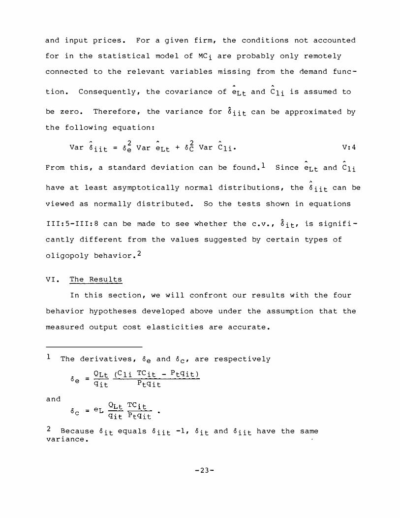
and input prices. For a given firm, the conditions not accounted
for in the statistical model of MCi are probably only remotely
connected to the relevant variables missing from the demand func
tion. Consequently, the covariance of and is assumed toeLt eli
be zero. Therefore, the variance for S iit can be approximated by
the following equation:
Var Oiit = 2
oe Var A
eLt 2
+ oc Var Cli• V: 4
From this, a standard deviation can be found.l Since eLt and eli
have at least asymptotically normal distributions, the can beOiit
viewed as normally distributed. So the tests shown in equations
I I I: 5 - I I I: 8 can be made to see whether the c.v., S itr is signi fi
cantly di f f erent from the values suggested by certain types of
oligopoly behavior.2
V I. The Results
In this section, we will con front our results with the four
behavior hypotheses developed above under the assumption that the
measured output cost elasticities ar e accurate.
The derivatives, and oc, are respectivelyoe
oe = qit Ptqit
0Lt (Cli TCit - Ptqit)
and
-1, and have the sameOit Oiit variance.
- 2 3
2

Table II gives the average c.v. 's for all the year of the
sample, al ong with the average standard deviations.! Given our
f ormulations for the c. v. 's and their variances (equations V: lb and
V: 4), tests for the hypothesi zed behavior patterns can be made for
each year. For the competitive, Cournot, and Patinkin theories, we
use a t-test for the hypothesis that the conjectural variation for
each year was signi f icantly di f f erent from the value implied by the
given type of behavior. 2 While a signi ficant di f f erence implies a
high probability of the hypothesis not being true, insigni ficant
results mean only that the c. v. value was consistent with the given
behavioral hypothesis.
To test for matching behavior we employ a t-test to see if
the c.v. is signif icantly greater than zero. Again a c. v. in the
acceptance range does not mean that the behavior was necessarily
occurring. Rather it means only that the c. v. value is consistent
with the hypothesis in question.
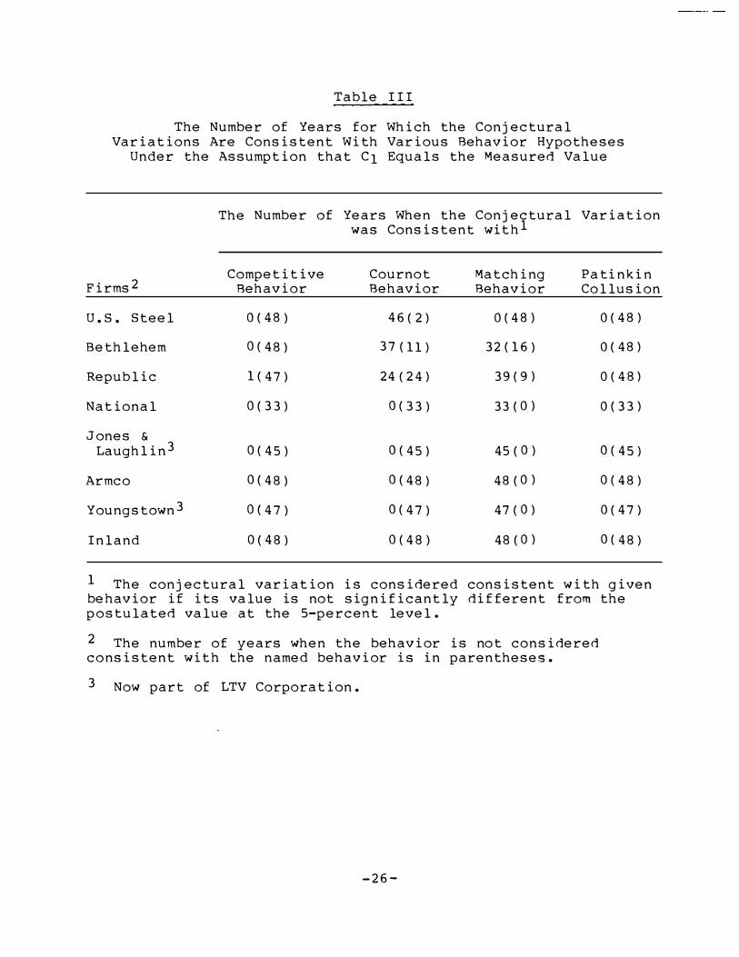
Table I I I shows the number of years in the sample for which
the c. v. values were consistent with each hypothesis. For all the
1 The average standard deviation is found by summing up the variances for the various years, dividing them by the numb er of year-observations, and calculating the square root.
2 For the competitive and Patinkin hypotheses, one-tail tests are used. These behavior patterns are extremes. A two-tail test is used for the Cournot hypothesis because it occupies an intermediate position. Matching behavior requires a one-tail test because it merely implies c. v. 's of greater value than zero. In this sample there are observations where the one-tail tests for matching behavior and the two-tail tests for the Cournot theory are inconsistent.
- 24

-3 . 96*
Table II
The Average Conjectural Variations for the ''Big Eight" Steel Comp anies for 1920-40 and 1946-7 2, and t-Test Values for
the Hypotheses that the Calculated Values Differed from the Expected Values for Comp etitive, Cournot, and Patinkin Behavior
Under the Assumption that C1 Equals the Measured Value
t-Values for
Average Conjectural Standard Corrpetitive Cournot Patinkin
Firm Variation Deviation Behavior Behavior Collusion
u.s. Steel 0. 016 0. 288 3. 53 * 0. 06 -4 .80 *
Bethlehem 1. 371 0. 767 3. 09* 1. 79* -4 .41 *
Republic 2. 979 1. 668 2. 39* 1. 79* -6. 22 *
National 5. 221 2. 061 3.02* 2. 53 *+ -4 .08 *
Jones & laughlin! 5. 869 1. 917 3. 58* 3. 06 *+
Arm:::o 10 .499 4.426 2. 59* 2. 37* + -3 .13 *
Yrungstownl 5. 657 1. 899 3. 51 * 2. 98* + -6 .03 *
Inland 4. 617 1. 755 3. 20 * 2. 63 *+ -7. 81 *
+ Significant at the 95 -percent level on a two -tail test.
* Significant at the 95 -percent level on a one -tail test.
1 No.v part of the LTV Corporation .
-25
0( 48)
1( 47)
0 ( 3 3)
0( 45)
0( 48)
0( 47)
0( 48)
46( 2)
37(11)
24( 24)
0( 33)
0( 45)
0( 48)
0( 47)
0( 48)
0( 45)
0( 48)
0( 47)
0( 48)
Table I I I
The Number of Years for Which the Conjectural Variations Are Consistent With Various Behavior Hypotheses
Under the Assumption that C1 Equals the Measured Value
The Number of Years When the Conjectural Variation was Consistent wit hl
Competitive Cournot Matching Pat ink in Firms 2 Behavior Behavior Behavior Collusion
u.s. Steel 0(48 ) 0(48) 0(48)
32(16) 0( 48)
39(9) 0(48)
Bethlehem
Republic
National 33(0) 0(33)
Jones & Laughlin3 45(0)
48(0)Armco
Youngstown3 47(0)
48(0)Inland
1 The conjectural variation is considered consistent with given be havior if its value is not significantly dif ferent from the postulated value at the 5-percent level .
2 The number of years when the behavior is not considered consistent wit h the named behavior is in parentheses.
3 Now part of LTV Corporation.
- 26

firms, the hypothesis of perf ectly competitive behavior can be
rejected for the great bulk of the sample. In no year could the
hypothesis be accepted for u.s. Steel, Bethlehem, National,
Jones & Laughlin, Armco, Youngstown and Inland. For Republic, the
hypothesis cannot be rejected in only one year, 19 21 --a depressed
year. Conspicuous about these results is that for the given firms
they hold over most of the sample.
On the other hand, when the Cournot hypothesis is examined,
the results for some firms do not show such a consistency across
time. For u.s. Steel, however, the bulk of the yearly c.v. 's are
not signi ficantly di f f erent from zero implying that Cournot
be havior cannot be rejected. Bethlehem and Republic seem to be
the intermediate cases. For Bethlehem, the Cournot hypothesis is
suppor ted in 37 of the 48 years, and for Republic there is
evidence in favor of the Cournot hy pothesis for half of the sample
( 2 4 years). In the case of Bethlehem, the Cournot hypothesis can
only be rejected for some years in the 19 20 's and 30 's. On the
other hand, it was not only for the 19 20 's but also for most of
the 1950 's and 1960 's that the Republic c.v. 's were signi f icantly
dif ferent from zero on a tw o-tail test. For the remainder of the
firms, the Cournot hypothesis can be rejected for the whole of the
sample.
Since the test for the matching behavior implies c.v. 's
greater than zero, one uses a one-tail test instead of the two
tail test. Except for u.s. Steel, generally the firm c.v. 's ar e
- 2 7

greater than zero. For Bethlehem, the one -tail test of ten contra
dicts the two -tail test; zero c.v. 's can be rejected in favor of
matching behavior for 3 2 years. For 21 of those years, however,
Cournot behavior cannot be rejected on a tw o-tail test. For
Republic using a one -tail test led to the rejection of Cournot in
favor of matching behavior in 39 years of the sample. Conse
quently some skepticism must be exercised in attributing matching
behavior to these firms for some years. Generally these consisted
of the 19 20 's and the years between 1948 and 1969. For National,
Jones & Laughlin, Armco, Youngstown, and Inland, the one - and
two-tail tests were generally consistent with matching behavior
f or the entirety of the period. The Patinkin collusion hypothesis
can be rejected for all of the sample for all the firms.
By taking an average of the c.v. 's for each firm over the
sample, we can get a summary view of the results. Table II shows
the mean and average standard deviation of the yearly c.v. 's for
each firm. All are greater than zero, the largest being that of
Armco. Consistent with the yearly results, the average c.v. 's ar e
signi f icantly di f f erent from -1, competitive behavior, for all
firms. The results on the averages show that for five firms,
Cournot behavior can be rejected on a two-tail test. As stated
above, for matching behavior a positive one-tail test for the zero
c.v. is used. For the average c.v., the results ar e consistent
with matching behavior for all firms except u.s. Steel. As wit h
the yearly results, the Patinkin hypothesis can be rejected for
all the firms.
-28
Sensitivity Analysis
To summarize, in most years, Cournot behavior cannot be
rejected for u.s. Steel and Bethlehem. The matching hypothesis is
generally consistent with the results for the other six firms, and
for no firms are the measurements generally consistent with the
competitive or Patinkin theories. With the yearly results, the
c.v. 's generally fall into the same acceptance or rejection
intervals for the great bulk of the sample for all firms except
Bethlehem and Republic with the Cournot theory.
V I I.
Because of measurement problems in the cost equations, a
sensitivity analysis will be undertaken for variations in the
cost -output elasticities.! The major sources for these variations
are first the stochastic nature of the cost estimation procedure
(multiple regression) and second possible errors in the total cost
variable used. It is not clear that the accounting measure we
used to represent short -run cost is appropriate.
The cost figure used is sales minus op erating income (before
taxes and before interest on debt) minus depreciation. This
differs from the normally presented concept of cost, sales minus
operating income, in that depreciation expense has been taken
Alternative models of demand result in elasticities (from about -0.69 to -0.75) not significantly different from the one used here. (See Rogers 1983c). So we will not test for varying demand elasticities.
-29
1
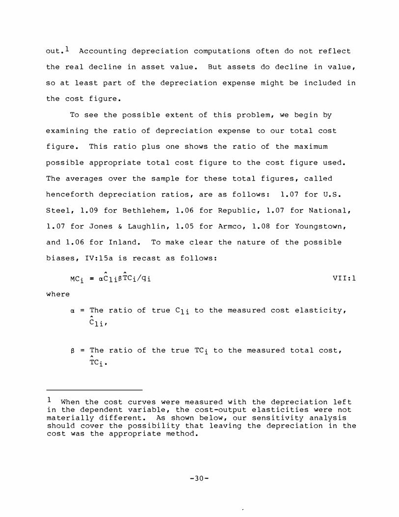
out.l Accounting depreciation computations often do not reflect
the real decline in asset value. But assets do decline in value,
so at least part of the depreciation expense might be included in
the cost figure.
To see the possible extent of this problem, we begin by
examining the ratio of depreciation expense to our total cost
figure. This ratio plus one shows the ratio of the maximum
possible appropriate total cost figure to the cost figure used.
The averages over the sample for these total figures, called
henceforth depreciation ratios, are as follows: 1.07 for u.s.
Steel, 1.09 for Bethlehem, 1.06 for Republic, 1.07 for National,
1.07 for Jones & Laughlin, 1.05 for Armco, 1.08 for Youngstown,
and 1.06 for Inland. To make clear the nature of the possible
biases, IV: l 5a is recast as follows:
A A
Mei = aCliSTCi/qi V I I: l
where
a = The ratio of true to the measu red cost elasticity, eli
eli'
8 = The ratio of the true TCi to the measured total cost,
TCi•
When the cost curves were measured with the depreciation lef t in the dependent variable, the cost-output elasticities were not materially different. As shown below, our sensitivity analysis should cover the possibility that leaving the depreciation in the cost was the appropriate method.
-30
1

The above depreciation ratios are the maximum plausible values for
e. They give an indication of how much accounting measurement
problems could bias the estimate. The formula also suggests aoi
way to correct for this problem. To illustr ate, use u.s. Steel as
an example, and assume a equals one (with eli equalling 0.695).
A
The depreciation ratio, 1.07, is the maximum e. Then, if eTCi
were the true total cost and if C! i were represented to be
which equals 0.744, then, an accurate measurement of the c.v.
would be made. It is not possible to know the real e, but the
above ratios give an indication of its range. Consequently,
varying the value of may not on ly be a way to see how theeli
results change for di f ferent cost elasticities but also a te st of
the sensitivity of the c.v. value to measurement error in TCi•
Therefore, to see how measurement errors could af fect the
results, the conjectural variations were estimated for three
alternatives eli 's. The largest cost elasticity we hypothesized,
1.2, assumes that the steel firms were operating in a region of
increasing costs under almost any conceivable accounting cost
measurement error. Many of the c. v. 's are less than -1, some
signi ficantly so statistically.! Such a c.v. implies that the
firm is oper ating at a point where price is less than marginal
cost. These results not only occurred during the depression when
such events might be expect8d but also in the 19 20 's and 1960 's
With the alternative simulations, it will be assumed that the has the variance measured by our cost model.eli
-31
ecli
1

when the steel industry was quite prosperous. Therefore, since
these results seem implausible, this particular simulation will be
ignored.
Two ot her alternative eli's seem more plausible; the first
is
eli = measured eli + 2 * SD(eli), the measured standard
deviation.
For the second, the output-cost elasticity equals one. The
simulation under the latter assumption not only shows what the
c.v. 's might be under constant returns but also gives an indica
tion of what they might be if ther e were slightly increasing cost
curves.
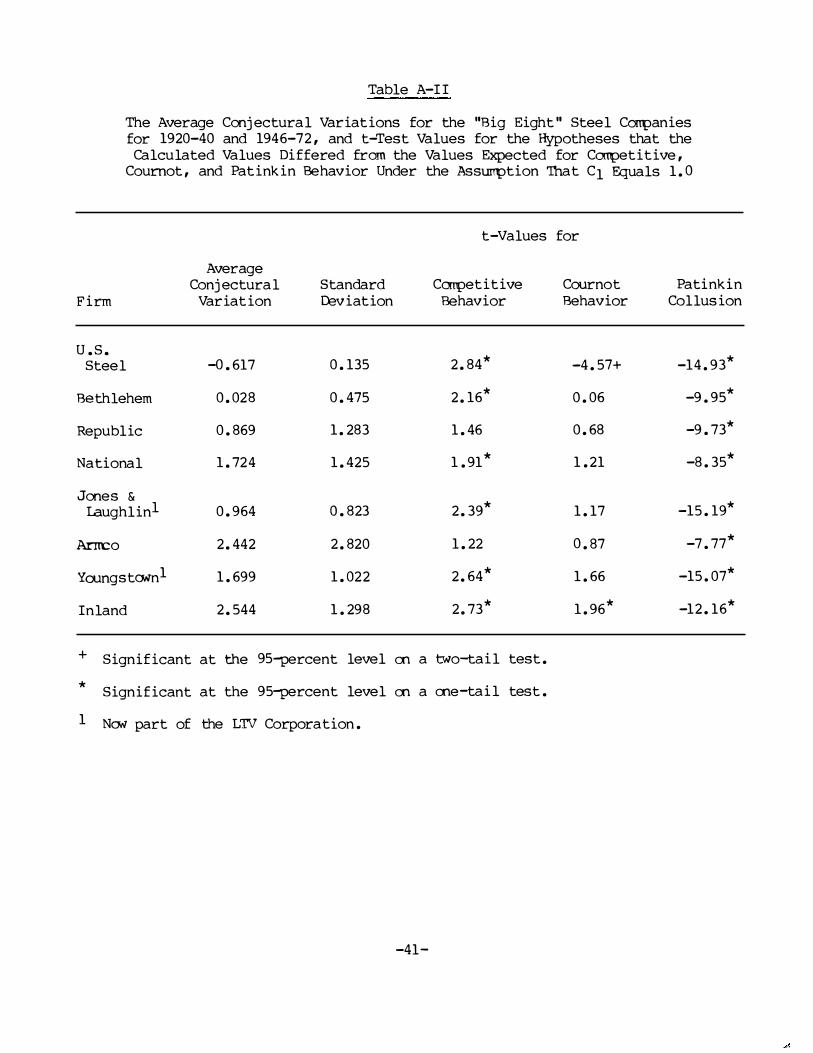
When the tests were made with the different eli's predictably
the results were mixed, but certain conclusions could be made.
(For a synopsis see the tables in the Ap pendix.) First, with the
two variations, at no time could the Patinkin hypothesis be
accepted. Second usually the competitive hypothesis could be
rejected. For the average c.v., the t test led to the rejection
of the competitive hypothesis for all firms in both variations
except for Republic under the unity assumption.eli
For the matching and eournot hypotheses, on the other hand,
the results were sensitive to changes in eli• For u.s. Steel,
assuming equal to one implies that the average c.v. waseli
significantly below zero. With the yearly results the eournot
hy pothesis could be accepted for only six years.
-3 2

With Bethlehem and Republic, the results from the two varia
tions mean that matching behavior could be rejected for the
average c.v. and the bulk of the yearly observations. On the
other hand, the acceptance of matching behavior for the smaller
firms was insensitive to the variation of Cli by two standard
deviations. But assuming a unity eli led to the rejection of the
matching hypothesis for the average c.v. for National, Jones &
Laughlin, Armco, and Youngstown but not for Inland. For these
five firms and Republic, the yearly results were generally mixed
for the matching hypothesis. Consequently for this hypothesis
the results can be sensitive to changes in the nature of the cost
structure estimates.
To sum up, pure competition and perfect collusion coulo be
rejected for all firms in most year s under all three plausible
cost structure estimates. For u.s. Steel matching behavior can be
rejected for all years under all cost assumptions. With the other
firms, however, matching behavior may sometimes not be rejected
for the two alternative eli assumptions. If the "Big Eig ht" firm
cost curves were flat or slightly upsloping, then, these firms
operated in a conjectural variation range near the Cournot or zero
point. Nevertheless, if one believes the downsloping curves as
measured by this and other papers by the author, then, matching
behavior may be accepted for the smaller five firms if not always
for Bethlehem and Republic. On the other hand, u.s. Steel seems
to have operated in a range that was close to Cournot and perhaps
even adaptive.
-33-
V I I I. Conclusion
The tests for competitive, Cournot, matching, and Patinkin
behavior show that different firms appar ently behaved differently.
Except per haps for Bethlehem and Republic, most firm c.v. 's were
fairly consistent over time. These two firms generally alternated
between c.v. 's consistent with the Cournot theory and those con
sistent with matching behavior. With the measured simulaeli
tions, the c.v. 's of Jones & Laughlin, Armco, Youngstown, and
Inland were almost always consistent with the matching hypothesis,
but for the unity simulation such behavior can only beeli
generally accepted for Inland.
The fact that the largest firm acted like a Cournot player,
while smaller firms acted in a matching fashion, seems strange.
Possibly fear of the antitrust authorities may have constrained
u.s. Steel but not the others. Also it may be that u.s. Steel was
acting in a manner that cannot be clarified from merely studying
its c.v. 's, and pe rhaps some hypotheses on interfirm relationships
should be examined. Furthermore, the cost str ucture of u.s. Steel
may have prevented more restrictive behavior. At low capacity
utili zation rates, a hig h cost firm can not hold back output as
much as other companies. There is some evidence that this firm
was not particularly efficient and mig ht even have been a high
cost pr oducer (see Weiss, 1971). The specific inter -firm
relationships that led this situation may be the subject for
another paper.
-34

To summari ze, with our methodology it was found that during
the sample period the major American steel firms conformed to two
basic behavior patterns: one was close to Cournot but signifi
cantly different from competitive. It was followed by u.s. Steel
and at least sometimes by Bethlehem and Republic. A second
pattern generally followed by the other five "Big Eight11 firms,
was usually consistent with matching behavior. These results were
not particularly sensitive to small variations in the estimated
cost parameters. But they did change somewhat when the average
cost curves were assumed to be flat.
Consequently, this methodology can be used to study and
analyze the position of various olig opoly firms on the continuum
between competitive behavior and Patinkin collusion. Neverthe
less, while one may be able to place a firm at a point in this
range, the methodology can not shed light on how it got there.
Still this analysis can show how well or poorly given firms and
industries per form; thereby perhaps indicating where antitrust
re sources should be focused.
-35
Report.
Directory
Brookings Papers
Theory
Industry.
Competitiveness,
REFERENCES
American Iron and Steel Institute. Washington D.C.: American Iron
Annual Statistical and Steel Institute,
1910-1975 various issues.
of Iron and Steel Works for the United States and Canada. Washington, D.C.: American Iron and Steel Institute, 1964, 1967, 1970 and 1974.
American Metals Market. Metal Statistics 1974. New York: American Metals Market Fairchild Publications, Inc., 1974.
Anderson, F. J. "Market Performance and Conjectural Variation." Southern Economic Journal 44, no. 81 (July 1977): 173-78.
Anderson, J. E., and Kraus, M. "An Econometric Model of Airline Flight Scheduling Rivalry." Boston: 1978 (Manuscript).
Bosworth, B. "Capacity Creation in Basic-Materials Industries." on Economic Activities 2 (1 976).
Cournot, A. Researches into the Mathematical Principles of the of Wealth. Translated by N. T. Bacon, 2d ed. New
York: Kelley, 1971.
Daug herty, C. R.; De Cha zeau, M. G. and Stratton, s. s. Economics of the Iron and Steel New York: McGraw-Hill, 1937.
Diewert, w. E. "Applications of Duality Theory." Frontiers of Quantitative Economics by M. D. Intriligator and D. A. Kendrick. Amsterdam, Oxford: North Holland Publishing Co., 1974, pp. 105-71.
Duke, R., Johnson, R., Mueller, H., Qualls, D., Roush, c. and Tarr, D. The United States Steel Industry and Its International Rivals: Trends Factors, Determining International (Bureau of Economics, Federal Trade Commission, Washington, D.C.: USGPO, 1977).
-36
Theory: Approach.
Age,
Paper Managerial Kellogg Management
University,
Productivity
Productivity
REFERENC ES (Continued)
Fama, E. F. and Laffer, A. B. "The Number of Fir ms and Competition." American Economic Review 62 (September 197 2 ): 670-74.
Gollop, F. M. and Roberts, M. J. "Firms Inter dependence in Oligopolistic Markets." Journal of Econometrics 10 (1979): 313-31.
Hekman, J.S. "An Analysis of the Changing Location of Iron and Steel Production in the Twentieth Century, " Ph.D. dissertation, University of Chicago, 1976.
"An Analysis Production in the Review 68, no. 1
Henderson, J. M. and Quandt, Mathematical
R. E. Microeconomic A New York: McGraw-Hill, 1958.
of the Changing Location of Iron and Steel Twentieth Century." American Economic
(March 1978): 1 2 5-133.
Hicks, J. R. "Annual Survey of Economic Theory: The Theory of Monopoly." Econometrica 3 (January 1935): 1- 20.
Iron vols. 175- 213 , 1955-73.
Iwata, G. "Measurement of Conjectural Variations in Oligopoly." Econometrica 42, no. 5 (September, 1974): 947-66.
Kamien, M. I. and Schwartz, N. L. "Conjectural Variations." Discussion No 46 6S Economics and Decision Service, J.L. Graduate School of Northwestern 1981.
Kendrick, J. W. Postwar in the United States. New York: National Bureau of Economic Research, 1973.
Trends in the United States. Princeton: Princeton University Press, 1961.
-37

Quarterly
Working Paper
Policy,
REFERENCES (Continued)
Klein, L. A Textbook of Econometrics. Evanston, IL: Row Peterson, 1953.
Kmenta, J. Elements of Econometrics. New York: Macmillan Company 1971.
Mancke, R. "New Determinants of Steel Prices in the u.s.: 1947-65." Journal of Industrial Economics 16 no. 2 (April 1968):147-60.
Moody's Investors Service. Moody's Industrial Manual. New York: Moody's Investors Service, 1910-1975.
Parsons, D.O. and Ray, E. J. "The United States Steel Consolidation: The Creation of Market Control." Journal of Law and Economics 18, no. 1 (April 1975):180- 219.
Patinkin, D. "Multi-Plant Firms, Cartels, and Imperfect Competition." Journal of Economics 61 (February 1947):173- 205.
Rippe, R. D. "Wages Prices and Imports in the American Steel Industry." Review of Economics and Statistics 5 2 (February 1970):34-46.
Rogers, R. P. "The Behavior of Firms in an Oligopoly Industry: A Study of Conjectural Variations." Ph.D. dissertation, The George Washington University, 1983a.
"The Measurement of Firm Cost Curves in the Steel Industry." Federal Trade Commission, Bureau of Economics
No. 96, September 1983.
"Unob servab le Transactions Price and the Measurement of a Supply and Demand Model for the American Steel Industry." Washington, D.C.: 1983c (Manuscript).
Rowley, C. K. London: McGraw-Hill 1971.Steel and Public
-38
Survey Supplement,
Analysis.
1971.
-39-
John Wiley & Sons,
REFERENCES (Continued)
u.s. Department of Commerce, Bureau of Census. Census of Manufactures 191-197 2. 1919-75.
u.s. Department of Commerce, Bureau of the Census, Statistical Abstract of the United States: 1980 (lOlth edition) 1980.
u.s. Department of Commerce, Bureau of Economic Analysis. of Current Business, 1975 1976.
u.s. Department of the Interior, Bureau of Mines. Minerals Yearbook: Fuels. 1960, 1964, 1966, 1 70, and 1973.
Varian, H. R. Microeconomic New York: w. w. Norton, 1978.
Weiss, L.W. Case Studies in Americ an Industry. New York:

Table A-I
The Average Conjectural Variations for the "Big Eight" Steel Conp anies for 19 20-40 and 1946-72, and t-Test Values for the Hypotheses that the Calculated Values Differed fr om the Expected Values for Competitive, Coornot, and Patinkin Behavior Under the AsSunt>tion that C1 equals the
Measured Value Plus TWo Times the Standard Deviation
t-V alues for
Average Conjectur al Standard Caq;>etitive Cournot Pat ink in
Firm Variation Deviation Behavior Behavior Collusion
u.s. Steel -o.134 0.250 3.46 * -0.54 -6.13 *
Bethlehem 0.68 2 0.605 2.78 * 1.13 -6. 73 *
Republic 1.419 1. 359 1.78 * 1.04 -8.78 *
National 2.812 1.59 2 2.39 * 1. 77 * -6.79 *
Jones & Iaughlinl 4.674 1.62 2 3.50 * 2.88 * -5.4 2 *
.Arrrco 6.787 3.504 2.22 * 1. 94 * -5.01 *
Yoongst&nl 4.330 1.579 3.38 * 2.74 * + -8.09 *
Inland 2.985 1.387 2.87 * 2.15 * + -11.06 *
+ Significant at the 95-percent level on a two-tail test.
* Significant at the 95-percent level 00 a me-tail test.
1 N& part of the LTV Corpor ation.
-40
-4.57 +
Table A-II
The Average Conjectural Variations for the "Big Eight" Steel Carrp anies for 19 20-40 and 1946-7 2, and t-Test Values for the Hypotheses that the
Calculated Values Differed fr om the Values Expected for Competitive, Cournot, and Patinkin Behavior Under the Assump tion That C1 Equals 1.0
t-V alues for
Aver age Conjectur al Standard Crnpetitive Cournot Pat ink in
Firm Variation viation Behavior Behavior Collusion
u.s. Steel -o.617 0.135 2.84 * -14.93 *
Bethlehem 0.0 28 0.475 2.16 * 0.06 -9.95 *
Republic 0.869 1. 283 1.46 0.68 -9.73 *
National 1.724 1.4 25 1. 91 * 1.21 -8.35 *
Jones & I.aughlinl 0.964 0.8 23 2.39 * 1.17 -15.19 *
Arm:::o 2.44 2 2.8 20 1. 22 0.87 -7.77 *
Ya.mgs tONn 1 1.699 1.02 2 2.64 * 1.66 -15.07 *
Inland 2.544 1. 298 2.73 * 1.96 * -1 2.16 *
+ Significant at the 95-percent level en a two-tail test.
* Significant at the 95-percent level en a ene-tail test.
1 No.Y part of the LTV Corporat ion.
-41

0 ( 48)
0 ( 48)
5 ( 43)
0 ( 33)
0 ( 45)
1 ( 47)
0 ( 47)
0 ( 48)
45 ( 3)
41 ( 7)
27 ( 6)
0 ( 45)
7 ( 41)
0 ( 47)
9 ( 3 9)
5 ( 43)
8 ( 40)
45 ( 0)
47 ( 1)
47 ( 0)
41 ( 7)
o ( 4 8')
0 ( 48)
0 ( 48)
0 ( 33)
0 ( 45)
0 ( 48)
0 ( 47)
0 ( 48)
Table A- I I I
The Number of Years for Whic h the Conjectural Variations ar e Consistent with Various Behavior Hypotheses Under the
Assumption that equals the easured Plus Tw o TimesC1 C1 the easured Standard Deviation
The Number of Years When the Conjectural Variation was Consistent withl
Competitive Cournot Matching Pat ink in Firms2 Behavior Behavior Behavior Collusion
36 ( 1 2) 0 ( 48)U.s. Stee 1
Bethlehem
Republic
National
Jones & Laughlin3
Armco
Youngstown3
Inland
21 ( 1 2 )
1 The conjectural variation is considered consistent with given behavior if its value is not significantly dif ferent from the postulated value at the 5-percent level.
2 The number of years when the behavior is not considered consistent with the named behavior is in parentheses.
3 Now part of LTV Corporation.
-4 2

4(44)
7( 26)
2(46)
6( 4 2)
48(0)
33(0)
0( 48)
0( 48)
0(48)
0( 33)
Table A- IV
The Number of Years for Which the Conjectural Variations are Consistent with Various Behavior Hypothese s
Assuming Equals 1.C1
The Number of Years When the Conjectural Variation was Consistent withl
Competitive Cournot Matching Pat ink in Firms 2 Behavior Behavior Behavior Collusion
0 ( 48)u .s. Steel 2(46)
Bethlehem 0(48)
Republic 10(37)4 41(7) 6(4 2 )
National
Jones &
3 ( 30)
Laughlin3 6( 39) 40(5) 15(30) 0(45)
Armco 14(34) 44(4) 14(34) 0(48)
Youngstown3 3 ( 44) 29(18) 35(1 2) 0(47)
Inland 28( 2 0) 41(7) 0(48)
1 The conjectural variation is considered consistent with given behavior if its va lue is not significantly different from the postulated value at the 5-percent level.
2 The number of years when the be havior is not considered consistent with the named behavior is in parenthe ses.
3 Now part of LTV Corporation.
4 One observation was significantly less than -1.
-4 3