the matlab tm software application for electrical

Chapter 18

© 2012 Lessa et al., licensee InTech. This is an open access chapter distributed under the terms of the Creative Commons Attribution License (http://creativecommons.org/licenses/by/3.0), which permits unrestricted use, distribution, and reproduction in any medium, provided the original work is properly cited.

The MatLabTM Software Application for Electrical Engineering Simulations and Power System

Leonardo da S. Lessa, Afonso J. Prado, Rodrigo Cleber Silva, Sérgio Kurokawa, Luiz F. Bovolato and José Pissolato Filho

Additional information is available at the end of the chapter

http://dx.doi.org/10.5772/48555

1. Introduction

Transmission lines are the elements of the electric power system that connect the load to the generation joining the production facilities of energy over large geographic areas. You could say that the transmission of electricity is one of the most important contributions that engineering has offered to the modern civilization.

The distribution of current potential differences and the transfer of energy along a transmission line can be analyzed by various methods, and it is expected that all lead to the same result. In engineering problems, in general, it can not indiscriminately apply a single formula for solving a specific problem, without the full knowledge of the limitations and simplifications accepted in its derivation. It is worth mentioning that this circumstance would lead to its misuse. The so-called mathematical solutions of physical phenomena typically require simplifications and idealizations.

Therefore, there are several models that represent the transmission lines and can be classified as to the nature of their parameters in the model parameters constant and variable parameters the models with frequency.

The parameters in the models in terms of frequency are easy to use, but can not adequately represent the line in the entire range of frequencies at which these phenomena are transient in nature. In most cases, these designs increase the amplitude of the high order harmonics, distorting the waveform peaks and producing exaggerated errors.

For adequate representation of the transmission line should be considered that the longitudinal line parameters are strongly frequency dependent, including the variable

MATLAB – A Fundamental Tool for Scientific Computing and Engineering Applications – Volume 3 434

parameters in the models with frequency, the sum of the effect of soil, developed by Carson and Pollaczek, with skin effect, whose behavior as a function of frequency can be calculated using formulas derived from the Bessel equations.

Models with variable parameters in terms of frequency are considered more accurate when compared to models that consider the constant parameters. The variation depends upon the frequency. This variation may be represented by series and parallel combination of resistive and inductive elements pure.

As transmission lines are inserted in an electrical system that has many nonlinear elements and, thus, it is difficult to represent them in the frequency domain, there is a preference for line models that are developed directly in the time domain.

Another factor, that makes the model lines developed directly in the time domain are most commonly used, is that the majority of programs that perform simulations electromagnetic transients in electrical systems require that the system components are represented in time domain.

Probably, the first model to represent the transmission line directly in the time domain is designed for H. W. Dommel, which was based on the method of the characteristics or Bergeron’s method. The model has combined the method of characteristics with the trapezoidal method numerical integration, resulting in an algorithm able to simulate transient electromagnetic networks whose parameters are distributed or discrete. This algorithm has undergone successive developments and is now known as the Electromagnetic Transients Program, or EMTP simply.

In situations where one wants to simulate the propagation of electromagnetic waves resulting from operations carried out maneuvers and switching the transmission lines, it can be represented the same as a cascade of π circuits.

In this model, each segment consists of a combination of series and parallel circuits composed by resistors and inductors. This results in an equivalent resistance and an inductance that depend on the frequency. It is considered in hese equivalent elements the ground and skin effects.

Due to the fact that EMTP-type programs are not easy to use, several authors suggest describing the currents and voltages in the cascade of π circuits by means of state variables. The state equations are then transformed into differential equations and can be solved using any computer language or mathematical software.

The representation of the line by means of state variables can be used in teaching basic concepts of wave propagation in transmission lines, the analysis of the distribution of currents and voltages along the line, and the simulation of electromagnetic transients in transmission lines with non-linear elements.

Although the technique of state variables is widely used in the representation of transmission lines, it can be seen in recent publications, that it was only used to represent

The MatLabTM Software Application for Electrical Engineering Simulations and Power System 435

the parameters of which longitudinal rows can be considered constant and independent of frequency.

However, it is recognized today that the use of constant parameters to represent the line in the whole frequency range, present in the signals during the occurrence of disturbances in it, may result in responses in which the high frequency harmonic components have larger amplitudes than the real ones.

Thus, in this chapter, it is intended, using the MatLabTM, to enter the effect of frequency on a line represented by π circuits connected in cascade and obtain the currents and voltages on the line from the use of the technique of state variables. The method is applied in a single-phase line, which considers the presence of soil and peel effect.

This line is approximated by a cascade of π circuits which will then be represented by state equations. The state equations, which are the voltages and currents along the line, will then be simulated in MatLabTM. The cascade will also be implemented in software such as EMTP, used for simulations of electromagnetic transients in power systems. Then the results obtained with MatlabTM and EMTP are compared, considering the single-phase line.

Besides this mentioned modeling, for MatLabTM software users, the main contribution of this chapter is to demonstrate the application of this program for analyzing and simulating transient phenomena in power systems. It is important for undergraduate students for understanding the basic concepts of wave propagation and transmission lines. On the other hand, specific programs, like EMTP type programs, use a specific numeric method for solving the linear systems through numeric integration. With MatLabTM basic tools, the graduate students can apply different numeric methods for solving the same problem, comparing the results and analyzing the accuracy, precision and computational time related to each method.

2. Trapezoidal integration

It is a brief equation that relates the numerical method for lumped parameters used by the ATP. Is an arbitrary differential equation given by:

( )( ) dx ty t kdt

(1)

The solution between the instants t0 and t is obtained by the following:

0 0 0

01 1 1( ) ( ) ( ) ( ) ( ) ( )

x t t

x t t

dx t y t dt x t dx y t dt x t x y t dtk k k

(2)

or finally:

0

01( ) ( )

t

tx t x y t dt

k (3)


The numerical solution of the equation is obtained at discrete instants of time, given:

( )

( )

1 1 1( ) ( ) ( ) ( ) ( )x t t t

x t t t t t txdx dx t y t dt x t x t t y t dt

k k k (4)

The solution of equation (2.4) consists of numerical integration of a discrete function y(t) which must be performed in discrete steps size Δt, which solution is the area under the curve, limited by the instants t and t-Δt as shown in Figure 1.

(a) (b)

Figure 1. (a) function y(t) slight to be integrated; (b) trapezoidal rule integration.

Solving equation (2.5) by the trapezoidal rule integration, which allows a linear variation between y (t-Δt) and y (t) of the integrated, as shown in figure 1 (b), as:

( ) ( )1 1( ) ( ) ( ) ( )2

t

t t

y t y t tx t x t t y t dt x t t tk k

(5)

or:

( ) ( ) ( ) ( )2 2

t tx t y t x t t y t tk k

(6)

in other words:

( ) ( )TR TRx t C y t h t t (7)

where:

2

( ) ( ) ( )2

TR

TR

tCk

th t t x t t y t tk

(8)


It may be noted that the term historical hTR(t-Δ t) depends on x (t) and y (t) after t seconds, t, is already known during the solution.

3. Modeling cascada of π circuits

Discussion will now represent a mathematical model for a transmission line using an electrical circuit. With this model, you can make a study of the behavior of a transmission line for energizing and switching transient simulations. A transmission line, whose parameters can be considered independent of frequency, can be represented in an approximate manner and following a series of restrictions, as a cascade of π circuits.

Each segment of π circuit consists of one resistor and one series inductance in series. Completing the circuit, there are components in parallel: capacitance and conductance. It is shown in Figure 2.

Figure 2. A π circuit.

It’s represented a transmission line through this model, connects to n π circuits in cascade. So Figure 3 shows a single-phase transmission line length d represented by n π circuits connected in cascade.

Figure 3. Line represented by a cascade of π circuits.

In Figure 3, the parameters R and L are the resistance and inductance of the longitudinal line, respectively. The parameters G and C are the capacitance and conductance of transverse dispersion, respectively. These parameters are written as:

' dR Rn

(9)

' dL Ln

(10)

G2

C2

G2

C2

R L


' dG Gn

(11)

' dC Cn

(12)

In the equations (3.1) to (3.4), R 'and L' are the resistance and inductance of the longitudinal row per unit length, respectively while the terms G 'and C' are the capacitance and conductance per unit cross-sectional line in length.

Using this representation of the line, a state model is formulated for the energy system that uses the voltages on the capacitors and the currents through the inductors as state variables. The system that describes the state equations is transformed into a set of differential equations whose solution is given by the use of trapezoidal integration. The state variables are found by solving the set of equations.

Although the technique of state variables is widely used in the representation of transmission lines, it is applied only to depictions of longitudinal lines whose parameters can be considered constant and independent of frequency.

However, it is recognized today that the use of constant parameters to represent the line in the whole frequency range, present in the signals during the occurrence of disturbances in it, may result in responses in which the high frequency harmonic components have larger amplitudes than are actually.

4. Line representation with parameters of frequency dependent

The representation of transmission lines through cascades of π circuits, taking into account the effect of frequency, is usually implemented in EMTP-type programs.

Another drawback of the type EMTP programs is that they limit the amount of π circuit that can be used to represent the line. Thus, depending on the length of the line to be depicted, the quality of results obtained from simulations may be compromised.

To circumvent the difficulties mentioned, it is suggested to describe the cascade of π circuits by means of state equations. However, some authors disregarded the effect of frequency on the parameters of the longitudinal line.

Figure 4. Circuit that represents the longitudinal parameters of the line.


The models proposed by would become more complete if the effect of frequency on the longitudinal parameters of the line was inserted in them.

So, the parameters of a transmission line can be synthesized by means of a circuit of the type shown in Figure 4.

It’s used a cascade of π circuits to represent a transmission line taking into account the effect of frequency on the longitudinal parameters. In this case, every π circuit will be shown in Figure 5.

Figure 5. Cascade of π circuits considering the effect of frequency.

In Figure 5, the RL parallel associations are as many as necessary to represent the variation of parameters in each decade of frequency that will be considered. First, arrays are displayed in a state for a line represented by a single π circuit, whereas the effect of frequency is synthesized by n RL associations. Then, the results will be extended to a line represented by a cascade of n π circuit, considering n RL associations to synthesize the effect of frequency.

Before being certain state equations for a line represented by a cascade of n π circuits, it will be shown in detail the development of equations of state considering only one π circuit.

Then, the development done for a single π circuit element can be extended to a generic cascade with any quantity of these circuits.

Considering, as shown in the Figure 5, a transmission line represented by a single π circuit, the effect of frequency on the longitudinal parameters is represented by n RL associations.

In line shown in Figure 5, the voltages at terminals A and B are u(t) and vk(t), respectively. It is also considering that the currents ik0, ik1, ..., ikm are circulating through the inductors L0, L1, L2, ..., Lm, respectively. These currents are dependent time functions and the notations do not include the time dependence for more simplicity. This simplification is also applied to the vk(t) state variable. From the currents and voltages in the circuit of Figure 5 it can be determined:

0 0

1 10 0 0 0

1 1 1( )m m

k kj j k j k

j jL

di iR R i u t v

dt L L L L

(13)


1 1 10 1

1 1

kk k

di R Ri i

dt L L (14)

2 2 20 2

2 2

kk k

di R Ri i

dt L L (15)

0k m m m

k k mm m

di R Ri i

dt L L (16)

0( ) 2 ( )k

k kdv t Gi v t

dt C C (17)

The equations (4.1) to (4.5), describing the circuit shown in figure 4.2, can be written as:

x Ax Bu (18)

For one circuit, the A matrix is substituted by:

0 1 2

0 0 0 0 0

1 1

0 0

2 2

2 2

1

0 0 0

0 0 0

0 0

0 0 0

2 0 0 0

j m

jj m

m m

m m

RRR R

L L L L L

R RL L

R RL L

A

R RL L

GC C

(19)

0

1 0 0 0 0TBL

(20)


0 1 2Tk k k k k m kx i i i i v (21)

1 20T

k k k mk k kk

di di didx di dvx

dt dt dt dt dt dt

(22)

In the equations (4.8) and (4.9), BT e xkT correspond to transposed B and xk, respectively.

The obtained results show that the vesctor xk have (m + 2) elements and the matrix A is a (m + 2) order square matrix.

Based on the equations and the results for one π circuit, it can be extended the analysis to a cascade of π circuits. Thus, the matrix A will have an order of n(m +2) and the vector x has dimension n(m +2). The A matrix can be written as:

11 12

21 22 23

32 33

43 3 2

2 2 2 1

1 2 1 1 1

1

0 0 0 00

0 0 00 0 0 0

0 0 0

0

0 0 0 0

n n

n n n n

n n n n n n

nnn n

A AA A A

A AA A

AA A

A A A

A A

(23)

The elements x1, x2, …, xn are describe by equation (4.9). In equation (4.11), A is a tridiagonal matrix which elements are square matrices of order (m +2). In this case, a generic element AKK at main diagonal of the matrix A is written as:

kkA A (24)

The A π matrix is defined in equation (4.7).

An element of any upper subdiagonal in equation (4.11) is a square matrix of order (m +2) which the only one nonzero element is located in the first column of last row and has the

value 1C

.

The structure is:

0 0 0

01 0 0

1, 2

ikA

Ci k k n

(25)


The subdiagonal elements in the equation (4.11) are square matrices of order (m +2). These arrays have a single nonzero element which is in the last column of first row. It is a value of

01

L

. The structure is:

010 0

0

0 0 01, 1 1

ik

L

A

i k k n

(26)

Considering a cascade of π circuits, the vector B has the dimension of n(m +2) and if it is connected a u(t) source at the beginning of the line, the vector B has a single nonzero

element, which is the first array element and it has the value 0

1L

.

The state equation, that describes a line representation by a cascade of π circuits cant be solved by numerical methods, like Euler and Heun methods. Other numeric methods are described in the next item

5. Other numeric methods

Besides the trapezoidal integration, there are also other numeric methods that can be used for solving state equations related to the modeling of transient phenomena in transmission lines. Among them, it may be mentioned, for example, the Simpson’s and the Runge-Kutta’s method. The following items will describe these methods. In this case, the MatLabTM is important because it facilitates the comparisons among the mentioned methods. With this software, undergraduate students can analyze the application of different numeric methods for solving an engineering problem, besides the analysis about wave propagation and the transmission line modeling. Graduated students can analyze what it is the best option for specific transmission line characteristics and develop the numeric method related to the simulation of transient phenomena in power systems.

5.1. Simpson’s rule

Simpson’s rule is based on the assumption that, given short intervals of time the derivative of the function to be integrated, the function (y') can be approximated by a second degree function as shown in Figure 6.

From Figure 1, it is obtained:

1 11 ' 4 ' '3k k M ky t y t y t y t t (27)


From (5.1) and (4.6), it is obtained:

1 1 2 3 4kx t a a a a (28)

Equation (5.2) is applied Simpson's rule for solving the state equation of state of the type shown in (5.1). In this case, the matrices a1, a2, a3 and a4 are written as:

1 6ta I A

(29)

2 6 kta I A x t

(30)

32

3 Mta A y t

(31)

4 146 k M kta B u t u t u t

(32)

It is defined the following terms:

1k kt t t (33)

1

2k k

Mt t

t (34)

Figure 6. Approximation of the derivative of the function to be integrated (solid curve) by a function of the second degree (dashed curve).

5.2. Runge-Kutta’s rule

Runge-Kutta’s rule is defined by the following:

1 1 2 3 41 2 26k kx t x t k k k k (35)


The terms in the last equation are described by:

1 k kk t A x t Bu t (36)

12 2k k

kk t A x t Bu t

(37)

23 2k k

kk t A x t Bu t

(38)

4 3k kk t A x t k Bu t (39)

5.3. Comparisons among the numeric methods

The MatlabTM software is easily applied for the development of numeric routines. Using this characteristic, it is possible to compare different numerical methods. Figure 7 shows the results for the three methods investigated for the simulation of electromagnetic transients in a single-phase transmission line.

Figure 7. Comparisons among the three numerical methods.

In the last figure, it is shown the result obtained with the application of a step voltage source on the initial transmission line. This is a 20 kV step voltage source. The transmission line is modeled as a mono-phase circuit and the linear system is solved using three numeric methods: trapezoidal rule, Simpson’s rule and Range-Kutta’s one.

Based on the results shown in Figure 7, the three numeric methods lead to similar results considering the method accuracy. Because of these results, it is necessary to analyze the other characteristics. An important characteristic for the application of the numeric methods for transient analysis in transmission lines is the simulation time. For example, this is

0 0.2 0.4 0.6 0.8 1 1.2 1.4 1.6-10

0

10

20

30

40

50

Time [ms]

Vol

t [k

V]

Heun

Simpson

Runge-Kutta


important for analysis in very short simulation times. The next table shows the simulation time comparisons obtained with the MatLabTM software.

Step of calculating (µs)

Computational effort (simulation time) Heun Simpson Runge-Kutta

0,1 t1 22,52 t1 0,63 t1 0,5 t2 8,94 t2 0,23 t2 1,0 t3 8,40 t3 0,26 t3

Table 1. Simulation time required by numerical methods

Table 1 shows the time relationship between the applied numerical methods. It is possible to carry out these comparisons because the MatlabTM provides a simple way to replace the codes related to the numeric routine without changing the structure of the main code, maintaining the same computational flowchart. Using this characteristic, it is possible to determine the simulation time of each numeric method, because the computational time for introducing the data and other characteristics of the simulated transmission line is equal for all compared numeric methods. Because of this, the MatLabTM is an adequate tool for developing new models and numeric routines used for analysis and simulations of transient phenomena in transmission lines.

6. Model implementation of single phase line

In this section, it is presented the implementation of a single-phase transmission line through a cascade of π circuits, considering the effect of frequency on their longitudinal parameters and using the concept of state variables. Then, the results obtained are compared with results obtained with EMTP.

6.1. Block diagram of the program for single-phase line

The model that represents the single-phase line was implemented in a microcomputer using the software MatLabTM.

Data from single-phase transmission line are read in the first part of the program, then the parameters are calculated from the transmission line considering the influence of frequency.

After observing the behavior of single-phase line parameters as a function of frequency, it is necessary to represent this influence on the transmission line model proposed in item 4. This was done using the method called vector fitting and the longitudinal single phase line parameters are fitted by means of rational functions.

With these parameters synthesized and distributed in the proposed model of a single-phase line, it is possible to calculate the voltages and currents at the terminals of this line or at any point of the line.


The model represented by a cascade π circuits can be represented by a linear system that is

represented by state variables. For the solution of the system represented by [ ] [ ]x A x B u ,

it’s used Heun formula (trapezoidal integration method). This method is widely used in simulations of electromagnetic transients in power systems

Figure 8 is shown a block diagram of the algorithm of the program developed for single-phase line.

Figure 8. Block diagram of the routine developed for a single-phase.

6.2. Calculation of the parameters of the transmission line single phase

It’s possible to bring the longitudinal parameters of single-phase line by means of rational functions. Using the vector fitting method and allowing the fitting the frequency dependence of these parameters, this effect is entered in the discrete parameter model.

The equation that summarizes the parameters of longitudinal single-phase line is given by:

31 2 40 0

1 2 3 4

1 2 43

( )VFITj Rj R j R j R

Z R j LR R R Rj j jjL L LL

(40)

The values of R and L in the equation (6.1) found by the method vector fitting are shown in Table 2.

From the values of Table 1, it can view a summary of the parameters of longitudinal line as follows: replacing the values of Table 1 in the expression (6.1) and attribute values are included in the frequency range 101 to 106 for it is possible to calculate the longitudinal impedance synthesized.


In the equivalent circuit, the values were considered in the frequency range from 101 to 106, because transients that occur in the transmission line are within this frequency range. So the four blocks RL in parallel, shown in Figure 9, are representing the influence of frequency on longitudinal parameters of single-phase transmission line.

Figure 9. Circuit that represents the longitudinal parameters of the line.

Resistors (Ω/km) Inductors (mH/km)

R’0 0,026 L’0 2,209 R’1 1,470 L’1 0,74 R’2 2,354 L’2 0,12 R’3 20,149 L’3 0,10 R’4 111,111 L’4 0,05

Table 2. Values of elements R e L for a single-phase.

7. Transmission line with corona effect

7.1. General aspects about the corona

The corona discharge mechanism is an electrostatic phenomenon due to ionization in an insulating material, usually a gas, subject to electric field intensities above a critical level.

Electrical discharges in gases are usually triggered by an electric field that accelerates free electrons therein. When these electrons acquire enough energy from the electric field, they can produce new electrons from the collision with other atoms. It is the process of impact ionization. During its acceleration in the electric field, each free electron collides with atoms of oxygen, nitrogen and other present gases, missing, that collision, part of its kinetic energy. Occasionally, it can achieve an electron atom with sufficient force so as to excite it. Under these conditions, the atom is achieved to a higher energy state. The orbital state of one or more electrons and the electron moves colliding with the atom loses some of its energy to create this state. Subsequently, the atom can hit revert to its initial state, releasing the excess energy as heat, light, electromagnetic radiation and acoustic energy. An electron can also collide with a positive ion, converting it into neutral atom. This process, called recombination, also releases excess energy.


7.2. Corona effect representation

After the pioneering work of Peek (1915), several measurements have made on lines and experimental laboratories have examined the nature of the corona and its influence on wave propagation in transmission lines. These works have had fundamental importance, contributing to the understanding of the basic mechanism of the corona.

In 1954, Wagner et al. (1954) and Wagner and Lloyd et al. (1955) published two articles that would be a reference for future work on corona. Voltage experimental measurements were made of in the laboratory of a conductor under corona (project called Tidd 500 kV).

Through these experimental results, it has developed empirical formulas and procedures for considering the effects of attenuation and distortion in the spread of outbreaks. These formulas and procedures are based on the voltage gradient, and voltage curves are obtained from attenuation measurements and the power dissipation due to the corona effect. The usefulness of these methods is limited however, because it requires different approaches and uses abacuses.

The corona model can be divided into three classes: analog models, mathematical models and physical models. The electrical circuit analog models are designed to reproduce the geometric increase in the capacitance of the conductor to the voltage reaches critical ionization.

Like the analog models, mathematical models roughly reproduce the characteristics of drivers under the corona, but by means of mathematical equations. Several authors have empirical formulations for the variation of capacitance of the line based on functions and constants derived from measurements. Most models show a linear relationship between capacitance and dynamic tension.

Due to the complexity in describing mathematically the physical phenomena involved and the insufficient amount of data propagation in corona, it is not available generic models of this nature yet.

7.3. Gary’s model

The equations describing the corona effect is not easily implemented in the differential equations of the transmission line in order to obtain a solution formulation easyly. Thus, to obtain responses directly in the time domain, numerical models are used such as the finite difference method and the method of the characteristics. This last category of models has been developed to be implemented in EMTP-type programs. Some of these models use non-linear resistors and capacitors that are dependent on the voltage applied on them. However, most existing models of corona present satisfactory results only for a specific situation.

The mechanism of the corona effect can also be represented by the model of Gary, using a capacitance and a non-linear conductance to represent the accumulation and the pressure drops in the line. The capacitance and conductance mentioned above are variables with the


applied voltage on them and are called corona capacitance (Cc) and corona conductance (Gc). Cc and Gc elements are obtained by known analytical function, and, therefore, this representation for the corona effect is called analytical model of the corona effect. This model for the corona effect can be inserted in lines represented by a cascade of circuits, where currents and voltages along line is described by state variables.

If the capacitance is represented by Gary’s corona model, it is defined as:

1

0

CC

C

C

vC se v VV

Cse v V

(41)

In equation (7.1), CC is the corona capacitance, C is the geometric capacitance of the line segment represented by a π circuit, v is the voltage being applied to the line capacitance, CV is the minimum voltage required to the corona effect accurrance and η is a coefficient defined as:

0,22 1,2r (42)

where: r the radius of the conductor in centimeters.

Thus, given the presence of the corona effect and the effect of frequency, a differential element row can be represented as shown in Figure 10.

Figure 10. A differential element of line considering the corona effects

The corona conductance to Gary’s model is defined as:

21 C

C CV

G kv

(43)

Gary’s model considers that the corona effect is manifested only if the voltage VC is greater than v and the rate of variation over time v is positive. Thus, if the corona effect is manifested at a given point P of the line, the voltage Vp at this point must satisfy the following conditions:


0pp C

dVV V and

dt (44)

Thus, for the corona effect is present at a generic point of the line represented by a cascade of circuits, as shown in figure 10, it is necessary that the voltage at this point satisfying the two conditions shown in equation (7.4). If a condition is not met, this point will not have increased the capacitance and conductance representing corona. Therefore, the A matrix shown in equation (4.6) should be changed for each iteration as a function of cross-line voltage.

8. Testing the model

Checking the effectiveness of the developed model, it is simulated the energizing of a transmission line shown in figure 11, considering frequency independent line parameters and frequency dependent ones.

Figure 11. Single phase line representation with opened terminal.

In Figure 11, S is a switch that be closed at time t = 0, energizing the line through a voltage source u(t). In the current procedure, the terminal B is open and the other terminal is powered by a constant voltage source. For frequency dependent line parameters, it is considered that the longitudinal parameters of the line per unit length can be perfectly summed up by a circuit consisting of four RL parallel blocks connected in series. The structure is completed using a RL series block as shown in Figure 9.

The values of R and L used to synthesize the effect of frequency on the longitudinal parameters of the line were obtained using the method proposed by [10] and are shown in Table 1. The parameters of the unit transverse line shown in figure 3 are G′=0,556 µS/km e C′ =11,11nF/km.

9. Simulation analysis of transmission lines with single phase representation

In all simulations, it is used the following values: the transmission line has 10 kilometers. It is represented through 200 π circuits. The time step used in the simulations is 50 ns and the

u(t)

Swith S


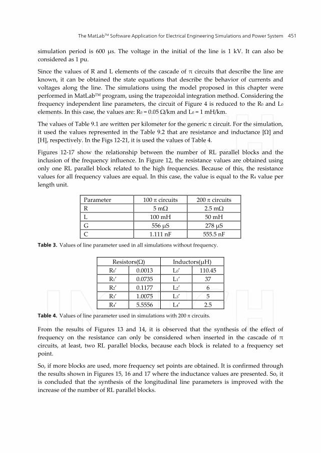
simulation period is 600 µs. The voltage in the initial of the line is 1 kV. It can also be considered as 1 pu.

Since the values of R and L elements of the cascade of π circuits that describe the line are known, it can be obtained the state equations that describe the behavior of currents and voltages along the line. The simulations using the model proposed in this chapter were performed in MatLabTM program, using the trapezoidal integration method. Considering the frequency independent line parameters, the circuit of Figure 4 is reduced to the R0 and L0 elements. In this case, the values are: R0 = 0.05 Ω/km and L0 = 1 mH/km.

The values of Table 9.1 are written per kilometer for the generic circuit. For the simulation, it used the values represented in the Table 9.2 that are resistance and inductance [] and [H], respectively. In the Figs 12-21, it is used the values of Table 4.

Figures 12-17 show the relationship between the number of RL parallel blocks and the inclusion of the frequency influence. In Figure 12, the resistance values are obtained using only one RL parallel block related to the high frequencies. Because of this, the resistance values for all frequency values are equal. In this case, the value is equal to the R4 value per length unit.

Parameter 100 circuits 200 circuits R 5 mΩ 2.5 mΩ L 100 mH 50 mH G 556 µS 278 µS C 1.111 nF 555.5 nF

Table 3. Values of line parameter used in all simulations without frequency.

Resistors(Ω) Inductors(µH) R0’ 0.0013 L0’ 110.45 R1’ 0.0735 L1’ 37 R2’ 0.1177 L2’ 6 R3’ 1.0075 L3’ 5 R4’ 5.5556 L4’ 2.5

Table 4. Values of line parameter used in simulations with 200 circuits.

From the results of Figures 13 and 14, it is observed that the synthesis of the effect of frequency on the resistance can only be considered when inserted in the cascade of π circuits, at least, two RL parallel blocks, because each block is related to a frequency set point.

So, if more blocks are used, more frequency set points are obtained. It is confirmed through the results shown in Figures 15, 16 and 17 where the inductance values are presented. So, it is concluded that the synthesis of the longitudinal line parameters is improved with the increase of the number of RL parallel blocks.


Figure 12. Synthesis of resistance per unit length using R’4L’4 parallel block.

Figure 13. Synthesis of resistance per unit length using R’1L’1 and R’4L’4 parallel blocks.

Figure 14. Synthesis of resistance per unit length using four RL parallel blocks.

101

102

103

104

105

106

110

110.5

111

111.5

112

112.5

Frequency

Ohm

/km

101

102

103

104

105

1060

20

40

60

80

100

120

Frequency

Ohm

/km

101

102

103

104

105

10620

40

60

80

100

120

140

Frequency

Ohm

/km


Figure 15. Synthesis of inductance per unit length using only R’4L’4 parallel block.

Figure 16. Synthesis of inductance per unit length using R’1L’1 and R’4L’4 parallel blocks.

Figure 17. Synthesis of inductance per unit length using four RL parallel blocks.

The result of the simulation made for the voltage input signal u(t) can be seen in Figure 18. It is shown the output voltage at the receiving end terminal of the line without the frequency

101

102

103

104

105

1060.05

0.05

0.05

0.05

0.05

0.05

0.05

Frequency

H/k

m

101

102

103

104

105

1062. 2

2.21

2.22

2.23

2.24

2.25

2.26

2.27

Frequency

H/k

m

101

102

103

104

105

1062 .2

2.25

2.3

2.35

2.4

2.45

Frequency

H/k

m


influence. Using the routine without the influence of frequency from the results of Figure. 18, it is observed that there is a period of time related to the time of signal propagation through the line.

Figure 18. Energization of the transmission line without the effect of frequency considering 200 π circuits.

Thus, it represents a time delay between input signal and output signal. After the delay, there are oscillations associated with wave reflections on the transmission line terminals that make up the output voltage shown.

Figure 19. Voltage at the end of the transmission line with the effect of frequency considering 200 π circuits.

Using the routine with frequency influence in longitudinal parameters, it is obtained the results of Figure 20. In this figure, comparing to Figure 19, the voltage signal is attenuated because the inclusion of the frequency influence.

Figures 21 and 22 show the influence of frequency on the current results. Without the frequency influence, the obtained signal current is not attenuated and is highly modified by numeric oscillations (Figure 14). On the other hand, when the routine considers the

0 1 2 3 4 5 6

x 10-4

-1

-0.5

0

0.5

1

1.5

2

2.5

3V

olta

ge [

pu]

Time [s]

0 1 2 3 4 5 6

x 10-4

0

0.5

1

1.5

2

Vol

tage

[pu

]

Time [s]


influence of frequency (Figure 22), it is clear that the current signal could not contain those oscillations shown in Figure 21. So, those oscillations are numeric oscillations and they can be associated to the representation of the longitudinal line parameters which does not consider the frequency influence.

Figure 20. Current at the end of the transmission line without the effect of frequency.

Figure 21. Current at the end of the transmission considering the effect of frequency.

So, for the sequence of this work, it should be investigated what is the saturation point for the number of the π circuits and the number of the RL parallel blocks. It is carried out using the simulation results from several voltage signals that will be used as voltage sources at the initial line terminal.

For Figures 22 and 23, using the routine without the effect of frequency, it is analyzed a particular stretch of the simulation at the end of the line. It is shown the voltage values without frequency influence. In Figures. 22 and 23 it is used the values of Table 2, using 100 and 200 π circuits, respectively.

0 1 2 3 4 5 6

x 10-4

-1

-0.5

0

0.5

1

1.5x 10

-3

Cur

rent

[A

]

Time [s]

0 1 2 3 4 5 6

x 10-4

-2

-1

0

1

2

3

4

5

6x 10

-4

Cur

rent

[A

]

Time [s]


Figure 22. Specific portion of the simulation at the end of the line with 100 π circuits and without the effect of frequency.

Based on the mentioned results, it concludes that increasing the number of π circuits leads to a decrease in the numerical oscillations.

Figure 23. Specific portion of the simulation at the end of the line with 200 π circuits and without the effect of frequency.

In Figure 23, it is clearly a greater condensation of numerical oscillations in both x and y axes in contrast to Figure 23, where the period of the oscillations and the peak value are higher than those obtained in Figure 23. In Figures 24, 25 and 26, it is used the routine with the effect of frequency, analyzing the number of the RL parallel blocks inserted in the cascade of π circuits, searching for reducing of numerical oscillations. In Figures 24, 25 and 26, it was used the values of Tables 3 and 1, as well as, 3 and 4 RL parallel blocks, respectively.

From the results of Figures 24, 25 and 19, it is observed that the used routine including the effect of frequency in the cascade of π circuits obtains considerably fewer numerical oscillations when compared to Figures 22 and 23. From these results, it is evident that if it is increased the number of the RL parallel blocks, it is reduced the numerical oscillations and the voltage in the line end has a smoothly curve in the time domain.

3 4 5 6 7 8 9 10

x 10-5

1.7

1.8

1.9

2

2.1

2.2

2.3

2.4

2.5

Vol

tage

[kV

]

Time [s]

3 4 5 6 7 8 9 10

x 10-5

1.6

1.7

1.8

1.9

2

2.1

2.2

2.3

2.4

2.5

Vol

tage

[kV

]

Time [s]


Figure 24. Voltage at the end of the line with the effect of frequency considering 200 π circuits and using R4L4 parallel block.

Figure 25. Voltage at the end of the line with the effect of frequency considering 200 π circuit and using R0L0, R2L2 e R4L4 parallel blocks.

Figure 26. Comparison of figures 24, 25 and 19 of the tension at the end of the line with the effect of frequency.

0 1 2 3 4 5 6

x 10-4

0

0.5

1

1.5

2

Vol

tage

[kV

]

Time [s]

0 1 2 3 4 5 6

x 10-4

0

0.5

1

1.5

2

Vol

tage

[kV

]

Time [s]

4 5 6 7 8 9 10x 10

-5

1.65

1.7

1.75

1.8

1.85

1.9

1.95

2

2.05

Vol

tage

[k

V]

Time [s]

All RL parallel blocksOne RL parallel blockThree RL parallel blocks


Concluding the analysis of the results, Figure 26 shows a comparison among the results of Figures 24, 25 and 19, leaving a clear decrease in the numerical oscillations. In this figure, it is shown a time range of the time simulation used at the last three figures. In this case, it is clearly shown that, increasing the number of RL parallel blocks, the numerical oscillations are decreased and the frequency influence is better reproduced through the state equations in mathematical software.

Considering the corona effect, Gary’s model is applied with the routine described in the previous items. It is used the line representation without frequency influence, because the representation with frequency influence has not hardly analyzed. The corona effect is introduced by

1

0.22 1.2

CC

COND

VC CV

R

(45)

In this case, RCOND is the conductor phase radius in [cm], C is the transversal line capacitance and the CC is the new value of the transversal line capacitance because the corona effect. In this chapter, the RCOND value is 2.54 cm. The simulations are carried out for some relations between V and VC. The V value is 1 pu for all following shown simulations.

Considering Figures 27-31, the corona effect is related to the 10 π circuits in the middle line. It corresponds to the 500 m of the represented line. Figures 27-30 show results for different relative values of the corona voltage when compared to the line nominal voltage. In Figure 31, it is shown the comparisons among the results for the voltage values in the receiving end terminal. So, using a simple routine based on π circuits for transmission line representation, undergraduate students can analyze and simulate traveling wave phenomena in transmission lines.

Figure 27. The time domain simulations with the corona effect for VCORONA = 0,35 V.





Based on Figure 10, it’s simulated the corona effect with effect of frequency for some relations between V and VC. The V value is 1 pu to the following shown simulation.


Figure 31. Comparisons of the time domain simulations with the corona effect for some VCORONA values.

Figure 32. Comparisons of the time domain simulations with the corona effect with effect of frequency for some VCORONA values.

10. Conclusions It is described the application the MatLabTM software in analysis and simulations of transient phenomena in transmission lines. Using the characteristics of this software, transmission lines are easily modeled as a mono-phase circuit. Transient simulations are also easily carried out. For these applications, it is used basic and simple tools of the MatLabTM software. So, this software improves the analysis of the proposed problem, because it is possible to obtain several types of the graphic results that are not available in the specific programs for transient analysis like the EMTP programs. So, it is possible to analyze the resistance and inductance values that depend on the frequency when it is considered detailed transmission line models. It is possible to analyze the application of different numeric methods for solving the differential state equations by numeric integration routines. On the other hand, with a simple model of the transmission lines and the MatLabTM software, it is possible to develop a routine that is used by undergraduate students, making easy the learning about important concepts as wave propagation, transient phenomena and transmission lines. This routine can be modified, introducing elements that are able to consider the frequency influence in the transmission line

0 1 2 3 4 5 6

x 10-4

-0.5

0

0.5

1

1.5

2

Tempo [s]

Vol

tage

[p

u]

0,35V0,5V0,7V0,8V0,9V


parameters. These parameters have their characteristics distributed along the line and this is considered in the mentioned routine.

The shown analysis and results can be used by undergraduate students for learning about the important concepts of power systems, transmission lines and wave propagation, for example. Related to the graduated students, it can be used for analyzing transient phenomena, developing transmission line models, improving numeric routines and comparing different numeric integration methods. So, the MatLabTM software is an excellent tool for basic and profound studies of transient phenomena in transmission lines.

Author details Leonardo da S. Lessa, Afonso J. Prado, Rodrigo Cleber Silva, Sérgio Kurokawa and Luiz F. Bovolato Transient Electromagnetic Studies Laboratory, Department of Electrical Engineering, UNESP – The University State of São Paulo, Brazil

José Pissolato Filho Department of Electrical Engineering, UNICAMP – The State University of Campinas, Campinas, Brazil

11. References

Chipman, R. A. Teoria e problemas de linhas de transmissão. São Paulo: Mc Graw Hill do Brasil, 1976. 276p.

Dommel H.W., Electromagnetic Transients Program. Reference Manual (EMTP Theory Book), Bonneville Power Administration, Portland, 1986.

Dommel, H.W. Digital computer solution of electromagnetic transients in single and multiphase networks. IEEE Trans. On Power App. And Systems, v. PAS-88, n.4, p. 388- 399, 1969.

Faria, A.B.; Washington, L.A.; Antônio, C.S. Modelos de linhas de transmissão no domínio das fases: estado da arte. In: CONGRESSO BRASILEIRO DE AUTOMÁTICA, 14, 2002, Natal. Anais... Natal: [s.n.], 2002. p. 801-806.

Fuchs, R. D. Transmissão de energia elétrica: linha aéreas; teoria das linhas em regime permanente, 2.ed. Rio de Janeiro: Livros Técnicos e Científicos, 1979. 582 p.

Greenwood, A. Electrical transients in power systems. New York: John Wiley&Sons, 1971. 558 p. Hedman, D. E. Teorias das linhas de transmissão-II. 2.ed. Santa Maria: Edições UFSM, 1983.

v. 2 e 3. J. R. Marti, "Accurate modelem of frequency-dependent transmission lines in 105

electromagnetic transient simulations", IEEE Trans. on Power Apparatus and Systems, vol. PAS-101, nº 1, pp. 147-155, January, 1982.

Kurokawa, S.; Yamanaka, F. N. R.; Prado, A. J.; Pissolato Filho, J.. Using state-space techniques to represent frequency dependent single-phase lines directly in time domain. In: THE 2008 IEEE/PES Transmission and Distribution Conference and Exposition: Latin America, 2008, Bogotá. Proceedings, Bogotá:[s.n.], 2008. p. 312-316,.


Kurokawa, S.; Yamanaka, F. N. R.; Prado, A. J. Representação de linhas de transmissão por meio de variáveis de estado levando em consideração o efeito da freqüência sobre os parâmetros longitudinais. Sba Controle& Automação, Campinas, v.18, n.3, p.337- 346, 2007.

Kurokawa, S.; Yamanaka, F. N. R.; Prado, A. J.; Pissolato, J. Representação de linhas de transmissão por meio de variáveis de estado considerando o efeito da frequência sobre os parâmetros longitudinais. In: CONGRESSO BRASILEIRO DE AUTOMÁTICA- CBA, 16, 2006, Salvador. Anais... Salvador: [s.n.], 2006. v. 1 p. 268-273,

Mácias, J. A. R.; Expósito A. G.; Soler, A. B. A Comparison of techniques for state- space transient analysis of transmission lines. IEEE Transactions on Power Delivery, [S.l.], v.20, n.2, p. 894-903, 2005.

Mamis, M. S. Computation of electromagnetic transients on transmission lines with nonlinear components. IEE. Proc. General Transmission and Distribution, [S.l.], v.150, n.2, p. 200-203, 2003.

Mamis, M. S. State-space transient analysis of single-phase transmission lines with corona. In: INTERNATIONAL CONFERENCE ON POWER SYSTEMS TRANSIENTS- IPST, [s.n.], 2003, New Orleans. Anais New Orleans: [S.l.], 2003. 5p.

Mamis, M. S.; Nacaroglu, A. Transient voltage and current distributions on transmission lines. IEE. Proc. General Transmission and Distribution., [S.l.], v.149, n. 6, p. 705-712, 2003.

Martí, L. Simulation of transients in underground cables with frequency-dependent modal transformation matrices. IEEE Transactions on Power Delivery, [S.l.] , v. 3, n.3, p.1099- 1110, 1988.

Nelms, R. M.; Sheble, G. B.; NEWTON, S. R.; GRIGSBY, L. L.; Using a personal computer to teach power system transients. IEEE Transactions on Power Systems, [S.l.] v. 4, n. 3, p. 1293-1297, 1989.

Swokowski, E.W. Cálculo com geometria analítica. São Paulo: Ed. Makron do Brasil, 1994. v. 2, 792p.

Tavares, M. C.; Pissolato, J.; Portela, M. C. Quasi-modes multiphase transmission line model, Electric Power Systems Research, [S.l.],v. 49, n. 3, p. 159-167, 1999.

Yamanaka, F. N. R.; Kurokawa, S.; Prado, A. J.; Pissolato, J.; Bovolato, L. F. Analysis of longitudinal and temporal distribution of electromagnetic waves in transmission lines by using state-variable techniques. In: SIXTH LATIN-AMERICAN CONGRESS ON ELECTRICITY GENERATION AND TRANSMISSION, 16, 2005, Mar del Plata. Proceeding... Mar del Plata: [s.n.], 2005. p. 1-7.

the matlab tm software application for electrical

Documents