The Little Engine that Could

Regularization by Denoising (RED)

Yaniv Romano∗ Michael Elad‡ Peyman Milanfar‡

Abstract

Removal of noise from an image is an extensively studied problem in image processing.

Indeed, the recent advent of sophisticated and highly effective denoising algorithms lead

some to believe that existing methods are touching the ceiling in terms of noise removal

performance. Can we leverage this impressive achievement to treat other tasks in im-

age processing? Recent work has answered this question positively, in the form of the

Plug-and-Play Prior (P 3) method, showing that any inverse problem can be handled by

sequentially applying image denoising steps. This relies heavily on the ADMM optimiza-

tion technique in order to obtain this chained denoising interpretation.

Is this the only way in which tasks in image processing can exploit the image denois-

ing engine? In this paper we provide an alternative, more powerful and more flexible

framework for achieving the same goal. As opposed to the P 3 method, we offer Regular-

ization by Denoising (RED): using the denoising engine in defining the regularization of

the inverse problem. We propose an explicit image-adaptive Laplacian-based regulariza-

tion functional, making the overall objective functional clearer and better defined. With

a complete flexibility to choose the iterative optimization procedure for minimizing the

above functional, RED is capable of incorporating any image denoising algorithm, treat

general inverse problems very effectively, and is guaranteed to converge to the globally op-

timal result. We test this approach and demonstrate state-of-the-art results in the image

deblurring and super-resolution problems.

keywords: Image Denoising Engine, Plug-and-Play Prior, Laplacian Regularization, Inverse

Problems.

∗The Electrical Engineering Department, The Technion - Israel Institute of Technology.‡Google Research, Mountain View, California.

1

arX

iv:1

611.

0286

2v3

[cs

.CV

] 3

Sep

201

7

1 Introduction

We open this paper with a bold and possibly controversial statement: To a large extent, re-

moval of zero-mean white additive Gaussian noise from an image is a solved problem in image

processing.

Before justifying this statement, let us describe the basic building block that will be the star of

this paper: the image denoising engine. From the humble linear Gaussian filter to the recently

developed state-of-the-art methods using convolutional neural networks, there is no shortage

of denoising approaches. In fact, these algorithms are so widely varied in their definition and

underlying structure that a concise description will need to be made carefully. Our story begins

with an image x corrupted by zero-mean white additive Gaussian noise,

y = x + e. (1)

In our notation, we consider an image as a vector of length n (after lexicographic ordering).

In the above description, the noise vector is normally distributed, e ∼ N (0, σ2I). In the most

general terms, the image denoising engine is a function f : [0, 255]n −→ [0, 255]n that maps an

image y to another image of the same size x = f(y), with the hope to get as close as possible

to the original image x. Ideally, such functions operate on the input image y to remove the

deleterious effect of the noise while maintaining edges and textures beneath.

The claim made above about the denoising problem being solved is based on the availability

of algorithms proposed in the past decade that can treat this task extremely effectively and

stably, getting very impressive results, which also tend to be quite concentrated (see for example

the work reported in [3–18, 42]). Indeed, these documented results have led researchers to the

educated guess that these methods are getting very close to the optimally possible denoising

performance [21–23]. This aligns well with the unspoken observation in our community in

recent years that investing more work to improve image denoising algorithms seems to lead to

diminishing returns.

While the above may suggest that work on denoising algorithms is turning to a dead-end

avenue, a new opportunity emerges from this trend: Seeking ways to leverage the vast progress

made on the image denoising front in order to treat other tasks in image processing, bringing

their solutions to new heights. One natural path towards addressing this goal is to take an

existing and well-performing denoising algorithm, and generalize it to handle a new problem.

This has been the logical path that has led to contributions such as [24–29], and many others.

These papers, and others like them, offer an exhaustive manual adaptation of existing denoising

algorithms, carefully re-tailored to handle specific alternative problems. This line of work, while

often successful, is quite limited, as it offers no flexibility and no general scheme for diverting

image denoising engines to treat new image processing tasks.

Could one offer a more systematic way to exploit the abundance of high-performing image-

2

denoising algorithms to treat a much broader family of problems? The recent work by Venkatakr-

ishnan, Bouman and Wohlberg provides a positive and tantalizing answer to this question, in

the form of the Plug-and-Play Prior (P 3) method [30–33]. This technique builds on the use

of an implicit prior for regularizing general inverse problems. When handling the obtained op-

timization task via the ADMM optimization scheme [58–60], the overall problem decomposes

into a sequence of image denoising tasks, coupled with simpler L2-regularized inverse problems

that are much easier to handle.

While the P 3 scheme may sound like the perfect answer to our prayers, reality is somewhat

more complicated. First, this method is not always accompanied by a clear definition of the

objective function, since the regularization being effectively used is only implicit, implied by the

denoising algorithm. Indeed, it is not clear at all that there is an underlying objective function

behind the P 3 scheme, if arbitrary denoising engines are used [31]. Second, parameter tuning

of the ADMM scheme is a delicate matter, and especially so under a non-provable convergence

regime, as is the case when using sophisticated denoising algorithms. Third, being intimately

coupled with the ADMM, the P 3 scheme does not offer easy and flexible ways of replacing

the iterative procedure. Because of these reasons, the P 3 scheme is not a turn-key tool, nor

is it free from emotional-involvement. Nevertheless, the P 3 method has drawn much attention

(e.g., [31–38]), and rightfully so, as it offers a clear path towards harnessing a given image

denoising engine for treating more general inverse problems, just as described above.

Is there a more general alternative to the P 3 method that could be simpler and more sta-

ble? This paper puts forward such a framework, offering a systematic use of such denoising

engines for regularization of inverse problems. We term the proposed method “Regularization

by Denoising” (RED), relying on a general structured smoothness penalty term harnessed to

regularize any desired inverse problem. More specifically, the regularization term we propose

in this work is of the following

ρ(x) =1

2xT [x− f(x)] , (2)

in which the denoising engine itself is applied on the candidate image x, and the penalty induced

is proportional to the inner-product between this image and its denoising residual. This defined

smoothness regularization is effectively using an image-adaptive Laplacian, which in turn draws

its definition from the arbitrary image denoising engine of choice, f(·). Surprisingly, under mild

assumptions on f(·), it is shown that the gradient of the regularization term is manageable,

given as the denoising residual, x− f(x). Therefore, armed with this regularization expression,

we show that any inverse problem can be handled while calling the denoising engine iteratively.

RED, the newly proposed framework, is much more flexible in the choice of the optimization

method to use, not being tightly coupled to one specific technique, as in the case of the P 3

scheme (relying on ADMM). Another key difference w.r.t. the P 3 method is that our adaptive

Laplacian-based regularization functional is explicit, making the overall Bayesian objective

3

function clearer and better defined. RED is capable of incorporating any image denoising

algorithm, and can treat general inverse problems very effectively, while resulting in an overall

algorithm with very simple structure.

An important advantage of RED over the P 3 scheme is the flexibility with which one can

choose the denoising engine f(·) to plug in the regularization term. While most of the discussion

in this paper keeps focusing on White Gaussian Noise (WGN) removal, RED can actually deploy

almost any denoising engine. Indeed, we define a set of two mild conditions that f(·) should

satisfy, and show that many known denoising methods obey these properties. As an example,

in our experiments we show how the median filter can become an effective regularizer. Last

but not least, we show that the defined regularization term is a convex function, implying

that in most cases, in which the log-likelihood term is convex too, the proposed algorithms are

guaranteed to converge to a global optimum solution. We demonstrate this scheme, showing

state-of-the-art results in image deblurring and single image super-resolution.

This paper is organized as follows: In the next section we present the background material for

this work, discussing the general form of inverse problems as optimization tasks, and presenting

the Plug-and-Play Prior scheme. Section 3 focuses on the image denoising engine, defining it

and its properties clearly, so as to enable its use in the proposed Laplacian paradigm. Section

4 serves the main part of this work – introducing RED: a new way to use an image denoising

engine to handle general structured inverse problems. In Section 5 we analyze the proposed

scheme, discussing convexity, an alternative formulation, and a qualitative comparison to the

P 3 scheme. Results on the image deblurring and single-image super-resolution problems are

brought in Section 6, demonstrating the strength of the proposed scheme. We conclude the

paper in Section 7 with a summary of the open questions that we identify for future work.

2 Preliminaries

In this section we provide background material that serves as the foundation to this work. We

start by presenting the breed of optimization tasks we will work on throughout the paper for

handling the inverse problems of interest. We then introduce the P 3 method and discuss its

merits and weaknesses.

2.1 Inverse Problems as Optimization Tasks

Bayesian estimation of an unknown image x given its measured version y uses the posterior

conditional probability, P (x|y), in order to infer x. The most popular estimator in this regime

is the Maximum aposteriori Probability (MAP), which chooses the mode (x for which the

maximum probability is obtained) of the posterior. Using Bayes’ rule, this implies that the

4

estimation task is turned into an optimization problem of the form

xMAP = Argmaxx

P (x|y) = Argmaxx

P (y|x)P (x)

P (y)= Argmax

xP (y|x)P (x) (3)

= Argminx− log{P (y|x)} − log{P (x)}.

In the above derivations we exploited the fact that P (y) is not a function of x and thus can

be omitted. We also used the fact that the − log function is monotonic decreasing, turning the

maximization into a minimization problem.

The term − log{P (y|x)} is known as the log-likelihood term, and it encapsulates the proba-

bilistic relationship between the desired image x and the measurements y, under the assumption

that the desired image is known. We shall rewrite this term as

`(y,x) = − log{P (y|x)}. (4)

As a classic example for the log-likelihood that will accompany us throughout this paper, the

expression `(y,x) = 12σ2‖Hx − y‖2

2 refers to the case of y = Hx + e, where H is a linear

degradation operator and e is white Gaussian noise contamination of variance σ2. Naturally, if

the noise distribution changes, we depart form the comfortable L2 form.

The second term in Equation (3), − log{P (x)}, refers to the prior, bringing in the influence

of the statistical nature of the unknown. This term is also referred to as the regularization, as

it helps in better conditioning the overall optimization task in cases where the likelihood alone

cannot lead to a unique or stable solution. We shall rewrite this term as

λρ(x) = − log{P (x)}, (5)

where λ is a scalar that encapsulates the confidence in this term.

What is ρ(x) and how is it chosen? This is the holy grail of image processing, with a

progressive advancement over the years of better modeling the image statistics and leverag-

ing this for handling various tasks in image processing. Indeed, one could claim that almost

everything done in our field surrounds this quest for choosing a proper prior, from the early

smoothness prior ρ(x) = λxTLx using the classic Laplacian [39], through total variation [40]

and wavelet sparsity [41], all the way to recent proposals based on patch-based GMM [42, 43]

and sparse-representation modeling [44]. Interestingly, the work we report here builds on the

surprising comeback of the Laplacian regularization in a much more sophisticated form, as

reported in [48–57].

Armed with a clear definition of the relation between the measurements and the unknown,

and with a trusted prior, the MAP estimation boils down to the optimization problem of the

form

xMAP = Argminx

`(y,x) + λρ(x). (6)

5

This defines a wide family of inverse problems that we aim to address in this work, which

includes tasks such as denoising, deblurring, super-resolution, demosaicing, tomographic recon-

struction, optical-flow estimation, segmentation, and many other problems. The randomness

in these problems is typically due to noise contamination of the measurements, and this could

be Gaussian, Laplacian, Gamma-distributed, Poisson, and other noise models.

2.2 The Plug-and-Play Prior (P 3) Approach

For completeness of this exposition, we briefly review the P 3 approach. Aiming to solve the

problem posed in Equation (6), the ADMM technique [58–60] suggests to handle this by variable

splitting, leading to the equivalent problem

{xMAP , v} = Argminx,v

`(y,x) + λρ(v) s.t. x = v. (7)

The constraint is turned into a penalty term, relying on the augmented Lagrangian method (in

its scaled dual form [58]), leading to

{xMAP , v} = Argminx,v

`(y,x) + λρ(v) +β

2‖x− v + u‖2

2, (8)

where u serves as the Lagrange multiplier vector for the set of constraints. ADMM addresses the

resulting problem by updating x, v, and u sequentially in a block-coordinate-descent fashion,

leading to the following series of sub-problems:

1. Update of x: When considering v (and u) as fixed, the term ρ(v) is omitted, and our

task becomes

x = Argminx

`(y,x) +β

2‖x− v + u‖2

2, (9)

which is a far simpler inverse problem, where the regularization is an L2 proximity one,

which is easy to solve in most cases.

2. Update of v: In this stage we freeze x (and u), and thus the log-likelihood term drops,

leading to

v = Argminv

λρ(v) +β

2‖x− v + u‖2

2. (10)

This stage is nothing but a denoising of the image x + u, assumed to be contaminated by

a white additive Gaussian noise of power σ2 = 1/β. This is easily verified by returning

to Equation (6) and plugging the log-likelihood term ‖v − x − u‖22/2σ

2 referring to this

case. Indeed, this is the prime observation in [30], as they suggest to replace the direct

solution of (10) by activating an image denoising engine of choice. This way, we do not

need to define explicitly the regularization ρ(·) to be used, as it is implied by the engine

chosen.

6

3. Update of u: We complete the algorithm description by considering the update of the

Lagrange multiplier vector u, which is done by u = u + x− v.

Although the above algorithm has a clear mathematical formulation and only two parameters,

denoted by β and λ, it turns out that tuning these is not a trivial task. The source of complexity

emerges from the fact that the input noise-level to the denoiser is equal to√λ/β. The confidence

in the prior is determined by λ, and the penalty on the distance between x and v is affected by

β. Empirically, setting a fixed value of β does not seize the potential of this algorithm; following

previous work (e.g. [32,37]), a common practical strategy to achieve a high-quality estimation is

to increase the value of β as a function of the iterations: Starting from a relatively small value,

i.e allowing an aggressive regularization, then proceeding to a more conservative one that limits

the smoothing effect, up-to a point where β should be large enough to ensure convergence [32]

and to avoid an undesired over-smoothed outcome. As one can imagine, it is cumbersome to

choose the rate in which β should be increased, especially because the corrupted image x + u

is a function of the Lagrange multiplier, which varies through the iterations as well.

In terms of convergence, the P 3 scheme has been shown to be well-behaved under some

conditions on the denoising algorithm used. While the work reported in [31] requires the

denoiser to be a symmetric smoothing and non-expansive filter, the later work in [32] relaxes

this condition to much simpler boundedness of the denoising effect. However, both these prove

at best a convergence to a steady-state outcome, which is very far from the desired claim of

getting to the global minimizer of the overall objective function. The work reported in [33] offers

clear conditions for a global convergence of P 3, requiring the denoiser to be non-expansive, and

emerging as the minimizer of a convex functional. A recently released paper extends the above

by using a specific GMM-based denoiser, showing that these two conditions are met, thus

guaranteeing global convergence of their ADMM scheme [38].

Indeed, in that respect, a delicate matter with the P 3 approach is the fact that given a choice

of a denoising engine, it does not necessarily refer to a specific choice of a prior ρ(·), as not every

such engine could have a MAP-oriented interpretation. This implies a fundamental difficulty

in the P 3 scheme, as in this case we will be activating a denoising algorithm while departing

from the original setting we have defined, and having no underlying cost function to serve.

Indeed, the work reported in [31] addresses this very matter in a narrower setting, by studying

the identity of the effective prior obtained from a chosen denoising engine. The author chooses

to limit the answer to symmetric smoothing filters, showing that even in this special case, the

outcome is far from being trivial. As we are about to see in the next section, this shortcoming

can be overcome by adopting a different regularization strategy.

7

3 The Image Denoising Engine

Image denoising is a special case of the inverse problem posed in Equation (6), referring to the

case y = x + e, where e is white Gaussian noise contamination of variance σ2. In this case, the

MAP problem becomes

xDenoise = Argminx

1

2σ2‖y− x‖2

2 + λρ(x). (11)

The image denoising engine, which is the focal point of this work, is any candidate solver to

the above problem, under a specific choice of a prior. In fact, in this work we choose to widen

the definition of the image denoising engine to be any function f : [0, 255]n −→ [0, 255]n that

maps an image y to another image f(y) of the same size, and which aims to treat the denoising

problem by the operation x = f(y), be it MAP-based, MMSE-based, or any other approach.

Below, we accompany the definition of a denoiser with few basic conditions on the function f .

Just before doing so, we make the following broad observation: Among the various degradations

that inverse problems come to remedy, removal of noise is fundamentally different. Consider

the set of all reasonable “natural” images living on a manifoldM. If we blur any given image or

down-scale it, it is still likely to live inM. However, if the image is contaminated by an additive

noise, it pops out of the manifold along the normal to M with high probability. Denoising is

therefore a fundamental mechanism for an orthogonal “projection” of an image back ontoM1.

This may explain why denoising is such a central operation, which has been so heavily studied.

In the context of this work, in any given step of our iterations, this projection would allow us to

project the temporary result back onto M, so as to increase chances of getting a good-quality

restored version of our image.

3.1 Conditions and Properties of f(x)

We pose the following two necessary conditions on f(x) that will facilitate our later derivations.

Both these conditions rely on the differentiability2 of the denoiser f(x).

• Condition 1: (Local) Homogeneity. A denoiser applied to a positively scaled image

f(cx) should result in a scaled version of the original image. More specifically, for any

scalar c ≥ 0 we must have f(cx) = cf(x). In this work we shall relax this condition and

demand its satisfaction for |c− 1| ≤ ε for a very small ε.

1In the context of optimization, a smaller class of the general denoising algorithms we define are characterized

as “proximal operators” [61]. These operators are in fact direct generalizations of orthogonal projections.2A discussion on this requirement and possible ways to relax it appear in appendix D.

8

A direct implication of the above property refers to the behavior of the directional deriva-

tive of the denoiser f(x) along the direction x. This derivative can be evaluated as

∇xf(x) x =f(x + εx)− f(x)

ε(12)

for a very small ε. Invoking the homogeneity condition this leads to

∇xf(x) x =(1 + ε)f(x)− f(x)

ε= f(x). (13)

Thus, the filter f(x) can be written as3

f(x) = ∇xf(x) x. (14)

• Condition 2: Strong Passivity. The Jacobian ∇xf(x) of the denoising algorithm is

stable, satisfying the condition

η (∇xf(x)) ≤ 1, (15)

where η(A) is the spectral radius of the matrix A. We interpret this condition as the

restriction of the denoiser not to magnify the norm of an input image since

‖f(x)‖ = ‖∇xf(x)x‖ ≤ η (∇xf(x)) · ‖x‖ ≤ ‖x‖. (16)

Here we have relied on the relation f(x) = ∇xf(x)x that has been established in Equation

(14). Note that we have chosen this specific condition over the natural weaker alternative,

‖f(x)‖ ≤ ‖x‖, since the strong condition implies the weak one.

A reformulation of the denoising engine that will be found useful throughout this work is the

one suggested in [52], where we assume that the algorithm is built of two phases – a first in

which highly non-linear decisions are made, and a second in which these decisions are used

to adapt a linear filter to the raw noisy image in order to perform the actual noise removal.

Algorithms such as the NLM, kernel-regression, K-SVD, and many others admit this structure,

and for them we can write

xDenoise = f(y) = W(y)y. (17)

The matrix W is an n × n matrix, representing the (pseudo-) linear filter that multiplies the

n × 1 noisy image vector y. This matrix is image dependent, as it draws its content from the

3This result is sometimes known as Euler’s homogeneous function theorem [66].

9

pixels in y. Nevertheless, this pseudo-linear format provides a convenient description of the

denoising engine for our later derivations. We should emphasize that while this notation is true

for only some of the denoising algorithms, the proposed framework we outline in this paper is

general and applies to any denoising filter that satisfies the two conditions posed above. Indeed,

the careful reader will observe that this pseudo-linear form is closely related to the directional

derivative relation shown above: f(y) = ∇yf(y) y. In this form, the right hand side is now

reminding us of the pseudo-linear form where the matrix W(y) is replaced by the Jacobian

matrix ∇yf(y).

As a side note we mention that yet another natural requirement on W (or ∇yf(y) in a

wider perspective) is that it is row-stochastic, implying that (i) this matrix is (entry-wise) non-

negative, and that (ii) the vector 1 is an eigenvector of W. This would imply a constancy

behavior – a denoiser f(y) does not alter a constant image. More specifically, defining 1 as an

n-dimensional column vector of all ones, for any scalar c ≥ 0 we have f(c1) = c1. Algorithms

such as the NLM [1] and its many variants all lead to such a row-stochastic Jacobian. We note

that this property, while nice to have, is not required for the derivations in this paper.

An interesting consequence of the homogeneity property is the following stability of the

pseudo-linear operator W. Starting with a first-order Taylor expansion of f(x+h), and invoking

the directional derivative relation f(y) = ∇yf(y) y, we get

f(y + h) ≈ f(y) +∇yf(y) · h (18)

≈ ∇f(y) · y +∇yf(y) · h≈ ∇yf(y) · (y + h).

This result implies that while W(y) = ∇yf(y) may indeed depend on y, its sensitivity to

its perturbation is negligible, rendering it as an essentially constant linear operator on the

perturbed image y + h.

3.2 Denoisers Obeying the Above Conditions

We cannot conclude this section without answering the key question: Which are the denoising

engines to which we are constantly referring? While these could include any of the thousands of

denoising algorithms published over the years, we obviously focus on the best performing ones,

such as the Non-Local Means (NLM) and its advanced variants [1–3], the K-SVD denoising

method that relies on sparse representation modeling of image patches [4] and its non-local

extension [7], the kernel-regression method that exploits local orientation [6], the well-known

BM3D that combines sparsity and self-similarity of patches [5], the EPLL scheme that suggests

patch-modeling based on the GMM model [42], CSR and NCSR, which cluster the patches

and sparsifies them jointly [8, 9], the group-Wiener filtering applied on patches [10], the multi-

layer Perceptron method trained to clean an image or the more recent CNN-based alternative

10

called Trainable Nonlinear Reaction-Diffusion (TNRD) algorithm [11, 20], more recent work

that proposed low-rank modeling of patches and the use of the weighted nuclear-norm [16],

non-local sparsity with GSM model [17], and the list goes on and on. Each and every one of

these options (and many others) is a candidate engine that could be fit into our scheme.

A fair and necessary question is whether the denoisers we work with obey the two conditions

we have posed above (homogeneity and passivity), and whether the preliminary requirement of

differentiability is met. We choose to defer the discussion on the differentiability to Appendix

D, due to its relevance to several spread parts of this paper and focus here on the homogeneity

and passivity.

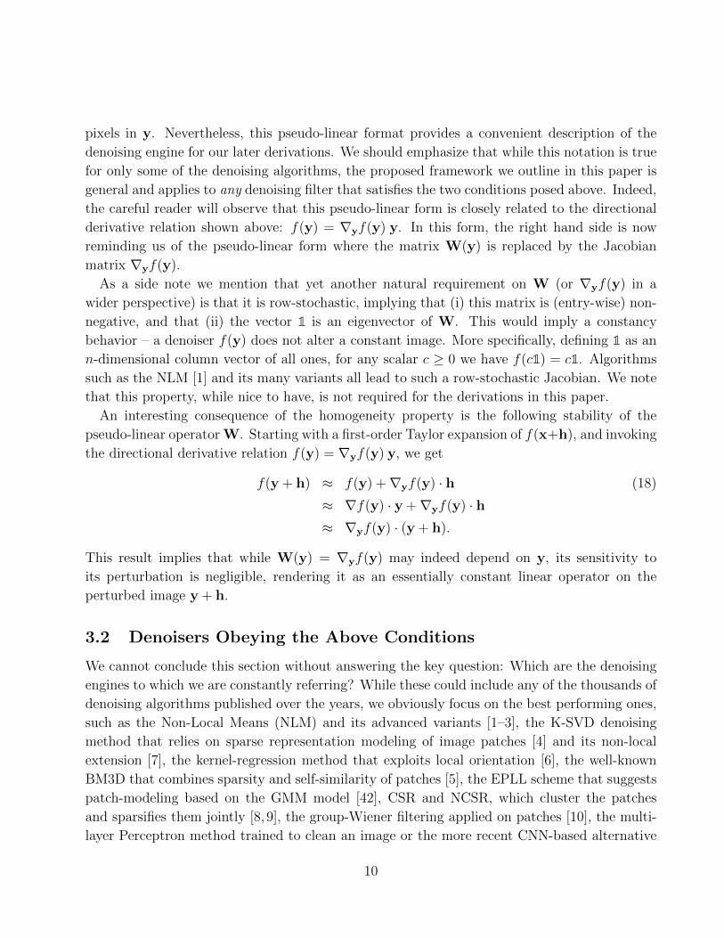
Starting with the homogeneity property, we give an experimental evidence, accompanied

by a theoretical analysis, to substantiate the fulfillment of this property by a series of well-

known denoisers. Figure 1 shows f((1 + ε)x) versus (1 + ε)f(x) as a scatter-plot, tested for

K-SVD, BM3D, NLM, EPLL, and the TNRD. In all these experiments, the image x is set to be

Peppers, ε = 0.01 and σ = 5 (level of noise assumed within f). As can be seen, a tendency to

an equality f((1 + ε)x) ≈ (1 + ε)f(x) is obtained, suggesting that all these are indeed satisfying

the homogeneity property. The deviation from exact equality in each of these tests has been

evaluated as the standard deviation of the difference f((1 + ε)x) − (1 + ε)f(x), leading to

2.95e− 4, 3.38e− 4, 1.38e− 4, 1.46e− 4, 9.51e− 5, respectively. A further discussion on the

homogeneity property from a theoretical perspective is given in Appendix C.

Turning to the passivity condition, a conceptual difficulty is the need to explicitly obtain the

Jacobian of the denoiser in question. Assuming that we overcame this problem somehow and

got ∇xf(x), its spectral radius would be evaluated using the Power-Method [69] that applies

iterations of the form

hk+1 =∇xf(x) · hk‖∇xf(x) · hk‖2

. (19)

The spectral radius itself is easily obtained as

η (∇xf(x)) =hTk+1hk

hTkhk. (20)

In order to bypass the need to explicitly obtain ∇xf(x)hk, we rely on the first order Taylor

expansion again,

f(x + h) = f(x) +∇xf(x) · h, (21)

implying that ∇xf(x) · h ≈ f(x + h)− f(x), which holds true if ‖h‖2 is small enough. Thus,

our alternative Power-Method activates one denoising step per iteration,

hk+1 ≈f(x + hk)− f(x)

‖f(x + hk)− f(x)‖2

. (22)

11

(a) K-SVD (2.95e− 4) (b) BM3D (3.38e− 4) (c) NLM (1.38e− 4)

(d) EPLL (1.46e− 4) (e) TNRD (9.51e− 5)

Figure 1: An empirical evaluation of the homogeneity property. These graphs show f((1 + ε)x)

versus (1 + ε)f(x) as a scatter-plot for K-SVD, BM3D, NLM, EPLL, and the TNRD. Equality

implies satisfaction of the homogeneity, and the numbers in the brackets provide the STD of

the difference. Note that these results were observed on various test images, but shown here

for the image Peppers.

12

The vector hk is normalized in each iteration, and thus ‖hk‖2 = 1. This vector is an image,

and thus the gray values in it must be very small (hk(j)� 1), so as to lead to a sum of squares

to be equal to 1. This agrees with the need for the perturbation x + hk to be small.

This algorithm has been applied to K-SVD, BM3D, NLM, EPLL, and the TNRD (x set to be

the image Cameraman, σ = 5, number of iterations set to give an accuracy of 1e− 5), resulting

all with values smaller or equal to 1, verifying the passivity of these filters.

4 Regularization by Denoising (RED)

4.1 The Image-Adaptive Laplacian

The new and alternative framework we propose relies on a form of an image-adaptive Laplacian

which builds a powerful (empirical) prior that can be used to regularize a variety of inverse

problems. As a place to start and motivate this definition, let’s go back to the description of

the denoiser given in Equation (17), namely4 W(x)x. We may think of this pseudo-linear filter

as one where a set of coefficients (depending on x) are first computed in the matrix W, and

then applied to the image x. From this we can construct the Laplacian form,

ρL(x) =1

2xTL(x)x =

1

2xT (I−W(x))x =

1

2xT [x−W(x)x] . (23)

This definition by itself is not novel, as it is similar to ideas brought up in a series of recent

contributions [48–57]. This expression relies on using an image-adaptive Laplacian – one that

draws its definition from the image itself.

Observing the obtained expression, we note that it can be interpreted as the unnormalized

cross-correlation between the image x and its corresponding residual x −W(x)x. As a prior

expression should give low values for likely images, in our case this would be achieved in one

of two ways (or their combination):

• A small value is obtained for ρL(x) if the residual is very small, implying that the image

x serves as a near fixed-point of the denoising engine, x ≈W(x)x.

• A small value is obtained for ρL(x) if the cross-correlation of the residual to the image itself

is small, a feature that implies that the residual behaves like white noise, or alternatively,

if it does not contain elements from the image itself. Interestingly, this concept has been

harnessed successfully by some denoising algorithms such as the Dantzig-Selector [63]

and by image denoising boosting techniques [52, 64, 65]. Indeed, enforcing orthogonality

between the signal and its treated residual is the underlying force behind the Normal

equations in statistical estimation (e.g. Least Squares and Kalman Filtering).

4Note that we conveniently assume that the prior is applied to the clean image x, a matter that will be

clarified as we dive into our explanations.

13

Given the above prior, we return to the general inverse-problem posed in Equation (6), and

define our new objective,

x = Argminx

`(y,x) +λ

2xT [x−W(x)x] . (24)

The prior expression, while exhibiting a possibly complicated dependency on the unknown x,

is well-defined and clear. Nevertheless, an attempt to apply any gradient-based algorithm for

solving the above minimization task encounters an immediate problem, due to the need to

differentiate W(x) with respect to x. We overcome this problem by observing that W(x)x is

in fact the activation of the image denoising engine on x, i.e., f(x) = W(x)x. This observation

inspires the following more general definition of the Laplacian regularizer, which is the prime

message of this paper:

ρL(x) =1

2xT [x− f(x)] . (25)

This is the Regularization by Denoising (RED) paradigm that this work advocates. In this

expression, the residual is defined more generally for any filter f(x) even if it can not be

written in the familiar (pseudo-)linear form. Note that all the preceding intuition about the

meaning of this prior remains intact; namely, the value is low if the cross-correlation between

the image and its denoising residual is small, or if the residual itself is small due to x being a

fixed point of f .

Surprisingly, while this expression is more general, it leads to a better-managed optimization

problem due to the careful properties we have outlined in Section 3 on our denoising engines

f . The overall energy functional to minimize is

E(x) = `(y,x) +λ

2xT (x− f(x)) , (26)

and the gradient of this expression is readily available by

∇xE(x) = ∇x`(y,x) +λ

2∇x

{xT (x− f(x))

}(27)

= ∇x`(y,x) +λ

2∇xx

Tx− λ

2∇x

[xTf(x)

]= ∇x`(y,x) + λx− λ

2[f(x) +∇xf(x)x] .

Based on our prior assumption regarding the availability of a directional derivative for the

denoising engine, the term ∇xf(x)x can be replaced5 by ∇xf(x) x = f(x), based on Equation

(14), implying that the gradient expression is further simplified to be

∇xE(x) = ∇x`(y,x) + λx− λf(x) = ∇x`(y,x) + λ(x− f(x)), (28)

5A better approximation can be applied in which we replace ∇xf(x)x by the difference (f((1+ε)x)−f(x))/ε,

but this calls for two activations of the denoising engine per gradient evaluation.

14

requiring only one activation of the denoising engine for the gradient evaluation. Interestingly,

if we bring back now the pseudo-linear interpretation of the denoising engine, the gradient

would be the residual, just as posed above, implying that

∇xE(x) = ∇x`(y,x) + λ(x−W(x)x). (29)

Observe that this is a non-trivial derivation of the gradient of the original penalty function

posed in Equation (24).

4.2 Deploying the Denoising Engine for Solving Inverse Problems

In the discussion above we have seen that the gradient of the energy functional to minimize

(given in Equation (26)) is easily computable, given in Equation (28). We now turn to show

several options for using this in order to solve a general inverse problem. Common to all these

methods is the fact that the eventual algorithm is iterative, in which each step is composed of

applying the denoising engine (once or more), accompanied by other simpler calculations. In

Figures 2, 3, and 4 we present pseudo-code for several such algorithms, all in the context of

handling the case in which the likelihood function is given by `(y,x) = ‖Hx− y‖22/2σ

2.

• Gradient Descent Methods: Given the gradient of the energy function E(x), the

Steepest-Descent (SD) is the simplest option that can be considered, and it amounts to

the update formula

xk+1 = xk − µ∇x E(x)|xk (30)

= xk − µ[∇x `(y,x)|xk + λ(xk − f(xk))

].

Figure 2 describes this algorithm in more details.

A line-search can be proposed in order to set µ dynamically per iteration, but this is

necessarily more involved. For example, in the case of the Armijo rule, it requires a

computation of the above gradient gk and then assessing the energy E(xk − µgk) for

different values of µ in a retracting fashion, each of which calling for a computation of

the denoising engine once.

One could envision using the Conjugate-Gradient (CG) to speed this method, or better

yet, applying the Sequential Subspace Optimization (SESOP) algorithm [70]. SESOP

holds the current gradient and the last several update directions as the columns of a

matrix Vk (referring to the kth iteration), and seeks the best linear combination of these

columns as an update direction to the current solution, namely xk+1 = xk +Vkαk. When

restricted to have only one column, this reduces to a simple SD with line-search. When

using two columns, it has the flavor (and strength) of CG, and when using more columns,

15

this method can lead to much faster convergence in non-quadratic problems. The key

points of SESOP are (i) The matrix V is updated easily from one iteration to another by

discarding the last direction, bringing in the last one, and adding the new gradient; and

(ii) The unknown weights vector αk is low-dimensional, and thus updating it can be done

using a Newton method. Naturally, one should evaluate the first and second derivatives of

the penalty function w.r.t. αk, and these will leverage the relations established above. We

shall not dive deeper into this option because it will not be included in our experiments.

One possible shortcoming of the gradient approach (in all its manifestations) is the fact

that per activation of the denoising engine, the likelihood is updated rather mildly as a

simple step toward the current log-likelihood gradient. This may imply that the overall

algorithm will require many iterations to converge. The next two methods propose a way

to overcome this limitation, by treating the log-likelihood term more “aggressively”.

Objective: Minimize E(x) = 12σ2 ‖Hx− y‖22 + λ

2xT (x− f(x))

Input: Supply the following ingredients and parameters:

– Regularization parameter λ,

– Denoising algorithm f(·) and its noise level σf ,

– Log-Likelihood parameters: H and σ, and

– Number of iterations N .

Initialization:

• Set x0 = y.

• Set µ = 21/σ2+λ

.

Loop: For k = 1, 2 . . . , N do:

• Apply the denoising engine, xk = fσf (xk−1).

• Update the solution by xk = xk−1 − µ[

1σ2 H

T (Hxk−1 − y) + λ(xk−1 − xk)].

End of Loop

Result: The output of the above algorithm is xN .

Figure 2: The proposed scheme (RED) via the steepest descent method.

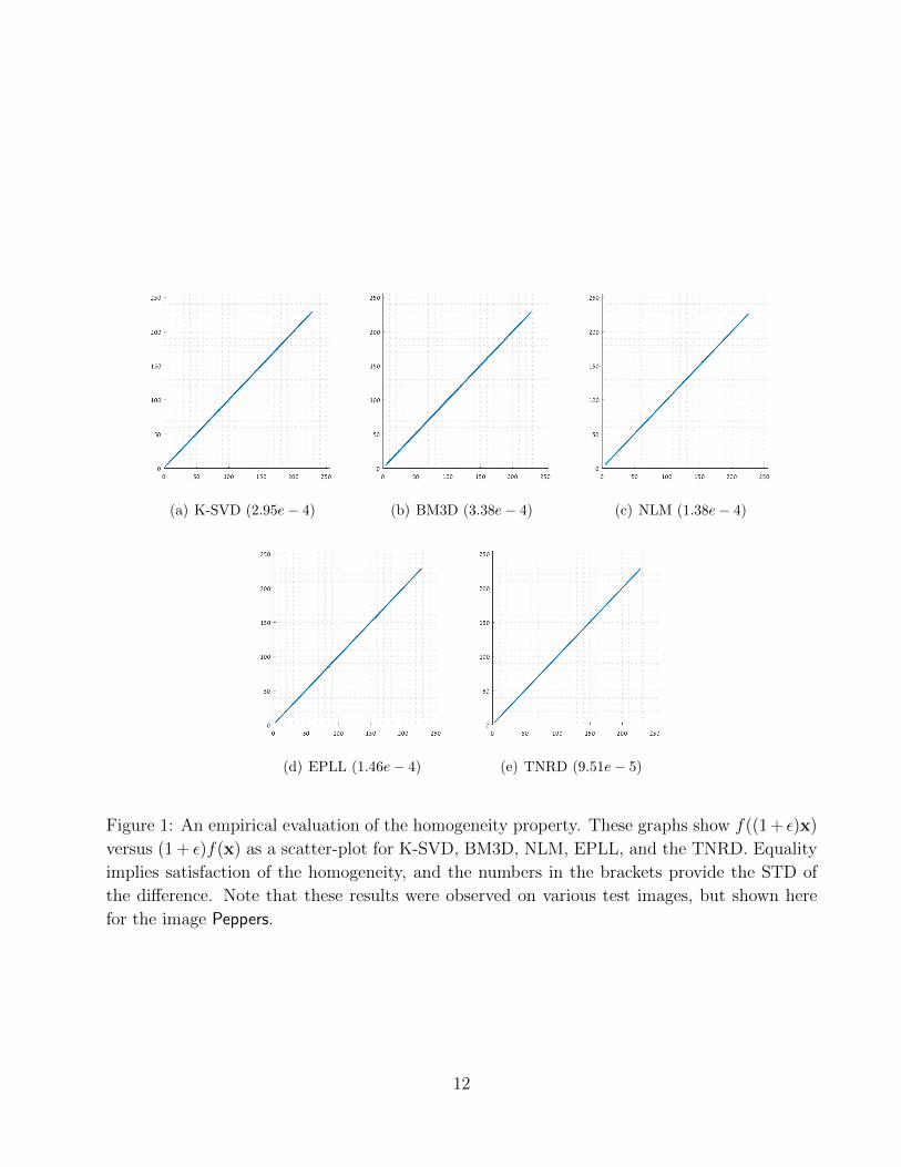
• ADMM: Addressing the optimization task given in Equation (26), we can imitate the

path taken by the P 3 scheme, and apply variable splitting and ADMM. The steps would

follow the description given in Section 2 almost exactly, with one major difference – the

prior in our case is explicit, and therefore, the stage termed “update of v” would become

v = Argminv

λ

2vT (v− f(v)) +

β

2‖v− x− u‖2

2. (31)

16

Rather than applying an arbitrary denoising engine to compute v as a replacement to

the actual minimization, we should target this minimization directly by some iterative

scheme. For example, setting the gradient of the above expression to zero leads to the

equation

λ(v− f(v)) + β(v− x− u) = 0, (32)

which can be solved iteratively using the fixed-point strategy, by

λ(vj − f(vj−1)) + β(vj − x− u) = 0 (33)

→ vj =1

β + λ(λf(vj−1 + β(x + u)) .

This means that our approach in this case is computationally more expensive, as it will

require several activations of the denoising engine. However, a common approach to speed

up the convergence (in terms of runtime) of the ADMM is called “early termination” [58],

suggesting to approximate the solution of the v-update stage. We found this approach

useful for our setting, especially because the application of a denoiser is computationally

expensive. To this end, we may choose to apply only one iteration of the iterative process

described in Equation (33), which amounts to one operation of a denoising algorithm.

Figure 3 describes this specific algorithm in more details. If one changes all Part 2 (in

Figure 3) with the computation vk = f1/√β(z∗), we obtain the P 3 scheme for the same

choice of the denoising engine. While this difference is quite delicate, we should remind

the reader that (i) this bridge between the two approaches is valid only when we deploy

ADMM on our scheme, and (ii) as opposed to the P 3 method, our method is guaranteed

to converge to the global optimum of the overall penalty function, as will be described

hereafter.

We should point out that when using the ADMM, the update of x applies an aggressive in-

version of the log-likelihood term, which is followed by the above optimization task. Thus,

the shortcoming mentioned above regarding the lack of balance between the treatments

given to the likelihood and the prior is mitigated.

• Fixed-Point Strategy: An appealing alternative to the above exists, obtained via the

fixed-point strategy. As our aim is to find x that nulls the gradient, this could be posed

as an implicit equation to be solved directly,

∇x`(y,x) + λ(x− f(x)) = 0. (34)

Using the fixed-point strategy, this could be handled by the iterative formula

∇x`(y,xk+1) + λ(xk+1 − f(xk)) = 0. (35)

17

Objective: Minimize E(x) = 12σ2 ‖Hx− y‖22 + λ

2xT (x− f(x))

Input: Supply the following ingredients and parameters:

– Regularization parameter λ,

– Denoising algorithm f(·) and its noise level σf ,

– Log-Likelihood parameters: H and σ,

– Number of outer and inner iterations, N , m1, and m2, and

– ADMM coefficient β.

Initialization: Set x0 = y, v0 = y, and u0 = 0.

Outer Loop: For k = 1, 2 . . . , N do:

Part 1: Solve xk = Argminz

12σ2 ‖Hz− y‖22 + β

2‖z− vk−1 + uk−1‖22 by

• Initialization: z0 = xk−1, and define z∗ = vk−1 − uk−1.

• Inner Iteration: For j = 1, 2 . . . ,m1 do:

− Compute the gradient ej = 1σ2 H

T (Hzj−1 − y) + β(zj−1 − z∗).

− Compute rj = 1σ2 H

THej + βej .

− Compute the step size µ = eTj ej/eTj rj .

− Update the solution by zj = zj−1 + µej .

− Project the result to the interval [0, 255].

• End of Inner Loop

• Set xk = zm1 .

Part 2: Solve vk = Argminz

λzT (z− fσf (z)) + β2‖z− xk − uk−1‖22 by

• Initialization: z0 = vk−1, and define z∗ = xk + uk−1.

• Inner Iteration: For j = 1, 2 . . . ,m2 do:

− Apply the denoising engine, zj = fσf (zj−1).

− Compute the gradient zj = 1β+λ

(λzj + βz∗).

• End of Inner Loop

• Set vk = zm2 .

Part 3: Update uk = uk−1 + xk − uk.

End of Outer Loop

Result: The output of the above algorithm is xN .

Figure 3: The proposed scheme (RED) via the ADMM method.

18

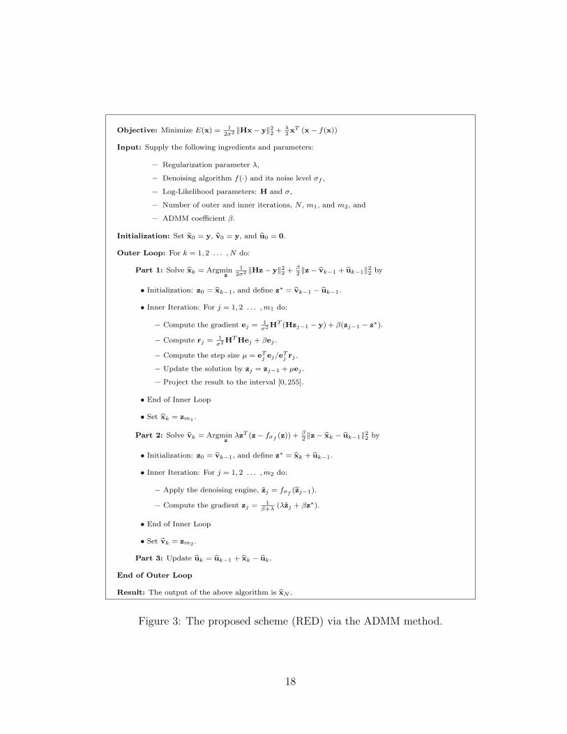
As an example, in the case of linear degradation model and Gaussian white additive noise,

this equation would be

1

σ2HT (y−Hxk+1) + λ(xk+1 − f(xk)) = 0, (36)

leading to the recursive update relation

xk+1 =

[1

σ2HTH + λI

]−1 [1

σ2HTy + λf(xk)

]. (37)

This formula suggests one activation of the denoising per iteration, followed by what

seems to be a plain Wiener filtering computation6. The matrix inversion itself could be

done in the Fourier domain for block-circulant H, or iteratively using for example, the

Richardson algorithm: Defining

A =1

σ2HTH + λI and b =

1

σ2HTy + λf(xk), (38)

our goal is to solve the linear system Ax = b. This is achieved by a variant of the SD

method7, xj+1 = xj − µ(Axj − b) = xj − µej, where we have defined ej = Axj − b. By

setting the step size to be µj = eTj Aej/eTj ATAej, we greedily optimize the potential of

each iteration.

Convergence of the above algorithm is guaranteed since∥∥∥∥∥[

1

σ2HTH + λI

]−1

λ∇xf(xk)

∥∥∥∥∥ < 1. (39)

This approach, similarly to the ADMM, has the desired balance mentioned above between

the likelihood and the regularization terms, matching the efforts dedicated to both. A

pseudo-code describing this algorithm appears in Figure 4.

A basic question that has not been discussed so far is how to set the parameters of f(x) in

defining the regularization term. More specifically, assuming that the denoising engine depends

on one parameter – the noise standard-deviation σf – the question is which value to use. While

one could envision using varying values as the iterations progress and the outcome improves,

the approach we take in this work is to set this parameter to be a small and fixed value.

Our intuition for this choice is the desire to have a clear and fixed regularization term, which

in turn implies a clear cost function to work with. Furthermore, the prior we propose should

encapsulate in it our desire to get to a final image that is a stable point of such a weak denoising

engine, x ≈ f(x). Clearly, more work is required to better understand the influence of this

parameter and its automatic setting.

6Note that Equation (33) refers to the same problem posed here under the choice H = I and β = 1/σ2.7All this refer to a specific iteration k within which we apply inner iterations to solve the linear system, and

thus the use of the different index j.

19

Objective: Minimize E(x) = 12σ2 ‖Hx− y‖22 + λ

2xT (x− f(x))

Input: Supply the following ingredients and parameters:

• Regularization parameter λ,

• Denoising algorithm f(·) and its noise level σf ,

• Log-Likelihood parameters: H and σ, and

• Number of outer and inner iterations, N and m.

Initialization: x0 = y.

Outer Loop: For k = 1, 2 . . . , N do:

• Apply the denoising engine, xk = fσf (xk−1).

• Solve Az = b for A = 1σ2 H

TH + λI and b = 1σ2 H

Ty + λxk

- Initialization: z0 = xk.

- Iterate: For j = 1, 2 . . . ,m do:

• Compute the residual rj = Azj−1 − b.

• Compute the vector ej = Arj .

• Compute the optimal step µ = rTj ej/eTj ej .

• Update the solution by zj = zj−1 + µ · rj .

• Project the result to the interval [0, 255].

- End of Inner Loop

- Set xk = zm.

End of Outer Loop

Result: The output of the above algorithm is xN .

Figure 4: The Proposed Scheme (RED) via the fixed-point method.

20

5 Analysis

5.1 Convexity

Is our proposed regularization function ρL(x) convex? At first glance, this may seem like too

much to expect. Nevertheless, it appears that for reasonably performing denoising engines

obeying the conditions posed in Section 3, this is exactly the case. For the function ρL(x) =

xT (x − f(x)) to be convex, we should demand that the second derivative is a positive semi-

definite matrix [67]. We have already seen that the first derivative is simply x − f(x), which

leads to the conclusion that the second derivative is given by I−∇xf(x).

As already mentioned earlier, in the context of some algorithms such as the NLM and the

K-SVD, this is associated with the Laplacian I −W(x), and it is positive semi-definite if W

has all its eigenvalues in the range8 [0, 1]. This is indeed the case for the NLM filter [1], the

K-SVD-denoising algorithm [57], and many other denoising engines.

In the wider context of general image denoising engines, convexity is assured if the Jacobian

∇xf(x) of the denoising algorithm is stable, as indeed required in Condition 2 in Section 3,

η(∇xf(x)) ≤ 1. In this case we have that ρL(·) is convex, and this implies that if the log-

likelihood expression is convex as well, the proposed scheme is guaranteed to converge to the

global optimum of our cost function in Equation (6). In this respect the proposed algorithm is

superior to the P 3 scheme in its most general form, which at best is known to get to a stable-

point [30, 32]. Furthermore, this result may seem similar to the one posed in [33, 38], as our

two conditions for global convergence are homogeneity and passivity of f , while in these papers

the requirements are passivity of f , along with a convex energy functional whom f minimizes.

The second condition – having a convex origin to derive f(x) – is in fact more restrictive than

demanding homogeneity, as it is unclear which of the known denoisers meet this requirement.

5.2 An Alternative Prior

In Section 4 we motivated the choice of the proposed prior by the desire to characterize the

unknown image x as one that is not affected by the denoising algorithm, namely, x ≈ f(x).

Rather than taking the route proposed, we could have suggested a prior of the form

ρQ(x) = ‖x− f(x)‖22. (40)

This prior term makes sense intuitively, being based on the same desire to see the denoising

residual being small. Indeed, this choice is somewhat related to the option we chose since

ρQ(x) = ‖x− f(x)‖22 = ρL(x) + f(x)T (f(x)− x), (41)

8We could in fact allow negative eigenvalues for W, but this is unnatural in the context of denoising.

21

suggesting a symmetrization of our own expression.

In order to understand the deeper meaning of this alternative, we resort again to the pseudo-

linear denoisers, for which this prior is nothing but

ρQ(x) = ‖x−W(x)x‖22 = xT (I−W(x))T (I−W(x))x. (42)

This means that rather than regularizing with the Laplacian, we do so with its square. While

this is a worthy possibility which has been considered in the literature under the term “fourth

order regularization” [71], it is known to be more delicate. We leave this and other possibilities

of formulating the regularization with the use of f(x) for future work.

5.3 When is Plug-and-Play-Prior = RED ?

In Section 4 we described the use of ADMM as one of the possible avenues for handling our

proposed regularization. When handling the inverse problem posed in Equation (26) with

ADMM, we have shown that the only difference between this and the P 3 scheme resides in

the update stage for v. Here we aim to answer the following question: Assuming that the

numerical algorithm used is indeed the ADMM, under what conditions would the two methods

(P 3 and ours) become equivalent? The answer to this question resides in the optimization task

for updating v, which is a denoising task. Thus, purifying this question, our goal is to find

conditions on f(·) and λ such that the two treatments of this update stage coincide. Starting

from our approach, we would seek the solution of

x = Argminx

β

2‖x− y‖2

2 +λ

2xT (x− f(x)) , (43)

or, putting it in terms of nulling the gradient of this energy, require

β(x− y) + λ(x− f(x)) = 0. (44)

The x that is the solution of this equation is our updated image. On the other hand, the

P 3 scheme would propose to simply compute9 x = f(y) as a replacement to this minimization

task. Therefore, for the two methods to coincide, we should demand that the gradient expression

posed above is solved for the choice of the P 3 scheme, namely,

β(f(y)− y) + λ(f(y)− f(f(y))) = 0, (45)

or posed slightly different,

f(y)− f(f(y)) =β

λ(y− f(y)). (46)

9A delicate matter not considered here is that P 3 may apply 1cf(cy) in order to tune to a specific noise level.

We assume c = 1 for simplicity.

22

This means that the denoising residual should remain the same (up to a constant) for the first

activation of the denoising engine y − f(y), and the second one applied on the filtered image

f(y).

In order to get a better intuition towards this result, let’s return to the pseudo-linear case,

f(y) = Wy with the assumption that W is a fixed and diagonalizable matrix. Plugged into

the above condition, this gives

Wy−W2y =β

λ(y−Wy), (47)

or posed differently, (β

λI−W

)(I−W) y = 0. (48)

As the above equation should hold true for any image y, we require(β

λI−W

)(I−W) = 0. (49)

Without loss of generality, we can assume that W is diagonal, after multiplying the above

equation from the left and right by the diagonalizing matrix. With this simplification in mind,

we now consider the eigenvalues of W, and the above equation implies that exact equivalence

between our scheme and the P 3 one is obtained only if our denoising engine has eigenvalues

that are purely 1’s, or β/λ. Clearly, this is a very limiting case, which suggests that for all

other cases, the two methods are likely to differ.

Interestingly, the above analysis is somewhat related to the one given in [31]. Both [31]

and our treatment assume that the actual applied denoising engine is f(y) = Wy within

the ADMM scheme. While we ask for the conditions on W to fit our regularization term

xT (x−Wx), the author of [31] seeks the actual form of the prior to match this step, reaching

the conclusion that the prior should be xT (I −W)W†x. Bearing in mind that the conditions

we get for the equivalence between the two methods are too restricting and rarely met, the

result in [31] shows the actual gap between the two methods: While we regularize with the

expression xT (I−W)x, an equivalence takes place only if the P 3 modifies this to involve W†,

getting a far more complicated and less natural term.

Just before we conclude this section, we turn briefly to discuss the computational complexity

of the proposed algorithm and its relation to the complexity of the P 3 scheme. Put very

simply, RED and P 3 are roughly of the same computational cost. This is the case when RED

is deployed via ADMM and assuming only one iteration in the update of v, as shown above.

Similarly, when using the fixed-point option, RED has the same cost as P 3 per iteration.

To conclude, we must state that this paper is about a more general framework rather than

a comparison to the P 3. Indeed, one could consider this work as an attempt to provide more

23

solid mathematical foundations for methods like the P 3. In addition, when comparing P 3 and

RED, one can identify several major differences that are far more central than the complexity

issue, such as (1) a lack of a clear objective function that P 3 serves, while our scheme has a very

well-defined penalty; (2) the inability to claim much in terms of convergence of the P 3, while

our penalty is shown to be convex; (3) the complications of tuning the P 3 algorithm, which is

very different from the experience we show with RED.

6 Results

In this section we compare the performance of the proposed framework to the P 3 approach,

along with various other leading algorithms that are designed to tackle the image deblurring and

super-resolution problems. To this end, we plug two substantially different denoising algorithms

into the proposed scheme. The first is the (simple) median filter, which surprisingly turns out

to act as a reasonable regularizer to our ill-posed inverse problems. This option is brought as

a core demonstration of the idea that an arbitrary denoiser can be deployed in RED without

difficulties. The second denoising engine we use is the state-of-the-art Trainable Nonlinear

Reaction Diffusion (TNRD) [20] method. This algorithm trains a nonlinear reaction-diffusion

model in a supervised manner. As such, in order to treat different restoration problems, one

should re-train the underlying model for every specific task – something we aim to avoid. In the

experiments below we build upon the published pre-trained model by the authors of TNRD,

tailored to denoise images that are contaminated by white Gaussian noise with a fixed10 noise-

level, which is equal to 5. Leveraging this, we show how state-of-the-art deblurring and super-

resolution results can be achieved simply by integrating the TNRD denoiser in RED. In all the

experiments that follow, the parameters were manually set in order to enable each method to

get its best possible results over the subset of images tested.

6.1 Image Deblurring

In order to have a fair comparison to previous work, we follow the synthetic non-blind deblurring

experiments conducted in the state-of-the-art work that introduced the Non-locally Centralized

Sparse Representation (NCSR) algorithm [9], which combines the self-similarity assumption [1]

with the sparsity-inspired model [68]. More specifically, we degrade the test images, supplied

by the authors of NCSR, by convolving them with two commonly used point spread functions

(PSF); the first is a 9 × 9 uniform blur, and the second is a 2D Gaussian function with a

standard deviation of 1.6. In both cases, an additive Gaussian noise with σ =√

2 is then added

to the blurred images. Similarly to NCSR, restoring an RGB image is done by converting it to

10In order to handle an arbitrary noise-level, σf , we rely on the following relation fσf(y) = 1

cf5(c ·y), where

c = 5/σf .

24

the YCbCr color-space, applying the deblurring algorithm on the luminance channel only, and

then converting the result back to the RGB domain.

Table 1 provides the restoration performance of the three RED schemes – the steepest-

descent (SD), the ADMM, and the fixed-point (FP) methods – along with the results of the11

P 3, the state-of-the-art NCSR and IDD-BM3D [27], and two additional baseline deblurring

methods [72, 73]. For brevity, only the steepest-descent scheme is presented when considering

the basic median filter as a denoiser. The performance is evaluated using the Peak Signal

to Noise Ratio (PSNR) measure, higher is better, computed on the luminance channel of the

ground-truth and the estimated image. The parameters of the proposed approach, as well as

the ones of the P 3, are tuned to achieve the best performance on this dataset; in the case

of the TNRD denoiser, these are depicted in Table 2 and 3, respectively. In the setting of

the median filter, which extracts the median value of a 3 × 3 window, we choose to run the

suggested steepest-descent scheme for N = 400 iterations with λ = 0.12 for the uniform PSF,

and N = 200 with λ = 0.225 for the Gaussian PSF.

Image Butterfly Boats C. Man House Parrot Lena Barbara Starfish Peppers Leaves Average

Deblurring: Uniform kernel, σ =√2

Total Variation [72] 28.37 29.04 26.82 31.99 29.11 28.33 25.75 27.75 28.43 26.49 28.21IDD-BM3D [27] 29.21 31.20 28.56 34.44 31.06 29.70 27.98 29.48 29.62 29.38 30.06ASDS-Reg [73] 28.70 30.80 28.08 34.03 31.22 29.92 27.86 29.72 29.48 28.59 29.84

NCSR 29.68 31.08 28.62 34.31 31.95 29.96 28.10 30.28 29.66 29.98 30.36P3-TNRD 30.32 31.19 28.73 33.90 31.86 30.13 27.21 30.27 30.11 30.08 30.38

RED: SD-Median Filter 26.10 28.03 25.57 29.81 28.67 27.29 25.62 27.84 27.40 25.45 27.18RED: SD-TNRD 30.20 31.20 28.67 33.83 31.62 29.98 27.35 30.47 30.10 29.72 30.31

RED: ADMM-TNRD 30.40 31.12 28.71 33.77 31.86 30.03 27.27 30.58 30.11 30.12 30.40RED: FP-TNRD 30.41 31.12 28.76 33.76 31.83 30.02 27.27 30.57 30.12 30.13 30.40

Deblurring: Gaussian kernel, σ =√2

Total Variation [72] 30.36 29.36 26.81 31.50 31.23 29.47 25.03 29.65 29.42 29.36 29.22IDD-BM3D [27] 30.73 31.68 28.17 34.08 32.89 31.45 27.19 31.66 29.99 31.4 30.92ASDS-Reg [73] 29.83 30.27 27.29 31.87 32.93 30.36 27.05 31.91 28.95 30.62 30.11

NCSR [9] 30.84 31.49 28.34 33.63 33.39 31.26 27.91 32.27 30.16 31.57 31.09P3-TNRD 31.73 31.67 28.08 33.95 33.43 31.52 27.11 32.71 30.94 32.18 31.33

RED: SD-Median Filter 29.02 30.01 26.45 31.59 31.32 30.00 25.02 30.29 28.53 28.69 29.09RED: SD-TNRD 31.57 31.53 28.31 33.71 33.19 31.47 26.62 32.46 29.98 31.95 31.08

RED: ADMM-TNRD 31.66 31.55 28.31 33.73 33.33 31.40 26.76 32.49 30.48 31.93 31.16RED: FP-TNRD 31.66 31.55 28.38 33.74 33.33 31.39 26.76 32.49 30.51 31.93 31.17

Table 1: Deblurring results measured in PSNR [dB] and evaluated on the set of images provided

by the authors of NCSR [9]. The P 3 and RED build upon the TNRD [20] as the denoising

engine. We also provide the results obtained by integrating the median filter with the steepest-

descent RED scheme. PSNR scores being less than 0.01[dB] away from the highest result are

highlighted. Note that the P 3 does not converge when setting the TNRD to be the denoising

algorithm. Therefore, we run the P 3 for a fixed number of iterations, chosen to achieve the

best PSNR on average (otherwise the restoration quality would be significantly inferior). Please

refer to Figure 10 and Section 6.3 for more details regarding the sensitivity of the P 3 to the

choice of parameters.

Several remarks are to be made with regard to the obtained results. When the image is

degraded by a Gaussian blur kernel, integrating the median filter in the proposed framework

leads to a surprising restoration performance that is similar to the total variation deblurring [72].

11We note that P 3 using TNRD has never appeared in an earlier publication, and it is brought here in order

to let P 3 perform as best as it possibly can.

25

PSFProposed approach: Deblurring

ParameterSteepest Fixed

ADMMDescent Point

Un

iform

N 1500 200 200σf 3.25 3.25 3.25λ 0.02 0.02 0.02m1 – closed-form using FFT closed-form using FFTm2 – – 1β – – 0.001

Gau

ssia

n

N 1500 200 200σf 4.1 4.1 4.1λ 0.01 0.01 0.01m1 – closed-form using FFT closed-form using FFTm2 – – 1β – – 0.001

Table 2: The set of parameters being used in our framework, leading to the deblurring results

reported in Table 1 when plugging the TNRD [20] denoiser.

PSFP 3: Deblurring

Parameter Value

Un

iform

N 200α 1.02β0 0.0007βk αk · β0λ 512 · β0σf

√λ/βk

Gau

ssia

n

N 200α 1.02β0 0.0007βk αk · β0λ 320 · β0σf

√λ/βk

Table 3: The set of parameters being used by the P 3 method, leading to the deblurring results

reported in Table 1 when plugging the TNRD [20] denoiser.

26

101 102 103

Iteration

0.2

0.4

0.6

0.8

1

1.2

1.4

1.6

1.8

Cos

t

#105

SDADMM: m

2=1

ADMM: m2=3

FP

(a) RED, Denoising Engine: Median Filter

101 102 103

Iteration

1.3

1.4

1.5

1.6

1.7

1.8

1.9

2

2.1

2.2

Cos

t

#104

SDADMM: m

2=1

ADMM: m2=3

FP

(b) RED, Denoising Engine: TNRD

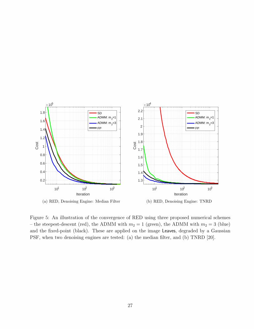
Figure 5: An illustration of the convergence of RED using three proposed numerical schemes

– the steepest-descent (red), the ADMM with m2 = 1 (green), the ADMM with m2 = 3 (blue)

and the fixed-point (black). These are applied on the image Leaves, degraded by a Gaussian

PSF, when two denoising engines are tested: (a) the median filter, and (b) TNRD [20].

27

(a) Ground Truth (b) Input 20.83dB (c) RED: SD-Median filter

25.87dB

(d) NCSR 28.39dB (e) P 3-TNRD 28.43dB (f) RED: FP-TNRD 28.82dB

Figure 6: Visual comparison of deblurring a cropped area from the image Starfish, degraded by

a uniform PSF, along with the corresponding PSNR [dB] score.

28

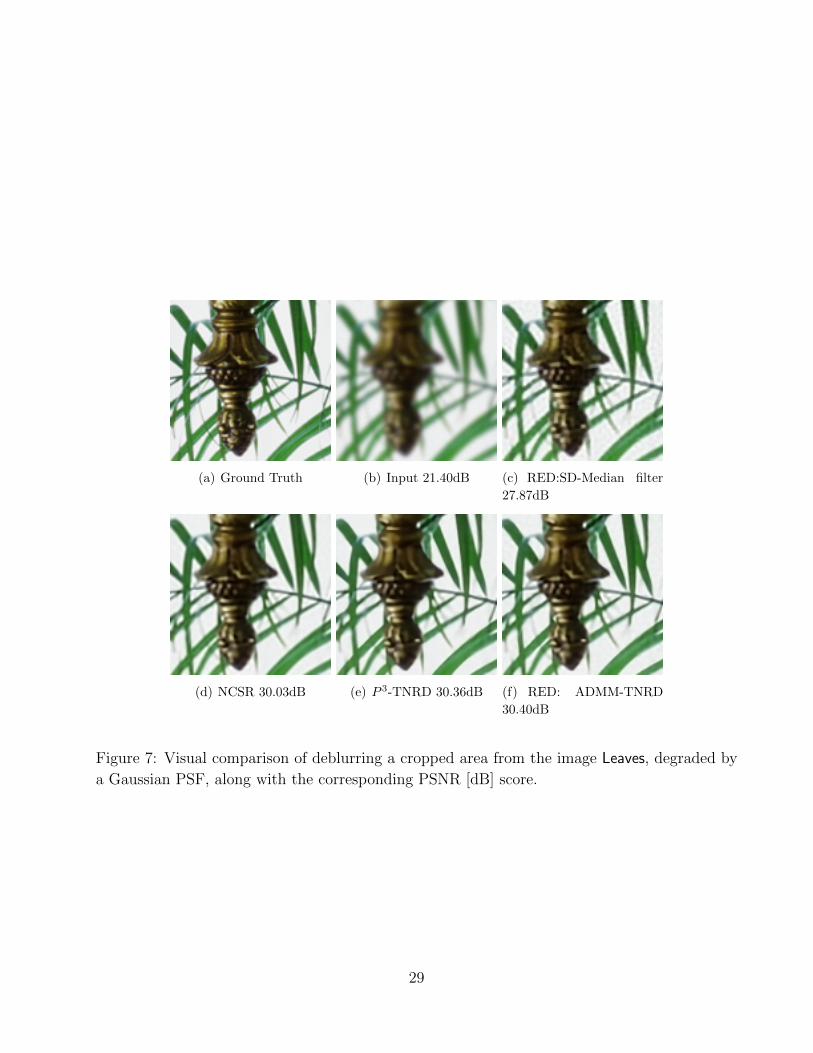
(a) Ground Truth (b) Input 21.40dB (c) RED:SD-Median filter

27.87dB

(d) NCSR 30.03dB (e) P 3-TNRD 30.36dB (f) RED: ADMM-TNRD

30.40dB

Figure 7: Visual comparison of deblurring a cropped area from the image Leaves, degraded by

a Gaussian PSF, along with the corresponding PSNR [dB] score.

29

Furthermore, by choosing the state-of-the-art TNRD to be our denoising engine we achieve

results that are competitive with the impressive NCSR and IDD-BM3D methods, which are

specifically designed to tackle the deblurring task. Notice that the three versions of the proposed

framework obtain a similar PSNR score. However, while the ADMM and the fixed-point variants

are of similar complexity, the steepest-descent requires many more steps to converge and thereby

more applications of the denoiser. As our last observation, based on the obtained results we

conclude that the proposed approach is equivalent in quality to the alternative P 3 framework.

However, tuning the parameters of the proposed algorithm is significantly simpler than the ones

of the P 3; while in the P 3 the parameters should be modified throughout the iterations, in our

approach these are always fixed (refer to Section 6.3 for a broader discussion).

An illustration of the convergence of the proposed approach using the three different numer-

ical schemes (steepest-descent, ADMM, and fixed-point) and the two denoisers (median filter,

and TNRD) is given in Figure 5. As can be observed, the three algorithms indeed converge, but

at different rates; the steepest-descent is the slowest, while the ADMM is the fastest. The fixed-

point strategy is slightly slower than the ADMM alternative, but requires only one application

of the denoiser per iteration while the ADMM demands m2 = 3 such operations. However,

when comparing the fixed-point to the ADMM with the setting m2 = 1 (now both have the

same computational cost) we observe that the fixed-point is faster.

The above discussion is also supported visually in Figure 6 and 7, comparing the proposed

method to the P 3 and the NCSR both for uniform and Gaussian PSF. As can be seen, by

plugging the median filter into RED we improve the quality of the blurry image, yet the gap

in performance between this simplistic approach and the state-of-the-art is substantial. Once

relying on the TNRD, we obtain an efficient deblurring machine that has comparable results

to P 3, and both are competitive or even slightly better than the NCSR.

6.2 Image Super-Resolution

Similarly to the previous subsection, we imitate the super-resolution experiments done in [9].

To this end, a low-resolution image is generated by blurring the ground-truth high-resolution

one with a 7× 7 Gaussian blur kernel with standard deviation 1.6, followed by down-sampling

by a factor of 3 in each axis. Next, white Gaussian noise of standard deviation 5 is added to

the low-resolution images. The upscaling of an RGB image is done by transforming it first to

the YCbCr color-space, super-resolving the luminance channel using the proposed approach (or

the baseline methods), while the chroma channels are upscaled by bicubic interpolation. Lastly,

the outcome is converted back to the RGB color-space.

In terms of PSNR, Table 4 presents the restoration performance of the three variants of

the proposed approach in addition to the ones of the P 3, the NCSR and the ASDS-Reg [73]

algorithms. Similarly to the deblurring case, the PSNR is computed on the luminance channel

30

only. In the case of the TNRD denoiser, the parameters that are used in our approach and in

the P 3 are listed in Table 5 and 6, respectively. In the simpler case of the median filter (defined

by a 3× 3 window), the number of iterations of the proposed steepest-descent algorithm is set

to N = 50 with a parameter λ = 0.0325.

Super-Resolution, scaling = 3, σ =√2

Image Butterfly flower Girl Parth. Parrot Raccoon Bike Hat Plants AverageBicubic 20.74 24.74 29.61 24.04 25.43 26.20 20.75 27.00 27.62 25.13

ASDS-Reg [73] 26.06 27.83 31.87 26.22 29.01 28.01 23.62 29.61 31.18 28.16NCSR [9] 26.86 28.08 32.03 26.38 29.51 28.03 23.80 29.94 31.73 28.48

P3-TNRD 27.13 28.23 32.08 26.50 29.65 27.95 24.04 30.30 31.78 28.63RED: SD-Median Filter 24.44 27.24 31.13 25.80 27.76 27.65 22.89 28.69 30.24 27.32

RED: SD-TNRD 27.37 28.23 32.08 26.54 29.43 27.98 24.04 30.36 31.79 28.65RED: ADMM-TNRD 27.22 28.24 32.08 26.51 29.41 27.97 23.96 30.35 31.77 28.61

RED: FP-TNRD 27.26 28.24 32.08 26.52 29.42 27.97 23.97 30.35 31.77 28.62

Table 4: Super-resolution results, measured in terms of PSNR [dB] and evaluated on the set of

images provided by the authors of NCSR [9]. The P 3 and ours steepest-descent (SD), ADMM,

and fixed-point (FP) methods build upon the TNRD [20] as the denoising engine. We also

provide the results obtained by integrating the median filter in the steepest-descent scheme.

PSNR scores being less than 0.01[dB] away from the highest result are highlighted. Similarly

to the deblurring case, the P 3 does not converge here as well. Therefore, we run it for a fixed

number of iterations, manually tuned to achieve the highest PSNR on average. This behavior

is demonstrated in detail in Figure 10, and discussed in Section 6.3.

Proposed approach: Super-Resolution

ParameterSteepest Fixed

ADMMDescent Point

N 1500 200 200σf 3 3 3λ 0.008 0.008 0.008m1 – 200 (until convergence) 200 (until convergence)m2 – – 1β – – 0.001

Table 5: The set of parameters being used in our framework, leading to the super-resolution

results reported in Table 4 when plugging the TNRD [20] denoiser.

Interestingly, when setting the median filter to be our denoising engine we get a 2.19dB im-

provement (on average) over the bicubic interpolation. Alternatively, when choosing a stronger

denoiser such as the TNRD, we achieve state-of-the-art results. Notably, the P 3 and the three

variants of the proposed approach lead to similar restoration performance, consistent with the

observation that was made in the context of the deblurring problem. These support once again

the claim that our framework is a tangible alternative to the P 3. Figure 8 and 9 visually

compare the proposed method to the P 3 and also to the state-of-the-art NCSR. As shown, the

three algorithms offer an impressive restoration with sharp and clear edges, complying with the

quantitative results which are given in Table 4.

31

P 3: Super-ResolutionParameter Value

N 200α 1.02β0 0.001βk αk β0λ 360 β0σf

√λ/βk

Table 6: The set of parameters being used in the P 3 method, leading to the super-resolution

results reported in Table 4 when plugging the TNRD [20] denoiser.

(a) Bicubic 20.68dB (b) NCSR 26.79dB

(c) P 3-TNRD 26.61dB (d) Ours: SD-TNRD 27.39dB

Figure 8: Visual comparison for upscaling by a factor of 3 for the image Butterfly, along with

the corresponding PSNR [dB] score.

32

(a) Bicubic 20.44dB (b) NCSR 22.97dB

(c) P 3-TNRD 23.25dB (d) Ours: ADMM-TNRD 23.28dB

Figure 9: Visual comparison for upscaling by a factor of 3 for the image Bike, along with the

corresponding PSNR [dB] score.

33

6.3 Robustness to the Choice of Parameters

In this subsection we test the robustness of RED to the choice of its parameters, and contrast

it to the P 3. To this end, we choose the single image super-resolution problem as a case-study,

described in the previous subsection. Figure 10 (a) plots the average PSNR obtained by the

different approaches as a function of the outer iterations. One can observe that RED (in all its

forms) converges to a similar PSNR value. Also, an increase of m2 (the number denoising steps

within each iteration) leads to an improved rate of convergence of the ADMM. On the other

hand, the curve describing the P 3 shows an unstable behavior and tendency to decrease in the

PSNR after the first 200 iterations. Note that no tool has been suggested in the literature so

far to automatically stop the P 3 for extracting the best performing outcome.

This unstable nature of the P 3 appears again as we modify the values of α and β0. Figure 10

(b) shows the behavior of P 3 for several settings of these two parameters, clearly exhibiting an

erratic behavior. One could observe that for specific choices of these two parameters, conver-

gence is obtained, as manifested by the flattened curves. However, this is a fake convergence,

caused by a large enough value of βk. We stress that, in principle, a change in β0 is expected

to modify the convergence rate of the ADMM, but the steady state outcome should remain the

same. However, when observing the curves in Figure 10 (b), it is clear that this is not the case

in the P 3.

Back to RED, we repeat a similar experiment and test the sensitivity (or better yet the

robustness) of the ADMM to the choice of β. Figure 10 (c) shows that different values of β

indeed affect the convergence rate (as expected), but the PSNR of the final outcome is always

the same. This figure also indicates that the more accurate the solution of Part II in Figure 3

(obtained by increasing the value of m2), the better the convergence rate.

The sensitivity of RED to the choice of σf – the input noise-level to the denoiser – is depicted

in Figure 10 (d). Notice that the choice of σf affects directly the proposed regularizer, given

by λρ(x, σf ) = λ2

xT[x− fσf (x)

]. As such, a change in σf is expected to modify the objective

and thereby the resulting PSNR, as shown empirically in Figure 10 (d) for the FP method12.

Clearly, a similar behavior is expected to occur when modifying the weight of the regularizer,

λ, in which we choose to omit from this experimental part for brevity.

7 Conclusions

The idea put forward in this paper is strange – using a denoising engine within the regulariza-

tion term in order to handle general inverse problems. A surprising outcome of this proposal is

the fact that differentiation of the regularization terms remains tractable, still using the very

12One expects that we could tune this parameter using existing techniques such as SURE, but we leave this

topic for future research.

34

100 101 102

Iterations

25

25.5

26

26.5

27

27.5

28

28.5

29

PS

NR

RED-SDRED-FPRED-ADMM: -=0.001, m

2=1

RED-ADMM: -=0.001, m 2=3

P3: -0=0.001, ,=1.02

(a) Comparison between RED and P 3

100 101 102

Iterations

24

25

26

27

28

29

PS

NR

P3: -0=0.01, ,=1.02

P3: -0=0.001, ,=1.02

P3: -0=0.0001, ,=1.02

P3: -0=0.01, ,=1.125

P3: -0=0.001, ,=1.125

P3: -0=0.0001, ,=1.125

(b) P 3: Sensitivity to change in β0 and α

100 101 102

Iterations

25.5

26

26.5

27

27.5

28

28.5

29

PS

NR

RED-ADMM: -=0.01, m 2=1

RED-ADMM: -=0.001, m 2=1

RED-ADMM: -=0.0001, m 2=1

RED-ADMM: -=0.01, m 2=3

RED-ADMM: -=0.001, m 2=3

RED-ADMM: -=0.0001, m 2=3

(c) RED: Robustness to change in β and m2

100 101 102

Iterations

25.5

26

26.5

27

27.5

28

28.5

29

PS

NR

RED-FP: <f=3

RED-FP: <f=5

RED-FP: <f=7

(d) RED: The effect of a change in σf

Figure 10: Image super resolution. Average PSNR as a function of the iterations of the different

methods. The test images are the ones of Table 4.

35

same denoiser engine and not its derivative. This led us to the proposed scheme, termed Reg-

ularization by Denoising (RED). We have shown and discussed various appealing properties of

this approach, such as convexity and its relation to advanced Laplacian smoothing. We have

contrasted this scheme with the plug-and-play-prior method [30], and we have provided experi-

ments that demonstrate the validity of the regularization strategy and the resulting competitive

performance.

Is there a wider message in this work? Could it be that one could use more general f functions

and still form the proposed regularization? We have seen that all that it takes is the availability

of the directional derivative of this function in order to follow all through. Strangely enough,

we have shown how even a median filter could fit into this scheme, despite the fact that it does

not have any relation to Gaussian denoising. More work is required to investigate the ability

to further generalize RED to other and perhaps more daring regularization functionals.

A key question we have left open at this stage is the setting of the parameter σf . We

chose this to be a fixed value, but we did not address the question of its influence on the overall

performance, or whether a varying value strategy could lead to a benefit. More work is required

here as well.

Appendices

A Can We Mimic any Prior?

So far we have shown that denoisers f(x) can be used to define the powerful family of priors

xT (x− f(x)) that can regularize a wide variety of inverse problem. Now, let’s consider the re-

verse question: For a given ρ(x), what is the effective f(x) behind it (if any)? More specifically,

given ρ(x), we wish to find f(x) such that

1

2xT (x− f(x)) = ρ(x) (50)

Recall that one of the key conditions we assumed for the denoiser f(x) is that it is homogenous

of degree 1,

f(cx) = cf(x). (51)

This immediately notifies us that the ρ(x) we wish to mimic in (50) must be 2-homogenous

because

ρ(cx) =1

2(cx)T (cx− f(cx)) =

1

2c2xT (x− f(x)) = c2ρ(x) (52)

Of course, not all priors satisfy this condition, but the class of priors that do is wide. For

instance, while the total-variation function TV(x) = ‖∇x‖1 is only 1-homogeneous, its square

36

‖∇x‖21 keeps us in business. More generally, since any norm is by definition 1-homogenous, all

regularizers of the type ρ(x) = ‖Ax‖2q for q = 1, 2, · · · ,∞ are 2-homogeneous13:

ρ(cx) = ‖A(cx)‖2q = (c‖Ax‖q)2 = c2‖Ax‖2

q = c2ρ(x) (53)

Squared norms are not the only functions at our disposal. Beyond norms, any k-homogenous

function (such as homogeneous polynomials of degree k) can be made 2-homogeneous by rais-

ing to power 2/k. As well, order-statistics such as maximum, minimum and median are 1-

homonegous, and can be squared to the same end.

With the above discussion, we move forward with the assumption that we have a 2-homogeous

prior ρ(x) in our hands. Let’s recall that the task is to find f(x) so that

1

2xT (x− f(x)) = ρ(x) (54)

We proceed by differentiating both sides:

x− 1

2∇(xTf(x)

)= ∇ρ(x)

x− 1

2(f(x) +∇f(x) x) = ∇ρ(x)

x− 1

2(f(x) + f(x)) = ∇ρ(x)

x− f(x) = ∇ρ(x)

where in the last step we have invoked the directional derivative expression developed in (14).

The solution, f(x), is a denoiser explicitly defined in terms of the prior,

f(x) = x−∇ρ(x). (55)

This is quite a natural result in retrospect – it resembles a steepest descent step14. To see this,

consider the denoising problem regularized by ρ(x):

Argminx

1

2‖x− y‖2 + ρ(x). (56)

One step of steepest descent with step-size of 1 and initial condition x0 = y, would read

x1 = x0 − (x0 − y +∇ρ(x0)) = y−∇ρ(y) (57)

just as shown above as a denoising on y.

13The sparsity-inspired L0 is an exception that can not be treated this way.14It is interesting to note the resemblance of this expression to a similar expression that holds for proximal

operators (see [61]). In this context, the class of denoisers we have described using conditions 1 and 2 is a more

general form of proximal mappings.

37

B Kernelizing Priors

We showed in the previous section that a prior with the right properties implies a denoiser

beneath; and that this denoiser is directly given by the gradient of the prior. Next, let’s

address a related, but more specific question: Given a prior ρ(x), does it imply a denoising

filter of the pseudo-linear form f(x) = W(x)x? These types of filters are of course of great

interest because they reveal the kind of weighted averaging done by the denoiser, and they are

easy to implement. Given x, we can compute the weights W(x) in one step, and apply them as

W(x)x to the image in another step. Some of the most popular filters to date, such as bilateral,

NLM, and K-SVD, are of this convenient form.

Before we go about finding the hidden filter matrix W(x), let’s illustrate a useful property of

the pseudo-linear filters. Take f(x) = W(x)x, and again invoke the expression f(x) = ∇f(x)x

developed in (14). Substitution gives

W(x)x = ∇f(x)x =⇒ (∇f(x)−W(x))x = 0 (58)

for all x. From this we conclude that the gradient of pseudo-linear filters is in fact the weight

matrix

∇f(x) = W(x). (59)

Now we can go after the weight matrix by taking the analysis from the previous section one

step further and computing the second derivative of (50). Starting with the expression (55)

that arose from the first derivative, we differentiate again,

f(x) = x−∇ρ(x)

∇f(x) = I−∇(∇ρ(x))

∇f(x) = I−H(ρ(x)).

Replacing ∇f(x) = W(x), we obtain the pleasing result that the weight matrix implied by the

prior is the identity matrix minus the Hessian of the prior,

W(x) = I−H(ρ(x)), (60)

or posed another way, L(x) = I −W(x) = H(ρ(x)) (i.e. the Laplacian filter is directly given

by the Hessian of the prior, which is not surprising, bearing in mind that we seek a relation

of the form ρ(x) = xTL(x)x). What we have done here is to “kernelize” the regularizer and

find an explicit expression for the weights of the implied filter. Several observations about this

result are in order:

• Convexity: If ρ(x) is convex, then its Hessian is symmetric positive semi-definite (PSD),

and therefore L(x) is PSD. Furthermore, if η (L(x)) ≤ 1, i.e., we get that (i) W(x)

38

has spectral radius equal or smaller than 1, implying that strong passivity condition

(Condition 2) is guaranteed; and (ii) W(x) = I−L(x) is also PSD – a desirable property

[19].

• Homogeneity: Since ρ(x) is 2-homogenous, its gradient is 1-homogeneous. We can show

this by differentiating:

ρ(cx) = c2ρ(x)

∇xρ(cx) = c2∇xρ(x)

∂cx

∂x∇cxρ(cx) = c2∇xρ(x)

c∇cxρ(cx) = c2∇xρ(x)

∇cxρ(cx) = c∇xρ(x)

Similarly the Hessian H(ρ(x)) is invariant15 to scaling of the image x, and so is the

implied filter matrix W(x). Consequently, the applied filter W(x)x is 1-homogenous,

which again is consistent with our earlier conditions.

• Row Stochasticity: Let’s recall the expression we derived above for the filter in terms

of the Hessian of the prior,

W(x) = I−H(ρ(x)). (61)

If a filter defined this way is to be row-stochastic, we would have (for every x), W(x)1 =

(I−H(ρ(x))) 1 = 1, or equivalently,

H(ρ(x))1 = 0. (62)

This relation does not hold in general. However, consider defining the prior in terms

of the gradient of the image instead of the image itself. Namely, this involves a change

of variables in the prior ρ(x) from x to Dx, where D is the gradient (e.g. difference)

operator. For instance, instead of ρ(x) = ‖x‖21, consider ρD(x) = ‖Dx‖2

1. The Hessian of

the prior under this linear transformation is given by the chain rule as

H(ρD(x)) = DTH(ρ(x))D. (63)

This Hessian, when applied to the constant vector 1 will vanish for all x since D1 = 0:

DTH(ρ(x))D 1 = 0, (64)

so the filter resulting from this Hessian is row-stochastic. In fact, the same can be said

for column-stochasticness, since 1TDT = 0.

15Or 0-homogenous

39

C More on Homogeneity

The concept of homogeneity of a filter played an important role in the development of the key

results of the paper. So it is worth saying a bit more about it and to question whether this

condition is satisfied for some popular and familiar filters.

C.1 Non-Local Means and Bilateral Filter

A general construction of a denoising filter could be based on a symmetric positive semi-

definite kernel Ki,j(x) = K(xi, xj) ≥ 0 from which the filter matrix W(x) is constructed by

normalization. More specifically,

Wi,j(x) =Ki,j(x)∑ni=1 Ki,j(x)

. (65)

Whether such a denoiser is homogenous very much depends on the choice of the kernel K.

For instance, if the kernel is homogeneous of any degree p, then the resulting filter matrix is

invariant to scaling through cancellation,

Wi,j(cx) =Ki,j(cx)∑ni=1 Ki,j(cx)

=cpKi,j(x)∑ni=1 c

pKi,j(x)= Wi,j(x). (66)

Examples of homogeneous kernels include (homogeneous) polynomials, and several others [45]

which are not in common use in image processing. Most commonly used kernels are the ex-

ponentials (Gaussian to be exact), which are used in the bilateral or non-local means (NLM)

cases. The Gaussian function is not homogeneous, but as we will show below, the resulting

pseudo-linear filter is nearly so. We will show that for c = 1 + ε with very small ε we have

1-homogeneity for the NLM-type filters, namely:

f(cx) = W(cx)(cx) = cW(x) x = cf(x). (67)

The i, j-th element of the filter weight matrix for the NLM filter16 is

Wi,j(x;σ) =eij(σ)

dj(σ)(68)

where

eij(σ) = exp(−‖Rix−Rjx‖2/2σ2),

dj(σ) =n∑i=1

exp(−‖Rix−Rjx‖2/2σ2).

16The bilateral filter, which includes a spatial distance weight can be treated similarly, since the spatial weights

are invariant to scaling of the values of the image in any case.

40

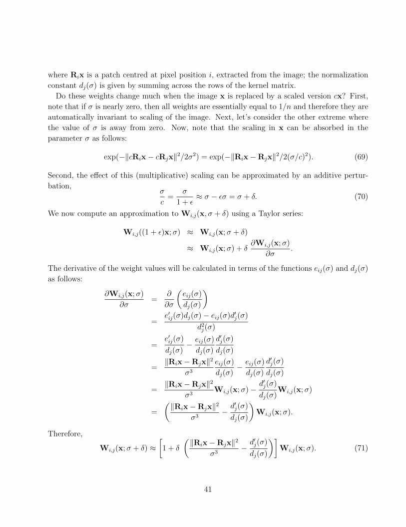
where Rix is a patch centred at pixel position i, extracted from the image; the normalization

constant dj(σ) is given by summing across the rows of the kernel matrix.

Do these weights change much when the image x is replaced by a scaled version cx? First,

note that if σ is nearly zero, then all weights are essentially equal to 1/n and therefore they are

automatically invariant to scaling of the image. Next, let’s consider the other extreme where

the value of σ is away from zero. Now, note that the scaling in x can be absorbed in the

parameter σ as follows:

exp(−‖cRix− cRjx‖2/2σ2) = exp(−‖Rix−Rjx‖2/2(σ/c)2). (69)

Second, the effect of this (multiplicative) scaling can be approximated by an additive pertur-

bation,σ

c=

σ

1 + ε≈ σ − εσ = σ + δ. (70)

We now compute an approximation to Wi,j(x, σ + δ) using a Taylor series:

Wi,j((1 + ε)x;σ) ≈ Wi,j(x;σ + δ)

≈ Wi,j(x;σ) + δ∂Wi,j(x;σ)

∂σ.

The derivative of the weight values will be calculated in terms of the functions eij(σ) and dj(σ)

as follows:

∂Wi,j(x;σ)

∂σ=

∂

∂σ

(eij(σ)

dj(σ)

)=

e′ij(σ)dj(σ)− eij(σ)d′j(σ)

d2j(σ)

=e′ij(σ)

dj(σ)− eij(σ)

dj(σ)

d′j(σ)

dj(σ)

=‖Rix−Rjx‖2

σ3

eij(σ)

dj(σ)− eij(σ)

dj(σ)

d′j(σ)

dj(σ)

=‖Rix−Rjx‖2

σ3Wi,j(x;σ)−

d′j(σ)

dj(σ)Wi,j(x;σ)

=

(‖Rix−Rjx‖2

σ3−d′j(σ)

dj(σ)

)Wi,j(x;σ).

Therefore,

Wi,j(x;σ + δ) ≈[1 + δ

(‖Rix−Rjx‖2

σ3−d′j(σ)

dj(σ)

)]Wi,j(x;σ). (71)

41

Replacing δ = −εσ, we obtain

Wi,j((1 + ε)x;σ) ≈[1− ε

(‖Rix−Rjx‖2

σ2− σ

d′j(σ)

dj(σ)

)]Wi,j(x;σ)

= (1− ε φ(σ)) Wi,j(x;σ).

We can simplify further, but this is not necessary since φ(σ) does not depend on ε. For its part,

φ(σ) behaves like n/σ2. To see this note that the first term in the definition of φ is at worst

n/σ2 since ‖Rix−Rjx‖2 is bounded by n, given that the pixel values are in the range [0, 255].

Similarly, d is on the order of n · exp(‖Rix−Rjx‖2/2σ2), and its derivative d′ is on the order

n · ‖Rix−Rjx‖2 · d/σ3. Consequently, the second term σ · d′/d behaves like ‖Rix−Rjx‖2/σ2

is also on the order n/σ2. Therefore, choosing ε = 1/n, for sufficiently large σ, the term εφ(σ)

becomes negligible.

What we have shown is that the filter weights change very little as a result of the scaling

(1+ε)x as long as ε is very small. Therefore the NLM (and bilateral) filters are (almost exactly)

1-homogeneous as we had hoped.

C.2 Tikhonov Regularizer and Wiener Filtering

We now turn to show that Tikhonov regularization obeys the homogeneity condition. In this

case, the denoised image is the solution of

x = Argminx

1

2σ2‖x− y‖2

2 +λ

2‖Bx‖2

2 , (72)

where B, for example, can be a discrete approximation of a derivative operator. The closed-from

expression of the above minimization is given by

x = f(y) =(I + λσ2BTB

)−1y (73)

= Wy.

When we feed this linear denoiser with the scaled image (1 + ε)y, it gives

f((1 + ε)y) =(I + λσ2BTB

)−1(1 + ε)y, (74)

which is trivially the same as (1 + ε)f(y).

A more challenging case is obtained when the denoiser adapts to the input such that when we

apply f((1+ε)y), the denoiser modifies λ to be λ(1+ε)2. In what follows we return to Equation

(74), but this time with the modified λ, and study the behavior of the filter for infinitesimal

change in ε, i.e.,

limε→0

W(ε) = limε→0

(I + λ(1 + ε)2σ2BTB

)−1. (75)

42

By relying on the first-order Taylor expansion of the above expression and taking the limit

ε→ 0 we get the following

W(ε) ≈ W(0)− ε W(ε)(λ(1 + ε)2σ2BTB

)TW(ε)|ε=0 (76)

= W− ε 2λσ2WBTBW

= (I− ε 2λσ2WBTB)W,

where W = W(0). Therefore, we obtain that the adaptive filter W(ε) changes linearly with

ε. Moreover, ‖σ2WBTB‖ < 1, and thus, if λ� 1 the second term becomes negligible (similar

to what we have shown for the NLM filter). Therefore, we conclude that the image-adaptive

Wiener filtering satisfies the homogeneity condition under mild conditions.

C.3 Patch-Based Denoising

We now turn to discuss state-of-the-art patch-based denoising algorithms. These methods

clean the input noisy image by (i) breaking it into small overlapping patches, (ii) applying a

local denoising step, and (iii) reconstructing the output by averaging the denoised overlapping

patches to form the final image. The wisdom of these algorithms relies on the choice of the local

non-linear prior. Moreover, in most cases, the denoising process can be divided into two parts;

the first contains all the non-linear decisions made by the prior, while the second is nothing

but a linear filter that cleans the noisy patches followed by a patch-averaging step. Clearly, the

latter fulfills the homogeneity condition due to its linearity. In what follows we argue that the

non-linear part of various popular denoisers is stable to an infinitesimal change in scale, thus

leading to an overall satisfaction of the homogeneity property.

Gaussian Mixture Model

We start by the EPLL which can be considered as an iterative GMM denoising algorithm. The

non-linear part of the GMM prior is the choice of a (pre-trained) Gaussian model that best

fits the input noisy patch, and its linear part is the subsequent Wiener filtering step. Consider

a Gaussian model for an n-dimensional patch xi ∼ N(0,Σk), where Σk ∈ Rn×n is the k-th

Gaussian, taken from the mixture. Following the derivations in [43], the MAP estimate is

formulated by

xki = Argminxi

1

2‖xi − yi‖2

2 + σ2xTi Σ−1k xi (77)

=(I + σ2Σ−1

k

)−1yi

= Wki yi,

43

which is nothing but the Wiener filter that cleans the i-th noisy patch yi. The best model for

the i-th patch, k∗i , is the one that maximizing the MAP over all the possible models, given by

k∗i = Argmink‖xki − yi‖2

2 + σ2(xki )TΣ−1

k (xki ) + σ2 log |Σk|. (78)

By plugging Equation (77) into the above we get

k∗i = Argmink‖(Wk

i − I)yi‖22 + σ2(Wk

i yi)TΣ−1

k (Wki yi) + σ2 log |Σk| (79)

= Argmink

Ψ(y, σ,Σk).

When we feed the denoiser with (1 + ε)yi, the above can be written as

k∗,εi = Argmink

(1 + ε)2‖(Wki − I)yi‖2

2 + (1 + ε)2σ2(Wki yi)

TΣ−1k (Wk

i yi) + σ2 log |Σk|(80)

= Argmink‖(Wk

i − I)yi‖22 + σ2(Wk

i yi)TΣ−1

k (Wki yi) +

σ2

(1 + ε)2log |Σk|.

By relying on the relation 1/(1 + ε)2 ≈ 1− 2ε we further simplify the above and obtain

k∗,εi = Argmink‖(Wk

i − I)yi‖22 + σ2(Wk

i yi)TΣ−1

k (Wki yi) + σ2 log |Σk| − 2εσ2 log |Σk|(81)

= Argmink

Ψ(y, σ,Σk)− 2εσ2 log |Σk|.

Now we turn to compare Equation (79) to the one derived above, and get the following condition

on ε that guarantees that k∗,εi = k∗i :

Ψ(y, σ,Σk)− 2εσ2 log |Σk| > Ψ(y, σ,Σk∗)− 2εσ2 log |Σk∗| (82)

Since Ψ(y, σ,Σk) > Ψ(y, σ,Σk∗) one can always choose ε → 0 which will keep this inequality

intact. In an extremely rare case, when Ψ(y, σ,Σk) = Ψ(y, σ,Σk∗), we can modify the GMM

denoiser and propose a simple rule for choosing the model that have a smaller log |Σk| term,

ensuring that k∗,εi = k∗i . To conclude, the non-linear part of the GMM denoising algorithm is

stable to small scaling of the input.

Sparsity-Inspired Denoisers: K-SVD

Given a dictionary, the non-linear mechanism of the K-SVD is the Orthogonal Matching Pursuit

(OMP) [62] algorithm, which estimates the sparse representation of an input noisy patch. This

is a greedy method, aiming to approximate the solution of

αi = Argminαi‖αi‖0 s.t. ‖yi −Dαi‖2

2 ≤ nσ2, (83)

44

where n is the size of the patch, and D ∈ Rn×m is a (possibly redundant, m > n, and non-

orthogonal) dictionary. At each step, denoted by k, the OMP picks a new atom (a column

from D) that minimizes the residual. Formally, the rule for choosing the first atom dj1 can be

written as

j1 = Argmaxj|dTj yi|, (84)

while in the t-th step of the OMP, it is the one that maximizing

jt = Argmaxj|dTj rti|, (85)

where rti = yi −DStiαti is the residual. We denoted by Sti the set of chosen atoms, obtained in

the previous steps, and by DSti∈ Rn×|Sti | the corresponding dictionary – a matrix having the

chosen atoms as its columns. This expression can be further simplified by relying on the fact

that the representation is the outcome of a least-squares solution, given by

αti =(DTSti

DSti

)−1

DTSti

yi. (86)

Substituting the above in Equation (85) results in

jt = Argmaxj|dTj ri| = Argmax

j

∣∣∣∣dTj (I−(DTSti

DSti

)−1

DTSti

)yi

∣∣∣∣ . (87)

This process is repeated until reaching to the error constraint.

Trivially, scaling the input patch would not modify the result of Equations (84) and (87).

However, scaling the input may modify the stopping rule, and thereby the number of atoms

that the OMP picks. This will happen only when ‖yi −Dαi‖22 = nσ2, which is an extremely

rare case. Notice that given the final set of chosen atoms, S∗i , the cleaned patch is given by

xi = DS∗i

(DTS∗i

DS∗i

)−1

DTS∗i

yi, which clearly satisfies the homogeneity condition. To conclude,

we showed that the non-linear part of the OMP is stable to an infinitesimal change in scale, and

since the cleaned patch is simply obtained by a linear projection onto the chosen atoms we have

that with high probability the OMP (and thus the K-SVD) fulfills our hope for homogeneity.

D The Differentiability Requirement

In the opening of Section 3.1, we required the denoising engine f(x) to be differentiable. Why?

There are several benefits for having this behavior:

1. The directional derivative property, ∇xf(x)x = f(x), which emerges from the homogene-

ity condition, becomes possible.

45

2. The passivity condition, which refers to the spectral radius of ∇xf(x), stands on solid

grounds.

3. The convergence of the fixed-point algorithm discussed in Section 4.2 is guaranteed.

4. The convexity of the regularization term ρL(x), discussed in Section 5.1, and emerging

from Condition 2, becomes possible.

All these are good reasons for demanding differentiability of the denoiser f(x), and yet, the

question is whether it is too limiting or whether this requirement could be circumvented.

Observe that Point 1 above could rely on the availability of a far weaker requirement of the

availability of all directional derivatives of the form ∇xf(x)x. Indeed, the passivity mentioned

in Point 2 could also be posed in terms of a directional derivative, replacing Equation (15) by

the somewhat weaker requirement

∀x 6= 0,xT∇xf(x)x

xTx≤ 1,

under the assumption that ∇xf(x) is symmetric.

The question we leave as open at this stage is whether Points 3 and 4 above (convergence

of the FP algorithm and the convexity of our regularization) could rely on the existence of all

directional derivatives. At worst, if indeed the denoising engine is not differentiable but has all

its directional derivatives, Points 3 and 4 are lost, and the behavior of the proposed algorithm

is not clear from a theoretical standpoint.

A different, and more practical question is whether differentiability assumption on f(x) is

feasible in existing algorithms. The NLM and the Bilateral filter are clearly differentiable.

TNRD is differentiable as well since its non-linearities are smooth (linear combination of Gaus-

sian RBF’s). EPLL, BM3D, are K-SVD more challenging since their non-linear parts include

sharp-decisions. Each of these methods could be ε-modified to have a fuzzy decision, thus

rendering all of them differentiable with hardly any change in their actual behavior.

References

[1] A. Buades, B. Coll, and J.M. Morel, A Non-Local Algorithm for Image Denoising, CVPR,

2005.

[2] C. Kervrann and J. Boulanger, Optimal Spatial Adaptation for Patch-Based Image De-

noising, IEEE Trans. on Image Processing, Vol. 15, No. 10, pp. 2866–2878, October 2006.

[3] T. Tasdizen, Principal Neighborhood Dictionaries for Nonlocal Means Image Denoising,

IEEE Trans. on Image Processing, Vol. 18, No. 12, pp. 2649–2660, 2009.

46

[4] M. Elad and M. Aharon, Image Denoising via Sparse and Redundant Representations Over

Learned Dictionaries, IEEE Trans. on Image Processing, Vol. 15, No. 12, pp. 3736–3745,

2006.

[5] K. Dabov, A. Foi, V. Katkovnik, and K. Egiazarian, Image Denoising by Sparse 3-D

Transform-Domain Collaborative Filtering, IEEE Trans. on Image Processing, Vol. 16,

No. 8, pp. 2080–2095, 2007.

[6] H. Takeda, S. Farsiu, and P. Milanfar, Kernel Regression for Image Processing and Recon-

struction, IEEE Trans. on image processing, Vol. 16, No. 2, 349–366, 2007.

[7] J. Mairal, F. Bach, J. Ponce, G. Sapiro, and A. Zisserman, Non-Local Sparse Models for

Image Restoration, ICCV, 2009.

[8] W. Dong, X. Li, L. Zhang, and G. Shi, Sparsity-Based Image Denoising via Dictionary

Learning and Structural Clustering, CVPR, 2011.

[9] W. Dong, L. Zhang, G. Shi, and X. Li, Nonlocally Centralized Sparse Representation for

Image Restoration, IEEE Trans. on Image Processing, Vol. 22, No. 4, pp. 1620–1630, 2013.

[10] P. Chatterjee and P. Milanfar, Patch-Based Near-Optimal Image Denoising, IEEE Trans.

on Image Processing, Vol. 21, No. 4, pp. 1635–1649, 2012.

[11] H.C. Burger, C.J. Schuler, and S. Harmeling, Image denoising: Can Plain Neural Networks

Compete With BM3D?, CVPR, 2012.

[12] M. Lebrun, M. Colom, A. Buades, and J.-M. Morel, Secrets of Image Denoising Cuisine,

Acta Numerica, Vol. 21, No. 4, pp. 475–576, 2012.

[13] M. Lebrun, A. Buades, and J.-M. Morel, Implementation of the “Non- Local Bayes” (NL-

Bayes) Image Denoising Algorithm, IPOL, Vol. 3, pp, 1–42, 2013.

[14] C. Knaus and M. Zwicker, Dual-Domain Image Denoising, ICIP, 2013.

[15] H. Talebi and P. Milanfar, Global image denoising, IEEE Transactions on Image Process-

ing, Vol. 23, No. 2, pp. 755–768, 2014.

[16] S. Gu, L. Zhang, W. Zuo, and X.Feng, Weighted Nuclear Norm Minimization with Appli-

cation to Image Denoising, CVPR, 2014.

[17] W. Dong, G. Shi, Y. Ma, and X. Li, Image Restoration via Simultaneous Sparse Coding:

Where Structured Sparsity Meets Gaussian Scale Mixture, Int. Journal of Computer Vision

(IJCV), Vol. 114, No. 2, pp. 217–232, 2015.

47

[18] N. Pierazzo, M. Rais, J.-M. Morel, and G. Facciolo, DA3D: Fast and Data Adaptive Dual

Domain Denoising, ICIP, 2015.

[19] P. Milanfar, Symmetrizing Smoothing Filters, SIAM Journal on Imaging Science, Vol. 6,

No. 1, pp. 263284, 2013.

[20] Y. Chen and T. Pock, Trainable Nonlinear Reaction Diffusion: A Flexible Framework for

Fast and Effective Image Restoration, arXiv, 1508.02848, 2015.

[21] P. Chatterjee and P. Milanfar, Is Denoising Dead? IEEE Trans. on Image Processing, Vol.

19, No. 4, pp. 895–911, 2010.

[22] A. Levin and B. Nadler, Natural Image Denoising: Optimality and Inherent Bounds,

CVPR, 2011.

[23] A. Levin, B. Nadler, F. Durand, and W.T. Freeman, Patch Complexity, Finite Pixel Cor-

relations and Optimal Denoising, ECCV, 2012.

[24] M. Protter, M. Elad, H. Takeda, and P. Milanfar, Generalizing the Nonlocal-Means to

Superresolution Reconstruction, IEEE Trans. Image Processing, Vol. 18, No. 1, pp. 36–51,

2009.

[25] S. Ravishankar and Y. Bresler, MR Image Reconstruction From Highly Undersampled k-

Space Data by Dictionary Learning, IEEE Trans. on Medical Imaging, Vol. 30, No. 5, pp.

1028–1041, 2011.

[26] M. Akcakaya, T.A. Basha, B. Goddu, L.A. Goepfert, K.V. Kissinger, V. Tarokh, W.J.

Manning, and R. Nezafat, Low-Dimensional Structure Self-Learning and Thresholding:

Regularization Beyond Compressed Sensing for MRI Reconstruction, Magnetic Resonance

in Medicine, Vol. 66, No. 3, pp. 756–767, 2011.

[27] A. Danielyan, V. Katkovnik, and K. Egiazarian, BM3D Frames and Variational Image

Deblurring, IEEE Trans. on Image Processing, Vol. 21, No. 4, pp. 1715–1728, 2012.

[28] W. Dong, L. Zhang, R. Lukac, and G. Shi, Sparse Representation based Image Interpola-

tion with Nonlocal Autoregressive Modeling, IEEE Trans. on Image Processing, Vol. 22,

No. 4, pp. 1382–1394, 2013.

[29] C.A. Metzler, A. Maleki, and R.G. Baraniuk, Optimal Recovery From Compressive Mea-

surements via Denoising-Based Approximate Message Passing, SAMPTA, 2015.

[30] S.V. Venkatakrishnan, C.A. Bouman, and B. Wohlberg, Plug-and-Play Priors for Model

Based Reconstruction, GlobalSIP, 2013.

48

[31] S.H. Chan, Algorithm-Induced Prior for Image Restoration, ArXiv, 1602.00715, 2016.

[32] S.H. Chan, X. Wang, and O.A. Elgendy, Plug-and-Play ADMM for Image Restoration:

Fixed Point Convergence and Applications, ArXiv, 1605.01710, 2016.

[33] S. Sreehari, S.V. Venkatakrishnan, B. Wohlberg, L.F. Drummy, J.P. Simmons, and C.A.

Bouman, Plug-and-Play Priors for Bright Field Electron Tomography and Sparse Interpo-

lation, ArXiv, 1512.07331, 2015.

[34] Y. Dar, A.M. Bruckstein, M. Elad, and R. Giryes, Postprocessing of Compressed Images

via Sequential Denoising, IEEE Trans. on Image Processing, Vol. 25, No. 7, pp. 3044 -

3058, 2016.

[35] M.U. Sadiq , J.P. Simmons, and C.A. Bouman, Model Based Image Reconstruction with

Physics Based Priors, ICIP, 2016.

[36] A.M. Teodoro, J.M. Bioucas-Dias, and M.A.T. Figueiredo, Image Restoration with Locally

Selected Class-Adapted Models, ICIP, 2016.

[37] A. Brifman, Y. Romano, and M. Elad, Turning a Denoiser into a Super-Resolver Using

Plug and Play Priors, ICIP, 2016.

[38] A.M. Teodoro, J.M. Bioucas-Dias, and M.A.T. Figueiredo, Hyperspectral Sharpening Us-

ing Scene-Adapted Gaussian Mixture Priors, ArXiv, 1702.02445, February 2017.

[39] R.L. Lagendijk and J. Biemond, Iterative Identification and Restoration of Images,

Springer, 1990.

[40] L. I. Rudin, S. Osher, and E. Fatemi, Nonlinear total variation based noise removal algo-

rithms, Phys. D, vol. 60, no. 1-4, pp. 259268, Nov. 1992.

[41] S Mallat, A Wavelet Tour of Signal Processing, Academic Press, 1999.

[42] D. Zoran and Y. Weiss, From Learning Models of Natural Image Patches to Whole Image

Restoration, CVPR 2011.

[43] G. Yu, G. Sapiro, and S. Mallat, Solving Inverse Problems with Piecewise Linear Es-

timators: From Gaussian Mixture Models to Structured Sparsity, IEEE Trans. Image

Processing, Vol. 21, No. 5, pp. 2481–2499, 2012.

[44] A.M. Bruckstein, D.L. Donoho, and M. Elad, From Sparse Solutions of Systems of Equa-

tions to Sparse Modeling of Signals and Images, SIAM Review, Vol. 51, No. 1, pp. 34–81,

2009.

49

[45] A. Vedaldi and A. Zisserman, Efficient Additive Kernels via Explicit Feature Maps, IEEE

Trans Pattern Anal Mach Intell. 2012 Mar vo. 34, no. 3, pp. 480-92

[46] X. Glorot, A. Bordes, and Y. Bengio, Deep sparse rectifier neural networks, in Aistats,

vol. 15, p. 275, 2011.

[47] V. Papyan, Y. Romano, and M. Elad, Convolutional Neural Networks Analyzed via Con-

volutional Sparse Coding, ArXiv, 1607.08194, October 2016.

[48] A. Elmoataz, O. Lezoray, and S. Bougleux, Nonlocal Discrete Regularization on Weighted

Graphs: A Framework for Image and Manifold Processing, IEEE Trans. Image Processing,

Vol. 17, No. 7, pp. 1047–1060, 2008.

[49] A.D. Szlam, M. Maggioni, and R.R. Coifman, Regularization on Graphs with Function-

Adapted Diffusion Processes, Journal on Machine Learning Research, Vol. 9, pp. 1711–

1739, 2008.

[50] S. Bougleux, A. Elmoataz, and M. Melkemi, Local and Nonlocal Discrete Regularization

on Weighted Graphs for Image and Mesh Processing, Int. Journal on Computer Vision,

Vol. 84, pp. 220–236, 2009.

[51] G. Peyre, S. Bougleux, and L.D. Cohen, Non-local Regularization of Inverse Problems,

Inverse Problems and Imaging, Vol. 5, No. 2, pp. 511–530, 2011.

[52] P. Milanfar, A Tour of Modern Image Filtering: New Insights and Methods, both Practical

and Theoretical, IEEE Signal Processing Magazine, Vol. 30, No. 1, pp. 106–128, 2013.

[53] F.G. Meyer and X. Shen, Perturbation of the Eigenvectors of the Graph Laplacian: Ap-

plication to Image Denoising, Applied Computational Harmonic Analysis, Vol. 36, No. 2,

pp. 326–334, 2014.

[54] X. Liu, D. Zhai, D. Zhao, G. Zhai, and W. Gao, Progressive Image Denoising Through

Hybrid Graph Laplacian Regularization: A Unified Framework, IEEE Trans. Image Pro-

cessing, Vol. 23, No. 4, pp. 1491–1503, 2014.

[55] S.M. Haque, G. Pai, and V.M. Govindu, Symmetric Smoothing Filters From Global Con-

sistency Constraints, IEEE Trans. Image Processing, Vol. 24, No. 5, pp. 1536–1548, 2014.

[56] A. Kheradmand and P. Milanfar, A General Framework for Regularized, Similarity-Based

Image Restoration, IEEE Trans. Image Processing, Vol. 23, No. 12, pp. 5136–5151, 2014.

[57] Y. Romano and M. Elad, Boosting of Image Denoising Algorithms, SIAM Journal on

Imaging Sciences, Vol. 8, No. 2, pp. 1187–1219, June 2015.

50

[58] S. Boyd, N. Parikh, E. Chu, B. Peleato, and J. Eckstein, Distributed Optimization and

Statistical Learning via the Alternating Direction Method of Multipliers, Foundations and

Trends in Machine Learning, Vol. 3, No. 1, pp. 1–122, July 2011.

[59] M. Afonso, J. Bioucas-Dias, and M.A.T. Figueiredo, Fast Image Recovery Using Variable

Splitting and Constrained Optimization, IEEE Trans. on Image Processing, Vol. 19, No.

9, pp. 2345–2356, 2010.

[60] M. Afonso, J. Bioucas-Dias, and M.A.T. Figueiredo, An Augmented Lagrangian Approach

to the Constrained Optimization Formulation of Imaging Inverse Problems, IEEE Trans

on Image Processing, Vol. 20, No. 3, pp. 681–695, 2011.

[61] N. Parikh and S. Boyd, Proximal Algorithms, Foundations and Trends in Optimization,

Vol. 1, No. 3, pp. 123–231, 2014.

[62] Y. C. Pati, R. Rezaiifar, and P. S. Krishnaprasad, Orthogonal Matching Pursuit: Recursive

Function Approximation with Applications to Wavelet Decomposition, IEEE Asilomar

Conf. Signals, Syst. Comput., pp. 40–44, 1993.

[63] E. Candes and T. Tao, The Dantzig Selector: Statistical Estimation When p is Much

Larger than n, Annals of Statistics, Vol. 35, No. 6, pp. 2313–2351, 2007.

[64] Y. Romano and M. Elad, Improving K-SVD Denoising by Post-Processing its Method-

Noise, ICIP, 2013.

[65] H. Talebi, X. Zhu, and P. Milanfar, How to SAIF-ly Boost Denoising Performance, IEEE

Trans. on Image Processing, Vol. 22, No. 4, pp. 1470–1485, 2013.

[66] T.M. Apostol, Calculus, 2-nd Edition, Volume 1, Waltham, Massachusetts – Blaisdell,

1967.

[67] S. Boyd and L. Vandenberghe, Convex Optimization, Cambridge University Press, 2004.

[68] M. Elad, Sparse and Redundant Representations: From Theory to Applications in Signal

and Image Processing, Springer, 1st Edition, 2010.

[69] G.H. Golub and C.F. Van Loan, Matrix Computations, John Hopkins University Press,

3-rd Edition, Baltimore, 1996.

[70] M. Elad, B. Matalon, and M. Zibulevsky, Coordinate and Subspace Optimization Methods

for Linear Least Squares with Non-Quadratic Regularization, Applied and Computational

Harmonic Analysis, Vol. 23, No. 3, pp. 346–367, 2007.

51

[71] M. Droske and A. Bertozzi, Higher-Order Feature-Preserving Geometric Regularization,

SIAM Journal on Imaging Sciences, Vol. 3, No. 1, pp. 21–51, 2010.

[72] A. Beck and M. Teboulle, Fast Gradient-Based Algorithms for Constrained Total Variation

Image Denoising and Deblurring Problems, IEEE Transactions on Image Processing, Vol.

18, No. 11, pp. 2419–2434, 2009.

[73] W. Dong, L. Zhang, G. Shi, and X. Wu, Image Deblurring and Super-Resolution by Adap-

tive Sparse Domain Selection and Adaptive Regularization, IEEE Transactions on Image

Processing, Vol. 20, No. 7, pp. 1838–1857, 2011.

52