the little engine that could: regularization by denoising (red) - … · 2018-06-03 · key words....
TRANSCRIPT
Copyright © by SIAM. Unauthorized reproduction of this article is prohibited.
SIAM J. IMAGING SCIENCES c© 2017 Society for Industrial and Applied MathematicsVol. 10, No. 4, pp. 1804–1844
The Little Engine That Could:Regularization by Denoising (RED)∗
Yaniv Romano† , Michael Elad‡ , and Peyman Milanfar‡
Abstract. Removal of noise from an image is an extensively studied problem in image processing. Indeed, therecent advent of sophisticated and highly effective denoising algorithms has led some to believe thatexisting methods are touching the ceiling in terms of noise removal performance. Can we leveragethis impressive achievement to treat other tasks in image processing? Recent work has answered thisquestion positively, in the form of the Plug-and-Play Prior (P 3) method, showing that any inverseproblem can be handled by sequentially applying image denoising steps. This relies heavily on theADMM optimization technique in order to obtain this chained denoising interpretation. Is this theonly way in which tasks in image processing can exploit the image denoising engine? In this paperwe provide an alternative, more powerful, and more flexible framework for achieving the same goal.As opposed to the P 3 method, we offer Regularization by Denoising (RED): using the denoisingengine in defining the regularization of the inverse problem. We propose an explicit image-adaptiveLaplacian-based regularization functional, making the overall objective functional clearer and betterdefined. With a complete flexibility to choose the iterative optimization procedure for minimizingthe above functional, RED is capable of incorporating any image denoising algorithm, can treatgeneral inverse problems very effectively, and is guaranteed to converge to the globally optimalresult. We test this approach and demonstrate state-of-the-art results in the image deblurring andsuper-resolution problems.
Key words. image denoising engine, Plug-and-Play Prior, Laplacian regularization, inverse problems
AMS subject classifications. 62H35, 68U10, 94A08
DOI. 10.1137/16M1102884
1. Introduction. We open this paper with a bold and possibly controversial statement:To a large extent, removal of zero-mean white additive Gaussian noise from an image is asolved problem in image processing.
Before justifying this statement, let us describe the basic building block that will be thestar of this paper: the image denoising engine. From the humble linear Gaussian filter tothe recently developed state-of-the-art methods using convolutional neural networks, there isno shortage of denoising approaches. In fact, these algorithms are so widely varied in theirdefinition and underlying structure that a concise description will need to be made carefully.Our story begins with an image x corrupted by zero-mean white additive Gaussian noise,
(1) y = x + e.
∗Received by the editors November 9, 2016; accepted for publication (in revised form) August 29, 2017; publishedelectronically October 19, 2017.
http://www.siam.org/journals/siims/10-4/M110288.htmlFunding: The first author’s research was supported by European Research Council grant 320640.†The Electrical Engineering Department, The Technion - Israel Institute of Technology, Haifa, 32000, Israel
([email protected]).‡Google Research, Mountain View, CA 94043 ([email protected], [email protected]).
1804
Dow
nloa
ded
10/1
9/17
to 3
8.98
.219
.157
. Red
istr
ibut
ion
subj
ect t
o SI
AM
lice
nse
or c
opyr
ight
; see
http
://w
ww
.sia
m.o
rg/jo
urna
ls/o
jsa.
php

Copyright © by SIAM. Unauthorized reproduction of this article is prohibited.
REGULARIZATION BY DENOISING (RED) 1805
In our notation, we consider an image as a vector of length n (after lexicographic ordering).In the above description, the noise vector is normally distributed: e ∼ N
(0, σ2I
). In the most
general terms, the image denoising engine is a function f : [0, 255]n −→ [0, 255]n that mapsan image y to another image of the same size x = f(y), with the hope of getting as closeas possible to the original image x. Ideally, such functions operate on the input image y toremove the deleterious effect of the noise while maintaining edges and textures beneath.
The claim made above about the denoising problem being solved is based on the availabilityof algorithms proposed in the past decade that can treat this task extremely effectively andstably, getting very impressive results, which also tend to be quite concentrated (see, forexample, the work reported in [3, 4, 5, 6, 7, 8, 9, 10, 11, 12, 13, 14, 15, 16, 17, 18, 42]). Indeed,these documented results have led researchers to the educated guess that these methods aregetting very close to the optimally possible denoising performance [21, 22, 23]. This alignswell with the unspoken observation in our community in recent years that investing more workto improve image denoising algorithms seems to lead to diminishing returns.
While the above may suggest that work on denoising algorithms is turning to a dead-endavenue, a new opportunity emerges from this trend: seeking ways to leverage the vast progressmade on the image denoising front in order to treat other tasks in image processing, bringingtheir solutions to new heights. One natural path towards addressing this goal is to take anexisting and well-performing denoising algorithm and generalize it to handle a new problem.This has been the logical path that has led to contributions such as [24, 25, 26, 27, 28, 29]and many others. These papers, and others like them, offer an exhaustive manual adaptationof existing denoising algorithms, carefully retailored to handle specific alternative problems.This line of work, while often successful, is quite limited, as it offers no flexibility and nogeneral scheme for diverting image denoising engines to treat new image processing tasks.
Could one offer a more systematic way to exploit the abundance of high-performing im-age denoising algorithms to treat a much broader family of problems? The recent work byVenkatakrishnan, Bouman, and Wohlberg provides a positive and tantalizing answer to thisquestion, in the form of the Plug-and-Play Prior (P 3) method [30, 31, 32, 33]. This tech-nique builds on the use of an implicit prior for regularizing general inverse problems. Whenhandling the obtained optimization task via the ADMM optimization scheme [57, 58, 59], theoverall problem decomposes into a sequence of image denoising tasks, coupled with simplerL2-regularized inverse problems that are much easier to handle.
While the P 3 scheme may sound like the perfect answer to our prayers, reality is somewhatmore complicated. First, this method is not always accompanied by a clear definition of theobjective function, since the regularization being effectively used is only implicit, implied bythe denoising algorithm. Indeed, it is not clear at all that there is an underlying objectivefunction behind the P 3 scheme if arbitrary denoising engines are used [31]. Second, parametertuning of the ADMM scheme is a delicate matter, and especially so under a nonprovableconvergence regime, as is the case when using sophisticated denoising algorithms. Third,being intimately coupled with the ADMM, the P 3 scheme does not offer easy and flexibleways of replacing the iterative procedure. Because of these reasons, the P 3 scheme is neithera turn-key tool, nor is it free from emotional involvement. Nevertheless, the P 3 method hasdrawn much attention (see, e.g., [31, 32, 33, 34, 35, 36, 37, 38]), and rightfully so, as it offers aclear path towards harnessing a given image denoising engine for treating more general inverseD
ownl
oade
d 10
/19/
17 to
38.
98.2
19.1
57. R
edis
trib
utio
n su
bjec
t to
SIA
M li
cens
e or
cop
yrig
ht; s
ee h
ttp://
ww
w.s
iam
.org
/jour
nals
/ojs
a.ph
p
Copyright © by SIAM. Unauthorized reproduction of this article is prohibited.
1806 YANIV ROMANO, MICHAEL ELAD, AND PEYMAN MILANFAR
problems, just as described above.Is there a more general alternative to the P 3 method that could be simpler and more
stable? This paper puts forward such a framework, offering a systematic use of such denoisingengines for regularization of inverse problems. We term the proposed method Regularizationby Denoising (RED), relying on a general structured smoothness penalty term harnessed toregularize any desired inverse problem. More specifically, the regularization term we proposein this work is the following:
(2) ρ(x) =12
xT [x− f(x)] ,
in which the denoising engine itself is applied on the candidate image x, and the penaltyinduced is proportional to the inner product between this image and its denoising residual.This defined smoothness regularization is effectively using an image-adaptive Laplacian, whichin turn draws its definition from the arbitrary image denoising engine of choice, f(·). Sur-prisingly, under mild assumptions on f(·), it is shown that the gradient of the regularizationterm is manageable, given as the denoising residual, x − f(x). Therefore, armed with thisregularization expression, we show that any inverse problem can be handled while calling thedenoising engine iteratively.
RED, the newly proposed framework, is much more flexible in the choice of the optimiza-tion method to use, not being tightly coupled to one specific technique, as in the case of theP 3 scheme (relying on ADMM). Another key difference w.r.t. the P 3 method is that ouradaptive Laplacian-based regularization functional is explicit, making the overall Bayesianobjective function clearer and better defined. RED is capable of incorporating any imagedenoising algorithm, and can treat general inverse problems very effectively, while resultingin an overall algorithm with very simple structure.
An important advantage of RED over the P 3 scheme is the flexibility with which one canchoose the denoising engine f(·) to plug in the regularization term. While most of the discus-sion in this paper keeps focusing on white Gaussian noise (WGN) removal, RED can actuallydeploy almost any denoising engine. Indeed, we define a set of two mild conditions that f(·)should satisfy and show that many known denoising methods obey these properties. As an ex-ample, in our experiments we show how the median filter can become an effective regularizer.Last but not least, we show that the defined regularization term is a convex function, implyingthat in most cases, in which the log-likelihood term is convex too, the proposed algorithms areguaranteed to converge to a global optimum solution. We demonstrate this scheme, showingstate-of-the-art results in image deblurring and single image super-resolution.
This paper is organized as follows: In the next section we present the background materialfor this work, discussing the general form of inverse problems as optimization tasks, andpresenting the P 3 scheme. Section 3 focuses on the image denoising engine, defining it andits properties clearly, so as to enable its use in the proposed Laplacian paradigm. Section 4serves the main part of this work—introducing RED: a new way to use an image denoisingengine to handle general structured inverse problems. In section 5 we analyze the proposedscheme, discussing convexity, an alternative formulation, and a qualitative comparison to theP 3 scheme. Results on the image deblurring and single-image super-resolution problems arebrought in section 6, demonstrating the strength of the proposed scheme. We conclude theD
ownl
oade
d 10
/19/
17 to
38.
98.2
19.1
57. R
edis
trib
utio
n su
bjec
t to
SIA
M li
cens
e or
cop
yrig
ht; s
ee h
ttp://
ww
w.s
iam
.org
/jour
nals
/ojs
a.ph
p

Copyright © by SIAM. Unauthorized reproduction of this article is prohibited.
REGULARIZATION BY DENOISING (RED) 1807
paper in section 7 with a summary of the open questions that we identify for future work.
2. Preliminaries. In this section we provide background material that serves as the foun-dation to this work. We start by presenting the breed of optimization tasks we will work onthroughout the paper for handling the inverse problems of interest. We then introduce theP 3 method and discuss its merits and weaknesses.
2.1. Inverse problems as optimization tasks. Bayesian estimation of an unknown imagex given its measured version y uses the posterior conditional probability, P (x|y), in orderto infer x. The most popular estimator in this regime is the maximum a posteriori proba-bility (MAP), which chooses the mode (x for which the maximum probability is obtained)of the posterior. Using Bayes’s rule, this implies that the estimation task is turned into anoptimization problem of the form
xMAP = Argmaxx
P (x|y) = Argmaxx
P (y|x)P (x)P (y)
= Argmaxx
P (y|x)P (x)(3)
= Argminx− log{P (y|x)} − log{P (x)}.
In the above derivations we exploited the fact that P (y) is not a function of x, and thus it canbe omitted. We also used the fact that the − log function is monotonic decreasing, turningthe maximization into a minimization problem.
The term − log{P (y|x)} is known as the log-likelihood term, and it encapsulates theprobabilistic relationship between the desired image x and the measurements y, under theassumption that the desired image is known. We shall rewrite this term as
`(y,x) = − log{P (y|x)}.(4)
As a classic example for the log-likelihood that will accompany us throughout this paper, theexpression `(y,x) = 1
2σ2 ‖Hx − y‖22 refers to the case of y = Hx + e, where H is a lineardegradation operator and e is WGN contamination of variance σ2. Naturally, if the noisedistribution changes, we depart from the comfortable L2 form.
The second term in (3), − log{P (x)}, refers to the prior, bringing in the influence of thestatistical nature of the unknown. This term is also referred to as the regularization, as ithelps in better conditioning the overall optimization task in cases where the likelihood alonecannot lead to a unique or stable solution. We shall rewrite this term as
λρ(x) = − log{P (x)},(5)
where λ is a scalar that encapsulates the confidence in this term.What is ρ(x) and how is it chosen? This is the holy grail of image processing, with a
progressive advancement over the years of better modeling the image statistics and leveragingthis for handling various tasks in image processing. Indeed, one could claim that almosteverything done in our field surrounds this quest for choosing a proper prior, from the earlysmoothness prior ρ(x) = λxTLx using the classic Laplacian [39], through total variation [40]and wavelet sparsity [41], all the way to recent proposals based on patch-based GMM [42, 43]and sparse-representation modeling [44]. Interestingly, the work we report here builds on theD
ownl
oade
d 10
/19/
17 to
38.
98.2
19.1
57. R
edis
trib
utio
n su
bjec
t to
SIA
M li
cens
e or
cop
yrig
ht; s
ee h
ttp://
ww
w.s
iam
.org
/jour
nals
/ojs
a.ph
p

Copyright © by SIAM. Unauthorized reproduction of this article is prohibited.
1808 YANIV ROMANO, MICHAEL ELAD, AND PEYMAN MILANFAR
surprising comeback of the Laplacian regularization in a much more sophisticated form, asreported in [47, 48, 49, 50, 51, 52, 53, 54, 55, 56].
Armed with a clear definition of the relation between the measurements and the unknown,and with a trusted prior, the MAP estimation boils down to the optimization problem of theform
xMAP = Argminx
`(y,x) + λρ(x).(6)
This defines a wide family of inverse problems that we aim to address in this work, which in-cludes tasks such as denoising, deblurring, super-resolution, demosaicing, tomographic recon-struction, optical-flow estimation, segmentation, and many other problems. The randomnessin these problems is typically due to noise contamination of the measurements, and this couldbe Gaussian, Laplacian, Gamma-distributed, Poisson, and other noise models.
2.2. The Plug-and-Play Prior (P 3) approach. For completeness of this exposition, webriefly review the P 3 approach. Aiming to solve the problem posed in (6), the ADMMtechnique [57, 58, 59] suggests handling this by variable splitting, leading to the equivalentproblem
{xMAP , v} = Argminx,v
`(y,x) + λρ(v) s.t. x = v.(7)
The constraint is turned into a penalty term, relying on the augmented Lagrangian method(in its scaled dual form [57]), leading to
{xMAP , v} = Argminx,v
`(y,x) + λρ(v) +β
2‖x− v + u‖22,(8)
where u serves as the Lagrange multiplier vector for the set of constraints. ADMM addressesthe resulting problem by updating x, v, and u sequentially in a block-coordinate-descentfashion, leading to the following series of subproblems:
1. Update of x: When considering v (and u) as fixed, the term ρ(v) is omitted, andour task becomes
x = Argminx
`(y,x) +β
2‖x− v + u‖22,(9)
which is a far simpler inverse problem, where the regularization is an L2 proximityone, which is easy to solve in most cases.
2. Update of v: In this stage we freeze x (and u), and thus the log-likelihood termdrops, leading to
v = Argminv
λρ(v) +β
2‖x− v + u‖22.(10)
This stage is nothing but a denoising of the image x + u, assumed to be contaminatedby a white additive Gaussian noise of power σ2 = 1/β. This is easily verified byreturning to (6) and plugging the log-likelihood term ‖v − x − u‖22/2σ2 referring tothis case. Indeed, this is the prime observation in [30], as the authors suggest replacingD
ownl
oade
d 10
/19/
17 to
38.
98.2
19.1
57. R
edis
trib
utio
n su
bjec
t to
SIA
M li
cens
e or
cop
yrig
ht; s
ee h
ttp://
ww
w.s
iam
.org
/jour
nals
/ojs
a.ph
p

Copyright © by SIAM. Unauthorized reproduction of this article is prohibited.
REGULARIZATION BY DENOISING (RED) 1809
the direct solution of (10) by activating an image denoising engine of choice. This way,we do not need to define explicitly the regularization ρ(·) to be used, as it is impliedby the engine chosen.
3. Update of u: We complete the algorithm description by considering the update ofthe Lagrange multiplier vector u, which is done by u = u + x− v.
Although the above algorithm has a clear mathematical formulation and only two parameters,denoted by β and λ, it turns out that tuning these is not a trivial task. The source ofcomplexity emerges from the fact that the input noise level to the denoiser is equal to
√λ/β.
The confidence in the prior is determined by λ, and the penalty on the distance between x andv is affected by β. Empirically, setting a fixed value of β does not seize the potential of thisalgorithm; following previous work (see, e.g. [32, 37]), a common practical strategy to achievea high-quality estimation is to increase the value of β as a function of the iterations: startingfrom a relatively small value, i.e., allowing an aggressive regularization, then proceeding toa more conservative one that limits the smoothing effect, up to a point where β should belarge enough to ensure convergence [32] and to avoid an undesired oversmoothed outcome.As one can imagine, it is cumbersome to choose the rate in which β should be increased,especially because the corrupted image x + u is a function of the Lagrange multiplier, whichvaries through the iterations as well.
In terms of convergence, the P 3 scheme has been shown to be well-behaved under someconditions on the denoising algorithm used. While the work reported in [31] requires thedenoiser to be a symmetric smoothing and nonexpansive filter, the later work in [32] relaxesthis condition to much simpler boundedness of the denoising effect. However, both of theseprove at best a convergence to a steady-state outcome, which is very far from the desiredclaim of getting to the global minimizer of the overall objective function. The work reportedin [33] offers clear conditions for a global convergence of P 3, requiring the denoiser to benonexpansive, and emerging as the minimizer of a convex functional. A recently releasedpaper extends the above by using a specific GMM-based denoiser, showing that these twoconditions are met, thus guaranteeing global convergence of their ADMM scheme [38].
Indeed, in that respect, a delicate matter with the P 3 approach is the fact that given achoice of a denoising engine, it does not necessarily refer to a specific choice of a prior ρ(·), asnot every such engine could have a MAP-oriented interpretation. This implies a fundamentaldifficulty in the P 3 scheme, as in this case we will be activating a denoising algorithm whiledeparting from the original setting we have defined, and having no underlying cost functionto serve. Indeed, the work reported in [31] addresses this very matter in a narrower setting,by studying the identity of the effective prior obtained from a chosen denoising engine. Theauthor chooses to limit the answer to symmetric smoothing filters, showing that even in thisspecial case, the outcome is far from being trivial. As we are about to see in the next section,this shortcoming can be overcome by adopting a different regularization strategy.
3. The image denoising engine. Image denoising is a special case of the inverse problemposed in (6), referring to the case y = x + e, where e is WGN contamination of variance σ2.In this case, the MAP problem becomes
xDenoise = Argminx
12σ2 ‖y− x‖22 + λρ(x).(11)
Dow
nloa
ded
10/1
9/17
to 3
8.98
.219
.157
. Red
istr
ibut
ion
subj
ect t
o SI
AM
lice
nse
or c
opyr
ight
; see
http
://w
ww
.sia
m.o
rg/jo
urna
ls/o
jsa.
php
Copyright © by SIAM. Unauthorized reproduction of this article is prohibited.
1810 YANIV ROMANO, MICHAEL ELAD, AND PEYMAN MILANFAR
The image denoising engine, which is the focal point of this work, is any candidate solverto the above problem, under a specific choice of a prior. In fact, in this work we choose towiden the definition of the image denoising engine to be any function f : [0, 255]n −→ [0, 255]n
that maps an image y to another image f(y) of the same size, and which aims to treat thedenoising problem by the operation x = f(y), be it MAP-based, MMSE-based, or any otherapproach.
Below, we accompany the definition of a denoiser with a few basic conditions on thefunction f . Just before doing so, we make the following broad observation: Among thevarious degradations that inverse problems come to remedy, removal of noise is fundamentallydifferent. Consider the set of all reasonable “natural” images living on a manifold M. If weblur any given image or downscale it, it is still likely to live in M. However, if the imageis contaminated by an additive noise, it pops out of the manifold along the normal to Mwith high probability. Denoising is therefore a fundamental mechanism for an orthogonal“projection” of an image back onto M.1 This may explain why denoising is such a centraloperation, which has been so heavily studied. In the context of this work, in any given step ofour iterations, this projection would allow us to project the temporary result back onto M,so as to increase chances of getting a good-quality restored version of our image.
3.1. Conditions and properties of f(x). We pose the following two necessary condi-tions on f(x) that will facilitate our later derivations. Both of these conditions rely on thedifferentiability2 of the denoiser f(x).
• Condition 1: (Local) homogeneity. A denoiser applied to a positively scaledimage f(cx) should result in a scaled version of the original image. More specifically,for any scalar c ≥ 0 we must have f(cx) = cf(x). In this work we shall relax thiscondition and demand its satisfaction for |c− 1| ≤ ε for a very small ε.A direct implication of the above property refers to the behavior of the directionalderivative of the denoiser f(x) along the direction x. This derivative can be evaluatedas
(12) ∇xf(x) x =f(x + εx)− f(x)
ε
for a very small ε. Invoking the homogeneity condition this leads to
∇xf(x) x =(1 + ε)f(x)− f(x)
ε= f(x).(13)
Thus, the filter f(x) can be written as3
(14) f(x) = ∇xf(x) x.
1In the context of optimization, a smaller class of the general denoising algorithms we define is characterizedas “proximal operators” [60]. These operators are in fact direct generalizations of orthogonal projections.
2A discussion on this requirement and possible ways to relax it appear in Appendix D.3This result is sometimes known as Euler’s homogeneous function theorem [65].D
ownl
oade
d 10
/19/
17 to
38.
98.2
19.1
57. R
edis
trib
utio
n su
bjec
t to
SIA
M li
cens
e or
cop
yrig
ht; s
ee h
ttp://
ww
w.s
iam
.org
/jour
nals
/ojs
a.ph
p

Copyright © by SIAM. Unauthorized reproduction of this article is prohibited.
REGULARIZATION BY DENOISING (RED) 1811
• Condition 2: Strong passivity. The Jacobian ∇xf(x) of the denoising algorithmis stable, satisfying the condition
η (∇xf(x)) ≤ 1,(15)
where η(A) is the spectral radius of the matrix A. We interpret this condition as therestriction of the denoiser not to magnify the norm of an input image, since
‖f(x)‖ = ‖∇xf(x)x‖ ≤ η (∇xf(x)) · ‖x‖ ≤ ‖x‖.(16)
Here we have relied on the relation f(x) = ∇xf(x)x that has been established in (14).Note that we have chosen this specific condition over the natural weaker alternative,‖f(x)‖ ≤ ‖x‖, since the strong condition implies the weak one.
A reformulation of the denoising engine that will be found useful throughout this work is theone suggested in [51], where we assume that the algorithm is built of two phases—a first inwhich highly nonlinear decisions are made, and a second in which these decisions are usedto adapt a linear filter to the raw noisy image in order to perform the actual noise removal.Algorithms such as the NLM, kernel-regression, K-SVD, and many others admit this structure,and for them we can write
xDenoise = f(y) = W(y)y.(17)
The matrix W is an n× n matrix, representing the (pseudo-) linear filter that multiplies then × 1 noisy image vector y. This matrix is image dependent, as it draws its content fromthe pixels in y. Nevertheless, this pseudo-linear format provides a convenient description ofthe denoising engine for our later derivations. We should emphasize that while this notationis true for only some of the denoising algorithms, the proposed framework we outline in thispaper is general and applies to any denoising filter that satisfies the two conditions posedabove. Indeed, the careful reader will observe that this pseudo-linear form is closely related tothe directional derivative relation shown above: f(y) = ∇yf(y)y. In this form, the right-handside is now reminding us of the pseudo-linear form where the matrix W(y) is replaced by theJacobian matrix ∇yf(y).
As a side note we mention that yet another natural requirement on W (or ∇yf(y) ina wider perspective) is that it is row-stochastic, implying that (i) this matrix is (entrywise)nonnegative, and that (ii) the vector 1 is an eigenvector of W. This would imply a constancybehavior—a denoiser f(y) does not alter a constant image. More specifically, defining 1 as ann-dimensional column vector of all ones, for any scalar c ≥ 0 we have f(c1) = c1. Algorithmssuch as the NLM [1] and its many variants all lead to such a row-stochastic Jacobian. Wenote that this property, while nice to have, is not required for the derivations in this paper.
An interesting consequence of the homogeneity property is the following stability of thepseudo-linear operator W. Starting with a first-order Taylor expansion of f(x + h), andinvoking the directional derivative relation f(y) = ∇yf(y) y, we get
f(y + h) ≈ f(y) +∇yf(y) · h(18)≈ ∇f(y) · y +∇yf(y) · h≈ ∇yf(y) · (y + h).D
ownl
oade
d 10
/19/
17 to
38.
98.2
19.1
57. R
edis
trib
utio
n su
bjec
t to
SIA
M li
cens
e or
cop
yrig
ht; s
ee h
ttp://
ww
w.s
iam
.org
/jour
nals
/ojs
a.ph
p
Copyright © by SIAM. Unauthorized reproduction of this article is prohibited.
1812 YANIV ROMANO, MICHAEL ELAD, AND PEYMAN MILANFAR
This result implies that while W(y) = ∇yf(y) may indeed depend on y, its sensitivity toits perturbation is negligible, rendering it as an essentially constant linear operator on theperturbed image y + h.
3.2. Denoisers obeying the above conditions. We cannot conclude this section withoutanswering the key question: Which are the denoising engines to which we are constantly refer-ring? While these could include any of the thousands of denoising algorithms published overthe years, we obviously focus on the best performing ones, such as the nonlocal means (NLM)and its advanced variants [1, 2, 3], the K-SVD denoising method that relies on sparse repre-sentation modeling of image patches [4] and its nonlocal extension [7], the kernel-regressionmethod that exploits local orientation [6], the well-known BM3D that combines sparsity andself-similarity of patches [5], the EPLL scheme that suggests patch modeling based on theGMM model [42], CSR and NCSR, which cluster the patches and sparsify them jointly [8, 9],the group-Wiener filtering applied on patches [10], the multilayer perceptron method trainedto clean an image or the more recent CNN-based alternative called the trainable nonlinearreaction-diffusion (TNRD) algorithm [11, 20], more recent work that proposed low-rank mod-eling of patches and the use of the weighted nuclear norm [16], the nonlocal sparsity withGSM model [17], and the list goes on and on. Each and every one of these options (and manyothers) is a candidate engine that could be fit into our scheme.
A fair and necessary question is whether the denoisers we work with obey the two condi-tions we have posed above (homogeneity and passivity) and whether the preliminary require-ment of differentiability is met. We choose to defer the discussion on the differentiability toAppendix D, due to its relevance to several spread parts of this paper and focus here on thehomogeneity and passivity.
Starting with the homogeneity property, we give experimental evidence, accompanied bytheoretical analysis, to substantiate the fulfillment of this property by a series of well-knowndenoisers. Figure 1 shows f((1 + ε)x) versus (1 + ε)f(x) as a scatter-plot, tested for K-SVD,BM3D, NLM, EPLL, and TNRD. In all these experiments, the image x is set to be Peppers,ε = 0.01 and σ = 5 (level of noise assumed within f). As can be seen, a tendency to anequality f((1 + ε)x) ≈ (1 + ε)f(x) is obtained, suggesting that all these are indeed satisfyingthe homogeneity property. The deviation from exact equality in each of these tests has beenevaluated as the standard deviation of the difference f((1 + ε)x) − (1 + ε)f(x), leading to2.95e− 4, 3.38e− 4, 1.38e− 4, 1.46e− 4, 9.51e− 5, respectively. A further discussion on thehomogeneity property from a theoretical perspective is given in Appendix C.
Turning to the passivity condition, a conceptual difficulty is the need to explicitly obtainthe Jacobian of the denoiser in question. Assuming that we overcame this problem somehowand got ∇xf(x), its spectral radius would be evaluated using the Power-Method [68] thatapplies iterations of the form
hk+1 =∇xf(x) · hk‖∇xf(x) · hk‖2
.(19)
The spectral radius itself is easily obtained as
η (∇xf(x)) =hTk+1hkhTk hk
.(20)
Dow
nloa
ded
10/1
9/17
to 3
8.98
.219
.157
. Red
istr
ibut
ion
subj
ect t
o SI
AM
lice
nse
or c
opyr
ight
; see
http
://w
ww
.sia
m.o
rg/jo
urna
ls/o
jsa.
php

Copyright © by SIAM. Unauthorized reproduction of this article is prohibited.
REGULARIZATION BY DENOISING (RED) 1813
(a) K-SVD (2.95e− 4) (b) BM3D (3.38e− 4) (c) NLM (1.38e− 4)
(d) EPLL (1.46e− 4) (e) TNRD (9.51e− 5)
Figure 1. An empirical evaluation of the homogeneity property. These graphs show f((1 + ε)x) versus(1 + ε)f(x) as a scatter-plot for K-SVD, BM 3D, NLM, EPLL, and TNRD. Equality implies satisfaction of thehomogeneity, and the numbers in the brackets provide the STD of the difference. Note that these results wereobserved on various test images but are shown here for the image Peppers.
In order to bypass the need to explicitly obtain ∇xf(x)hk, we rely on the first-order Taylorexpansion again,
f(x + h) = f(x) +∇xf(x) · h,(21)
implying that ∇xf(x) · h ≈ f(x + h)− f(x), which holds true if ‖h‖2 is small enough. Thus,our alternative Power-Method activates one denoising step per iteration,
hk+1 ≈f(x + hk)− f(x)‖f(x + hk)− f(x)‖2
.(22)
The vector hk is normalized in each iteration, and thus ‖hk‖2 = 1. This vector is an image,and thus the gray values in it must be very small (hk(j) � 1), so as to lead to a sum ofsquares to be equal to 1. This agrees with the need for the perturbation x + hk to be small.
This algorithm has been applied to K-SVD, BM3D, NLM, EPLL, and TNRD (x set tobe the image Cameraman, σ = 5, number of iterations set to give an accuracy of 1e − 5), allresulting with values smaller than or equal to 1, verifying the passivity of these filters.D
ownl
oade
d 10
/19/
17 to
38.
98.2
19.1
57. R
edis
trib
utio
n su
bjec
t to
SIA
M li
cens
e or
cop
yrig
ht; s
ee h
ttp://
ww
w.s
iam
.org
/jour
nals
/ojs
a.ph
p

Copyright © by SIAM. Unauthorized reproduction of this article is prohibited.
1814 YANIV ROMANO, MICHAEL ELAD, AND PEYMAN MILANFAR
4. Regularization by Denoising (RED).
4.1. The image-adaptive Laplacian. The new and alternative framework we proposerelies on a form of an image-adaptive Laplacian which builds a powerful (empirical) prior thatcan be used to regularize a variety of inverse problems. As a place to start and motivate thisdefinition, let’s go back to the description of the denoiser given in (17), namely4 W(x)x. Wemay think of this pseudo-linear filter as one where a set of coefficients (depending on x) isfirst computed in the matrix W and then applied to the image x. From this we can constructthe Laplacian form,
(23) ρL(x) =12
xTL(x)x =12
xT (I−W(x))x =12
xT [x−W(x)x] .
This definition by itself is not novel, as it is similar to ideas brought up in a series of recentcontributions [47, 48, 49, 50, 51, 52, 53, 54, 55, 56]. This expression relies on using an image-adaptive Laplacian—one that draws its definition from the image itself.
Observing the obtained expression, we note that it can be interpreted as the unnormalizedcross-correlation between the image x and its corresponding residual x−W(x)x. As a priorexpression should give low values for likely images, in our case this would be achieved in oneof two ways (or their combination):
• A small value is obtained for ρL(x) if the residual is very small, implying that theimage x serves as a near fixed point of the denoising engine, x ≈W(x)x.• A small value is obtained for ρL(x) if the cross-correlation of the residual to the image
itself is small, a feature that implies that the residual behaves like white noise or.alternatively, if it does not contain elements from the image itself. Interestingly, thisconcept has been harnessed successfully by some denoising algorithms such as theDantzig Selector [62] and by image denoising boosting techniques [51, 63, 64]. Indeed,enforcing orthogonality between the signal and its treated residual is the underlyingforce behind the normal equations in statistical estimation (e.g., least squares andKalman filtering).
Given the above prior, we return to the general inverse problem posed in (6) and define ournew objective,
x = Argminx
`(y,x) +λ
2xT [x−W(x)x] .(24)
The prior expression, while exhibiting a possibly complicated dependency on the unknownx, is well-defined and clear. Nevertheless, an attempt to apply any gradient-based algorithmfor solving the above minimization task encounters an immediate problem, due to the needto differentiate W(x) w.r.t. to x. We overcome this problem by observing that W(x)x is infact the activation of the image denoising engine on x, i.e., f(x) = W(x)x. This observationinspires the following more general definition of the Laplacian regularizer, which is the primemessage of this paper:
(25) ρL(x) =12
xT [x− f(x)] .
4Note that we conveniently assume that the prior is applied to the clean image x, a matter that will beclarified as we dive into our explanations.D
ownl
oade
d 10
/19/
17 to
38.
98.2
19.1
57. R
edis
trib
utio
n su
bjec
t to
SIA
M li
cens
e or
cop
yrig
ht; s
ee h
ttp://
ww
w.s
iam
.org
/jour
nals
/ojs
a.ph
p

Copyright © by SIAM. Unauthorized reproduction of this article is prohibited.
REGULARIZATION BY DENOISING (RED) 1815
This is the Regularization by Denoising (RED) paradigm that this work advocates. In thisexpression, the residual is defined more generally for any filter f(x) even if it cannot be writtenin the familiar (pseudo-) linear form. Note that all the preceding intuition about the meaningof this prior remains intact; namely, the value is low if the cross-correlation between the imageand its denoising residual is small or if the residual itself is small due to x being a fixed pointof f .
Surprisingly, while this expression is more general, it leads to a better-managed optimiza-tion problem, due to the careful properties we have outlined in section 3 on our denoisingengines f . The overall energy functional to minimize is
E(x) = `(y,x) +λ
2xT (x− f(x)) ,(26)
and the gradient of this expression is readily available by
∇xE(x) = ∇x`(y,x) +λ
2∇x{xT (x− f(x))
}(27)
= ∇x`(y,x) +λ
2∇xxTx− λ
2∇x[xT f(x)
]= ∇x`(y,x) + λx− λ
2[f(x) +∇xf(x)x] .
Based on our prior assumption regarding the availability of a directional derivative for thedenoising engine, the term ∇xf(x)x can be replaced5 by ∇xf(x) x = f(x), based on (14),implying that the gradient expression is further simplified to be
∇xE(x) = ∇x`(y,x) + λx− λf(x) = ∇x`(y,x) + λ(x− f(x)),(28)
requiring only one activation of the denoising engine for the gradient evaluation. Interestingly,if we now bring back the pseudo-linear interpretation of the denoising engine, the gradientwould be the residual, just as posed above, implying that
∇xE(x) = ∇x`(y,x) + λ(x−W(x)x).(29)
Observe that this is a nontrivial derivation of the gradient of the original penalty functionposed in (24).
4.2. Deploying the denoising engine for solving inverse problems. In the discussionabove we have seen that the gradient of the energy functional to minimize (given in (26))is easily computable, given in (28). We now turn to showing several options for using thisin order to solve a general inverse problem. Common to all these methods is the fact thatthe eventual algorithm is iterative, in which each step is composed of applying the denoisingengine (once or more), accompanied by other simpler calculations. In Figures 2, 3, and 4we present pseudo-code for several such algorithms, all in the context of handling the case inwhich the likelihood function is given by `(y,x) = ‖Hx− y‖22/2σ2.
5A better approximation can be applied in which we replace∇xf(x)x by the difference (f((1+ε)x)−f(x))/ε,but this calls for two activations of the denoising engine per gradient evaluation.D
ownl
oade
d 10
/19/
17 to
38.
98.2
19.1
57. R
edis
trib
utio
n su
bjec
t to
SIA
M li
cens
e or
cop
yrig
ht; s
ee h
ttp://
ww
w.s
iam
.org
/jour
nals
/ojs
a.ph
p

Copyright © by SIAM. Unauthorized reproduction of this article is prohibited.
1816 YANIV ROMANO, MICHAEL ELAD, AND PEYMAN MILANFAR
Objective: Minimize E(x) = 12σ2 ‖Hx− y‖22 + λ
2 xT (x− f(x))
Input: Supply the following ingredients and parameters:– Regularization parameter λ,– Denoising algorithm f(·) and its noise level σf ,– Log-likelihood parameters: H and σ, and– Number of iterations N .
Initialization:
• Set x0 = y.
• Set µ = 21/σ2+λ .
Loop: For k = 1, 2 . . . , N do:
• Apply the denoising engine, xk = fσf (xk−1).
• Update the solution by xk = xk−1 − µ[ 1σ2 HT (Hxk−1 − y) + λ(xk−1 − xk)
].
End of Loop
Result: The output of the above algorithm is xN .
Figure 2. The proposed scheme (RED) via the SD method.
• Gradient descent methods: Given the gradient of the energy function E(x), steep-est descent (SD) is the simplest option that can be considered, and it amounts to theupdate formula
xk+1 = xk − µ∇x E(x)|xk(30)
= xk − µ[∇x `(y,x)|xk + λ(xk − f(xk))
].
Figure 2 describes this algorithm in more detail.A line-search can be proposed in order to set µ dynamically per iteration, but this isnecessarily more involved. For example, in the case of the Armijo rule, it requires acomputation of the above gradient gk and then assessing the energy E(xk − µgk) fordifferent values of µ in a retracting fashion, each of which calling for a computation ofthe denoising engine once.One could envision using conjugate gradient (CG) to speed this method or, better yet,applying the sequential subspace optimization (SESOP) algorithm [69]. SESOP holdsthe current gradient and the last several update directions as the columns of a matrixVk (referring to the kth iteration), and seeks the best linear combination of thesecolumns as an update direction to the current solution, namely, xk+1 = xk + Vkαk.When restricted to have only one column, this reduces to a simple SD with line-search.When using two columns, it has the flavor (and strength) of CG, and when using morecolumns, this method can lead to much faster convergence in nonquadratic problems.The key points of SESOP are (i) the matrix V is updated easily from one iterationto another by discarding the last direction, bringing in the last one, and adding thenew gradient; and (ii) the unknown weight vector αk is low-dimensional, and thusupdating it can be done using a Newton method. Naturally, one should evaluate theD
ownl
oade
d 10
/19/
17 to
38.
98.2
19.1
57. R
edis
trib
utio
n su
bjec
t to
SIA
M li
cens
e or
cop
yrig
ht; s
ee h
ttp://
ww
w.s
iam
.org
/jour
nals
/ojs
a.ph
p
Copyright © by SIAM. Unauthorized reproduction of this article is prohibited.
REGULARIZATION BY DENOISING (RED) 1817
first and second derivatives of the penalty function w.r.t. αk, and these will leveragethe relations established above. We shall not dive deeper into this option because itwill not be included in our experiments.One possible shortcoming of the gradient approach (in all its manifestations) is thefact that per activation of the denoising engine, the likelihood is updated rather mildlyas a simple step toward the current log-likelihood gradient. This may imply that theoverall algorithm will require many iterations to converge. The next two methodspropose a way to overcome this limitation, by treating the log-likelihood term more“aggressively.”• ADMM: Addressing the optimization task given in (26), we can imitate the path
taken by the P 3 scheme, and apply variable splitting and ADMM. The steps wouldfollow the description given in section 2 almost exactly, with one major difference—the prior in our case is explicit, and, therefore, the stage termed “update of v” wouldbecome
v = Argminv
λ
2vT (v− f(v)) +
β
2‖v− x− u‖22.(31)
Rather than applying an arbitrary denoising engine to compute v as a replacement tothe actual minimization, we should target this minimization directly by some iterativescheme. For example, setting the gradient of the above expression to zero leads to theequation
λ(v− f(v)) + β(v− x− u) = 0,(32)
which can be solved iteratively using the fixed-point strategy, by
λ(vj − f(vj−1)) + β(vj − x− u) = 0(33)
→ vj =1
β + λ(f(vj−1) + β(x + u)).
This means that our approach in this case is computationally more expensive, as it willrequire several activations of the denoising engine. However, a common approach tospeed up the convergence (in terms of runtime) of ADMM is called “early termination”[57], suggesting approximating the solution of the v-update stage. We found thisapproach useful for our setting, especially because the application of a denoiser iscomputationally expensive. To this end, we may choose to apply only one iteration ofthe iterative process described in (33), which amounts to one operation of a denoisingalgorithm. Figure 3 describes this specific algorithm in more detail. If one changesall of Part 2 (in Figure 3) with the computation vk = f1/
√β(z∗), we obtain the P 3
scheme for the same choice of the denoising engine. While this difference is quitedelicate, we should remind the reader that (i) this bridge between the two approachesis valid only when we deploy ADMM on our scheme, and (ii) as opposed to the P 3
method, our method is guaranteed to converge to the global optimum of the overallpenalty function, as will be described hereafter.We should point out that when using ADMM, the update of x applies an aggressiveinversion of the log-likelihood term, which is followed by the above optimization task.D
ownl
oade
d 10
/19/
17 to
38.
98.2
19.1
57. R
edis
trib
utio
n su
bjec
t to
SIA
M li
cens
e or
cop
yrig
ht; s
ee h
ttp://
ww
w.s
iam
.org
/jour
nals
/ojs
a.ph
p

Copyright © by SIAM. Unauthorized reproduction of this article is prohibited.
1818 YANIV ROMANO, MICHAEL ELAD, AND PEYMAN MILANFAR
Objective: Minimize E(x) = 12σ2 ‖Hx− y‖22 + λ
2 xT (x− f(x))
Input: Supply the following ingredients and parameters:– Regularization parameter λ,– Denoising algorithm f(·) and its noise level σf ,– Log-likelihood parameters: H and σ,– Number of outer and inner iterations, N , m1, and m2, and– ADMM coefficient β.
Initialization: Set x0 = y, v0 = y, and u0 = 0.
Outer Loop: For k = 1, 2 . . . , N do:
Part 1: Solve xk = Argminz
12σ2 ‖Hz− y‖22 + β
2 ‖z− vk−1 + uk−1‖22 by
• Initialization: z0 = xk−1, and define z∗ = vk−1 − uk−1.
• Inner Iteration: For j = 1, 2 . . . ,m1 do:− Compute the gradient ej = 1
σ2 HT (Hzj−1 − y) + β(zj−1 − z∗).− Compute rj = 1
σ2 HTHej + βej .− Compute the step size µ = eTj ej/eTj rj .− Update the solution by zj = zj−1 + µej .− Project the result to the interval [0, 255].
• End of Inner Loop
• Set xk = zm1 .
Part 2: Solve vk = Argminz
λzT (z− fσf (z)) + β2 ‖z− xk − uk−1‖22 by
• Initialization: z0 = vk−1, and define z∗ = xk + uk−1.
• Inner Iteration: For j = 1, 2 . . . ,m2 do:− Apply the denoising engine, zj = fσf (zj−1).− Compute the gradient zj = 1
β+λ (λzj + βz∗).
• End of Inner Loop
• Set vk = zm2 .
Part 3: Update uk = uk−1 + xk − uk.
End of Outer Loop
Result: The output of the above algorithm is xN .
Figure 3. The proposed scheme (RED) via the ADMM method.
Thus, the shortcoming mentioned above regarding the lack of balance between thetreatments given to the likelihood and the prior is mitigated.• Fixed-point strategy: An appealing alternative to the above exists, obtained via
the fixed-point strategy. As our aim is to find x that nulls the gradient, this could beposed as an implicit equation to be solved directly,
∇x`(y,x) + λ(x− f(x)) = 0.(34)
Using the fixed-point strategy, this could be handled by the iterative formula
∇x`(y,xk+1) + λ(xk+1 − f(xk)) = 0.(35)Dow
nloa
ded
10/1
9/17
to 3
8.98
.219
.157
. Red
istr
ibut
ion
subj
ect t
o SI
AM
lice
nse
or c
opyr
ight
; see
http
://w
ww
.sia
m.o
rg/jo
urna
ls/o
jsa.
php

Copyright © by SIAM. Unauthorized reproduction of this article is prohibited.
REGULARIZATION BY DENOISING (RED) 1819
As an example, in the case of linear degradation model and Gaussian white additivenoise, this equation would be
1σ2 HT (y−Hxk+1) + λ(xk+1 − f(xk)) = 0,(36)
leading to the recursive update relation
xk+1 =[
1σ2 HTH + λI
]−1 [ 1σ2 HTy + λf(xk)
].(37)
This formula suggests one activation of the denoising per iteration, followed by whatseems to be a plain Wiener filtering computation.6 The matrix inversion itself couldbe done in the Fourier domain for block-circulant H, or iteratively using, for example,the Richardson algorithm: Defining
A =1σ2 HTH + λI and b =
1σ2 HTy + λf(xk),(38)
our goal is to solve the linear system Ax = b. This is achieved by a variant of the SDmethod,7 xj+1 = xj−µ(Axj−b) = xj−µej , where we have defined ej = Axj−b. Bysetting the step size to be µj = eTj Aej/eTj ATAej , we greedily optimize the potentialof each iteration.Convergence of the above algorithm is guaranteed, since∣∣∣∣∣
[1σ2 HTH + λI
]−1
λ∇xf(xk)
∥∥∥∥∥ < 1.(39)
This approach, similarly to ADMM, has the desired balance mentioned above betweenthe likelihood and the regularization terms, matching the efforts dedicated to both. Apseudo-code describing this algorithm appears in Figure 4.
A basic question that has not been discussed so far is how to set the parameters of f(x)in defining the regularization term. More specifically, assuming that the denoising enginedepends on one parameter—the noise standard-deviation σf—the question is which value touse. While one could envision using varying values as the iterations progress and the outcomeimproves, the approach we take in this work is to set this parameter to be a small and fixedvalue. Our intuition for this choice is the desire to have a clear and fixed regularization term,which in turn implies a clear cost function to work with. Furthermore, the prior we proposeshould encapsulate in it our desire to get to a final image that is a stable point of such a weakdenoising engine, x ≈ f(x). Clearly, more work is required to better understand the influenceof this parameter and its automatic setting.
6Note that (33) refers to the same problem posed here under the choice H = I and β = 1/σ2.7All of this refers to a specific iteration k within which we apply inner iterations to solve the linear system
and thus the use of the different index j.Dow
nloa
ded
10/1
9/17
to 3
8.98
.219
.157
. Red
istr
ibut
ion
subj
ect t
o SI
AM
lice
nse
or c
opyr
ight
; see
http
://w
ww
.sia
m.o
rg/jo
urna
ls/o
jsa.
php

Copyright © by SIAM. Unauthorized reproduction of this article is prohibited.
1820 YANIV ROMANO, MICHAEL ELAD, AND PEYMAN MILANFAR
Objective: Minimize E(x) = 12σ2 ‖Hx− y‖22 + λ
2 xT (x− f(x))
Input: Supply the following ingredients and parameters:• Regularization parameter λ,• Denoising algorithm f(·) and its noise level σf ,• Log-likelihood parameters: H and σ, and• Number of outer and inner iterations, N and m.
Initialization: x0 = y.
Outer Loop: For k = 1, 2 . . . , N do:
• Apply the denoising engine, xk = fσf (xk−1).
• Solve Az = b for A = 1σ2 HTH + λI and b = 1
σ2 HTy + λxk
- Initialization: z0 = xk.
- Iterate: For j = 1, 2 . . . ,m do:• Compute the residual rj = Azj−1 − b.• Compute the vector ej = Arj .• Compute the optimal step µ = rTj ej/eTj ej .• Update the solution by zj = zj−1 + µ · rj .• Project the result to the interval [0, 255].
- End of Inner Loop
- Set xk = zm.
End of Outer Loop
Result: The output of the above algorithm is xN .
Figure 4. The proposed scheme (RED) via the fixed-point method.
5. Analysis.
5.1. Convexity. Is our proposed regularization function ρL(x) convex? At first glance,this may seem like too much to expect. Nevertheless, it appears that for reasonably performingdenoising engines obeying the conditions posed in section 3, this is exactly the case. For thefunction ρL(x) = xT (x − f(x)) to be convex, we should demand that the second derivativebe a positive semidefinite matrix [66]. We have already seen that the first derivative is simplyx− f(x), which leads to the conclusion that the second derivative is given by I−∇xf(x).
As already mentioned earlier, in the context of some algorithms such as the NLM and theK-SVD, this is associated with the Laplacian I −W(x), and it is positive semidefinite if Whas all its eigenvalues in the range8 [0, 1]. This is indeed the case for the NLM filter [1], theK-SVD-denoising algorithm [56], and many other denoising engines.
In the wider context of general image denoising engines, convexity is assured if the Jacobian∇xf(x) of the denoising algorithm is stable, as indeed required in Condition 2 in section 3,η(∇xf(x)) ≤ 1. In this case we have that ρL(·) is convex, and this implies that if the log-likelihood expression is convex as well, the proposed scheme is guaranteed to converge tothe global optimum of our cost function in (6). In this respect the proposed algorithm issuperior to the P 3 scheme in its most general form, which at best is known to get to a stable-
8We could in fact allow negative eigenvalues for W, but this is unnatural in the context of denoising.Dow
nloa
ded
10/1
9/17
to 3
8.98
.219
.157
. Red
istr
ibut
ion
subj
ect t
o SI
AM
lice
nse
or c
opyr
ight
; see
http
://w
ww
.sia
m.o
rg/jo
urna
ls/o
jsa.
php

Copyright © by SIAM. Unauthorized reproduction of this article is prohibited.
REGULARIZATION BY DENOISING (RED) 1821
point [30, 32]. Furthermore, this result may seem similar to the one posed in [33, 38], asour two conditions for global convergence are homogeneity and passivity of f , while in thesepapers the requirements are passivity of f , along with a convex energy functional whom fminimizes. The second condition—having a convex origin to derive f(x)—is in fact morerestrictive than demanding homogeneity, as it is unclear which of the known denoisers meetthis requirement.
5.2. An alternative prior. In section 4 we motivated the choice of the proposed prior bythe desire to characterize the unknown image x as one that is not affected by the denoisingalgorithm, namely, x ≈ f(x). Rather than taking the route proposed, we could have suggesteda prior of the form
ρQ(x) = ‖x− f(x)‖22.(40)
This prior term makes sense intuitively, being based on the same desire to see the denoisingresidual being small. Indeed, this choice is somewhat related to the option we chose, since
ρQ(x) = ‖x− f(x)‖22 = ρL(x) + f(x)T (f(x)− x),(41)
suggesting a symmetrization of our own expression.In order to understand the deeper meaning of this alternative, we resort again to the
pseudo-linear denoisers, for which this prior is nothing but
ρQ(x) = ‖x−W(x)x‖22 = xT (I−W(x))T (I−W(x))x.(42)
This means that rather than regularizing with the Laplacian, we do so with its square. Whilethis is a worthy possibility which has been considered in the literature under the term “fourthorder regularization” [70], it is known to be more delicate. We leave this and other possibilitiesof formulating the regularization with the use of f(x) for future work.
5.3. When is Plug-and-Play-Prior = RED? In section 4 we described the use of ADMMas one of the possible avenues for handling our proposed regularization. When handlingthe inverse problem posed in (26) with ADMM, we have shown that the only differencebetween this and the P 3 scheme resides in the update stage for v. Here we aim to answerthe following question: Assuming that the numerical algorithm used is indeed ADMM, underwhat conditions would the two methods (P 3 and ours) become equivalent? The answer tothis question resides in the optimization task for updating v, which is a denoising task. Thus,purifying this question, our goal is to find conditions on f(·) and λ such that the two treatmentsof this update stage coincide. Starting from our approach, we would seek the solution of
x = Argminx
β
2‖x− y‖22 +
λ
2xT (x− f(x))(43)
or, putting it in terms of nulling the gradient of this energy, require
β(x− y) + λ(x− f(x)) = 0.(44)Dow
nloa
ded
10/1
9/17
to 3
8.98
.219
.157
. Red
istr
ibut
ion
subj
ect t
o SI
AM
lice
nse
or c
opyr
ight
; see
http
://w
ww
.sia
m.o
rg/jo
urna
ls/o
jsa.
php

Copyright © by SIAM. Unauthorized reproduction of this article is prohibited.
1822 YANIV ROMANO, MICHAEL ELAD, AND PEYMAN MILANFAR
The x that is the solution of this equation is our updated image. On the other hand, theP 3 scheme would propose to simply compute9 x = f(y) as a replacement to this minimiza-tion task. Therefore, for the two methods to coincide, we should demand that the gradientexpression posed above be solved for the choice of the P 3 scheme, namely,
β(f(y)− y) + λ(f(y)− f(f(y))) = 0,(45)
or, posed slightly different,
f(y)− f(f(y)) =β
λ(y− f(y)).(46)
This means that the denoising residual should remain the same (up to a constant) for the firstactivation of the denoising engine y− f(y) and the second one applied on the filtered imagef(y).
In order to get a better intuition towards this result, let’s return to the pseudo-linear case,f(y) = Wy, with the assumption that W is a fixed and diagonalizable matrix. Plugged intothe above condition, this gives
Wy−W2y =β
λ(y−Wy)(47)
or, posed differently, (β
λI−W
)(I−W) y = 0.(48)
As the above equation should hold true for any image y, we require that(β
λI−W
)(I−W) = 0.(49)
Without loss of generality, we can assume that W is diagonal, after multiplying the aboveequation from the left and right by the diagonalizing matrix. With this simplification in mind,we now consider the eigenvalues of W, and the above equation implies that exact equivalencebetween our scheme and the P 3 one is obtained only if our denoising engine has eigenvaluesthat are purely 1’s or β/λ. Clearly, this is a very limiting case, which suggests that for allother cases, the two methods are likely to differ.
Interestingly, the above analysis is somewhat related to the one given in [31]. Both [31]and our treatment assume that the actual applied denoising engine is f(y) = Wy withinthe ADMM scheme. While we ask for the conditions on W to fit our regularization termxT (x−Wx), the author of [31] seeks the actual form of the prior to match this step, reachingthe conclusion that the prior should be xT (I−W)W†x. Bearing in mind that the conditionswe get for the equivalence between the two methods are too restricting and rarely met, theresult in [31] shows the actual gap between the two methods: While we regularize with the
9A delicate matter not considered here is that P 3 may apply 1cf(cy) in order to tune to a specific noise
level. We assume c = 1 for simplicity.Dow
nloa
ded
10/1
9/17
to 3
8.98
.219
.157
. Red
istr
ibut
ion
subj
ect t
o SI
AM
lice
nse
or c
opyr
ight
; see
http
://w
ww
.sia
m.o
rg/jo
urna
ls/o
jsa.
php

Copyright © by SIAM. Unauthorized reproduction of this article is prohibited.
REGULARIZATION BY DENOISING (RED) 1823
expression xT (I −W)x, an equivalence takes place only if P 3 modifies this to involve W†,getting a far more complicated and less natural term.
Just before we conclude this section, we turn briefly to discuss the computational complex-ity of the proposed algorithm and its relation to the complexity of the P 3 scheme. Put verysimply, RED and P 3 are roughly of the same computational cost. This is the case when REDis deployed via ADMM and assuming only one iteration in the update of v, as shown above.Similarly, when using the fixed-point option, RED has the same cost as P 3 per iteration.
To conclude, we must state that this paper is about a more general framework rather thana comparison to P 3. Indeed, one could consider this work as an attempt to provide more solidmathematical foundations for methods like P 3. In addition, when comparing P 3 and RED,one can identify several major differences that are far more central than the complexity issue,such as (1) a lack of a clear objective function that P 3 serves, while our scheme has a verywell-defined penalty; (2) the inability to claim much in terms of convergence of P 3, while ourpenalty is shown to be convex; and (3) the complications of tuning the P 3 algorithm, whichis very different from the experience we show with RED.
6. Results. In this section we compare the performance of the proposed framework tothe P 3 approach, along with various other leading algorithms that are designed to tacklethe image deblurring and super-resolution problems. To this end, we plug two substantiallydifferent denoising algorithms into the proposed scheme. The first is the (simple) medianfilter, which surprisingly turns out to act as a reasonable regularizer to our ill-posed inverseproblems. This option is brought as a core demonstration of the idea that an arbitrary denoisercan be deployed in RED without difficulties. The second denoising engine we use is thestate-of-the-art trainable nonlinear reaction diffusion (TNRD) [20] method. This algorithmtrains a nonlinear reaction-diffusion model in a supervised manner. As such, in order to treatdifferent restoration problems, one should retrain the underlying model for every specifictask—something we aim to avoid. In the experiments below we build upon the publishedpretrained model by the authors of TNRD, tailored to denoise images that are contaminatedby WGN with a fixed10 noise level, which is equal to 5. Leveraging this, we show how state-of-the-art deblurring and super-resolution results can be achieved simply by integrating theTNRD denoiser in RED. In all the experiments that follow, the parameters were manuallyset in order to enable each method to get its best possible results over the subset of imagestested.
6.1. Image deblurring. In order to have a fair comparison to previous work, we follow thesynthetic nonblind deblurring experiments conducted in the state-of-the-art work that intro-duced the nonlocally centralized sparse representation (NCSR) algorithm [9], which combinesthe self-similarity assumption [1] with the sparsity-inspired model [67]. More specifically, wedegrade the test images, supplied by the authors of NCSR, by convolving them with two com-monly used point spread functions (PSFs); the first is a 9× 9 uniform blur, and the second isa 2D Gaussian function with a standard deviation of 1.6. In both cases, an additive Gaussiannoise with σ =
√2 is then added to the blurred images. Similarly to NCSR, restoring an RGB
image is done by converting it to the YCbCr color-space, applying the deblurring algorithm
10In order to handle an arbitrary noise level, σf , we rely on the relation fσf (y) = 1cf5(c·y), where c = 5/σf .D
ownl
oade
d 10
/19/
17 to
38.
98.2
19.1
57. R
edis
trib
utio
n su
bjec
t to
SIA
M li
cens
e or
cop
yrig
ht; s
ee h
ttp://
ww
w.s
iam
.org
/jour
nals
/ojs
a.ph
p

Copyright © by SIAM. Unauthorized reproduction of this article is prohibited.
1824 YANIV ROMANO, MICHAEL ELAD, AND PEYMAN MILANFAR
Table 1Deblurring results measured in PSNR [dB] and evaluated on the set of images provided by the authors of
NCSR [9]. P 3 and RED build upon TNRD [20] as the denoising engine. We also provide the results obtainedby integrating the median filter with the SD RED scheme. PSNR scores being less than 0.01[dB] away fromthe highest result are highlighted. Note that P 3 does not converge when setting TNRD to be the denoisingalgorithm. Therefore, we run P 3 for a fixed number of iterations, chosen to achieve the best PSNR on average(otherwise the restoration quality would be significantly inferior). Please refer to Figure 10 and section 6.3 formore details regarding the sensitivity of P 3 to the choice of parameters.
Image Butterfly Boats C. Man House Parrot Lena Barbara Starfish Peppers Leaves AverageDeblurring: Uniform kernel, σ =
√2
Total variation [71] 28.37 29.04 26.82 31.99 29.11 28.33 25.75 27.75 28.43 26.49 28.21IDD-BM3D [27] 29.21 31.20 28.56 34.44 31.06 29.70 27.98 29.48 29.62 29.38 30.06ASDS-Reg [72] 28.70 30.80 28.08 34.03 31.22 29.92 27.86 29.72 29.48 28.59 29.84
NCSR 29.68 31.08 28.62 34.31 31.95 29.96 28.10 30.28 29.66 29.98 30.36P3-TNRD 30.32 31.19 28.73 33.90 31.86 30.13 27.21 30.27 30.11 30.08 30.38
RED: SD-median filter 26.10 28.03 25.57 29.81 28.67 27.29 25.62 27.84 27.40 25.45 27.18RED: SD-TNRD 30.20 31.20 28.67 33.83 31.62 29.98 27.35 30.47 30.10 29.72 30.31
RED: ADMM-TNRD 30.40 31.12 28.71 33.77 31.86 30.03 27.27 30.58 30.11 30.12 30.40RED: FP-TNRD 30.41 31.12 28.76 33.76 31.83 30.02 27.27 30.57 30.12 30.13 30.40
Deblurring: Gaussian kernel, σ =√
2Total variation [71] 30.36 29.36 26.81 31.50 31.23 29.47 25.03 29.65 29.42 29.36 29.22
IDD-BM3D [27] 30.73 31.68 28.17 34.08 32.89 31.45 27.19 31.66 29.99 31.4 30.92ASDS-Reg [72] 29.83 30.27 27.29 31.87 32.93 30.36 27.05 31.91 28.95 30.62 30.11
NCSR [9] 30.84 31.49 28.34 33.63 33.39 31.26 27.91 32.27 30.16 31.57 31.09P3-TNRD 31.73 31.67 28.08 33.95 33.43 31.52 27.11 32.71 30.94 32.18 31.33
RED: SD-median filter 29.02 30.01 26.45 31.59 31.32 30.00 25.02 30.29 28.53 28.69 29.09RED: SD-TNRD 31.57 31.53 28.31 33.71 33.19 31.47 26.62 32.46 29.98 31.95 31.08
RED: ADMM-TNRD 31.66 31.55 28.31 33.73 33.33 31.40 26.76 32.49 30.48 31.93 31.16RED: FP-TNRD 31.66 31.55 28.38 33.74 33.33 31.39 26.76 32.49 30.51 31.93 31.17
on the luminance channel only and then converting the result back to the RGB domain.Table 1 provides the restoration performance of the three RED schemes—the SD, the
ADMM, and the fixed-point (FP) methods—along with the results of the11 P 3, the state-of-the-art NCSR and IDD-BM3D [27], and two additional baseline deblurring methods [71, 72].For brevity, only the SD scheme is presented when considering the basic median filter as adenoiser. The performance is evaluated using the peak signal to noise ratio (PSNR) measure,higher is better, computed on the luminance channel of the ground truth and the estimatedimage. The parameters of the proposed approach, as well as the ones of P 3, are tuned toachieve the best performance on this dataset; in the case of the TNRD denoiser, these aredepicted in Table 2 and 3, respectively. In the setting of the median filter, which extractsthe median value of a 3× 3 window, we choose to run the suggested SD scheme for N = 400iterations with λ = 0.12 for the uniform PSF and N = 200 with λ = 0.225 for the GaussianPSF.
Several remarks are to be made with regard to the obtained results. When the image isdegraded by a Gaussian blur kernel, integrating the median filter in the proposed frameworkleads to a surprising restoration performance that is similar to the total variation deblurring[71]. Furthermore, by choosing the state-of-the-art TNRD to be our denoising engine weachieve results that are competitive with the impressive NCSR and IDD-BM3D methods,which are specifically designed to tackle the deblurring task. Notice that the three versionsof the proposed framework obtain a similar PSNR score. However, while ADMM and thefixed-point variants are of similar complexity, SD requires many more steps to converge and
11We note that P 3 using TNRD has never appeared in an earlier publication, and it is brought here in orderto let P 3 perform as best as it possibly can.D
ownl
oade
d 10
/19/
17 to
38.
98.2
19.1
57. R
edis
trib
utio
n su
bjec
t to
SIA
M li
cens
e or
cop
yrig
ht; s
ee h
ttp://
ww
w.s
iam
.org
/jour
nals
/ojs
a.ph
p

Copyright © by SIAM. Unauthorized reproduction of this article is prohibited.
REGULARIZATION BY DENOISING (RED) 1825
Table 2The set of parameters being used in our framework, leading to the deblurring results reported in Table 1
when plugging the TNRD [20] denoiser.
PSFProposed approach: Deblurring
ParameterSteepest Fixed
ADMMdescent point
Uni
form
N 1500 200 200σf 3.25 3.25 3.25λ 0.02 0.02 0.02m1 – closed-form using FFT closed-form using FFTm2 – – 1β – – 0.001
Gau
ssia
n
N 1500 200 200σf 4.1 4.1 4.1λ 0.01 0.01 0.01m1 – closed-form using FFT closed-form using FFTm2 – – 1β – – 0.001
Table 3The set of parameters being used by the P 3 method, leading to the deblurring results reported in Table 1
when plugging the TNRD [20] denoiser.
PSFP 3: Deblurring
Parameter Value
Uni
form
N 200α 1.02β0 0.0007βk αk · β0
λ 512 · β0
σf√λ/βk
Gau
ssia
n
N 200α 1.02β0 0.0007βk αk · β0
λ 320 · β0
σf√λ/βk
thereby more applications of the denoiser. As our last observation, based on the obtainedresults we conclude that the proposed approach is equivalent in quality to the alternative P 3
framework. However, tuning the parameters of the proposed algorithm is significantly simplerthan the ones of P 3; while in P 3 the parameters should be modified throughout the iterations,in our approach these are always fixed (refer to section 6.3 for a broader discussion).
An illustration of the convergence of the proposed approach using the three differentnumerical schemes (SD, ADMM, and fixed-point) and the two denoisers (median filter andTNRD) is given in Figure 5. As can be observed, the three algorithms indeed converge, butat different rates; SD is the slowest, while ADMM is the fastest. The fixed-point strategy isslightly slower than the ADMM alternative, but requires only one application of the denoiserD
ownl
oade
d 10
/19/
17 to
38.
98.2
19.1
57. R
edis
trib
utio
n su
bjec
t to
SIA
M li
cens
e or
cop
yrig
ht; s
ee h
ttp://
ww
w.s
iam
.org
/jour
nals
/ojs
a.ph
p

Copyright © by SIAM. Unauthorized reproduction of this article is prohibited.
1826 YANIV ROMANO, MICHAEL ELAD, AND PEYMAN MILANFAR
101 102 103
Iteration
0.2
0.4
0.6
0.8
1
1.2
1.4
1.6
1.8
Cos
t
#105
SDADMM: m
2=1
ADMM: m2=3
FP
(a) RED, Denoising Engine: Median Filter
101 102 103
Iteration
1.3
1.4
1.5
1.6
1.7
1.8
1.9
2
2.1
2.2
Cos
t
#104
SDADMM: m
2=1
ADMM: m2=3
FP
(b) RED, Denoising Engine: TNRD
Figure 5. An illustration of the convergence of RED using three proposed numerical schemes—SD (red),ADMM with m2 = 1 (green), ADMM with m2 = 3 (blue), and fixed-point (black). These are applied on theimage Leaves, degraded by a Gaussian PSF, when two denoising engines are tested: (a) the median filter and(b) TNRD [20].
per iteration while ADMM demands m2 = 3 such operations. However, when comparingfixed-point to ADMM with the setting m2 = 1 (now both have the same computational cost)we observe that fixed-point is faster.
The above discussion is also supported visually in Figures 6 and 7, comparing the proposedmethod to P 3 and NCSR both for uniform and Gaussian PSFs. As can be seen, by plugging themedian filter into RED we improve the quality of the blurry image, yet the gap in performancebetween this simplistic approach and the state-of-the-art one is substantial. Once relying onTNRD, we obtain an efficient deblurring machine that has comparable results to P 3, and bothare competitive or even slightly better than NCSR.
6.2. Image super-resolution. Similarly to the previous subsection, we imitate the super-resolution experiments done in [9]. To this end, a low-resolution image is generated by blurringthe ground-truth high-resolution one with a 7 × 7 Gaussian blur kernel with standard devi-ation 1.6, followed by downsampling by a factor of 3 in each axis. Next, WGN of standarddeviation 5 is added to the low-resolution images. The upscaling of an RGB image is done bytransforming it first to the YCbCr color-space, super-resolving the luminance channel usingthe proposed approach (or the baseline methods), while the chroma channels are upscaled bybicubic interpolation. Finally, the outcome is converted back to the RGB color-space.
In terms of PSNR, Table 4 presents the restoration performance of the three variants ofthe proposed approach in addition to the ones of the P 3, the NCSR, and the ASDS-Reg [72]algorithms. Similarly to the deblurring case, the PSNR is computed on the luminance channelD
ownl
oade
d 10
/19/
17 to
38.
98.2
19.1
57. R
edis
trib
utio
n su
bjec
t to
SIA
M li
cens
e or
cop
yrig
ht; s
ee h
ttp://
ww
w.s
iam
.org
/jour
nals
/ojs
a.ph
p

Copyright © by SIAM. Unauthorized reproduction of this article is prohibited.
REGULARIZATION BY DENOISING (RED) 1827
(a) Ground Truth (b) Input 20.83dB (c) RED: SD-Median filter 25.87dB
(d) NCSR 28.39dB (e) P 3-TNRD 28.43dB (f) RED: FP-TNRD 28.82dB
Figure 6. Visual comparison of deblurring a cropped area from the image Starfish, degraded by a uniformPSF, along with the corresponding PSNR [dB] score.
only. In the case of the TNRD denoiser, the parameters that are used in our approach and inP 3 are listed in Tables 5 and 6, respectively. In the simpler case of the median filter (definedby a 3× 3 window), the number of iterations of the proposed SD algorithm is set to N = 50with a parameter λ = 0.0325.
Interestingly, when setting the median filter to be our denoising engine we get a 2.19dBimprovement (on average) over the bicubic interpolation. Alternatively, when choosing astronger denoiser such as TNRD, we achieve state-of-the-art results. Notably, P 3 and the threevariants of the proposed approach lead to similar restoration performance, consistent with theobservation that was made in the context of the deblurring problem. These support onceagain the claim that our framework is a tangible alternative to P 3. Figures 8 and 9 visuallycompare the proposed method to P 3 and also to the state-of-the-art NCSR. As shown, thethree algorithms offer an impressive restoration with sharp and clear edges, complying withthe quantitative results which are given in Table 4.
Dow
nloa
ded
10/1
9/17
to 3
8.98
.219
.157
. Red
istr
ibut
ion
subj
ect t
o SI
AM
lice
nse
or c
opyr
ight
; see
http
://w
ww
.sia
m.o
rg/jo
urna
ls/o
jsa.
php

Copyright © by SIAM. Unauthorized reproduction of this article is prohibited.
1828 YANIV ROMANO, MICHAEL ELAD, AND PEYMAN MILANFAR
(a) Ground Truth (b) Input 21.40dB (c) RED: SD-Median filter27.87dB
(d) NCSR 30.03dB (e) P 3-TNRD 30.36dB (f) RED: ADMM-TNRD30.40dB
Figure 7. Visual comparison of deblurring a cropped area from the image Leaves, degraded by a GaussianPSF, along with the corresponding PSNR [dB] score.
Table 4Super-resolution results, measured in terms of PSNR [dB] and evaluated on the set of images provided by
the authors of NCSR [9]. The P 3 and our SD, ADMM, and fixed-point (FP) methods build upon TNRD [20]as the denoising engine. We also provide the results obtained by integrating the median filter in the SD scheme.PSNR scores being less than 0.01[dB] away from the highest result are highlighted. Similarly to the deblurringcase, the P 3 does not converge here as well. Therefore, we run it for a fixed number of iterations, manuallytuned to achieve the highest PSNR on average. This behavior is demonstrated in detail in Figure 10 anddiscussed in section 6.3.
Super-resolution, scaling = 3, σ =√
2Image Butterfly flower Girl Parth. Parrot Raccoon Bike Hat Plants Average
Bicubic 20.74 24.74 29.61 24.04 25.43 26.20 20.75 27.00 27.62 25.13ASDS-Reg [72] 26.06 27.83 31.87 26.22 29.01 28.01 23.62 29.61 31.18 28.16
NCSR [9] 26.86 28.08 32.03 26.38 29.51 28.03 23.80 29.94 31.73 28.48P3-TNRD 27.13 28.23 32.08 26.50 29.65 27.95 24.04 30.30 31.78 28.63
RED: SD-median filter 24.44 27.24 31.13 25.80 27.76 27.65 22.89 28.69 30.24 27.32RED: SD-TNRD 27.37 28.23 32.08 26.54 29.43 27.98 24.04 30.36 31.79 28.65
RED: ADMM-TNRD 27.22 28.24 32.08 26.51 29.41 27.97 23.96 30.35 31.77 28.61RED: FP-TNRD 27.26 28.24 32.08 26.52 29.42 27.97 23.97 30.35 31.77 28.62
6.3. Robustness to the choice of parameters. In this subsection we test the robustnessof RED to the choice of its parameters and contrast it to P 3. To this end, we choose thesingle image super-resolution problem as a case study, described in the previous subsection.Figure 10(a) plots the average PSNR obtained by the different approaches as a function of theD
ownl
oade
d 10
/19/
17 to
38.
98.2
19.1
57. R
edis
trib
utio
n su
bjec
t to
SIA
M li
cens
e or
cop
yrig
ht; s
ee h
ttp://
ww
w.s
iam
.org
/jour
nals
/ojs
a.ph
p

Copyright © by SIAM. Unauthorized reproduction of this article is prohibited.
REGULARIZATION BY DENOISING (RED) 1829
Table 5The set of parameters being used in our framework, leading to the super-resolution results reported in
Table 4 when plugging the TNRD [20] denoiser.
Proposed approach: Super-resolution
ParameterSteepest Fixed
ADMMdescent point
N 1500 200 200σf 3 3 3λ 0.008 0.008 0.008m1 – 200 (until convergence) 200 (until convergence)m2 – – 1β – – 0.001
Table 6The set of parameters being used in the P 3 method, leading to the super-resolution results reported in
Table 4 when plugging the TNRD [20] denoiser.
P 3: Super-resolutionParameter Value
N 200α 1.02β0 0.001βk αk β0
λ 360 β0
σf√λ/βk
outer iterations. One can observe that RED (in all its forms) converges to a similar PSNRvalue. Also, an increase of m2 (the number denoising steps within each iteration) leads to animproved rate of convergence of ADMM. On the other hand, the curve describing P 3 showsan unstable behavior and tendency to decrease in the PSNR after the first 200 iterations.Note that no tool has been suggested in the literature so far to automatically stop P 3 forextracting the best performing outcome.
This unstable nature of P 3 appears again as we modify the values of α and β0. Figure10(b) shows the behavior of P 3 for several settings of these two parameters, clearly exhibit-ing an erratic behavior. One could observe that for specific choices of these two parameters,convergence is obtained, as manifested by the flattened curves. However, this is a fake con-vergence, caused by a large enough value of βk. We stress that, in principle, a change in β0is expected to modify the convergence rate of ADMM, but the steady-state outcome shouldremain the same. However, when observing the curves in Figure 10(b), it is clear that this isnot the case in P 3.
Back to RED, we repeat a similar experiment and test the sensitivity (or better yet therobustness) of ADMM to the choice of β. Figure 10(c) shows that different values of β indeedaffect the convergence rate (as expected), but the PSNR of the final outcome is always thesame. This figure also indicates that the more accurate the solution of Part 2 in Figure 3(obtained by increasing the value of m2), the better the convergence rate.
The sensitivity of RED to the choice of σf—the input noise level to the denoiser—isdepicted in Figure 10(d). Notice that the choice of σf directly affects the proposed regularizer,D
ownl
oade
d 10
/19/
17 to
38.
98.2
19.1
57. R
edis
trib
utio
n su
bjec
t to
SIA
M li
cens
e or
cop
yrig
ht; s
ee h
ttp://
ww
w.s
iam
.org
/jour
nals
/ojs
a.ph
p

Copyright © by SIAM. Unauthorized reproduction of this article is prohibited.
1830 YANIV ROMANO, MICHAEL ELAD, AND PEYMAN MILANFAR
(a) Bicubic 20.68dB (b) NCSR 26.79dB
(c) P 3-TNRD 26.61dB (d) Ours: SD-TNRD 27.39dB
Figure 8. Visual comparison for upscaling by a factor of 3 for the image Butterfly, along with the corre-sponding PSNR [dB] score.
given by λρ(x, σf ) = λ2 xT
[x− fσf (x)
]. As such, a change in σf is expected to modify the
objective and thereby the resulting PSNR, as shown empirically in Figure 10(d) for the fixed-point method.12 Clearly, a similar behavior is expected to occur when modifying the weightof the regularizer, λ, in which we choose to omit from this experimental part for brevity.
7. Conclusions. The idea put forward in this paper is strange—using a denoising enginewithin the regularization term in order to handle general inverse problems. A surprisingoutcome of this proposal is the fact that differentiation of the regularization terms remainstractable, still using the very same denoiser engine and not its derivative. This led us to theproposed scheme, termed Regularization by Denoising (RED). We have shown and discussedvarious appealing properties of this approach, such as convexity and its relation to advancedLaplacian smoothing. We have contrasted this scheme with the Plug-and-Play Prior (P 3)
12One expects that we could tune this parameter using existing techniques such as SURE, but we leave thistopic for future research.D
ownl
oade
d 10
/19/
17 to
38.
98.2
19.1
57. R
edis
trib
utio
n su
bjec
t to
SIA
M li
cens
e or
cop
yrig
ht; s
ee h
ttp://
ww
w.s
iam
.org
/jour
nals
/ojs
a.ph
p
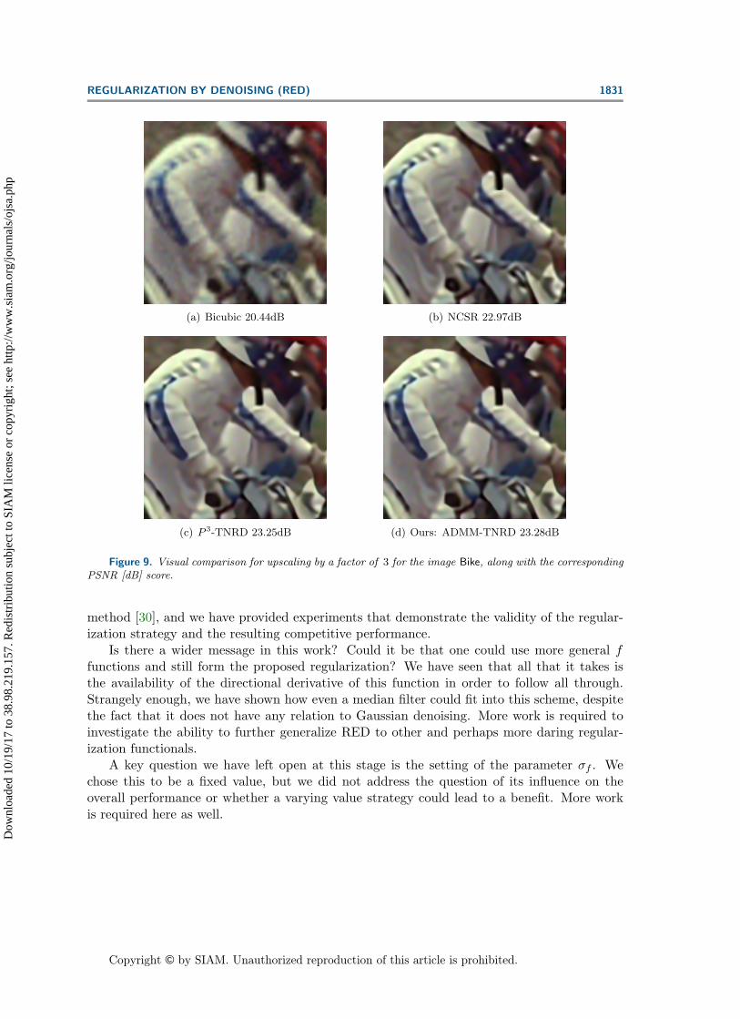
Copyright © by SIAM. Unauthorized reproduction of this article is prohibited.
REGULARIZATION BY DENOISING (RED) 1831
(a) Bicubic 20.44dB (b) NCSR 22.97dB
(c) P 3-TNRD 23.25dB (d) Ours: ADMM-TNRD 23.28dB
Figure 9. Visual comparison for upscaling by a factor of 3 for the image Bike, along with the correspondingPSNR [dB] score.
method [30], and we have provided experiments that demonstrate the validity of the regular-ization strategy and the resulting competitive performance.
Is there a wider message in this work? Could it be that one could use more general ffunctions and still form the proposed regularization? We have seen that all that it takes isthe availability of the directional derivative of this function in order to follow all through.Strangely enough, we have shown how even a median filter could fit into this scheme, despitethe fact that it does not have any relation to Gaussian denoising. More work is required toinvestigate the ability to further generalize RED to other and perhaps more daring regular-ization functionals.
A key question we have left open at this stage is the setting of the parameter σf . Wechose this to be a fixed value, but we did not address the question of its influence on theoverall performance or whether a varying value strategy could lead to a benefit. More workis required here as well.
Dow
nloa
ded
10/1
9/17
to 3
8.98
.219
.157
. Red
istr
ibut
ion
subj
ect t
o SI
AM
lice
nse
or c
opyr
ight
; see
http
://w
ww
.sia
m.o
rg/jo
urna
ls/o
jsa.
php

Copyright © by SIAM. Unauthorized reproduction of this article is prohibited.
1832 YANIV ROMANO, MICHAEL ELAD, AND PEYMAN MILANFAR
100 101 102
Iterations
25
25.5
26
26.5
27
27.5
28
28.5
29
PS
NR
RED-SDRED-FPRED-ADMM: -=0.001, m
2=1
RED-ADMM: -=0.001, m 2=3
P3: -0=0.001, ,=1.02
(a) Comparison between RED and P 3
100 101 102
Iterations
24
25
26
27
28
29
PS
NR
P3: -0=0.01, ,=1.02
P3: -0=0.001, ,=1.02
P3: -0=0.0001, ,=1.02
P3: -0=0.01, ,=1.125
P3: -0=0.001, ,=1.125
P3: -0=0.0001, ,=1.125
(b) P 3: Sensitivity to change in β0 and α
100 101 102
Iterations
25.5
26
26.5
27
27.5
28
28.5
29
PS
NR
RED-ADMM: -=0.01, m 2=1
RED-ADMM: -=0.001, m 2=1
RED-ADMM: -=0.0001, m 2=1
RED-ADMM: -=0.01, m 2=3
RED-ADMM: -=0.001, m 2=3
RED-ADMM: -=0.0001, m 2=3
(c) RED: Robustness to change in β and m2
100 101 102
Iterations
25.5
26
26.5
27
27.5
28
28.5
29P
SN
R
RED-FP: <f=3
RED-FP: <f=5
RED-FP: <f=7
(d) RED: The effect of a change in σf
Figure 10. Image super-resolution. Average PSNR as a function of the iterations of the different methods.The test images are those of Table 4.
Appendix A. Can we mimic any prior? So far we have shown that denoisers f(x) can beused to define the powerful family of priors xT (x − f(x)) that can regularize a wide varietyof inverse problems. Now, let’s consider the reverse question: For a given ρ(x), what is theeffective f(x) behind it (if any)? More specifically, given ρ(x), we wish to find f(x) such that
(50)12xT (x− f(x)) = ρ(x).
Recall that one of the key conditions we assumed for the denoiser f(x) is that it is homogeneousof degree 1,
(51) f(cx) = cf(x).
This immediately notifies us that the ρ(x) we wish to mimic in (50) must be 2-homogeneousDow
nloa
ded
10/1
9/17
to 3
8.98
.219
.157
. Red
istr
ibut
ion
subj
ect t
o SI
AM
lice
nse
or c
opyr
ight
; see
http
://w
ww
.sia
m.o
rg/jo
urna
ls/o
jsa.
php
Copyright © by SIAM. Unauthorized reproduction of this article is prohibited.
REGULARIZATION BY DENOISING (RED) 1833
because
(52) ρ(cx) =12
(cx)T (cx− f(cx)) =12c2xT (x− f(x)) = c2ρ(x).
Of course, not all priors satisfy this condition, but the class of priors that do is wide. Forinstance, while the total-variation function TV(x) = ‖∇x‖1 is only 1-homogeneous, its square‖∇x‖21 keeps us in business. More generally, since any norm is by definition 1-homogeneous,all regularizers of the type ρ(x) = ‖Ax‖2q for q = 1, 2, . . . ,∞ are 2-homogeneous:13
(53) ρ(cx) = ‖A(cx)‖2q = (c‖Ax‖q)2 = c2‖Ax‖2q = c2ρ(x).
Squared norms are not the only functions at our disposal. Beyond norms, any k-homogeneousfunction (such as homogeneous polynomials of degree k) can be made 2-homogeneous byraising to power 2/k. As well, order statistics such as maximum, minimum, and median are1-homogeneous and can be squared to the same end.
With the above discussion, we move forward with the assumption that we have a 2-homogeneous prior ρ(x) in our hands. Let’s recall that the task is to find f(x) so that
(54)12xT (x− f(x)) = ρ(x).
We proceed by differentiating both sides:
x− 12∇(xT f(x)
)= ∇ρ(x),
x− 12
(f(x) +∇f(x) x) = ∇ρ(x),
x− 12
(f(x) + f(x)) = ∇ρ(x),
x− f(x) = ∇ρ(x),
where in the last step we have invoked the directional derivative expression developed in (14).The solution, f(x), is a denoiser explicitly defined in terms of the prior,
(55) f(x) = x−∇ρ(x).
This is quite a natural result in retrospect—it resembles an SD step.14 To see this, considerthe denoising problem regularized by ρ(x):
(56) Argminx
12‖x− y‖2 + ρ(x).
One step of SD with a step-size of 1 and initial condition x0 = y would read as
(57) x1 = x0 − (x0 − y +∇ρ(x0)) = y−∇ρ(y),
13The sparsity-inspired L0 is an exception that cannot be treated this way.14It is interesting to note the resemblance of this expression to a similar expression that holds for proximal
operators (see [60]). In this context, the class of denoisers we have described using Conditions 1 and 2 is amore general form of proximal mappings.D
ownl
oade
d 10
/19/
17 to
38.
98.2
19.1
57. R
edis
trib
utio
n su
bjec
t to
SIA
M li
cens
e or
cop
yrig
ht; s
ee h
ttp://
ww
w.s
iam
.org
/jour
nals
/ojs
a.ph
p

Copyright © by SIAM. Unauthorized reproduction of this article is prohibited.
1834 YANIV ROMANO, MICHAEL ELAD, AND PEYMAN MILANFAR
just as shown above as a denoising on y.
Appendix B. Kernelizing priors. We showed in the previous section that a prior withthe right properties implies a denoiser beneath and that this denoiser is directly given by thegradient of the prior. Next, let’s address a related, but more specific question: Given a priorρ(x), does it imply a denoising filter of the pseudo-linear form f(x) = W(x)x? These typesof filters are of course of great interest because they reveal the kind of weighted averagingdone by the denoiser, and they are easy to implement. Given x, we can compute the weightsW(x) in one step and apply them as W(x)x to the image in another step. Some of the mostpopular filters to date, such as bilateral, NLM, and K-SVD, are of this convenient form.
Before we go about finding the hidden filter matrix W(x), let’s illustrate a useful propertyof the pseudo-linear filters. Take f(x) = W(x)x, and again invoke the expression f(x) =∇f(x)x developed in (14). Substitution gives
(58) W(x)x = ∇f(x)x =⇒ (∇f(x)−W(x))x = 0
for all x. From this we conclude that the gradient of pseudo-linear filters is in fact the weightmatrix
(59) ∇f(x) = W(x).
Now we can go after the weight matrix by taking the analysis from the previous sectionone step further and computing the second derivative of (50). Starting with the expression(55) that arose from the first derivative, we differentiate again,
f(x) = x−∇ρ(x),∇f(x) = I−∇(∇ρ(x)),∇f(x) = I−H(ρ(x)).
Replacing ∇f(x) = W(x), we obtain the pleasing result that the weight matrix implied bythe prior is the identity matrix minus the Hessian of the prior,
(60) W(x) = I−H(ρ(x)),
or, posed another way, L(x) = I−W(x) = H(ρ(x)) (i.e., the Laplacian filter is directly givenby the Hessian of the prior, which is not surprising, bearing in mind that we seek a relationof the form ρ(x) = xTL(x)x). What we have done here is to “kernelize” the regularizer andfind an explicit expression for the weights of the implied filter. Several observations aboutthis result are in order:
• Convexity: If ρ(x) is convex, then its Hessian is symmetric positive semidefinite(PSD), and therefore L(x) is PSD. Furthermore, if η (L(x)) ≤ 1, we get that (i) W(x)has spectral radius equal or smaller than 1, implying that strong passivity condition(Condition 2) is guaranteed; and (ii) W(x) = I − L(x) is also PSD—a desirableproperty [19].D
ownl
oade
d 10
/19/
17 to
38.
98.2
19.1
57. R
edis
trib
utio
n su
bjec
t to
SIA
M li
cens
e or
cop
yrig
ht; s
ee h
ttp://
ww
w.s
iam
.org
/jour
nals
/ojs
a.ph
p
Copyright © by SIAM. Unauthorized reproduction of this article is prohibited.
REGULARIZATION BY DENOISING (RED) 1835
• Homogeneity: Since ρ(x) is 2-homogeneous, its gradient is 1-homogeneous. We canshow this by differentiating:
ρ(cx) = c2ρ(x),∇xρ(cx) = c2∇xρ(x),
∂cx∂x∇cxρ(cx) = c2∇xρ(x),
c∇cxρ(cx) = c2∇xρ(x),∇cxρ(cx) = c∇xρ(x).
Similarly the Hessian H(ρ(x)) is invariant15 to scaling of the image x, and so is theimplied filter matrix W(x). Consequently, the applied filter W(x)x is 1-homogeneous,which again is consistent with our earlier conditions.• Row stochasticity: Let’s recall the expression we derived above for the filter in terms
of the Hessian of the prior,
(61) W(x) = I−H(ρ(x)).
If a filter defined this way is to be row-stochastic, we would have (for every x),W(x)1 = (I−H(ρ(x))) 1 = 1, or equivalently
(62) H(ρ(x))1 = 0.
This relation does not hold in general. However, consider defining the prior in termsof the gradient of the image instead of the image itself. Namely, this involves a changeof variables in the prior ρ(x) from x to Dx, where D is the gradient (e.g., difference)operator. For instance, instead of ρ(x) = ‖x‖21, consider ρD(x) = ‖Dx‖21. The Hessianof the prior under this linear transformation is given by the chain rule as
(63) H(ρD(x)) = DTH(ρ(x))D.
This Hessian, when applied to the constant vector 1, will vanish for all x, since D1 = 0:
(64) DTH(ρ(x))D 1 = 0,
so the filter resulting from this Hessian is row-stochastic. In fact, the same can be saidfor column stochasticness, since 1TDT = 0.
Appendix C. More on homogeneity. The concept of homogeneity of a filter played animportant role in the development of the key results of the paper. So it is worth saying abit more about it and to question whether this condition is satisfied for some popular andfamiliar filters.
15Or 0-homogeneous.Dow
nloa
ded
10/1
9/17
to 3
8.98
.219
.157
. Red
istr
ibut
ion
subj
ect t
o SI
AM
lice
nse
or c
opyr
ight
; see
http
://w
ww
.sia
m.o
rg/jo
urna
ls/o
jsa.
php

Copyright © by SIAM. Unauthorized reproduction of this article is prohibited.
1836 YANIV ROMANO, MICHAEL ELAD, AND PEYMAN MILANFAR
C.1. Nonlocal means and bilateral filter. A general construction of a denoising filtercould be based on a symmetric positive semidefinite kernel Ki,j(x) = K(xi, xj) ≥ 0 fromwhich the filter matrix W(x) is constructed by normalization. More specifically,
(65) Wi,j(x) =Ki,j(x)∑ni=1 Ki,j(x)
.
Whether such a denoiser is homogeneous very much depends on the choice of the kernel K.For instance, if the kernel is homogeneous of any degree p, then the resulting filter matrix isinvariant to scaling through cancellation,
(66) Wi,j(cx) =Ki,j(cx)∑ni=1 Ki,j(cx)
=cpKi,j(x)∑ni=1 c
pKi,j(x)= Wi,j(x).
Examples of homogeneous kernels include (homogeneous) polynomials and several others [45]which are not in common use in image processing. Most commonly used kernels are theexponentials (Gaussian to be exact), which are used in the bilateral or NLM cases. TheGaussian function is not homogeneous, but as we will show below, the resulting pseudo-linearfilter is nearly so. We will show that for c = 1 + ε with very small ε we have 1-homogeneityfor the NLM-type filters, namely,
(67) f(cx) = W(cx)(cx) = cW(x) x = cf(x).
The i, jth element of the filter weight matrix for the NLM filter16 is
(68) Wi,j(x;σ) =eij(σ)dj(σ)
,
where
eij(σ) = exp(−‖Rix−Rjx‖2/2σ2),
dj(σ) =n∑i=1
exp(−‖Rix−Rjx‖2/2σ2),
where Rix is a patch centered at pixel position i, extracted from the image; the normalizationconstant dj(σ) is given by summing across the rows of the kernel matrix.
Do these weights change much when the image x is replaced by a scaled version cx? First,note that if σ is nearly zero, then all weights are essentially equal to 1/n and therefore theyare automatically invariant to scaling of the image. Next, let’s consider the other extremewhere the value of σ is away from zero. Now, note that the scaling in x can be absorbed inthe parameter σ as follows:
(69) exp(−‖cRix− cRjx‖2/2σ2) = exp(−‖Rix−Rjx‖2/2(σ/c)2).
16The bilateral filter, which includes a spatial distance weight, can be treated similarly, since the spatialweights are invariant to scaling of the values of the image in any case.D
ownl
oade
d 10
/19/
17 to
38.
98.2
19.1
57. R
edis
trib
utio
n su
bjec
t to
SIA
M li
cens
e or
cop
yrig
ht; s
ee h
ttp://
ww
w.s
iam
.org
/jour
nals
/ojs
a.ph
p

Copyright © by SIAM. Unauthorized reproduction of this article is prohibited.
REGULARIZATION BY DENOISING (RED) 1837
Second, the effect of this (multiplicative) scaling can be approximated by an additive pertur-bation,
(70)σ
c=
σ
1 + ε≈ σ − εσ = σ + δ.
We now compute an approximation to Wi,j(x, σ + δ) using a Taylor series:
Wi,j((1 + ε)x;σ) ≈Wi,j(x;σ + δ)
≈Wi,j(x;σ) + δ∂Wi,j(x;σ)
∂σ.
The derivative of the weight values will be calculated in terms of the functions eij(σ) anddj(σ) as follows:
∂Wi,j(x;σ)∂σ
=∂
∂σ
(eij(σ)dj(σ)
)=e′ij(σ)dj(σ)− eij(σ)d′j(σ)
d2j (σ)
=e′ij(σ)dj(σ)
− eij(σ)dj(σ)
d′j(σ)dj(σ)
=‖Rix−Rjx‖2
σ3eij(σ)dj(σ)
− eij(σ)dj(σ)
d′j(σ)dj(σ)
=‖Rix−Rjx‖2
σ3 Wi,j(x;σ)−d′j(σ)dj(σ)
Wi,j(x;σ)
=(‖Rix−Rjx‖2
σ3 −d′j(σ)dj(σ)
)Wi,j(x;σ).
Therefore,
(71) Wi,j(x;σ + δ) ≈[1 + δ
(‖Rix−Rjx‖2
σ3 −d′j(σ)dj(σ)
)]Wi,j(x;σ).
Replacing δ = −εσ, we obtain
Wi,j((1 + ε)x;σ) ≈[1− ε
(‖Rix−Rjx‖2
σ2 − σd′j(σ)dj(σ)
)]Wi,j(x;σ)
= (1− ε φ(σ)) Wi,j(x;σ).
We can simplify further, but this is not necessary, since φ(σ) does not depend on ε. For itspart, φ(σ) behaves like n/σ2. To see this note that the first term in the definition of φ is atworst n/σ2, since ‖Rix−Rjx‖2 is bounded by n, given that the pixel values are in the range[0, 255].
Similarly, d is on the order of n · exp(‖Rix − Rjx‖2/2σ2), and its derivative d′ is onthe order of n · ‖Rix − Rjx‖2 · d/σ3. Consequently, the second term σ · d′/d behaves likeD
ownl
oade
d 10
/19/
17 to
38.
98.2
19.1
57. R
edis
trib
utio
n su
bjec
t to
SIA
M li
cens
e or
cop
yrig
ht; s
ee h
ttp://
ww
w.s
iam
.org
/jour
nals
/ojs
a.ph
p
Copyright © by SIAM. Unauthorized reproduction of this article is prohibited.
1838 YANIV ROMANO, MICHAEL ELAD, AND PEYMAN MILANFAR
‖Rix −Rjx‖2/σ2 is also on the order of n/σ2. Therefore, choosing ε = 1/n, for sufficientlylarge σ, the term εφ(σ) becomes negligible.
What we have shown is that the filter weights change very little as a result of the scaling(1 + ε)x as long as ε is very small. Therefore, the NLM (and bilateral) filters are (almostexactly) 1-homogeneous, as we had hoped.
C.2. Tikhonov regularizer and Wiener filtering. We now turn to show that Tikhonovregularization obeys the homogeneity condition. In this case, the denoised image is the solutionof
x = Argminx
12σ2 ‖x− y‖22 +
λ
2‖Bx‖22 ,(72)
where B, for example, can be a discrete approximation of a derivative operator. The closed-form expression of the above minimization is given by
x = f(y) =(I + λσ2BTB
)−1y(73)
= Wy.
When we feed this linear denoiser with the scaled image (1 + ε)y, it gives
f((1 + ε)y) =(I + λσ2BTB
)−1(1 + ε)y,(74)
which is trivially the same as (1 + ε)f(y).A more challenging case is obtained when the denoiser adapts to the input such that when
we apply f((1 + ε)y), the denoiser modifies λ to be λ(1 + ε)2. In what follows we return to(74), but this time with the modified λ, and study the behavior of the filter for infinitesimalchange in ε, i.e.,
limε→0
W(ε) = limε→0
(I + λ(1 + ε)2σ2BTB
)−1.(75)
By relying on the first-order Taylor expansion of the above expression and taking the limitε→ 0 we get the following:
W(ε) ≈W(0)− ε W(ε)(λ(1 + ε)2σ2BTB
)TW(ε)|ε=0(76)
= W− ε 2λσ2WBTBW
= (I− ε 2λσ2WBTB)W,
where W = W(0). Therefore, we obtain that the adaptive filter W(ε) changes linearly withε. Moreover, ‖σ2WBTB‖ < 1, and thus if λ� 1, the second term becomes negligible (similarto what we have shown for the NLM filter). Therefore, we conclude that the image-adaptiveWiener filtering satisfies the homogeneity condition under mild conditions.
C.3. Patch-based denoising. We now turn to discuss state-of-the-art patch-based de-noising algorithms. These methods clean the input noisy image by (i) breaking it into smalloverlapping patches, (ii) applying a local denoising step, and (iii) reconstructing the outputD
ownl
oade
d 10
/19/
17 to
38.
98.2
19.1
57. R
edis
trib
utio
n su
bjec
t to
SIA
M li
cens
e or
cop
yrig
ht; s
ee h
ttp://
ww
w.s
iam
.org
/jour
nals
/ojs
a.ph
p

Copyright © by SIAM. Unauthorized reproduction of this article is prohibited.
REGULARIZATION BY DENOISING (RED) 1839
by averaging the denoised overlapping patches to form the final image. The wisdom of thesealgorithms relies on the choice of the local nonlinear prior. Moreover, in most cases, thedenoising process can be divided into two parts; the first contains all the nonlinear decisionsmade by the prior, while the second is nothing but a linear filter that cleans the noisy patchesfollowed by a patch-averaging step. Clearly, the latter fulfills the homogeneity condition dueto its linearity. In what follows we argue that the nonlinear part of various popular denois-ers is stable to an infinitesimal change in scale, thus leading to an overall satisfaction of thehomogeneity property.
Gaussian mixture model. We start by EPLL, which can be considered as an iterativeGMM denoising algorithm. The nonlinear part of the GMM prior is the choice of a (pretrained)Gaussian model that best fits the input noisy patch, and its linear part is the subsequentWiener filtering step. Consider a Gaussian model for an n-dimensional patch xi ∼ N(0,Σk),where Σk ∈ Rn×n is the kth Gaussian, taken from the mixture. Following the derivationsin [43], the MAP estimate is formulated by
xki = Argminxi
12‖xi − yi‖22 + σ2xTi Σ−1
k xi(77)
=(I + σ2Σ−1
k
)−1yi
= Wki yi,
which is nothing but the Wiener filter that cleans the ith noisy patch yi. The best model forthe ith patch, k∗i , is the one that maximizes the MAP over all the possible models, given by
k∗i = Argmink‖xki − yi‖22 + σ2(xki )
TΣ−1k (xki ) + σ2 log |Σk|.(78)
By plugging (77) into the above we get
k∗i = Argmink‖(Wk
i − I)yi‖22 + σ2(Wki yi)
TΣ−1k (Wk
i yi) + σ2 log |Σk|(79)
= Argmink
Ψ(y, σ,Σk).
When we feed the denoiser with (1 + ε)yi, the above can be written as
k∗,εi = Argmink
(1 + ε)2‖(Wki − I)yi‖22 + (1 + ε)2σ2(Wk
i yi)TΣ−1
k (Wki yi) + σ2 log |Σk|(80)
= Argmink‖(Wk
i − I)yi‖22 + σ2(Wki yi)
TΣ−1k (Wk
i yi) +σ2
(1 + ε)2log |Σk|.
By relying on the relation 1/(1 + ε)2 ≈ 1− 2ε we further simplify the above and obtain
k∗,εi = Argmink‖(Wk
i − I)yi‖22 + σ2(Wki yi)
TΣ−1k (Wk
i yi) + σ2 log |Σk| − 2εσ2 log |Σk|(81)
= Argmink
Ψ(y, σ,Σk)− 2εσ2 log |Σk|.
Now we turn to compare (79) to the one derived above and get the following condition on εthat guarantees that k∗,εi = k∗i :
(82) Ψ(y, σ,Σk)− 2εσ2 log |Σk| > Ψ(y, σ,Σk∗)− 2εσ2 log |Σk∗ |.Dow
nloa
ded
10/1
9/17
to 3
8.98
.219
.157
. Red
istr
ibut
ion
subj
ect t
o SI
AM
lice
nse
or c
opyr
ight
; see
http
://w
ww
.sia
m.o
rg/jo
urna
ls/o
jsa.
php

Copyright © by SIAM. Unauthorized reproduction of this article is prohibited.
1840 YANIV ROMANO, MICHAEL ELAD, AND PEYMAN MILANFAR
Since Ψ(y, σ,Σk) > Ψ(y, σ,Σk∗), one can always choose ε→ 0, which will keep this inequalityintact. In an extremely rare case, when Ψ(y, σ,Σk) = Ψ(y, σ,Σk∗), we can modify the GMMdenoiser and propose a simple rule for choosing the model that has a smaller log |Σk| term,ensuring that k∗,εi = k∗i . To conclude, the nonlinear part of the GMM denoising algorithm isstable to small scaling of the input.
Sparsity-inspired denoisers: K-SVD. Given a dictionary, the nonlinear mechanism ofK-SVD is the orthogonal matching pursuit (OMP) [61] algorithm, which estimates the sparserepresentation of an input noisy patch. This is a greedy method, aiming to approximate thesolution of
αi = Argminαi‖αi‖0 s.t. ‖yi −Dαi‖22 ≤ nσ2,(83)
where n is the size of the patch, and D ∈ Rn×m is a (possibly redundant, m > n, andnonorthogonal) dictionary. At each step, denoted by k, OMP picks a new atom (a columnfrom D) that minimizes the residual. Formally, the rule for choosing the first atom dj1 canbe written as
j1 = Argmaxj|dTj yi|,(84)
while in the tth step of the OMP, it is the one that maximizes
jt = Argmaxj|dTj rti|,(85)
where rti = yi−DStiαti is the residual. We denoted by Sti the set of chosen atoms, obtained in
the previous steps, and by DSti∈ Rn×|Sti | the corresponding dictionary—a matrix having the
chosen atoms as its columns. This expression can be further simplified by relying on the factthat the representation is the outcome of a least-squares solution, given by
αti =(DTSti
DSti
)−1DTSti
yi.(86)
Substituting the above in (85) results in
jt = Argmaxj|dTj ri| = Argmax
j
∣∣∣∣dTj (I−(DTSti
DSti
)−1DTSti
)yi
∣∣∣∣ .(87)
This process is repeated until reaching the error constraint.Trivially, scaling the input patch would not modify the result of (84) and (87). However,
scaling the input may modify the stopping rule and thereby the number of atoms that theOMP picks. This will happen only when ‖yi − Dαi‖22 = nσ2, which is an extremely rarecase. Notice that given the final set of chosen atoms, S∗i , the cleaned patch is given byxi = DS∗i
(DTS∗i
DS∗i
)−1DTS∗i
yi, which clearly satisfies the homogeneity condition. To conclude,we showed that the nonlinear part of OMP is stable to an infinitesimal change in scale, andsince the cleaned patch is simply obtained by a linear projection onto the chosen atoms wehave that with high probability OMP (and thus K-SVD) fulfills our hope for homogeneity.
Dow
nloa
ded
10/1
9/17
to 3
8.98
.219
.157
. Red
istr
ibut
ion
subj
ect t
o SI
AM
lice
nse
or c
opyr
ight
; see
http
://w
ww
.sia
m.o
rg/jo
urna
ls/o
jsa.
php
Copyright © by SIAM. Unauthorized reproduction of this article is prohibited.
REGULARIZATION BY DENOISING (RED) 1841
Appendix D. The differentiability requirement. In the opening of section 3.1, we requiredthe denoising engine f(x) to be differentiable. Why? There are several benefits for havingthis behavior:
1. The directional derivative property, ∇xf(x)x = f(x), which emerges from the homo-geneity condition, becomes possible.
2. The passivity condition, which refers to the spectral radius of ∇xf(x), stands on solidground.
3. The convergence of the fixed-point algorithm discussed in section 4.2 is guaranteed.4. The convexity of the regularization term ρL(x), discussed in section 5.1 and emerging
from Condition 2, becomes possible.All these are good reasons for demanding differentiability of the denoiser f(x), and yet thequestion is whether it is too limiting or whether this requirement could be circumvented.
Observe that point 1 above could rely on the availability of a far weaker requirementof the availability of all directional derivatives of the form ∇xf(x)x. Indeed, the passivitymentioned in point 2 could also be posed in terms of a directional derivative, replacing (15)by the somewhat weaker requirement
∀x 6= 0,xT∇xf(x)x
xTx≤ 1,
under the assumption that ∇xf(x) is symmetric.The question we leave as open at this stage is whether points 3 and 4 above (convergence of
the fixed-point algorithm and the convexity of our regularization) could rely on the existenceof all directional derivatives. At worst, if indeed the denoising engine is not differentiable buthas all its directional derivatives, points 3 and 4 are lost, and the behavior of the proposedalgorithm is not clear from a theoretical standpoint.
A different and more practical question is whether a differentiability assumption on f(x) isfeasible in existing algorithms. NLM and the Bilateral filter are clearly differentiable. TNRDis differentiable as well, since its nonlinearities are smooth (linear combination of GaussianRBFs). EPLL, BM3D, and K-SVD are more challenging, since their nonlinear parts includesharp decisions. Each of these methods could be ε-modified to have a fuzzy decision, thusrendering all of them differentiable with hardly any change in their actual behavior.
REFERENCES
[1] A. Buades, B. Coll, and J.M. Morel, A non-local algorithm for image denoising, in CVPR, 2005.[2] C. Kervrann and J. Boulanger, Optimal spatial adaptation for patch-based image denoising, IEEE
Trans. Image Process., 15 (2006), pp. 2866–2878.[3] T. Tasdizen, Principal neighborhood dictionaries for nonlocal means image denoising, IEEE Trans. Image
Process., 18 (2009), pp. 2649–2660.[4] M. Elad and M. Aharon, Image denoising via sparse and redundant representations over learned
dictionaries, IEEE Trans. Image Process., 15 (2006), pp. 3736–3745.[5] K. Dabov, A. Foi, V. Katkovnik, and K. Egiazarian, Image denoising by sparse 3-D transform-
domain collaborative filtering, IEEE Trans. Image Process., 16 (2007), pp. 2080–2095.[6] H. Takeda, S. Farsiu, and P. Milanfar, Kernel regression for image processing and reconstruction,
IEEE Trans. Image Process., 16 (2007), pp. 349–366.Dow
nloa
ded
10/1
9/17
to 3
8.98
.219
.157
. Red
istr
ibut
ion
subj
ect t
o SI
AM
lice
nse
or c
opyr
ight
; see
http
://w
ww
.sia
m.o
rg/jo
urna
ls/o
jsa.
php

Copyright © by SIAM. Unauthorized reproduction of this article is prohibited.
1842 YANIV ROMANO, MICHAEL ELAD, AND PEYMAN MILANFAR
[7] J. Mairal, F. Bach, J. Ponce, G. Sapiro, and A. Zisserman, Non-local sparse models for imagerestoration, in ICCV, 2009.
[8] W. Dong, X. Li, L. Zhang, and G. Shi, Sparsity-based image denoising via dictionary learning andstructural clustering, in CVPR, 2011.
[9] W. Dong, L. Zhang, G. Shi, and X. Li, Nonlocally centralized sparse representation for image restora-tion, IEEE Trans. Image Process., 22 (2013), pp. 1620–1630.
[10] P. Chatterjee and P. Milanfar, Patch-based near-optimal image denoising, IEEE Trans. Image Pro-cess., 21 (2012), pp. 1635–1649.
[11] H.C. Burger, C.J. Schuler, and S. Harmeling, Image denoising: Can plain neural networks competewith BM 3D?, in CVPR, 2012.
[12] M. Lebrun, M. Colom, A. Buades, and J.-M. Morel, Secrets of image denoising cuisine, ActaNumer., 21 (2012), pp. 475–576.
[13] M. Lebrun, A. Buades, and J.-M. Morel, Implementation of the “non-local Bayes” (NL-Bayes) imagedenoising algorithm, IPOL, 3 (2013), pp. 1–42.
[14] C. Knaus and M. Zwicker, Dual-domain image denoising, in ICIP, 2013.[15] H. Talebi and P. Milanfar, Global image denoising, IEEE Trans. Image Process., 23 (2014), pp.
755–768.[16] S. Gu, L. Zhang, W. Zuo, and X. Feng, Weighted nuclear norm minimization with application to
image denoising, in CVPR, 2014.[17] W. Dong, G. Shi, Y. Ma, and X. Li, Image restoration via simultaneous sparse coding: Where struc-
tured sparsity meets Gaussian scale mixture, Int. J. Comput. Vis., 114 (2015), pp. 217–232.[18] N. Pierazzo, M. Rais, J.-M. Morel, and G. Facciolo, DA3D: Fast and data adaptive dual domain
denoising, in ICIP, 2015.[19] P. Milanfar, Symmetrizing smoothing filters, SIAM J. Imaging Sci., 6 (2013), pp. 263–284, https:
//doi.org/10.1137/120875843.[20] Y. Chen and T. Pock, Trainable Nonlinear Reaction Diffusion: A Flexible Framework for Fast and
Effective Image Restoration, preprint, https://arxiv.org/abs/1508.02848, 2015.[21] P. Chatterjee and P. Milanfar, Is denoising dead?, IEEE Trans. Image Process., 19 (2010), pp.
895–911.[22] A. Levin and B. Nadler, Natural image denoising: Optimality and inherent bounds, in CVPR, 2011.[23] A. Levin, B. Nadler, F. Durand, and W.T. Freeman, Patch complexity, finite pixel correlations and
optimal denoising, in ECCV, 2012.[24] M. Protter, M. Elad, H. Takeda, and P. Milanfar, Generalizing the nonlocal-means to superreso-
lution reconstruction, IEEE Trans. Image Process., 18 (2009), pp. 36–51.[25] S. Ravishankar and Y. Bresler, MR image reconstruction from highly undersampled k-space data by
dictionary learning, IEEE Trans. Med. Imag., 30 (2011), pp. 1028–1041.[26] M. Akcakaya, T.A. Basha, B. Goddu, L.A. Goepfert, K.V. Kissinger, V. Tarokh, W.J. Man-
ning, and R. Nezafat, Low-dimensional structure self-learning and thresholding: Regularizationbeyond compressed sensing for MRI reconstruction, Magn. Reson. Med., 66 (2011), pp. 756–767.
[27] A. Danielyan, V. Katkovnik, and K. Egiazarian, BM 3D frames and variational image deblurring,IEEE Trans. Image Process., 21 (2012), pp. 1715–1728.
[28] W. Dong, L. Zhang, R. Lukac, and G. Shi, Sparse representation based image interpolation withnonlocal autoregressive modeling, IEEE Trans. Image Process., 22 (2013), pp. 1382–1394.
[29] C.A. Metzler, A. Maleki, and R.G. Baraniuk, Optimal recovery from compressive measurementsvia denoising-based approximate message passing, in SAMPTA, 2015.
[30] S.V. Venkatakrishnan, C.A. Bouman, and B. Wohlberg, Plug-and-play priors for model basedreconstruction, in GlobalSIP, 2013.
[31] S.H. Chan, Algorithm-Induced Prior for Image Restoration, preprint, https://arxiv.org/abs/1602.00715,2016.
[32] S.H. Chan, X. Wang, and O.A. Elgendy, Plug-and-Play ADMM for Image Restoration: Fixed PointConvergence and Applications, preprint, preprint, https://arxiv.org/abs/1605.01710, 2016.
[33] S. Sreehari, S.V. Venkatakrishnan, B. Wohlberg, L.F. Drummy, J.P. Simmons, and C.A.Bouman, Plug-and-Play Priors for Bright Field Electron Tomography and Sparse Interpolation,preprint, https://arxiv.org/abs/1512.07331, 2015.
Dow
nloa
ded
10/1
9/17
to 3
8.98
.219
.157
. Red
istr
ibut
ion
subj
ect t
o SI
AM
lice
nse
or c
opyr
ight
; see
http
://w
ww
.sia
m.o
rg/jo
urna
ls/o
jsa.
php

Copyright © by SIAM. Unauthorized reproduction of this article is prohibited.
REGULARIZATION BY DENOISING (RED) 1843
[34] Y. Dar, A.M. Bruckstein, M. Elad, and R. Giryes, Postprocessing of compressed images via se-quential denoising, IEEE Trans. Image Process., 25 (2016), pp. 3044–3058.
[35] M.U. Sadiq, J.P. Simmons, and C.A. Bouman, Model based image reconstruction with physics basedpriors, in ICIP, 2016.
[36] A.M. Teodoro, J.M. Bioucas-Dias, and M.A.T. Figueiredo, Image restoration with locally selectedclass-adapted models, in ICIP, 2016.
[37] A. Brifman, Y. Romano, and M. Elad, Turning a denoiser into a super-resolver using plug and playpriors, in ICIP, 2016.
[38] A.M. Teodoro, J.M. Bioucas-Dias, and M.A.T. Figueiredo, Hyperspectral Sharpening Using Scene-Adapted Gaussian Mixture Priors, preprint, https://arxiv.org/abs/1702.02445, 2017.
[39] R.L. Lagendijk and J. Biemond, Iterative Identification and Restoration of Images, Springer, 1990.[40] L.I. Rudin, S. Osher, and E. Fatemi, Nonlinear total variation based noise removal algorithms, Phys.
D, 60 (1992), pp. 259–268.[41] S. Mallat, A Wavelet Tour of Signal Processing, Academic Press, 1999.[42] D. Zoran and Y. Weiss, From learning models of natural image patches to whole image restoration, in
CVPR, 2011.[43] G. Yu, G. Sapiro, and S. Mallat, Solving inverse problems with piecewise linear estimators: From
Gaussian mixture models to structured sparsity, IEEE Trans. Image Process., 21 (2012), pp. 2481–2499.
[44] A.M. Bruckstein, D.L. Donoho, and M. Elad, From sparse solutions of systems of equations to sparsemodeling of signals and images, SIAM Rev., 51 (2009), pp. 34–81, https://doi.org/10.1137/060657704.
[45] A. Vedaldi and A. Zisserman, Efficient additive kernels via explicit feature maps, IEEE Trans. PatternAnal. Mach. Intell., 34 (2012), pp. 480–492.
[46] V. Papyan, Y. Romano, and M. Elad, Convolutional Neural Networks Analyzed via ConvolutionalSparse Coding, preprint, https://arxiv.org/abs/1607.08194, 2016.
[47] A. Elmoataz, O. Lezoray, and S. Bougleux, Nonlocal discrete regularization on weighted graphs: Aframework for image and manifold processing, IEEE Trans. Image Process., 17 (2008), pp. 1047–1060.
[48] A.D. Szlam, M. Maggioni, and R.R. Coifman, Regularization on graphs with function-adapted diffu-sion processes, J. Mach. Learn. Res., 9 (2008), pp. 1711–1739.
[49] S. Bougleux, A. Elmoataz, and M. Melkemi, Local and nonlocal discrete regularization on weightedgraphs for image and mesh processing, Int. J. Comput. Vis., 84 (2009), pp. 220–236.
[50] G. Peyre, S. Bougleux, and L.D. Cohen, Non-local regularization of inverse problems, Inverse Probl.Imaging, 5 (2011), pp. 511–530.
[51] P. Milanfar, A tour of modern image filtering: New insights and methods, both practical and theoretical,IEEE Signal Process. Mag., 30 (2013), pp. 106–128.
[52] F.G. Meyer and X. Shen, Perturbation of the eigenvectors of the graph Laplacian: Application to imagedenoising, Appl. Comput. Harmon. Anal., 36 (2014), pp. 326–334.
[53] X. Liu, D. Zhai, D. Zhao, G. Zhai, and W. Gao, Progressive image denoising through hybrid graphLaplacian regularization: A unified framework, IEEE Trans. Image Process., 23 (2014), pp. 1491–1503.
[54] S.M. Haque, G. Pai, and V.M. Govindu, Symmetric smoothing filters from global consistency con-straints, IEEE Trans. Image Process., 24 (2014), pp. 1536–1548.
[55] A. Kheradmand and P. Milanfar, A general framework for regularized, similarity-based image restora-tion, IEEE Trans. Image Process., 23 (2014), pp. 5136–5151.
[56] Y. Romano and M. Elad, Boosting of image denoising algorithms, SIAM J. Imaging Sci., 8 (2015), pp.1187–1219, https://doi.org/10.1137/140990978.
[57] S. Boyd, N. Parikh, E. Chu, B. Peleato, and J. Eckstein, Distributed optimization and statisticallearning via the alternating direction method of multipliers, Found. Trends Mach. Learn., 3 (2011),pp. 1–122.
[58] M. Afonso, J. Bioucas-Dias, and M.A.T. Figueiredo, Fast image recovery using variable splittingand constrained optimization, IEEE Trans. Image Process., 19 (2010), pp. 2345–2356.
[59] M. Afonso, J. Bioucas-Dias, and M.A.T. Figueiredo, An augmented Lagrangian approach to theconstrained optimization formulation of imaging inverse problems, IEEE Trans. Image Process., 20(2011), pp. 681–695.
[60] N. Parikh and S. Boyd, Proximal algorithms, Found. Trends Optim., 1 (2014), pp. 123–231.
Dow
nloa
ded
10/1
9/17
to 3
8.98
.219
.157
. Red
istr
ibut
ion
subj
ect t
o SI
AM
lice
nse
or c
opyr
ight
; see
http
://w
ww
.sia
m.o
rg/jo
urna
ls/o
jsa.
php

Copyright © by SIAM. Unauthorized reproduction of this article is prohibited.
1844 YANIV ROMANO, MICHAEL ELAD, AND PEYMAN MILANFAR
[61] Y.C. Pati, R. Rezaiifar, and P.S. Krishnaprasad, Orthogonal matching pursuit: Recursive functionapproximation with applications to wavelet decomposition, in IEEE Asilomar Conf. Signals, Syst.Comput., 1993, pp. 40–44.
[62] E. Candes and T. Tao, The Dantzig selector: Statistical estimation when p is much larger than n, Ann.Statist., 35 (2007), pp. 2313–2351.
[63] Y. Romano and M. Elad, Improving K-SVD denoising by post-processing its method-noise, in ICIP,2013.
[64] H. Talebi, X. Zhu, and P. Milanfar, How to SAIF-ly boost denoising performance, IEEE Trans. ImageProcess., 22 (2013), pp. 1470–1485.
[65] T.M. Apostol, Calculus, 2nd ed., Vol. 1, Blaisdell, Waltham, MA, 1967.[66] S. Boyd and L. Vandenberghe, Convex Optimization, Cambridge University Press, 2004.[67] M. Elad, Sparse and Redundant Representations: From Theory to Applications in Signal and Image
Processing, 1st ed., Springer, 2010.[68] G.H. Golub and C.F. Van Loan, Matrix Computations, 3rd ed., John Hopkins University Press,
Baltimore, 1996.[69] M. Elad, B. Matalon, and M. Zibulevsky, Coordinate and subspace optimization methods for linear
least squares with non-quadratic regularization, Appl. Comput. Harmon. Anal., 23 (2007), pp. 346–367.
[70] M. Droske and A. Bertozzi, Higher-order feature-preserving geometric regularization, SIAM J. ImagingSci., 3 (2010), pp. 21–51, https://doi.org/10.1137/090751694.
[71] A. Beck and M. Teboulle, Fast gradient-based algorithms for constrained total variation image de-noising and deblurring problems, IEEE Trans. Image Process., 18 (2009), pp. 2419–2434.
[72] W. Dong, L. Zhang, G. Shi, and X. Wu, Image deblurring and super-resolution by adaptive sparsedomain selection and adaptive regularization, IEEE Trans. Image Process., 20 (2011), pp. 1838–1857.
Dow
nloa
ded
10/1
9/17
to 3
8.98
.219
.157
. Red
istr
ibut
ion
subj
ect t
o SI
AM
lice
nse
or c
opyr
ight
; see
http
://w
ww
.sia
m.o
rg/jo
urna
ls/o
jsa.
php