Dis cus si on Paper No. 11-079

The Labour Market in CGE Models

Stefan Boeters and Luc Savard

Dis cus si on Paper No. 11-079

The Labour Market in CGE Models

Stefan Boeters and Luc Savard

Die Dis cus si on Pape rs die nen einer mög lichst schnel len Ver brei tung von neue ren For schungs arbei ten des ZEW. Die Bei trä ge lie gen in allei ni ger Ver ant wor tung

der Auto ren und stel len nicht not wen di ger wei se die Mei nung des ZEW dar.

Dis cus si on Papers are inten ded to make results of ZEW research prompt ly avai la ble to other eco no mists in order to encou ra ge dis cus si on and sug gesti ons for revi si ons. The aut hors are sole ly

respon si ble for the con tents which do not neces sa ri ly repre sent the opi ni on of the ZEW.

Download this ZEW Discussion Paper from our ftp server:

http://ftp.zew.de/pub/zew-docs/dp/dp11079.pdf

Non-technical summary

In this chapter (writen for the forthcoming “Handbook of CGE Modeling”, editedby P.Dixon and D. Jorgenson), we review options of labour market modelling inthe framework of numerical general equilibrium analysis. Our review is structuredin three main sections: Modelling options for labour supply, labour demand andlabour market coordination.

On the labour supply side, two principal modelling options are distinguished anddiscussed: aggregated, representative households and microsimulation based on indi-vidual household data. Microsimulation is a forceful instrument, which has a numberof clear advantages (direct link to modern labour supply estimation, explicitness indistributional questions) and avoids a number of typical problems that arise in de-termining the characteristics of representative households. Therefore, in our view,any labour-market related study should carefully check whether the microsimulationset-up can be made use of.

On the labour demand side, we focus on the substitution possibilities betweendifferent types of labour in production. Labour supply analysis suggests a largenumber of potentially interesting labour subgroups. Except for a very small subsetof these, the econometric basis for formulating labour demand in these categories isweak. We think that in general the assumption of perfect substitutability in demand(implying an efficiency-weighted additive treatment of individual labour quantities)is a plausible default. Demand for different categories of labour should only bedifferentiated if there is evidence that wages do not move in parallel.

Modelling labour market coordination presents itself as a sharp trade-off. Ideally,we would like to have a theoretically founded, structural model of involuntary unem-ployment, which contains enough free parameters to be calibrated to empirical wagecurve elasticity parameters. This is not easily available. Any reasonably simple struc-tural model of unemployment has severe difficulty to be calibrated to empiricallyplausible wage curve elasticities. Working with these elasticities directly, without astructural foundation, is possible, but reduces our resources of providing an economicinterpretation of changes in the wage as a response to policy shocks.

Zusammenfassung

Dieses Kapitel (geschrieben für das “Handbook of CGE Modeling”, herausgegebenvon P.Dixon und D. Jorgenson) enthält eine Bestandsaufnahme von Modellierungs-optionen für den Arbeitsmarkt im Rahmen einer numerischen allgemeinen Gleichge-wichtsanalyse (CGE). Wir strukturieren diese Bestandsaufnahme in drei große Teile:Arbeitsangebot, Arbeitsnachfrage und Arbeitsmarktkoordination.

Auf der Arbeitsangebotsseite lauten die beiden prinzipiellen Modellierungsoptio-nen: aggregierte, representative Haushalte und Mikrosimulation auf der Basis von In-dividualdaten. Im Rahmen einer CGE-Analyse hat Mikrosimulation eine Reihe vonVorteilen (direkter Bezug zu empirischen Arbeitsangebotsschätzungen, Explizitheitin Verteilungsfragen) und vermeidet Probleme, die typischerweise bei der Bestim-mung der Eigenschaften aggregierter Haushalte auftreten. Wir sehen sie deshalb alsdas für viele Arbeitsmarktfragestellungen gebotene Instrument an.

Auf der Arbeitsnachfrageseite ist das im Rahmen einer CGE-Analyse kritischeElement die Substituierbarkeit von verschiedenen Typen Arbeit. Die Arbeitsange-botsanalyse legt eine große Zahl möglicher Arbeitsklassifikationen nahe. Nur für diewenigsten davon gibt es eine empirisch gesicherte Basis für die Nachfragebedingun-gen. In unseren Augen sollte der Ausgangspunkt einer Nachfragemodellierung im-mer vollständige Substituierbarkeit (Effizienzgewichtete Addition unterschiedlicherTypen Arbeit) sein, es sei denn es gibt empirische Belege dafür, dass die relativenPreise auf ein Auseinanderlaufen des Angebots systematisch reagieren.

Bei der Modellierung der Arbeitsmarktkoordination sehen wir uns einem Di-lemma gegenüber. Idealerweise würden wir ein theoretisch fundiertes, strukturellesModell unfreiwilliger Arbeitslosigkeit verwenden, das hinreichend freie Parameterenthält, so dass es auf empirische Lohnelastizitäten kalibriert werden kann. DiesesIdeal ist bislang in der Modellierung nicht erreicht. Einfachen strukturelle Modellenfehlt es an der Flexibilität der empirischen Anpassung, während das direkte Arbeitenmit empirischen Elastiziäten die ökonomische Interpretation von Löhnänderungenals Resultat von Veränderungen der Umgebungsvariablen erschwert.

The Labour Market in CGE Models§

written as a chapter for the “Handbook of CGE Modeling”

(eds. P. Dixon and D. Jorgenson)

Stefan Boeters∗

CPB, Netherlands Bureau for Economic Policy Analysis, Den Haag

Reseach Fellow, Centre for European Economic Research, Mannheim

Luc Savard∗∗

Université de Sherbrooke

October 2011

Abstract

This chapter reviews options of labour market modelling in a CGE frame-

work. On the labour supply side, two principal modelling options are distin-

guished and discussed: aggregated, representative households and microsim-

ulation based on individual household data. On the labour demand side, we

focus on the substitution possibilities between different types of labour in

production. With respect to labour market coordination, we discuss several

wage-forming mechanisms and involuntary unemployment.

Keywords: computable general equilibrium model, labour market, labour

supply, labour demand, microsimulation, involuntary unemployment

JEL Code: C68, D58, J20, J64

§We thank Peter Dixon, James Giesecke, John Hutton, Egbert Jongen, Andreas Peichl, Se-bastian Siegloch and Peter Sørensen for helpful comments on earlier versions of this chapter.

∗Stefan Boeters, CPB, P.O. Box 80510, 2508 GM Den Haag, Netherlands, e-mail:s.boeters@cpb.nl

∗∗Luc Savard, Department of Economics, Université de Sherbrooke, 2500, boulevard de l’Univer-sité, Sherbrooke (Québec), J1K 2R1, Canada, e-mail: luc.savard@usherbrooke.ca

1 Introduction

If we look at the body of CGE literature as a whole, the labour market has certainlynot been one of the main points of attention. In fact, many of the classical CGEstudies in the areas of trade liberalisation, tax analysis and climate policy work withthe simplest possible set of assumptions about the labour market: labour supplyis fixed and a uniform, flexible, market-clearing wage balances labour supply anddemand. The authors of these classical studies apparently did not fear to introducea serious bias into their analysis when treating the labour market in this simplifiedmanner. And they may have been right. Even if one is convinced that the reallabour market is much more complex than our simplifying model, this does notautomatically mean that its full complexity must show in every concrete analysis.Engaging in a more detailed modelling of the labour market is only worth the whileif it can be made plausible that assumptions about the labour market mechanismsactually change the outcome of a particular study significantly. Given that in amodelling context we are bound to work with simplifications anyway, we see theburden of proof with those claiming that this is the case.

There are two typical – and quite distinct – constellations that motivate research-ers to go beyond the basic set-up of a labour market clearing, flexible wage. Theyeither want to analyse a specific change in the labour market institutions, or theyare interested in the labour market consequences of a policy measure which is notdirectly labour-market related. As an example of the first motivation, take the caseof in-work benefits, which are supposed to increase labour supply of the low skilled.Addressing this issue in a CGE model requires a mechanism which endogenises la-bour supply and a labour-market segmentation which separates the low-skilled fromother groups. Thus a certain level of labour-market complexity is necessary. Thesecond motivation can be illustrated by the analysis of trade liberalisation. Thisaffects the labour market only indirectly, but we can ask about the aggregate con-sequences – What are the effects on wages and unemployment? – as well as aboutdistributional effects: Who gains and who loses? We give a more extensive overviewof motivating issues in Section 2.

Apart from these question-driven approaches to labour market modelling, thereis also an approach that one could call “presentation-driven”. Say, you work in the

1

field of climate policy analysis – an issue that is neither intrinsically labour-marketrelated nor likely to have significant effects on the labour market. However, whenyou present your results, they are called into doubt, because “your model doesn’teven allow for involuntary unemployment” (which, as everyone admits, is a worri-some feature of most economies). Trying to convince your audience that includingunemployment does not make much of a difference would divert the discussion fromthe main issue and might be difficult after all. So it can be a sensible strategy to adda more complex labour-market module to the model, if only to prevent people fromdigressing. A similar constellation can be found “history-driven” when modellersstart off from an existing model containing labour market features that are irrelev-ant for the question at hand, but would require some effort to eliminate. In bothpresentation- and history-driven contexts, we want to make sure that the labour-market features present in the model do not complicate the interpretation of theresults unnecessarily by producing spurious effects.

We fully recognise that model development in practice works under many re-strictions that are not strictly academic. This is what we have often experienced inthe work with our own models as well. Nevertheless, as economists, our thinkingis dominated by the question-driven approach. In this chapter, we want to advoc-ate and support a “question precedes model” strategy. In our view, the ideal set-upof a CGE study is the following. First, we need to formulate a clear question tobe answered, preferably more specific than merely “analysing the consequences ofpolicy X”. Often we can get, simply by phrasing the question clearly, a good ideaof which model features will be relevant to the outcome, and which will not. It is aquestion of modelling efficiency to focus on the first, and to disregard the latter.

Stated broadly, this chapter has two objectives: (1) giving an overview of whatoptions there are for labour market modelling in a CGE framework, (2) discussingadvantages or disadvantages of these options, depending on the modelling context.The structure of the chapter is derived from the three major parts of any labour mar-ket module – labour supply, labour demand and market coordination – and fromtwo directions of model development: refinement of mechanisms and disaggrega-tion of units. With respect to labour supply, we primarily focus on the distinctionbetween the representative-household and microsimulation approaches. Concerninglabour demand, substitutability and complementarity of different types of labour

2

in production are centre stage. Finally, when it comes to labour market coordina-tion, we review different theories of imperfectly competitive labour markets. – Thesecond structuring dimension distinguishes between two strands in the developmentof labour market modelling: more complex mechanisms and a deeper disaggrega-tion. Starting from the default option of almost all first-generation CGE models –market-clearing wages in a single labour market – we can in principle develop inboth directions independently: (a) more complex mechanisms, say endogenous un-employment, at the same level of aggregation, or (b) the same, simple mechanismat a deeper level of disaggregation.

In many cases, however, there are interactions between complexity and disag-gregation, which we will explore in this chapter as well. Let us illustrate this bythree examples. (1) The introduction of involuntary unemployment confronts uswith characteristically different unemployment rates for different groups of workers,which leads us to treat these labour market segments separately. (2) We find that animportant mechanism of labour market coordination – collective wage bargaining– is only relevant to particular sectors, which requires us to think about sectorallabour mobility. (3) The differentiation between male and female labour supply,which is necessary if we want to do justice to empirical labour supply elasticities,raises questions about the substitutability of male and female work in production.We must always be aware of the fact that introducing a new model feature, whichmay be well motivated in a certain context, can create loose ends at other points inour model.

We try to give a comprehensive overview of modelling options, but in some re-spects we have been selective. First, we mainly focus on issues that can be treatedin static or recursively dynamic models. Problems that require a dynamic modelwith forward-looking agents, such as life-cycle decisions like educational choice andthe timing of retirement, are not covered. Second, business-cycle issues, such as therole of sticky wages in the propagation of shocks (new Keynesian features typic-ally covered in DSGE models), are beyond the scope of this chapter. Finally, weconcentrate on models at the national or multi-national level and disregard specialproblems of factor mobility that arise in regional modelling.

3

2 A classification of labour-market related questions

In the introduction, we have advocated the perspective of seeing models as tools toanswer questions. The most straightforward type of question is: “What effect willpolicy intervention X have on economic indicator Y?” Depending on which kindof policy intervention and which kind of economic indicator we have in mind, thecriteria for an assessment of CGE labour market modelling may vary significantly.In this section, we look more systematically at the types of questions that havebeen addressed with CGE models. This results in a classification that is used forstructuring a list of typical CGE studies with a labour market focus.

Location of the initial shock

It is important to be clear about the location where the initial policy shock entersthe model. Does it affect the labour market directly or only indirectly through otherelements of the model? Let us return to the examples mentioned in the introduction.Take the case that we want to analyse the macroeconomic consequences of a policyencouraging labour supply of low-skilled workers, e.g. some in-work benefit system.Then we need a labour market module that is sufficiently complex for the policyshock to be meaningfully modelled. In this case this means that labour supply mustbe flexible and the low-skilled must be treated as a separate group.

Many of the big themes of CGE modelling, in contrast, are not directly labour-market related. International trade liberalisation hits export and import markets,climate policy measures affect energy markets, and the impact of both policies onthe labour market is only indirect through a shift in labour demand, i.e. in thereal wages that can potentially be paid to the workers at a given level of employ-ment. The same applies to tax policy analysis, as far as it is concerned with capitaltaxation, corporate taxation, intermediate input taxes or consumption taxes. Theonly exemption is wage taxation, which needs a labour market representation withflexible labour supply and heterogeneous wages for a meaningful analysis.

In all cases in which the labour market is only affected indirectly through labourdemand, we are confronted with the following key question: Will the real wagefollow the movement of the marginal product of labour one-to-one, as it would

4

in a perfect labour market? Or is there some sort of wage rigidity that hinders aparallel movement? Put into even more policy-relevant terms: To what extent willhigher demand for labour translate into higher wages, and to what extent into moreemployment (and vice versa for lower labour demand)? What is asked for is a “wagecurve”, i.e. a functional relationship between unemployment and the wage, whichthen in turn determines the wage-employment split. We return to the issue of thewage curve in Section 5.3, where we review different options of modelling imperfectlabour markets.

Outcome variables of interest

Just as important as the location of the initial shock is the outcome variable we areinterested in. Potential outcome variables of CGE models can be classified accord-ing to the level of aggregation they require. At one extreme of the spectrum, wehave typical macro variables, which give us an impression of the overall economiceffect of the policy measure analysed: GDP, national income, exports and imports,consumption and investment, or a welfare measure such as the Hicksian equivalentvariation. At an intermediate level of aggregation, we have sectoral effects: output,employment, productivity, exports and imports by sector, which are prominent inmany core issues of CGE modelling (e.g. trade liberalisation, climate policy). In thischapter, however, they are only of interest in so far as they affect the labour market.Labour market variables with a comparable, intermediate level of aggregation aregroup-specific outcomes such as wages, participation, employment and unemploy-ment by skill group or gender. Finally, if the model allows for full disaggregation,we have the additional option of reporting these variables by socio-demographicattributes that have no functional role in the labour market mechanism modelled,e.g. income class, age, education or number of children. This kind of reporting isnormally motivated by distributional concerns.

Unlike the location of the initial shock, the outcome variables used will notdirectly constitute a classification criterion of studies. The criterion is rather whethera model encompasses both the macro and the micro level. If it does, this will normallyalso be reflected in the reporting of results.

5

A classification of typical studies

Let us categorise a number of typical CGE studies with a labour market focusaccording to the criteria developed in the preceding paragraphs: Where is the policyshock located? Does the model contain a genuine micro level?

We start, in roughly chronological order, with studies that focus on labour market

shocks:

• Early attempts of addressing labour market issues in a CGE framework areGelauff et al. (1991) and Dewatripont et al. (1991), who analyse labour tax-ation and social security contributions in the Netherlands and Belgium, re-spectively.

• Sørensen (1997) studies options of stimulating low skilled employment (tax cutfor low incomes and consumption tax relief on low-skilled intensive services)in a model calibrated to the Danish economy.

• Hutton and Ruocco (1999), and Böhringer et al. (2005) analyse changes in la-bour taxation with an aggregated labour market module. The wage generatingmechanism is efficiency wages in the first paper and collective bargaining inthe latter.

• Bovenberg et al. (2000) focus on tax reform as well, but in a model that allowsfor more dimensions of labour market heterogeneity. A full-fledged version oftheir model for the Dutch economy is presented in Graafland et al. (2001).

• Aaberge et al. (2004), Arntz et al. (2008) and Boeters (2010) are examples ofintegrating microsimulation elements with a focus on re-financing the pensionsystem, stimulation of low-skilled employment and tax progressivity, respect-ively.

• Agénor et al. (2007) simulate various labour market policy measures (reductionin payroll taxation, cuts in public sector wages and employment, reductionin trade unions’ bargaining power) in a model with a dual labour marketand collective wage bargaining for a stylised Middle-East or North-African

6

economy. Agénor and El Aynaoui (2003) is an application of this model toMorocco.

• Cogneau and Robilliard (2008) set up a linked microsimulation-CGE modelof Madagascar for analysing poverty alleviation policies such as agriculturalsubsidies, a workfare scheme and untargeted per capita transfers.

• Dixon et al. (2011) study the labour market effects of restricting employmentof illegal immigrants in the U.S. by either stricter border controls or higherfines for employers.

A second set of CGE studies, again in roughly chronological order, analyse policy ormacroeconomic shocks that do not directly hit the labour market, but neverthelesshave effects on employment and distribution that depend on the labour marketspecification:

• Ballard et al. (1985) is a classical study on tax policy. Their discussion oflabour-market issues, however, is restricted to choosing an appropriate valueof the aggregated elasticity of labour supply.

• The study of de Melo and Tarr (1992) has a seminal status for the analysis oftrade liberalisation. As a specific labour market feature, they introduce wagebargaining in the automobile sector, which naturally leads them to a kind ofdual-labour-market structure.

• The trade liberalisation issue has been linked to poverty analysis in modelsthat use a full microsimulation-CGE linkage, e.g. Hérault (2007) for SouthAfrica, Bourguignon and Savard (2008) for the Philippines and Bussolo et al.(2008) for Latin America.

• Fæhn et al. (2009) and Fraser and Waschik (2010) are two studies from thefield of energy economics and climate policy analysis that have a special focuson the interactions of energy and labour markets.

• The impact of macroeconomic shocks such as financial or currency crises isanalysed in Ferreira et al. (2008) for Brazil and in Robilliard et al. (2008) forIndonesia.

7

3 Labour supply

According to the sketch in the introduction, labour supply modelling can developtowards a higher degree of complexity in two ways: (1) more subtle labour supplymechanisms and (2) a lower level of aggregation. The structure of this section isderived from the aggregation dimension. We start at the most aggregated level of asingle representative household (Section 3.1) and show how basic calibration taskscan be approached: (a) implementing empirically plausible labour supply elasticities,(b) differentiating labour supply along the intensive and extensive margin, and (c)allocating involuntary unemployment. In Section 3.2, we discuss the changes result-ing from the existence of several representative households instead of a single one.Finally, in Section 3.3, we turn to microsimulation, where labour supply is imple-mented at the lowest possible aggregation level, i.e. at the level of the individualhousehold.

3.1 Labour supply of a single representative household

At the level of a single representative household, unbothered by disaggregation is-sues, we can concentrate on the task of modelling labour supply in a way thatis consistent with given empirical elasticities. In many classical CGE models (e.g.Dervis et al., 1982), in addition to working with a single representative household, itis assumed that the labour supply of this household is fixed. Once we want to modelflexible labour supply, we are confronted with a crucial distinction. Labour supplyis flexible along two margins: hours of work (intensive margin) and participation(extensive margin). In this section, we show how labour supply of a representativehousehold can be calibrated to a set of three aggregate labour supply elasticities: (a)elasticity of participation with respect to the wage, (b) elasticity of working hourswith respect to the wage, (c) elasticity of working hours with respect to (non-wage)income. The calibration is performed by determining the parameters of a conven-tional utility function comprising material consumption and leisure.1

1The following material is adapted to the present context from Boeters and van Leeuwen (2010).

8

3.1.1 Hours of work

We consider a worker household that must decide on its hours of work under abudget constraint and a time constraint. The budget constraint is

pC (CD + C0) = wH (1− ta) + Y0

where pC is the consumption price index, CD and C0 are disposable and necessaryconsumption, respectively, w is the wage rate, H is hours of work, ta is the averagetax rate on labour income, and Y0 is non-labour income.2 The time constraint is

F + H = T

with leisure F and time endowment T. The choice of the worker household is mod-elled as the maximisation of a utility function that covers disposable consumptionand leisure, Ue = Ue (CD, F ). As our task is to determine concrete functional para-meters, we assume a CES utility function3 with parameters θC and σ

Ue =

[θC

(CD

CD

)σ−1σ

+ (1− θC)

(F

F

)σ−1σ

] σσ−1

(1)

From this utility function, we can derive the following expenditure and demandfunctions, where variables with an upper bar denote initial (and thus constant)values:

pU =

[θCp1−σ

C + (1− θC)

(w (1− tm)

w (1− tm)

)1−σ] 1

1−σ

CD

CD

= Ue

(pU

pC

)σ

F

F= Ue

(pU

w (1− tm)

w (1− tm)

)σ

2Compared to the simplest possible textbook example of labour supply, this formulation containsthree extensions that are important for empirical calibration: necessary consumption, non-labourincome and a variable average tax rate, which causes average and marginal tax rates to diverge.As we focus on static models, we do not extend the model with savings (see Rutherford (1998) forthe joint calibration of labour supply and savings).

3We use the “calibrated share form” of the CES function, see Rutherford (1998). By expressingall quantities and prices as multiples of the initial values, this form clearly conveys the ideas thatquantity normalisations are arbitrary and that the essential information is about relative changes.In addition, the value shares in the initial situation can without transformation be used as shareparameters of the function.

9

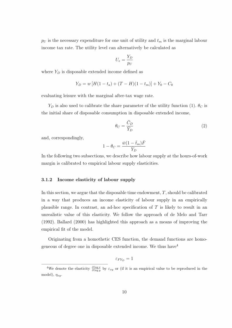
pU is the necessary expenditure for one unit of utility and tm is the marginal labourincome tax rate. The utility level can alternatively be calculated as

Ue =YD

pU

where YD is disposable extended income defined as

YD = w [H(1− ta) + (T −H)(1− tm)] + Y0 − C0

evaluating leisure with the marginal after-tax wage rate.

YD is also used to calibrate the share parameter of the utility function (1). θC isthe initial share of disposable consumption in disposable extended income,

θC =CD

YD

(2)

and, correspondingly,

1− θC =w(1− tm)F

YD

In the following two subsections, we describe how labour supply at the hours-of-workmargin is calibrated to empirical labour supply elasticities.

3.1.2 Income elasticity of labour supply

In this section, we argue that the disposable time endowment, T , should be calibratedin a way that produces an income elasticity of labour supply in an empiricallyplausible range. In contrast, an ad-hoc specification of T is likely to result in anunrealistic value of this elasticity. We follow the approach of de Melo and Tarr(1992). Ballard (2000) has highlighted this approach as a means of improving theempirical fit of the model.

Originating from a homothetic CES function, the demand functions are homo-geneous of degree one in disposable extended income. We thus have4

εFYD= 1

4We denote the elasticity ∂ log x∂ log y by εxy or (if it is an empirical value to be reproduced in the

model), ηxy.

10

From this we can derive the income elasticity of labour supply. To be precise, wecalculate the per cent change in labour supply with respect to an exogenous variationof the non-labour income, Y0, that would increase Y = wH(1 − ta) + Y0 by onepercent, if labour supply did not react.

ηHY = εHY0

Y

Y0

= εHF εFYD

dYD

dY0

Y

YD

We have

εHF = −T −H

H

εFYD=

dYD

dY0

= 1

and therefore

ηHY = −T −H

H

Y

YD

= −T −H

H

wH(1− ta) + Y0

w [H(1− ta) + (T −H)(1− tm)] + Y0 − C0

We treat ηHY as a parameter that we can observe empirically, and we use it todetermine T, the (unobservable, disposable) time endowment. Solving for T, as amultiple of initial labour supply, gives

T

H=

[wH(1− ta) + Y0]− ηLY (w [H(1− ta)−H(1− tm)] + Y0 − C0)

[ηHY wH(1− tm)] + wH(1− ta) + Y0

= 1− ηHY [wH(1− ta) + Y0 − C0]

ηHY wH(1− tm) + wH(1− ta) + Y0

(3)

For small, negative values of ηHY , T > H is warranted. At the same time, smallabsolute values of ηHY will result in a small amount of disposable leisure. In asimplified benchmark case with Y0 = C0 = 0 and proportional taxes (tm = ta = t),

eq. (3) reduces toT

H= 1− ηHY

1 + ηHY

=1

1 + ηHY

(4)

If we follow Ballard (2000) and set ηHY to the empirically plausible value of −0.1, wearrive at T/H ≈ 1.1. This may seem overly little: only 4 hours of disposable leisurein relation to a standard work week of 40 hours. In ad-hoc specifications, one oftenfinds a value of 1.75 (e.g. Rutherford, 1998). However, this would lead to incomeelasticities of labour supply which are far beyond what we empirically observe.5

5Equivalently to calibrating the time endowment T , we can also set some arbitrary time endow-

11

3.1.3 Wage elasticity of labour supply

With the relative time endowment, T/H, determined by the income elasticity oflabour supply, we proceed with calibrating the value of the elasticity of substitutionbetween material consumption and leisure, σ, using the wage elasticity of laboursupply6, ηHw, which is calculated as

ηHw = εHw = −T −H

HεFw

where w = w(1− tm). The elasticity of leisure demand with respect to the marginalafter-tax wage can be routinely decomposed into a substitution effect and an incomeeffect. The income effect deserves attention, because we need the effect of the wageon the disposable extended income, YD.

ηHw = −T −H

H

[−σθC − (1− θC) +

w(1− tm)T

YD

]Solving for σ gives the calibration equation

σ =ηHw − T−H

H

((1− θC)− w(1−tm)T

YD

)T−H

HθC

(5)

To get a feeling for magnitudes, we again consider the special case with Y0 = C0 = 0

and tm = ta. Then we havew(1− tm)T

YD

= 1

and eq. (5) simplifies to

σ =ηHw + T−H

HθC

T−HH

θC

= 1 +ηHw

T−HH

θC

(6)

Further simplification of eq. (6) is achieved by observing that in this case

θC =H

T,

ment (say, 24 hours a day) and calibrate a minimum level of leisure in the fashion of a Stone-Gearyutility function. This approach has been taken in Annabi (2003), although without discussion ofthe consequences for the income elasticity of labour supply.

6To be precise, we deal with the elasticity of the hours of work with respect to the marginalafter-tax wage. Differently specified elasticities require modifying the calculations accordingly.

12

which yields7

σ = 1 +T

T −HηHw

Finally, we insert eq. (4), which leaves us with

σ = 1− ηHw

ηHY

This shows that the inclusion of ηHY in the calibration makes the outcome for σ morevolatile. With an exogenous, relatively large T/H ratio, a small value of ηHw wouldhave warranted a small deviation of σ from one. With ηHY additionally appearing inthe equation, σ can easily assume much higher values. To get a feeling for numericalvalues, we follow Sørensen (1999) and set ηHw to 0.1.8 Together with ηHY = −0.1

(as in Section 3.1.2), this produces σ = 2.

Alternatively, it would be possible to calibrate the model to the compensatedand uncompensated elasticities of labour supply. Ballard and Fullerton (1992) usevalues of 0.2 and 0 in their benchmark case.

3.1.4 Labour supply: participation

When we proceed to the calibration of labour supply along the extensive margin(participation), we can no longer base our work on the fiction that the representativehousehold represents a large number of identical individuals. The simplest way ofimplementing the difference between participating and non-participating householdsis to assume heterogeneity in their fixed cost of taking up work. Those with low fixedcosts enter the labour market, whereas those with high fixed costs stay at home.9 Itis not necessary to specify the precise nature of these fixed costs. They may consistof costs that are caused by the difficulties of family coordination if both partnershave a paid job, commuting costs between home and work, or simply some kindof labour market attachment, an inherent utility from interacting with others in aproductive environment.

7This is also what you get in Rutherford (1998), if you leave out the upper nest with theconsumption-savings decision (assuming that the savings rate is zero).

8The meta analysis of Evers et al. (2008) suggests a somewhat higher elasticity, but it is difficultto distil a core value from this study.

9For a general discussion of this approach, see Bourguignon and Magnac (1990), Magnac (1991),Kleven and Kreiner (2006a).

13

The two-step labour-supply decision (participation, hours of work) is solved back-wards: First the individuals determine the optimal choice of hours assuming thatthey participate, then they compare this optimal outcome with the fixed cost ofworking. Things become slightly more complicated if there is involuntary unemploy-ment. A possible assumption is that individuals draw a comparison between the(unemployment-weighted) expected utility of supplying labour and their respectivefixed costs. In the case of unemployment (index u), utility is

Uu =

[θC

(Cu

D

CD

)σ−1σ

+ (1− θC)

(T

F

)σ−1σ

] σσ−1

, (7)

where disposable consumption in the case of unemployment, CuD, is income less

necessary consumption

CuD = Y u

D = cwH (1− ta) + Y u0 − C0

and unemployment benefits are assumed to be a fixed replacement rate, c, multipliedwith the after-tax income of the employed workers, wH (1− ta). The formulation (7)creates a problem, however. All relevant variables in this equation are fixed, eitherinstitutionally (c, ta) or through the calibration of the labour supply decision of theemployed workers (θC , σ, T ). For a reasonable unemployment model, we must haveUu < Ue, which is not automatically warranted. If several factors interact, Uu mayturn out to be larger than Ue: As an outcome of the calibration (see Sections 3.1.2and 3.1.3), F is typically only a small share of T, and the elasticity of substitution,σ, is considerably larger than one. Both these facts contribute to a high utilitylevel of the unemployed. On the other hand, we have basic consumption, C0, whichmakes the relative difference between Cu

D and CD larger than simply given by thereplacement rate. If the first factor dominates, we end up with a utility reversal.

Finding a solution to this problem would require further exploring the value ofinvoluntarily unemployed time, which seems to be an unresolved question in laboureconomics. The model can in principle easily be adjusted in order to allow for moreflexibility. As it stands, the parameters of the utility function have been calibratedlocally at the point where the employed workers supply labour. However, there isno strong reason to assume that the outcome of the calibration is also informativewith respect to the utility difference between two distant points, Ue − Uu. We can

14

approach the utility reversal problem by introducing an additional parameter. Thisparameter allows for the possibility that unemployed workers cannot consume theirtotal time endowment, T, as leisure. We can think of different reasons for this:Searching for a job requires time, even more so if the unemployed are expectedto attend active labour market measures. A correction factor for disposable leisurecould also capture effects of the social embeddedness that the work sphere supplies.However, it is particularly difficult to quantify this effect.10 In general terms, wemay assume that a given fraction, δ, of the additional non-working time of theunemployed does not count as “leisure”:

Uu =

[θC

(Cu

D

CD

)σ−1σ

+ (1− θC)

(T − δH

F

)σ−1σ

] σσ−1

Given Uu, with the implied difficulties, we can calculate the expected utility ofsupplying labour, Ul,

Ul = (1− u)Ue + uUu

which is the same for all individuals. They compare it with their idiosyncratic fixedcost of supplying labour, U0, and supply labour if Ul > U0.

The distribution of the U0’s over the population must be calibrated. As ourempirical basis, we have the actual participation rate and the elasticity of laboursupply at the extensive margin. This is sufficient to calibrate the distribution ofthe fixed costs locally (at the point of actual participation), but not globally. Therest of the distribution must be fixed by some functional assumption. A relativelysimple assumption is that costs are uniformly distributed between U−

0 and U+0 .

For fixing the values of these bounds, we first have to calculate the change in Ul

caused by an exogenous variation in the wage. We consider the case of an isolatedchange in the wage of the respective individuals when they are employed. In thiscase, the unemployment rate and the utility from unemployment can be considered

10A possible line of investigation would be whether there are time-use studies that inform usabout how much time the unemployed actually spend on searching. Jenkins and Montmarquette(1979) is a coarse trial to find indirect ways for evaluating unemployed time.

15

constant.11 In terms of elasticities, we then have

εUl,w =(1− u)Ue

Ul

εUe,w =(1− u)Ue

Ul

(εYD,w − εpU ,w)

=(1− u)Ue

Ul

(wT (1− tm)

YD

− wF (1− tm)

YD

)=

(1− u)Ue

Ul

wH(1− tm)

YD

The elasticity of labour supply at the extensive margin can be calculated as

ηNw = εN,UlεUl,w = h

(1− u)Ue

N

wH(1− tm)

YD

,

where h is the density of the fixed cost distribution and N is the number of parti-cipating individuals. Solving for h, we obtain

h = ηNwNYD

(1− u)UewH(1− tm). (8)

Given a particular value for ηNw,12 h can be evaluated at the initial point, andthen treated as a constant in the counterfactual simulations. This means that theelasticity at the extensive margin is precisely reproduced only for the initial point;after the initial situation, it is endogenous.

The bounds of the uniform distribution for h can be determined as

U−0 = Ul −

N

h

U+0 = Ul +

N0 − N

h

where N0 is the total population and N is initial participation. Finally, counterfac-tual participation can be calculated as

N = N + h(Ul − Ul) (9)

11This would not be the case for a general change in the wage, which applies to all individuals.12Kleven and Kreiner (2006b, p.18-20) survey the current state of empirical evidence on the

elasticity at the extensive margin. It is particularly difficult to calibrate a model with a repres-entative agent to these elasticities, because they differ considerably by household type. One mightchoose a value of 0.2, which is roughly the aggregate average in Kleven and Kreiner’s core scenario.

16

3.1.5 Supply of different labour varieties

So far, we have assumed that the labour supplied by the representative household ishomogeneous. If we want to distinguish between different types of labour, but remainin the setting with a single representative household, we can allow for transformationamong the different labour supply options.13 For concreteness, let us abstract fromany further complication associated with the valuation of leisure and focus on thedistribution of a fixed endowment of time between two labour supply options. Thiscan straightforwardly be modelled by a constant-elasticity-of-transformation (CET)function with the two options as arguments. Examples for this approach are Huttonand Ruocco (1999), who discuss full-time versus part-time work, Gaasland (2008)for the case of farm versus non-farm work and Cloutier et al. (2008) for skilled versusunskilled labour. In formal terms, we have a given amount of labour supplied, L, asa CET aggregate of two varieties, L1 and L2

L = CET (L1, L2) =[β1L

τ−1τ

1 + β2Lτ−1

τ2

] ττ−1

(10)

where the βi are share parameters and τ < 0 is the elasticity of transformation.The standard CET approach (analogously to, e.g., the transformation of domesticproduction into domestically sold and exported varieties) is to maximise earnings

maxL1,L2

Y = w1L1 + w2L2

for exogenous wages wi, subject to the resource constraint (10). This gives first-orderconditions

wi =∂CET (L1, L1)

∂Li

which determine the allocation of the endowment between the options.

The problem with the ordinary CET set-up is that the Li will in general notadd up to L. This makes the interpretation of the result difficult, because it wasprecisely the aim of the exercise to distribute a given amount of labour supplybetween two options.14 As a reaction to this problem, other modellers (e.g. Dixonand Rimmer (2003) and Giesecke et al. (2011), who deal with occupation-specific

13Modelling set-ups with differentiated households are discussed below in Sections 3.2 and 3.3.14Magnani and Mercenier (2009), in a model of occupational choice, try to solve this problem

by only deriving the ratios between the different types of labour supply from the CET set-up

17

labour supply) have approached the distribution of labour across varieties as anissue of substitutability. They use the ordinary time constraint

L1 + L2 = L (11)

and assume that incomes from the two varieties of labour are imperfect substitutesin the utility function15 U

U = CES(w1L1, w2L2) =[γ1 (w1L1)

σ−1σ + γ2 (w2L2)

σ−1σ

] σσ−1

with distribution parameters γi and elasticity of substitution σ > 0. The distributionof labour between the two varieties is modelled as utility maximisation subjectto the resource constraint (11). This solves the additivity problem, but generatesnew difficulties in the interpretation. Why should incomes from different sourcesbe imperfectly substitutable in generating utility? A possible interpretation is thatindividual households have varying innate affinity for the different labour supplyoptions. They receive utility not only from income, but also from the closeness totheir most preferred option. Households can be ranked according to their innateaffinity, with those at the top of the list switching to the respective option first. Thehigher participation in a certain option, the lower therefore the marginal non-incomevaluation of this option, creating a smooth transformation from other options. Anexplicit model of closeness to the intrinsically preferred option has been includedin MIMIC (Graafland et al., 2001, p. 84-86) for the choice between discrete hours-of-work options. Implicitly, similar assumptions are also at work in the standarddiscrete choice modelling of labour supply (see Section 3.3). In any case, it remainsa challenge to make an approach of this sort a consistent integral part of a fullmodel. One question to be answered in this context is: How can we account forincome effects of the non-income utility from labour supply options on the demandof other goods and leisure?

and then combining these ratios with the time constraint. This cannot completely eliminate theconsistency concerns. However, Magnani and Mercenier (2009) show that the resulting expressioncan be interpreted as the outcome of the aggregation of a mass of agents that are heterogeneousin one dimension, which is an attractive feature of this approach.

15Giesecke et al. (2011) use a CRESH utility function. Here, I simplify with a CES function.

18

3.2 Labour supply of several representative households

The approach of Section 3.1 can be extended to more than a single representat-ive household. In general, there is no restriction to the number of representativehouseholds with which we can work. A common split in only two households is thedistinction between low-skilled and high-skilled workers (e.g. Lejour et al., 2006). Atthe other end of the spectrum, there are models with as much as 100 representativehouseholds (e.g. Piggott and Whalley (1985), who differentiate between householdsby household composition, profession and wage level, or Dixon and Rimmer (1995),who have the marginal propensity to consume as an additional criterion for differen-tiation). At a certain level of disaggregation, however, the question arises naturallywhether one should then not rather switch to microsimulation, where the unit is theindividual household (see Section 3.3).

When working with several representative households, we must decide on thecriteria of differentiation. This is not always clear-cut, because several types of ar-guments tend to interfere. First, and foremost, we want the household structure torespond to the research question pursued. For example, when we try to answer distri-butional questions, a household differentiation by income class is natural. When theresearch motivation is female labour market participation, we need to differentiateby household composition. Second, however, any disaggregation at the householdlevel requires complementary assumptions with respect to labour demand and la-bour market coordination. When we distinguish between two households, do we alsowant to specify diverging labour demand conditions or coordination mechanisms forthe two types of labour supply? Or can labour of the two households simply be ad-ded up to a homogeneous aggregate? (For details, see Sections 4 and 5 respectively.)Our choice of household disaggregation criteria can be influenced by these follow-upproblems. Third, we need data for the calibration of the differentiated households.Depending on the disaggregation criteria, these can be more or less easily available(see Section 3.2.2).

3.2.1 Possible household types

This section contains a list of criteria that have been used for separating repres-entative households. For each criterion we discuss the motivation for the split andpossible problems in implementation. 19

Skill type

The split into skill types, usually understood as level of education, responds to thehuge amount of literature on skill-specific wage disparities and their possible reasons(skill-biased technological change and shifts in international trade patterns in thecourse of globalisation). It acknowledges that wages do not always move in parallel,which becomes relevant in situations where differential effects on labour marketsof different skill types are plausible. A typical example of a situation of this sortis trade liberalisation, which changes the exposure of a country with imports fromregions with different comparative advantages (e.g. Thierfelder and Robinson, 2002,or Carneiro and Arbache, 2003). Similar effects can be the consequence of sectoralre-allocations due to tax policy or climate policy measures.

Most of the literature on skill-specific labour market effects uses a split intotwo classes, high- and low-skilled (with a conventional cut-off point analogously tocompleted college education in the USA). This follows a long tradition of attemptsto estimate the substitution pattern between these two skill classes and capital (seeThierfelder and Robinson, 2002). Conceptually, it is easy to extend the skill split tomore than two classes. However, the more skill classes, the more challenging labourdemand estimation, which becomes more likely to produce implausible substitutionpatterns (see Section 4). In addition, the more skill classes, the less plausible theimplicit claim that skill is an unchangeable attribute of the households (i.e. thatindividuals cannot switch from one skill class to another). Jung and Thorbecke(2003) and Cloutier et al. (2008) are two examples in which the choice of the skilltype is endogenous, involving investment in education. Jung and Thorbecke (2003)work in a recursively dynamic context and let the education decision be governedby myopic expectations. The model of Cloutier et al. (2008) is static, representing along-term equilibrium. Transformability of skills is imperfect (CET function), andthe choice between skills is driven by contemporary wages.

A data-related issue with skill classes in multi-country models is the problemof comparability of skills data across borders. The larger the differences betweeneducational systems, the higher the obstacles to finding comparable data. Dimarananand Narayanan (2008) explain how the skills split is implemented in the GTAPcontext. As detailed data are only available for a subset of the countries covered byGTAP, they estimate a functional relationship between the share of skilled labour

20

payments, growth of GDP per capita and the average number of years of tertiaryeducation. This is used to generate values for the countries with missing data.

Household composition

The two most important dimensions of household composition are couples versussingles and the number of children. The differentiation between the resulting house-hold types is mainly inspired by labour supply estimates. Labour supply flexibilityof singles and couples shows huge differences, and the presence of children is a majorfactor determining female labour market participation. Most estimations of laboursupply are performed at least at this level of disaggregation, and many labour marketeconomists are very reluctant to use more aggregated values. A second motivation fordisaggregation by household composition is a fiscal system that varies by householdcharacteristics (e.g. Bahan et al., 2005).

Once we explicitly account for couples as a distinct household type, we are facedwith a new problem: cross-effects of the income of one partner on the labour supply ofthe other. In this case, a full set of elasticities would be more extensive than the onediscussed for the representative household in Section 3.1. This is one reason why theintricacies of couple households are normally not approached in the representativehousehold setting, but rather by means of microsimulation (see Section 3.3).

A certain simplification is achieved, however, if we assume that not all laboursupply is flexible. A common specification is to assume one of the partners in thehousehold to be the breadwinner, who supplies labour inflexibly. Only the laboursupply of the other household members is considered flexible and calibrated to em-pirical elasticities. This approach is followed, e.g., in the MIMIC model (Graaflandet al., 2001). Two options of modelling representative couple households with flex-ibility of both partners’ labour supply are explored and compared in Boeters et al.(2005). In models of low-income economies, Fontana and Wood (2000) and Cock-burn et al. (2007) distinguish between labour supply of partners depending on thehome production responsibilities of women.

Occupation

Classification by occupation is a close substitute to classification by skill type. Thereare three potential reasons for differentiating along the occupation instead of the skill(education) dimension. First, for many countries, labour classification by occupation

21

is more readily available (or even the only available information), e.g. in the officialILO data.16 Second, switching from one occupation to another may be more difficultthan switching from low-skilled to high-skilled tasks within the same occupation. Solabour supply might be better formulated in occupational than in educational terms.Third, there are professional organisations for occupations that limit the access tospecific labour markets and thereby create wage differentials. A model that combinesoccupational and skill classifications (Giesecke et al., 2011) is discussed in Section4.2.

Sectoral employment

Classification by sectoral employment is another close substitute for skill and occupa-tion. If labour is immobile between sectors and if there are sectoral wage differentials,a sectoral classification of labour supply may be an appropriate way to capture theconsequences of sectoral shifts caused by, e.g., trade liberalisation or climate policy.Decaluwé et al. (2010) use this approach in a model of the Quebec economy.

In studies on low-income countries the distinction between workers attached tothe rural versus the urban sector is important. This combines sectoral and regionalaspects. In the short run, workers are attached to their respective sector. In the longrun, however, mobility between the rural and the urban sectors must be taken intoaccount (see Section 5.5). Whalley and Zhang (2004) use this household decompos-ition in a model of China to capture the Hukou system (constraints on movementof workers from rural to urban sectors).

Income class

Household differentiation by income class is usually motivated by distributionalanalysis, with income deciles as common classification criteria (e.g. Kim and Kim,2003).17 There are two aspects to observe here. First, the classification of householdswith different composition into income classes requires some kind of equivalencescale, the choice of which will always be somewhat arbitrary. Second, income is notan ideal classification criterion because it is not exogenous. It may be the case thatthrough the policy shock analysed, a household switches from, say, the tenth to the

16In the LABORSTA database at http://laborsta.ilo.org/, sectoral data are given in a occupa-tional breakdown (Tables 1E). Educational data are only available at the country level.

17In Bassanini et al. (1999) households are formed according to income classes as well, but theninterpreted as skill groups.

22

ninth decile. Only in the unlikely case that all factor prices move in parallel remainsthe relative income position of all households unchanged. With relative factor priceschanging, it is important to keep the exact interpretation of results with respect toincome deciles in mind. We report the change for the decile of households that werein a certain decile before the reform. This does not necessarily mean that preciselythese households are in the same decile after the reform.

Income types

A classification by skill type or occupation is at the same time a classification byincome type. In addition, a classification by type of non-labour income might beuseful in certain contexts. The distinction between labour, capital and other income(most prominently welfare benefits and old-age pensions) is particularly importantfor income tax reforms that treat different sorts of income differently (e.g. dualincome taxes). In the case of transfers, the recipients of these income type are oftena clearly separated group (pensioners or the unemployed). The recipients of labourand capital income, however, are not that clearly separate. Nevertheless there maybe practical modelling reasons for forming a distinct household that collects capitalincome. Often micro data used for household decomposition contain unreliable orno information about capital income. Allocating all capital income to a hypotheticalcapitalist household may then be preferable to constructing some ad-hoc method ofallocating it to the individual worker households (this is the route chosen by Arntzet al., 2008).

In developing countries with a large agricultural sector, by contrast, special at-tention is paid to the income from agricultural land ownership. A household decom-position by status of land-ownership is used in Boccanfuso and Savard (2008) foranalysing the impact of the liberalisation of the groundnut sector in Senegal.

Wage level

Household classification by wage level is an option when we analyse policy measuressuch as a minimum wage or wage subsidies in the low-income segment. Certainly, thewage level will be correlated with classification criteria discussed above: skill level,occupation or sectoral employment. However, for policy measures that directly targeta particular range of wages, these classification criteria may not be sufficient becausethey leave a large share of wage dispersion unexplained (Lee, 1999).

23

The problem of wage-targeted policy measures is that they can affect workerswith slightly different wages in a qualitatively different way (e.g. those just above orjust below the minimum wage). Addressing this problem in the setting of represent-ative households requires us to use precisely the critical wage level as a demarcationcriterion for households. This is somehow artificial, however, because a classifica-tion dictated by the policy measure in question will only accidentally be useful forlabour supply or labour demand. Working with a set of completely disaggregatedhouseholds (see Section 3.3) becomes preferable, because this does not force us tosacrifice other important dimensions of disaggregation (e.g. household composition).Examples for the representative-household approach to analysing minimum wagesare Dixon and Rimmer (2003) and Dixon et al. (2010).

Age

Differentiating households by age is mostly a feature of overlapping generationsmodels and therefore not discussed in this chapter.

3.2.2 Sources of elasticity estimates

When we work with a larger number of representative households, the requirementsfor having elasticities available to calibrate those households increases in proportion.In Section 3.1, we had three elasticities (of hours of work with respect to the wageand with respect to other income, of participation with respect to the wage) tocalibrate a single representative household. With n households, we require at least3n elasticities.18

These elasticities will not normally be available from existing studies.19 Giventhe large number of possible classifications of households, it would be a coincidenceif there existed a labour-supply estimation with exactly the classification needed. Inaddition, the results of any empirical study will normally be presented in a condensedform, as average elasticities for large subgroups of the population (e.g. singles andpartners in couples) so that the reader does not have access to the original level ofdisaggregation.

18Or even more when we take account of the cross-elasticities in couple households.19Evers et al. (2008) is a comprehensive meta analysis of labour supply elasticities. A comparative

estimation of elasticities in a number of OECD countries can be found in Bargain et al. (2011b).

24

This means that working with a large number of representative households leavesus with two options: either assuming that elasticities are identical for large subsetsof these households, or estimating the elasticities ourselves. Given that only in aminority of cases do CGE projects encompass resources for estimation, the availab-ility of suitable elasticity estimates easily becomes a binding restraint. Arntz et al.(2008), Cogneau and Robilliard (2008) and Bourguignon and Savard (2008) are ex-amples of studies that contain labour supply estimates to be used in a combinedmicro-macro simulation framework.

3.2.3 Heterogeneity within aggregate households

Distinguishing between a number of representative households is likely to be insuffi-ciently fine for a meaningful distributional analysis. As long as there is homogeneitywithin a representative household, the distributional impacts for large subsets of thepopulation are exactly the same. In poverty analysis, a common indicator is a head-count index, which is defined as the share of the population that is below a povertyline defined in absolute or relative terms. With an indicator of this sort, poverty isbound to remain exactly as before if none of the representative households crossesthe critical line. In contrast, as soon as at least one of the households crosses theline, this immediately leads to a large, discrete change in poverty. Normally we wantto have continuous model reactions to continuous variation of the model paramet-ers, and therefore such model behaviour is considered to be undesirable. Boccanfusoet al. (2008) provide an extensive discussion of this issue. 20

As a possible extension, there are examples of models where a given number ofrepresentative households is combined with within-household inequality. The mostimportant case is wage inequality according to a specific functional distribution (e.g.log-normal) within an aggregate household defined by skill type and household com-position (e.g. Dervis et al., 1982, p. 526). The implicit assumptions of this approachare that relative wages do not change in the course of policy shocks and that theindividuals within a representative household do not differ in any other respect thanthe wage. This restrictiveness of the heterogeneity-within-a-representative-household

20There are other definitions of “poverty”, which can produce useful results even with represent-ative households, see, e.g., Johnson and Dixon, 1999.

25

approach naturally leads to the follow-up step of dispensing with the concept of rep-resentative households altogether and switching to individual households instead.This is covered in the following section (3.3).

3.3 Microsimulation of labour supply

One important motivation for microsimulation, i.e. working with microdata of in-dividual households and not aggregating them into representative households, isdistributional analysis. When performing a distributional analysis, we are often in-terested in different dimensions: not only income classes, but also household com-position, age, regional or sectoral employment. It is not possible to capture all thesecharacteristics adequately in a representative-household approach. Any pre-definedclassification of representative households works as a restriction on the available re-distributional results. By contrast, in a microsimulation set-up, households can beclassified and re-classified at the reporting stage so that classification can flexiblybe adjusted to the research question.

A second motivation for microsimulation becomes relevant when we model policiesthat do not affect all individual households in the same way. In this case, therepresentative-households approach requires households to be classified according tothe degree to which they are affected by a policy. A switch in attention to anotherpolicy measure can then mean a revision of the households classification. Again,working with a microsimulation set-up is much more flexible, because simulation isnot affected by aggregation issues and aggregation takes place only after simulationresults for individual households have been generated.

A third motivation for microsimulation originates in labour supply estimation.Empirical labour supply analysis is done at the micro level (see Section 3.3.1). Sothe natural outcome is labour supply elasticities that vary by household. The moststraightforward approach is using the estimated parameters directly, as it is donein microsimulation, rather than aggregating them by simulating the joint reactionsof the individual household represented in the aggregate. At best, the reaction ofthe calibrated representative household precisely mirrors the reactions of the microunits. However, without an explicit comparison, we can never be sure not to produce

26

some unwanted aggregation error.21

3.3.1 Functional approach to micro labour supply

Since van Soest (1995), labour supply modelling has almost exclusively been per-formed in a discrete-choice setting. Labour-supply econometricians pre-define a num-ber of labour supply options, encompassing full-time and part-time work as well asnon-participation. Then they estimate the parameters of some discrete-choice func-tion (e.g. multinomial logit), which gives the probabilities for each of the options tobe chosen. The attractiveness of the options depends on both leisure and after-taxincome associated with a particular number of working hours. While leisure is fixedper option, the after-tax income varies across individuals because of differences inthe hourly wage and in the local properties of the tax and transfer system. It is thisvariation that the approach exploits for estimating parameters of the utility functionthat in turn determine the discrete-choice probabilities.22 Usually, these parametersare estimated separately for different subsets of households (couples and singles),with a number of shift parameters for household characteristics (see Creedy andKalb (2005a) for an introductory survey).

Before the advent of the discrete-choice approach, labour-supply estimations re-lied on a set of continuous choices, but ran into problems when confronted withnon-linear budget constraints (see Hausman, 1995, for an overview). With a non-linear budget constraint, labour supply can react discontinuously to policy changes,even if the choice set is continuous. This causes problems both for estimation and forsimulation. Therefore it has become standard to directly address the discontinuityissue by a discrete-choice set-up.

In the tradition of labour-supply estimations, discrete choice has mainly been im-plemented for modelling different hours-of-work options (including non-participation).

21For a general discussion of the relationship between micro and macro labour supply elasticities,see Keane and Rogerson (2011).

22In the van Soest (1995) approach, differences in the choice behaviour of observationally identicalhouseholds are rationalised by household-specific, stochastic preference shocks. A different routeis chosen by Dagsvik and Strøm (2003) and Aaberge et al. (1995), who base their estimation on amodel of varying demand conditions in the labour market.

27

In the modelling of the labour market in low-income countries, discrete choicehas additionally been used to capture the formal-informal and the employment-unemployment switch (Magnac, 1991; Bourguignon et al., 2005). However, comparedto the hours-of-work choice, formal versus informal work and employment versus un-employment lend themselves less naturally to the interpretation of a choice. A morecommon interpretation is that these are reactions to changing demand conditions,where the role for choosing is limited. Maintaining the discrete choice frameworkin these contexts requires conceptualising the allocation of employment and formalwork as governed by some kind of intrinsic propensity. If demand conditions changeso that there is more opportunity for employment or formal work, the workers withthe highest propensity will switch status. Bourguignon et al. (2005), Bourguignonand Savard (2008) and Cogneau and Robilliard (2008) have advocated this approachin different contexts. It remains important to keep in mind that this excludes theinterpretation that status switches of workers are the consequences of involuntaryreactions to changes in demand conditions.

3.3.2 Counterfactual microsimulation

In a microsimulation setting, a counterfactual policy simulation means that theafter-tax income for one or several of the discrete labour supply options changes(whereas the amount of leisure remains fixed per option). This affects the relativeattractiveness of the different options, and thus the respective probabilities withwhich they will be chosen. There are two different methods of implementing thesimulation, which we will discuss in turn.

First, if the discrete-choice function lends itself to generating explicit expres-sions for the choice probabilities, we can use these expressions directly in the model.The most important case is the multinomial logit model, in which the unobserved,idiosyncratic error terms, εi, that generate heterogeneity between observationallyidentical individuals are assumed to be extreme-value distributed. The logit ap-proach produces expressions of the following form for the probabilities (p) to prefer

28

a particular option i over all other options j from the choice set

pi = p (εi > εj + Uj − Ui) ∀j 6= i

=exp (Ui)∑j exp (Uj)

where Ui is the estimated deterministic utility per option (McFadden, 1974). Theprobabilities pi are in general strictly positive for all options. If we work with theseprobabilities, we interpret each individual household from the sample as representinga larger number of identical households. These households are distributed among thedifferent labour supply options according to the probabilities. It is sometimes seen asa drawback of this approach that it does not exactly reproduce the aggregate laboursupply behaviour of the sample population in the initial situation. In the sampleeach household chooses exactly one single option, with a probability of zero for allother options. This need not be a problem if one is inclined to adopt the sampleperspective. Even if all choices are clear-cut within the sample, this need not be thecase for the underlying population. However, if reproduction of the observed choicesin the sample is a high priority, other simulation methods are called for.

The second approach, due to Duncan and Weeks (1998), which addresses theproblem of the reproduction of the initial sample choices, relies on the drawing ofrandom numbers. We draw a large number of sets of random numbers for the errorterms εj of the discrete choice options.23 Of these sets of random numbers, onlythose are kept that result in the choice observed in the sample. Drawing is repeateduntil a certain number (10 or 100) of fitting sets per household have been obtained.That is, sets where the random number of the option actually chosen is sufficientlylarge so that

εi > εj + Uj − Ui ∀j 6= i. (12)

In the counterfactual simulations the values of the Uj change. This means that theinequality (12) potentially does not hold any more for some sets of random numbers.We then obtain positive probabilities for other options than the one initially chosen.This evaluation of sets of random numbers cannot be done in a simultaneous systemof equations, because of its non-continuity. Using a separate microsimulation module

23These error terms must be consistent with the estimation, e.g. sets of extreme value distributedrandom numbers in the case of the logit model.

29

and iterating it with the main CGE model becomes necessary. In addition, theprobability steps generated can only be as fine as implied by the number of randomnumber sets (e.g., with 10 random numbers, we have 10 per-cent steps), whichmeans that the reaction of the micro-households become discrete. This can maycreate problems in the convergence of the model modules when iterated.24

As a variant to the Duncan and Weeks (1998) procedure, Bonin and Schneider(2006) have derived explicit switching probabilities for the multinomial logit model,conditional on the initial choice. This makes it possible to set up a simulation mech-anism which, as in Duncan and Weeks (1998), reproduces the initial situation ex-actly, but without drawing random numbers and using them to evaluate the utilityfunction under counterfactual conditions. Analytical switching probabilities havebeen applied in some microsimulation studies (e.g. Peichl et al., 2010), but not in acombined micro-macro model yet.

3.3.3 Linkage of the micro and macro modules

Once the working mechanisms of the micro module have been determined, the link-age between the micro and the macro part of the model enters centre stage. Inprinciple, there are three options: (1) One-way linkage: first running one module,then the other. (2) Iteration in a soft link: run both modules alternatingly, untilthey converge. (3) Integrated model: combine both modules in a single model codeand solve in one step. We will discuss these options in turn.25

Depending on the shock analysed and the question asked, a one-way linkage canbe either a bottom-up linkage (first micro, then macro; e.g. when simulating a changein the taxation of labour) or a top-down linkage (first macro, then micro; e.g. whensimulating a trade shock and analysing its distributional consequences). Except forvery special conditions, a one-way linkage will produce inconsistent results, becausethe reactions of the second module are not fed back into the first one. Let us considera special case of a top-down linkage, where a one-way linkage is consistent indeed.

24The model in Arntz et al. (2008) contains an algorithm that identifies individual householdswhich jump back and forth in the iterations, and then smoothes the reaction of these households.

25Assessments of the different linkage options can also be found in Davies (2004) and Peichl(2009).

30

When labour supply of the individual households is completely inelastic, and allhouseholds have the same consumption and savings structure, the microsimulationpart of the linkage consists solely in distributing the aggregate changes in factorincome among households so that distribution analysis can be performed. Thereis no feed-back to be transmitted into the macro model. Obviously, these are veryrestrictive assumptions, which are not strictly valid in any realistic setting. In asomewhat looser sense, it has been argued that feedback effects can be expected tobe small so that a one-way linkage provides a sufficient approximation. The problemwith such an argument is, as always, that we do not know whether an irrelevance-of-feedback assumption is justified until we actually have performed the iterationand compared the results with and without feedback.

This is the reason why we believe the step to an iteration procedure between thetwo model parts is advisable. Iteration not only takes account of the feedback, butalso forces the modeller to conduct an additional consistency check. If both mod-ules are consistent, then the model has the potential of convergence through itera-tions. Convergence is, however, not assured. There is not much systematic knowledgeabout convergence-enforcing algorithms. In their “sequential recalibration” approach,Rausch and Rutherford (2010) propose using level information from the micro modelto recalibrate a conventional utility function of a representative household in themacro module. The first-order characteristics of this function (marginal reaction tochanges of the exogenous parameters) are determined by arbitrarily chosen elasticit-ies. With respect to the final result, the value of these elasticities does not matter,because the share parameters of the function are re-calibrated in each iteration step.The elasticities can then be used to achieve a smooth convergence behaviour of themodel.

Another idea is to not only use level information from the micro module for trans-fer to the macro module, but also first-order information, i.e. the (simulated) deriv-atives of the endogenous variables with respect to the exogenous variables. However,with a complex microsimulation module, generating this first-order information isnot necessarily faster than doing more (because more slowly converging) iterations.This remains a question of trial and error. In Boeters (2010), working with first-orderinformation turned out not to be successful. Instead, introducing damping factors(i.e. transferring not the complete reaction of the micro module to the CGE model,

31

but only a fraction) was the key to achieving convergence.

Finally, under certain conditions it is also possible to form an integrated whole ofthe two modules. This requires (a) that there be explicit expressions for the micro-reactions (e.g. use of the analytical switching probabilities for the logit model byBonin and Schneider, 2006), (b) that they be sufficiently simple and (c) that therebe not too many micro units. This constitutes a trade-off between ease of handlingand detail in heterogeneity. Magnani and Mercenier (2009) strongly advocate anintegrated approach, but to us a more liberal attitude seems advisable. As withother model characteristics, the choice of the iteration set-up should be guided by thequestions asked and the type of results aspired to. If an extensive sensitivity analysiswith many model runs is the goal, an integrated model design may be an enormousasset. If, on the other hand, integration means that the most plausible functionalforms for microsimulation are no longer available, or that essential dimensions ofheterogeneity are lost, a soft link with iterations is preferable.

3.3.4 Data consistency between micro and macro module

If we opt for an integrated model set-up, data consistency is an obvious issue. Thegeneral equilibrium approach requires that all markets clearance conditions (demandequals supply) and all income balances (expenditure equals income) hold. If this isnot the case either within the data sets or between them, adjustment is required toget the model afloat.26

Adjustment, however, is no less an important issue if we work with an iteratedsoft link or a one-way linkage. Even if the consistency requirement does not imposeitself as strictly as with an integrated model, lack of consistency can cause seriousproblems in these cases as well.27 In the soft-link case, failing convergence of the two

26See Robilliard and Robinson (2003) for a general discussion of this point and for a specificproposal how to deal with inconsistencies.

27This kind of problem is usually not well documented. If a consistency problem arises in aconcrete study, the data is corrected, but this is normally not an issue focused on. If there is aproblem which happens to escape the modellers, inconsistent results are reported, but it is almostimpossible for a reader or reviewer to discover this. So all evidence we have are discussions amongactive modellers who alered us to possible inconsistencies at this point.

32

model parts can result at the technical level. At the level of the interpretation ofresults, both in the soft-link and the one-way-linkage cases spurious effects can bethe consequence. Data discrepancies that are somehow transferred from one moduleto the other (and thus implicitly eliminated) then seem to be scenario results (seeBourguignon and Savard, 2008, for further discussion).

The two most common data inconsistency issues are (1) inconsistency at thelevel of the individual income balances (income does not equal expenditure plus sav-ings) and (2) inconsistency between micro and macro information about consump-tion shares, savings rates, income shares (labour income, capital income, transfers)and/or skill (or other labour) types.

In the first case, data must be adjusted at the level of the individual householdsso that the individual income balances hold. In the second case, in addition to ad-justment at the individual level, there is a second option. We can leave the individualhousehold data as they are, but introduce some aggregate entity (“residual house-hold”), which makes up for the discrepancy. For concreteness, consider the case inwhich the share of capital income in the household data set is smaller than in thenational accounts. Then we can either shift some income from labour to capital atthe level of the individual households. Or we can inflate the micro module to thepoint where macro labour income is met and introduce a residual capital incomerecipient for the rest. This approach has been chosen, e.g., in Arntz et al. (2008).

Data adjustment is always highly context dependent so that it is not possibleto derive general rules to be followed. This remains a task where expert judgementis required, including profound knowledge both of the background of the data, themodel mechanisms and the aim of the modelling project. Some – maybe obvious butstill rather vague – guidelines for data adjustments are the following:

• Keep the data you consider most reliable and adjust the rest. Normally, it isreasonable to assume that national account data have been prepared in a waythat warrants consistency according to internationally agreed principles. So wewill override national account information by information from micro datasetsonly if there is a strong reason.

• Adjust the data so that the implied changes interfere as little as possible with

33

the aim of the study. Try to avoid adjustment of variables that are key to thepolicy shock analysed or to the interpretation of the results.

• Use simple methods of adjustment (straight multipliers) as long as there areno strong reasons for complex mechanisms (cross entropy estimation as inRobilliard and Robinson, 2003).28

• Adjust large quantities rather than small ones, in order to avoid large relativechanges.

Needless to say that these guidelines can easily interfere with and contradict oneanother so that, ultimately, they cannot replace expert judgement.

3.4 Household-specific expenditure structures

Our main interest is in aspects of household disaggregation that are directly relatedto labour market outcomes. However, households may also differ in other respects,and this must be kept in mind when working with a labour supply module, either atthe level of several representative households or at the level of individual householdsin microsimulation.

3.4.1 Household-specific savings

If micro data sets contain information about income spending, we can work withhousehold-specific savings rates in the CGE set-up, either with representative or in-dividual households. In a static setting, this does not cause any additional complic-ations. The individual savings must only be aggregated to macroeconomic savings.If the model is set up as a (recursively) dynamic one, however, household-specificcapital stocks must be traced through time. (See Dixon and Rimmer (1995) for anexample with household-specific savings rates.)

28In our initial example of the share of capital income being too low in the household survey,the Robilliard and Robinson (2003) procedure would imply to give the household with high capitalincome a higher aggregation weight. Just shifting a constant share of labour income to capitalincome is a reasonable alternative.

34

The issue becomes considerably more involved once we consider involuntary un-employment in a dynamic setting. As savings (and therefore the dynamically up-dated capital stock) are dependent on the labour market status (employed or unem-ployed), current wealth becomes a function of the whole labour market history of therespective household. If unemployment is a stochastic phenomenon with non-zeroprobabilities for both employment and unemployment, this means that we must keeptrack of all possible labour market histories. With t periods, this means 2t possiblestates per individual, and even 4t for couples, when unemployment can vary inde-pendently for both partners. For a larger number of periods, this quickly becomesintractable.

There are two possible approaches to this problem. The first has been intensivelyexplored in forward-looking dynamic modelling, namely the conditions under whichit is possible to pool savings of the individual households and derive an aggregatedsavings function. Usually these conditions are rather restrictive and therefore notparticularly appealing (Benhabib and Bull, 1983; Krebs and Scheffel, 2010). Thesecond option is stochastic dynamic microsimulation. Here, we give up the ambi-tion to track all possible labour market histories and merely assign each individuala labour market state, depending on the drawing of random numbers. Examplesof dynamic microsimulation, even if not in a CGE context, are Merz (1993) andHeckman et al. (1998).

3.4.2 Household-specific consumption structures

Another dimension where household-specific information on income spending canbe used is the consumption structure. This information is often available in microdata sets. A complication implied is that household-specific consumption structureslead to household-specific real wages, which in principle matters when deriving la-bour supply. However, as long as household consumption structures do not differdramatically, this effect is unlikely to be large. The error we make by working witha household-independent consumer price index seems tolerable, at least for high-income countries (see Boeters et al. (2010) for income-related consumption struc-tures in the context of a reform of the value added tax).

For low-income countries, however, household-specific consumption structures

35

may be relevant, in particular in the context of distributional analysis. Expenditurestructures vary strongly between rural and urban households and between urbanpoor and urban non-poor (see, e.g. Boccanfuso and Savard, 2011).

3.5 Dynamic labour supply

Most of the labour market aspects discussed in this chapter are independent ofwhether we work in a static or dynamic model. In dynamic models, both recursiveand intertemporal, we are faced with additional complications due to the seculartrend in labour productivity. Dynamic models are usually calibrated to a steadyincrease in productivity and real wages over time. Given the labour supply mech-anisms implemented in the model, this will in general have long-term effects onhours of work, participation and unemployment. These must be carefully checkedfor plausibility.

One of the main difficulties in dynamic labour supply theory is the consistencyof short-term and long-term reactions. In cross-sections, we normally observe laboursupply elasticities that are small, but significantly positive, both at the intensiveand extensive margins. Taken at face value, this would mean a secular increase inlabour supply, following productivity and real wage developments. But this is notwhat we actually observe. Long-term labour supply is almost perfectly stable, andat the intensive dimension, labour supply rather falls than rises with the secoralincrease in productivity (see Prescott, 1986; Ngai and Pissarides, 2008; Ramey andFrancis, 2009, where modern treatments tend to distinguish work, leisure and homeproduction, rather than only work and leisure). One radical answer to this dilemmastems from dynamic modelling, where the use of functional forms is restricted bythe requirement to derive explicit expressions. In this context authors often choose aCobb-Douglas specification of utility, because this produces exactly offsetting incomeand substitution effects of wage changes (see King et al., 1988, and Kimball andShapiro, 2008). This effectively means giving up the ambition to calibrate utilityfunctions to empirical short-run labour supply elasticities, as described in Section3.1. When working with recursively dynamic models, however, we are less restrictedin the choice of functional forms and can search for a specification that allows forlabour supply effects in a policy counterfactual without implying a long-term laboursupply trend.

36

A suitable framework for counteracting higher labour supply in the long runis a model of household production (e.g. Benhabib et al., 1991). By introducingproductivity of work at home, which follows the productivity change in marketwork, we can let opportunity costs of working increase over time. When we do nothave an explicit representation of household production in our model (as in thespecification exposed in Section 3.1), we can resort to a shortcut that captures theessence of the home production approach.

For hours-of-work, this shortcut consists in introducing compensatory efficiencyincreases for leisure, α, in the utility function of the workers, eq. (1), when calibratinglabour supply (Section 3.1.1):

Ue =

[θC

(CD

CD

)σ−1σ

+ (1− θC)

(αF

F

)σ−1σ

] σσ−1

α may then be adjusted over time in the baseline calibration of the model so thatthe number of supplied hours remains constant (this makes α increasing over time).Similarly, in the calibration of participation (see Section 3.1.4), the distribution offixed costs of taking up work may be adjusted so as to prevent an endogenous trendin participation. The calibration is repeated for each year, taking the changes in theendogenous model parameters in eq. (8) into account and holding the labour supplyelasticity at the extensive margin, ηNw, constant.29 An exogenously given time pathof participation rates may be accommodated by adjusting N and Ul over time ineq. (9). A possible interpretation of the resulting shifts in the distribution of fixedcosts is a shift in commuting costs due to a changing valuation of time caused byproductivity increases.

4 Labour demand

In comparison to the other main themes covered in this chapter – labour supply andlabour market coordination – labour demand offers the least conceptual choices. InCGE models, labour demand is derived from sectoral production functions, whichare almost exclusively set up as nested CES functions. The challenge in CGE models

29Otherwise, the secular increase in Ue would cause an ever-increasing elasticity of labour supply.

37

with a more detailed labour market module is to adjust the production functions in away that responds to the requirements of the other model components (in particularlabour differentiation initiated on the supply side) and does justice to our empiricalknowledge about labour demand elasticities.

We have seen in Section 3 that there are a large number of motives for distin-guishing different types of labour, often originating from distributional analysis. Thebasic question is whether these types of labour also need to be distinguished on thelabour demand side. It is important to realise that we do not have to do so. Anylabour differentiation on the supply side can be made undone on the labour demandside by simply adding up all labour (e.g. male and female labour, labour of differentage categories) to a uniform aggregate.30 Even if wages diverge empirically, this neednot prevent homogeneous aggregation. We can assume that workers differ by con-stant labour efficiency factors, which allows us to add up the individually supplied,efficiency-weighted hours of work, even if not the raw hours of work. Constant labourefficiency factors mean that wages within an additive labour demand category willchange exactly in proportion. The critical question is thus: Do we think that pro-portional wage movements describe a particular labour market segment sufficientlywell, or are there reasons to believe that relative wages of different sub-categories oflabour will systematically respond to changes in relative supply or demand? Onlyin the latter case must we think about how to represent different types of labour inthe production function.

4.1 Functional implementation of labour demand31

Modelling labour demand for a specific set of labour types, we start from a givenestimation of labour demand elasticities. The first decision to be taken is what kindof elasticities we want to work with. Labour demand estimations can be reportedeither in terms of labour demand elasticities or of substitution elasticities. Both areinterconnected, but the relation between them can only be made explicit if we knowthe input value shares (see, e.g. Hamermesh, 1993, Ch. 2). This creates two follow-up

30E.g. Borjas et al. (2011) find that similarly skilled immigrants and natives are perfect substi-tutes in production.

31This paragraph uses material from Boeters and Feil (2009)

38

problems: (1) Many labour demand estimations do not report value shares so thatwe cannot compute substitution elasticities from demand elasticities or vice versa.(2) In general the value shares in the estimation will deviate from the value sharesin the data sets used to set up the CGE model. So we either have to use the typeof elasticity we can extract from the empirical study, or – if the empirical studyleaves the choice open – we must decide which type of elasticity we treat as morefundamental. These fundamental elasticities are then taken from the study, and theother type of elasticity is derived, using the value shares from the model. At the endof Section 4.3, we motivate the choice of labour demand elasticities as the empiricalbasis for calibrating CGE models.

Take as a concrete example Falk and Koebel (1997), who estimate labour demandelasticities for five production sectors in Germany, using a Translog production func-tion with five inputs: three skill classes of labour (low, medium and high skilled),capital and materials. The result is a full matrix of estimated cross-price elasticit-ies. Assume that we try to approach these empirical results with a conventional,separable, nested CES function as in Figure 1. Value added is split into the contri-butions of low-skilled labour and an aggregate of non-low-skilled labour and capitalin the upper-level nest. At a second level, capital is split off, and finally, medium andhigh-skilled labour are separated. Such a set-up can account for stylised patterns ofsubstitution elasticities, in particular the well known capital-skill complementarity(Fallon and Layard, 1975), but it is not flexible enough to represent full matrices ofestimated cross price demand elasticities.

In the production structure of Figure 1, we end up with four free parameters(elasticities of substitution at various levels of the production tree) to be calibrated.However, a fully flexible structure, such as the one estimated by Falk and Koebel(1997), features at least 10 independent elasticities of substitution: a 5 × 5 matrixwhere 10 elements are mirror images of the opposite side and 5 elements are linearlydependent on the other entries in the same row or column.

The NNCES (non-separable, nested CES) approach to production function calib-ration (Pollak and Wales, 1987; Perroni and Rutherford, 1995; Perroni and Ruther-ford, 1998) increases the flexibility of the nested CES framework through an exten-sion to more generic forms. Other flexible forms known from econometric tradition(Translog or Diewert) can locally represent arbitrary production or cost functions as

39

Figure 1: Separable, nested CES function

Sectoral production

Value added Intermediate inputs

Low skilled labour MHK aggregate

Non-low skilled labour Capital

Medium skilled labour High skilled labour

well, but they typically do not exhibit global regularity (the corresponding cost func-tion must be non-decreasing and concave in prices). This can cause computationalproblems in CGE models (Perroni and Rutherford, 1995).32

The basic idea behind the NNCES function is that each factor of productionmay enter the production function at more than one single place (therefore “non-separable”). A typical set-up is depicted in Figure 2: Sectoral output is decomposedinto five sub-nests, each of which then in turn contains input from all factors: inter-mediate inputs (“I”), the three skill types (“L”, “M”, “H”) and capital (“K”). Flexibilityis increased not only by a larger number of elasticity parameters (six), but also be-cause the split of each production factor into the individual sub-nests can be chosenfreely.

This is now the exact opposition of the problem we had before: Instead of too fewparameters, we have too many. We have 26 free parameters at hand (six elasticitiesand four free share parameters for each factor) for producing a match between themodel and the 10 exogenous elasticities. To resolve the resulting indeterminacy, ithas been proposed to restrict certain elasticities to zero or one (Pollak and Wales,

32Nevertheless, other functional forms can be found in the literature. E.g., Dixon et al. (1992, p.133-137) work with an explicit Translog function for labour demand. Apparently, practical problemswith calculation are less severe than the theoretical arguments in Perroni and Rutherford (1995)suggest.

40

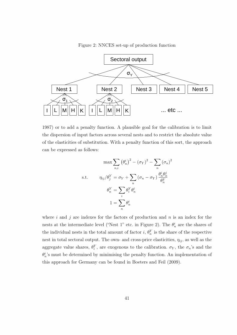
Figure 2: NNCES set-up of production function

Sectoral output

I L M H K

Nest 1

σ1

I L M H K

Nest 2

σ2

Nest 3 Nest 4 Nest 5

... etc ...

σY

1987) or to add a penalty function. A plausible goal for the calibration is to limitthe dispersion of input factors across several nests and to restrict the absolute valueof the elasticities of substitution. With a penalty function of this sort, the approachcan be expressed as follows:

max∑n,i

(θi

n

)2 − (σY )2 −∑

n

(σn)2

s.t. ηij/θYj = σY +

∑n

(σn − σY )θi

nθjn

θYn

θYn =

∑i

θYi θi

n

1 =∑

n

θin

where i and j are indexes for the factors of production and n is an index for thenests at the intermediate level (“Nest 1” etc. in Figure 2). The θi

n are the shares ofthe individual nests in the total amount of factor i, θY

n is the share of the respectivenest in total sectoral output. The own- and cross-price elasticities, ηij, as well as theaggregate value shares, θY

i , are exogenous to the calibration. σY , the σn’s and theθi

n’s must be determined by minimising the penalty function. An implementation ofthis approach for Germany can be found in Boeters and Feil (2009).

41

4.2 Dimensions of labour demand heterogeneity

In this section we review the multiple dimensions of labour heterogeneity that haveled to specific labour demand categories in applied modelling. Partly, these dimen-sions overlap with those of labour supply, discussed in Section 3.2.1. However, on thelabour demand side, different aspects are relevant. In particular, it is more challen-ging to justify a particular labour split. In the following list, we report the dimensionsof labour demand heterogeneity encountered in the literature, and we check to whichextent they can be backed up with empirical estimates of labour demand elasticities.After discussing the dimensions one-by-one, we turn to additional issues that ariseonce we combine several dimensions in a single production function (Section 4.3).

Skill type

The most prominent decomposition of labour is along the skill (or qualification)dimension. The distinction of two skill types (skilled and unskilled or qualified andnon-qualified) has a long tradition in the discussion about raising wage differentialsand skill-biased technological change (see, e.g. Berman et al., 1998). This split canbe found in many CGE models, even if they do not focus on labour market issues,simply because it is implemented in the GTAP data set (Dimaranan and Narayanan,2008). With two types of labour, the simplest way of value added modelling is a one-level structure, where capital services and the two types of labour are included with asingle elasticity of substitution. An example is the GTAP model (Hertel et al., 2008),where sector-specific elasticity estimates from Jomini et al. (1994) are used. Otherpapers with a two-skills split and a similar specification are Böhringer et al. (2005)for Germany, Boccanfuso and Savard (2008) for Senegal and the global WorldScanmodel (Lejour et al., 2006).

A potential advantage of labour split into the two standard skill types (i.e. low-and high-skilled, with college degree, or a national analogue, as the demarcationline) is the availability of advanced labour demand estimations. We can draw uponan established literature on the substitution possibilities between low skilled labour,high skilled labour and capital (e.g. Griliches, 1969; Fallon and Layard, 1975; Krusellet al., 2000). However, these results are not often used for the specification of existingCGE models. Exceptions are Agénor et al. (2003), if only qualitatively, and Rojas-Romagosa (2010), who revises the value-added modelling in WorldScan.

42

Labour splits into more than two skill categories can be regularly found in ex-isting models, but they are more difficult to back up with elasticity estimates fromthe literature. Löfgren (2001) uses four skill categories, without any substitutionpossibilities (Leontief specification). Maisonnave et al. (2009) have three categories,with a Cobb-Douglas specification. Models that use an empirical specification areBoeters and Feil (2009) (with the NNCES approach described in Section 4.1) andMIMIC (Graafland et al., 2001, p.111). Interestingly, in the estimations used for thespecification of MIMIC, capital-skill complementarity is rejected for the Netherlands.

Occupation

The classification by occupation is a close substitute for skill. The choice betweenthese two options may be driven by data availability, in particular when internation-ally comparable data are needed (Boeters and van Leeuwen, 2010). In some models,occupation and skill characteristics are combined in the labour segmentation (e.g.Carneiro and Arbache, 2003; Colombo, 2008). Giesecke et al. (2011) present an am-bitious set-up for the Vietnamese economy, which cross-classifies skill (qualification)and occupation. Labour demand of firms is formulated primarily in terms of occu-pations, which, in turn, are decomposed by skill. Households, on the other hand,are primarily defined by skill and supply occupation-specific labour according to thetransformation mechanism presented in Section 3.1.5.

Full-time and part-time labour

Hutton and Ruocco (1999) are concerned with the prevalence of part-time workamong women. This motivates them to distinguish between part-time and full-timework as imperfect substitutes in production. They report no estimation results forthe elasticity of substitution between these labour types and use a Cobb-Douglasstructure in their model. There is some empirical work trying to determine thesubstitutability between workers and hours (for an overview of the earlier literature,see Hamermesh, 1993, pp. 127-134), but it has not been used in a CGE context yet.

Formal and informal labour

The distinction between formal and informal work can be found in many CGE mod-els. There are different motivations for making this explicit in a model: productiv-ity differentials between the formal and informal sector, wage differentials betweenworkers in the two sectors, and a differential treatment in taxation (see Section 5.5for a detailed discussion). Problems of labour demand modelling do, however, not

43

arise in most cases, because formal and informal labour is used in separate sectors.The question of substitutability between formal and informal work then shifts tothe substitutability between formally and informally produced goods and servicesin consumption. Only models with highly aggregated production sectors have bothformal and informal labour in the same production function. An example is MIMIC(Graafland et al., 2001, p. 110), using estimations of Baartmans et al. (1986) forcalibration.

Rural and urban labour

Similar to the formal/informal distinction, the rural/urban divide is mostly a sec-toral one, with different sectors demanding labour in the rural and urban area. Anexception is Hendy and Zaki (2010), who allow for both rural and urban labour asinput in each sector. The elasticity of substitution is chosen without reference to anempirical study.

Gender

The gender decomposition of labour in CGE models has become more widespread,driven by the rising interest in the gender dimension of inequality and the recognitionof the special role women play for economic development. The gender decompositionhas been introduced to the literature by Fontana and Wood (2000), followed byFofana et al. (2003), Fontana (2004), Colombo (2008) and Hendy and Zaki (2010).33

As with other dimensions of decomposition, the empirical foundation is a problem.Fontana and Wood (2000) do not base their specification on empirical estimations,but argue qualitatively for relatively low elasticities “to reflect the rigidity of genderroles” (p. 1179). As those roles are highly varying across countries and in many casesalso over time, it is not likely that deep substitution parameters can be identifiedthrough econometric techniques.

Ethnicity

A more recent and less common decomposition is by ethnic group, where the spe-cific delineation of groups is country specific. Maisonnave et al. (2009) use an ethnicdecomposition into African, Coloured, Indian and White in a model of the SouthAfrican economy. In the case of Israel, Flaig et al. (2011) use the ethnic/nationality

33An early predecessor is Dixon et al. (1978), who analyse the economic consequences of anexogenous increase of relative female wages.

44

categories Jewish and non-Jewish, Israeli and non-Israeli, Palestinians and foreign-ers. In both cases, the substitution elasticities are chosen ad hoc. Maisonnave et al.(2009) assume that there is no substitution possible (Leontief specification). Theelasticities in Flaig et al. (2011) have been set relative to the GTAP skilled/unskilledsubstitution elasticity, based on expert judgement.

4.3 Labour heterogeneity in several dimensions

In Section 4.2, we have presented possible dimensions of labour demand separately.Many of the papers discussed do not only deal with one dimension, but with labourheterogeneity in two or more dimensions. Once we have more than a single dimen-sion, we must think about the structure of the production function. The followingoptions have been used in the literature:

• Cross-classifying all dimensions, deleting irrelevant combinations (if necessary)and organising all categories of labour in a single CES nest. This approach hasbeen chosen by Colombo (2008), who has a 2 × 2 × 2 classification of skill,occupation (self-employed, waged workers) and gender. Carneiro and Arbache(2003) use a non-exhaustive cross-classification of formal/informal, three skilltypes, rural/urban and civil servants in a one-level nesting.

• There are is a considerable number of examples where multi-level CES struc-tures are used for different dimensions of heterogeneity. Flaig et al. (2011)combine two skill types at the upper level with ethnicity/nationality at thelower level. Hendy and Zaki (2010) use a CES production function with threelevels: urban and rural workers at the upper level, male and female work at theintermediate level, and skilled and unskilled labour at the lowest level. Maison-nave et al. (2009) decompose three skill types at the upper level (Cobb-Douglasspecification), and four ethnicities at the lower level (Leontief specification).The dimensions in Dixon and Rimmer, 2003 are occupation and two aspectsof entitlement in a low-wage policy proposal, and in Dixon et al. (2011) occu-pation, legal status and place of birth.

Apart from the problem of finding labour demand parameters at all (in most ofthe studies reviewed, elasticities of substitution are merely guessed), with several

45

dimensions of heterogeneity, we are faced with the problem of the nesting hierarchy.Which types of labour should be grouped into a nest at a higher level, and whichat a lower level? Traditionally, a loose convention has established that factors ofproduction that are close complements are grouped together at a low level of thenesting, whereas factors that are good substitutes are combined at a higher level(i.e. higher levels of the nesting have higher values of the elasticity of substitutionthan lower levels). There is no empirical reason for such a convention. Ultimately,the only criterion that counts is which nesting fits the data best. In the case ofKLEM estimations, there have been studies that compare different CES nestingswith regard to their empirical performance (e.g. van der Werf, 2008). We do notknow, however, of any comparable study in the field of labour demand estimations.Here, the estimation techniques are rather dominated by flexible functions, whichare a candidate for direct implementation in CGE models (see Section 4.1).34

When deciding for a multi-layer CES structure, modellers are left with the ques-tion of how to set up the nesting. Let us take an optimistic case and assume that someestimates (or guesstimates) of elasticities of substitution between different varietiesin each dimension are available. It is important to realise that the same elasticitiesof substitution, if implemented in a different nesting structure, can lead to differentdemand elasticities. In a two-level nesting structure as in Figure 3, the own-priceelasticity of factor of production i is

ηxipi= −σI (1− θiI)− σ (θiI − θi) , (13)

where σ and σI are the elasticities of substitution at the upper and lower level,respectively, θi is the value share of factor i, and θiI is the value share of factor i inits relevant sub-nest. For concreteness, let us distinguish between high/low skilledand male/female workers. The value share of high skilled work is 0.3, and withineach skill class, male and female workers have the same share of 0.5. Elasticities ofsubstitution are 0.5 between skill groups and 2 between genders. The two nestingoptions are given in Figure 3. For the own-price demand elasticity for low-skilled

34A recent example for a flexible-form labour demand estimation with several dimensions oflabour heterogeneity (skill, age and type of employment contract) is Bargain et al. (2011a).

46

Figure 3: Two-level nesting options

Labour aggregate

Male 0.5

Female 0.5

High skilled 0.3 σI=2

Low skilled 0.7

σ = 0.5

Male 0.5

Female 0.5

σI=2

Labour aggregate

High 0.3

Low 0.7

Male 0.5

Female 0.5

σ = 2

High 0.3

Low 0.7

σI=0.5 σI=0.5

male work, we obtain

ηLM = −2× (1− 0.5)− 0.5× (0.5− 0.35) = −1.075

ηLM = −0.5× (1− 0.7)− 2× (0.7− 0.35) = −0.85

for the left and right panel of Figure 3 respectively. This is a significant difference.

This is another example of the general phenomenon discussed in Section 4.1:There is no one-to-one relationship between elasticities of substitution and elasti-cities of demand. We need to answer the question of which of these parameters –elasticities of substitution or elasticities of demand – we want to consider as morefundamental. General equilibrium economists tend to focus on the elasticities ofsubstitution. Researchers working on the substitution possibilities between capital,high and low skilled labour (e.g. Krusell et al., 2000) have tried to identify therelevant elasticities of substitution, not elasticities of factor demand. On the otherhand, labour market economists are often interested in labour demand elasticitiesas an ingredient to a partial labour market model (see Peichl and Siegloch, 2010). Inprinciple, this question of which elasticity is more fundamental could be approachedempirically. What is needed are comparative labour demand estimations with dif-ferent data sets (implying varying value shares). This would allow us to address thequestion: Which estimated parameters are more stable across data sets, elasticitiesof substitution or demand elasticities? However, we do not know of any empiricalstudy approaching the issue from this angle.

In the absence of an empirical guideline, we tend to favour elasticities of demandas the more fundamental ones. After all, demand elasticities are the elasticities thatare most directly linked to empirically relevant results (e.g. “By how much must

47

the wage fall to induce absorption of a certain change in labour supply?”). This is apoint in favour of treating labour demand elasticities as fundamental and calibratingelasticities of substitution (conditional on the given value shares) so that the demandelasticities are met (as in Section 4.1 in the case of the NNCES function).

5 Labour market coordination

5.1 Scope of the market

Determining the scope of a labour market in a CGE model, i.e. delineating the indi-viduals under a uniform labour market regime, touches upon a number of issues thatare hardly ever explicitly discussed in economics texts. This is because they tend tofall in-between the major fields of theoretical and empirical work. In theory papers,it is customary to merely postulate how many and which markets are to be distin-guished. Empirical labour market economists, in contrast, take multi-dimensionalheterogeneity at face value. This becomes apparent in multiple regression analysis,the very point of which is to filter out the effects of as many dimensions of het-erogeneity as possible. The question of how to delineate labour markets does notarise naturally in either the purely theoretical or the purely empirical context. Inapplied modelling, however, this question imposes itself on the model builder. It isoften answered in an implicit way, which remains silent about other options andabout the consequences of a particular choice. In this section, we want to make therelevant issues more explicit.

By the criteria reviewed in Sections 3 and 4, both labour supply and labour de-mand are potentially differentiated in several dimensions. The follow-up question isabout whether, and to which extent, this differentiation is to be transferred to labourmarket coordination. There are two extreme options to decide this question: (1) alarge number of very narrowly defined labour markets with an independent wagerate in each of them, or (2) a single labour market, in which the sum of all supplyand demand is coordinated. In practical modelling, labour market differentiation ismost often driven by the supply rather than the demand side. Model builders aremotivated, either by distributional concerns or by the design of the policy instru-ment, to distinguish between different types of workers (e.g. by gender, age or skill

48

level) and impose this distinction on labour demand and labour market coordinationas well.

It is a basic point to be kept in mind, however, that we do not have to differenti-ate between labour markets simply because we have decided to distinguish betweendifferent types of labour. Treating different types of labour as homogeneous inputsand aggregating them in a single market with a uniform wage is a perfectly viableoption. Naturally, wage differentials between individuals are an empirical fact, whichis, prima facie, not compatible with a homogeneous market. However, there are atleast two simple mechanisms – both discussed in a CGE context by Boadway andTreddenick (1978) already – that allow us to work with a uniform market model inspite of existing wage differentials. The first of these mechanisms is efficiency weight-ing. Individuals with higher hourly wages are assumed to supply more effective unitsof labour per hour than low-wage individuals. Weighting with individual-specific ef-ficiency factors derived from the wages, we can simply add up labour supply ofheterogeneous individuals. Assuming efficiency factors to be constant implies thatwages of different individuals in one market move precisely in proportion, leavingrelative wages unchanged.

The second mechanism for accommodating wage differences without separatingmarkets are compensating wage differentials, typically applied to sectoral wages.Jobs in different sectors are associated with varying non-pecuniary conditions suchas riskiness of the job or agreeableness of the work sphere. Under inter-sectoralmobility of workers, differences in observed wages can be rationalised by assumingthat lower wages are compensated by non-pecuniary benefits so that, taken as apackage, job opportunities are equally attractive for workers across sectors.35 Simpleand well-established as this idea is, it may create follow-up problems in modelling:(1) Non-pecuniary benefits contribute to household utility and must be accountedfor when performing a welfare analysis. (2) As a contribution to household utility,non-pecuniary benefits might have an income effect on labour supply.36 (3) If there

35It is a considerable empirical challenge in itself to determine what share of observed sectoralwage differentials is attributable to a different composition of the work force, and what shareremains as a pure sectoral wage differential. It has repeatedly been shown that neither of theseshares is negligible (see, e.g. Slichter, 1950; Krueger and Summers, 1988; Genre et al., 2011).

36In Böhringer et al. (2005) this effect is included in the following way: Labour supply responds,

49

is involuntary unemployment, this is an additional factor contributing to the relativeattractiveness of sectors, see Section 5.5.37

The crucial empirical question for labour market differentiation is whether wagesof different groups of workers move in parallel (with appropriate constant adjustmentfactors) or not. This question arises almost exclusively in the modelling context, oncewe want to determine whether market segmentation is appropriate or not. So it is nosurprise that it has not been addressed in existing empirical labour market studies,with the exception of the wage differential between skilled and unskilled workers. Forother potential labour market segmentations original empirical research is required.A case in point is gender-specific labour markets. There is a growing literatureinterested in gender-specific labour-market consequences of various policy shocks(e.g. Fontana and Wood, 2000, Fofana et al., 2003, Hendy and Zaki, 2010). Thesestudies assume that there are separated labour markets for men an women, butthey do not provide empirical evidence supporting an independent movement ofgender-specific wages. If such evidence exists, it could considerably strengthen themodelling set-up.

Another basic point to be kept in mind is that homogenising forces on one side ofthe market, either supply or demand, are sufficient for the constitution of a homogen-eous labour market. If labour is perfectly transformable between different categories(see Section 3.1.5), this will create a uniform labour market, because any poten-tial wage differential would provoke labour supply adjustments that cause wages toequalise. The most relevant case is sectoral labour mobility. In almost all other di-mensions of labour supply heterogeneity (gender, age, skill), transformation optionsare limited, if existent at all. – The mirror image of a labour-market homogenisingeffect can arise at the labour demand side. Once two types of labour are perfectlysubstitutable in production, any difference in the wages will disappear. While it isstandard in labour demand modelling to assume imperfect substitutability of skill

not to the wage per se, but to the value of a job. The value of a job, in turn, is equal across sectorsand composed of three components: wage, non-pecuniary benefits and unemployment risk.

37The approach of Devarajan and Rodrik (1991) remains somewhere half-way in this compensat-ing differential story. They assume sector-specific efficiency factors which are calibrated to matchintersectoral wage differentials. However, they do not address the question of what prevents allworkers from switching to the highest paying sector.

50

types, the case with other dimensions of labour heterogeneity (gender, age, hours ofwork) is much more complex. Clearly, the burden of proof is with those that claimimperfect transformability in these cases (see Section 4.2).

A special constellation to be mentioned is one-way transformation or substi-tution, which causes asymmetry between labour market segments. An example isthe dual labour market model of Harris and Todaro (1970), discussed in Section5.5, where workers who do not find a job in the formal sector can always retreat tothe informal sector, but not in the opposite direction. Another asymmetry pattern isplausible in the demand for skills. There are many low-skilled tasks that can withouta problem be taken over by high-skilled workers, if necessary – but not inversely.

5.2 Wage forming mechanism

The vast majority of CGE models have worked with one or both of the two extremeassumptions about wage formation: flexible, market clearing wages and institution-ally fixed wages. In the market-clearing set-up, competition on both sides of thelabour market is assumed so that wages equilibrate demand and supply and there isno involuntary unemployment. In contrast, in the fixed-wages set-up, wages do notrespond to changes in supply or demand conditions. Labour supply and demand aredetermined given a fixed level of wages, and the resulting difference is interpretedas involuntary unemployment.

Simple as it seems, the fixed-wages set-up is not without difficulties in a CGEcontext. Actual wage contracts are usually fixed in nominal terms. In general, how-ever, nominal prices are undetermined in CGE models, since only relative priceshave significance. If we nevertheless fix a nominal wage in our CGE model, whatwe essentially do is fixing a real wage in terms of the numéraire of the model.38 Weconsider it to be good modelling practice to make the fixation of real wages explicitand not implicit through the choice of a numéraire.39 If the domestic consumer priceindex (CPI) is chosen to be the numéraire, the fixation of nominal wages may well

38We have come across CGE papers where the authors apparently confused fixing the wage asan institutional feature of the labour market and using it as the numéraire of the model.

39The numéraire choice is often not reported in the model description, just because it is assumedto be arbitrary. In this case the fixation of nominal wages becomes a black-box phenomenon.

51

be plausible, because explicit or implicit indexation of wages to consumer pricesis a common phenomenon.40 However, it is not in all cases that the CPI acts asnuméraire. In many applied one-country models of small open economies this roleis taken by the export and import prices. Then fixing a nominal wage means thatthe wage is indexed to foreign prices, which is implausible, except if it is an explicitinstitutional feature of the economy modelled.

Fixing real wages is the simplest possible way of accounting for labour marketrigidities and involuntary unemployment. However, being simple means being re-strictive as well. Even if we take it for granted that there are institutions fixing thereal wage, this fixation will hardly be absolute. At least in the medium and long run,wages do adjust to labour market conditions, even if subject to longer lasting con-tracts. So the next plausible step is to think about which labour market conditionswill drive the wage adjustment and how the adjustment takes place.

In general, any in-between modelling of labour market rigidities will have theform of a “wage curve”. Understood in a broad sense, this is any locus off the laboursupply curve whose intersection with labour demand determines the wage, thusreplacing labour supply in this function. There are two principal approaches tothe construction of a wage curve. The first one is empirical. We start from theobserved situation and try to determine the factors driving changes in the wageeconometrically. The result of the estimation is then implemented as an empiricalwage curve in the model (for an overview, see Folmer, 2009). The “Wage Curve”(in a narrow sense) of Blanchflower and Oswald (1995) is the best known exampleof this approach. Blanchflower and Oswald find an empirically astonishingly stablerelationship between the level of unemployment and the wage (see our extensivediscussion in Section 5.6). Two examples of models that include the unemployment-wage relationship (and only this) explicitly as one of the equations are Hutton andRuocco (1999) and Maisonnave et al. (2009). In the MIMIC model (Graafland et al.,2001, p. 125), the wage depends, in addition, on the average and marginal labourtax rates.

For setting up a wage curve to be empirically estimated, we need to determine

40This is explicit, for example, in Dixon et al. (1978), Corden and Dixon (1980), Dixon et al.(1982).

52

the variables that are candidates for inclusion in the equation. Usually, this is donebased on a structural model of wage determination in imperfectly competitive labourmarkets, which brings us to the second approach to the wage curve. There arethree theories that have been used in this way: search and matching (Pissarides,1990), efficiency wages (Shapiro and Stiglitz, 1984) and collective wage bargaining(McDonald and Solow, 1981). By establishing a wage that is above the market-clearing level, these theories cover at the same time the phenomenon of involuntaryunemployment. As theories of unemployment they are discussed in the followingsection (5.3).

The attempts to determine the empirical content of these structural theories ofwage formation may be classified into two strands. In the first, dominant type ofliterature, the theories are used to derive empirical wage curve specifications, whichare then used to generate elasticity estimates (as reviewed in Folmer, 2009). In thesecond type of literature (Pissarides, 1998, and Sørensen, 1999), the focus is onthe structural parameters in each of the theories. These are identified and givenempirically plausible values. Our review in Section 5.3 follows the second approachand pays particular attention to the question of how this fits in with the stylisedfact of Blanchflower and Oswald’s wage curve.

5.3 Involuntary unemployment

Pissarides (1998) and Sørensen (1999) show how the most prominent options ofmodelling unemployment – search and matching, efficiency wages and collectivebargaining – are calibrated and implemented in a simple CGE context. We start bybriefly reviewing the core ideas of the three options, before going into more detailin Sections 5.3.1 to 5.3.3.

The search-and-matching model starts from the core assumption that finding ajob is a time- and effort-consuming process, the more so, the less vacancies thereare. Similarly, posting a vacancy is costly, and not worth the effort if there areno unemployed workers to be found. Therefore a certain level of unemployment isnecessary to keep the process of continuous reallocation of jobs running. The levelof unemployment is determined by structural parameters of the labour market, suchas the efficiency of the matching process.

53

Search-and-matching models exist in a vast number of varieties, which is partlydue to the fact that they lend themselves conveniently to empirical estimation withmicro data. The model varieties differ in several aspects: whether there is on-the-jobsearch or not, how wages are determined once a match materialises, and whetherjobs and/or workers are homogeneous or heterogeneous in productivity. However,only the most simple of these varieties have been used in a CGE context.

The core idea of the efficiency wage model is that employers can increase theproductivity of workers by paying wages that are above the market-clearing level.There are several versions of the precise productivity-increasing mechanism. In theoriginal version the market-clearing wage is below the subsistence level of workers sothat only higher wages allow workers to reproduce their working skills (Leibenstein,1963). In other versions of the story higher wages increase the motivation of workers(“gift exchange”, Akerlof, 1982), or they create unemployment so that firing workersbecomes a serious threat that deters workers from shirking (“unemployment as aworker disciplining device”, Shapiro and Stiglitz, 1984). In any case, the formaltheory starts from an efficiency curve, which gives work efficiency as a function ofthe (relative) wage. For the empirical implementation, the story behind this efficiencycurve is not strictly necessary.

The collective wage bargaining model formalises the idea that wages result fromnegotiations between firms’ associations and trade unions. The crucial idea is thatpart of the social costs of higher wages and resulting unemployment are externalitiesnot borne by the bargaining parties in a particular sector, but by society as a whole(through unemployment benefits financed by general tax revenue or social securitycontributions). This externality induces the bargaining parties to go for wages thatare above the market-clearing level.

In the case of bargaining theories, as well, we have quite a few sub-varieties:right-to-manage versus efficient bargaining, insider model versus utilitarian union,bargaining over wages only versus bargaining over wage/hours-of-work packages,monopoly union versus two bargaining parties. However, the differences betweenthese varieties become small, or even irrelevant, once the model is calibrated to theactual unemployment rate. For the case of the insider model versus utilitarian unionmodel this is shown in Boeters (2011).

54

Even if we tend to use a structural model for the implementation of involuntaryunemployment, we are left with the difficult question of which one to use. All mech-anisms sketched above have their plausibility, albeit to a different degree in differentsegments of the labour market. The search-and-matching mechanism is certainly animportant element in any convincing explanation of unemployment. But one candoubt whether this is the whole story. It characterises unemployment mainly as atransitory phenomenon and downplays long-term, structural effects. The efficiency-wage approach is right in stressing the disciplining effect of unemployment, but onecan doubt whether work effort would actually drop to zero without unemployment,as the shirking theory implies. Finally, the relevance of collective bargaining forwage formation is mainly determined by the concrete institutions of the country inquestion. It is considerably higher for continental Europe and Scandinavia than forthe Anglo-Saxon countries.

In the following paragraphs, we present simple formalisations of the three ba-sic approaches. We also discuss how, and to what extent, they can be given anempirically meaningful interpretation in a CGE context.

5.3.1 Search and matching

The core element of any search-and-matching model is the matching function, whichgives matches, M , as a function of the number of unemployed workers, U , andvacancies, V . A Cobb-Douglas specification with efficiency parameter µ and shareparameter ε (0 < ε < 1) reads:41

M = µU εV 1−ε

It is convenient to define “labour market tightness”, θ, as an additional variable:

θ ≡ V/U

and express the probabilities of finding a job, a, and filling a vacancy, q, as

a ≡ M/U = µθ1−ε

41The material of this section follows closely the expositions in Pissarides (1998) and Sørensen(1999).

55

q ≡ M/V = µθ−ε

There are two different labour market states for workers: employed (index E) andunemployed (index U). With instantaneous utilities U , discount rate ρ and exogen-ous separation rate s for existing jobs, the following recursive value equations canbe formulated, where J i is the value of being in state i.

ρJE = UE − s(JE − JU

)ρJU = UU + a

(JE − JU

)Analogously, on the part of the firm, jobs can be either occupied (index O) or vacant(index V ). With job productivity42 p, labour cost w and vacancy cost γ, we have

ρJO = p− w − s(JO − JV

)ρJV = −γ + q

(JO − JV

)Finding a match for a vacant job creates a rent, which needs to be shared betweenfirm and worker. A simple sharing rule is Nash bargaining, which is formalised as themaximisation of a Nash function containing the weighted product of the individualshares, JE − JU for the worker and JO − JV for the firm. In logs and with λ as therelative bargaining power of the worker, Nash bargaining can be formulated as

maxW

[λ log(JE − JU) + log(JO − JV )

]where the bargaining parties treat JU and JV as exogenous. This gives the followingfirst order condition:

λdUE

dw

(JO − JV

)−(JE − JU

)= 0

Substitution of the state value variables, observing the free-entry condition, JV = 0,brings us to

dUE

dwλγ (ρ + s + a)− q

(UE − UU

)= 0

If utility is linear in consumption, we have

dUE

dw= 1− tm

42Productivity is endogenous in a general equilibrium context, but it remains exogenous for theindividual firm.

56

UE = (1− ta) w

UU = c (1− ta) w

where tm and ta are the marginal and average tax rates on labour income, and c isthe replacement rate (unemployment benefit as a share of after-tax labour income).Then we have

(1− tm) λγ (ρ + s + a)− q (1− c) (1− ta) w = 0

and w can be expressed as a mark-up on the cost of a vacancy, γ.

w =(1− tm) λ (ρ + s + a)

q (1− c) (1− ta)γ (14)

As long as the institutional parameters – λ, c and the tax rates – are constant,the mark-up factor depends positively on the probability of finding a job, a, andnegatively on the probability of filling a vacancy, q. In the dynamic equilibrium,43

inflow to and outflow from unemployment must be the same, which means

au = s(1− u)

and can be used for replacing a in eq. (15):

w =(1− tm) λ

(ρ + s

u

)q (1− c) (1− ta)

γ (15)

This is a wage curve in the narrow sense, because it gives us the wage, w, as adecreasing function of the unemployment rate, u.

Calibration

The calibration of the search-and-matching model to empirical wage curve elasticit-ies turns out to be a problem. Taking logs on eq. (15) and calculating the partialderivative with respect to u gives the wage curve elasticity

ηwu =d log w

d log u= − s

uρ + s(16)

The expression on the right hand side contains only three parameters, the separa-tion, unemployment and discount rates. These are parameters on which in principle

43We focus on the equilibrium version of the search-and-matching theory. An interesting disequi-librium set-up, whose ambition is to cover short-term adjustment as well, is presented in Dixonand Rimmer (2003) and applied to illegal immigration in Dixon et al. (2011).

57

empirical information is available. In contrast, parameters that are difficult to fix em-pirically, namely the bargaining power λ and the vacancy cost γ, have disappeared.Rather than helping us to determine additional parameters, eq. (16) produces anempirical implausibility. At a yearly basis,44 s is of the same order of magnitude asu, and ρ is small. This gives a value of close to −1 for eq. (16), considerably divergingfrom the prominent Wage Curve elasticity value of −0.1. (See Section 5.6 for theinterpretation of empirical Wage Curve estimates.)

This empirical implausibility is not necessarily the end of the calibration story.It is reasonable to argue that in eq. (15), the probability of filling a vacancy, q, is notto be treated as a parameter, but as an endogenous variable that moves inverselywith unemployment. However, deriving the precise functional relationship is notstraightforward and involves other equations, which again requires decisions aboutwhat is endogenous and what is exogenous.

5.3.2 Efficiency wages

The cornerstone of the efficiency wage theory is some kind of monitoring technology,which is necessary in order to enforce discipline among the workers.45 In the simplestcase we have discrete effort, i.e. workers decide whether to exert either no effort or agiven effort package, which avoids being detected shirking. The detection technologyis monitoring in regular time intervals, which uncovers shirking, if present, withprobability q. As in the search-and-matching set-up, we work with recursive valuefunctions. This time we have three, for employed workers that shirk (index ES) ordo not shirk (EN), and for the unemployed (U ):

ρJEN = UEN − s(JEN − JU

)ρJES = UES − (s + q)

(JES − JU

)

ρJU = UU + a(JE − JU

)44The choice of the time unit for flow accounting is relevant to the individual flow rates. However,

changing the time unit would affect s and ρ proportionally so that the effect cancels out.45The following formulation of the theory is based on Pissarides (1998), who in turn draws upon

Shapiro and Stiglitz (1984).

58

where the J are state values, U are instantaneous utilities, s is the exogenous sep-aration rate, ρ is the discount rate, and a is the probability of finding a job. In thesteady state, where the flow equilibrium must hold, a can be expressed in terms ofthe unemployment rate, u,

a =s (1− u)

u

If they want to prevent shirking, firms must offer a wage that makes workers indif-ferent between shirking and not shirking, i.e.

JEN = JES = JE (17)

For tracing out the algebraic consequences of this, we must specify the instantaneousutility function. A common specification (e.g. Pissarides, 1998) is to assume linearityin the wage and commensurability of effort, e, with the wage so that we have

UEN = w − e, UES = w UU = b

with unemployment benefits b. Then the non-shirking requirement (17) results inthe wage equation

w = ρJU +ρ + s + q

qe

i.e. the wage is determined as a mark-up on the annualised value of unemployment,which increases with the required effort, e, and decreases with the detection prob-ability, q. Further substitution of JU leads to

w = b +[ s

u+ ρ + q

] e

q(18)

If unemployment benefits are defined as a fixed share of the wage (i.e. we have aconstant replacement rate, c), we can use b = cw, and eq. (18) turns into

w =1

1− c

[ s

u+ ρ + q

] e

q(19)

Calibration

Eqs. (18) and (19) are wage curves in the strict sense that they contain a negativeeffect of the unemployment rate, u, on the wage, w. In the calibration context, wehave good prospects to obtain information on (or estimation of) the separation rate,s, the discount rate, ρ, the unemployment rate, u, and the replacement rate. Two

59

unknowns remain, e and q, for which there are no prospects of empirical foundation.46

As eq. (19) must hold in equilibrium,47 we can formulate an expression for e as afunction of q:

e = (1− c) q( s

u+ ρ + q

)−1

(20)

where e is the effort normalised by the wage, e = e/w.

From eqs. (18) and (19), we can calculate the respective wage curve elasticities,ηwu and ηc

wu.

ηwu =d log w

d log u= − se

qu(21)

ηcwu = − 1

1− c

se

qu(22)

Using eqs. (20) and (21) to eliminate e, we arrive at

q = − s

u

(1− c

ηwu

+ 1

)− ρ (23)

q = − s

u

(1

ηcwu

+ 1

)− ρ (24)

This allows us to calculate q. If we choose plausible values for the other parametersin eq. (23), s = 0.2, u = 0.1, c = 0.6, ρ = 0.05 and the target wage curve elasticity ofηwu = −0.1, then we end up with q being close to 6. In the case of a fixed replacementrate, this increases to close to 18. Interpreting these values, it is important not tointerpret q as a probability (where values above one do not make sense), but as aninstantaneous probability rate. A rate of above one means that the relevant event(caught while shirking) is expected more than once in the time interval (one year).Values of 6 and 18 for q then mean that a shirker is caught roughly after 2 monthsand in less than one month respectively. 48

46The calibration of the efficiency wage model, again, closely follows Pissarides (1998).47(19) must hold in both cases, even if unemployment benefits are not defined as a fixed share

of the wage.48Pissarides (1998) observes the problem of the indeterminacy of q and e as well. He does not

resort to the wage curve for calibration, however. Instead, he uses arguments based on the valueof leisure time in the utility function. This produces a consistency problem, because in his modelspecification, utility is linear in income, as in the model of this section.

60

5.3.3 Collective wage bargaining

In the model discussed in this section, wage formation is conceptualised as the out-come of collective bargaining between a trade union and a representative firm. Thereare many varieties of this model, but for a concrete start, and to establish terms, wemake more specific assumptions: (i) bargaining is only about the wage, not aboutemployment (“right-to-manage” approach)49, (ii) the trade union is only concernedwith the utility of its employed members (“insider model”)50, (iii) hours of workare exogenous. Formally, wage determination is implemented as the maximisationof a Nash bargaining function, Ω, where trade unions are represented by the utilitymark-up over their fallback option, Ue−Ua, and firms by profits, π. The relative bar-gaining power of the trade union, λ, is an unobservable parameter to be determinedin the calibration.

maxw

Ω = (Ue − Ua)λ π (25)

Maximisation is with respect to the before-tax wage, w.51 The fallback option of theunion, Ua, is composed of possible employment in another sector, Ue, and unem-ployment (receiving unemployment benefits), Uu, with weights determined by theunemployment rate, u:

Ua = (1− u)Ue + uUu

The fallback option is exogenous to the individual wage bargain so that the first-order condition of the maximisation of the Nash function is

λdUe/dw

Ue − Ua

+dπ/dw

π= 0

Both firms and employed workers make optimal choices, given the wage. This allowsus to apply the envelope theorem and express the first-order condition in terms of

49Sørensen (1999) shows that for the type of numerical analysis intended, the choice betweenright-to-manage and efficient bargaining (where bargaining extends also to the number of employedworkers) hardly matters.

50Further below in this section, we show that the results are identical to those obtained with autilitarian union as long as the value shares and the elasticities of labour demand and hours supplyare constant.

51Maximisation with respect to the after-tax wage yields the same results. Nevertheless, thedistinction must be kept in mind when comparing the formulas obtained with the literature.

61

partial effects:

λ∂Ue/∂w

Ue − Ua

+∂π/∂w

π= 0

where the partial effect for the firm under profit maximisation is

∂π

∂w= −L

Finally, using elasticities, we have

∂ log Ω

∂ log w= λ

∂ log Ue

∂ log w

Ue

Ue − Ua

− wL

π= 0. (26)

General equilibrium

With symmetrical sectors in equilibrium, we set

Ue = Ue

and eq. (26) can be re-formulated as

∂ log Ω

∂ log w= λ

∂ log Ue

∂ log w

Ue

u (Ue − Uu)− wL

π= 0.

This reveals the basic wage curve relation: The higher unemployment, u, the lowerthe union benefit from a marginal increase of w, and, consequently, the lower thewage in equilibrium.52

Calibrating the bargaining power parameter

The relative bargaining power of the trade union is a parameter notoriously im-possible to observe. Its value can be recovered, however, from the observed unem-ployment rate. Assuming that the initial state is an equilibrium, eq. (26) must holdand the value of λ can be determined as53

λ =wL

π

(∂ log Ue

∂ log w

)−1u(Ue − Uu

)Ue

(27)

The value of λ depends on the specification of the utility function. In particular, itdepends on the modelling of the utility of the unemployed, i.e. how a difference inincome compared to the employed translates into a difference in utility (see Section

52See our general discussion of the wage curve as basis for calibration in Section 5.6.53Variables with an upper bar denote the values of the initial equilibrium used for calibration,

and are therefore treated as constant.

62

3.1.4). However, given a particular specification of the utility function, the calcula-tion of λ is straightforward.

The numerical essence of the Nash bargaining first-order condition can then beexpressed as

∂ log Ue

∂ log w

Ue

Ue − Ua

=wL

λπ:= ζ (28)

If we are prepared to assume that we are in a Cobb-Douglas world (or close toit),54 then ζ is a constant, and the Nash FOC boils down to keeping the left-handside of eq. (28) at its initial level. This does not change when we work with otherspecifications of the trade union’s objective function.

In the case of a utilitarian union, which also takes the level of employment intoaccount when bargaining over the wage, the Nash function is

Ω′ = [(Ue − Ua)L]λ π,

and the corresponding first-order condition

∂ log Ω′

∂ log w= λ

(∂ log Ue

∂ log w

Ue

Ue − Ua

− εLw

)− wL

π= 0, (29)

where the additional term, εLw is the (absolute value of the) elasticity of employment,L, with respect to the wage.

εLw = −∂ log L

∂ log w

As long as this is constant or almost constant, we are essentially back at eq. (28),although λ has a different value now.

λ′ =wL

π

((∂ log Ue

∂ log w

)Ue

u(Ue − Uu

) − εLw

)−1

.

Compared to eq. (27), the denominator shrinks, and thus λ′ > λ. A utilitarian unionis roughly equivalent to an insider union that has a (correspondingly) lower relativebargaining power.

54The assumption can be formulated still somewhat weaker: Even if the factor shares change, thiswill not have a systematic effect on wage negotiations. This comes close to denying the assumption,implicit in the Nash bargaining function, that parties bargain over relative mark-ups over theirrespective outcome. So if some shock increases (reduces) the basis they bargain upon, their mark-upwill increase (fall) accordingly. This mechanism does not have much intuitive appeal.

63

The same applies to a more general Nash function with variable weights forindividual utility and employment, such as

maxw

Ω′′ = (Ue − Ua)λLµπ,

which includes both the utilitarian union (λ = µ = 1) and the insider model ofeq. (25) with λ = 1 and µ = 0 (see Graafland et al. 2001, ch. 7).

∂ log Ω′′

∂ log w=

(λ

∂ log Ue

∂ log w

Ue

Ue − Ua

− µεLw

)− wL

π= 0, (30)

This leaves us with two parameters, µ and λ, which cannot be identified through asingle first-order condition without further information. However, we can choose anarbitrary value of µ, solve for λ, and – as long as the value shares and the labourdemand elasticities are constant – we still remain with the essential equation

∂ log Ue

∂ log w

Ue

Ue − Ua

=

(∂ log Ue

∂ log w

)Ue

u(Ue − Uu

)Linear utility function

The majority of the existing literature works with the simplifying assumption of autility function that is linear in net income. If individual hours of work are exogenousand normalised to unity, we have

Ue = (1− ta)w

Uu = b

where b are unemployment benefits. We then can solve the first order conditions ofNash bargaining explicitly for the wage, which gives us a wage curve

w =ζu

ζu(1− ta)− (1− tm)b (31)

where w is increasing in ta and b, and decreasing in u and tm.

The picture is different if we assume that b is not given in absolute terms but asa constant share (“replacement rate”) of after-tax income:

b = c(1− ta)w

64

Then w drops out of the wage-bargaining first-order condition and we are left with

1 =ζuc(1− ta)

ζu(1− ta)− (1− tm)

This can be solved for u

u =(1− tm)

ζ(1− ta)(1− c)(32)

u is increasing in c and ta, and decreasing in tm. We now have an explicit expressionfor u, but the downside is that w cannot be determined from the first-order conditionany more but only in general equilibrium. With exogenous labour supply55 N , em-ployment is determined as (1−u)N , and w results implicitly determined as the wagethat – given macroeconomic labour demand – creates the desired employment level.There is a monotonous relationship between u and w, but without knowing generalequilibrium elasticities, we cannot say anything about the wage curve elasticity.

Empirical implications

Again, we look at two extreme cases: unemployment benefit fixed in real terms anda constant replacement rate. In the case of fixed unemployment benefits, we havean explicit wage curve, eq. (31), which allows us to calculate the implied wage curveelasticity. With proportional taxes (ta = tm) this is

ηwu = − 1

ζu− 1

Taking into consideration the calibration of ζ, eq. (28), and assuming a Cobb-Douglasworld, where factor shares are constant, we arrive at

ηwu = −1− c

c

For a replacement rate of c = 0.6, this means a wage curve elasticity of ηwu = −0.67,which is considerably higher than the empirically plausible value of −0.1.

In the case of a fixed replacement rate, we have the unemployment rate as afunction of policy parameters:

u =(1− tm)

ζ(1− ta)(1− c)

55When labour supply is endogenous, even more equations become relevant to the determinationof the wage.

65

i.e. the wage moves independently of u, which makes the derivation of a wage curveelasticity impossible.

The challenge in calibrating the wage curve of the collective bargaining modelis finding a specification that leaves enough flexibility for adjustment to empiricalparameters. A possible approach is to define a “mixed replacement rate regime”,in which unemployment benefits are a linear combination of a fixed part and anindexed part. With α as the share of the fixed part, we have

b = αb + (1− α)cw

resulting in a wage curve

w =αζu

ζu(1− ta)− (1− tm)− (1− α)cζub

The same substitutions as above, combined with the assumption of a proportionaltax schedule, yield the wage curve elasticity

ηwu = −(1− t)(1− c)

(α− t)c

For α = 1, this reproduces the elasticity value ηwu = −(1 − c)/c derived earlier.Other values for α lead to a shift in ηwu. However, as one is the upper bound for α,changing α can only increase the (absolute value of the) wage curve elasticity, anddoes therefore not solve the calibration puzzle.

5.4 Long-term trends in unemployment

In the dynamic calibration of unemployment, we are faced with a problem similar tothose discussed in the context of labour supply (see Section 3.5). A secular upwardstrend in labour productivity, and thus in wages, can produce a trend in unemploy-ment, which might well be spurious. This is because the comparison of state valuesfor employment and unemployment, and essentially the instant utility values forthese two states, are crucial for all structural models of unemployment. If an up-ward trend in wages changes the relative values of employment and unemployment,this will have a systematic effect on unemployment.

With unemployment benefits determined as a fixed share of the after-tax incomeof the employed (constant replacement rate), and utility linear in income, we arrive

66

at a benchmark situation in which the unemployment rate remains constant even ifwages change. Comparison with this reference case reveals how a trend in wages cansystematically influence unemployment. When unemployment benefits are fixed inabsolute terms and do not evolve proportionally with wages, wage increases makeemployment more attractive compared to unemployment, and thereby reduce theunemployment rate. The inverse effect occurs when we combine a constant replace-ment rate with basic, non-utility-generating, consumption, e.g. in a linear expendit-ure scheme. A proportional development in income for the employed and unemployedthen does not translate into a proportional development of utility any more. Withbasic consumption uniform for both groups, relative utility of the unemployed willincrease with rising wages, generating an upward trend in unemployment.

Similar non-proportionality effects may be produced by leisure as a utility-generating item (see Sections 3.1.1 and 3.1.4) or by adjustment factors for leisureproductivity (see Section 3.5). In the collective bargaining model (see Section 5.3.3),we have a simple option for neutralising all these systematic effects on unemploymentin the long run. λ, the relative bargaining power of trade unions, may be treated as atime-varying parameter, adjusted so that unemployment remains constant over timein the baseline. In the search-and-matching and efficiency wage models, the match-ing efficiency and the parameters of the monitoring function can take on similarroles for calibration.

5.5 Informal sector and dual labour market

In this chapter, we have repeatedly touched upon the issue of an informal sectorand the “dual labour market” structure it can give rise to. For distributional andpoverty analysis in particular, the distinction between the formal and informal sectoris indispensable, given that a large fraction of the poorest workers are located inthe latter (Fortin et al., 1997). Here we collect different aspects of this issue andinvestigate whether the dual labour market structure can be seen as simply onespecial case of differentiated labour markets (as discussed in Section 5.1).

On the labour demand side, it is usually a sectoral distinction that motivatesthe formal/informal divide. There is a number of different reasons for distinguishingbetween these two sectors: differences in technology, in wage formation or in the

67

administrative treatment of firms (in particular taxation), see Fortin et al. (1997)for an overview. A typical assumption about wage formation is that in the informalsector, wages are competitive at a full employment level, whereas in formal sector,wages are above the market-clearing level by one of the mechanisms discussed inSection 5.3 or some form of rent sharing. The basic idea of the “dual labour market”set-up of Harris and Todaro (1970) comes in on the labour supply side. Formal andinformal labour markets are not seen as completely separated (which would amountto a simple labour market segmentation as discussed in Section 5.1), but as connectedthrough imperfect labour mobility. With the wage higher in the formal than in theinformal sector, we need a rationing mechanism that prevents a complete shift ofthe workforce to the formal sector. According to Harris and Todaro (1970), thecrucial element is unemployment. Searching for a job is a time-consuming process(as highlighted in the search-and-matching literature, Section 5.3.1), therefore acritical level of unemployment will stop the migration from the informal to theformal labour market. The marginal worker is indifferent between a secure job inthe informal sector and an uncertain job search process in the formal sector (“waitingqueues” for jobs).

In the original Harris and Todaro (1970) set-up, migration between the informaland formal sectors is seen as a dynamic phenomenon, with the change in the numberof workers in the formal sector as a function of the difference between the expectedwage in the formal sector and the certain wage in the informal sector. This dynamicspecification has been implemented, e.g., in Agénor et al. (2003, Section 3.2.1). Inmost comparative static applications, however, a steady state assumption is used,to the effect that expected wages must be equal for all migration incentives todisappear,

wi = (1− u)wf (33)

where wi and wf are informal and formal wage respectively, and u is the unemploy-ment rate in the formal sector.56 Eq. (33), however, has an apparent shortcomingwhen it comes to calibration. The formal-informal wage differential as well as theunemployment rate are in principle (though not perfectly) observable, and eq. (33)will hold by mere coincidence. Only by introducing some degree of freedom can

56Harris-Todaro loci of this simplest possible form can be found, e.g., in the models of Gilbertand Wahl (2002) for China, Alzua and Ruffo (2011) for Argentina.

68

eq. (33) be changed into a form that can be calibrated. The most straightforwardway of creating this degree of freedom is to introduce fixed cost of migration (cm),which is most plausible when informal and formal sector are thought to be separatedspatially (as for example rural versus urban sector).57 Even if there is no distanceto be bridged, “fixed cost of migration” can be thought of as the cost of becomingaccustomed to the rules and conventions of the formal labour market, and of estab-lishing the contacts necessary to find a job. With fixed costs of migration in place,the Harris-Todaro locus becomes

wi + cm = (1− u)wf (34)

and cm can be calibrated so that eq. (34) holds for empirical values of unemploymentand the wage differential. In more general terms, cm can be understood as any utility-generating difference between the sectors (apart from the wage and unemployment),e.g. less flexibility or a higher status in the formal sector.58

The next hurdle for the Harris-Todaro locus to be taken is the empirical elasticityof migration. Eqs. (33) and (34) both assume that, in a partial analysis of the formalsector and as a reaction to a change in the formal wage, unemployment must adjustso that the product of the employment rate and the wage remains constant, i.e. theelasticity of unemployment with respect to the formal wage is

εuwf=

1− u

u

This can be compared to wage curve estimations and checked against expert judge-ment. If the outcome of this check is that more adjustment is needed, we have thefollowing two possible extensions. First, we can assume that the migration costsare not uniform across workers, but heterogeneous. The workers who have the low-est migration costs switch to the formal market first, so that marginal migrationcosts are increasing with the size of the formal sector, and the migration elasticity

57In many applications, the formal/informal and urban/rural distinction have been used inter-changeably. Stifel and Thorbecke (2003), however, make the point that they need to be distin-guished, which leads to a “dual-dual” model.

58Stifel and Thorbecke (2003, p. 220) encounter the same problem and solve it with some ad-hod“adjustment parameter”, used as a multiplier for unemployment in (33).

69

is reduced compared to the case with homogeneous migration costs.59 Second, wecan go beyond the simple comparison of expected wages and proceed to expectedutilities. This requires specifying the utility of the unemployed in the formal sector.Is there any unemployment compensation? If not, how do the unemployed organisethemselves to make their living? In any case, the Harris-Torado locus becomes

U(wi) = uU(wu − cm) + (1− u)U(wf − cm) (35)

By specifying the elasticity of the utility function with respect to income (which inturn determines the degree of risk aversion), we can change the migration elasticity.With no risk aversion, eq. (35) essentially collapses back into the form of eq. (34).With risk aversion, in contrast, an increase in unemployment is more detrimentalto utility than to the expected wage. Therefore, we need a smaller increase in un-employment to compensate for a given wage rise. This means that the migrationelasticity is lower than in the case of eq. (34).60

The Harris-Todaro approach is not restricted to assuming full employment inthe informal sector. In a more flexible setting, with both formal and informal unem-ployment, we have

(1− ui)wi + cm = (1− uf )wf (36)

A formulation similar to eq. (36) has been used in Böhringer et al. (2005) to modelwage differentials between several formal sectors in Germany. As with the calibrationissue discussed above, it turned out that it is impossible to match empirical sectoralwage differentials with a plausible spread in unemployment rates. The additionalassumption of compensating non-pecuniary job characteristics is necessary to getthe model afloat.

The Harris-Todaro approach can be implemented in a straightforward mannerwith sectors that are a part of the official input-output tables. However, the attemptto model the informal sector can run, by its very nature, into data availability

59This idea is similar to the model of the extensive margin of labour supply in Section 3.1.4. In anempirical microsimulation setting, Bourguignon et al. (2005) use the same idea: They estimate the“closeness” of households to the formal labour market, and, once additional jobs become available,assign them to those households with the lowest values of the distance measure.

60This idea is used in the “generalised Harris-Todaro migration function” in a model for Ethiopiaby Gelan (2002).

70

problems because informal activities are notoriously difficult to observe. Since theseminal study on Kenya (ILO, 1972), estimates of the size and structure of theinformal sector are available for most countries. Given the importance of the informaleconomy for many developing countries, many statistical offices use methods to makethe estimates of the informal sector consistent with the formal economy and publishit as an integral part of the national accounts. When there is reason to doubt themagnitudes officially published, data adjustment may be performed with secondarydata sources (see, e.g., Fortin et al., 1997).

Even in countries with a high rate of formal employment, and therefore a lowquantitative significance of the informal sector, capturing informal structures canbe important as a benchmark for formal wages. In most varieties of unemploymentmodels (Section 5.3) it is assumed that the non-market-clearing wage is formed as amark-up on the income of the unemployed. When there is a fully fledged socialsecurity system, it is reasonable to assume that this benchmark is provided byunemployment insurance or social assistance. If replacement rates from the socialsecurity system in the case of unemployment are low, however, we need to specifyinformal income sources in order to explain how people can survive nevertheless.This is particularly important if the model works with a linear expenditure systemthat includes some minimum consumption, which must be covered in any case.

The reference point of an informal income that forms the basis of a mark upin wage formation in imperfectly competitive labour markets has also been used inthe empirical determination of a wage curve. Graafland and Huizinga (1999) use aninformal sector (whose productivity is unknown a priori, but can be estimated orcalibrated) to give the model enough flexibility to reproduce the empirical long-runpattern of wages.

5.6 The wage curve as a calibration target

Our discussion of the Harris-Todaro approach to informal sector modelling andmigration in Section 5.5 enables us to take a fresh look at the wage curve elasticity asa calibration target for structural models of involuntary unemployment. In Sections5.3.1 to 5.3.3, we have assumed that structural wage equations derived from one ofthe models of involuntary unemployment need to be calibrated to match the results

71

of empirically estimated wage equations. The prime example of a relationship ofthis sort is the wage curve of Blanchflower and Oswald (1995), which gives a stablerelationship between the wage level and unemployment: a wage curve elasticity of−0.1.

However, the usefulness of wage curve estimations for the calibration of struc-tural models of unemployment needs a second look. After all, empirical wage curveestimations are usually based on regional differences, whereas a regional disaggreg-ation can hardly be found in CGE models (except for explicit regional modelling,which we do not cover in this chapter). Are wage curve estimations nevertheless auseful input for calibration?

For concreteness, assume we have two regions (indexed by i) with efficiency wageformation according to the model in Section 5.3.2, and in both regions the efficiencywage curve, eq. (18),

wi = bi +si (1− ui)

ui

ei

qi

+ρ + si + qi

qi

ei (37)

holds (with the respective sectoral variables). In addition, we have a migration equa-tion that links both sectors. Here, we take the simplest possible Harris-Todaro for-mulation (see Section 5.5 below), even if it is not fully consistent with the dynamicvalue-function approach that we have used in Section 5.3.2.

w1(1− u1) = w2(1− u2)

Taken at face value, the migration equation produces a positive wage curve elasticity,namely

εwu =dwi

dui

ui

wi

=wi

(1− ui)

ui

wi

=ui

1− ui

This is the Harris-Todaro idea in a nutshell. Higher wages in one sector must becompensated by higher unemployment in order to make potential migrants indiffer-ent between the regions. However, this is not what we observe empirically, namely adecreasing locus between unemployment and the wage, i.e. the wage being depressedby higher unemployment.61 The most straightforward way to make this empirical

61Kingdon and Knight (2006) discuss the choice between a Harris-Todaro locus and the wagecurve in the case of a model for South Africa.

72

observation consistent with the migration locus is to introduce sector-specific non-labour market amenities, a, e.g. more attractive landscape in a particular region.With normalisation for Sector 1, we then have62

w1(1− u1) = w2(1− u2) + a2 (38)

When this is the only difference between regions, the relation between unemploymentand the wages is solely determined by the sectoral wage curves. Unemployment andthe wage share the role of compensating for non-economic regional amenities, withtheir respective shares derived from the regional wage curves. The resulting elasticityis the one calculated in Section 5.3.2:

ηwu =d ln w

d ln u=

dw

du

u

w= − se

qu

Put otherwise, the system consisting of eqs. (37, 38) produces different elasticit-ies depending on which parameter is shocked. For a marginal change in a, we getthe elasticity ηwu, for a marginal change in a parameter appearing in eq. (37), e.g.the autonomous separation rate s, we get the elasticity εwu. This makes the inter-pretation of empirical estimation results a difficult task. While we can derive cleanelasticities from the equation system, in reality we will measure a mix of all possibledifferences between regions, affecting or not affecting the regional wage equation.For getting the clean elasticity ηwu needed for calibration, we would ideally correctfor factors that enter through the regional wage equation. However, as estimationsof the wage curve are usually performed without assuming a concrete model (whichwould be the prerequisite for identifying factors that directly affect the wage curve)and without the aim of estimating an elasticity that can be used for calibration,this correction is not in the focus of empirical economists. When we use their wagecurve estimates for calibration as in Sections 5.3.1 to 5.3.3, we implicitly assumethat regional differences exist only in the non-economic amenities a.

6 Welfare analysis

By far the largest part of all CGE studies reviewed in this chapter restrict themselvesto a positive economic analysis, i.e. tracing out the consequences of policy shocks for

62Note the similarity to fixed migration costs discussed in connection with eq. (34).

73

observable economic variables, thus circumventing any potential problems connectedto the calculation of welfare measures. Welfare analysis is one of the key assets ofCGE analysis, however. In this chapter, we therefore review some complicationsthat may arise once we try to compute welfare measures for several representativehouseholds (Section 6.1) or in a microsimulation set-up (Section 6.2).

6.1 Welfare measures for representative households

Welfare computations in the basic CGE model with several representative house-holds are simple. We record the change in the utility functions of the households,evaluate them at the initial prices, add up and report the result as equivalent vari-ation (EV).63 Interpreting EV as a welfare measure is subject to the usual caveat:A positive EV of a policy reform means that, if lump-sum redistribution betweenhouseholds is possible, then a Pareto improvement compared to the initial situationcan be generated. Such redistribution is not necessarily feasible, and, if feasible,cannot be assumed to actually take place. In these circumstances, EV is only validas a welfare measure if the utility of different households is commensurable and themarginal utility of income is the same for all households.

In a model such as the one discussed in Section 3.1, the computation of EVrequires special attention when status changes occur. Status changes to be consideredare, first, participation to non-participation (or back), and, second, employment tounemployment (or back). Especially in the latter case, calculation of EV is nottrivial, because unemployed individuals are not at their utility maximum. As aparticular complication, EV for the switch from employment to unemployment isnot the negative of EV for a switch from unemployment to employment, because ofthe quantity restriction. This is discussed in a formal way below.

When status changes take place, the number of individuals per representativehousehold is not constant. Therefore, EV is first calculated for all possible trans-itions, and then summed up with appropriate weights.

The first group to be considered are households that are employed and remain

63The following applies, vice versa, to compensating variation (CV), which is obtained if we valueutility differences at the after-shock prices.

74

employed:64

EVEE = pU

(Ue − Ue

)Second, we have households that switch from employment to unemployment:

EVEU = pU

(Uu − Ue

)Third, there are households that are unemployed and remain so. These householdsare subject to a demand constraint (F = T − δH, see Section 3.1.4). Therefore wecan restrict the welfare calculation to the consumption part of the utility function:

EVUU = pC

(Cu

D − CuD

)Fourth, there are households that switch from unemployment to employment. Herewe have no dual formulation of the utility function and must calculate equivalentincome directly by solving the following equation for Cu

D:

Ue =

θC

(Cu

D

CD

)σ−1σ

+ (1− θC)

(T − δH

F

)σ−1σ

σ

σ−1

EV results asEVUE = pC

(Cu

D − CuD

)Here it becomes clear that treatment of switches into and out of employment isasymmetrical by the very nature of EV calculations. In the case of unemployedindividuals, we ask “What amount of money would compensate them for beingunemployed, given their labour supply constraint?” and in the case of employedindividuals: “Which income loss would make them indifferent to being unemployed,given the possibility of optimal adjustment of labour supply?”

Apart from the switches between employment and unemployment, we must keeptrack of the switches between participation and non-participation. We start withhouseholds that switch from non-participation to participation. They are faced withidiosyncratic fixed costs of taking up work (see Section 3.1.4), and these cost mustbe accounted for in the welfare calculation. We discuss the two cases of increasingand decreasing participation separately.

64For an explanation of the symbols see Section 3.1.

75

If the expected utility from participation increases, participation does so as well,and we have N > N. The worker that was the marginal participant in the initialsituation reaps the full gain, i.e.

EVN = Ul − Ul =N − N

h.

The new marginal participant has a welfare gain of zero, because he/she is indifferentcompared to his/her previous non-participation. Integrating EV between these twopoints under the assumption of a uniform distribution gives

EVP =

N∫N

N − n

hdn =

(N − N

)22h

. (39)

In the opposite case expected utility from participation, and therefore participationitself, increases (N < N). Then the originally marginal participant has no utilityloss, because he/she was indifferent to switching to non-participation. The workerwho is indifferent in the new situation, by contrast, suffers the full utility loss.

EVN = Ul − Ul =N − N

h.

Integrating gives

EVP =

N∫N

n− N

hdn = −

(N − N

)22h

,

which can be consolidated with eq. (39) to become

EVP = sign(N − N)

(N − N

)22h

.

Finally, all these effects are added up.

EV = min(N ,N) · [min(1− u, 1− u) · EVEE + min(u, u) · EVUU (40)

+ max(0, u− u) · EVUE + max(0, u− u) · EVEU ] (41)

Depending on the set-up, there may be a further complication due to the exist-ence of residual households that originate from the adjustment of data inconsisten-cies between the macro and micro level (see Section 3.3.4). We can either evaluatetheir utility change (which requires the assumption of a specific utility function) andadd the result to the macroeconomic EV in eq. (41), or we can define a compensat-ing tax instrument that keeps utility of the residual households fixed and shifts allwelfare changes to the worker households.

76

6.2 Welfare measures for microsimulated households

In principle, the concept of equivalent variation (EV) is applicable to individualhouseholds in the same way as it is to aggregated households. There are, however,two potential complications. The first one arises from the fact that the most commonform of microsimulation involves discrete-choice modelling of labour supply (see Sec-tion 3.3.1). Once labour supply cannot be chosen continuously, the determinationof EV also involves discrete elements. The second complication joins in if individualhouseholds are faced with a stochastic decision, as in the case of involuntary unem-ployment. We discuss these two problems in turn.

In the deterministic case, we have a utility function U that depends on incomefrom work, Yi, leisure, Fi, and individual- and option-specific fixed terms, Ri, withoption-specific utility, Ui

Ui = U(Yi, Fi, Ri)

When the initial choice of the household is option i and the final, optimal choice inthe counterfactual situation is j with utility

U+ = U(Yj, Fj, Rj)

the basic idea is to calculate EV so that the following equation holds

U(Yi + EV, Fi, Ri) = U+

However, we do not know a priori whether the household compensated by a lump-sum transfer will remain with the same labour supply choice. It might switch toanother option associated with a different value of the EV. Given the discrete choice,this can only be determined by calculating option-specific EVs for all options k, i.e.

U(Yk + EVk, Fk, Rk) = U+

and then selecting the minimum of the resulting range of values (see Creedy andKalb (2005b) for an extended discussion of this approach):

EV = mink

EVk

77

Matters become even more complex when the discrete choice of the households isstochastic. In Boeters (2010) e.g., households decide on labour supply before theyknow whether they will end up employed or unemployed. In this case we have achoice between different values of expected utility, probability-weighted averagesover n labour market states (where n = 2 for singles and n = 4 for couples in theemployed/unemployed case):

EUi =∑

n

pi,nU(Yi,n, Fi,n, Ri)

Again, the basic idea is to calculate EV for all options and then find the minimum.In contrast to the deterministic case, however, utility values are now state-specificas well, whereas EVs are not. We thus obtain∑

n

pk,nU(Yk,n + EVk, Fk,n, Rk) = U+

In Boeters (2010) this has produced the follow-up problem that in a small number ofcases, EV takes on a considerably negative value, which is compatible with incomefrom work, but produces negative income when subtracted from unemployment be-nefits. In the usual case of utility functions that require positive income, this leads toa infeasibility. Boeters (2010) deals with this problem by introducing a state-specificlower bound on EV so that negative values of income are prevented.

6.3 Utility weighting

So far, we have assumed that EV is simply summed up over individuals or rep-resentative households. This amounts to evaluating a utilitarian welfare function,where each welfare gain or loss counts the same, disregarding the characteristicsof the individual or household where it occurs. Normally, economists engaged indistributional analysis are eager to go beyond this approach, and proceed to policyevaluation under genuine inequality aversion, i.e. giving higher weights to the utilityof the poor than to the utility of the rich.

With heterogeneous households this is an ambitious project, and we know of noconvincing solution to the resulting problems in the literature. Complications arisedue to the combination of two features of heterogeneous labour markets. First, we

78

look at households that endogenously choose their labour supply. Therefore incomeis not well suited as an indicator of the distributional position of a household. Abetter candidate is earnings potential, i.e. income at some standardised value oflabour supply. Second, many approaches of inequality aversion assume that utilityvalues of different households are in principle commensurable, and that weightingcan be derived from the decreasing marginal utility of income. However, with disag-gregated, heterogeneous households, we normally encounter incommensurable utilityfunctions. They result from the calibration to labour supply elasticity values, whichmeans that they have different parameters and the absolute utility levels are notcomparable. Similarly, if individual utility functions are econometrically estimated,we end up with different utility functions for different households. The marginalutility of income is no longer available as a natural way of deriving welfare weights.

An interesting approach of dealing with these problems is presented in Aabergeand Colombino (2008). The authors propose a weighting method that involves twodiverging utility functions per household, one that determines labour supply, and adifferent one for meaningful welfare weighting. This obviously produces consistencyproblems, but Aaberge and Colombino (2008) argue that they can be tolerated.65

7 Conclusions

More than other core elements of a CGE model, the labour market lacks a consensusor majority set-up. Which modelling strategy is appropriate strongly depends onthe policy shock to be analysed and on the output variables of interest. Thereforeour main aim in this chapter has been to present a portfolio of modelling options,together with their advantages and disadvantages in different modelling contexts.We hope that this kind of overview can be a useful guide to help practical modellersin their choice of an appropriate specification.

Although there is a broad menu of choices in labour market modelling, some coredecisions must be taken. In our view, the most important choices are:

65Decoster and Haan (2010) choose another route by implementing the ideas of Fleurbaey (2006)about welfare weighting in a discrete-choice labour-supply framework.

79

• In labour supply: whether to work with a small number of aggregated house-holds or with a large set of micro-units.

• In labour demand: whether to follow the disaggregation motivated by thelabour supply side, or rather to aggregate to broad labour demand categories.

• In labour market coordination: whether to work with an empirically foundedwage curve or rather with a structural model of involuntary unemployment.

• In model organisation: whether to iterate a micro module (if existing) withthe macro module or engage in one-way linkage.

Even if we advocate the view that the model structure can only be chosen when theshock to be analysed and the type of result to be generated have been specified, weare not completely neutral with respect to the four points above. We want to closethis chapter with some broad recommendations that can serve as guidelines.

• Working with a microsimulation set-up is a forceful instrument, which has anumber of clear advantages (direct link to modern labour supply estimation,explicitness in distributional questions) and avoids a number of typical prob-lems that arise in determining the characteristics of representative households.Therefore, in our view, any labour-market related study should carefully checkwhether the microsimulation set-up can be made use of.

• Labour supply analysis suggests a large number of potentially interesting la-bour subgroups. Except for a very small subset of these (namely subgroupsdefined by skill), the econometric basis for formulating labour demand in thesecategories is weak. We think that in general the assumption of perfect sub-stitutability in demand (implying an efficiency-weighted additive treatment ofindividual labour quantities) is a plausible default. Demand for different cat-egories of labour should only be differentiated if there is evidence that wagesdo not move in parallel.

• Modelling labour market coordination presents itself as a sharp trade-off.Ideally, we would like to have a theoretically founded, structural model ofinvoluntary unemployment, which contains enough free parameters to be cal-ibrated to empirical wage curve elasticity parameters. The review of models in

80

Section 5.3 has shown that this is not easily available. Any reasonably simplestructural model of unemployment has severe difficulty to be calibrated to em-pirically plausible wage curve elasticities. Working with these elasticities dir-ectly, without a structural foundation, is possible, but reduces our resourcesof providing an economic interpretation of changes in the wage as a responseto policy shocks.

• If microsimulation (or any other micro module) is used, we strongly advocatean iterative modelling framework. Iteration between modules is an indispens-able tool for detecting model inconsistencies and for finding clues to the ex-planation of model mechanisms which should not be dispensed with lightly. Itmight indeed often be the case that feedback from one module to the otheris quantitatively small so that it does not contribute much to the qualitat-ive model outcomes. However, the only way to confirm this is to perform themodel iteration and compare the results with the one-way linkage.

81

References

Aaberge, Rolf and Ugo Colombino (2008), Designing optimal taxes with a microe-conomic model of household labour supply, CHILD Working Paper, 06/2008.

Aaberge, Rolf, Ugo Colombino, Erling Holmøy, Birger Strøm and Tom Wennemo(2004), Population ageing and fiscal sustainability: An integrated micro-macroanalysis of required tax changes, Statistics Norway Discussion Paper, 367.

Aaberge, Rolf, John K. Dagsvik and Steinar Strøm (1995), Labor supply responsesand welfare effects of tax reforms, Scandinavian Journal of Economics, 97, 635–659.

Agénor, Pierre-Richard and Karim El Aynaoui (2003), Labor market policies andunemployment in Morocco: A quantitative analysis, World Bank Policy ResearchWorking Paper, 3091.

Agénor, Pierre-Richard, Alejandro Izquierdo and Hippolyte Fofack (2003), Immpa:A quantitative macroeconomic framework for the analysis of poverty reductionstrategies, The World Bank Policy Research Working Paper Series, 3092.

Agénor, Pierre-Richard, Mustapha K. Nabli, Tarik Yousef and Henning Tarp Jensen(2007), Labor market reforms, growth, and unemployment in labor-exportingcountries in the Middle East and North Africa, Journal of Policy Modeling, 29,277–309.

Akerlof, George A. (1982), Labor contracts as partial gift exchange, QuarterlyJournal of Economics, 97, 543–569.

Alzua, Maria Laura and Hernan Ruffo (2011), Effects of Argentina’s social securityreform on labor markets and poverty, MPIA Working Paper, 2011-11.

Annabi, Nabil (2003), Modeling labor markets in CGE models: Endogenous laborsupply, unions and efficiency wages, Working Paper, CIRPEE and UniversitéLaval, Québec.

Arntz, Melanie, Stefan Boeters, Nicole Gürtzgen and Stefanie Schubert (2008), Ana-lysing welfare reform in a microsimulation-AGE model: The value of disaggrega-tion, Economic Modelling, 25, 422–439.

82

Baartmans, Kristien, Frits Meijer and Andrae van Schaik (1986), Houserepair andthe informal sector (in Dutch), University of Delft.

Bahan, David, Bernard Decaluwé, André Lemelin and Nabil Annabi (2005), Offrede travail endogène et mobilité du capital dans un megc bi-régional: La versionstatique du modèle d’équilibre général calculable du ministère des finances duquébec, Ministère des Finances du Québec, collection Feuille d’argent, Travauxde recherche, 2005-001.

Ballard, Charles L. (2000), How many hours are in a simulated day? The ef-fects of time endowment on the results of tax-policy simulation models, Dis-cussion Paper, Michigan State University„ URL http://www.econ.msu.edu/

faculty/ballard/HoursPaper.pdf.

Ballard, Charles L. and Don Fullerton (1992), Distortionary taxes and the provisionof public goods, Journal of Economic Perspectives, 6, 117–131.

Ballard, Charles L., Don Fullerton, John B. Shoven and John Whalley (1985), Ageneral equilibrium model for tax policy evaluation, University of Chicago Press.

Bargain, Olivier, Herwig Immervoll, Andreas Peichl and Sebastian Siegloch (2011a),Distributional consequences of labor-demand shocks: The 2008-09 recession inGermany, CESifo Working Paper, 3403 (forthcoming in International Tax andPublic Finance).

Bargain, Olivier, Kristian Orsini and Andreas Peichl (2011b), Labor supply elasti-cities in Europa and the US, IZA Discussion Paper, 5820.

Bassanini, Andrea, Jørn Henrik Rasmussen and Stefano Scarpetta (1999), The eco-nomic effects of employment-conditional income support schemes for the low-paid:An illustration from a CGE model applied to four OECD countries, OECD Eco-nomics Department Working Paper, ECO/WKP(99)16.

Benhabib, Jess and Clive Bull (1983), Job search: The choice of intensity, Journalof Political Economy, 91, 747–764.

83

Benhabib, Jess, Richard Rogerson and Randall Wright (1991), Homework in macroe-conomics: Household production and aggregate fluctuations, Journal of PoliticalEconomy, 99, 1166–1187.

Berman, Eli, John Bound and Stephen Machin (1998), Implications of skill-biasedtechnological change: International evidence, Quarterly Journal of Economics,113, 1245–1279.

Blanchflower, David G. and Andrew J. Oswald (1995), The wage curve, MIT Press.

Boadway, Robin and John Treddenick (1978), A general equilibrium computation ofthe effects of the Canadian tariff structure, Canadian Journal of Economics, 11,424–446.

Boccanfuso, Dorothée, Bernard Decaluwé and Luc Savard (2008), Poverty, incomedistribution and CGE micro-simulation modeling: Does the functional form ofdistribution matter?, Journal of Economic Inequality, 6, 149–184.

Boccanfuso, Dorothée and Luc Savard (2008), Groundnut sector liberalization inSenegal: A multi-household CGE analysis, Oxford Development Studies, 36, 159–186.

Boccanfuso, Dorothée and Luc Savard (2011), The food crisis and its impacts onpoverty in Senegal and Mali: Crossed destinies, Development Policy Review, 29,211–247.

Boeters, Stefan (2010), Optimal tax progressivity in unionised labour markets: Sim-ulation results for Germany, ZEW Discussion Paper, 10-035.

Boeters, Stefan (2011), Optimal tax progressivity in unionised labour markets: Whatare the driving forces?, Economic Modelling, 28, 2282–2295.

Boeters, Stefan, Christoph Böhringer, Thiess Büttner and Margit Kraus (2010),Economic effects of VAT reform in Germany, Applied Economics, 42, 2165–2182.

Boeters, Stefan and Michael Feil (2009), Heterogeneous labour markets in amicrosimulation-AGE model: Application to welfare reform in Germany, Com-putational Economics, 33, 305–335.

84

Boeters, Stefan, Michael Feil and Nicole Gürtzgen (2005), Discrete working timechoice in an applied general equilibrium model, Computational Economics, 26,183–211.

Boeters, Stefan and Nico van Leeuwen (2010), A labour market extension for World-Scan: Modelling labour supply, wage bargaining and unemployment in a CGEframework, CPB Document, 201.

Böhringer, Christoph, Stefan Boeters and Michael Feil (2005), Taxation and un-employment: An applied general equilibrium approach for Germany, EconomicModelling, 22, 81–108.

Bonin, Holger and Hilmar Schneider (2006), Analytical prediction of transition prob-abilities in the conditional logit model, Economics Letters, 90, 102–107.

Borjas, George J., Jeffrey Grogger and Gordon H. Hanson (2011), Substitutionbetween immigrants, natives and skill groups, NBER Working Paper, 17461.

Bourguignon, Françcois, Anne-Sophie Robilliard and Sherman Robinson (2005),Representative versus real households in the macroeconomic modeling of inequal-ity, in: Timothy E. Kehoe, T.N. Srinivasan and John Whalley (eds.), Frontiers inApplied General Equilibrium Modeling, 219–254, Cambridge University Press.

Bourguignon, François and Thierry Magnac (1990), Labour supply and taxation inFrance, Journal of Human Resources, 25, 358–389.

Bourguignon, François and Luc Savard (2008), A CGE integrated multi-householdmodel with segmented labour markets and unemployment, in: François Bour-guignon, Luiz A. Pereira da Silva and Maurizio Bussolo (eds.), The impact ofmacroeconomic policies on poverty and income distribution: Macro-micro evalu-ation techniques and tools, 177–212, Palgrave-Macmillan.

Bovenberg, A. Lans, Johan J. Graafland and Ruud A. de Mooij (2000), Tax reformand the Dutch labor market: An applied general equilibrium approach, Journalof Public Economics, 78, 193–214.

Bussolo, Maurizio, Jann Lay, Denis Medvedev and Dominique van der Mensbrugghe(2008), Trade options for Latin America: A poverty assessment using a top-down

85

macro-micro modeling framework, in: François Bourguignon, Luiz A. Pereira daSilva and Maurizio Bussolo (eds.), The impact of macroeconomic policies onpoverty and income distribution: Macro-micro evaluation techniques and tools,61–90, Palgrave-Macmillan.

Carneiro, Francisco G. and Jorge S. Arbache (2003), The impacts of trade on theBrazilian labor market: A CGE model approach, World Development, 31, 1581–1595.

Cloutier, Marie-Hélène, John Cockburn and Bernard Decaluwé (2008), Educationand poverty in Vietnam: A computable general equilibrium analysis, CIRPÉEWorking Paper, 08-04.

Cockburn, John, Ismail Fofana, Bernard Decaluwé, Ramos Mabugu and MargaretChitiga (2007), A gender-focused macro-micro analysis of the poverty impacts oftrade liberalization in South Africa, in: Peter J. Lambert, John A. Bishop andYoram Amiel (eds.), Equity, 269–305, Elsevier.

Cogneau, Denis and Anne-Sophie Robilliard (2008), Simulating targeted policieswith macro impacts: Poverty alleveation policies in Madagascar, in: François Bour-guignon, Luiz A. Pereira da Silva and Maurizio Bussolo (eds.), The impact of mac-roeconomic policies on poverty and income distribution: Macro-micro evaluationtechniques and tools, 213–245, Palgrave-Macmillan.

Colombo, Giulia (2008), The effects of dr-cafta in Nicaragua: A cge-microsimulationmodel for poverty and inequality analysis, Proceedings of the German Develop-ment Economics Conference, 6, 1–43.

Corden, W. Max and Peter B. Dixon (1980), A tax-wage bargain in Australia: Is afree lunch possible?, Economic Record, 56, 209–221.

Creedy, John and Guyonne Kalb (2005a), Discrete hours labour supply modelling:Specification, estimation and simulation, Journal of Economic Surveys, 19, 697–734.

Creedy, John and Guyonne Kalb (2005b), Measuring welfare changes in labour sup-ply models, The Manchester School, 73, 664–685.

86

Dagsvik, John K. and Steinar Strøm (2003), Analyzing labor supply behavior withlatent job opportunity sets and institutional choice constraints, Statistics NorwayDiscussion Paper, 344.

Davies, James B. (2004), Microsimulation, CGE and macro modelling for transitionand developing economics, WIDER Discussion Paper, 2004/08.

de Melo, Jaime and David Tarr (1992), A general equilibrium analysis of US foreigntrade policy, MIT Press.

Decaluwé, Bernard, André Lemelin and David Bahan (2010), Endogenous laborsupply with several occupational categories in a bi-regional CGE model, RegionalStudies, 44, 1401–1414.

Decoster, André and Peter Haan (2010), Empirical welfare analysis in random utilitymodels of labour supply, IZA Discussion Paper, 5301.

Dervis, Kemal, Jaime de Melo and Sherman Robinson (1982), General equilibriummodels for development policy, Cambridge University Press.

Devarajan, Shantayanan and Dani Rodrik (1991), Pro-competitive effects of tradereform: Results from a CGE model of Cameroon, European Economic Review,35, 1157–1184.

Dewatripont, Catherine, Simon Erlich, Victor Ginsburgh and Denise van Regemorter(1991), The effects on unemployment of reducing social security contributions: Ageneral equilibrium analysis for Belgium, in: Applied general equilibrium model-ling, Kluwer.

Dimaranan, Betina and Badri Narayanan (2008), GTAP 7 data base documentation,Chapter 12.B: Skilled and unskilled labor data, GTAP Resource, 2936.

Dixon, Peter B., Martin Johnson and Maureen T. Rimmer (2011), Economy-wide ef-fects of reducing illegal immigrants in U.S. employment, Contemporary EconomicPolicy, 29, 14–30.

Dixon, Peter B., John R. Madden and Maureen T. Rimmer (2010), Linking nationaland multi-regional CGE models: The effects of an increase in award wage rates inAustralia, Regional Studies, 44, 1369–1385.

87

Dixon, Peter B., Brian R. Parmenter, Alan A. Powell and Peter J. Wilcoxen (1992),Notes and problems in applied general equilibrium economics, North Holland.

Dixon, Peter B., Brian R. Parmenter and John Sutton (1978), Some causes of struc-tural maladjustment in the Australian economy, Economic Papers, 57, 10–26.

Dixon, Peter B., Brian R. Parmenter, John Sutton and David P. Vincent (1982),ORANI: A multisectoral model of the Australian economy, North Holland.

Dixon, Peter B. and Maureen T. Rimmer (1995), Macro and sectoral implications oftax increases with differing distributional impacts, Australian Economic Review,28, 111–117.

Dixon, Peter B. and Maureen T. Rimmer (2003), A new specification of labour sup-ply in the MONASH model with an illustrative application, Australian EconomicReview, 36, 22–40.

Duncan, Alan and Melvyn Weeks (1998), Simulating transition using discrete choicemodels, Journal of the American Statistical Association: Papers and Proceedings,106, 151–156.

Evers, Michiel, Ruud A. de Mooij and Daniel van Vuuren (2008), The wage elasticityof labour supply : A synthesis of empirical estimates, De Economist, 156, 25–43.

Fæhn, Taran, Antonio G. Gómez-Plana and Snorre Kverndonkk (2009), Can a car-bon permit system reduce Spanish unemployment?, Energy Economics, 31, 595–604.

Falk, Martin and Bertrand Koebel (1997), The demand of heterogeneous labour inGermany, ZEW Discussion Paper, 97-28.

Fallon, Peter R. and Richard Layard (1975), Capital-skill complementarity, incomedistribution, and output accounting, Journal of Political Economy, 83, 279–302.

Ferreira, Francisco H.G, Phillippe G. Leite, Luiz A. Pereira da Silva and PauloPicchetti (2008), Can the distributional impacs of macroeconomic shocks be pre-dicted? A comparison of top-down macro-micro models with historical data forBrazil, in: François Bourguignon, Luiz A. Pereira da Silva and Maurizio Bussolo

88

(eds.), The impact of macroeconomic policies on poverty and income distribution:Macro-micro evaluation techniques and tools, 119–174, Palgrave-Macmillan.

Flaig, Dorothee, Khalid Siddig, Harald Grethe, Jonas Luckmann and Scott Mc-Donald (2011), The integration of Palestinian-Israeli labour markets: A CGE ap-proach, Selected Paper prepared for presentation at the Agricultural and AppliedEconomics Association’s 2011 AAEA and NAREA Joint Annual Meeting, Pitts-burgh, Pennsylvania, July 24-26, 2011.

Fleurbaey, Marc (2006), Social welfare, priority of the worst-off and the dimensions ofindividual well-being, in: Francesco Farina and Ernesto Savaglio (eds.), Inequalityand economic integration, 225–268, Routledge.

Fofana, Ismaël, John Cockburn and Bernard Decaluwé (2003), Modeling male andfemale work in a computable general equilibrium model applied to Nepal, WorkingPapier, Université Laval.

Folmer, Kees (2009), Why do macro wage elasticities diverge? A meta analysis, CPBDiscussion Paper, 122.

Fontana, Mariza (2004), Modelling the effects of trade on women, at work and athome: Comparative perspectives, Economie Internationale, 99, 49–80.

Fontana, Mariza and Adrian Wood (2000), Modeling the effects of trade on women,at work and at home, World Development, 28, 1173–1190.

Fortin, Bernard, Nicolas Marceau and Luc Savard (1997), Taxation, wage controls,and the informal sector: An applied general equilibrium approach, Journal ofPublic Economics, 66, 293–312.

Fraser, Iain and Robert G. Waschik (2010), The double dividend hypothesis in aCGE model: Specic factors and variable labour supply, University of Kent Schoolof Economics Discussion Papers, 10/01.

Gaasland, Ivar (2008), Modelling farmers’ labour supply in CGE models, Workingpaper, Institute for Research in Economics and Business Administration, 03/08.

Gelan, Ayele (2002), Trade liberalisation and urban-rural linkages: A CGE analysisfor Ethiopia, Journal of Policy Modeling, 24, 707–738.

89

Gelauff, George M.M., Frank A.M. van Erp, Johan J. Graafland, Adriaan E. van Hienand André G.H. Nibbelink (1991), Towards an analysis of tax effects on labourmarket and allocation: A micro/macro approach, in: Applied general equilibriummodelling, Kluwer.

Genre, Véronique, Karsten Kohn and Daphne Momferatou (2011), Understandinginter-industry wage structures in the euro area, Applied Economics, 43, 1299–1313.

Giesecke, James A., Nhi H. Tran, G. Antony Meagher and Felicity Pang (2011),Growth and change in the Vietnamese labour market: A decomposition of forecasttrends in employment over 2010-2020, COPS General Paper, G-216.

Gilbert, John and Thomas Wahl (2002), Applied general equilibrium assessments oftrade liberalisation in China, The World Economy, 25, 697–731.

Graafland, Johan J., Ruud A. de Mooij, André G.H. Nibbelink and Ate Nieuwenhuis(2001), MIMICing tax policies and the labour market, Elsevier.

Graafland, Johan J. and Frederik H. Huizinga (1999), Taxes and benefits in a non-linear wage equation, De Economist, 147, 39–54.

Griliches, Zvi (1969), Capital-skill complementarity, Review of Economics and Stat-istics, 51, 465–468.

Hamermesh, Daniel S. (1993), Labor demand, Princeton University Press.

Harris, John R. and Michael P. Todaro (1970), Migration, unemployment and de-velopment: A two-sector analysis, Americal Economic Review, 60, 126–142.

Hausman, Jerry (1995), Taxes and labor supply, in: Alan J. Auerbach and MartinFeldstein (eds.), Handbook of Public Economics 1, 213–263, North Holland.

Heckman, James J., Lance Lochner and Christopher Taber (1998), Explaining risingwage inequality: Explorations with a dynamic general equilibrium model of laborearnings with heterogeneous agents, Review of Economics Dynamics, 1, 1–58.

Hendy, Rana and Chahir Zaki (2010), Assessing the effects of trade liberalizationon wage inequalities in Egypt: A microsimulation analysis, ERF Working Paper,555.

90

Hertel, Thomas W., Robert A. McDougall, Badri Narayanan G. and Angel H. Aguiar(2008), GTAP 7 data base documentation – Chapter 14: Behavioral parameters,GTAP Resource, 2937.

Hérault, Nicolas (2007), Trade liberalization, poverty and inequality in South Africa:A computable general equilibrum-microsimulation analysis, Economic Record, 83,317–328.

Hutton, John and Anna Ruocco (1999), Tax reform and employment in Europe,International Tax and Public Finance, 6, 263–287.

ILO (1972), Employement, income and equality: A strategy for increasing productiv-ity in Kenya, International Labour Office, Geneva.

Jenkins, Glenn P. and Claude Montmarquette (1979), Estimating the private andsocial opportunity costs of displaced workers, Review of Economics and Statistics,61, 342–353.

Johnson, David T. and Peter B. Dixon (1999), Australian poverty quantified by afamiliy based poverty index, Economic Record, 75, 103–114.

Jomini, Patrick, Robert McDougall, Greg Watts and Philippa S. Dee (1994), TheSALTER model of the world economy: Model structure, data base and parameters,Industry Commission of Australia, Canberra.

Jung, Hong-Sang and Erik Thorbecke (2003), The impact of public education ex-penditure on human capital, growth, and poverty in Tanzania and Zambia: Ageneral equilibrium approach, Journal of Policy Modeling, 25, 701–725.

Keane, Michael P. and Richard Rogerson (2011), Reconciling micro and macro laborsupply elasticities: A structural perspective, NBER Working Paper, 17430.

Kim, Euijune and Kabsung Kim (2003), Impacts of the development of large cities oneconomic growth and income distribution in Korea: A multiregional CGE model,Papers in Regional Science, 82, 101–122.

Kimball, Miles S. and Matthew D. Shapiro (2008), Labour supply: Are the incomeand substitution effects both large or both small?, NBER Working Paper, 14208.

91

King, Robert G., Charles I. Plosser and Sergio T. Rebelo (1988), Production, growthand business cycles. I. The basic neoclassical model, Journal of Monetary Eco-nomics, 21, 195–232.

Kingdon, Geeta G. and John Knight (2006), How flexible are wages in response tolocal unemployment in South Africa?, Industrial and Labor Relations Review, 59,471–495.

Kleven, Henrik Jacobsen and Claus Thustrup Kreiner (2006a), The marginal costof public funds: Hours of work versus labor force participation, Journal of PublicEconomics, 90, 1955–1973.

Kleven, Henrik Jacobsen and Claus Thustrup Kreiner (2006b), The marginal costof public funds: Hours of work versus labor force participation, CEPR WorkingPaper, 5594.

Krebs, Tom and Martin Scheffel (2010), A macroeconomic model for the evaluationof labor market reforms, ZEW Discussion Paper, 10-050.

Krueger, Alan B. and Lawrence H. Summers (1988), Efficiency wages and the inter-industry wage structure, Econometrica, 56, 259–293.

Krusell, Per, Lee E. Ohanian, José-Víctor Ríos-Rull and Giovanni L. Violante (2000),Capital-skill complementarity and inequality: A macroeconomic analysis, Econo-metrica, 68, 1029–1053.

Lee, David S. (1999), Wage inequality in the U.S. during the 1980s: Rising dispersionor falling minimum wage?, Quarterly Journal of Economics, 114, 977–1023.

Leibenstein, Harvey (1963), The theory of underemployment in densely populatedbackward areas, in: Economic backwardness and economic growth, chap. 6, JohnWiley & Sons.

Lejour, Arjan, Paul Veenendaal, Gerard Verweij and Nico van Leeuwen (2006),WorldScan – A model for international economic policy analysis, CPB Document,111.

Löfgren, Hans (2001), A CGE model for Malawi: Technical Documentation, TMDDiscussion Paper IFPRI, 70, 1–43.

92

Magnac, Thierry (1991), Segmented or competitive labor markets, Econometrica,59, 165–187.

Magnani, Riccardo and Jean Mercenier (2009), On linking microsimulation andcomputable general equilibrium models using exact aggregation of heterogeneousdiscrete-choice making agents, Economic Modelling, 26, 560–570.

Maisonnave, Hélène, Bernard Decaluwé and Margaret Chitiga (2009), Does SouthAfrican affirmative action policy reduce poverty? A CGE analysis, CIRPEE Work-ing Paper, 09-36.

McDonald, Ian M and Robert M. Solow (1981), Wage bargaining and employment,American Economic Review, 71, 896–908.

McFadden, Daniel (1974), Conditional logit analysis of qualitative choice behavior,in: P. Zarembka (ed.), Frontiers in Econometrics, 105–142, Academic Press.

Merz, Joachim (1993), Labor supply and recent German tax reform impacts – Beha-vioral response in a combined dynamic and static microsimulation model, Invitedpaper prepared for the Special Conference on Microsimulation and Public Policyof the International Association for Research in Income and Wealth, December1993, University of Canberra.

Ngai, L. Rachel and Christopher A. Pissarides (2008), Trends in hours and economicgrowth, Review of Economic Dynamics, 11, 239–56.

Peichl, Andreas (2009), The benefits and problems of linking micro and macro mod-els – Evidence from a flat tax analysis, Journal of Applied Economics, 12, 301–329.

Peichl, Andreas, Hilmar Schneider and Sebastian Siegloch (2010), DocumentationIZAΨMOD: The IZA Policy SImulation MODel, IZA Discussion Paper, 4865.

Peichl, Andreas and Sebastian Siegloch (2010), Accounting for labor demand instructural labor supply models, IZA Working Paper, 5350 (forthcoming in LabourEconomics).

Perroni, Carlo and Thomas F. Rutherford (1995), Regular flexibility of nested CESfunctions, European Economic Review, 39, 335–343.

93

Perroni, Carlo and Thomas F. Rutherford (1998), Comparison of the performanceof flexible functional forms for use in applied general equilibrium modelling, Com-putational Economics, 11, 245–263.

Piggott, John and John Whalley (1985), UK tax policy and applied general equlib-rium analysis, Cambridge University Press.

Pissarides, Christopher A. (1990), Equilibrium unemployment theory, Basil Black-well.

Pissarides, Christopher A. (1998), The impact of employment tax cuts on unemploy-ment and wages; The role of unemployment benefits and tax structure, EuropeanEconomic Review, 42, 155–183.

Pollak, Robert A. and Terence J. Wales (1987), Specification and estimation ofnonseparable two-stage technologies: The Leontief CES and the Cobb-DouglasCES, Journal of Political Economy, 95, 311–333.

Prescott, Edward C. (1986), Theory ahead of business-cycle measurement, Carnegie-Rochester Conference Series on Public Policy, 25, 11–44.

Ramey, Valerie A. and Neville Francis (2009), A century of work and leisure, Amer-ican Economic Journal: Macroeconomics, 1(2), 189–224.

Rausch, Sebastian and Thomas F. Rutherford (2010), Computation of equilibria inOLG models with many heterogeneous households, Computational Economics,36, 171–189.

Robilliard, Anne-Sophie, François Bourguignon and Sherman Robinson (2008), Ex-amining the social impact of the Indonesian financial crisis using a macro-micromodel, in: François Bourguignon, Luiz A. Pereira da Silva and Maurizio Bussolo(eds.), The impact of macroeconomic policies on poverty and income distribution:Macro-micro evaluation techniques and tools, 93–118, Palgrave-Macmillan.

Robilliard, Anne-Sophie and Sherman Robinson (2003), Reconciling household sur-veys and national accounts data using cross-entropy estimation, Review of Incomeand Wealth, 49, 395–406.

94

Rojas-Romagosa, Hugo (2010), Modelling human capital formation in WorldScan,CPB Memorandum, 244.

Rutherford, Thomas F. (1998), CES preferences and technology, in: GAMSMPSGE Guide, 89–115, GAMS Development Corporation, Washington, URLhttp://www.gams.com/solvers/mpsge.pdf.

Shapiro, Carl and Joseph E. Stiglitz (1984), Equilibrium unemployment as a workerdiscipline device, American Economic Review, 74, 433–44.

Slichter, Sumner H. (1950), Note on the structure of wages, Review of Economicsand Statistics, 32, 80–91.

Sørensen, Peter Birch (1997), Public finance solutions to the European unemploy-ment problem?, Economic Policy, 12, 223–251.

Sørensen, Peter Birch (1999), Optimal tax progressivity in imperfect labour markets,Labour Economics, 6, 435–452.

Stifel, David C. and Erik Thorbecke (2003), A dual-dual CGE model of an arche-type African economy: Trade reform, migration and poverty, Journal of PolicyModeling, 25, 207–235.

Thierfelder, Karen and Sherman Robinson (2002), Trade and the skilled-unskilledwage gap in a model with differentiated goods, International Food Policy ResearchInstitute (IFPRI), TMD Discussion Papers, 96.

van der Werf, Edwin (2008), Production functions for climate policy modeling: anempirical analysis, Energy Economics, 30, 2964–2979.

van Soest, Arthur (1995), Structural models of family labor supply: A discrete choiceapproach, Journal of Human Resources, 30, 63–88.

Whalley, John and S. Zhang (2004), A numerical simulation analysis of Hukou labourmobility restrictions in China, Journal of Development Economics, 83, 392–410.

95