THE J.P. MORGAN GUIDETO CREDIT DERIVATIVES

With Contributions from the RiskMetrics Group

Published by

Contacts

NEW YORKBlythe MastersTel: +1 (212) 648 1432E-mail: masters_ blythe@jpmorgan .com

LONDONJane HerringTel: +44 (0) 171 2070E-mail: herring_ jane@jpmorgan .com

Oldrich MasekTel: +44 (0) 171 325 9758E-mail: masek_oldrich@jpmorgan .com

TOKYOMuneto IkedaTel: +8 (3) 5573 1736E-mail: ikeda_muneto@jpmorgan .com

NEW YORKSarah XieTel: +1 (212) 981 7475E-mail: sarah.xie@riskmetrics .com

LONDON

Rob FraserTel: +44 (0) 171 842 0260E-mail : rob. fraser@riskmetrics .com

Credit Derivatives are continuing to enjoy major growth in the financial markets, aidedand abetted by sophisticated product development and the expansion of productapplications beyond price management to the strategic management of portfolio risk. AsBlythe Masters, global head of credit derivatives marketing at J.P. Morgan in New Yorkpoints out: “In bypassing barriers between different classes, maturities, rating categories,debt seniority levels and so on, credit derivatives are creating enormous opportunities toexploit and profit from associated discontinuities in the pricing of credit risk”.

With such intense and rapid product development Risk Publications is delighted tointroduce the first Guide to Credit Derivatives, a joint project with J.P. Morgan, apioneer in the use of credit derivatives, with contributions from the RiskMetrics Group,a leading provider of risk management research, data, software, and education.

The guide will be of great value to risk managers addressing portfolio concentration risk,issuers seeking to minimise the cost of liquidity in the debt capital markets and investorspursuing assets that offer attractive relative value.

Introduction

With roots in commercial, investment, and merchant banking, J.P.Morgan today is aglobal financial leader transformed in scope and strength. We offer sophisticatedfinancial services to companies, governments, institutions, and individuals, advising oncorporate strategy and structure; raising equity and debt capital; managing complex investment portfolios; and providing access to developed and emerging financialmarkets.

J.P. Morgan’s performance for clients affirms our position as a top underwriter anddealer in the fixed-income and credit markets; our unmatched derivatives and emergingmarkets capabilities; our global expertise in advising on mergers and acquisitions;leadership in institutional asset management; and our premier position in servingindividuals with substantial wealth.

We aim to perform with such commitment, speed, and effect that when our clients have acritical financial need, they turn first to us. We act with singular determination toleverage our talent, franchise, résumé, and reputation - a whole that is greater than thesum of its parts - to help our clients achieve their goals.

Leadership in credit derivatives

J.P. Morgan has been at the forefront of derivatives activity over the past twodecades. Today the firm is a pioneer in the use of credit derivatives - financialinstruments that are changing the way companies, financial institutions, and investorsin measure and manage credit risk.

As the following pages describe, activity in credit derivatives is accelerating as usersrecognise the growing importance of managing credit risk and apply a range ofderivatives techniques to the task. J.P. Morgan is proud to have led the way indeveloping these tools - from credit default swaps to securitisation vehicles such asBISTRO - widely acclaimed as one of the most innovative financial structures inrecent years.

We at J.P. Morgan are pleased to sponsor this Guide to Credit Derivatives, publishedin association with Risk magazine, which we hope will promote understanding ofthese important new financial tools and contribute to the development of this activity,particularly among end-users.

In the face of stiff competition, Risk magazine readers voted J.P. Morgan as the highest overallperformer in credit derivatives rankings. J.P. Morgan was was placed:

About J.P. Morgan

1sr credit default swaps - investment grade1st credit default options1st exotic credit derivatives2nd credit default swaps - emerging2nd basket default swaps2nd credit-linked notes

For further information, please contact:

J.P. Morgan Securities IncBlythe Masters (New York)Tel: +1 (212) 648 1432E-mail: masters_blythe@jpmorgan.com

J. P. Morgan Securities LtdJane Herring (London)Tel: +44 (0) 171 779 2070E-mail: herring_jane@jpmorgan.com

J. P. Morgan Securities (Asia) LtdMuneto Ikeda (Tokyo)Tel: +81 (3) 5573-1736E-mail: ikeda_muneto@jpmorgan.com

C reditM e trics

Launched in 1997 and sponsored by over 25 leading global financial institutions,CreditM e trics is the benchm a rk in managing the risk of credit portfolios. Backedby an open and transparent me thodology, CreditM e trics enables users to assess theoverall level of credit risk in their portfolios, as we ll to identify identify ing riskconcentrations, and to compute both econom ic and regulatory capital.

CreditM e trics is currently used by over 100 clients around the world includingbanks, insurance companies, asset managers, corporates and regulatory capital.

C reditManager

CreditManager is the softwa re imp lementation of CreditM e trics, built andsupported by the R iskM e trics G roup.

Implementable on a desk-top PC, CreditM anager allows users to capture, calculateand display the inform a tion they need to manage the risk of individual creditderivatives, or a portfolio of credits. CreditM anager handles most creditinstruments including bonds, loans, com m itments, letter of credit, market-driveninstruments such as swaps and forwards, as we ll as the credit derivatives asdiscussed in this guide. W ith a direct link to the CreditManager website , users ofthe software gain access to valuable credit data including transition m a trices,default rates, spreads, and correlations. Like CreditM e trics, CreditManager isnow the world’s most widely used portfolio credit risk management system .

For more information on CreditMetrics and CreditManager, including theIntroduction to CreditMetrics, the CreditMetrics Technical Document, a demo ofCreditManager, and a variety of credit data, please visit the RiskMetrics Groupswebsite at www.riskmetrics.com, or contact us at:

Sarah Xie Rob FraserRiskMetrics Group RiskMetrics Group44 Wall St. 150 Fleet St.New York, NY 10005 London ECA4 2DQTel: +1 (212) 981 7475 Tel: +44 (0) 171 842 0260

1. Background and overview: The case for credit derivatives

What are credit derivatives?

D e riva tives grow th in the lat ter part of the 1990s continues along at least threedimens ions. Firstly , new p roducts are em e rging as the tradit ional buildingblocks – forw a rds and options – have spaw n e d second and third generationderivat ives that span com p lex hybr id, contingent , and path-dependent r isks.Secondly, new a p p lica tions a re expanding der ivat ives use beyond the specificmanagem e n t of price and event r isk to the stra tegic managem e n t of portfoliorisk, balance sheet grow th, shareholder value, and overal l businessperformance . Finally , der ivat ives are being extended beyond m a instreaminterest rate, currency , com m odity , and equity m arkets to new under ly ing risksincluding catastrophe, pollution, electricity , inflat ion, and credit .

Cred it derivatives fi t neatly into this three-dim e n sional schem e . Unti l recently,credit rem a ined one of the m a jor componen ts of business r isk for w h ich notailored risk-managem e n t products existed. Credit r isk m a n a g e m e n t for theloan portfolio manager m e a n t a strategy of por tfolio diversif ication backed byline lim its, w ith an occas ional sale of positions in the secondary m a rket.D e riva tives users rel ied on purchasing insurance, le t ters of credit , or guarantees,or negotiating co lla teralized m a rk-to-m a rket credi t enhancem e n t provisions inMas te r Agreements . C o rporates ei ther carried open exposures to keycustomers’ accounts receivable or purchased insurance, where avai lable, f romfactors. Y e t these s tra tegies are inefficient, largely because they do no t separatethe m a n a g e m e n t of credit r isk from the asset w ith w h ich that r isk is associated.

For example, consider a corporate bond, which represents a bundle of risks, includingperhaps duration, convexity, callability , and credit risk (constituting both the risk ofdefault and the risk of volatility in credit spreads). If the only way to adjust credit riskis to buy or sell that bond, and consequently affect positioning across the entire bundleof risks, there is a clear inefficiency. Fixed income derivatives introduced the abilityto manage duration, convexity, and callability independently of bond positions; creditderivatives complete the process by allowing the independent management of defaultor credit spread risk.

Formally, credit derivatives are bilateral financial contracts that isolate specific aspectsof credit risk from an underlying instrument and transfer that risk between two parties.In so doing, credit derivatives separate the ownership and management of credit riskfrom other qualitative and quantitative aspects of ownership of financial assets. Thus,credit derivatives share one of the key features of historically successful derivativesproducts, which is the potential to achieve efficiency gains through a process of marketcompletion. Efficiency gains arising from disaggregating risk are best illustrated byimagining an auction process in which an auctioneer sells a number of risks, each tothe highest bidder, as compared to selling a “job lot” of the same risks to the highestbidder for the entire package. In most cases, the separate auctions will yield a higheraggregate sale price than the job lot. By separating specific aspects of credit risk fromother risks, credit derivatives allow even the most illiquid credit exposures to betransferred from portfolios that have but don’t want the risk to those that want butdon’t have that risk, even when the underlying asset itself could not have beentransferred in the same way.

What is the significance of credit derivatives?

Even today, we cannot yet argue that credit risk is, on the whole, “actively” managed.Indeed, even in the largest banks, credit risk management is often little more than aprocess of setting and adhering to notional exposure limits and pursuing limitedopportunities for portfolio diversification. In recent years, stiff competition amonglenders, a tendency by some banks to treat lending as a loss-leading cost of relationshipdevelopment, and a benign credit cycle have combined to subject bank loan credit spreadsto relentless downward pressure, both on an absolute basis and relative to other assetclasses. At the same time, secondary market illiquidity, relationship constraints, and theluxury of cost rather than mark-to-market accounting have made active portfoliomanagement either impossible or unattractive. Consequently, the vast majority of bankloans reside where they are originated until maturity. In 1996, primary loan syndicationorigination in the U.S. alone exceeded $900 billion, while secondary loan market volumeswere less than $45 billion.

However, five years hence, commentators will look back to the birth of the creditderivative market as a watershed development for bank credit risk managementpractice. Simply put, credit derivatives are fundamentally changing the way banksprice, manage, transact, originate, distribute, and account for credit risk. Yet, insubstance, the definition of a credit derivative given above captures many creditinstruments that have been used routinely for years, including guarantees, letters ofcredit, and loan participations. So why attach such significance to this new group ofproducts? Essentially, it is the precision with which credit derivatives can isolate andtransfer certain aspects of credit risk, rather than their economic substance, thatdistinguishes them from more traditional credit instruments. There are several distinctarguments, not all of which are unique to credit derivatives, but which combine tomake a strong case for increasing use of credit derivatives by banks and by allinstitutions that routinely carry credit risk as part of their day-to-day business.

First, the Reference Entity, whose credit risk is being transferred, need neither be aparty to nor aware of a credit derivative transaction. This confidentiality enablesbanks and corporate treasurers to manage their credit risks discreetly withoutinterfering with important customer relationships. This contrasts with both a loanassignment through the secondary loan market, which requires borrower notification,and a silent participation, which requires the participating bank to assume as muchcredit risk to the selling bank as to the borrower itself.

The absence of the Reference Entity at the negotiating table also means that the terms(tenor, seniority, compensation structure) of the credit derivative transaction can becustomized to meet the needs of the buyer and seller of risk, rather than the particularliquidity or term needs of a borrower. Moreover, because credit derivatives isolatecredit risk from relationship and other aspects of asset ownership, they introducediscipline to pricing decisions. Credit derivatives provide an objective market pricingbenchmark representing the true opportunity cost of a transaction. Increasingly, asliquidity and pricing technology improve, credit derivatives are defining credit spreadforward curves and implied volatilities in a way that less liquid credit products nevercould. The availability and discipline of visible market pricing enables institutions tomake pricing and relationship decisions more objectively.

Bilateralfinancial

contract inwhich theProtection

Buyer pays aperiodic fee in

return for aContingent

Payment by theProtection

Seller followinga Credit Event.

Second, credit derivatives are the first mechanism via which short sales of creditinstruments can be executed with any reasonable liquidity and without the risk of ashort squeeze. It is more or less impossible to short-sell a bank loan, but theeconomics of a short position can be achieved synthetically by purchasing creditprotection using a credit derivative. This allows the user to reverse the “skewed”profile of credit risk (whereby one earns a small premium for the risk of a large loss)and instead pay a small premium for the possibility of a large gain upon creditdeterioration. Consequently, portfolio managers can short specific credits or a broadindex of credits, either as a hedge of existing exposures or simply to profit from anegative credit view. Similarly, the possibility of short sales opens up a wealth ofarbitrage opportunities. Global credit markets today display discrepancies in thepricing of the same credit risk across different asset classes, maturities, rating cohorts,time zones, currencies, and so on. These discrepancies persist because arbitrageurshave traditionally been unable to purchase cheap obligations against shortingexpensive ones to extract arbitrage profits. As credit derivative liquidity improves,banks, borrowers, and other credit players will exploit such opportunities, just as theevolution of interest rate derivatives first prompted cross-market interest rate arbitrageactivity in the 1980s. The natural consequence of this is, of course, that credit pricingdiscrepancies will gradually disappear as credit markets become more efficient.

Third, credit derivatives, except when embedded in structured notes, are off-balance-sheet instruments. As such, they offer considerable flexibility in terms of leverage. Infact, the user can define the required degree of leverage, if any, in a credit investment.The appeal of off- as opposed to on-balance-sheet exposure will differ by institution:The more costly the balance sheet, the greater the appeal of an off-balance-sheetalternative. To illustrate, bank loans have not traditionally appealed as an asset classto hedge funds and other nonbank institutional investors for at least two reasons: first,because of the administrative burden of assigning and servicing loans; and second,because of the absence of a repo market. Without the ability to finance investments inbank loans on a secured basis via some form of repo market, the return on capitaloffered by bank loans has been unattractive to institutions that do not enjoy access tounsecured financing. However, by taking exposure to bank loans using a creditderivative such as a Total Return Swap (described more fully below), a hedge fund canboth synthetically finance the position (receiving under the swap the net proceeds ofthe loan after financing) and avoid the administrative costs of direct ownership of theasset, which are borne by the swap counterparty. The degree of leverage achievedusing a Total Return Swap will depend on the amount of up-front collateralization, ifany, required by the total return payer from its swap counterparty. Credit derivativesare thus opening new lines of distribution for the credit risk of bank loans and manyother instruments into the institutional capital markets.

A keydistinction

between cashand physicalsettlement:followingphysical

delivery, theProtectionSeller has

recourse to theReference

Entity and theopportunity toparticipate inthe workoutprocess asowner of adefaultedobligation.

This article introduces the basic structures and applications that have emerged inrecent years and focuses on situations in which their use produces benefits that can beevaluated without the assistance of complex mathematical or statistical models. Theapplications discussed will include those for risk managers addressing portfolioconcentration risk, for issuers seeking to minimize the costs of liquidity in the debtcapital markets, and for investors pursuing assets that offer attractive relative value.In each case, the recurrent theme is that in bypassing barriers between different assetclasses, maturities, rating categories, debt seniority levels, and so on, creditderivatives create enormous opportunities to exploit and profit from associateddiscontinuities in the pricing of credit risk.

The most highly structured credit derivatives transactions can be assembledby combining three main building blocks:

1 Credit (Default) Swaps2 Credit Options3 Total Return Swaps

Credit (Default) Swaps

The Credit Swap or (“Credit Default Swap”) illustrated in Chart 1 is a bilateralfinancial contract in which one counterparty (the Protection Buyer) pays a periodicfee, typically expressed in basis points per annum, paid on the notional amount, inreturn for a Contingent Payment by the Protection Seller following a Credit Eventwith respect to a Reference Entity.

The definitions of a Credit Event, the relevant Obligations and the settlementmechanism used to determine the Contingent Payment are flexible and determined bynegotiation between the counterparties at the inception of the transaction.

Since 1991, the International Swap and Derivatives Association (ISDA) has madeavailable a standardized letter confirmation allowing dealers to transact Credit Swapsunder the umbrella of an ISDA Master Agreement. The standardized confirmationallows the parties to specify the precise terms of the transaction from a number ofdefined alternatives. In July 1999, ISDA published a revised Credit Swapdocumentation, with the objective to further standardize the terms when appropriate,and provide a greater clarity of choices when standardization is not appropriate (seeHighlights on the new 1999 ISDA credit derivatives definitions).

The evolution of increasingly standardized terms in the credit derivatives markethas been a major development because it has reduced legal uncertainty that, atleast in the early stages, hampered the market’s growth. This uncertaintyoriginally arose because credit derivatives, unlike many other derivatives, arefrequently triggered by a defined (and fairly unlikely) event rather than a definedprice or rate move, making the importance of watertight legal documentation forsuch transactions commensurately greater.

2. Basic credit derivative structures and applications

Figure 1: Credit (default) swap

Protectionbuyer

Protectionseller

Contigent payment

X bp pa

Failure to meet payment obligations when due (after giving effect to theG race Period, if any, and only if the failure to pay is above the paymentrequirement specified at inception),

Bankruptcy (for non-sovereign entities) or Moratorium (for sovereignentities only),

Repudiation,

M a terial adverse restructuring of debt,

Obligation Acceleration or Obligation Default. While Obligations aregenerally defined as borrowed money, the spectrum o f Obligations goesfrom one specific bond or loan to payment or repayment of money,depending on whether the counterparties want to m irror the risks of directownership of an asset or rather transfer macro exposure to the Referenceentity .

A Credit Event is most commonly defined as the occurrence of one or more ofthe follow ing:

(i)

(ii)

(iii)

(iv)

(v)

The Contingent Payment can be effected by a cash settlement mechanismdesigned to mirror the loss incurred by creditors of the Reference Entityfollowing a Credit Event. This payment is calculated as the fall in price of theReference Obligation below par at some pre-designated point in time after theCredit Event. Typically , the price change w ill be determ ined through theCalculation Agent by reference to a poll of price quotations obtained fromdealers for the Reference Obligation on the valuation date. Since most debtobligations become due and payable in the event of default, plain vanilla loansand bonds w ill trade at the same dollar price following a default, reflecting themarket’s estimate of recovery value, irrespective of maturity or coupon.A lternatively, counterparties can fix the Contingent Payment as a predeterm inedsum , known as a “binary” settlement.

The other settlement method is for the Protection Buyer to make physicaldelivery of a portfolio of specified Deliverable Obligations in return for paymentof their face amount. Deliverable Obligations may be the Reference Obligation orone of a broad class of obligations meeting certain specifications, such as anysenior unsecured claim against the Reference Entity. The physical settlementoption is not always available since Credit Swaps are often used to hedgeexposures to assets that are not readily transferable or to create short positions forusers who do not own a deliverable obligation.

Further standardisation of terms with 38 presumptions for terms that are not specified

The new ISDA documentation aims for further standardisation of a book of definitions. Where parties do notspecify particular terms, the definitions may provide for fallbacks. For example, where the Calculation Agenthas not been specified by the parties in a confirmation to a transaction, it is deemed to be the ProtectionSeller.

Tightening of the Restructuring definition

Previous Restructuring definition referred to an adjustment with respect to any Obligation of the ReferenceEntity resulting in such Obligation being, overall, “materially less favorable from an economic, credit or riskperspective” to its holder, subject to the determination of the Calculation Agent. The definition has beenamended in the new ISDA documentation and now lists the specific occurrences on which the RestructuringCredit Event is to be triggered.

“The Matrix”: Check-list approach for specifying Obligations and Deliverable Obligations

Selection of (1) Categories and (2) Characteristics for both Obligations and Deliverable Obligations.Counterparties have to choose one Category only for Obligations and Deliverable Obligations but may selectas many respective Characteristics as they require.

New concepts/timeframe for physical settlement

For physically-settled default swap transactions, the new documentation introduces the concept of Notice ofIntended Physical Settlement, which provides that the Buyer may elect to settle the whole transaction, not tosettle or to settle in part only. The Buyer has 30 days after delivery of a Credit Event Notice to notify the otherpart of its intentions with respect what it intends to physically settle after which if no such notice is delivered,the transaction lapses.

Dispute resolution

New guidelines to address parties’ dissatisfaction with the recourse to a disinterested third party. Thecreation of an arbitration panel of experts has been considered.

Materiality clause

In certain contracts, the occurrence of a Credit Event has to be coupled with a significant price deterioration(net of price changes due to interest rate movements) in a specified Reference Obligation issued orguaranteed by the Reference Entity. This requirement, known as a Materiality clause, is designed to ensurethat a Credit Event is not triggered by a technical (I.e, non-credit-related) defaut, such as a disputed or latepayment or a failure in the cleaning systems. The Materiality clause has disappeared from the main body ofthe new ISDA confirmations, and is now the object of an annex to the document.

A few highlights on the new 1999 ISDA credit derivatives definitions

Addressing illiquidity using Credit Swaps

Credit Swaps, and indeed all credit derivatives, are mainly inter-professional(meaning non-retail) transactions. Averaging $25 to $50 million per transaction,they range in size from a few million to billions of dollars. Reference Entitiesmay be drawn from a wide universe including sovereigns, semi-governments,financial institutions, and all other investment or sub-investment grade corporates.Maturities usually run from one to ten years and occasionally beyond that,although counterparty credit quality concerns frequently limit liquidity for longertenors. For corporates or financial institutions credit risks, five-year tends to bethe benchmark maturity, where greatest liquidity can be found. While publiclyrated credits enjoy greater liquidity, ratings are not necessarily a requirement.The only true limitation to the parameters of a Credit Swap is the willingness ofthe counterparties to act on a credit view.

Illiquidity of credit positions can be caused by any number of factors, bothinternal and external to the organization in question. Internally, in the case ofbank loans and derivative transactions, relationship concerns often lock portfoliomanagers into credit exposure arising from key client transactions. Corporateborrowers prefer to deal with smaller lending groups and typically placerestrictions on transferability and on which entities can have access to thatgroup. Credit derivatives allow users to reduce credit exposure withoutphysically removing assets from their balance sheet. Loan sales or theassignment or unwinding of derivative contracts typically require the notificationand/or consent of the customer. By contrast, a credit derivative is a confidentialtransaction that the customer need neither be party to nor aware of, therebyseparating relationship management from risk management decisions.

Similarly, the tax or accounting position of an institution can create significantdisincentives to the sale of an otherwise relatively liquid position – as in the caseof an insurance company that owns a public corporate bond in its hold-to-maturityaccount at a low tax base. Purchasing default protection via a Credit Swap canhedge the credit exposure of such a position without triggering a sale for either taxor accounting purposes. Recently, Credit Swaps have been employed in suchsituations to avoid unintended adverse tax or accounting consequences ofotherwise sound risk management decisions.

More often, illiquidity results from factors external to the institution in question.The secondary market for many loans and private placements is not deep, andin the case of certain forms of trade receivable or insurance contract, may notexist at all. Some forms of credit exposure, such as the business concentrationrisk to key customers faced by many corporates (meaning not only the defaultrisk on accounts receivable, but also the risk of customer replacement cost), orthe exposure employees face to their employers in respect of non-qualifieddeferred compensation, are simply not transferable at all. In all of these cases,Credit Swaps can provide a hedge of exposure that would not otherwise beachievable through the sale of an underlying asset.

In some cases,credit swaps

havesubstitutedother credit

instruments togather most ofthe liquidity on

a specificunderlyingcredit risk.

Credit Swapsdeepen thesecondarymarket for

credit risk farbeyond that ofthe secondarymarket of the

underlyingcredit

instrument.

Exploiting a funding advantage or avoiding a disadvantage via credit swaps

When an investor owns a credit-risky asset, the return for assuming that creditrisk is only the net spread earned after deducting that investor’s cost of fundingthe asset on its balance sheet. Thus, it makes little sense for an A-rated bankfunding at LIBOR flat to lend money to a AAA-rated entity that borrows atLIBID. After funding costs, the A-rated bank takes a loss but still takes on risk.Consequently, entities with high funding levels often buy risky assets to generatespread income. However, since there is no up-front principal outlay required formost Protection Sellers when assuming a Credit Swap position, these provide anopportunity to take on credit exposure in off balance-sheet positions that do notneed to be funded. Credit Swaps are therefore fast becoming an importantsource of investment opportunity and portfolio diversification for banks,insurance companies (both monolines and traditional insurers), and otherinstitutional investors who would otherwise continue to accumulateconcentrations of lower-quality assets due to their own high funding costs.

On the other hand, institutions with low funding costs may capitalise on thisadvantage by funding assets on the balance sheet and purchasing defaultprotection on those assets. The premium for buying default protection on suchassets may be less than the net spread such a bank would earn over its fundingcosts. Hence a low-cost investor may offset the risk of the underlying credit butstill retain a net positive income stream. Of course, as we will discuss in moredetail, the counterparty risk to the Protection Seller must be covered by thisresidual income. However, the combined credit quality of the underlying assetand the credit protection purchased, even from a lower-quality counterparty , mayoften be very high, since two defaults (by both the Protection Seller and theReference Entity) must occur before losses are incurred, and even then losses willbe mitigated by the recovery rate on claims against both entities.

Lowering the cost of protection in a credit swap

Contingent credit swap

Contingent credit swaps are hybrid credit derivatives which, in addition to theoccurrence of a Credit Event require an additional trigger, typically theoccurrence of a Credit Event with respect to another Reference Entity or amaterial movement in equity prices, commodity prices, or interest rates. Thecredit protection provided by a contingent credit swap is weaker -thus cheaper-than the credit protection under a regular credit swap, and is more optimal whenthere is a low correlation between the occurrence of the two triggers.

Dynamic credit swap

Dynamic credit swaps aim to address one of the difficulties in managing creditrisk in derivative portfolios, which is the fact that counterparty exposureschange with both the passage of time and underlying market moves. In a swapposition, both counterparties are subject to counterparty credit exposure, whichis a combination of the current mark-to-market of the swap as well as expectedfuture replacement costs.

Chart 2 shows how projected exposure on a cross-currency swap can change injust a few years. At inception in May 1990, prevailing rates implied amaximum exposure at maturity of $125 million on a notional of $100 million.Five years later, as the yen strengthened and interest rates dropped, themaximum exposure was calculated at $220 million. By January 1996, theexposure slipped back to around $160 million..

Figure 2:The instability of projected swap exposure

$ million10

0

50

100

150

200

250

1 2 3 4 5 6 7 8 9 10

Years

Expected exposure

May 1990

May 1995

January 1996

May 1995

January 1996

May 1990

The shaded area shows the extent to which projectedpeak exposure on a 10-year yen/$ swap with principalexchange, effective in May 1990, fluctuated during thesubsequent five and a half years

Expected exposure

Years

Swap counterparty exposure is therefore a function both of underlying marketvolatility, forward curves, and time. Furthermore, potential exposure will beexacerbated if the quality of the credit itself is correlated to the market; a fixedrate receiver that is domiciled in a country whose currency has experienceddepreciation and has rising interest rates will be out-of-the-money on the swapand could well be a weaker credit.

An important innovation in credit derivatives is the Dynamic Credit Swap (or“Credit Intermediation Swap”), which is a Credit Swap with the notional linked tothe mark-to-market of a reference swap or portfolio of swaps. In this case, thenotional amount applied to computing the Contingent Payment is equal to themark-to-market value, if positive, of the reference swap at the time of the CreditEvent (see Chart 3.1). The Protection Buyer pays a fixed fee, either up front orperiodically, which once set does not vary with the size of the protectionprovided. The Protection Buyer will only incur default losses if the swapcounterparty and the Protection Seller fail. This dual credit effect means that thecredit quality of the Protection Buyer’s position is compounded to a level betterthan the quality of either of its individual counterparties. The status of this creditcombination should normally be relatively impervious to market moves in theunderlying swap, since, assuming an uncorrelated counterparty, the probability ofa joint default is small.

Dynamic Credit Swaps may be employed to hedge exposure between margin calls oncollateral posting (Chart 3.5). Another structure might cover any loss beyond a pre-agreed amount (Chart 3.2) or up to a maximum amount (Chart 3.3). The protectionhorizon does not need to match the term of the swap; if the Buyer is primarilyconcerned with short-term default risk, it may be cheaper to hedge for a shorterperiod and roll over the Dynamic Credit Swap (Chart 3.4).

Figure 3:The instability of projected swap exposure

0.20.40.60.8

1.2

4. Full MTM for first yearExposure

$

0

1.0

1 year

3. First $20 million of lossMillions

0

20

0.20.40.60.8

1.2

1. Full MTMExposure

10

1.0

5. MTM between collateral posting

00.20.40.60.81.01.2

$ $

$

These graphs show theprojected exposure on across-currency swapover time. The shadedarea representsalternative coveragepossibilities of dynamiccredit swaps

2. Any loss over $20million

0 10

20

Millions

$

A Dynamic Credit Swap avoids the need to allocate resources to a regular mark-to-market settlement or collateral agreements. Furthermore, it provides an alternative tounwinding a risky position, which might be difficult for relationship reasons or due tounderlying market illiquidity.

TR Swapstransfer anasset’s totaleconomic

performance,including - butnot restrictedto its credit

relatedperformance

Keydistinctionbetween

Credit Swapand TRSwap:

A CreditSwap resultsin a floating

payment onlyfollowing a

Credit Event,while a TR

Swap resultsin payments

reflectingchanges inthe marketvalue of aspecified

asset in thenormal

course ofbusiness.

Where a creditor is owed an amount denominated in a foreign currency, this is analogousto the credit exposure in a cross-currency swap. The amount outstanding will fluctuatewith foreign exchange rates, so that credit exposure in the domestic currency is dynamicand uncertain. Thus, foreign-currency-denominated exposure may also be hedged using aDynamic Credit Swap.

Total (Rate of) Return Swaps

A Total Rate of Return Swap (“Total Return Swap” or “TR Swap”) is also a bilateralfinancial contract designed to transfer credit risk between parties, but a TR Swap isimportantly distinct from a Credit Swap in that it exchanges the total economicperformance of a specified asset for another cash flow. That is, payments between theparties to a TR Swap are based upon changes in the market valuation of a specificcredit instrument, irrespective of whether a Credit Event has occurred.

Specifically, as illustrated in Chart 4, one counterparty (the “TR Payer”) pays to the other(the “TR Receiver”) the total return of a specified asset, the Reference Obligation. “Totalreturn” comprises the sum of interest, fees, and any change-in-value payments with respectto the Reference Obligation. The change-in-value payment is equal to any appreciation(positive) or depreciation (negative) in the market value of the Reference Obligation, asusually determined on the basis of a poll of reference dealers. A net depreciation in value(negative total return) results in a payment to the TR Payer. Change-in-value payments maybe made at maturity or on a periodic interim basis. As an alternative to cash settlement of thechange-in-value payment, TR Swaps can allow for physical delivery of the ReferenceObligation at maturity by the TR Payer in return for a payment of the Reference Obligation’sinitial value by the TR Receiver. Maturity of the TR Swap is not required to match that of theReference Obligation, and in practice rarely does. In return, the TR Receiver typicallymakes a regular floating payment of LIBOR plus a spread (Y b.p. p.a. in Chart 2).

Figure 4: Total return swap

TR Payer

Libor + Y bp p.a.

Total return of assetTR

Receiver

Synthetic financing using Total Return Swaps

When entering into a TR Swap on an asset residing in its portfolio, the TR Payer haseffectively removed all economic exposure to the underlying asset. This risk transferis effected with confidentiality and without the need for a cash sale. Typically, theTR Payer retains the servicing and voting rights to the underlying asset, althoughoccasionally certain rights may be passed through to the TR Receiver under the termsof the swap. The TR Receiver has exposure to the underlying asset without the initialoutlay required to purchase it. The economics of a TR Swap resemble a syntheticsecured financing of a purchase of the Reference Obligation provided by the TRPayer to the TR Receiver. This analogy does, however, ignore the important issues ofcounterparty credit risk and the value of aspects of control over the ReferenceObligation, such as voting rights if they remain with the TR Payer.

Consequently, a key determinant of pricing of the “financing” spread on a TR Swap (Yb.p. p.a. in Chart 2) is the cost to the TR Payer of financing (and servicing) theReference Obligation on its own balance sheet, which has, in effect, been “lent” to theTR Receiver for the term of the transaction. Counterparties with high funding levelscan make use of other lower-cost balance sheets through TR Swaps, thereby facilitatinginvestment in assets that diversify the portfolio of the user away from more affordablebut riskier assets.

Because the maturity of a TR Swap does not have to match the maturity of the underlyingasset, the TR Receiver in a swap with maturity less than that of the underlying asset maybenefit from the positive carry associated with being able to roll forward short-termsynthetic financing of a longer-term investment. The TR Payer may benefit from beingable to purchase protection for a limited period without having to liquidate the assetpermanently. At the maturity of a TR Swap whose term is less than that of the ReferenceObligation, the TR Payer essentially has the option to reinvest in that asset (by continuingto own it) or to sell it at the market price. At this time, the TR Payer has no exposure tothe market price since a lower price will lead to a higher payment by the TR Receiverunder the TR Swap.

Other applications of TR Swaps include making new asset classes accessible to investorsfor whom administrative complexity or lending group restrictions imposed by borrowershave traditionally presented barriers to entry. Recently insurance companies and leveredfund managers have made use of TR Swaps to access bank loan markets in this way.

A TR Swap canbe seen as abalance sheetrental from the

TR Payer to theTR Receiver.

Credit Options

Credit Options are put or call options on the price of either (a) a floating rate note, bond,or loan or (b) an “asset swap” package, which consists of a credit-risky instrument withany payment characteristics and a corresponding derivative contract that exchanges thecash flows of that instrument for a floating rate cash flow stream. In the case of (a), theCredit Put (or Call) Option grants the Option Buyer the right, but not the obligation, to sellto (or buy from) the Option Seller a specified floating rate Reference Asset at a pre-specified price (the “Strike Price”). Settlement may be on a cash or physical basis.

Figure 5: Credit put option

Putbuyer

Fee: x bps Putseller

Putbuyer

Reference asset

Putseller

Cash (par)

Libor + sprd

Cash of ref asset

The more complex example of a Credit Option on an asset swap package described in(b) is illustrated in Chart 5. Here, the Put buyer pays a premium for the right to sell tothe Put Seller a specified Reference Asset and simultaneously enter into a swap inwhich the Put Seller pays the coupons on the Reference Asset and receives three- orsix-month LIBOR plus a predetermined spread (the “Strike Spread”). The Put sellermakes an up-front payment of par for this combined package upon exercise.

Credit Options may be American, European, or multi-European style. They may bestructured to survive a Credit Event of the issuer or guarantor of the Reference Asset (inwhich case both default risk and credit spread risk are transferred between the parties),or to knock out upon a Credit Event, in which case only credit spread risk changeshands

As with other options, the Credit Option premium is sensitive to the volatility of theunderlying market price (in this case driven primarily by credit spreads rather than theoutright level of yields, since the underlying instrument is a floating rate asset or assetswap package), and the extent to which the Strike Spread is “in” or “out of” the moneyrelative to the applicable current forward credit spread curve. Hence the premium isgreater for more volatile credits, and for tighter Strike Spreads in the case of puts andwider Strike Spreads in the case of calls. Note that the extent to which a Strike Spread ona one-year Credit Option on a five-year asset is in or out of the money will depend uponthe implied five-year credit spread in one year’s time (or the “one by five year” creditspread), which in turn would have to be backed out from current one- and six-year spotcredit spreads.

Yield enhancement and credit spread/downgrade protection

Credit Options have recently found favor with institutional investors as a sourceof yield enhancement. In buoyant market environments, with credit spreadproduct in tight supply, credit market investors frequently find themselvesunderinvested. Consequently, the ability to write Credit Options, wherebyinvestors collect current income in return for the risk of owning (in the case of aput) or losing (in the case of a call) an asset at a specified price in the future is anattractive enhancement to inadequate current income.

Buyers of Credit Options, on the other hand, are often institutions such as banksand dealers who are interested in hedging their mark-to-market exposure tofluctuations in credit spreads: hedging long positions with puts, and short positionswith calls. For such institutions, which often run leveraged balance sheets, the off-balance-sheet nature of the positions created by Credit Options is an attractivefeature. . Credit Options can also be used to hedge exposure to downgrade risk,and both Credit Swaps and Credit Options can be tailored so that payments aretriggered upon a specified downgrade event.

Such options have been attractive for portfolios that are forced to selldeteriorating assets, where preemptive measures can be taken by structuringcredit derivatives to provide downgrade protection. This reduces the risk offorced sales at distressed prices and consequently enables the portfolio managerto own assets of marginal credit quality at lower risk. Where the cost of suchprotection is less than the pickup in yield of owning weaker credits, a clearimprovement in portfolio risk-adjusted returns can be achieved.

Hedging future borrowing costs

Credit Options also have applications for borrowers wishing to lock in futureborrowing costs without inflating their balance sheet. A borrower with a known futurefunding requirement could hedge exposure to outright interest rates using interest ratederivatives. Prior to the advent of credit derivatives, however, exposure to changes inthe level of the issuer’s borrowing spreads could not be hedged without issuing debtimmediately and investing funds in other assets. This had the adverse effect ofinflating the current balance sheet unnecessarily and exposing the issuer toreinvestment risk and, often, negative carry. Today, issuers can enter into CreditOptions on their own name and lock in future borrowing costs with certainty.Essentially, the issuer is able to buy the right to put its own paper to a dealer at a pre-agreed spread. In a further recent innovation, issuers have sold puts or downgrade putson their own paper, thereby providing investors with credit enhancement in the form ofprotection against a credit deterioration that falls short of outright default (whereuponsuch a put would of course be worthless). The objective of the issuer is to reduceborrowing costs and boost investor confidence.

Generic investment considerations: Building tailored credit derivatives structures

Maintaining diversity in credit portfolios can be challenging. This is particularly truewhen the portfolio manager has to comply with constraints such as currencydenominations, listing considerations or maximum or minimum portfolio duration.Credit derivatives are being used to address this problem by providing tailoredexposure to credits that are not otherwise available in the desired form or not availableat all in the cash market.

Under-leveraged credits that do not issue debt are usually attractive, but bydefinition, exposure to these credits is difficult to find. It is rarely the case,however, that no economic risk to such credits exists at all. Trade receivables,fixed price forward sales contracts, third party indemnities, deep in-the-moneyswaps, insurance contracts, and deferred employee compensation pools, forexample, all create credit exposure in the normal course of business of suchcompanies. Credit derivatives now allow intermediaries to strip out such unwantedcredit exposure and redistribute it among banks and institutional investors who findit attractive as a mechanism for diversifying investment portfolios. Gaps in thecredit spectrum may be filled not only by bringing new credits to the capitalmarkets, but also by filling maturity and seniority gaps in the debt issuance ofexisting borrowers.

In addition, credit derivatives help customize the risk/return profile of a financialproduct. The credit risk on a name, or a basket of names, can be “re-shaped” to meetinvestor needs, through a degree of capital/coupon protection or in contrary byadding leverage features. The payment profile can also be tailored to better suitclients’ asset-liability management constraints through step-up coupons, zero-couponstructures with or without lock-in of the accrued coupon.

Credit-Linked Notes can be used to create funded bespoke exposures unavailablein the capital markets.

Unlike credit swaps, credit-linked notes are funded balance sheet assets that offersynthetic credit exposure to a reference entity in a structure designed to resemble asynthetic corporate bond or loan. Credit-linked notes are frequently issued by specialpurpose vehicles (corporations or trusts) that hold some form of collateral securitiesfinanced through the issuance of notes or certificates to the investor. The investorreceives a coupon and par redemption, provided there has been no credit event of thereference entity. The vehicle enters into a credit swap with a third party in which itsells default protection in return for a premium that subsidizes the coupon tocompensate the investor for the reference entity default risk.

3. Investment Applications

Figure 1: The credit-linked note issued by a special purpose vehicle

SPV Investor

Aaa Securities

MGT

CREDIT DEFAULT SWAP

Protection payment

Contingent payment

Par minus net losses

RISK

REFERENCE CREDIT

The investor assumes credit risk of both the Reference Entity and the underlyingcollateral securities. In the event that the Reference Entity defaults, the underlyingcollateral is liquidated and the investor receives the proceeds only after the CreditSwap counterparty is paid the Contingent Payment. If the underly ing collateraldefaults, the investor is exposed to its recovery regardless of the performance ofthe Reference Entity. This additional risk is recognized by the fact that the yield onthe Credit-L inked Note is higher than that of the underlying collateral and thepremium on the Credit Swap individually .

In order to tailor the cash flows of the Credit-Linked Note it may be necessary to makeuse of an interest rate or cross-currency swap. At inception, this swap would be on-market, but as markets move, the swap may move into or out of the money. Theinvestor takes the swap counterparty credit risk accordingly.

Credit-Linked Notes may also be issued by a corporation or financial institution. In thiscase the investor assumes risk to both the issuer and the Reference Entity to whichprincipal redemption is linked.

Credit overlays

Credit overlays consist of embedding a layer of credit risk, in credit derivatives form,into an existing financial product. Typically, the credit overlay will be added onto aninterest rate, equity or commodities structure thus creating a hybrid product withmore attractive risk/returns features.

For example, combining the principal risk of a credit-linked note with an equity option,allows to significantly improve the participation in the option payoff.

Example: using a credit overlay in an equity-linked product

• An SPV issues structured notes indexed on a basket offood company equities

• With the proceeds from the note issuance, the SPVpurchases AAA-rated Asset Backed Securities which willremain in the vehicle until maturity

• The SPV enters into a credit swap with Morgan in whichMorgan buys protection on the same basket of foodcompany credit exposures

• The Credit Swap is overlaid onto the AAA-rated securities,thus creating credit and equity Linked Notes referenced onthe basket of food companies

• The yield on the Credit Linked Notes is used to fund thecall option on the equity basket, the Credit Overlay allowsfor an enhanced Participation in the Equity BasketPerformance

• At maturity, the investor receives par plus the payout of thecall option. Should a Credit Event occur on the UnderlyingPortfolio of Reference Entitites, the principal repaid atmaturity would be reduced by the amount of lossesincurred under the Credit Event

Similar structures where the basket is replaced by an equity-indexalso enjoy strong investor appeal

Using credit overlays as part of an asset restructuring

Portfolio managers may also express an interest to repackage some of their holdings, re-tailoring their cashflows to better suit asset-liabilities management constraints. The additionof a credit risk overlay to the repackaged assets effectively creates a funded credit derivative,the existing portfolio being used as collateral to the structure. By using credit derivatives aspart of such restructuring, the investor achieves three goals: (i) restructuring the cashflowsinto a more desirable profile, (ii) diversifying the investment portfolio and (iii) enhancing thereturn of the newly created note.

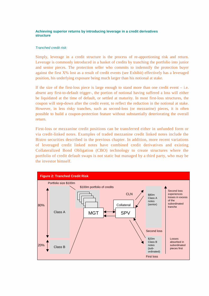
Achieving superior returns by introducing leverage in a credit derivativesstructure

Tranched credit risk:

Simply, leverage in a credit structure is the process of re-apportioning risk and return.Leverage is commonly introduced in a basket of credits by tranching the portfolio into juniorand senior pieces. The protection seller who commits to indemnify the protection buyeragainst the first X% lost as a result of credit events (see Exhibit) effectively has a leveragedposition, his underlying exposure being much larger than his notional at stake.

If the size of the first-loss piece is large enough to stand more than one credit event – i.e.absent any first-to-default trigger-, the portion of notional having suffered a loss will eitherbe liquidated at the time of default, or settled at maturity. In most first-loss structures, thecoupon will step-down after the credit event, to reflect the reduction in the notional at stake.However, in less risky tranches, such as second-loss (or mezzanine) pieces, it is oftenpossible to build a coupon-protection feature without substantially deteriorating the overallreturn.

First-loss or mezzanine credit positions can be transferred either in unfunded form orvia credit-linked notes. Examples of traded mezzanine credit linked notes include theBistro securities described in the previous chapter. In addition, more recent variationsof leveraged credit linked notes have combined credit derivatives and existingCollateralized Bond Obligation (CBO) technology to create structures where theportfolio of credit default swaps is not static but managed by a third party, who may bethe investor himself.

Figure 2: Tranched Credit Risk

Class A

Class B

Collateral

SPV

$80mClass Anotes(senior)

$20mClass Bnotes(sub-ordinated)

CLN

$100m portfolio of credits

MGT

Portfolio size $100m

80%

20%

First loss

Second loss

Second lossexperienceslosses in excessof thesubordinatedtranche

Lossesabsorbed insubordinatedpieces first

First-to-default credit positions

In a first-to-default basket, the risk buyer typically takes a credit position in each creditequal to the notional at stake. After the first credit event, the first-to-default note (swap)stops and the investor no longer bears the credit risk to the basket. First-to-default CreditLinked Note will either be unwound immediately after the Credit Event – this is usuallythe case when the notes are issued by an SPV - or remain outstanding – this is often thecase with issuers - in which case losses on default will be carried forward and settled atmaturity. Losses on default are calculated as the difference between par and the final priceof a reference obligation, as determined by a bid-side dealer poll for reference obligations,plus or minus, in some cases, the mark-to-market on any embedded currency/interest rateswaps transforming the cashflows of the collateral.

First-to-default structures are substantially pair-wise correlation plays, and provideinteresting yield-enhancing opportunities in the current tight spread environment. The yieldon such structures is primarily a function of (i) the number of names in the basket, i.e. theamount of leverage in the structure and (ii) how correlated the names are. The first-to-defaultspread shall find itself between the worse credit’s spread and the sum of the spreads, closer tothe latter if correlation is low, and closer to the former if correlation is high (see Exhibit).Intuition suggests taking first-to-default positions to uncorrelated names with similar spreads(hence similar default probabilities), in order to maximize the steepness of the curve below,thus achieving a larger pick-up above the widest spread.

Returns can be further improved via the addition of a mark-to market feature, wherebythe investor also takes the mark-to-market on the outstanding credit default swaps.Valuation of that mark-to-market can be computed by comparing the reference spread toan offer-side dealer poll of credit default swap spreads.

Investor

Par

Par minus net losses

Libor + x bps

Figure 3: First-to-default spread curve

0

0% 10%

20%

30%

40%

50%

60%

70%

80%

90%

100%

Correlation

20

40

60

80

100

120

≈ widest individual spread

≈ sum of all spreads

An alternative way to create a leveraged position for the investor is to use zero couponstructures, i.e. delay the coupon payments in a credit linked note, and reinvest the accruals.

De-leveraging exposures to riskier credit through a degree of capital and/orcoupon protection

Finally, leverage can be introduced by overlaying a degree of optionality for the protectionbuyer’s benefit. Substitution options whereby the protection buyer has the right tosubstitute some of the names in the basket, by another pre-defined set of names or anyother credit but subject to a number of guidelines, allow for significant yield enhancement.

By providing the flexibility to customize the riskyness of cashflows, credit derivativestructures can alternatively be used as a way to access new, riskier asset classes. An investorwith a high-grade corporates portfolio of credits may want to invest in a high-yield name,without significantly altering the overall risk profile of his holdings. This can be done byprotecting part or whole of the principal of a swap/note. In some case, a minimum guaranteedcoupon might be offered in addition to principal protection.

Example 1:

A 20-year USD capital-guaranteed credit linked note on Venezuela can be decomposedinto a combination of (i) a zero-coupon Treasury and (ii) a series of Venezuela-linkedannuity-like streams representing the coupons purchased from the note proceeds lessthe cost of the Treasury strip

While, as mentioned earlier, delaying the interest payments can be a powerful mean toenhance returns, equally, the leverage thus created can be significant.

Example 2:

Consider a 15-year zero-coupon structure on an emerging market/high yield credit where acredit event occurs after 13 years: the accrued amount lost this close to maturity issignificant. Some investors may not want or may not be allowed (for regulatory purposes)to put such a large amount of coupon at stake. Such risk can be reduced by building-in anaccruals lock-in feature, whereby if a credit event occurs, the investor receives, at maturity,whatever coupon amount has accrued up to the credit event date.

To summarize, we have seen that credit derivatives allow investors to invest in a widerange of assets with tailored risk-return profile to suit their specific requirements. Theasset can be a credit play on a portfolio of names, with or without leverage. We have alsoseen how to add a degree of credit exposure into a non-credit product, via an overlaymechanism. The nature and extent of the credit risk embedded in an asset determines thepricing of the asset, which is the focus of the next chapter.

Predictive or theoretical pricing models of Credit Swaps

A common question when considering the use of Credit Swaps as an investment or a riskmanagement tool is how they should correctly be priced. Credit risk has for many yearsbeen thought of as a form of deep out-of-the-money put option on the assets of a firm. Tothe extent that this approach to pricing could be applied to a Credit Swap, it could also beapplied to pricing of any traditional credit instrument. In fact, option pricing models havealready been applied to credit derivatives for the purpose of proprietary “predictive” or“forecasting” modeling of the term structure of credit spreads.

A model that prices default risk as an option will require, directly or implicitly, as parameterinputs both default probability and severity of loss given default, net of recovery rates, ineach period in order to compute both an expected value and a standard deviation or“volatility” of value. These are the analogues of the forward price and implied volatility in astandard Black-Scholes model.

However, in a practical environment, irrespective of the computational or theoreticalcharacteristics of a pricing model, that model must be parameterized using either market dataor proprietary assumptions. A predictive model using a sophisticated option-like approachmight postulate that loss given default is 50% and default probability is 1% and derive thatthe Credit Swap price should be, say, 20 b.p. A less sophisticated model might value a creditderivative based on comparison with pricing observed in other credit markets (e.g., if theundrawn loan pays 20 b.p. and bonds trade at LIBOR + 15 b.p., then, adjusting for liquidityand balance sheet impact, the Credit Swap should trade at around 25 b.p.). Yet the moresophisticated model will be no more powerful than the simpler model if it uses as its sourcedata the same market information. Ultimately, the only rigorous independent check of theassumptions made in the sophisticated predictive model can be market data. Yet, in asense, market credit spread data presents a classic example of a joint observation problem.Credit spreads imply loss severity given default, but this can only be derived if one isprepared to make an assumption as to what they are simultaneously implying about defaultlikelihoods (or vice versa). Thus, rather than encouraging more sophisticated theoreticalanalysis of credit risk, the most important contribution that credit derivatives will make to thepricing of credit will be in improving liquidity and transferability of credit risk and hence inmaking market pricing more transparent, more readily available, and more reliable.

4. Pricing Considerations

Mark-to-market and valuation methodologies for Credit Swaps

Another question that often arises is whether Credit Swaps require the development ofsophisticated risk modeling techniques in order to be marked-to-market. It is important inthis context to stress the distinction between a user’s ability to mark a position to market(its “valuation” methodology) and its ability to formulate a proprietary view on the correcttheoretical value of a position, based on a sophisticated risk model (its “predictive” or“forecasting” methodology). Interestingly, this distinction is recognized in the existingbank regulatory capital framework: while eligibility for trading book treatment of, forexample, interest rate swaps depends on a bank’s ability to demonstrate a crediblevaluation methodology, it does not require any predictive modeling expertise.

Fortunately, given that today a number of institutions make markets in Credit Swaps,valuation may be directly derived from dealer bids, offers or mid market prices (asappropriate depending on the direction of the position and the purpose of the valuation).Absent the availability of dealer prices, valuation of Credit Swaps by proxy to other creditinstruments is relatively straightforward, and related to an assessment of the market creditspreads prevailing for obligations of the Reference Entity that are pari passu with theReference Obligation, or similar credits, with tenor matching that of the Credit Swap, ratherthan that of the Reference Obligation itself. For example, a five-year Credit Swap on XYZCorp. in a predictive modeling framework might be evaluated on the basis of a postulateddefault probability and recovery rate, but should be marked-to-market based upon prevailingmarket credit spreads (which as discussed above provide a joint observation of impliedmarket default probabilities and recovery rates) for five-year XYZ Corp. obligationssubstantially similar to the Reference Obligation (whose maturity could exceed five years).If there are no such five-year obligations, a market spread can be interpolated or extrapolatedfrom longer and/or shorter term assets. If there is no prevailing market price for pari passuobligations to the Reference Obligation, adjustments for relative seniority can be made tomarket prices of assets with different priority in a liquidation. Even if there are no currentlytraded assets issued by the Reference Entity, then comparable instruments issued by similarcredit types may be used, with appropriately conservative adjustments. Hence, it should bepossible, based on available market data, to derive or bootstrap a credit curve for anyreference entity.

Constructing a Credit Curve from Bond Prices

In order to price any financial instrument, it is important to model the underlying risks onthe instrument in a realistic manner. In any credit linked product the primary risk lies inthe potential default of the reference entity: absent any default in the reference entity, theexpected cashflows will be received in full, whereas if a default event occurs the investorwill receive some recovery amount. It is therefore natural to model a risky cashflow as aportfolio of contingent cashflows corresponding to these different default scenariosweighted by the probability of these scenarios.

Example: Risky zero coupon bond with one year to maturity.

At the end of the year there are two possible scenarios:

1. The bond redeems at par; or2. The bond defaults, paying some recovery value, RV.

The decomposition of the zero coupon bond into a portfolio of contingent cashflows istherefore clear1.

PV

(1 - P D)

P D)RV

100

PV = [(1 - PD ) X 100 + PD X RV]

Recovery Value

(1 + r risk free)

1

This approach was first presented by R. Jarrow and S. Turnbull (1992): “Pricing Optionson Financial Securities Subject to Default Risk”, Working Paper, Graduate School ofManagement, Cornell University.

This approach to pricing risky cashflows can be extended to give a consistent valuationframework for the pricing of many different risky products. The idea is the same as thatapplied in fixed income markets, i.e. to value the product by decomposing it into itscomponent cashflows, price these individual cashflows using the method described aboveand then sum up the values to get a price for the product.

This framework will be used to value more than just risky instruments. It enables thepricing of any combination of risky and risk free cashflows, such as capital guaranteednotes - we shall return to the capital guaranteed note later in this section, as an example ofpricing a more complex product. This pricing framework can also be used to highlightrelative value opportunities in the market. For a given set of probabilities, it is possible tosee which products are trading above or below their theoretical value and hence use thisframework for relative value position taking.

Calibrating the Probability of Default

The pricing approach described above hinges on us being able to provide a value for theprobability of default on the reference credit. In theory, we could simply enterprobabilities based on our appreciation of the reference name’s creditworthiness andprice the product using these numbers. This would value the product based on our viewof the credit and would give a good basis for proprietary positioning. However, thisapproach would give no guarantee that the price thus obtained could not be arbitragedagainst other traded instruments holding the same credit risk and it would make itimpossible to risk manage the position using other credit instruments.

In practice, the probability of default is backed out from the market prices of tradedmarket instruments. The idea is simple: given a probability of default and recovery value,it is possible to price a risky cashflow. Therefore, the (risk neutral) probability of defaultfor the reference credit can be derived from the price and recovery value of this riskycashflow. For example, suppose that a one year risky zero coupon bond trades at 92.46and the risk free rate is 5%. This represents a multiplicative spread of 3% over the riskfree rate, since:

100

(1 + 0.05)(1 + 0.03)= 92.46

If the bond had a recovery value of zero, from our pricing equation we have that:

1

(1.05)92.46 = [(1 - PD) x 100 + PD x 0]

and so:

PD = 1 —(1.03)

1

So the implied probability of default on the bond is 2.91%. Notice that under the zerorecovery assumption there is a direct link between the spread on the bond and the probabilityof default. Indeed, the two numbers are the same to the first order. If we have a non-zerorecovery the equations are not as straightforward, but there is still a strong link between thespread and the default probability:

100(1 + s)

11 —

=PD

(100 — RV)≈

(1 — RV / 100)

s

This simple formula provides a “back-of-the-envelope” value for the probability of defaulton an asset given its spread over the risk free rate. Such approximation must, of course, beused with the appropriate caution, as there may be term structure effects or convexityeffects causing inaccuracies, however it is still useful for rough calculations.

This link between credit spread and probability of default is a fundamental one, and isanalogous to the link between interest rates and discount factors in fixed income markets.Indeed, most credit market participants think in terms of spreads rather than in terms ofdefault probabilities, and analyze the shape and movements of the spread curve rather thanthe change in default probabilities. However, it is important to remember that the spreadsquoted in the market need to be adjusted for the effects of recovery before defaultprobabilities can be computed. Extra care must be taken when dealing with EmergingMarket debt where bonds often have guaranteed principals or rolling guaranteed coupons.The effect of these features needs to be stripped out before the spread is computed asotherwise, an artificially low spread will be derived.

Problems Encountered in Practice

In practice it is rare to find risky zero coupon bonds from which to extract defaultprobabilities and so one has to work with coupon bonds. Also the bonds linked to aparticular name will typically not have evenly spaced maturities. As a result, it becomesnecessary to make interpolation assumptions for the spread curve, in the same manner aszero rates are bootstrapped from bond prices. Naturally, the spread curve and hence thedefault probabilities will be sensitive to the interpolation method selected and this willaffect the pricing of any subsequent products.

Assumptions need to be made with respect to the recovery value as it is impossible, inpractice, to have an accurate recovery value for the assets. It is clear from the equationsabove that the default probability will depend substantially on the assumed recoveryvalue, and so this parameter will also affect any future prices taken from our spreadcurve.

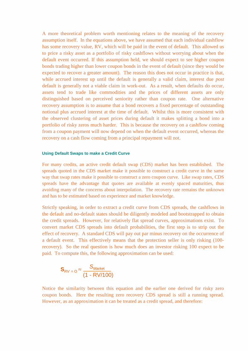
A more theoretical problem worth mentioning relates to the meaning of the recoveryassumption itself. In the equations above, we have assumed that each individual cashflowhas some recovery value, RV, which will be paid in the event of default. This allowed usto price a risky asset as a portfolio of risky cashflows without worrying about when thedefault event occurred. If this assumption held, we should expect to see higher couponbonds trading higher than lower coupon bonds in the event of default (since they would beexpected to recover a greater amount). The reason this does not occur in practice is that,while accrued interest up until the default is generally a valid claim, interest due postdefault is generally not a viable claim in work-out. As a result, when defaults do occur,assets tend to trade like commodities and the prices of different assets are onlydistinguished based on perceived seniority rather than coupon rate. One alternativerecovery assumption is to assume that a bond recovers a fixed percentage of outstandingnotional plus accrued interest at the time of default. Whilst this is more consistent withthe observed clustering of asset prices during default it makes splitting a bond into aportfolio of risky zeros much harder. This is because the recovery on a cashflow comingfrom a coupon payment will now depend on when the default event occurred, whereas therecovery on a cash flow coming from a principal repayment will not.

Using Default Swaps to make a Credit Curve

For many credits, an active credit default swap (CDS) market has been established. Thespreads quoted in the CDS market make it possible to construct a credit curve in the sameway that swap rates make it possible to construct a zero coupon curve. Like swap rates, CDSspreads have the advantage that quotes are available at evenly spaced maturities, thusavoiding many of the concerns about interpolation. The recovery rate remains the unknownand has to be estimated based on experience and market knowledge.

Strictly speaking, in order to extract a credit curve from CDS spreads, the cashflows inthe default and no-default states should be diligently modeled and bootstrapped to obtainthe credit spreads. However, for relatively flat spread curves, approximations exist. Toconvert market CDS spreads into default probabilities, the first step is to strip out theeffect of recovery. A standard CDS will pay out par minus recovery on the occurrence ofa default event. This effectively means that the protection seller is only risking (100-recovery). So the real question is how much does an investor risking 100 expect to bepaid. To compute this, the following approximation can be used:

(1 - RV/100)≈ SMarketSRV = O

Notice the similarity between this equation and the earlier one derived for risky zerocoupon bonds. Here the resulting zero recovery CDS spread is still a running spread.However, as an approximation it can be treated as a credit spread, and therefore:

Default probability ≈1(1 + SRV=0)

—1

t

This approximation is analogous to using a swap rate as a proxy for a zero coupon rate.Although it is really only suitable for flat curves, it is still useful for providing a quickindication of what the default probability is. Combining the two equations above:

Default probability ≈1

1 RV/100

SMarket1 +

1t

Linking the Credit Default Swap and Cash markets

An interesting area for discussion is that of the link between the bond market and the CDSmarket. To the extent that both markets are trading the same credit risk we should expectthe prices of assets in the two markets to be related. This idea is re-enforced by theobservation that selling protection via a CDS exactly replicates the cash position of beinglong a risky floater paying libor plus spread and being short a riskless floater paying liborflat1 . Because of this it would be natural to expect a CDS to trade at the same level as anasset swap of similar maturity on the same credit.

However, in practice we observe a basis between the CDS market and the asset swapmarket, with the CDS market typically – but not always - trading at a higher spread than theequivalent asset swap. The normal explanations given for this basis are liquidity premiaand market segmentation. Currently the bond market holds more liquidity than the CDSmarket and investors are prepared to pay a premium for this liquidity and accept a lowerspread. Market segmentation often occurs because of regulatory constraints which preventcertain institutions from participating in the default swap market even though they areallowed to source similar risk via bonds. However, there are also participants who aremore inclined to use the CDS market. For example, banks with high funding costs caneffectively achieve Libor funding by sourcing risk through a CDS when they may payabove Libor to use their own balance sheet.

Another more technical reason for a difference in the spreads on bonds and default swapslies in the definition of the CDS contract. In a default swap contract there is a list ofobligations which may trigger a credit event and a list of deliverable obligations whichcan be delivered against the swap in the case of such an event. In Latin Americanmarkets the obligations are typically all public external debt, whereas outside of LatinAmerica the obligations are normally all borrowed money. If the obligations are allborrowed money this means that if the reference entity defaults on any outstanding bondor loan a default event is triggered. In this case the CDS spread will be based on thespread of the widest obligation. Since less liquid deliverable instruments will often tradeat a different level to the bond market this can result in a CDS spread that differs from thespreads in the bond market.

For contracts where the obligations are public external debt there is an arbitrage relationwhich ties the two markets and ought to keep the basis within certain limits.Unfortunately it is not a cheap arbitrage to perform which explains why the basis cansometimes be substantial. Arbitraging a high CDS spread involves selling protection viathe CDS and then selling short the bond in the cash market. Locking in the difference inspreads involves running this short position until the maturity of the bond. If this is donethrough the repo market the cost of funding this position is uncertain and so the positionhas risk, including the risk of a short squeeze if the cash paper is in short supply.However, obtaining funding for term at a good rate is not always easy. Even if thefunding is achieved, the counterparty on the CDS still has a credit exposure to thearbitrageur. It will clearly cost money to hedge out this risk and so the basis has to be bigenough to cover this additional cost. Once both of these things are done the arbitrage iscomplete and the basis has been locked in. However, even then, on a mark-to-marketbasis the position could still lose money over the short term if the basis widens further. Soideally, it is better to account for this position on an accrual basis if possible.

Using the Credit Curve

As an example of pricing a more complex structure off the credit curve, we shall nowwork through the pricing of a 5 year fixed coupon capital guaranteed credit-linked note.This is a structure where the notional on the note is guaranteed to be repaid at maturity(i.e. is not subject to credit risk) but all coupon payments will terminate in the event of adefault of the reference credit. The note is typically issued at par and the unknown is thecoupon paid to the investor. For our example we shall assume that the credit defaultspreads and risk free rates are as given in Table 1:

Table 1: Cumulative Default Probabilities

Year Risk Free CDS Spread Cumulative default prob1

1 5.00% 7.00% 7.22%

2 5.00% 7.00% 13.91%

3 5.00% 7.00% 20.13%

4 5.00% 7.00% 25.89%

5 5.00% 7.00% 31.24%

The capital guaranteed note can be decomposed into a risk-free zero coupon bond and azero recovery risky annuity, with the zero coupon bond representing the notional on thenote and the annuity representing the coupon stream. As the zero coupon bond carries nocredit risk it is priced off the risk free curve. In our case:

100

Zero Price =(1.05)5

= 78.35

So all that remains is to price the risky annuity. As the note is to be issued at par, theannuity component must be worth 100 - 78.35 = 21.65. But what coupon rate does thiscorrespond to? Suppose the fixed payment on the annuity is some amount, C. Eachcoupon payment can be thought of as a risky zero coupon bond with zero recovery. So wecan value each payment as a probability-weighted average of its value in the default and nodefault states as illustrated in Table 2:

Table 2: Coupon paid under a capital-protected structure

Y e a r Disco u n t Factor F o rw a r d V a l u e P V

1 0.9524 C*0.9278 + 0*0 .0722 C*0.8837

2 0.9070 C*0.8609 + 0*0 .1391 C*0.7808

3 0.8638 C* 0.7988 + 0*0 .2013 C*0.6900

4 0.8227 C*0.7411 + 0*0 .2589 C*0.6097

5 0.7835 C*0.6876 + 0*0 .3124 C*0.5388

So the payment on the annuity should be:

C = 21.65 / (0.8837 + 0.7808 + 0.6900 + 0.6097 + 0.5388)C = 6.18

81.68(78.35 + 3.33)

Valuing a fixed coupon capital guaranteed note

6.186.18 6.18 6.18

1 2 3 45.46

4.83

4.263.77

Risky

Risk Free

6.18

100

5

Counterparty considerations: pricing the two-name exposure in a creditdefault swap

In a credit swap the Protection Buyer has credit exposure to the Protection Sellercontingent on the performance of the Reference Entity. If the Protection Seller defaults,the Buyer must find alternative protection and will be exposed to changes inreplacement cost due to changes in credit spreads since the inception of the originalswap. More seriously, if the Protection Seller defaults and the Reference Entitydefaults, the Buyer is unlikely to recover the full default payment due, although the finalrecovery rate on the position will benefit from any positive recovery rate on obligationsof both the Reference Entity and the Protection Seller.

Counterparty risk consequently affects the pricing of credit derivative transactions.Protection bought from higher-rated-counterparties will command a higher premium.Furthermore, a higher credit quality premium; protection purchased from a counterpartyagainst a Reference Entity is less valuable if a simultaneous default on the two nameshas a higher probability.

The problem of how to compute and charge for counterparty credit exposure is in largepart an empirical one, since it depends on computing the joint likelihood of arriving indifferent credit states, which will in turn depend on an estimate of credit qualitycorrelation between the Protection Seller and Reference Entity, which cannot be directlyobserved. Fortunately, significant efforts have been undertaken in the area of defaultcorrelation estimation in connection with the development of credit portfolio models suchas CreditMetrics.

The following expression describes a simple methodology for computing a “counterpartycredit charge” (CCC), as the sum of expected losses due to counterparty (CP) defaultacross N different time periods, t, and states of credit quality (R) of the Reference Entity(RE) from default through to AAA. Given an estimate of credit quality correlation, it ispossible to estimate the joint likelihood of the Reference Entity being in each state,given a counterparty default, from the respective individual likelihoods or arriving ineach state of credit quality. Since loss can only occur given a default of thecounterparty, we are interested only in the default likelihood of the counterparty.However, since loss can occur due to changes in the mark-to-market (MTM) of theCredit Swap caused by credit spread fluctuations across different states of theReference Entity, we are interested in the full matrix of credit quality migrationlikelihoods of the Reference Entity.

Typically, the counterparty credit charge is subtracted from the premium paid to theProtection Seller and accounted for by the Protection Buyer as a reserve againstcounterparty credit losses.

CCC = (100% - Recovery Rate CP )* Σ Σ Prob Joint {CP In defaultRERating = R } * Op Rating = R

CP = Counterparty

RE = Reference Entity

N = Number of time periods, t

R = Rating of the Reference Entity in time t

Op = Price of an option to replace a risky exposure to RE instate R at time t with ariskless exposure, ie. When RE has defaulted, value is (100% - Recovery Rate RE)ie. When RE has not defauled , value is (100% - MTM of Credit Swap, based on creditspreads)

tN AAA

t=t0 R=Def

The evolution of the credit derivatives has not been an isolated event. The facility affordedby credit derivatives to more actively manage credit risk is certainly notable in its own right.However, this facility to manage risk would be incomplete without methods to identifycontributors to portfolio risk. Not surprisingly, the advent of public portfolio credit riskmodels has coincided with the growth of the credit derivatives markets. The models nowallow market participants to recognize sources of risk, while credit derivatives provideflexibility to manage these sources.

In this chapter, we will survey the various publicly available credit models, and describethe CreditMetrics model in greater detail. We will then describe a number of practical usesof the CreditMetrics model.

Credit portfolio models – a survey

The year 1997 was an important one for the analysis of credit portfolios, with thepublication of three models for portfolio credit risk. In order of publication, the modelswere:

•

CreditMetrics, published as a technical document by J.P.Morgan, and now furtherdeveloped by the RiskMetrics Group,k LLC, who also markets a softwareimplementation, CreditManager,

CreditRisk + published as a technical document by CreditSuisse, FinanacialProducts, and

Credit Portfolio View, published as two articles in Risk magazine by ThomasWilson of McKinsey and Company.

Thus, in the span of just over six months, the number of publicly documented modelsfor assessing portfolio risk grew from zero to three. That there were three differingapproaches to the same problem might have led to an emphasis on modelingdiscrepancies, but it led instead to a greater emphasis that the problem – credit risk ina portfolio context – was crucial to address.

5. CreditMetrics – A portfolio approach to credit riskmanagemen

The three models above, and indeed any conceivable model of portfolio credit risk,share two features. The first is the treatment of default as a significant downwardjump in exposure value, which necessitates default probabilities and loss severitiesas inputs; the second is the development of some structure to describe thedependency between defaults of individual names.

It is important to realize that none of the three models above provide the defaultprobabilities of individual names as output, and so all three must rely on external sourcesfor this parameter. In fact, the default probability for a given issuer or counterparty isanalogous to the volatility of an asset when considering market risk; that is, it is theforemost (though not necessarily only) descriptor of the stand alone risk of the exposure inquestion. However, the situation in credit risk is more complicated. For an exposure to aforeign currency, it is possible to observe that currency’s exchange rate over time andarrive at a reasonable estimate of the rate’s volatility. For an exposure to a particularcounterparty, looking at the counterparty’s history tells us nothing about its likelihood ofdefaulting in the future; in fact, that we have an exposure at all is a likely indication thatthe counterparty has not defaulted before, though it certainly could default in the future.

Since the examination of individual default histories is not helpful, a number ofmethods have been developed to estimate default probabilities. The first is to score orrank individual names, categorize names historically according to their credit score,and then measure the proportion of similar names that have defaulted over time. Thisis the approach taken by the rating agencies, wherein they have credit ratings (scores)for a vast array of names and over a long history, and report, for example, theproportion of A-rated names that default within one year. For portfolio models, it ispossible to extrapolate from this information, and assign A-rated names the historicaldefault probability for that rating. For names large enough to carry ratings, the resultsprovided by the agencies are most commonly used because of the widespreadacceptance of their ratings and the large coverage and history of their databases. Forsmaller, non-rated names, other credit scoring systems can be utilized in a similarvein. Additionally, this approach can be extended to one where the fluctuation ofdefault rates over time is explained by factors such as interest rates, inflation, andgrowth in productivity.

Clearly, the approach mentioned above involves a tradeoff: historical default informationbecomes useful, but at the expense of granularity. That is, it is necessary to sacrifice namespecific information, and use default probabilities that are only particular to a given creditrating or score. In order to ascertain the default probability for a particular name, the twomost common methods utilize, where possible, current market information rather thanhistory. One approach is to observe the price of a name’s traded debt, and to suppose thatthe discrepancy between this price and the price of a comparable government security isattributable to the possibility that the name may default on its debt. A second approach isto utilize the equity markets, and extract a firm’s default probability from its equity price,the structure of its liabilities, and the observation that equity is essentially a call option onthe assets of the firm.2

While the three models each treat the value changes resulting from defaults, and thusrequire default probabilities as inputs, the CreditMetrics model also treats value changesarising from significant changes in credit quality, such as a ratings downgrade, short ofdefault. This additional capacity of the model necessitates additional data, namely theprobabilities of such quality changes. The probabilities are available also from theagency approaches mentioned above. We will discuss this data further in the nextsection.

The most significant structural difference between the three models is in how theyconstruct dependencies between defaults. The CreditRisk+ model builds dependencies bystipulating that all names are subject to one or more systemic and volatile default rates. Inthe simplest case, all names depend on one default rate. In some scenarios, the rate is highand all the names have a greater chance of defaulting, while in others the rate is lower, andthe names all have a lesser chance of defaulting. The default probabilities discussed earlierrepresent the average default rate in this context. The dependence of many names on amutual default rate essentially creates a correlation between the names, and the volatility ofthe default rate, which is an input to the model, determines the level of correlation. TheCredit Portfolio View model also treats the variation in default rates (and more generally,in rating change probabilities) but rather than simply assigning a volatility to the rate, themodel explains the fluctuations in the default rate through fluctuations in macroeconomicvariables. In the CreditMetrics model, rather than explaining a systemic factor like thedefault rate, we model each name’s default as contingent on fluctuations in the assets of theindividual firm. The dependency between individual defaults is then built by modeling thecorrelations between firm asset values.

Although there appear to be fundamental differences in the three approaches; in factthe frameworks are quite similar. Naturally, the publication of so many approacheswas followed by efforts to compare them. The consensus of the comparisons has beenthat if the model inputs are set consistently, the models will give very similar results.Empirical comparisons have shown some discrepancies, though due to inconsistentmodel inputs rather than disparities in the model frameworks. Thus, the burden haspassed from developing frameworks to identifying good data.

We move now to a more detailed discussion of the CreditMetrics model and itsrequired imputs.

An overview of the CreditMetrics model

As we have already discussed, CreditMetrics models the changes in portfolio valuethat result from significant credit quality moves, that is, defaults or rating changes.The model takes information on the individual obligors in the portfolio as inputs, andproduces as output the distribution of portfolio values at some fixed horizon in thefuture. From this distribution, it is possible to produce statistics which quantify theportfolio’s absolute risk level, such as the standard deviation of value changes, or theworst case loss at a given level of confidence. While this gives a picture of the totalrisk of the portfolio, we may also analyze our risks at a finer level, examining the riskcontribution of each exposure in the portfolio, identifying concentration risks ordiversification opportunities, or evaluating the impact of a potential new exposure.Examples and applications of these outputs will be provided in the next section.Here, we describe the model itself in more detail.

The model is best described in three parts:

1. The definition of the possible “states” for each obligor’s creditquality , and a description of how likely obligors are to be in anyof these states at the horizon date.

2. The interaction and correlation between credit migrations ofdifferent obligors.

3. The revaluation of exposures in all possible credit states.

Step 1 – the states of the world

The definition of an obligor’s possible credit states typically amounts to selecting arating system, whether an agency system or an internal one, whether a coarse systemwith seven states, or a fine one with plus or minus states added. The crucial elementhere is that we know the probabilities that the obligor migrates to any of the statesbetween now and the horizon date. That the user provides this information to themodel is what differentiates CreditMetrics from a credit scoring model. The moststraightforward way to present the probabilities is through a transition matrix; anexample appears in Table 1. A transition matrix characterizes a rating system byproviding the probabilities of migration (within a specified horizon) for all of thesystem’s states.

Table 1: Example one-year transition matrix - Moody’s rating system

Aaa Aa A Baa Ba B Caa DAaa 93.38% 5.94% 0.64% 0.00% 0.02% 0.00% 0.00% 0.02%Aa 1.61% 90.53% 7.46% 0.26% 0.09% 0.01% 0.00% 0.04%A 0.07% 2.28% 92.35% 4.63% 0.45% 0.12% 0.01% 0.09%Baa 0.05% 0.26% 5.51% 88.48% 4.76% 0.71% 0.08% 0.15%Ba 0.02% 0.05% 0.42% 5.16% 86.91% 5.91% 0.24% 1.29%B 0.00% 0.04% 0.13% 0.54% 6.35% 84.22% 1.91% 6.81%Caa 0.00% 0.00% 0.00% 0.62% 2.05% 4.08% 69.19% 24.06%

Among the most widely available transition matrices are those produced by the majorrating agencies, which reflect the average annual transition rates over a long history(typically 20 years or more) for a particular class of issuers (e.g. corporate bonds orcommercial paper). While this information is useful, and the agency default rates havebecome benchmarks for describing the individual categories, the use of average transitionmatrices for credit portfolio modeling is often criticized for its failure to capture the creditcycle. In other words, since the matrices only represent averages over many years, theycannot account for the current year’s credit transitions being relatively benign or severe.A number of methods are now available to address this. One is to select smaller periodsof the agency history, and create matrices based, for example, only on the transitions in1988 to 1991. A second is to explicitly model the relationship between transitions anddefaults and macroeconomic variables, such as spread levels or industrial production.Regardless of the transition matrix ultimately chosen as the “best”, because of thedifficulties inherent in default rate estimation, it is prudent to examine the portfolio undera variety of transition assumptions.

Step 2 – revaluation

While the first step concerns the description of migrations of individual credits, tocomplete the picture, we need a notion of the value impact of these moves. This bringsup the issue of revaluation. In short, we assume a particular instrument’s value today isknown, and wish to estimate its value, at our risk horizon, conditional on any of thepossible credit migrations that the instrument’s issuer might undergo.

Consider a Baa-rated, three year, fixed 6% coupon bond, currently valued at par. With aone year horizon, the revaluation step consists of estimating the bond’s value in one yearunder each possible transition. For the transition to default, we value the bond through anestimate of the likely recovery value. Many institutions use their own recoveryassumptions here, although public information is available. For the non-default states, weobtain an estimate of the bond’s horizon value by utilizing the term structure of bondspreads and risk-free interest rates. In the end, we arrive at the values in Table 2. With theinformation in Table 2, we have all of the stand-alone information for this bond;consequently, we can calculate the expectation and standard deviation of the bond’s valueat the horizon.

Rating at horizon

Probability Accrued Coupon

Bond value

Bond plus coupon

Aaa 0.05% 6.0 100.4 106.4Aa 0.26% 6.0 100.3 106.3

A 5.51% 6.0 100.1 106.1

Baa 88.48% 6.0 100.0 106.0Ba 4.76% 6.0 98.5 104.5B 0.71% 6.0 96.2 102.2Caa 0.08% 6.0 93.3 99.3D 0.15% 6.0 40.1 46.1

Mean 99.8 105.8St. dev. 2.36 2.36

Table 2: Values at Horizon for three year 6% Baa bond

To incorporate other types of exposures only involves defining the values in eachpossible future rating state of the underlying credit. Essentially, this amounts tobuilding something like Table 2. For some exposure types (for example, bonds andloans), all that is necessary to build this table are recovery assumptions and spreads,while for others (commitment lines or derivative contracts), further information isrequired. Assuming a riskless derivative counterparty, the simple credit derivatives ofthe previous chapter can be incorporated in the same way. To account forcounterparty risk as well involves some slight enhancements, but is not complicated.1

Step 3 – building correlations

The final step is to construct correlations between exposures. To do this, we posit anunseen "driver" of credit migrations, which we think of as changes in asset value. Ourapproach is conceptually similar to, and certainly inspired by, the equity based modelsmentioned previously. The intuition behind these models is that default occurs whenthe value of a firm’s assets drops below the market value of its liabilities. In our case,we do not seek to observe asset levels, nor to use asset information to predict defaults;the stand-alone information for each name (in particular the name's probability ofdefault) is provided as a model input through the specification of the transition matrix.Rather, assets are used only to build the interaction between obligors.

To begin our construction of correlations, we assume that asset value changes arenormally distributed. We then partition the asset change distribution for each nameaccording to the name's transition probabilities. For the Baa-rated obligor above (withdefault probability equal to 0.15%), the default partition (which conceptually can bethought of as the obligor’s liability level) is chosen as the point beyond which lies 0.15%probability; the CCC partition is then chosen to match the obligor's probability ofmigrating to CCC, and so on. The result is illustrated in Figure 1.

Figure 1: Partition of asset change distribution for a Baa obliger

>3.32.7 → 3.31.5 → 2.7-1.6 → 1.5-2.4→ -1.6-2.8→ -2.4-3.0→ -2.8<-3.0

AaaAaABaaBaBCaaDefault

100.4100.3100.1100.098.596.293.340.1

Obligerdefaults Obliger

remains Baa

Asset return

New rating

Value

A common misinterpretation of this step is that by using a normal distribution for assetvalue changes, we are somehow not accounting for the well documented non-normality inthe returns of credit driven assets. This is not the case, as it is only the driver of creditchanges for which we assume a normal distribution, but not the changes in asset valuesthemselves. In fact, if we consider the values (from Table 2) with the partition in Figure1, we see that a two standard deviation increase in asset value produces an appreciation of0.1, whereas an equally likely two standard deviation decrease produces a depreciation of1.5; similarly, a three standard deviation asset value increase yields an appreciation of 0.3,but an equivalent decrease yields a depreciation of 59.9. This is the type of skew that isexpected in credit distributions.

In the portfolio framework, once the partitions are defined for every obligor, it onlyremains to describe the correlation between asset value changes. Rather than attempting toobserve these changes directly, we take correlations in equity returns as a proxy for theasset value correlations. This is primarily a practical decision, and allows us to thenestimate correlations using reliable data. As in the prior two steps, however, it is crucial toexamine the sensitivity of the model to uncertainties in the data. While the correlationestimates are designed to be stable and applicable over long horizons such as one year,market events may rapidly change correlation structures; to evaluate the impact of thesechanges, it is recommended to analyze the portfolio under both normal and "stressed"correlation conditions.1

With the correlations defined, the model is completely specified. In principle, it ispossible to explicitly calculate the probabilities of all joint rating transitions (e.g.obligor 1 defaults, obligor 2 downgrades, obligor 3 stays the same rating, etc.). Inpractice, it is faster to obtain the portfolio distribution through a Monte Carloapproach. Thus, for a single scenario, we draw from a multivariate normaldistribution to produce asset value changes, read from the partitions to identify thechanges with new rating states and exposure values, and aggregate the individualexposures to arrive at a portfolio value for the scenario. Examples of this process forstrongly and weakly correlated two obligor portfolios are illustrated in Figures 2 and3. Repeating this process over a large number of scenarios, we accumulate a largenumber of equally likely portfolio values, and are able to estimate the Value at Risk,and other descriptive statistics, of the portfolio.

Figure 2: Two Baa bonds, strong correlation. Mean=199.6, St.Dev.=4.13.

Applications

Estimation of economic capital

The first application of the approach outlined above is to evaluate the absolute risk ofa portfolio. To do so, it has become common to report the portfolio’s Value at Risk(VaR) – the maximum amount the portfolio might lose over a given time horizon,with a given level of confidence. For trading portfolios, it is common to report theVaR for a one day horizon with a 95% confidence level, corresponding roughly to themaximum portfolio daily loss over one month, or a ten day horizon with a 99%confidence level, corresponding to the maximum two week loss over a five yearperiod. In these cases, VaR is used mostly as a communication tool; traders andmanagers have intuition for the worst loss over these timeframes, and so VaR isinformative. For credit portfolios, with a horizon such as one year, even VaR at a lowconfidence level like 90% gives a worst case one year loss over a ten year period.

Beyond its use as a communication tool, VaR for credit portfolios is more appropriateto assess economic capital. For a bank investing in a portfolio on a funded basis, a keyquestion is how much capital needs to be allocated to cover worst case portfolio losses.At an institutional level, the question is how much capital the institution needs to protectagainst major downturns and guarantee solvency. In both cases, it is easy to frame theproblem in terms of VaR. Figure 4 presents a portfolio distribution that might resultfrom an application of CreditMetrics. The left-most vertical bar represents the valuebelow which the portfolio will fall with 0.1% probability; the second bar from the leftrepresents the level below which the portfolio will fall with 1% probability. Thus, withcapital equal to the distance from the mean value to the left-most bar, there is a 99.9%chance that the capital will be sufficient to absorb the portfolio loss, and thus only a0.1% chance of insolvency.

Figure 4: Portfolio distribution and economic capital

42 44 46 48 50

Portfolio value ($US Millions)

Mean value

99% worst case loss

99.9% worst case loss

.

With the availability of portfolio models and the visibility of agency transition matrices,it has become common for institutions to choose a target rating, and take the defaultprobability for this rating as a VaR confidence level. Thus, if an institution wishes tomaintain a Baa rating, they would take the 0.15% default probability from Table 1, andcompute their required economic capital at a 99.85% confidence level. Moreover, theinstitution would assess new transactions by their contribution to the capital at thislevel. In the remainder of this section, we will discuss the risk contribution outputs ofthe model, and how these may be used for active risk management.

Identification of risk reducing transactions

With the liquidity concerns that accompany credit portfolios, the portfolio manager isoften limited to decisions to continue to hold an exposure or to sell it entirely. Whilethe impact of a sale on the portfolio’s expected return is straightforward and involvesonly an analysis of the exposure in question, the risk impact of a sale involves the entireportfolio. Clearly, other things being equal, the sale of an exposure that represents anoverconcentration of the portfolio (whether to a single obligor or to an industry sector)will reduce portfolio risk more than the sale of an exposure that represents lessconcentration. To quantify this point, we define an exposure’s marginal risk as theamount the portfolio risk will be reduced were we to sell the exposure.

In Figure 5, we present the marginal risks for a sample portfolio. Each pointrepresents an exposure, with the exposure’s size indicated on the horizontal axis, andthe exposure’s marginal risk as a percent of its size indicated on the vertical axis. Foreach exposure, the product of its horizontal and vertical positions gives its totalmarginal risk; thus, curves such as the one in the figure indicate exposures with thesame risk contribution. We have identified the exposure to Obligor X, a Baa-ratedobligor in the financial sector, as the largest risk contributor.

Figure 5: Marginal risks for sample 50 bond portfolio

0%

2%

4%

6%

8%

10%

12%

0 1 2 3 4 5 6

Exposure Amount (US$Million)

Mar

gina

l St.

Dev

. %

Obligor X

Points of constant marginal risk

There are two factors that may account for the Obligor X exposure’s large riskcontribution. One is that it is very risky, even on a stand-alone basis; this could be the casehere, as the Obligor X exposure is quite large relative to the portfolio, and could embody asignificant obligor concentration. The second is that the exposure is strongly correlatedwith other exposures in the portfolio, and is contributing to a large industry or sectorconcentration. In general, these two factors act in concert, but we may investigate therelative importance of the two by examining a strategy that eliminates the correlation riskbut leaves the stand-alone risk unchanged.

The strategy is to sell the exposure to Obligor X, and replace the exposure by one withidentical stand-alone characteristics (coupon, credit rating, maturity, etc.) but with nocorrelation to the rest of the portfolio. In this way, the stand-alone risk is unchanged,but we eliminate any risk that derives from the Obligor X exposure’s dependence onother exposures. In our case, this provides a significant risk reduction. In Figure 6, wepresent the new marginal statistics, and see that what had been our largest riskcontributor is now in line with the other exposures. Additionally, we see in Table 3,that our reallocation has the effect of materially reducing the absolute portfolio risk,with no impact at all on expected return. While such an opportunity may not always beavailable, this example illustrates the benefits of better diversification, and suggests thatportfolio managers might seek out opportunities, whether through direct sales andpurchases as here or through derivative transactions, to manage their portfolioconcentrations.

Figure 6: Marginal risks for sample 50 bond portfolio, after reallocation

0%

2%

4%

6%

8%

10%

12%

0 1 2 3 4 5 6

Exposure Amount (USD millions)

Mar

gina

l St.

Dev

% Points of constant marginal risk

"New" Obligor X

Table 3: Effect of reallocation on portfolio risk

Before reallocation

After reallocation Reduction

Expected return 5.3% 5.3% 0%Standard deviation 659, 800 585, 100 11%5th Percentile loss 897, 700 856, 200 4.6%1st percentile loss 2,623, 000 2,483, 000 5.3%

Decisions to extend and price credit

While the previous analysis focused on existing exposures, it is often desirable to bemore prospective. When an asset manager faces the decision to take on a newexposure, or a bank ponders extending the credit of an existing obligor, it is necessaryto examine the effect of this new position on the portfolio risk. This effect will affectboth the choice to take on exposure, and how this exposure is priced. Ideally, we wouldlike run the model to reassess the portfolio given any potential transaction. In practice,we are not likely to conceive of every possible transaction we are likely to face, norwould the risk contribution of so many hypothetical deals be informative.

To reduce the problem, it is convenient to group our exposures – by rating andindustry sector, for example – and communicate the risk contribution of additionalexposure to these groups. Here, the marginal analysis of the previous section isless appropriate; we are not interested in the effect of removing a sector altogether,but rather in the effect of adding to the sector incrementally. Thus, in this case, wereport the impact of a small percentage increase in our exposure to each sector andrating. The results for the sample bond portfolio are presented in Figure 7 .

Figure 7: Incremental Standard deviation by credit rating and industry sector

Incr

emen

tal S

tand

ard

Dev

iatio

n

UtilitiesTechnologySovereignFinancialEnergy

40.0

20.0

0.0

80.0

60.00.70

50.0

30.0

10.0

B (Moodys 8-state)

Ba (Moodys 8-state)

Baa (Moodys 8-state)

A (Moodys 8-state)

Aa (Moodys 8-state)

Aaa (Moodys 8-state)

Not surprisingly, we see that Baa-rated obligors in the financial sector (such as ObligorX) will contribute more risk as we increase our exposure to this sector. In addition, Ba-rated exposures in the financial and energy sectors also represent high incremental risk,suggesting that credit be extended less liberally to these sectors, or at least that theseconcentrations be reflected in the pricing of further exposures. The higher ratings appearattractive for all sectors, though the returns here may not be as enticing as for the lowerratings. Most striking, however, is the diversification opportunity into Ba-rated obligorsin the energy sector, where there is the potential to obtain comparable yields to Ba-ratedfinancials or energy companies, but with a fraction of the incremental risk.

Risk-based credit limits

A third application of the model is to set credit limits based on risk contributions.Traditionally, limits have been set based on exposure size (e.g. no single exposure greaterthan $20 million) or on rating (e.g. no exposure to sub-investment grade names). We couldrepresent these limits by vertical and horizontal lines, respectively, on plots such as Figure5. As we discussed previously, however, points along the curve in Figure 5 representequal risk contributions; thus it is more sensible to set limits like the curves, stipulating thatan exposure contribute more than a given amount to portfolio risk.

Ultimately, we would like to link the exposure limit for each obligor to the returnavailable in the market for such an exposure. Obligor and industry concentrationeffects are such that the risk contribution of an individual obligor increases with the sizeof the exposure to the obligor; further, the risk increase is greater at higher exposurelevels. This relationship is illustrated in the left plot of Figure 8. For each increment inexposure to the obligor, a higher return is required to compensate for the increased risk.At some point, this required return will be greater than the return available. The pointof intersection between the required and available returns, as shown on the right ofFigure 8, should serve as a target for the exposure to the obligor.

Figure 8: Exposure targets based on risk-return tradeoffRisk-based pricing as a mechanism for “soft” limit setting

Size of total exposure to obligor

AAA

AA

A

BBB

BB

BRisk

Size of total exposure to obligor

Return

Available market return

Risk-based minimumrequired return

“Soft limit”

Impact of exposure size on risk

Conclusions

Employees of the RiskMetrics Group are often asked whether CreditMetrics (or for thatmatter, credit portfolio models in general) has succeeded. Perhaps the best way toevaluate its success is to return to three reasons given in 1997 for the release of themodel:

� To build liquidity and transparency in the credit markets,

� To improve the dialogue with regulators, and

� To improve the dialogue with clients

To the first point, while it would be presumptive to claim credit models as a cause, it islikely more than coincidental that volume and variety in the credit markets haveincreased steadily since 1997. New bond issuance in the United States hit a recordlevel in 1997, and increased a further 17% in 1998; meanwhile, the growth of issuersin the European Community has outpaced the rest of the world. In securitizations,particularly Collateralized Debt Obligations, where the understanding of portfolioeffects is crucial, yearly volume increased four-fold from 1996 to 1998, and is on pacefor another 20% gain in 1999. All of this has been accompanied by the rise of thecredit derivatives that are the subject of this volume.

Certainly, regulators took notice of the portfolio models, particularly given the modelsponsors’ implicit (and at times explicit) criticism of the Bank for InternationalSettlements (B.I.S.) capital rules. The Federal Reserve Bank of New York hosted aconference on the future of capital regulation in February, 1998, and the Bank of Englandand the Financial Services Authority hosted another conference on credit risk modelingin September, 1998. Following this interest were consultative papers by Committee onBanking Supervision of the B.I.S.: one in April, 1999 on the state of credit riskmodeling, and a second in June, 1999 proposing changes in the capital adequacyregulations. Though the proposed changes do not yet account for portfolio effects, theydo represent a significant step toward accurately recognizing credit quality in thecalculation of regulatory capital.

Lastly, the interest from clients has been overwhelming. JP Morgan and theRiskMetrics Group have distributed over 15,000 copies of the CreditMetricsTechnical Document, while the CreditMetrics website continues to receive three tofive thousand hits per month. CreditManager, the software implementation of themodel, is now installed at over 100 institutions worldwide. As volume and liquiditycontinue to increase, particularly in Europe and emerging markets, and asopportunities for risk management through derivatives continue to develop, weexpect the interest in credit portfolio models to only accelerate in the future.

References:

CreditRisk+: A credit risk managementframework, London: Credit Suisse FinancialProducts, 1997.

Finger, C.C.: A methodology to stresscorrelations, RiskMetrics Monitor, Fourthquarter, 1997.

Finger, C.C.: Sticks and Stones, Workingpaper, RiskMetrics Group, LLC, 1998

Finger, C.C.: Credit Derivatives inCreditMetrics, CreditMetrics Monitor, Thirdquarter, 1998

Gluck, J.: 1999 First Quarter CDO Review,Moody’s Special Report, April, 1999

Gordy, M.: A Comparative Anatomy of CreditRisk Models, Federal Reserve Board FEDS1998-47, December 1998

Gupton, G.M., Finger, C.C., and Bhatia, M.:CreditMetrics - Technical document, NewYork: Morgan Guaranty Trust Co., 1997

Jarrow, R.A., and Turnbull, S.M.: Pricingderivatives

on financial securities subject to credit risk,The Journal of Finance, Vol. L, No.1, March1995

Keenan, S.C. Shotgrin, I. And Sobehart,J.: Historical default rates of corporate bondissuers, 1920-1998, Moody’s InvestorsService, January 1999.

Kim, J.: A way to condition transition matrixon wind, Working paper, RiskMetrics Group,LLC, 1999

Kolyoglu, Ugur and Hickman, A.:Reconcilable Differences, Risk, October1998

Merton, R.: On the Pricing of CorporateDebt: The Risk Structure of Interest Rates,The Journal of Finance, 1994.

Standard & Poor’s: Ratings Performance1998 - Stability & Transition. March 1999.

Wilson, T.: Portfolio Credit Risk I, Riskmagazine, September, 1997.

Wilson, T.: Portfolio Credit Risk II, Riskmagazine, October 1997.

The advent of credit derivatives to the international banking forum has yet to begreeted with a definitive regulatory response from the Bank of InternationalSettlements (BIS) for uniform global application. Rather, regulators regionally,through their publication of guidelines for banks within their respective jurisdictions,have part fuelled and part responded to the rapid growth of the credit derivativesmarket, a growth which has seen, in the U.S. alone, volume in terms of notionaloutstanding increase by over 400% over the last two years.1

This chapter outlines the regulatory approach to credit derivatives and discussescertain variations in the treatments of specific issues from jurisdiction to jurisdiction.

Treatment of credit derivatives in the Banking Book

The reduction in risk effected though buying protection on an asset via a creditderivative is seen as analogous to that afforded by a bank guarantee on that asset, and inconsequence the regulatory approach to the former is consistent with the well-established approach to the latter as set forth in the Basle Capital Accord.1

‘Unfunded’ credit derivatives

As the credit exposure of the Protection Seller to the Reference Entity in a creditderivative transaction is substantially identical to that of a lender to or bondholder of thesame Reference Entity, the capital which the Protection Seller is required to holdagainst the position is just as it would be if a standby letter of credit or guarantee hadbeen written. Accordingly, notional exposure of the Protection Seller on the BankingBook is registered for the purposes of calculating regulatory capital, dependent upon therisk weighting of the Reference Entity asset forth in the 1998 Basle Accord; namely100% for corporates, 20% for OECD banks and 0% for OECD sovereigns.1

Capital relief is afforded the Protection Buyer provided that it can be demonstrated thatthe credit risk of the underlying asset has been transferred to the Protection Seller. Shouldthe terms of the credit derivative not adequately capture the risk parameters of theunderlying instrument – for example through restrictive definitions of credit events orstringent materiality thresholds – then protection cannot be recognised. Where it is, it hasnormally been the case in regulatory determinations thus far that the risk weighting of theunderlying assets may be replaced by that of the Protection Seller. For example,protection referenced to a loan to a European corporate bought in credit derivative formfrom an OECD bank would have the effect of re-weighting the asset from 100% to therisk weighting of the OECD bank, 20%.

6. Bank regulatory treatment of credit derivatives

While treatment of the bank buying protection in this way recognises some of thereduction of risk effected in such a transaction, it is not evident that to require the sameamount of capital to be held against a position not at risk until default of two independentcredits as against a position at risk to default of one of them only is to recogniseadequately the much lower risk profile of the bank in the former scenario. Indeed, in theinterests of encouraging prudent and effective risk management techniques by banks, thisis an issue highlighted by the Basle Committee on Banking Supervision

Basle Committee on Banking Supervision

• 69. The committee is aware that the Accord does not fully capture the extent of the risk-reduction that can be achieved by credit risk mitigation techniques. Under the Accord’scurrent substitution approach, the risk-weight of the collateral or guarantor is simplysubstituted for that of the original obligor. For example, a 100% risk -weighted loanguaranteed by a bank attracts the same risk-weight as the bank guarantor. However, in theabove example, a bank would only suffer losses if both the loan and its guarantor default.

• 70. On this basis, the size of the capital requirement might more appropriately depend onthe correlation between the default probabilities of the original obligor and the guarantor bank.If the default of the guarantor were certain to be accompanied by the default of the borrower,then the current substitution approach would be appropriate. But, if the probabilities ofdefault are essentially unrelated, then a smaller capital charge than currently exists would bejustified. In this context, the Committee has considered whether it would be possible toacknowledge the double default effect by applying a simple haircut to the capital charge thatcurrently results from substituting the risk weight of the hedging instrument for that of theunderlying obligor. Such a haircut would need to be set at a prudently low level.

Annex 2 Section E No. 2 (69-72), “A New Capital Adequacy Framework” (June 1999)

The regulatory treatment of the Protection Buyer in a credit derivatives transactionalso serves to highlight some of the inadequacies of the present risk weightingsystem, whereby a bank buying protection from a corporate – be it even one of thehighest credit rating – may not reduce capital held against the protected asset.

Funded’ credit derivative structures‘Funded’ credit derivatives – i.e. Credit Linked Note (CLN) structures – are usuallydistinguished in regulatory treatises from their ‘unfunded’ brethren, albeit thatregulatory treatment of the two are very similar.1

For the Protection Buyer, where an asset is fully or partly hedged by a funded creditderivative, the efficacy of the hedge is again recognised in a reduction of the riskweighting for the Buyer. The risk weighting of the hedged asset is replaced with thatof the collateral to the credit swap, i.e. where the collateral is cash or governmentsecurities which are 0% risk weighted, there is no capital requirement against thehedged asset.

The exposure of the Noteholder – the equivalent of a Protection Seller in a ‘funded’credit derivative transaction – is to the Reference Credit, to the collateral, and often(and in varying degrees) to the Protection Buyer, but regulations have thus fardiverged in their approach to this exposure. APRA’s suggested treatment isconservative in that the risk weighting of the Seller’s exposure is calculated bysumming the risk weights of the Protection Buyer and the Reference credit. BAKred,considers that as the amount of the redemption depends both on the financialstanding of the debtor of the reference asset and also on that of the buyer, theweighting of the exposure should be at the higher of the risk weightings of the Buyerand Reference credit. The UK FSA guidance additionally captures situations wherethe issuer of the CLN is a Special Purpose Vehicle (SPV), such that, consistent withthe BAKred, the weighting of the exposure is recorded at the higher of the riskweights of the reference obligor and the counterparty holding the funds and, whereapplicable, the collateral security .3

‘Basket’ structures

For the Protection Buyer in a first-to-default basket structure, protection is recognisedin respect of one of the assets within the basket only. The asset with the lowest riskweighting or smallest dollar amount is usually considered protected and assigned therisk weighting of the Protection Seller. However the FSA in the UK affords theProtection Buyer discretion in the choice of asset recognised as protected3.

The regulatory approach of the FRB and OFSI to first-to-default baskets is for theProtection Seller to weight their exposure at the level of the riskiest asset in the basket.That this treatment does not contemplate the increased probability of default fromexposure to each of the assets in the basket, implying that the risk of selling protection ona basket of assets with one or more weighted at 100% is equivalent to selling protectionon just one of those 100% risk weighted assets has caused other regulators to take a moremuch more conservative approach, summing the individual risk weighted exposures inthe basket such that the resulting capital charge is capped at the maximum payoutpossible under the swap (i.e. effectively a deduction from capital). The regulatorsadvocating this approach, however, acknowledge its “shortcoming”, particularly in caseswhere assets in the basket are strongly correlative, in which case the UK FSA and theCommission Bancaire advocate bespoke treatment on a case-by-case basis. In the wordsof APRA4;

“The shortcoming of this alternative approach is that it ignores the first-to-default feature of the basket product; by assuming an exposure to each asset inthe basket it can be argued that this approach is particularly conservative.”

“n principle then, the appropriate capital treatment is one that incorporatesthe default correlations between asset values as well as the first-to-defaultaspect of the credit derivative.”

Asset mismatches

Key to the utility of credit derivatives is that a bank’s credit exposure arising throughownership of a certain obligation of a certain entity may be completely hedgedwithout making explicit reference to that obligation. For example, a bank with abilateral loan to a corporate might have difficulties in finding a counterparty willingto sell credit protection referenced to that loan, and instead buy protection referencedto a more well-known and liquid bond of the same company.

It is of paramount concern to regulators that from a credit perspective the hedgedasset be identical to the reference asset in the credit derivative (or, where there is noreference asset, that the hedged asset is eligible for protection under the terms of thecredit derivative), i.e. that if a default occurs on the hedged asset, a credit event willbe triggered simultaneously under the credit derivative, and recovery rates will be thesame.

In consequence, for protection to be recognised and the capital requirement reduced,the two obligations should be issued by the same legal entity, and the reference assetshould be pari passu or lower in seniority of claim than the hedged asset. The UK FSA,BAKred, FRB and APRA also require that there be mutual cross-default clausesbetween the assets, albeit that while it is necessary that that the default of an underlyingshould trigger the credit derivative, it is not clear why the reverse should apply.

Where the hedged asset is exactly the same from a credit perspective as the referenceasset, its risk weighting is replaced with that of the Protection Seller. On the whole,however, although asset mismatches do not necessarily manifest zero risk reduction,regulators have tended to be conservative in the treatment of their occurrence even to theextent of not allowing any regulatory capital relief on the position thus hedged. TheCommission Bancaire in France, on the other hand, grasps the problem of non-identicalcredit hedging in the same currency by limiting the capital reduction effect through theapplication of a flat 10% deduction from the hedge notional which can be recognised forcapital purposes .

Maturity mismatches

Under certain conditions it can be preferable (principally on the basis of costefficiency) to hedge an asset of distant maturity for a shorter period. Theproblem with this strategy is that the Protection Buyer retains forward exposureto – and hence a forward capital requirement for – credit risk of the underly ingasset. However, in the example of a ten year asset hedged through a seven yearcredit derivative transaction, there is real economic risk reduction which oughtto be recognised in some risk weighted asset reduction.

If the hedge has in excess of one year remaining tenure but does not cover the fullmaturity of the hedged asset, many regulators impose an additional risk weight of50% of the unhedged weighting of the hedged asset to take account of the forwardexposure. For example, the weighting of a 100% risk weighted asset guaranteed bya 20% risk weighted counterparty would be 70%.

The assumption this represents is that forward exposure resulting from maturitymismatching is analogous in risk terms to a committed but undrawn credit facility toa corporate (which is risk weighted at 50%). The key distinction, however, is thatwhereas an undrawn commitment may become drawn at any time without notice(whereupon the facility would become 100% risk weighted to the extent of draw-down), potentially doubling the capital requirement, the fixed maturity of the creditderivative hedge means that a bank knows in advance precisely when the additionalcapital will be required. Given that it is generally accepted by regulators that anunfunded commitment to a corporate borrower is weighted at 50%, albeit that it maybe drawn down on at any time, it would seem to be an inconsistency that where a tenyear asset is hedged for the next seven, and hence the likelihood of the additionalcapital requirement in the first seven years is contingent solely on the credit of theOECD bank, the risk weighting should be greater than 50% in the years prior to thematurity of the hedge. Indeed, since a hedge to maturity with an OECD bank on adrawn corporate loan is recognised in a re-weighting to 20% (a re-weighting whichthe Basle Committee has acknowledged may be overly conservative), it isquestionable whether in the years prior to the maturity of the hedge the creditposition of the bank is such that the risk weighting should be much greater than 20%.Given the economic efficacy of hedging practices such as this, the currentregulations would seem to be a disincentive to prudent risk management.

In recognition of this, the Australian regulator APRA uses a “straight line” method,which recognises protection on the percentage of the underlying asset that is coveredby the hedge. Hence for a 10 year asset protected by a 9 year credit derivative, 90% ofthe exposure would be risk weighted according to the Protection Seller, with theremaining 10% of exposure weighted at the level of the underlying asset. Again, thecredit derivative must have a remaining maturity of at least one year to be recognisedas a hedge.

Pursuit of the ideal economic compromise often leads to the step-up and call structure.Take for example a ten year loan held by a bank which expects the fee for protection onthat asset to be lower in four years time than it is today. To capture that upside, whileprudently protecting against the possibility of severe downside (spreads widensignificantly), the bank buys a four year into six step-up callable credit swap whereby thefee for protection increases after four years, at which time the bank has the right but notthe obligation to call the swap. Such a structure effectively manifests a total hedge on theloan to maturity for the first four years, eliminating a significant portion of the forwardexposure, depending on the level of step up. Most regulatory treatises do not opine on thestep up and call, but concern often arises as to the level of step-up. The FinancialServices Authority in the UK, for example, treats the call date as the maturity of thederivative, giving no credit at all for the post-call protection.

Currency mismatches

Table 1: Specific fisk factors for trading book assets(Basle Capital Accord standardised approach)

Category Remaining maturity

Weighting factor

Equivalent "risk-weighting"

Government N/A 0.00 0.00Qualifying 6 months or less

Over 6 to 24 months

Over 24 months

0.25 1.00

3.125% 12.500%

Other N/A 8.00 100%

1.60 20.000%

Where the credit derivative hedge is denominated in a currency different to that of theunderlying instrument, the regulatory approach has been various. The BAKredrequires regular mark-to-market procedures, whereby the hedge notional is re-markedto the currency of the underlying instrument to determine in what amount theunderlying instrument may be considered hedged, while in the United Kingdom andFrancea fixed reduction in notional protection recognised has been adopted (UK8%,France 10%), albeit that the FSA allows full notional protection to be recognisedwhere adequate cross currency hedging is demonstrated4.

Treatment of credit derivatives in the Trading Book

Trading book eligibility is generally driven by qualitative requirements of an intent totrade or hedge the position, coupled with the requirement that the position be marked-to-market through the income statement1.

Assets in trading accounts are subject to the BIS-mandated market risk capital rules.Under these rules, capital must be held for general market risk, specific risk, andcounterparty risk. The regulations outlined below apply to the standard method usedto calculate regulatory capital, but in most jurisdictions banks may apply to havetheir own internal models approved for assessing general market and specific risks.

Specific Risk

As with general market risk, there is general provision for banks to elect either to adoptthe standardised approach to specific risk or to use their own internal models.. Table 1illustrates standardised specific risk factors that vary by the category of the underlyinginstrument and by maturity. These differ most notably from the older banking book risk-weightings in the case of “qualifying” debt positions. Qualifying positions include OECDbank debt and OECD corporate debt if investment grade or of equivalent quality andissued by a corporate with instruments listed on a recognised stock exchange. Forqualifying debt positions, the risk factors equate to weightings of 3.125% for positionswith tenor of six months or less, 12.5% for positions with tenor of more than six but nomore than 24 months, and 20% for positions with tenor of over 24 months. Non-qualifyingdebt carries a factor equivalent to 100%, and OECD government debt has a factor of 0%.This is most significant in that the market risk capital rules link capital charges to maturityand credit quality and consequently treat open exposures to investment grade corporatessignificantly more favourably than exposures held in the banking book.

The guidelines set forth by regulators for the treatment of credit derivatives in thetrading book under the standardised approach envisage some netting of specific risks inlong and short positions, but only in the case of substantially “matched” positions,usually defined as those with identical maturities, reference assets, and structures. Therequirement for identical structures means that a loan or bond may only be hedged witha Total Return Swap of identical maturity referencing that specific asset, but not with aCredit Swap, even one with identical maturity and referencing that specific asset. Inaddition, Total Return Swaps and Credit Swaps may only be offset by identicaltransactions but not by each other. Offsetting positions that do not meet the necessaryrequirements to be considered matched do not achieve any capital relief but requirecapital against the specific risk of either the long or the short position, whichever isgreater. Given the additional requirement to hold capital against counterparty risk, thistreatment can result in increased capital requirements.

Counterparty Risk

As with all derivatives, the amount of counterparty risk capital required will depend ona value representing the current replacement cost of the contract if positive, found bymarking the contract to market, plus an add-on to reflect potential future exposure,determined by reference to maturity and underlying risk type. Although no factors haveyet been developed for credit derivatives specifically, the conservative approachadopted by the Federal Reserve requires the use of equity add-ons for investment gradeexposures and commodity add-ons for others. The UK FSA applies interest rate factorsto investment grade and equity to all other assets. Risk-weighting then proceedsaccording to the weighting of the swap counterparty (0% for OECD sovereigns, 20%for OECD banks, 50% for corporates).

Large Exposures

The Basle Committee suggested in their best practice guide for bank supervisors,Measuring and controlling large credit exposures (1991) that the limit for singleexposures be between 10-25% of total capital. Where counterparty exposure to aProtection Seller is generated through the purchase of protection on a large creditposition, for example on a portfolio of loans in a synthetic securitisation transaction,regulators generally consider that this exposure should not necessarily be reported as alarge exposure for large exposures reporting purposes. Indeed, the FSA in the UK, andBAKred in Germany both prudently allow the Protection Buyer in a credit swap tochoose whether to record their large exposure to the counterparty or to the underlyingasset, notwithstanding which exposure they choose to register for capital adequacypurposes2.

The UK FSA provides that Protection Sellers in funded credit derivatives must recordtheir exposure to both the reference asset and the counterparty. Where the creditderivative is referenced to multiple assets, the Seller must record large exposures for allthe assets.

The rules for credit derivative hedges where the Buyer may reduce their largeexposures are particularly stringent. Maturity mismatches are treated as undrawncommitments for capital requirements, and as such are counted as large exposures.Hence a credit derivative with a shorter maturity precludes the possibility of reducing alarge exposure. Nor do the UK FSA allow protection to be recognised for largeexposures purposes where the base currency of a funded credit derivative is differentfrom that of the underlying asset1.

The BAKred rules are even more stringent, requiring that the counterparty to anunfunded credit derivative in the banking book is a Zone A government or central bankin order for the reduction in exposure to be recognised for large exposures purposes. Inthe trading book, a reduction in exposure is permitted regardless of the nature of thecounterparty, but an additional exposure to the Protection Seller must be counted. Asper the UK FSA rules no reduction in exposure is permitted if the assets have differentresidual maturities for any type of credit derivative contract.

The Protection Seller in a TRS or CLN contract must consider their exposure to boththe obligor of the reference asset and the Protection Buyer, albeit that only the higherof the exposures to the Buyer or to the reference asset need to be considered for thepurposes of determining utilisation. For the Seller in a credit default swap, theProtection Seller must count the exposure to the reference asset obligor only, as for theBAKred treatment of options1.

The New Capital Adequacy Framework

In part due to the development of the credit derivatives market and the enhanced riskmanagement capabilities afforded banks through their use, the Basle Committee onBanking Supervision is seeking to introduce a new capital adequacy framework toreplace the 1988 Basle Capital Accord. The Committee’s much-anticipated proposal,“A New Capital Adequacy Framework” released on June 3 1999, sets out a number ofpotential changes to the Accord and is aimed as soliciting responses from interestedparties.

Key to the proposal is the modification of the current arbitrary system for risk-weighting bank assets in an attempt more accurately to reflect credit risk. As such thecommittee is proposing the use of external credit rating agencies to risk-weight issuerobligations. The Committee has also raised the possibility of banks using internal creditratings and credit risk modelling, but recognise the difficulty in a broad application ofboth these methods at present. Implementation of these proposals which will havebroad implications for the banking industry in particular and the credit markets, inparticular the credit derivatives market, in general.

Risk weighting by credit rating

The greatest risk-weighting changes proposed are to exposures at both ends of thecredit spectrum across all types of credit entity. In respect of sovereigns it is proposedthat the current system of discrimination solely according to their OECD status beformally replaced by risk weighting according to the credit rating of the sovereignsthemselves. Hence exposures to non-OECD sovereigns rated triple- or double-A suchas Singapore and Taiwan would carry much lower (0%) risk weightings, whileexposures to OECD sovereigns rated below Aa3/AA- such as Mexico, Poland, Greeceand Turkey, presently weighted at 0%, will be attract higher capital requirements.

The same would be true with respect to OECD and non-OECD bank exposures, albeitthat for their treatment the Committee proposes two options, one based on the risk ofthe sovereign in which the bank is incorporated, the other on the assessment of theindividual bank, and is seeking feedback on which (or a combination) is moreappropriate.

In respect of corporates, the new proposals do not affect those rated anywherebetween single-A to single-B, but w ill make a significant difference to thefunding costs of those with triple-A and double-A ratings, who would beweighted at 20% , the same weighting to which OECD bank exposures aresubject under the current regime.

The table below provides a broad summary of the risk weightings suggested by theCommittee for sovereigns, banks and corporates based on external ratings.

Table 2: Proposed BIS capital adequacy risk-weightings by risk type

* Risk-weighting based on risk-weighting of sovereign in which the bank is incorporated,whereby bank assigned one category worse than its sovereign (for example, if sovereign hasa 20% risk-weighting, the bank would achieve 50%)

** Risk-weighting based on the assessment of the individual bank

Source: Basle Committee on Capital Adequacy, A New Capital Adequacy Framework, June 1999

AAA to AA- A+ to A- BBB+ to BBB- BB+ to B- Below B- Unrated

Sovereigns 0% 20% 50% 100% 150% 100%Banks-Option 1* 20% 50% 100% 100% 150% 100%Banks-Option 2* 20% 50% 50% 100% 150% 50%

Corporates 20% 100% 100% 100% 150% 100%

Re-weighting other exposure types

The table below outlines risk-weighting proposals of the Committee for other types ofexposure;

Table 3: Other exposure types

Securitisation AAA to AA- 20%A+ to A- 50%BBB+ to BBB- 100%BB+ to BB- 150%Below B+ or unrated Deducted from capital

Mortgage assets Residential Mortgages Risk weighting remains at 50%“… (commercial mortgages) do not, in principle, justifyother than a 100% weighting of the loans secured”

Commercial Mortgages

Credit conversion factor of off-balance sheet commitments, presently 0% forobligations shorter than a year, increase to 20%, unless the obligation isunconditionally cancellable or provides for effective cancellation upon deteriorationin borrower’s credit quality.

364 day bank facilities

Other risks The Committee is also in the process of implementing a framework to assess capitalrequirements for interest rate risk in the banking book and operational risk

Implications for the credit derivatives market

Implementation of the new Basle proposals will significantly alter banks’ regulatorycapital management imperatives and hence can be expected to change the complexionof the credit derivatives market. The hedging of bank exposures, for example, thus farprincipally driven by banks managing economic exposure in respect swapcounterparty exposures, will likely increase in volume as regulatory capitalrequirements increase for exposures to banks rated below double-A. This is also likelyfor lower-rated OECD sovereigns, while the converse would be true of highly ratedcorporate and non-OECD sovereign exposures.

Another effect on the credit derivatives market may arise from the much-enlargeduniverse of providers of capital-effective credit protection which the proposalspotentially envisage. Assuming the treatment outlined in section 1 (above) is extendedso that a bank buying protection on a 100% risk-weighted exposure from a highlyrated corporate may re-weight the exposure to 20%, the demand from banks for creditprotection from non-banks will greatly increase. Apart from the obvious benefits tonon-banks already active in the credit derivatives market, therefore, new capitaladequacy regulations promise to open it up to corporates more generally.

The new Basle proposals are a clear signal that economic risk is to play a much greaterrole in determining bank capital adequacy requirements. This has far-reachingimplications for the credit derivatives market as the regulatory regime increasinglyfosters the prudent and sophisticated management of economic capital.

References:

Australia

“Capital-adequacy treatment of creditderivatives” APRA April 1999[http://www.apra.gov.au/]

“A new Capital Adequacy Framework”Correlative paper, issued by the BasleCommittee on Banking Supervision, June 1999

International convergence of capitalmeasurement and capital standards” BasleCommittee on Banking Supervision, July 1998(amended April 1998, January 1996, April1995, July 1994, November 1991)

BIS

“Measuring and controlling large creditexposures” Basle Committee on BankingSupervision, January 1991

Canada

“Policy for Credit Derivatives” Statement 1997-04, OFSI [http://www.osfi-bsif.ag.ca/andree/statement.htm]

France

“Interim Capital Treatment of CreditDerivatives” Official translation, 17 June 1998.Commission Bancaire

“Credit Derivatives - Issues for Discussion,Prudential Treatment” working paper, June1997, Commission Bancaire

“Traitement Prudential des instruments dérivésde credit” in “Modalites de calcul du rationinternational de solvabilité au 31/12/1998”. 31December 1998, Commission Bancaire

Germany

“Treatment of Credit Derivatives in Principle IAccording to Sections 10, 10a of the GermanBanking Act (Gesetz uber das Kreditweseg -KWG), and under the Large Exposures andMillion Loan Reporting Regime”

BAKred Circularhttp//www.bakred.de/texte/rundsch/rs10_99e.htm

“Banking Act”, September 9 1998 (amendedDecember 19, 1998), BAKred[http:/www.bakred.de/

United Kingdom

“Guide to Banking Supervisory Policy”Financial Services Authority, updated to 30thJuly 1999[http//www.fsa.gov.uk/bank/supolicy.htm

United States

“Credit Derivatives - guidelines for nationalbanks” August 12 1996, OCC 96-43[http//www.occ.treas.gov/ftp/bulletin/96%2D43.txt

“Supervisory guidance for Credit Derivatives”August 12 1996, (Federal Reserve Board, SR96-17(GEN)[http//www.federalreserve.gov/boardocs/SRLETTERS/1996/sr9617.htm]

“Supervisory guidance for Credit Derivatives”August 15 1996, (FDIC memo)[http//www.fdic.gov/news/news/financial/1996/fil9662.pdf

Application of Market Risk CapitalRequirements to Credit Derivatives” June 131997 (Federal Reserve Board, SR 97-18 (GEN)[http//www.federalreserve.gov/boarddocs/SRLETTERS/1997/SR9718.HTM]

Since 1997, credit derivatives have entered the mainstream of global structured financeas tools in a number of large, high profile securitisations of assets that cannot as easilybe managed using more traditional techniques. By combining credit derivatives withtraditional securitisation tools in collateralised loan obligations (CLOs) or mortgagebacked securitisations (MBSs), for example, structures can be tailored to meet specificbalance sheet management goals with much greater efficiency. Specifically, creditderivatives have assisted banks in reducing economic and/or regulatory capital,preserving a low funding-cost advantage, and maintaining borrower and marketconfidentiality.

Traditional Securitisation

Consider a portfolio of bank loans to corporations. Traditional securitisationtechniques for such a portfolio would involve the creation of a CLO, in which theoriginating bank would assign or participate its loans to a special purpose vehicle(SPV), which in turn would issue two or more classes of securities in the capitalmarkets. Typically, the originating bank would retain much of the economic risk tothe pool of loans by purchasing the most junior (equity) tranche of the SPVsecurities. The extent to which the transaction would achieve regulatory capitalrelief for the bank would depend upon the size of the retained first loss position.According to the low level recourse rules governing securitisations in the US, aretained first loss piece of 8% or greater would result in no capital relief, but smallerretained first loss positions would result in required capital equal to the lesser of 8%and the size of the recourse position.

7. Synthetic securitisation

While a CLO can achieve a number of goals including regulatory capital relief,financing of a loan portfolio, and off-balance sheet treatment of the portfolio for GAAPpurposes, it has certain inefficiencies. For example, for a bank that enjoys low-costunsecured financing, the cost of funding usually achieved by such transactions isunattractive, since even the most senior, typically triple A rated, securities are sold atthe relatively high Libor “plus” spreads which prevail in the asset-backed securitiesmarket. Thus, in seeking to manage regulatory capital, the bank is effectively forced toaccept an inefficient financing cost. Moreover, transferring the legal ownership ofassets to the SPV via assignment requires borrower notification and (often) consent,introducing the risk of adverse relationship consequences. The alternative ofparticipating loans to the vehicle will normally cause the vehicle’s overall rating to becapped at that of the originating bank with adverse consequences for the overall cost offunding and more generally on capacity for the originating bank’s name in the market.Structures that avoid this particular problem can be structurally and legally complexand require extensive rating agency involvement, which in sum impedes the speed withwhich such a transaction can normally be executed. Finally, CLOs cannot be readilyapplied to loans that are committed but undrawn, such as revolving credit lines, orbackstop liquidity facilities.

Synthetic securitisations

As alternatives to traditional securitisation, transactions have been and are beingdeveloped that make use of credit derivatives to transfer the economic risk but not thelegal ownership of the underlying assets. Credit derivatives can be used to achieve thesame or similar regulatory capital benefits of a traditional securitisation by transferringthe credit risk on the underlying portfolio. However, as privately negotiatedconfidential transactions, credit derivatives afford the originating bank the ability toavoid the legal and structural risks of assignments or participations and maintain bothmarket and customer confidentiality.

Thus, credit derivatives are stimulating the rapidly growing asset-backed securitisationmarket by stripping out and repackaging credit exposures from the vast pool of risksthat do not naturally lend themselves to securitisation, either because the risks areunfunded (off-balance sheet), because they are not intrinsically transferable, orbecause their sale would be complicated by relationship concerns. In so doing, byenhancing liquidity and bringing new forms of credit risk to the capital markets, creditderivatives enable both buyers and sellers of risk to benefit from the associatedefficiency gains. We introduce both CLN and credit-swap structures on the followingsections.

Credit-Linked Notes

In several securitisations, the credit risk of loans on the originating bank’s balancesheet has been transferred to the securitisation SPV via the sale of credit-linked notesrather than the assignment or participation of the loans themselves. CLNs are fundedassets that offer synthetic credit exposure to a reference entity or a portfolio of entitiesin a structure designed to resemble a corporate bond or loan. The simplest form of CLNis a bank deposit issued by the originating bank whose principal redemption is linked toa credit event of a reference credit. Alternatively, CLNs may be issued by an SPV thatholds collateral securities (usually government securities, repurchase agreements ongovernment securities, or high quality (triple-A) asset backed securities) which arefinanced through the issuance of those notes. The SPV enters into a credit swap withthe originating bank in which it sells default protection in return for a premium thatsubsidises the coupon to compensate the investor for the reference entity default risk. Ineach case, the investor receives a coupon and par redemption, provided there has beenno credit event of the reference entity. The value of a CLN as opposed to a traditionalsale or participation of assets is that a) the structure is confidential with respect to thebank’s customers and b) the CLN or credit swap terms generally allow the bank theflexibility to use the contract as a hedge for any senior obligation of the reference entity(including loans, bonds, derivatives, receivables and so on).

Broad Index Secured Trust Offering (“BISTRO”)

Since late 1997, the market has seen several innovative structures which have exploitedthe unfunded, off-balance sheet nature of credit derivatives (as opposed to funded CLNs)to allow a bank to purchase the credit protection necessary to mimic the regulatory capitaltreatment of a traditional securitisation while preserving its competitive fundingadvantage. Such structures have the advantage of being equally applicable to the exposureof both drawn and undrawn loans.

This type of structure is exemplified by a transaction known as BISTRO, a J.P. Morganproprietary product which has been applied to more than $20 billion of bank credit risksince its first introduction in December 1997. In this structure, an originating bank buysprotection from J.P. Morgan on a portfolio of corporate credit exposures via a portfoliocredit swap. Morgan, in turn, purchases protection on the same portfolio from an SPV.The credit protection may be subject to a “threshold” (In Chart 11, equal to 1.50%)relating to the aggregate level of losses which must be experienced on the referenceportfolio before any payments become due to the originating bank under the portfoliocredit swap. Since this threshold represents economic risk retained by the originatingbank, it is analogous to the credit enhancement or equity stake that a bank wouldprovide in a traditional securitisation using a CLO.

The BISTRO SPV is collateralised with government securities or repurchaseagreements on government securities which it funds through the issuance of noteswhich are credit-tranched and sold into the capital markets. In a critical departure fromthe traditional securitisation model, the BISTRO SPV issues a substantial smaller notenotional, and has substantially less collateral, than the notional amount of thereference portfolio. Typically, the BISTRO collateral will amount to only 5-15% ofthe portfolio notional. Thus, only the first 5-15% of losses (after the threshold, if any)in a particular portfolio are funded by the vehicle, leaving the most senior risk positionunfunded. The transactions are structured so that, assuming the portfolio has areasonable amount of diversification and investment grade-average credit quality, therisk of loss exceeding the amount of BISTRO securities sold is, at most, remote, or inrating agency vernacular, better than “triple A.”

To achieve regulatory capital relief, it is necessary for the originating bank to make useof a third party bank (J.P. Morgan in this example) to intermediate between the BISTROSPV and itself because of the large notional mismatch between the underlying portfolioand the hedge afforded by the SPV. Provided that the third party bank is able to applyinternal models to its residual risk position in a trading book, this risk will not consume adisproportionate amount of regulatory capital for the intermediating bank.

Figure 1: BISTRO structure

Fee

Contingent paymenton losses exceeding

1.5% of portfolio

Credit swapon $10 bn portfolio

Fee

Credit swapon first $700 mm of losses

Under market risk capitalrules, the intermediary bank canmodel the capital requirement of

Its residual risk position basedupon VaR calculations

$700 mmSenior &

SubordinatedNotes

Capital marketsinvestors

Originatingbank

Intermediarybank

BISTROSPV

$700 mUS Tsy notes

Contingent paymenton losses exceeding

1.5% of portfolio

Credit derivative structures such as BISTRO significantly reduce the legal, systems,personnel and client relationship costs associated with a traditional securitisation. Theyreduce the amount of time needed to execute a transaction of significant size. They canachieve efficient leverage in leaving the senior most risks in diversified portfoliosunfunded and distributing substantial volumes of credit risk in much smaller capitalmarkets transactions. In addition, while a traditional securitisation can efficiently hedgeonly funded credit risk, a credit derivative transaction can hedge a much broader universeof credit exposures including unfunded commitments, letters of credit, derivatives,revolvers, settlement lines, mortgage insurance lines, and trade receivables. Furthermore,synthetic securitisation technology can be applied to any asset class to which traditionalsecuritisation can be applied, for example commercial and residential mortgages, carloans, personal loans, and unrated middle-market corporate loans. The wider universe ofcredits available via a credit derivative structure means a larger, more diverse, portfoliocan be executed with clear benefits in terms of cost, regulatory capital, and economic risk.Furthermore, in a BISTRO, the originating bank (should it so chose) avoids any linkage ofthe transaction to its own name, thereby avoiding reputation risk with respect to themarket and individual borrowers. This arms-length nature of the BISTRO is a benefitwhen rating agencies assess credit implications for the bank.

Investor considerations – case study: value in BISTRO

As banks become more active in managing their portfolios, and as they determine thatCLOs may not always fit their needs, there has been strong growth in the syntheticsecuritisation market. This growth has been further driven by;

� Investor preference to maintain returns and increase portfoliodiversity without going down the credit curve

� Developments, such as J.P. Morgan’s CreditMetrics , in theapplication of credit portfolio theory, together with investoracceptance of rating agency portfolio analysis

� The simplicity, from both a bank’s and investor’s point of view,of a pure, straightforward credit risk position

J.P. Morgan introduced the first BISTRO in December 1997 and since that time themarket for this product has expanded to over $2 billion (with underlying exposure inexcess of $23 billion). Like other ABS, BISTRO notes have been fully collateralisedby assets – so far government bonds (U.S. Treasuries) rather than credit-risky assets -but unlike other ABS are actually exposed to the credit risk of a reference portfoliowhich is larger than the notes themselves (e.g., $1 billion of BISTRO notes backed by$1 billion of Treasuries may be exposed to the credit risk of a $10 billion referenceportfolio). As seen in the diagram above, credit risk is introduced into the BISTROTrust through the portfolio credit swap. Under the terms of this portfolio credit swap,Morgan Guaranty Trust Company of New York (“MGT”) pays a fee to the BISTROTrust in return for which the trust is obligated to make a contingent payment to MGTat maturity if credit events occur. Payments will be made by the BISTRO Trust onlyafter, and to the extent that, losses due to credit events have exceeded the first-lossthreshold. Tranched notes issued by the BISTRO Trust effectively assume layers ofportfolio credit risk like any other ABS or CLO.

Credit events are based on industry-standard ISDA credit swap definitions andinclude bankruptcy, failure to pay, cross acceleration, restructuring or repudiation.Losses are assessed either by a computation of final work-out value for companiesemerging from bankruptcy prior to maturity or by soliciting bids from the market forsenior unsecured obligations.

The ongoing fee paid by MGT under the portfolio credit swap is the source of thespread component of the coupon on the BISTRO notes, while the underlying Treasurycollateral is the source of the majority of the coupon: e.g., a 6.00% coupon might resultfrom 5.40% paid from Treasuries and 0.60% paid by MGT. Past BISTRO transactionshave also used an interest rate swap to allow the Trust to issue LIBOR-based floatingrate notes.

Relative Value – credit considerations

BISTRO synthetic securitisations to date have been characterised by strong creditquality and highly diverse reference portfolios.

Levels of diversification, measured by number of entities, average exposure per entityand number of industries represented, are reflected in Moody’s diversity scores forBISTRO portfolios which, in comparison, are similar to CLOs and higher than CBOs:

Table 1: Average diversity score

BISTRO 40-90

CLOS 40-90CBOs 25-35

BISTRO portfolios thus far have been solidly investment grade in respect of theirweighted average rating, and each reference entity within the portfolios has been ratingagency rated. Strong investment-grade credit portfolios exhibit considerably lower losscharacteristics than those of sub-investment grade and consumer assets (such as single-B consumer loan pools, before the addition of credit enhancement, and the double-Bdebt portfolios common in other corporate credit securitisations), and of course lowerloss volatility and severity than single-name corporate bonds. In addition, timing ofdefaults is end-weighted for higher rated portfolios: according to historical corporatebond default research, the average time to default for speculative-grade credits is muchshorter than that for investment-grade credits.

All exposures within the BISTRO portfolios are at the senior unsecured level for whichrating agency studies have shown historical recovery rates upon default to have been around50%.

In transactions executed to date, investors know the specific names and amounts ofexposures comprising the BISTRO portfolio at issue. Banking secrecy laws(particularly in Europe), however, mean that it can be necessary to restrict disclosureof the underlying names while revealing other key characteristics such as industry,rating, domicile and notional amount. In order to enhance flexibility to the issuer,furthermore, where portfolios are high quality, it can be preferable for certain limitedsubstitution of exposures in the portfolio to be allowed.

Credit enhancement provides a similar multiple of protection against historical lossexperience relative to comparably-rated securities. First-loss protection is provided viathe threshold amount which is analogous to the first-loss excess spread position incredit card ABS trusts or the first-loss equity piece in a CLO. The threshold amount inBISTRO is fully subordinated to the investor’s position. Losses are first absorbed bythis threshold and then allocated up through the BISTRO capital structure, so thatsenior classes benefit from credit enhancement provided by both the fully subordinatedjunior classes and the threshold.

As noted, synthetic securitisation investors are exposed to a pool which is severaltimes the principal amount of notes issued (e.g., $1 billion of BISTRO notes may beexposed to a $10 billion pool, whereas $1 billion of CLO notes would be exposed toonly a $1 billion pool.) This difference is explicitly taken into account in the ratingagency analysis, which essentially “equalises” an investor’s loss exposure betweenthese two structures through the required credit enhancement levels. In fact,BISTRO investors receive similar loss coverage protection when compared on an“apples-to-apples” basis to a CLO pool of similar quality.

Relative Value – structural considerations

The BISTRO structure also benefits from minimal sponsor/servicer risk: exposure toMGT is only in respect of the spread over government collateral. In addition, neitherMGT nor any third party actively manages or trades the reference portfolios, which todate have been static throughout the life of the transaction. Furthermore, credit eventsare determined with reference to publicly available information and losses are valued ina transparent way that is not reliant upon any single institution’s servicing capability.

Relative Value – cash flow considerations

Coupon payments derive from the government collateral and MGT until maturity. Evenfollowing a credit event, investors are guaranteed to receive timely interest paymentson the full principal to maturity, since this interest is derived from the fixed couponreceived on the underlying government securities plus the spread paid by MGT in theform of credit swap fees. On the other hand, in traditional ABS, the coupon isdependent upon cash receipts on the underlying assets, and losses are passed through toinvestors as incurred over the life of the transaction. In these structures, such shortfallsor defaults would generally cause investors in these transactions to stop receiving theircoupon (or to receive their coupon on a reduced amount of securities if partialwritedowns occur). In effect, the guaranteed coupon provides an additional and uniquesource of credit and yield enhancement for BISTRO investors.

Principal repayment is protected from market value declines and exposed only tolosses from credit events at maturity. Losses on BISTRO securities can arise onlyfrom credit events on entities in the reference portfolio, so market value declines willnot affect the cash flow of the notes or the capitalisation of the transaction.Furthermore, thus far, BISTRO notes have had hard bullet maturities, irrespective ofthe occurrence of credit events, with the principal repayment to BISTRO investorsattributable to the bullet repayment of principal on the underlying Treasury securities.Unlike CLOs and other ABS structures, losses arising from any credit events in theBISTRO portfolio will be settled at maturity. This payment mechanism is anadvantage of BISTRO notes relative to traditional ABS and corporate bonds, whichare typically exposed to principal shortfalls and defaults throughout their life.

BISTRO notes have no prepayment risk and unlikely 20-day extension risk. If there is acredit event within 20 business days of the maturity date, the maturity will be extendedby 20 business days to ensure proper settlement. In sum, the structure provides “clean”cash flows resembling corporate bonds.

Relative Value – liquidity

Key to J.P. Morgan’s BISTRO programme has been a desire to establish a broadbenchmark in synthetic securitisation technology in order to enhance liquidity and easeof relative value assessment, with the result that terms, structural mechanics anddocumentation of recent BISTRO transactions have become reasonably standardised,and a secondary market for AAA notes has developed, improved by third-party dealerparticipation in some underwritings.

Synthetic securitisation structures have been benefiting from increased investor focuson structured products. Investors are becoming increasingly aware of the structuresand their similarities to CLOs as they become an established vehicle for risktransference, with wide and growing applicability of BISTRO technology for anumber of financial institutions and financial assets. Furthermore, the senior notes onBISTRO structures have been ERISA-eligible which further expands the universe ofpotential investors in the United States.

Relative Value – spread considerations

BISTRO provides an opportunity for investors to enhance yield by taking leveragedexposure to high quality assets rather than single name exposure to lower-rated creditswhich would likely be more sensitive to an economic downturn.

While the spread environment has been volatile, both AAA-rated and BBB-ratedBISTRO notes continue to offer an attractive yield pick-up relative to comparablespread product. Although BISTRO spreads still reflect the novelty of the product and,to a certain extent, a desire by investors to be paid for structure, this differential islikely to shrink over time as investors become increasingly comfortable with thestructure and as liquidity improves.

The use of credit derivatives has grown exponentially since the beginning of thedecade. Transaction volumes have picked up from the occasional tens of millions ofdollars to regular weekly volumes measured in hundreds of millions, if not billions, ofdollars. Banks remain among the most active participants, but the end-user base isexpanding rapidly to include a broad range of broker-dealers, institutional investors,money managers, hedge funds, insurers, and reinsurers, as well as corporates. Growthin participation and market volume is likely to continue at its current rapid pace, basedon the unequivocal contribution credit derivatives are making to efficient riskmanagement, rational credit pricing, and ultimately systemic liquidity. Creditderivatives can offer both the buyer and seller of risk considerable advantages overtraditional alternatives and, both as an asset class and a risk management tool,represent an important innovation for global financial markets with the potential torevolutionise the way that credit risk is originated, distributed, measured, andmanaged.

Credit derivatives and portfolio credit risk modeling

Advances in the application of modern portfolio theory to credit portfolios haverevealed powerful arguments for more active credit risk management. For example,loans have a lower default correlation than their corresponding equity correlation (dueto the low likelihood that two remote events will occur simultaneously). Theimplication of low default correlations is that the systematic risk in a credit portfolio issmall relative to the nonsystematic or individual contribution to risk of each asset. Thegreater the component of nonsystematic risk in a portfolio, the greater the benefits ofdiversification, and vice versa. To view the problem another way, indices provide goodhedges of risk in equity portfolios, but not in debt portfolios: It takes many more namesto fully diversify a credit portfolio than an equity portfolio, but when thosediversification benefits are achieved, they are considerable. An inadequately diversifiedportfolio, on the other hand, can result in significantly lower return on risk ratios thanwould seem intuitively obvious. The conclusion? Given the opportunity, portfoliomanagers should actively seek to hedge concentrated risks and diversify with new ones.

8. Conclusion

The evolution of better models for credit risk measurement and better tools for creditrisk management are mutually reinforcing: traditionally, without the tools to transfercredit risk, it was not possible to properly respond to the recommendations of aportfolio model. Conversely, without a portfolio model, the contribution of creditderivatives to portfolio risk-return performance has been difficult to evaluate.However, as such technology becomes more widespread, as the necessary databecome more accessible and as credit derivative liquidity improves, the combinedeffect on the way in which banks and others evaluate and manage credit risks will beprofound. Banks have already adopted a more proactive approach to trading andmanaging credit exposures, with a corresponding decline in the typical holding periodfor loans. It is becoming increasingly common to observe banks taking exposure toborrowers with whom they have no meaningful relationships and shedding exposure tocustomers with whom they do have relationships to facilitate further business. Suchtransactions are occurring both on a one-off basis and increasingly via the use of largebilateral portfolio swaps, which in a sense are simply a less radical and more effectivesolution than a bank merger to the problem of a poorly diversified customer base.Banks increasingly have the ability to choose whether to act as passive hold-to-maturity investors or as proactive, return-on-capital driven originators, traders,servicers, repackagers, and distributors of the loan product. Ironically, this process willresemble the distribution techniques employed by those institutions that have beendisintermediating banks in the capital markets for years. It also seems inevitable thatgreater transaction frequency and the availability of more objective pricing willprompt a movement toward the marking-to-market of loan portfolios.ìí

Other implications

While it is true that banks have been the foremost users of credit derivatives to date, itwould be wrong to suggest that banks will be the only institutions to benefit from them.Credit derivatives are bringing about greater efficiency of pricing and greater liquidityof all credit risks. This will benefit a broad range of financial institutions, institutionalinvestors, and also corporates in their capacity both as borrowers and as takers of tradecredit and receivable exposures. Just as the rapidly growing asset backed securitisationmarket is bringing investors new sources of credit assets, the credit derivatives marketwill strip out and repackage credit exposures from the vastly greater pool of risks whichdo not naturally lend themselves to securitisation, either because the risks are unfunded(off-balance-sheet), because they are not intrinsically transferable, or because their salewould be complicated by relationship concerns. By enhancing liquidity, creditderivatives achieve the financial equivalent of a “free lunch” whereby both buyers andsellers of risk benefit from the associated efficiency gains.

It is not surprising, then, to learn that credit derivatives are a group of products that,while innovative, are coming of age. When they first emerged in the early 1990s,credit derivatives were used primarily by derivatives dealers seeking to generateincremental credit capacity for derivatives counterparties with full credit lines. Sincethen, they have evolved into a tool used routinely by commercial and investmentbanks and other institutional investors in the course of credit risk management,distribution, structuring, and trading, with liquidity beginning to rival or even exceedthat of the secondary loan trading market in the United States and the asset swapmarket in Europe. Most recently, corporate risk managers have begun to explore theuse of the product as a mechanism for hedging their own costs of borrowing, as wellas managing credit exposures to key customers. No official numbers are available onEuropean market volumes however the OCC statistics suggest that the U.S. creditderivatives market outstanding notional volume is approximately $229 billion (marketdefined as US commercial banks and foreign branches in the US). The market isdominated by three main players with Morgan Guaranty Trust holding 48% marketshare. While these numbers are tiny relative to the size of the global credit marketsand other derivatives markets (both measured in the trillions of dollars), today creditderivatives remind many of the nascent interest rate and equity swap markets of the1980s – a product whose potential for growth derives from both enormous need andan enormous underlying marketplace. For risk managers, credit derivatives are aflexible tool to restructure the illiquid components of credit portfolios. Forinstitutional investors, they represent a new asset class that may be engineered to meetthe demands of the investor and extract relative value.

Credit derivatives continue to increase in both number and complexity ofproducts as existing products are fine-tuned or new products developed. Theglossary below, provided by J.P. Morgan is a concise, yet invaluable, guide tothe latest products and structures on offer.

Asset Swap

A package of a cash credit instrument and a corresponding swap that transforms thecashflows of the non-par instrument (bond or loan), into a par (floating interest rate)structure. Asset swaps typically transform fixed-rate bonds into par floaters, bearing anet coupon of Libor plus a spread, although cross-currency asset swaps, transformingcashflows from one currency to another are also common.

BISTRO

BISTRO (Broad Index Secured Trust Offering), the synthetic securitisation programmedeveloped by J.P. Morgan, is a vehicle that transfers tranched credit exposure to large,diversified portfolios of commercial or consumer loans from the securitising bank toinvestors. Over $50 billion of bank credit risk has been securitised using BISTROtechnology since December 1997.

Capital-protected credit-linked note (CLN)

A credit-linked note where the principal is partly or fully guaranteed to be repaid atmaturity. In a 100% principal-guaranteed credit-linked note, only the coupons paidunder the note bear credit risk. Such a structure can be analysed as (i) a Treasury stripand (ii) a stream of risky annuities representing the coupon, purchased from the noteproceeds minus the cost of the Treasury strip.

Credit (default ) swap

A bilateral financial contract in which one counterparty (the protection buyer or buyer)pays a periodic fee, typically expressed in basis points per annum on the notionalamount, in return for a contingent payment by the other counterparty (the protectionseller or seller) after a credit event of the reference entity. The contingent payment isdesigned to mirror the loss incurred by creditors of the reference entity in the event ofits default. The settlement mechanism may be cash or physical.

9. Glossary

Credit event

Determined by negotiation between the parties at the outset of a credit (default) swap.Markets standards include the existence of publicly available information confirmingthe occurrence, with respect to the reference credit, of bankruptcy, repudiation,restructuring, failure-to-pay, cross-default or cross-acceleration.

Credit (default) swap

A bilateral financial contract in which one counterparty (the protection buyer or buyer)pays a periodic fee, typically expressed in basis points per annum on the notionalamount, in return for a contingent payment by the other counterparty (the protectionseller or seller) after a credit event of the reference entity. The contingent payment isdesigned to mirror the loss incurred by creditors of the reference entity in the event ofits default. The settlement mechanism depends on the liquidity and availability ofreference obligations.

Credit option

Put or call options on the price of either (a) a floating rate note, bond, or loan or (b) anasset swap package, consisting of a credit-risky instrument with any paymentcharacteristics and a corresponding derivative contract that exchanges the cash flowsof that instrument for a floating rate cash flow stream, typically three- or six-monthLibor plus a spread.

Credit spread option

A bilateral financial contract in which the protection buyer pays a premium, usually upfront, and receives the present value of the difference between the spread prevailing onthe exercise date between the yield of the reference obligation and some benchmarkyield (usually Treasuries or Libor) and the strike spread, if positive (a credit spread capor call), or alternatively if negative (a credit spread floor or put).

Credit-linked note

A security, typically issued from a collateralised special Purpose vehicle (SPV), whichmay be a company or business trust, with redemption and/or coupon payments linked tothe occurrence of a credit event. Credit-linked notes may also be issued on anunsecured basis directly by a corporation or financial institution.

Dynamic credit swap or credit intermediation swap

A credit swap with a dynamic notional that for a fixed-fee provides the protectionbuyer with a contingent payment that matches the mark-to-market on any given day ofa specified derivative (or other market-sensitive instrument).

Substitution option

A bilateral financial contract in which one party buys the right to substitute a specifiedasset or one of a specified group of assets for another asset at a point in time orcontingent upon a credit event.

Two-name exposure

Credit exposure that the protection buyer has to the protection seller, which iscontingent on the performance of the reference credit. If the protection seller defaults,the buyer must find alternative protection and will be exposed to changes inreplacement cost due to changes in credit spreads since the inception of the originalswap. More seriously, if the protection seller defaults and the reference entity defaults,the buyer is unlikely to recover the full default payment due, although the finalrecovery rate on the position will benefit from any positive recovery rate on obligationsof both the reference entity and the protection seller.

Total (rate of) return swap

A bilateral financial contract in which the total return of a specified asset is exchangedfor another cash flow. One counterparty (the TR payer) pays the total return (interestplus fees plus price appreciation less price depreciation) of a specified asset, thereference obligation, and (usually) receives Libor plus a spread from the othercounterparty (the TR receiver). Price appreciation or depreciation may be calculatedand exchanged at maturity or on an interim basis.

First-to-default swap

A credit default swap where the protection seller takes on exposure to the first entitysuffering a credit event within a basket. The credit position in each name in the basketis typically equal to the notional of the first-to-default swap. Losses are capped at thenotional amount.

First-loss swap

Credit default swaps whereby the protection seller commits to indemnify the protectionbuyer for a pre-defined amount of losses incurred following one or more credit eventsin the portfolio.