The Integration of Swedish and Global Grain markets - A price transmission analysis of Wheat Julia Haking

Independent project · 15 hec · Basic level Economics and Management – Bachelor’ s Programme Degree thesis No 843 · ISSN 1401-4084 Uppsala 2014

The Integration of Swedish and Global markets - A price transmission analysis

Julia Haking Supervisor: Sebastian Hess, Swedish University of Agricultural Sciences, Department of Economics Examiner: Ing-Marie Gren, Swedish University of Agricultural Sciences, Department of Economics Credits: 15 hec Level: G2E Course title: Independent Project in Economics Course code: EX0540 Programme/Education: Economics and Management – Bachelor’ s Programme Faculty: Faculty of Natural Resources and Agricultural Sciences Place of publication: Uppsala Year of publication: 2014 Name of Series: Degree project/SLU, Department of Economics No: 843 ISSN: 1401-4084 Online publication: http://stud.epsilon.slu.se Key words: market integration, cointegration, price transmission, VECM

Abstract

Increased trade and eased policy restrictions have brought markets closer together. Prices at

different locations are much likely to affect each other to a certain extent. Since the adaption of

Common Agricultural Policy in 1995 the Swedish wheat market has been exposed to the world

market and Swedish farmers are facing new challenges. A broader knowledge about market

integration and price transmission will facilitate Swedish farmers, banks and politicians in making

rational decisions. Therefore the aim of this research is to explain how global wheat prices are

transmitted on Swedish wheat prices. In reaching the final result thus explaining the cointegration

between separate time series, a Vector Error Correction Model is applied. Monthly time series data

from Swedish Board of Agriculture and global price data from the World Bank is used. Initially the

price series have been tested for non-stationarity and showed significant results, thus trended time

series, followed by a cointegration test. The outcome denoted a long-run relationship between price

on the Swedish and global wheat market. Afterwards the vector error-correction model proved that

Swedish wheat prices are responding to market disequilibrium in the short-run but not vice versa for

the world market. Consequently prices of Swedish wheat are reflecting the volatility on the global

wheat market both in the long- and short-runt. However the markets are not perfectly integrated due

to various trade barriers such as tariff and quotas. To research can be extended to get more

sophisticated representations with threshold- and asymmetric cointegration models.

iii

Sammanfattning

Ökad byteshandel och färre handelshinder har fört världsmarknader närmare varandra. Priser för

homogena varor i olika delar av världen kan sannolikt påverka varandra till en viss utsträckning.

Sedan medlemskapet i Europeiska Unionen år 1995 och införandet av den gemensamma

jordbrukspolitiken har den svenska marknaden blivit mer exponerad för världsmarknaden. Det har

lett till nya utmaningar för svenska bönder på grund av ovisshet om framtida vetepriser. En bredare

kunskap om korrelationen mellan marknader och pristransmission kan underlätta rationellt

beslutsfattande för svenska bönder, banker och politiker. Därmed är syftet för detta examensarbete

att förklara om globala vetepriser påverkar svenska vetepriser på lång och kort sikt.

Månadsdata från Jordbruksverket och Världsbanken har använts i undersökningen och omfattar

perioden från januari 2000 till december 2013. För att nå det slutgiltiga resultatet, således förklara

kointegrationssammanbandet mellan tidsserierna, har en vector error-correction model (VECM)

implementerats. Inledningsvis testades prisserierna för icke-stationaritet och påvisade signifikanta

resultat således att båda tidsserierna följer en trend. Därefter gjordes ett kointegrationstest där

outputen tydde på ett långsiktigt samband mellan priser på den svenska och globala vetemarknaden.

VECM ingick i det sista steget i estimering för att förklara möjliga kortsiktiga samband. Det

konstaterades att svenska vetepriser reagerar på kortsiktig obalans på marknaden men inte vise

versa för den globala marknaden.

Sammanfattningsvis reflekterar svenska vetepriser volatiliteten på den globala marknaden både på

lång och kort sikt. Däremot är marknaderna inte fullständigt sammanlänkade på grund av olika

handelshinder som tull och kvoter. För att uppnå mer sofistikerade resultat av kointegrations-

sambandet kan threshold- och asymmetric kointegrationsmodeller implementeras.

iv

Abbreviations

CAP Common Agricultural Policy EU European Union VECM Vector Error Correction Model VAR Vector Autoregressive WTO World Trade Organization LOP Law of One Price OLS Ordinary Least Squares BLUE Best Linear Unbiased Estimator AR Autoregressive ADF Augmented Dickey-Fuller ADL Autoregressive Distributed Lag

OECD Organization for Economic Co-operation and Development

v

Table of contents

1 INTRODUCTION ................................................................................................................................................. 1 1.1. BACKGROUND .............................................................................................................................................. 1 1.2. QUESTION FORMULATION AND AIM .................................................................................................. 4 1.3. LIMITATIONS ................................................................................................................................................. 4 1.4. TARGET GROUP ............................................................................................................................................ 5 1.5. DISPOSITION .................................................................................................................................................. 5 2 LITERATURE REVIEW .................................................................................................................................... 6 2.1. SWEDISH GRAIN PRICES .......................................................................................................................... 6 2.2. COMMON AGRICULTURAL POLICY IN SWEDEN ........................................................................... 7 2.3. PREVIOUS RESEARCH ............................................................................................................................... 8 3 A THEORETICAL PERSPECTIVE ................................................................................................................ 9 3.1. MARKET INTEGRATION AND THE LAW OF ONE PRICE ............................................................. 9 3.2. TRADE BARRIERS ..................................................................................................................................... 10 3.3. MARKET EFFICIENCY ............................................................................................................................. 10 3.4. ANALYSIS OF TIME SERIES .................................................................................................................. 12 4 ECONOMETRIC FRAMEWORK AND LIMITATION OF THE MODEL ...................................... 14 4.1. NON-STATIONARY – UNIT ROOT ....................................................................................................... 14 4.2. COINTEGRATION ...................................................................................................................................... 16 4.3. ERROR CORRECTION MODEL .............................................................................................................. 17 4.4. EMPIRICAL PROCEDURE ....................................................................................................................... 18 5 METHOD .............................................................................................................................................................. 18 5.1. DATA .............................................................................................................................................................. 18 5.2. ESTIMATION PROCEDURE .................................................................................................................... 19 5.3. TEST OF TIME SERIES ............................................................................................................................. 19 5.4. SENSITIVITY ANALYSIS ........................................................................................................................ 22 6 RESULTS .............................................................................................................................................................. 23 6.1. RESULTS AND ANALYSIS ...................................................................................................................... 23 6.2. REFLECTIONS ON THE METHOD ........................................................................................................ 25 6.2. CONCLUSION .............................................................................................................................................. 26 REFERENCES ............................................................................................................................................................ 27

vi

1 Introduction

The introductory chapter presents a background of the Swedish wheat market, question formulation

and aim, limitations with the research, target group and finally the disposition of the thesis. 1.1. Background Sweden adopted the common agricultural policy (CAP), after becoming a member of the European

Union (EU) in 1995. Prior to the membership, grain prices were guaranteed to secure the production,

and since the late 1980s the price-setting regime has undergone many reforms (Johansson et al.

2014). Since the membership the Swedish Government has strived to realise sustainable and

competitive agricultural production to achieve lower budget costs and higher economic profit. Thus

wheat production is driven by consumers demand and should be economic and ecologically

sustainable of that the EU ought to facilitate food security and promote free trade. A reform within

the CAP was resolved by the European Commission in 2003 to guide agriculture towards an

increased market orientation and letting members be more influential of domestic agriculture policy.

The overall objective of the reform was to increase the competitiveness among European farmers.

Moreover the fundamental principle for realizing the reform was to reduce the impact of the single

farm payment (i.e. decoupled payment) on production (United Nations). Accordingly the European

agriculture would be more reciprocated to new challenges, like protection of biodiversity and

climate change (European Union 2009). In 2005 the production aid was replaced with farm support,

which resulted to Swedish grain prices being more determined by the world market prices

(Johansson et al. 2014).

Determinates of world market prices are difficult to anticipate and are affected by occurrences

outside Sweden’s and the European Unions borders. A higher uncertainty has developed on the

market due to implied volatility since 1990. Implied volatility is reflecting market expectations of

future prices while volatility refers to the extent of variability of a price or a quantity (Gilbert &

Morgan 2010). Moreover the awareness of volatility on the global market has increased due to

integration of markets (Lee & Park 2013). The extent and speed of which the global grain prices are

transmitted to Swedish depends on the degree of integration. If different markets have a high degree

of integration they become more efficient, thus a smoother transmission of prices. A small degree of

integration indicates that prices are not transmitted perfectly and therefore create distortions of

production, distribution and misallocation of resources (Sanjuán & Gil 2001). Factors that influence

domestic price changes are export taxes, import duties, non-tariff barriers, domestic subsidies that

mirror the international market of several reasons (Johansson et al. 2014).

1

From January 2006 to early 2008 the world price of wheat and other foods more than doubled. Food

prices began to fall since mid-2008 but most have remain above 2006 levels. Underlying factors

behind 2008 price spike have been discussed by a number of authors (Headey 2011). Several

explanations are available and some with a greater prominence (Gilbert & Morgan 2010).

Accordingly, the US dollar depreciation, poor harvest in especially in Australia, rapid economic

growth in China in particular, low inventory levels, underinvestment in agriculture for decades,

biofuels production – diversion of food crops. Because of the considerable effect and wide coverage

of national grain prices, the international transmission of prices may have changed its magnitude

and speed (Lee & Park 2013). Today economics ask if food prices have become more variable and

if sudden spikes will occur more frequent (Gilbert & Morgan 2010). Figure 1 is showing the

evolution of international weekly prices of Hard Red Winter and Soft Red Winter wheat types since

January 2006 until December 2014 (Agricultural Market Information System 2014).

Figure 1. Global grain prices in USD per tonne.

In July 2007 the Swedish agricultural authority reported a high increase of grain prices because of

drought in major parts of United States and south of Europe. Rain and cold weather had troubled

north Europe that arose a concern for the quality and coming for crop yield. On Chicago Board of

Trade the wheat price had almost reached the same level as in 2008. The price movement indicated

on a short-term disturbance and Swedish wheat price were still high much due to reduced yield in

Russia, Ukraine and Kazakhstan (Jordbruksverket 2012). The Swedish trade magazine

Butikstrender (2014) wrote in March 2014 about increased wheat prices because of the agitation in

Ukraine. The country is called “granary of Europe” and much of the sold wheat was still on the hold

to be transported from Ukraine.

2

In a study by Dawe the pass-through of prices depends on commodity type when studying about

transmission of international grain prices to seven large Asian countries during the years 2003-

2007. International wheat prices have for instance a stronger transmission to domestic prices in Asia

than rice. Incomplete price transmission was due to the real appreciation of their currencies

compared to US dollar neutralized global price increase when grains were imported to Asia (Dawe

2008). Generally the extent of price transmission of global agricultural commodities to domestic

food prices is greater for grains than for fruit and vegetables (Lee & Park 2013).

Commodity prices that follow established trends, reflect the market fundamentals and exhibit a

distinctive seasonal pattern are not seen as problematic. Difficulties arise when price variations are

large and cannot be anticipated, as a result, increased risks and uncertainty for producers, traders,

consumers and governments, which can induce sub-optimal decisions. Less developed countries

with poor consumers are most immediately affected by price changes because of inappropriate

policy response for example. Henceforth farmers with limited resources are especially vulnerable

when there is a price fall (High Level Panel of Experts 2011).

Like many other researches about price transmission Dawe’s article was published as a result of the

rising food prices. Agricultural economics have especially been considered for price transmission

analysis because of the attention to gaps in economic theory and also policy purposes due to market

failure (Meyer & Cramon-Taubadel 2004). Studies about the wheat market including ”Price

asymmetry in the international wheat market” by Cramon‐Taubadel and Loy (1996) and “Threshold

effects in price transmission: the case of Brazilian wheat, maize, and soya prices” by Balcombe,

Bailey and Brooks (2007) have been examine the degree of price transmission of wheat but the

Swedish market lack of comparative analysis with the world market especially regarding grains.

Different econometric methodologies have been used to evaluate a spatial price linkage with

additional testing for consistent outcomes. The preferred econometric framework is today based on

more recent developments for analysing price transmission and properties of price data (Hassouneh

et al. 2012). In the literature many analysis are inadequate as not being comprehensive concerning

deviation from competitive models. Only recently writers have taken to account the dynamic in a

price transmission process, using properties of cointegrated time series and following a “non-

structural” approach. This implies that price series can behave differently in the short runt but

converge to a similar long run relationship, if so is the case a vector error-correction model

3

(VECM) can be used to verify these characteristics. Accordingly VECM is used in this research

with additional property testing (Conforti 2004).

1.2. Question formulation and aim Prevailing integrated markets are creating new challenges for countries, much due to the increased

volatility and regulatory reforms. When Sweden adapted the common agricultural policy Swedish

the wheat market experiences drastic changes and the farmers had to take the world market into

account. The examined period of fourteen years begins in 2000 when the global stock of grain

declined followed by a volatile grain market parallel with reforms of CAP. By analysing price data

of the Swedish and global wheat markets the aim is to answer to what extent global wheat prices are

transmitted to Swedish wheat prices. The research comprises quantitative price data to establish a

casual link between the two markets. With econometric methods it is possible to examine the

existence of a long-run relationship followed by a short-run relationship. By knowing the degree of

integration it will facilitate Swedish farmers, banks and policy makers in making rational decisions

concerning production, consumption, financial- and policy instruments. Thus integrated markets are

expected to employ information from each other when forming own price expectations.

1.3. Limitations The research is evaluating necessary statistically conditions that can be crucial for the final linkage

of the two markets. Initially the estimation procedure is examining the presence of unit-roots in

each time series and then test for cointegration to explain the long-run relationship. As expected it

has to be clear whether the time series are non-stationary and need to be differentiated to become

stationary. Moreover a low powered unit-root test can lead to false conclusion and lead to a

spurious regression with incorrect results. If a long-run relationship exists the time series can be

further tested for a possible short-run relationship. Alternatively if it is no long-run relationships the

data can be estimated using a vector autoregressive (VAR) model that strictly tests for short-run

relationship. Consequently the vector error correction model would not be the appropriate model if

the time series were not cointegrated.

Other factors that are influencing integrated markets are not taking into account in the econometric

modelling. For instance can oil price, transaction cost and policy regulations have an impact on

market conditions for wheat and are therefore carefully considered in the analysis.

4

1.4.Target group The reading of this thesis is suggested to people with some knowledge about statistics,

econometrics and basic economic theories. As well as people with the interest about market

integration and price transmission within the agricultural-, food-, bank- and policy sector. A deeper

understanding of the degree of transmission of wheat prices from global to domestic market will

help farmers to adapt to influencing factors that could affect wheat prices. It is also fundamental

knowledge for Swedish banks when specifying agreement to secure revenue from harvest and

purchase expenditures. Moreover such agreements are linked to CAP and thereof the policy sector.

The Swedish government could, with a greater understanding of wheat price transmission, design

more consistent bilateral, regional or multilateral agreements with the European Union to promote

food security and preserve the national environmental for instance.

1.5. Disposition The structure of the papers is as follows. Section 2.1 gives a brief background about Swedish grain

pricing, the common agricultural policy followed by a few previous studies about price

transmission. Section 3 outlines, based on economic theory the concept of market integration, the

law of one price, trade barriers, market efficiency and analysis of time series. The econometric

framework is introduced in section 4 and describes the fundamental steps in reaching the results and

the empirical procedure. Section 5 explains the estimated results, whether global and Swedish

wheat prices are integrated and a sensitivity analysis. At last, section 6, evaluates the result

followed by an analysis, reflections of the method and a conclusion of the research.

5

2 Literature review

This chapter presents a brief history of Swedish grain prices and the role of CAP in Sweden after

becoming a member of the European Union. Finally an overview of previous studies of price

transmission concerning wheat is given.

2.1. Swedish grain prices

Swedish farmers were before more protected against price fluctuation on the world market on the

basis of the prevailed agriculture regime, and therefore it was unnecessary to know about price

changes on the world market (Tarighi 2005). Regulations of the Swedish grain market broaden

when entering the European Union. Today the grain market has become a part of the equity market

where speculations are important, when for instance the market experience a shortage hence

augmented price fluctuations. Hans Ström, business manager at Södra Åby local society declared

the complex market and how the farmers must keep track on the stock exchange to adapt to various

influencing factors (Douglasdotter 2013). Consequently the EU membership has brought on new

risks within the Swedish agriculture because of the harmonization of the common agricultural

policy (Johansson et al. 2014).

There are a few alternative approaches when it comes to sales. Fundamentally it is about selling

securities or the physical product. Farmers that are selling the actual product can choose to sell

directly to daily prices or be assisted by a local society or other organizations like Lantmännen thus

agree on a fixed price in advance. Furthermore wheat can be stored at the farm and later be sold

when the price is right (Douglasdotter 2013).

The individual Swedish farmer has no influence on prices as the prices are established on the global

market. Consequently banks offer specific agreement to help secure revenue from harvest and

purchase expenditures. Enhanced knowledge about price changes will help banks to accomplish

improved risk assessment and thereof help Swedish farmers to make rational decisions regarding

grain commerce, hence reduce the risks (Handelsbanken 2014).

There are several factors that contribute to fluctuations of Swedish wheat prices and obviously

weather. A high oil price adds to the demand of wheat due to the production of biofuel. It is more

lucrative to produce biofuel when the oil price is high although the ethanol industry will suffer

because of high wheat prices. Another factor that increases the demand of wheat in the long run is

our lifestyle. Today developing countries are consuming more dairy food and meat thus an increase

breeding of animals that eat wheat (Jordbruksverket 2012).

6

Swedish wheat consumption measures up to a defined amount of the total food expenses, when in

developing countries the share is far larger. Henceforth, high global wheat prices have a moderate

impact on Swedish food prices though it can result in serious consequences in poorer countries. On

the other hand, wheat as feed is having a big impact on the animal production. Henceforth the meat

price will increase if wheat prices remain high (Jordbruksverket 2012).

2.2. Common Agricultural Policy in Sweden Since the considerable CAP reform in 2003 the policy impact on Swedish production has declined.

Production has become less sensitive to trade and agricultural policy changes because of the

decoupled support payment. Accordingly with previously adopted policy changes, the land use for

cereal farming has declined while the price for land has risen and the number of farm enterprises

increased (United Nations).

To preserve the national environmental quality and sustainable develop rural areas, which is also

the overall goal for Swedish agricultural policy, a program called Rural Development Programme

was implemented during the period 2007-2013. EU and the Swedish government equally financed

the program (Jordbruksverket 2009).

Accordingly with a weight of international opinion CAP has an adverse impact on world trade with

agricultural products. Sweden supported the mandate for the Doha Round of trade negotiations of

World Trade Organization (WTO) to achieve reduction of trade distortions, increased market access

and elimination of export subsidies. Similarly support the need and interests of developing countries

to reduce poverty. Traditionally Sweden has defended open trade although the protection of

humans, animals and plant health could restrict trade.

Since joining the European Union the Swedish Government has seek to eliminate tariffs on ethanol

because countries with the best conditions to produce biofuels should be able to so and export.

Consequently if trade were restricted or more costly by trade barriers, it would not be economically

profitable to produce biofuels and prevent reduction of greenhouse gas emissions. In addition the

demand for organic food has increased as well as the trade. Sales of Swedish organically produced

cereals have been growing strongly on the international market for organic food (United Nations).

In 2014 yet another agricultural farm policy has come into force in Europe and induced further

challenges for the Swedish government (Regeringskansliet 2014).

7

2.3. Previous research Prior to the food crisis Mohanty, Peterson and Kruse (1995) described the allocation of wheat

export to a limited number of countries specialized in wheat and with diverse policy regimes. Then

prices were approximately determined between the interaction countries. After investigated the

trade linkage they found that the majority of exporting countries respond asymmetrically to price

changes in North America although the degree of response differs among the countries. Canada and

Australia show greater response to rising prices than to falling, while the opposite coincide to the

European Union and Argentina.

After Agricultural and Applied Economics Association annual conference an article on how CAPs’

reforms have effected international wheat price transmission was published. The estimation on price

transmission was made on producers’ wheat prices in Germany accordingly with 1992 CAP reform

and Uruguay Round Agreement on Agriculture. Due to policy regimes before 1992 the domestic

market was rather closed to the rest of the world. The MacSharry reform was the first major

structural adjustment in European agricultural policy although the European agriculture was still

isolated. During the Uruguay round it was established that trade barriers should be reduced over

time. For example was the tariff for wheat ought to be reduced by 36 percent over a sig year period.

Finale estimates of the research proved German prices to vary considerably less world prices. Even

though agricultural reforms the variability of domestic price remained half than for the world. Thus

the international price transmission elasticity on German wheat prices during the sample period was

ranged 0.18-0.30 reflecting a long-run equilibrium (Thompson & Bohl 1999).

Price transmission has been a periphrastic topic across economic literature. For instance Conforti

(2004) collected price data from sixteen countries worldwide to provide evidence of price

transmission in several agricultural markets. He concluded geographical regularity such as African

countries tent to have a lower degree of price transmission compared to other countries. In order to

get a better understanding of such cases infrastructural gaps, physical barriers and limited market

sizes must be further investigated. Among other countries, Latin America exhibited mixed results

while countries in Asia have a relatively complete transmission.

In the same way as Dawe (2008) reasoned Conforti (2004) found that the degree of price

transmission depends on the type and characteristic of commodity. Fast and high transmission is

generally more frequent for grains, followed by oilseed but poorer for livestock. Whether the

products are homogenous have an important roll for the degree of integration.

8

3 A theoretical perspective This chapter explains how markets are integrated based on a theoretical perspective. It introduces

the fundamental concept of the law of one price (LOP), market distortions caused by trade barriers

and market efficiency. The last section gives an understanding of time series data that is used in the

estimation procedure. 3.1. Market integration and the Law of One Price Because the commodities are tradable, they are subjected to considerable interventions with world

prices (Krueger et al. 1988) Prices on national level are becoming more integrated with other

countries. In the European Union and Former Soviet Union, current domestic prices are more

connected to the global market than they were 20 years ago (FAO 2014). Food crisis of 2007-2008

enhanced the empirical research on agricultural price transmission between markets. In this study

the research is subjected to horizontal price transmission, which refers to the price linkage across

different markets, hence co-movement of prices of wheat (spatial price transmission). Assuming

that the global wheat prices is linked to the Swedish wheat prices the basic representation of a price

transmission equation can be written as:

𝑃𝑆𝑡 = 𝛽0 + 𝛽𝑆𝑃𝐺𝑡 + 𝛽𝐺𝑇𝑡 + 𝜀𝑡 (1)

where 𝑃𝑆𝑡 and 𝑃𝐺𝑡 are the Swedish and Global wheat prices at time t, respectively. T represents the

transaction costs and 𝜀𝑡 the disturbance term (Listorti & Esposti 2012). The degree of integration is

explained by the extent and speed to which shocks are passed through, as well as the strength of

interdependence among prices (Sanjuán & Gil 2001). If the markets are perfectly integrated

𝛽𝑆 = 𝛽𝐺 = 1 and 𝛽0 = 0.

Fundamental theoretical explanation of spatial price transmission is the spatial arbitrage and the law

of one price. The spatial arbitrage condition is the key concept of co-movement of prices of a

specific product in different markets. It finds that the transaction cost can never exceed the

difference between prices in separate markets, otherwise profiting opportunities by arbitrageurs

would occur. Marshall derived the consequence of spatial arbitrage, also called the law of one price.

It indicates that homogenous good, expressed in the same currency, on integrated markets will have

unique prices, net transaction cost. LOP is a restrictive assumption and unlikely to hold in practice.

This is because the market is dynamic while the LOP is a static concept stating that prices always

are in equilibrium. Furthermore the concept of market integration is explained by the tradability of

9

products in different markets without taking efficiency and spatial market equilibrium into account

(Listorti & Esposti 2012). 3.2. Trade barriers

Incomplete pass-through of price changes from global market to the Swedish is caused by several

kinds of barriers. Literatures on spatial price transmission stress the impact of transaction cost,

imperfect competition and trade policy mechanism. Referring to the two first mentioned causes,

their occurrences may depend on bad poor communication infrastructure and transport. Thus for a

perfectly competitive market all actors are assumed to have perfect information about prices. When

economic agents lack of price information it can lead to inadequate decisions making and contribute

to inefficient outcomes (Rapsomanikis et al. 2006).

Trade policies comprehend mechanisms like tariff rate quotas, import tariffs, exchange rate policies

and export subsidies and can isolate the domestic market (Acosta 2012). Barriers to trade can be

assigned to different participants such as the government, international institutions and private

actors. The government regulate trade project and can chose to encourage trade or operate against it.

Not only is the government playing a decision-making role but the deliberation process will also

bring about transaction cost that can work as a trade hindrance. Private parties, such as small farm

holders, have to bear internal cost due to adaption of project development, management and

interaction with the government representative (Michaelowa et al. 2003).

Efficient allocation of agricultural products is due to trade liberalization and enhanced by WTO

(Rapsomanikis et al. 2006). Another example of improved trade is the common agricultural policy

of agriculture in Europe. According to Dacian Cioloş, the European commissioner for Agricultural

and Rural Development, Cap is the link between an increased urbanised world and an increasingly

strategic farming sector (CAP 2012).

3.3.Market efficiency Many political leaders and economists share the opinion of having a government that operate in line

with the Pareto principal, suggesting allocations by which an individual is made better off without

making anyone else worse off. Henceforth the governments should encourage competition, allow

voluntary trade and try to deplete problems that are related with trade and reduced efficiency

(Perloff 2007 pp. 349).

10

During the Uruguay round in 1993 it was concluded that reductions of quotas, tariffs and other

distortions to global trade are desirable. On the other hand national government and constitutes

were reluctant to fully embrace the concept of free trade thus the actual reduction process of quotas

and tariffs is not easily realized. Meade (1955), Lipsey and Lancaster (1956) professed that in case

of trade policy reform there is a general problem of the second best. Reduction of market distortions

assigned to the first best may not lead to welfare improvement due to negative spill-over effects in

other markets (Turunen-Red &Woodland 1995). For instance Sweden is a small price taking

country on the world market and produces wheat. In a perfectly competitive market welfare in

Sweden will be greater if open to free trade with other countries. Having a lower price than world

price 𝑃𝑤 Sweden can export wheat and a higher price will stimulate import.

As shown in figure 2 (a), a lower 𝑃𝑤 but a ban on imports, such as a quota, a deadweight loss will

occur. If Sweden is a closed economy the autarky and equilibrium price is e2 and if the economy is

open the equilibrium is at e1. An import ban will create a deadweight loss that is represented by

area D. In figure 2 (b) the government decides to subsidies the wheat production that will lead to

excess production as the farmers are paid more than before. Wheat supply increases and the

domestic supply curve will shift down. The free trade equilibrium is e4 and the equilibrium with a

ban is e3. Area A+B (without subsidies from the government) is the increased welfare when

Sweden lack of bans. Extra expenses of the government due to the subsidy will cost B+C and total

welfare falls because are C is greater than A.

Figure 2. Welfare losses from domestic distortions when free trade.

11

Hence theory of the second best explains that because of domestic subsidy distortion welfare does

not have to rise because of free trade. At 𝑃𝑤 firms produces at 𝑄4 while in Sweden the production is

𝑄1. Swedens excess demand is 𝑄4 − 𝑄1 (Perloff 2007, pp. 356).

Policies that attempts to reduce quotas and tariffs in a specific country may not induce pareto

improvements unless the direction of the reform is prudently chosen. Moreover any trade policy

reform in a large open economy will have international resilience and the global prices of traded

goods will adapt to new market equilibrium. Consequently the desirability of trade policy reforms

must properly be evaluated of each individual country thus all participants should gain from a

policy change (Turunen-Red & Woodland 1995).

3.4. Analysis of time series

A time series analysis aim to capture and examine the dynamics of, in this case, monthly price data

in chronological order. Thereof explain the simultaneous relationship between the dependent

variables, Swedish wheat prices, and the explanatory variables, global wheat prices. Because

previous events can influence future movements, lagged variables are necessary to explain the

dynamic aspect of time as time series are usually related to their recent history. Most economic

series are trended and slow to adjust to shocks, therefore the adjustment process must fully be

captured to understand the structure of the economy. Furthermore certain frequencies of monthly

time series might exhibit a seasonal pattern (Asteriou & Hall 2011, pp.16).

Equilibrium can stay indefinitely because the variables in a supply and demand function are hold

constant. If one of the constant variables changes –here, price and quantity- a shock to the

equilibrium occur, and there will be a shift in either the supply or the demand curve. Shocks

comprehend environmental variables (i.e. exogenous variables) such as income, prices of inputs,

complements and prices of substitutes. Comparative statics refers to a static equilibrium at a certain

time compared to a change in equilibrium; consequently a shock is associated with the before- and

after equilibria. Suppose ceteris paribus among all other environmental variables except the price of

wheat that has increased 25 cents. The production cost has then increased because of the mayor

input wheat is more expensive. This is however not an argument to the demand function and the

consumers desire will not change. Figure 3 shows the upward shift in the supply curve has created

excess demand (Asteriou & Hall 2011, pp. 16).

12

Figure 3. Price effect on a partial equilibrium model.

A price increase of $0.25 of wheat will shift the supply curve up from S1 to S2, driving the market

equilibrium from e1 to e2, and the new market price is $10.55. Market pressure forces the wheat

prices up to the new equilibrium. According to the characteristics of time series the adjustment

process reaching the new price is tedious (Asteriou & Hall 2011, pp. 24-25).

Since 2000 the global stock of grains has been declining (Schnepf 2008). During the last 5-10 years

the cereal production has experiences disequilibrium on the world market, in which the growth in

demand overtook the growth in production. Because of the rapid income growth in China, India and

recently Sub-Saharan Africa the demand has been growing at two percent per year. Meanwhile, the

imbalance between demand and supply is caused by a decline in yield growth from a two to five

percentage range in 1970 and 1980 to one to two percentage in the middle of the 1990s (Minot

2011).

As introduced in section 3.1. LOP is a static concept and corresponds to a static equilibrium. We

already know that the economic process is dynamic and temporary deviation from equilibrium often

is present. Moreover long-run equilibrium might co-exist with temporary arbitrage opportunities

(disequilibrium). The assumption of a unique price, for homogenous goods in linked markets, will

be violated because of factors like volatile transaction cost, policies, market power, exchange rate

risks and domestic and border regulation (Listorti & Esposti 2012).

13

Typically in economic models these factors are unobservable and captured in the disturbance term.

Empirical analysis is subjected to strong assumptions of the behaviour in the disturbance term and

exposure of the estimated parameter that add up the combined effect influencing price transmission.

Furthermore increased knowledge about the deviation drivers will help when estimating the results

using empirical specification and interpretation (Fackler & Goodwin 2001).

4 Econometric framework and limitation of the model This chapter describes the three fundamental steps to carry out the analysis. Initially the concept

and testing for non-stationarity are explained followed by the cointegration theory and whether the

two times series are long term cointegrated. Lastly the vector error-correction model is represented

hence the interpretation of cointegration vectors. 4.1. Non-stationary – unit root

Macroeconomic time series are most likely trended thus experiencing an underlying growth rate

such as increasing prices at a regular annual rate (Asteriou & Hall 2011, pp. 338). A trended price

series is not stationary and has a mean that is rising over time, even if the variance and covariance

are constant (Wooldrige 2006).

The standard ordinary least squares (OLS) regression procedure will only generate best linear

unbiased estimator (BLUE) of the coefficients if all the assumptions of classical linear regression

model are satisfied (Asteriou & Hall 2011, pp. 149). Both the dependent variable 𝑌𝑡 and the

explanatory variable 𝑋𝑡 need to have constant and zero variance to be stationary, in order to

generate a consistent OLS regression. Shocks in stationary time series will disperse over time and

converge to unconditional mean while in non-stationary time series they will not diminish thus be

eliminated. Consequently time is an essential determinant to the variance and/or mean of non-

stationary time series (Asteriou & Hall 2011, pp. 335-339).

Non-stationary price behaviour is equivalent to the presence of unit root in univariate time series,

which is indicated by its autocorrelation coefficients. Time series are said to contain a unit root if

the autocorrelation coefficient is equal to 1, denoted I(1), and need to be differentiated to become

stationary, I(0). Granger and Joyeux (1980) proposed the idea of fractional integration where

0<d<1, I(d), which implies that the price series keep the memory of a shock for a long period, thus

not behaving as random walks (Listorti & Esposti 2012). For example if a subset of variables are

I(1), the first difference will be stationary. However if the first differences are taken from all the

14

variables, the error process will also be differentiated, which can result in a loss of important

information and estimation difficulties. The variables can be I(1) when taking individually but a

linear combination of the variables may exist without differencing (Asteriou & Hall 2011, pp. 335).

If non-stationary or trended macroeconomic time series are used in OLS regression it can lead to

incorrect conclusion such as a very high value of 𝑅2 and high t-ratios (Asteriou & Hall 2011, pp.

335-339). A time series is stationary if the process has a constant mean, a constant finite variance

and a finite covariance (Sharp 2010). The existence of structural breaks (shocks) will also reduce

the ability to reject false unit root null hypothesis (Listorti & Esposti 2012). Moreover a spurious

regression shows a significant relationship between non-correlated variables (Asteriou & Hall 2011,

pp. 339).

A Dickey-Fuller test tests for the existence of unit root in the time series hence the augmented

version also includes extra lagged terms of the dependent variable (Asteriou & Hall, 2011, pp. 343).

There are two motives behind testing for unit-root. First, it is crucial to know the order of

integration when making inference and drawing conclusions from an econometric model. Secondly,

economic theory imply that certain variables should be integrated, a martingale process or a random

walk (Sjö, 2008). The test will examine whether the time series are non-stationary with a null

hypothesis of a unit-root; 𝐻0: 𝜙 = 1, alternatively 𝐻1: 𝜙 = 0. The most simple time series model is

the autoregressive of order one model, AR(1) model:

𝑌𝑡 = 𝜙𝑌𝑡−1 + 𝑢𝑡 (2)

where 𝑌𝑡is mainly determined by its own value in the previous period, |𝜙| < 1, and 𝑢𝑡 is a white

noise error term. The time series behavior in t is mainly dependent of what happened in t-1and t+1

is determined of t. Then if 𝜙 is equal to 1 there is a unit root (Asteriou & Hall 2011, pp. 343). The

result will tell if the variables are stationary, integrated or deterministic stationary (Sjö 2008).

The augmented Dickey-Fuller (ADF) test observe if the dependent variable is autocorrelated with

more than one lag and assume the error term to be correlated. Furthermore the number of lagged

difference terms is the determined in the empirical testing and aim to include enough terms so that

the error term is serially uncorrelated thus the following regression is represented:

∆𝑌𝑡 = 𝐵1 + 𝐵2𝑡 + 𝛿𝑌𝑡−1 + ∑ 𝛼𝑖∆𝑌𝑡−1𝑚𝑖=1 + 𝜀𝑡 (3)

15

where ∆𝑌𝑡−1=𝑌𝑡−1-𝑌𝑡−2 , ∆𝑌𝑡−2=𝑌𝑡−2-𝑌𝑡−3 etc and 𝜀𝑡 is the pure white noise. The added lagged

value eliminates the serial correlation. Thereafter a cointegration test will explain the relationship

among a group of variables, where each has a unit-root (Gujarati 2004).

4.2. Cointegration

Not all regression analysis shares the requirement of stationarity if the time series are cointegrated.

Consequently it is feasible to test for cointegration if both time series contain a unit-root. As most

time series appear to be first order integrated, I(1), the error can be represented as a combination of

two cumulated error processes, also called the stochastic trend (Asteriou & Hall 2011, pp. 356). If

the time series are integrated they follow the same stochastic trend and share the same unit-root.

Moreover a long-run relationship or equilibrium will exist between 𝑌𝑡 and 𝑋𝑡. To see if 𝑌𝑡 and 𝑋𝑡

share a linear combination the residual can be taken from the following regression:

𝑌𝑡 = 𝐵1 + 𝐵2𝑋𝑡 + 𝑢𝑡 (4)

to obtain

𝑢𝑡� = 𝑌𝑡 − 𝐵1� − 𝐵2�𝑋𝑡 (5)

If 𝑢𝑡� ∼I(0) 𝑌𝑡 and 𝑋𝑡 (both I(1)) are cointegrated and connected in the long run, though it can

diverge from it in the short run (Asteriou & Hall 2011, pp. 357).

The global wheat price and the Swedish wheat price are cointegrated if they both are integrated of

order one but their linear combination is I(0). With that said the two variables would have an

equilibrium relationship between them hence vary around a specific mean (Gujarati 2004).

Because there are more variables in the model there can be more than one cointegration vector.

Furthermore several equilibrium relationships can exist determining the joint evaluation of all the

variables. In this case there are 168 monthly transfer price observations (14 years multiplied with 12

months) thus the number of cointegration vectors can only be 168-1. Consequently if n=2, the

existing cointegration vector would be unique. Hendry and Richard (1982) and Hendry (1987)

advocated a test based on the coefficient of the lagged dependent variable, 𝑌𝑡−1 , in an

autoregressive distributed lag (ADL) model. Furthermore the process depends on the significance of

the lagged dependent variables. In 1983 Engle proved the sufficient condition of weak exogeneity

of the regressors for the parameters in order for OLS to provide asymptotically efficient parameter

estimates in the conditional ADL model (Banerjee et al. 1998).

16

4.3. Error correction model

Complex interaction and simultaneous determination of market prices can be described within a

multivariate framework thus a vector error correction model is most suitable to study spatial price

linkages between the global and Swedish market (Stock & Watson 2007). Transaction costs are not

incorporated into the model and are assumed to be constant. VECM estimates price adjustment

caused by deviations from the long-term equilibrium (Meyer 2004).

Given that the time series data of the two markets are cointegrated the VECM can reveal both long-

run and short-run information among the variables (Stock & Watson 2007). Realistically, a long-run

relationship has to allow for potential short-run disequilibrium that VECM incorporates (Cottrell &

Lucchetti 2012). Nonetheless, according to the economic theories of spatial arbitrage and LOP we

would expect an equilibrium relationship between global and Swedish wheat prices (Listorti &

Esposti 2012).

As noted in the theory section, equation (1) represents the basic price transmission equation.

However the estimates of the coefficient will lead to a spurious regression due to the fact that the

time series data is trended and I(1). After testing for cointegration and finding that the time series

are cointegrated by definition 𝑢�𝑡~𝐼(0) a new relationship with an ECM specification can be

expressed as:

∆𝑃𝑆𝑡 = 𝑎0 + 𝑏1∆𝑃𝐺𝑡 − 𝜋𝑢�𝑡−1 + 𝑒𝑡 (6)

where 𝑏1 represents the short-run effect (the impact multiplier) that has an immediate impact on 𝑃𝑆𝑡

when 𝑃𝐺𝑡 changes. 𝜋 is the adjustment or feedback effect and indicates how much disequilibrium is

being corrected, that is to what extent the previous disequilibrium affects any adjustment in

𝑃𝑆𝑡 (Asteriou & Hall 2011, pp. 359).

17

4.4. Empirical procedure

Estimation proceeds in three stages. Initially the presence of it unit-root is tested using the ADF-

test. If any of the time series turn out to be non-stationary they have to be differentiated for further

testing. Accordingly, time series are assumed to follow a trend, because of increasing prices at a

regular annual rate.

The ADF-test incorporates the number of lags that will be included when testing for cointegration,

thus a long-run relationship, which is the second step. It is important to choose an appropriate lag

length as explanatory variables. If the number of lags is too small the serial correlation in the errors

will cause a bias test. And if the lags are too many the power of test will suffer. Monte Carlo

experiments suggest that more lags are better than too few (Ng & Perron 1995). Short-run

dynamics is estimated in the third step with least squares thus an error correction model.

5 Method In this chapter the economic data is applied to the econometric method and aim to link theory to

result and analysis. Initially it is described how price data has been collected followed by adaption

of the data for consistent results. Finally the time series are incorporated into software of

econometric analysis.

5.1. Data In this research the material comprises 168 monthly transfer price observations over the period

2000 (01) to 2013 (12) from the Swedish and global market. For which relations between Swedish

and global wheat prices were statistically (quantitative) and practically (qualitative) established. A

transfer price is the price the farmer receive when selling its products to the purchaser. The chosen

period of price data originates from the decline of global grain stocks in 2000, incorporates the

recent food crisis and ends in 2013 where global price of wheat was still volatile. Fourteen years of

price data aim to give an overview of a volatile global period and at the same time capture the

reforms of CAP reflecting the development of Swedish wheat prices.

Swedish price data was gathered from the homepage of the Swedish Board of Agriculture that is a

public authority with expertise in animal welfare and cultivation of food products. The authority is

responsible for the official Swedish statistics within the agriculture and aquaculture area, with the

aim to follow the average price trends. Since 1970 the statistics is declared with price-index system

and when entering the European Union, in 1995, the index system has become more adapted to the

18

corresponding Input Price Index and Output Price Index. In Sweden, trade organizations, sole

proprietorships and other authorities use the statistics. It is also used by the EU-commission to

evaluate markets. Every month the price quotation is collected from a large group information

provider to cover a greater part of the market. Wheat prices belong to a transfer price index that

shows the development for agricultural average transfer prices (Enhäll, 2013).

Corresponding global wheat prices were collected from the World Banks database. The World

Bank has accessible, free and comprehensive data for all users with the aim of allow advocacy

groups and policymakers to make rational decisions. The database is also used as tool for journalist,

research, academia and others. Furthermore the World Bank holds data for major commodity

markets to developing countries. At the beginning of each month 70 monthly price series are

published (World Bank, 2014).

5.2. Estimation procedure

Estimation of long- and short-run relationship is based on collected price indices over a thirteen-

year period. The data was incorporated into Microsoft Office Excel and to the econometric software

package, Gretl. Because the Swedish prices were declare in Swedish currency (krona) per 100

kilogram and the global in dollar per metric ton, the final price indices were converted into dollar

per kilogram using the historical exchange rate from Organization for Economic Co-operation and

Development (OECD) statistical database.

Initially the presence of unit root in Swedish respectively global time series is examined using the

ADF-test. To avoid spurious regression if the time are series are non-stationary but stationary in

their first differences, I(1).

5.3. Test of time series The data set is approached by determine if the Dickey-Fuller regression ought to contain, constants,

trends or squared trend. Figure 4 is illustrating four graphs with the price in dollar per kilo wheat on

the y-axis and the years from 2000 to 2013 on the x-axis. The two graphs to the left in figure 4 are

indicating non-stationary processes and evidence of volatility, hence Swedish and global prices

levels have a changing mean and fluctuating variance. The graphs to the right are showing the time

series in their first difference that is stationary. Because of both times series have a nonzero mean;

the ADF-regressions will contain a constant and quadratic trend.

19

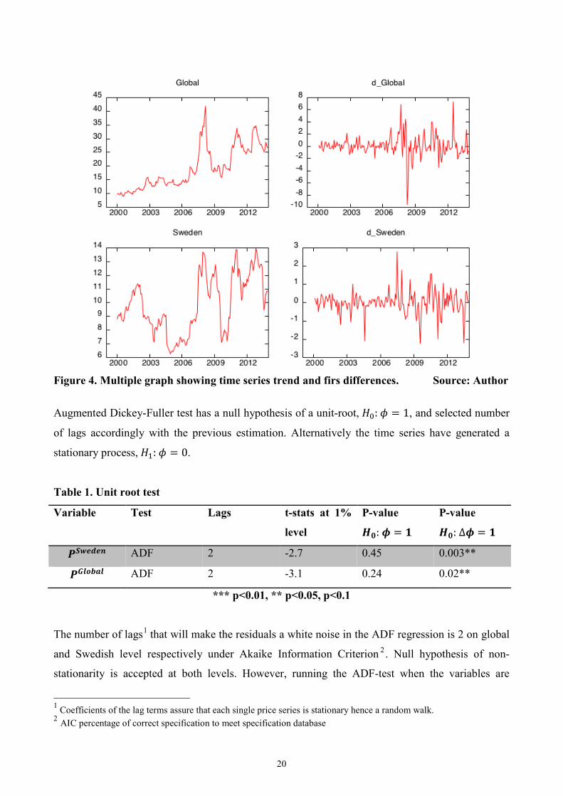
Figure 4. Multiple graph showing time series trend and firs differences. Source: Author

Augmented Dickey-Fuller test has a null hypothesis of a unit-root, 𝐻0: 𝜙 = 1, and selected number

of lags accordingly with the previous estimation. Alternatively the time series have generated a

stationary process, 𝐻1: 𝜙 = 0.

Table 1. Unit root test

Variable Test Lags t-stats at 1%

level

P-value

𝑯𝟎: 𝝓 = 𝟏

P-value

𝑯𝟎: ∆𝝓 = 𝟏

𝑷𝑺𝒘𝒆𝒅𝒆𝒏 ADF 2 -2.7 0.45 0.003**

𝑷𝑮𝒍𝒐𝒃𝒂𝒍 ADF 2 -3.1 0.24 0.02**

*** p<0.01, ** p<0.05, p<0.1

The number of lags1 that will make the residuals a white noise in the ADF regression is 2 on global

and Swedish level respectively under Akaike Information Criterion 2. Null hypothesis of non-

stationarity is accepted at both levels. However, running the ADF-test when the variables are

1 Coefficients of the lag terms assure that each single price series is stationary hence a random walk. 2 AIC percentage of correct specification to meet specification database

20

differentiated the result show strong rejection of the null hypothesis thus the variables have become

stationary.

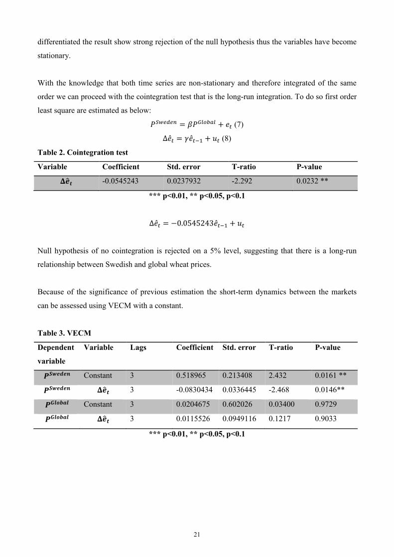
With the knowledge that both time series are non-stationary and therefore integrated of the same

order we can proceed with the cointegration test that is the long-run integration. To do so first order

least square are estimated as below:

𝑃𝑆𝑤𝑒𝑑𝑒𝑛 = 𝛽𝑃𝐺𝑙𝑜𝑏𝑎𝑙 + 𝑒𝑡 (7)

Δ�̂�𝑡 = 𝛾�̂�𝑡−1 + 𝑢𝑡 (8)

Table 2. Cointegration test

Variable Coefficient Std. error T-ratio P-value

𝚫𝒆�𝒕 -0.0545243 0.0237932 -2.292 0.0232 **

*** p<0.01, ** p<0.05, p<0.1

Δ�̂�𝑡 = −0.0545243�̂�𝑡−1 + 𝑢𝑡

Null hypothesis of no cointegration is rejected on a 5% level, suggesting that there is a long-run

relationship between Swedish and global wheat prices.

Because of the significance of previous estimation the short-term dynamics between the markets

can be assessed using VECM with a constant.

Table 3. VECM

Dependent

variable

Variable Lags Coefficient Std. error T-ratio P-value

𝑷𝑺𝒘𝒆𝒅𝒆𝒏 Constant 3 0.518965 0.213408 2.432 0.0161 **

𝑷𝑺𝒘𝒆𝒅𝒆𝒏 𝚫𝒆�𝒕 3 -0.0830434 0.0336445 -2.468 0.0146**

𝑷𝑮𝒍𝒐𝒃𝒂𝒍 Constant 3 0.0204675 0.602026 0.03400 0.9729

𝑷𝑮𝒍𝒐𝒃𝒂𝒍 𝚫𝒆�𝒕 3 0.0115526 0.0949116 0.1217 0.9033

*** p<0.01, ** p<0.05, p<0.1

21

The chosen number of lags for the final model is three due to the Durbin Watson statistics3. Sweden

has a negative adjustment coefficient (-0.08) of the error correction term and is significant at 5%

level (-2.46). The global market does however not respond to disequilibrium between the two

markets due to insignificant t-statistics (0.12). It indicates that Swedish wheat prices are responding

to a change of global wheat prices. Because the adjustment coefficient is negative Sweden is

catching up with price changes on the Global market. Wheat production on Swedish level is

dependent on wheat production globally in the short-run but not vice versa.

Δ𝑃𝑡𝑆𝑤𝑒𝑑𝑒𝑛 = 0.518965(2.432) +

−0.0830434�̂�𝑡−1(−2.468) (9)

Δ𝑃𝑡𝐺𝑙𝑜𝑏𝑎𝑙 = 0.0204675(0.03400) + 0.0115526�̂�𝑡−1

(0.1217) (10)

The two estimates of the error correction model (9) and (10) show the adjustment process to a

temporary disequilibrium.

5.4. Sensitivity analysis

The estimation procedure resulted in many weaknesses due to the sensitivity of the test. To begin

with the selected lag length from the ADF-test was rather suboptimal because of the weak Durbin

Watson statistics in the VECM. On the other hand only one lag was enough to distinguish a

temporary disequilibrium when Sweden being the dependent variable. Subsequently the

cointegration test had to include a constant or the OLS regression would be spurious and show

opposite result than expected. Moreover the Swedish wheat market did not respond at all to shocks

from disequilibrium on the world market. When including an intercept thus a constant to the OLS

regression for short-term dynamics the result turned out logical. Because prices are the only

estimates in the model, other factors are expected to end up in the intercept thus including a

constant is necessary. At last the results turned out to have significant and appealing estimates. The

concluding outcome is then valid and appropriate for analysing integrated markets.

3 Durbin Watson tests for autocorrelation in the residuals hence a value of 2 means no autocorrelation.

22

6 Results The final results are described in this chapter followed by an analysis. A reflection of the method is

presented and finally the conclusion of the research. 6.1. Results and analysis

The final result turned out robust and coherent with my expectations. With that said the two markets

are integrated and a wheat prices are transmitted from global to Swedish wheat market. Prices are

transmitted in the long run but only the Swedish wheat market responds to disequilibrium in the

short run. A prevailing long-run relationship, as indicated from the cointegration test, proves that

Swedish farmers are supposed to catch up with changes on the world market. Referring to the

literature review the grain market is today a part of the equity market where speculations are

important, when for instance the market experience a shortage hence augmented price fluctuations.

Figure 5 is illustrating price trends on the wheat market with monthly prices from year 2000 to 2013.

Figure 5. Wheat nominal price trends in Sweden and globally. Source: Author

As we can see the global prices are both higher and fluctuating more than on the Swedish market.

The graph is also indicating on a quite independent price relationship except from the beginning of

the sample period, suggestion a weak price transmission. Globally the prices have a stronger

upward trend and reached the highest value, 41,96$/kg, in connection with the food price spike.

Sweden only grasped a number of 13,67$/kg thus being more isolated from the global volatility.

Since the last two decades the Swedish wheat market is more exposed to the global market then

0

5

10

15

20

25

30

35

40

45

2000

M01

2000

M09

2000

M17

2000

M25

2000

M33

2000

M41

2000

M49

2000

M57

2000

M65

2006

M01

2006

M09

2007

M05

2008

M01

2008

M09

2009

M05

2010

M01

2010

M09

2011

M05

2012

M01

2012

M09

2013

M05

Sweden

Global

23

before the adaption of CAP. On the other hand CAP secure its members’ food security, health,

animal welfare and so on, by implementing tariffs and quotas that create market distortion, thereof

an explanation why Swedish market has been experiencing a moderate volatility and being “isolated”

from the spikes on global level.

Unluckily crop yield have not been the best in recent years including Sweden. Consequently

changes in exogenous variables such as income and inputs have created distortion to “wheat

equilibrium” where prices and quantities are holding constant. Balanced wheat equilibrium happens

when supply and demand match and the market is not troubled by exogenous variables.

Furthermore external influences are not captured in the econometric modelling though they are

important factors to understand the adjustment process back to equilibrium denoted by the short-

term relationship in the VECM. Because Sweden is a small price taking country changes in

Swedish wheat prices are not influencing on global wheat prices accordingly with the VECM result.

Policy reforms have eased trade barriers and Sweden is today an open small economy protected by

the European Union. Not only have Sweden’s trade barriers been reduced to the surrounding world,

but also in other countries thanks to organizations like WTO and CAP, in hope of more efficient

allocations of agricultural products. A competitive world market is growing, markets becoming

more integrated and price transmissions more common among homogenous products.

Furthermore Swedes are becoming more environmental friendly and shift oil usage to biofuels. The

domestic demand for wheat is increasing as well as in the rest of the world. Industrial countries like

Sweden demand wheat for biofuels while developing countries with growing middle classes

consume more animal products hence livestock consumes wheat based feed. Consequently the

Swedish Government seeks to increase the integration for the ethanol market of what would also be

consistent with the overall goals of the Swedish government, to preserve and improve the national

environment. However biofuel production will suffer if wheat price remain high, but also trade

barriers are contributing to a high price and therefore limiting the trade of wheat. As a result a high

wheat price and trade distortions are contradicting to the worldwide environmental goals, which is

to reduce greenhouse gas emissions, if the ethanol industry suffers. If then a wheat producing

country is troubled with poor harvest like recently in Australia or because of the agitation in

Ukraine, the demand will increase in other regions and create a more volatile climate. Due to varied

circumstances in other countries like drought or improving lifestyles in China and Kazakhstan the

Swedish wheat price will subsequently follow.

24

Because of the international trend of organically produced food, Swedish wheat is demanded and

exported more to the international market. But that does not mean that Sweden also would import

more wheat because of the benefits of trade. The reason is the increasing popularity of locally

produced food to reduce emissions and avoid pesticides. Accordingly wheat is not a perfectly

homogenous commodity, which is contributing to a less integrated wheat market thus price

transmission. With that said the quality of wheat is varying, resulting to an imperfect substitute

between the two markets studied in the research.

6.2. Reflections on the method

Price transmission mechanisms within a dynamic regression model are often observed with ECM.

There are of course many reasons for this although the model has its limitations. First of all it has

good economic implications when studying the correction from disequilibrium from previous

period. Secondly, because time series are often non-stationary the ECM is explicated in terms of

first differences, which eliminates the problem of spurious regression. The third advantage is

explained by the ease of assessing ECM both to general and specific approaches in econometric

modelling. Lastly, the most important characteristic is that the disequilibrium error term is in fact

stationary (in line with the cointegration theory). It induces important implications such that the

cointegration processes imply a kind of adjustment that in the long-run prevent errors from

becoming larger (Asteriou & Hall 2011, pp. 359-360). Thus even small deviations from the

equilibrium will result in an adjustment process on each market.

Drawback with the method is that it ignores transaction cost, which may lead to biased results. The

assumption of two markets being fully integrated is not realistic due to obstruction of transaction

cost. Obviously transportation cost and other hindrances will limit the transmission of price shocks

below a critical level. Consequently a perfect price adjustment will not occur because potential

gains from trade cannot offset trade barriers (Meyer 2004).

As previously noted VECM help forecast variables that are cointegrated, and possibly other related

variables. However, the same stochastic trend is required for cointegration. VECM will be

incorrectly modelled if the variables are no cointegrated, and will result in poor forecast

performance (Stock & Watson 2007).

25

Additionally the frequency of the data can be taken in consideration. In this research monthly data

is used to measure the dynamic price relationship. Von Cramon-Taubadel and Loy (1996) call the

attention to data regularity that exceeds the frequency of the adjustment process due to for instance

arbitrage transaction that belong and interfere price transmission in integrated markets. The data

frequency will of course depend on the characteristics of the market and products to avoid

misinterpretation of the empirical study (Meyer & Cramon-Taubadel 2004).

6.2. Conclusion To conclude the wheat markets are integrated because they share common characteristics like trade.

Due to several trade barriers the markets are not fully integrated and have a strong interdependence

among prices. Eliminating trade distortions would create a smoother price transmission and induce

a more efficient coupled market and less deadweight losses thus welfare gains. Food wise wheat is

perceived as an imperfect substitute on the world market that restricts integration. However the

Swedish government encourage trade of wheat for biofuel production to reduce greenhouse gas

emission. In the long run the integration is predicted to increase because of CAP reforms, increased

demand and production of biofuels in industrial counties as well as a growing demand in

developing countries. By knowing the extent and speed of which the global wheat prices are

transmitted to Swedish wheat prices will help farmers making rational decision regarding

production and sales, banks when specifying contracts to secure farmers revenue and the

government when designing policy agreements with the European Union. The research can be

developed with threshold- and asymmetric cointegration models to get more sophisticated

representations of how wheat prices respond to disequilibrium in the short run and adjust to their

long run equilibrium. However the absence of data on trade distortions remains an unsolvable

problem.

26

References Articles Acosta, A. (2012). Measuring spatial transmission of white maize prices between South Africa and Mozambique: An asymmetric error correction model approach. African Journal of Agricultural and Resource Economics, 7(1), 1-13. Balcombe, K., Bailey, A., & Brooks, J. (2007). Threshold effects in price transmission: the case of Brazilian wheat, maize, and soya prices. American Journal of Agricultural Economics, 89(2), 308-323. Cramon‐Taubadel, S., & Loy, J. P. (1996). Price asymmetry in the international wheat market: Comment. Canadian Journal of Agricultural Economics/Revue canadienne d'agroeconomie, 44(3), 311-317. Fackler, P. L., & Goodwin, B. K. (2001). Spatial price analysis. Handbook of agricultural economics, 1, 971-1024. Gilbert, C. L., & Morgan, C. W. (2010). Food price volatility. Philosophical Transactions of the Royal Society B: Biological Sciences, 365(1554), 3023-3034. Headey, D. (2011). Rethinking the global food crisis: The role of trade shocks. Food Policy, 36(2), 136-146. Johansen, S. (1988). Statistical analysis of cointegration vectors. Journal of economic dynamics and control, 12(2), 231-254. Karantininis, K., Katrakylidis, K., & Persson, M. (2011, August). Price transmission in the swedish pork chain: Asymmetric nonlinear ARDL. In EAAE 2011 Congress, Change and Uncertainty Challenges for Agriculture, Food and Natural Resources. Krueger, A. O., Schiff, M., & Valdés, A. (1988). Agricultural incentives in developing countries: Measuring the effect of sectoral and economywide policies. The World Bank Economic Review, 2(3), 255-271. Listorti, G., & Esposti, R. (2012). Horizontal price transmission in agricultural markets: Fundamental concepts and open empirical issues. Bio-based and Applied Economics, 1(1), 81-108. Meyer, J. (2004). Measuring market integration in the presence of transaction costs–a threshold vector error correction approach. Agricultural Economics, 31(2‐3), 327-334. Meyer, J., & Cramon‐Taubadel, S. (2004). Asymmetric price transmission: a survey. Journal of agricultural economics, 55(3), 581-611. Michaelowa, A., Stronzik, M., Eckermann, F., & Hunt, A. (2003). Transaction costs of the Kyoto Mechanisms. Climate policy, 3(3), 261-278. Mohanty, S., Peterson, E., & Kruse, N. C. (1995). Price asymmetry in the international wheat market. Canadian Journal of Agricultural Economics/Revue canadienne d'agroeconomie, 43(3), 355-366.

27

Ng, S., & Perron, P. (2001). Lag length selection and the construction of unit root tests with good size and power. Econometrica, 69(6), 1519-1554. Sanjuán, A. I., & Gil, J. M. (2001). Price transmission analysis: a flexible methodological approach applied to European pork and lamb markets. Applied Economics, 33(1), 123-131. Sjö, B. (2008). Testing for unit roots and cointegration. Nationalekonomiska institutionen, Lindköpings Universitet. Turunen-Red, A. H., & Woodland, A. D. (1995). International Trade Policy Reforms and their Simulation. REVUE SUISSE D ECONOMIE POLITIQUE ET DE STATISTIQUE, 131, 389-418. Books Asteriou, D., & Hall, S.G. (2011). Applied Econometrics. 2. ed. Hampshire: Palgrave Macmillan. CAP (2012). A partnership between Europe and Farmers. Luxemburg: Publications Office of the European Union. Cottrell, A., & Lucchetti, R. (2012). Gretl user’s guide. Distributed with the Gretl library. Gujarati, D.N. (2004). Basic Econometrics. 4. ed. New York: McGraw-Hill. Perloff, J.M. (2007). Microeconomics Theory and Applications with Calculus. 1. ed. Boston: Pearson/Addison Wesley. Rapsomanikis, G., Hallam, D., & Conforti, P. (2006). Market integration and price transmission in selected food and cash crop markets of developing countries: review and applications. Agricultural Commodity Markets and Trade: New Approaches to Analysing Market Structure and Instability. FAO, 187-217. Stock, H. J., & Watson, W.M. (2007). Introduction to Econometrics, pp. 656-658. Wooldrige, J.M. (2006). Introductory Econometrics. 4. ed. Mason: Macmillan Publishing Solutions. Internets source Agricultural Market Information System. (2014). Prices and price volatility. http://www.amis-outlook.org/index.php?id=40255#.U5ZSVVwYVDs [2014-03-09].

European Union. (2011-05-06). Single Farm Payment. http://europa.eu/legislation_summaries/agriculture/general_framework/ag0003_en.htm [2014-03-10]. FAO - Food and Agriculture Organization of the United Nations. (2014-03-10). Price volatility in agricultural markets. http://www.fao.org/economic/est/issues/volatility/en/#.UyoERFz8BDt [2014-03-10]. Handelsbanken. (2014-01-01). Råvarumarknad. http://www.handelsbanken.se/shb/INeT/IStartSv.nsf/FrameSet?OpenView&amp;iddef=skoglantbruk&amp;navid=Z2_Skogochlantbruk&amp;sa=/shb/INeT/ICentSv.nsf/Default/q1950EF87A1C1F48EC12573E600377EE6 [2014-03-10].

28

Regeringskansliet. (2014-02-03). Reform av den gemensamma jordbrukspolitiken. http://www.regeringen.se/sb/d/6376/a/57962 [2014-03-09] Stata. (2013-01-01). Vec intro – Introduction to vector error- correction model. http://www.stata.com/manuals13/tsvecintro.pdf [2014-03-10]. Unted Nations. Sweden Agriculture. http://www.un.org/esa/agenda21/natlinfo/countr/sweden/agriculture.pdf [2014-03-10]. World Bank (2014-04-01). Overview of Commodity Markets. http://econ.worldbank.org/WBSITE/EXTERNAL/EXTDEC/EXTDECPROSPECTS/0,,contentMDK:21574907~menuPK:7859231~pagePK:64165401~piPK:64165026~theSitePK:476883,00.html [2014-04-13]. Newspapers Butikstrender. (2014-03-04). Spannmålspriser stiger på grund av Ukrainakrisen. http://www.butikstrender.se/spannmalspriser-stiger-pa-grund-av-ukrainakrisen/ [2014-05-01]. Douglasdotter, S. (2013-07-05). Lågt vetepris med hopp om bra skörd. Available at: http://www.trelleborgsallehanda.se/trelleborg/article1922936/Lagt-vetepris-men-hopp-om-bra-skord.html [2014-05-01]. Reports Conforti, P. (2004). Price transmission in selected agricultural markets. FAO Commodity and Trade Policy Research Working Paper, 7. Dawe, D. (2008). Have recent increases in international cereal prices been transmitted to domestic economies. The experience in seven large Asian countries. FAO-ESA Working Paper, (08-03). Hassouneh, I., von Cramon-Taubadel, S., Serra, T., & Gil, J. M. (2012). Recent developments in the econometric analysis of price transmission (No. 2). Working paper. High Level Panel of Experts (2011). Price Volatility in Food and Agricultural Markets: Policy Responses. Food and Agricultural Organization. Lee, H. H., & Park, C. Y. (2013). International Transmission of Food Prices and Volatilities: A Panel Analysis. Asian Development Bank Economics Working Paper Series, (373). Minot, N. (2011). Transmission of world food price changes to markets in Sub-Saharan Africa. Washington, IFPRI, 34. Schnepf, R. (2008). High Agricultural Commodity Prices: What Are the Issues?. Library of Congress, Congressional Research Service. Tarighi, M. (2005). Svenskt jordbruk under 10 år i EU. (Statistikrapport 2005:5). Statens Jordbruksverk. http://www.jordbruksverket.se/webdav/files/SJV/Amnesomraden/Statistik,%20fakta/Annan%20statistik/Statistikrapport/20055/20055_ikortadrag.htm [2014-03-10].

29

Thompson, S. R., & Bohl, M. T. (1999). International wheat price transmission and CAP reform. In 1999 Annual meeting, August 8-11, Nashville, TN (No. 21705). American Agricultural Economics Association (New Name 2008: Agricultural and Applied Economics Association). Phamplets Enhäll, J. (2013). Prisindex och priser på livsmedelsområdet. (JO1010) Jönköping: Jordbruksverket. Jordbruksverket (2012). Höga spannmålspriser på världsmarknaden. (På tal om jordbruk – fördjupning om aktuella frågor) Jönköping: Jordbruksverket. Jordbruksverket (2009). Facts about Swedish Agriculture. (OVR2GB) Jönköping: Jordbruksverket. http://www2.jordbruksverket.se/webdav/files/SJV/trycksaker/Pdf_ovrigt/ovr2gb.pdf

Programs Excel Microsoft Office 2011 Gretl Version gretl-1.9.14.exe Theses Johansson, C,. Magnusson, M,. Säfström, M,. Vågesjö, V,. Åkesson, E. (2014) Bonden, börsklippare eller bidragstagare? (Unpublished). Thesis. Swedish University of Agricultural Sciences. Sharp, G. D. (2010). Lag length selection for vector error correction models (Doctoral dissertation, Rhodes University).

30