15-09 | May 13, 2015

The Influence of Systemic Importance Indicators on Banks’ Credit Default Swap Spreads

Jill Cetina Office of Financial Research Jill.Cetina@treasury.gov

Bert Loudis Office of Financial Research Bert.Loudis@treasury.gov

The Office of Financial Research (OFR) Working Paper Series allows members of the OFR staff and their coauthors to disseminate preliminary research findings in a format intended to generate discussion and critical comments. Papers in the OFR Working Paper Series are works in progress and subject to revision. Views and opinions expressed are those of the authors and do not necessarily represent official positions or policy of the OFR or Treasury. Comments and suggestions for improvements are welcome and should be directed to the authors. OFR working papers may be quoted without additional permission.

OFR Working Paper

May 2015

The Influence of Systemic Importance Indicators on Banks’ Credit Default Swap Spreads

Jill Cetina

Bert Loudis

Abstract This paper examines the relationship between banks’ observed credit default swap (CDS) spreads and possible measures of systemic importance. We use five-year CDS spreads from Markit with an international sample of 71 banks to investigate whether market participants are giving them a discount on borrowing costs based on the expectation that governments would consider them “too big to fail.” We find a consistent, statistically significant negative relationship between five-year CDS spreads and nine different systemic importance indicators using a generalized least squares (GLS) model. The paper finds that banks perceived as too big to fail have CDS spreads 44 to 80 basis points lower than other banks, depending on the asset-size threshold and controls used. Additionally, the study suggests market participants pay more attention to asset size than to a more complex measure, such as designation as a globally systemically important bank (G-SIB), that includes additional factors, such as substitutability and interconnectedness. Lastly, the model suggests that asset size acts as a threshold effect, rather than a continuous effect with the best fitting models using asset-size thresholds of $50 billion to $150 billion. Keywords: Banking, too big to fail, size effect, heightened prudential regulation JEL classifications: G01, G21, G22, G24, G28. Jill Cetina (Jill.Cetina@treasury.gov) and Bert Loudis (Bert.Loudis@treasury.gov) are at the Office of Financial Research. The views expressed in this paper are those of the authors alone and do not necessarily reflect those of the Office of Financial Research. We thank Greg Feldberg (OFR), Paul Glasserman (OFR), Benjamin Kay (OFR), Kevin Sheppard (OFR), and Michael Wedow (European Central Bank) for useful comments and suggestions. The authors take responsibility for any errors and welcome comments and suggestions.

Introduction/Motivation

This paper contributes to the discussion of whether large banks are subject to adequate market

discipline or enjoy a “too-big-to-fail” subsidy in credit markets as a result of perceptions of potential

government support. During the most recent financial crisis and in several prior episodes, the U.S. and

other governments have rescued large financial institutions to avoid the financial instability they feared

would result from the failure of those firms. Market participants may continue to evaluate certain large

financial institutions based on the belief that the government would provide support to those

institutions in a crisis, as opposed to evaluating them on the basis of their stand-alone credit risk.

A number of previous studies have used market data to evaluate creditors’ perceptions that a

company is too big to fail. This paper uses credit default swap (CDS) data. Arguably, this is a more

transparent metric of the credit spreads banks face than deposit costs (see Jacewitz and Pogach, 2013 or

Bassett, 2014), which can have fees or other terms that complicate cross-bank comparisons, or bond

spreads (Santos, 2013 and GAO, 2014), which often contain call provisions. In theory, if market

participants deemed a large bank too big to fail, the bank’s CDS spread would trade tighter than

suggested by its fundamental credit risk. The bank would, as a result, experience lower CDS spreads than

financial institutions market participants did not view as too big to fail.

Efforts to identify the possible impact of the too-big–to-fail perception on banks’ borrowing

costs face several challenges. Borrowing costs reflect idiosyncratic credit risk of individual banks and

liquidity differences in firms’ borrowings.

Volz et al. (2011) use CDS data from Bloomberg for an international sample of 91 banks,

including U.S. banks, coupled with expected default frequencies from Moody’s KMV (now Moody’s

Credit Edge) data to control for credit risk. Volz et al. control for liquidity differences using bid-ask

spreads. They examine the impact of size, measured as market capitalization plus the book value of

liabilities and data on total assets and find evidence consistent with a too-big-to-fail subsidy. Although

1

the authors consider multiple measures of size and data providers, they only consider asset size as a

linear variable and do not examine asset-size thresholds. This paper, on the other hand, uses dummy

variables at various asset size cut-offs and compares them with models using different asset size cut-offs

(threshold effects), along with the dollar value of assets (continuous effects).

Ahmed et al. (2014) use CDS data from Markit (the same source for this paper’s CDS data) for a

sample of 20 U.S. banks, as well as U.S. firms from other industries, and control for credit risk using

expected default frequencies from Moody’s Credit Edge and for liquidity using Markit’s CDS depth

measure (one of three CDS liquidity measures rolled into the Markit liquidity score used in this paper).

Markit compiles its CDS data from the single name reference entity of the CDS transaction and creates a

liquidity rating based on factors detailed in the data section of this paper. The authors also make use of

corporate bond data from the Trade Reporting and Compliance Engine (TRACE) reporting system of the

Financial Industry Regulatory Authority to consider too-big-to-fail effects in the pricing of executed bond

trades. For CDS and bonds, the authors consider size as a linear variable, i.e., the log of the asset size of

a firm as opposed to evaluating whether an asset-size threshold effect exists.1 Ahmed et al. offer

economies of scale as an alternative explanation of why a firm’s asset size affects its observed CDS

spreads. Their argument is that larger firms are more profitable and consequently less likely to default.

However, it could be argued that market participants’ view of the benefits of economies of scale on

profitability is already taken into account by Moody’s Credit Edge, the credit control variable that

Ahmed et al. use, since that variable incorporates measures of profitability and also makes use of stock

price data (which presumably would “price-in” such economies of scale).

Previous papers on this subject have sought to measure time-variation in large banks’ funding

advantages or to quantify the value of the taxpayer subsidy. This paper takes a different approach. We

1 Additionally, expected default frequency (EDF) has a nonlinear relationship with observed CDS spreads, making it difficult to draw economic significance from the model’s coefficients. For example, industries with a low median EDF may have observed CDS spreads that are less affected by a small change in EDF when compared to industries with a higher median EDF. According to the paper, the mean EDF for banks in the sample is the fourth highest of the 14 industries considered.

2

seek to identify where a possible too-big-to-fail effect for banks may be most in evidence by testing

alternative specifications of size and systemic importance. Specifically, we consider whether market

participants allow firms to borrow at a lower cost based on various asset-size thresholds or whether

those firms have been designated by the Basel Committee on Banking Supervision as globally

systemically important banks (or G-SIBs).2 We focus on asset-size thresholds and the G-SIB designation

because regulators have used both types of measures to set heightened levels of prudential regulation.

The paper approaches the analysis in two steps.

First, the paper tests two different alternative controls for credit risk before considering

whether size appears to influence a bank’s CDS spread. Each of the credit control variables is commonly

used by market participants. Several papers use Moody’s Credit Edge to control for credit risk (Volz et

al., 2011 and Ahmed et al., 2014); other papers use controls for credit risk that reflect the authors’ own

perceptions of drivers of credit fundamentals (GAO, 2014). This paper selects the best fitting commercial

credit model from two alternative models and then approaches the too-big-to-fail question.

With regards to controls for liquidity, papers use different control variables depending on the

type of bank liability they are assessing. Papers considering deposits use deposit volumes while papers

evaluating bond spreads use bid-ask spreads (GAO, Santos) to control for differences in liquidity across

banks’ liabilities. Other papers on CDS have used bid-ask spreads (Volz) or depth, i.e., the number of

dealers quoting (Ahmed). This paper uses Markit’s CDS liquidity score, which is a multifaceted measure

that reflects: 1) the freshness of the quote, 2) depth of the market, and 3) the bid-ask spread. These

refinements still yield results consistent with a number of other studies’ findings that suggest a possible

funding advantage for large banks.

The too-big-to-fail subsidy may be relevant to the policy discussion on appropriate asset-size

thresholds for heightened prudential regulation. Since the financial crisis of 2007-09, large banks have

2 See OFR Brief “Systemic Importance Indicators for 33 U.S. Bank Holding Companies: An Overview of Recent Data” for a discussion of the BCBS G-SIB methodology.

3

become subject to heightened prudential regulation and oversight both domestically and

internationally. The Dodd-Frank Wall Street Reform and Consumer Protection Act introduced thresholds

for prudential regulation for U.S. banks. Section 165 of the Act requires that "in order to prevent or

mitigate risks to the financial stability of the United States," the Federal Reserve establish for all bank

holding companies with at least $50 billion in assets prudential standards that "are more stringent" than

generally applicable standards and that "increase in stringency" be based on a variety of factors related

to the systemic importance of these institutions. Among other things, the Dodd-Frank Act also requires

that banks with assets greater than $50 billion be subject to ex-post assessments in the event of

taxpayer losses as a result of resolution of a firm under Title II of the Act. After the failures or near-

failures of many large institutions during the financial crisis, legislation and regulation sought to make

larger firms more safe and sound through heightened prudential standards, including higher capital and

liquidity requirements. The higher standards attempt to ensure that these companies have sufficient

capital and liquidity to weather a crisis, and they seek to promote market discipline by making it less

likely that a large firm would need to be rescued. Under the Dodd-Frank Act, supervisory standards

begin to increase at $50 billion in assets and become significantly more rigorous as companies become

larger and more complex.

Based on analysis of market pricing, market participants appear to be offering cheaper funding

to banks with assets above a certain threshold, which could encourage greater risk taking among these

firms. We believe that this paper is unique in offering an analytic contribution to the policy discussion of

the appropriate cut-off for heightened prudential regulation as it considers multiple asset-size

thresholds and finds that using asset-size thresholds in the $50 billion to $150 billion range have the

largest coefficients and best model fit for a too-big-to-fail effect. By contrast, models with asset-size

thresholds at $200 billion or above are less effective at explaining banks’ CDS spreads. Prior work in this

area has considered too big to fail only as a linear function of bank size, but this paper explores too big

4

to fail as a linear function and a threshold effect. We recognize that CDS spreads are but one way of

measuring the too-big-to-fail subsidy and hope that this paper inspires further analytic work on where

the too-big-to-fail threshold seems most material to better inform regulatory policy development.

Although this paper contributes to the discussion of the appropriate cutoff for heightened prudential

regulation of banks, evidence of a too-big-to-fail subsidy is only one of a number of relevant policy

considerations. Other relevant considerations could include the data used in the Basel methodology for

establishing the G-SIB systemic importance scores3, continued rating agency ratings’ uplift for some

large U.S. banks, and how banks look on the basis of various cross sectional systemic risk measures, such

as conditional value at risk or marginal expected shortfall.4

Data Sample The sample consists of 71 banks from North America, Asia, Europe, and Latin America. Twenty-

one of these banks have been designated as G-SIBs by the Basel Committee. Banks were selected solely

based on the availability of their pricing and transaction data in Markit and their financial data in the

two commercial credit model providers we considered, Bloomberg and Moody’s. Only publicly traded

banks are represented in the sample, because the commercial credit models use a Merton type model

to estimate default probability (distance to default) and then implied CDS spreads.5 A Merton model

views a bank’s equity valuation as a call option on the total assets of the firm where the strike price is

equal to its liabilities. These models can only to arrive at default estimates and implied CDS estimates for

publicly traded banks.

The study compares different datasets on a monthly basis from April 2010 to March 2014. This

period was chosen to examine the G-SIB variable as an indicator of too big to fail and to use Markit’s

3 See OFR Brief “Systemic Importance Indicators for 33 U.S. Bank Holding Companies: An Overview of Recent Data.” 4 See OFR working paper “A Survey of Systemic Risk Analytics” for a discussion of these metrics. 5 None of the models use observed CDS spreads as an input to estimate implied CDS spreads.

5

liquidity score for single-name CDS, a metric that began in April 2010. However, not all of the raw data

we used are reported monthly. For daily data, we used the first data point available for the month, since

monthly data generally reflects the first day of the month. For data available only quarterly or

biannually, such as asset size, we repeated the available data for each month in the reported period.

Dependent Variable

Credit Default Swap Spread (y) — These data were retrieved from Markit, are available at a daily

frequency, and are based on a collection of transactions and dealer quotes for the reference entity. The

CDS spreads in this study are based on the single name reference entity of the CDS transaction. The data

are recorded in percentages, so a regression coefficient of 1.30 represents 1.30 percent, or 130 bps.

Five-year CDS spread data was chosen because it is the most liquid of the spread tenors and contains

the most robust data. The CDS contracts are all quoted in U.S. dollars to avoid exchange rate challenges.

Additionally, only spreads on senior CDS were used in this study. Lastly, restructuring clauses were

streamlined by using the prevailing standards established by each country’s regulatory regime. Variation

in restructuring clauses is controlled for in the models through right-hand geographic variables. Each of

these restrictions on the data set is meant to reduce the noisiness of the data and isolate the possible

too-big-to-fail variables this paper is interested in investigating.

Independent Variables

G-SIB(0,1), G-SIB(cap add-on) — The global systemically important bank (G-SIB) designation is a label

given by the Financial Stability Board (FSB). Established by the 2009 G-20 summit, the FSB has been

tasked with monitoring the global financial system. The purpose of the G-SIB designation is to increase

oversight of banks deemed systemically important and to provide a transparent, rules-based approach

to determining higher capital adequacy requirements for these firms as part of Basel III. The first official

6

G-SIB list was published in November 2011,6 but there were a number of leaks before that date

including a leak to the Financial Times in November 2009.7 To control for leaks of information, we

decided to use the most recent iteration of the G-SIB list from November 2013 and apply it to the entire

sample ranging back to April 2010. The G-SIB(0,1) variable is a binary indication of G-SIB designation,

while the G-SIB(cap add-on) variable contains data points ranging from 0 to 250 basis points depending

on which G-SIB risk-based capital add-on bucket the entity falls into. The larger the bucket, the greater

the level of required additional capital with G-SIB(cap add-on) with values of 1 representing an

additional 100 basis point requirement for banks’ risk-based capital ratios and values of 4 being

representing an additional 250 basis point requirement for banks’ risk-based capital ratios.

Assets > $50B … Assets > $250B — These asset labels were assigned to explore potential too-big-to-fail

threshold effects. They are binary dummy variables, for example, the “Assets > $50B” assigns a 0 for all

banks with assets equal or less than $50 billion and a 1 to all banks with assets greater than $50 billion.

Data on total assets was gathered from Bloomberg and, for non-U.S. institutions, converted into U.S.

dollars using that period’s exchange rate.

Liquidity Fixed Effects — Markit places a liquidity score on individual CDS contracts on a one-to-five

scale, one being the most liquid. The liquidity score is assigned based on three factors: bid-ask spread,

market depth, and data freshness. Each category has a number of demerits that raise the liquidity score

of the entity. Factor 1 is bid-ask spread with a maximum of five demerits. The tightest bid-ask spreads

have no demerits while the widest spreads have five demerits. Factor 2 is market depth with a

maximum of four demerits. According to Markit, “[d]epth can refer to the number of dealers who are

marking their books in Markit’s end-of day service or those that are actively sending runs, combined

6 See www.financialstabilityboard.org/publications/r_111104bb.pdf 7 See www.ft.com/cms/s/0/df7c3f24-dd19-11de-ad60-00144feabdc0.html#axzz3EGCJrZ9E

7

with the volume of runs being sent. The higher the number of participants quoting or submitting end of

day levels, the more liquid the entity-tier is likely to be.” The final factor, factor 3, is data freshness with

a maximum of two demerits. To calculate demerits, Markit uses a basic equation that takes into account

the time individual contributor prices were last updated. A dummy liquidity score of one to five is then

produced based on the total number of demerits.8 Because liquidity is determined from a demerit

system, it is run as a fixed effect with five different binary liquidity variables using a liquidity score of five

as the base liquidity in the regressions. If a single liquidity variable is significant at the 90 percent

confidence level, then the liquidity effects variable is marked “Yes.”

Geographical Fixed Effects — This consists of binary dummy variables used to control for geopolitical

factors that could potentially influence CDS spreads. For the purposes of this study, North America is the

reference geographical zone. Because of data and sample size restrictions, there are no banks included

from Africa or the Middle East.

Time Fixed Effects — These are a collection of dummy variables meant to control for potential time-

varying risk aversion that could exert a systemic influence on observed CDS spreads. The data covers a

period from April 2010 to March 2014, and each of these years is introduced as a binary variable. If one

of the time variables is statistically significant at the 90 percent confidence level, then time fixed effects

are reported as a “Yes” in the regression results.

Bloomberg five-year estimated CDS spread — This variable is derived from the Bloomberg “DRSK model”

available via the Bloomberg terminal. At its core, the DRSK model uses a Merton methodology to

8 The exact ranges and calculations of demerits and the final liquidity score calculation can be found in the Markit user manual, accessible to subscribers of the database.

8

estimate distance to default and derive estimated CDS spreads from data on a firm’s balance sheet,

share price, and share price volatility. Additional adjustments are made to the classic Merton model to

adapt it to estimating CDS spread. More details can be found in a white paper available to Bloomberg

terminal subscribers.9

Moody’s Credit Edge five-year estimated CDS spread – This variable was obtained from Moody’s Credit

Edge service. It makes use of Moody’s enriched Merton model that considers market-based measures of

leverage and asset volatility in estimating a firm’s CDS spread.

Part 1: Evaluation of Fundamental Models Table 1.1: Part 1 Summary Statistics — Total Sample Size = 38

No. of Banks

Req. Capital Add-Ons

Max Asset Size

Median Asset Size

Min Asset Size

Max CDS Spread

Median CDS Spread

Min CDS Spread

Non-G-SIB

23 0 bps

$934.9 B

$174.8 B

$36.3 B

2,525 bps

129 bps

28 bps

G-SIB 1 & 2 buckets

100 to 150 bps

$2,467.6 B

$1,123.7 B

$73.3 B

592 bps

139 bps

37 bps 12

G-SIB 3 & 4 buckets

200 to 250 bps

$2,585.3 B

$2,269.3 B

$1,864.7 B

348 bps

118 bps

59 bps 3

Total 38 N/A $2,585.3 B $339.9 B $36.3 B 2,525 bps 131 bps 28 bps

Sources: Basel Committee on Banking Supervision and authors’ calculations

The table above outlines some summary statistics for the first part of this analysis. Bank of Nova

Scotia, Bank of NY Mellon, and Wells Fargo rank among the lowest CDS spreads in the sample. The

sample represents a broad range of bank sizes, from asset size of $36 billion to $2.6 trillion. To do a side-

by-side comparison of the fit of the two credit models, we required that data for a given bank must be in

9 See Bloomberg, 2014.

9

the Markit, Bloomberg, and Moody’s databases to be included in the regression in this part of the

analysis. A consequence, however, is a more restricted sample of 38 banks compared to the 71 banks in

part 2 of this paper.

The first test for heteroskedasticity used, the Breusch-Pagan Heteroskedasticity Test, indicated

there was a presence of heteroskedasticity at the 99 percent confidence level. A further investigation,

using the White test with Cameron and Trivedi decompositions, indicated the presence of skewness and

kurtosis in the model at the 99 percent confidence level. For this reason, a standard “ordinary least

squares,” or OLS, regression would not give accurate results. A number of other papers in this literature

make use of standard OLS.

In this section of the paper, two separate methods are used to overcome heteroskedasticity.

The first method adds a robust option to the initial regression. The robust option chosen uses Huber-

White sandwich estimators to estimate standard errors. This is commonly used as a minor correction for

heteroskedasticity by producing estimators for ordinary data using stratified cluster sampling. The

results of the robust regression follow in table 1.2. The regressions were reestimated clustering the

banks by name to check for the presence of auto-correlation. These results are shown in Appendix A and

do not alter the conclusions presented in the main text.

10

Table 1.2: Robust OLS Fundamental Model Comparison Dependent Variable: Markit Five-year CDS

Baseline specification Bloomberg Moody's

Bloomberg five-year estimated CDS spread 0.879***

-0.0334 Moody’s Credit Edge five-year estimated CDS spread 0.963***

-0.0480 Constant 0.335*** 0.313*** -0.348***

-0.1350 -0.0696 -0.1190

Liquidity Fixed Effects Yes Yes Yes Time Fixed Effects Yes No Yes Geographical Fixed Effects Yes No Yes

Observations 1,475 1,475 1,475 R-squared 0.170 0.918 0.696

*** p<0.01, ** p<0.05, * p<0.1

The time and geographical controls vary in significance as the right-hand-side variables are

adjusted while the liquidity control remains constant throughout each regression. Bloomberg and

Moody’s are each significant at the 99 percent level when the basic set of controls is applied. To reveal

which model has the most explanatory power, R-squared is used. In this model, Bloomberg has the most

explanatory power with an R-squared of 91.8 percent while Moody’s has an R-squared of 69.6 percent.

Following is a scatterplot of the relationship between the Markit five-year CDS spread and Bloomberg’s

five-year estimated CDS spread.

11

Graph 1.1: Bloomberg Five-year Estimated CDS Spread vs. Markit Five-year CDS Spread

Graph 1.1 shows there is a clear positive relationship between the Markit five-year CDS spread

and Bloomberg’s five-year estimated CDS spread. This is consistent with the results of the robust OLS

regression shown in table 1.2. The scatterplot also lends evidence toward a heavy and predictable

skewness in the model. For this reason, along with the results of the Breusch-Pagan and White tests, a

generalized least squares regression with a heteroskedastic correction option was used in addition to

the robust OLS regression for this section of the paper. Table 1.3 shows the results of the GLS

regression.

0

5

10

15

20

25

30

35

0 5 10 15 20 25 30

Mar

kit 5

y CD

S sp

d

Bloomberg Five-year Estimated CDS Spread

12

Table 1.3: GLS Fundamental Credit Model Comparison Dependent Variable: Markit Five-year CDS

Baseline specification Bloomberg Moody's

Bloomberg five-year estimated CDS spread 0.850***

-0.0115 Moody’s Credit Edge five-year estimated CDS spread 0. 734***

-0.0204 Constant 0.989*** 0.273*** 0.058

-0.0818 -0.0383 -0.0627

Liquidity Fixed Effects Yes Yes Yes

Time Fixed Effects Yes Yes Yes Geographical Fixed Effects Yes Yes Yes

Observations 1,475 1,475 1,475 Bayesian Information Criterion 6,895 3,479 5,419

*** p<0.01, ** p<0.05, * p<0.1

Bloomberg and Moody’s are each significant at the 99 percent level when the basic set of

controls is applied. To reveal which variable has the most explanatory power in this model, Bayesian

Information Criterion (BIC) is used. BIC uses a likelihood function to determine the strength of a model.

Lower BIC scores indicate a better fit model. To reach a BIC score within the GLS framework, the

heteroskedasticity correction needed to be relaxed and the standard GLS autocorrelation model needed

to be used. The BIC results of the robust OLS regression reinforce the finding that the model using

Bloomberg’s implied CDS spreads has the best fit.

The following graphs visually compare the models over time for two large U.S. banks. The charts

illustrate the results of the GLS regression. The Bloomberg model, for the most part, appears to follow

observed CDS spreads more closely than the Moody’s model. For these reasons, the Bloomberg model is

selected as the fundamental credit control, along with other controls, for the next phase of the analysis.

13

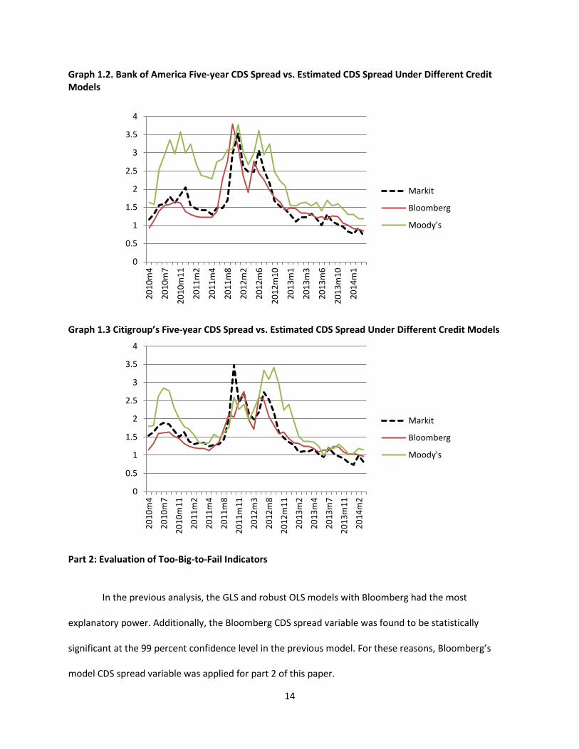
Graph 1.2. Bank of America Five-year CDS Spread vs. Estimated CDS Spread Under Different Credit Models

Graph 1.3 Citigroup’s Five-year CDS Spread vs. Estimated CDS Spread Under Different Credit Models

Part 2: Evaluation of Too-Big-to-Fail Indicators

In the previous analysis, the GLS and robust OLS models with Bloomberg had the most

explanatory power. Additionally, the Bloomberg CDS spread variable was found to be statistically

significant at the 99 percent confidence level in the previous model. For these reasons, Bloomberg’s

model CDS spread variable was applied for part 2 of this paper.

0

0.5

1

1.5

2

2.5

3

3.5

4

2010

m4

2010

m7

2010

m11

2011

m2

2011

m4

2011

m8

2012

m2

2012

m6

2012

m10

2013

m1

2013

m3

2013

m6

2013

m10

2014

m1

Bloomberg

Markit

Moody's

4

0

0.5

1

1.5

2

2.5

3

3.5

2010

m4

2010

m7

2010

m11

2011

m2

2011

m4

2011

m8

2011

m11

2012

m3

2012

m8

2012

m11

2013

m2

2013

m4

2013

m7

2013

m11

2014

m2

Markit

Bloomberg

Moody's

14

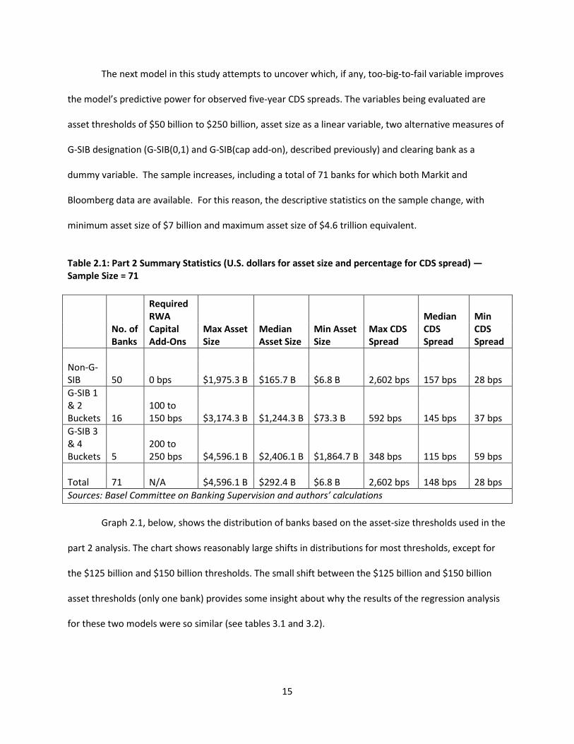
The next model in this study attempts to uncover which, if any, too-big-to-fail variable improves

the model’s predictive power for observed five-year CDS spreads. The variables being evaluated are

asset thresholds of $50 billion to $250 billion, asset size as a linear variable, two alternative measures of

G-SIB designation (G-SIB(0,1) and G-SIB(cap add-on), described previously) and clearing bank as a

dummy variable. The sample increases, including a total of 71 banks for which both Markit and

Bloomberg data are available. For this reason, the descriptive statistics on the sample change, with

minimum asset size of $7 billion and maximum asset size of $4.6 trillion equivalent.

Table 2.1: Part 2 Summary Statistics (U.S. dollars for asset size and percentage for CDS spread) — Sample Size = 71

Required RWA Capital Add-Ons

Max Asset Size

Median Asset Size

Min Asset Size

Max CDS Spread

Median CDS Spread

Min CDS Spread

No. of Banks

Non-G-SIB

0 bps $1,975.3 B

$165.7 B

$6.8 B

2,602 bps

157 bps

28 bps

50

G-SIB 1 & 2 Buckets

100 to 150 bps

$3,174.3 B

$1,244.3 B

$73.3 B

592 bps

145 bps

37 bps

16

G-SIB 3 & 4 Buckets

200 to 250 bps

$4,596.1 B

$2,406.1 B

$1,864.7 B

348 bps

115 bps

59 bps

5

Total

N/A $4,596.1 B $292.4 B $6.8 B 2,602 bps 148 bps 28 bps 71 Sources: Basel Committee on Banking Supervision and authors’ calculations Graph 2.1, below, shows the distribution of banks based on the asset-size thresholds used in the

part 2 analysis. The chart shows reasonably large shifts in distributions for most thresholds, except for

the $125 billion and $150 billion thresholds. The small shift between the $125 billion and $150 billion

asset thresholds (only one bank) provides some insight about why the results of the regression analysis

for these two models were so similar (see tables 3.1 and 3.2).

15

Graph 2.1: Bank Counts Grouped by Asset Size (U.S. dollars) (March 2014)

Tables 3.1 and 3.2 illustrate that, even when using the best credit and liquidity controls

available, a model of banks’ observed five-year CDS spreads is improved by using controls for a possible

too-big-to-fail effect. We consider sequentially nine different possible too-big-to-fail control variables

and each of them is significant at the 99 percent confidence level. The effect persists through different

too-big-to-fail specifications, including the two G-SIB variables described previously, a linear asset size

variable, various asset-size threshold variables, and a clearing bank dummy variable. In every instance,

the too-big-to-fail coefficient is negative, indicating that greater size, being a G-SIB, or being a clearing

bank results in lower observed five-year senior CDS spreads. This is broadly consistent with previous

findings.

Although G-SIB includes asset size, it also reflects other factors, such as interconnectedness. One

might imagine that as a multifaceted measure of systemic importance, it could better capture potential

too-big-to-fail effects. However, when comparing G-SIB variables to the asset size variables, asset size

has substantially greater descriptive power and economic significance than a bank’s G-SIB status. For

0 10 20 30 40 50 60 70

>$250B

>$200B

>$150B

>$125B

>$100B

>$50B

>$0B

Number of Banks

Asse

t Thr

esho

lds

16

example, the coefficient on G-SIB (0,1) is only -15 basis points and the improvement in the BIC is

minimal relative to alternative models that use asset-size thresholds.

When looking at asset size, it appears as if the too-big-to-fail effect is more akin to a threshold

effect than linear. The BIC is lower for nearly every size asset-threshold variable when compared to the

linear size asset variable; which indicates greater descriptive power. Among the asset-size thresholds,

the model suggests that the $50 billion asset threshold is the most economically significant (highest

coefficient) cutoff while the $150 asset threshold is the most statistically significant (lowest BIC). 10

According to this model, banks with assets in excess of $50 billion on average experience a 80 basis

point decline in their CDS spread when controlling for credit fundamentals, liquidity of the CDS and

other factors.11 The $150 billion threshold is significant at the 99 percent level and has the greatest

descriptive power. It should be noted that the $50 billion and $150 billion thresholds have similar

coefficients, while the $125 billion and $150 billion thresholds have similar BICs. The similarity in results

for the $125 billion and $150 billion thresholds is not surprising given the lack of variation in the sample

(depicted in graph 2.1).

Relative to a model with no too-big-to-fail variables, the BIC falls from 9,087 to 8,740 in the

model with the inclusion of the $150 billion threshold (Table 3.1). This implies a substantial

improvement in the model’s performance as a result of the inclusion of this asset-size threshold. The

probability of the original specification being as strong as the specification including the $150 billion

threshold variable is nearly zero (less than 0.0000001 percent). The inclusion of an additional dummy

variable for clearing banks (shown in Table 3.2) adjusts the economic significance of the asset-variable

size slightly, but otherwise maintains the conclusion of Table 3.1. It marginally improves the BIC of the

10 Specifically, the BIC equals -2 * log-likelihood + (# of parameters) x (penalty that depends on the number of data points). When two models have the same number of data points and parameters, the second term will be identical across all models, and so the only difference is -2 * log-likelihood. So half of the BIC difference measures the log-likelihood difference between models, and in a pseudo-Bayesian interpretation the odds of one model being no different than the other, is approximately exp ((BIC_1 – BIC_2)/2). So, the BIC for the asset-size threshold model relative to the log-asset-size model indicates a much better fit of the asset-size threshold model.

17

regression as well. The robust regression in Appendix B checks for autocorrelation in the same fashion as

the previous section of this paper, by clustering based on bank name. Ideally, the model would be

checked using first differences. However, in the sample, bank size is highly persistent and so there is

little time series variation in bank size to identify this effect. In the Appendix B regression, which clusters

based on bank name (autocorrelation check), the $150 billion threshold has the greatest economic and

statistical significance. Another adjustment made by the autocorrelation check model is that the G-SIB

cap add-on variable becomes statistically insignificant.

18

Table 3.1 shows the results of the GLS model using Bloomberg as a credit control variable and exploring a range of alternative variables, including G-SIB and asset size, meant to proxy for a too-big-to-fail effect.

19

Table 3.2 shows the results of the GLS model using Bloomberg as a credit control variable and exploring a range of alternative variables meant to proxy for a too-big-to-fail effect, including a clearing bank dummy variable in addition to G-SIB and asset-size variables explored previously.

20

Conclusion

This paper seeks to use the best available credit and liquidity controls to explain a sample of

international banks’ observed five-year single-name CDS spreads. In this regard, the paper uses both

credit and liquidity control variables not previously used in the literature. Even with these more robust

controls for credit and liquidity fundamentals, the best fit model still would include asset size as an

explanatory variable for banks’ observed CDS spreads. If credit fundamentals and liquidity differences

are properly controlled for, it is not apparent, aside from a too-big-to-fail effect, why the asset size of a

bank would strengthen the model.12

The data suggest that models using nonlinear asset-size thresholds have the most economic and

statistical significance. Banks perceived as too big to fail, based on asset-size thresholds, have CDS

spreads 44 to 80 basis points lower than other banks. The study finds that the econometric models that

use asset thresholds of $50 billion to $150 billion to indicate a too-big-to-fail effect have the best fits

(both via R-squared in the OLS regressions and BIC in the GLS regressions) and largest too-big-to-fail

coefficients (when checked for autocorrelation).

There have been calls from some policymakers to change the $50 billion Dodd-Frank Act

threshold. Heightened prudential regulation for large firms presumably seeks, at least in part, to address

market failure associated with lack of sufficient market discipline arising from investors’ perceptions of

too big to fail. This paper offers an analytic contribution on the question of size thresholds for

heightened prudential regulation of large banks. We recognize that CDS spreads are but one way of

considering this topic – systemic importance data, rating agency ratings uplift, and cross-sectional

systemic risk metrics are other possible approaches.

12 We would anticipate economies of scale to be “priced in” to the equity valuation of large banks and captured in the credit model used in that paper, as well as in the credit model used in this paper’s analysis.

21

References Ahmed, Javed and Anderson, Christopher and Zarutskie, Rebecca, Are Borrowing Costs of Large Financial Firms Unusual?, accessed from SSRN on September 30, 2014. Bassett, W. 2014. Using insured deposits to refine estimates of the large bank funding advantage. Federal Reserve Board working paper. Bisias, D., Flood, M., Lo, A., and Valavanis, S. A Survey of Systemic Risk Analytics, OFR working paper, January 2012. Bloomberg Credit Risk DRSK, Framework, Methodology and Usage, accessed November 2014. Demirguc-Kunt, A., Huizinga, H., 2013. Are banks too-big-to-fail or too-big-to-save? Journal of Banking and Finance 37, pg 875-894. GAO, U.S., 2014. Evidence from the bond market on banks’ “too-big-to-fail” subsidy. GAO 14-621, United States Government Accountability Office Report to Congress. Markit CDS Liquidity User Guide 2014, accessed through the internal OCC Economics database. Jacewitz, S., Pogach, J., 2012. Deposit rate advantages at the largest banks. Working paper available at SSRN. OFR Brief “Systemic Importance Indicators for 33 U.S. Bank Holding Companies: An Overview of Recent Data.” February 2015. Santos, J, 2014. Evidence from the bond market on banks’ “too-big-to-fail” subsidy. Economic Policy Review. Volz, S, Wedow, M, Market discipline and too-big-to fail in the CDS market: Does banks’ size reduce market discipline? Journal of Empirical Finance, Volume 18, Issue 2, March 2011, pg. 195-210.

22

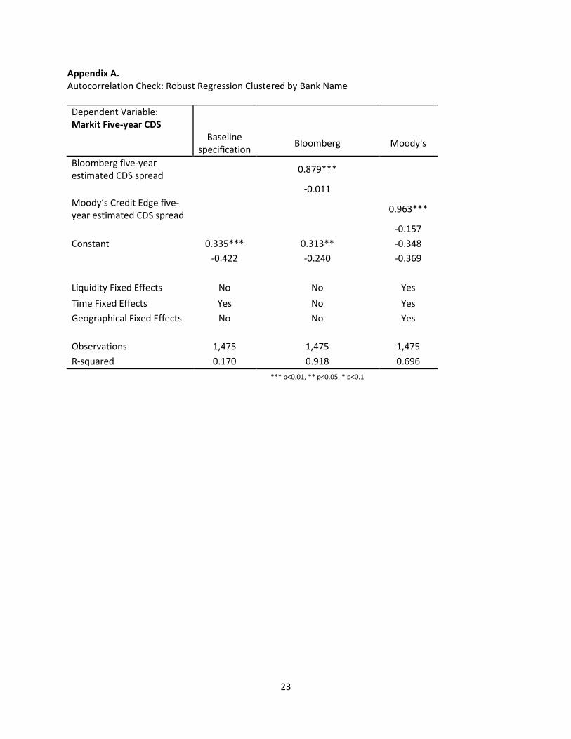
Appendix A. Autocorrelation Check: Robust Regression Clustered by Bank Name Dependent Variable: Markit Five-year CDS

Baseline

specification Bloomberg Moody's

Bloomberg five-year estimated CDS spread 0.879***

-0.011 Moody’s Credit Edge five-year estimated CDS spread 0.963***

-0.157 Constant 0.335*** 0.313** -0.348

-0.422 -0.240 -0.369

Liquidity Fixed Effects No No Yes Time Fixed Effects Yes No Yes Geographical Fixed Effects No No Yes

Observations 1,475 1,475 1,475 R-squared 0.170 0.918 0.696

*** p<0.01, ** p<0.05, * p<0.1

23

Appendix B. Autocorrelation Check: Robust Regression Clustered by Bank Name

24