This paper presents preliminary findings and is being distributed to economists and other interested readers solely to stimulate discussion and elicit comments. The views expressed in this paper are those of the author and are not necessarily reflective of views at the Federal Reserve Bank of New York or the Federal Reserve System. Any errors or omissions are the responsibility of the author.

Federal Reserve Bank of New York Staff Reports

Risk-Neutral Systemic Risk Indicators

Allan M. Malz

Staff Report No. 607 March 2013

Risk-Neutral Systemic Risk Indicators Allan M. Malz Federal Reserve Bank of New York Staff Reports, no. 607 March 2013 JEL classification: G01, G13, G17, G18, G21

Abstract This paper describes a set of indicators of systemic risk computed from current market prices of equity and equity index options. It displays results from a prototype version, computed daily from January 2006 to January 2013. The indicators represent a systemic risk event as the realization of an extreme loss on a portfolio of large-intermediary equities. The technique for computing them combines risk-neutral return distributions with implied return correlations drawn from option prices, tying together the single-firm return distributions via a copula to simulate the joint distribution and thus the financial-sector portfolio return distribution. The indicators can be computed daily using only current market prices; no historical data are involved. They are therefore forward-looking and can exploit all the information impounded in current prices. However, the indicators blend both market expectations and the market’s desire to protect itself against volatility and tail risk, so they cannot be readily decomposed into these two elements. The paper presents evidence that the indicators have some predictive power for systemic risk events and that they can serve as a meaningful market-adjusted point of comparison for fundamentals-based systemic risk indicators. Key words: systemic risk, option pricing, copula methods, risk-neutral distributions, implied correlation _________________

Malz: Federal Reserve Bank of New York (e-mail: allan.malz@ny.frb.org). For their comments, the author thanks Tobias Adrian, Sean Campbell, Ron Feldman, Ken Heinecke, Trish Mosser, Carlo Rosa, and Hao Zhou, as well as seminar participants at the Federal Reserve Banks of New York and San Francisco and the Federal Reserve Board. The views expressed in this paper are those of the author and do not necessarily reflect the position of the Federal Reserve Bank of New York or the Federal Reserve System.

Contents

1 Introduction 1

2 Construction of the risk-neutral indicators 3

2.1 Included firms and data . . . . . . . . . . . . . . . . . . . . . . . . . 3

2.2 Risk-neutral probability distributions . . . . . . . . . . . . . . . . . . 4

2.3 Implied correlations . . . . . . . . . . . . . . . . . . . . . . . . . . . 6

2.4 Computing the indicators via a copula . . . . . . . . . . . . . . . . . 8

3 Indicators of systemic risk 10

3.1 Portfolio systemic risk indicators . . . . . . . . . . . . . . . . . . . . 11

3.2 Probability of systemic risk event conditional on individual firm distress 12

3.3 Probability of firm distress conditional on systemic risk event . . . . . 13

4 Discussion of the results 14

5 Validation and comparison of the results 16

5.1 Option-based indicators and crisis losses . . . . . . . . . . . . . . . . 17

5.2 Option-based indicators and supervisory stress tests . . . . . . . . . . 18

5.3 Option-based indicators and other systemic risk measures . . . . . . . 20

6 Conclusions and issues 20

ii

1 Introduction

This paper describes a set of indicators of systemic risk based on market prices of equity

and equity index options. We display results from a prototype version, computed daily

from January 2006 to January 2013.

The indicators described here are related to the “market-based” metrics described

in recent papers applying financial risk management tools to the measurement of

systemic risk: Segoviano and Goodhart (2009), Acharya, Pedersen, Philippon and

Richardson (2010), Adrian and Brunnermeier (2011), Huang, Zhou and Zhu (2011),

Brownlees and Engle (2011), Gray and Jobst (2011), and Hovakimian, Kane and

Laeven (2012).1

The approaches in these papers have in common the definition of systemic risk as an

extreme loss on a portfolio of assets related to financial intermediaries’ balance sheets.

This definition of systemic risk focuses on the financial health of intermediaries, rather

than on monetary and credit conditions, as the proximate determinant of the likelihood

of a severe crisis.

The systemic risk measures in these papers differ in several key dimensions:

Metric of loss: The metric of loss in this literature is typically a balance-sheet quan-

tity, that is, the firms’ debt securities, as in Huang et al. (2011), the firms’ equity

market value, as in Acharya et al. (2010) and Brownlees and Engle (2011), or

the firms’ asset value, as in Adrian and Brunnermeier (2011). The systemic risk

indicators presented here define a systemic risk event as a large loss in the equity

market capitalization of a portfolio of financial firms.

The metric can also be framed as an insurance premium. Huang et al. (2011)

and Hovakimian et al. (2012) compute the premium cost of insurance against

losses on the aggregate debt of individual intermediaries and of the banking or

financial sector.

Distributional characteristic: The risk of an extreme loss over a specified time hori-

zon can be measured by the probability of occurrence of a loss of given size,

as a quantile of the loss distribution corresponding to a given low probability

(Value-at-Risk, or VaR), or as the expected value of a loss if a given quantile is

exceeded (expected shortfall). VaR and expected shortfall can be expressed in

dollars or as a return. The time horizon, the threshold loss size, and threshold

1See Bisias, Flood, Lo and Valavanis (2012) for a comprehensive survey of the current state of

research on systemic risk measurement. In Bisias et al.’s (2012) main taxonomy of systemic risk

measures, some of the indicators described in this paper would be denoted “forward-looking” or “cross-

sectional.”

1

probability can be varied. The option-based approach described in this paper can

generate all these risk metrics.

Entity and conditioning: The probability, magnitude, or expected value of an ex-

treme loss can be measured for an individual financial intermediary or for a

portfolio of firms, representing the financial system. The metrics can be uncon-

ditional, or conditional on the occurrence an of an extreme loss of an individual

firm. Conversely, the probability, magnitude, or expected value of a firm’s ex-

treme loss can be unconditional, or conditional on the occurrence an of an

extreme loss of the system or portfolio. The approach described in this paper

can generate conditional and unconditional risk metrics at both the firm and

portfolio levels.

Type of data: Systemic risk measures can be computed using historical data on mar-

ket prices and fundamentals, as in Adrian and Brunnermeier (2011), using his-

torical market prices of equity and debt securities issued by the firms, as in

Acharya et al. (2010) and Brownlees and Engle (2011), or using both historical

and current market prices of the firms’ debt and equity issues, or credit default

swaps (CDS), as in Huang et al. (2011). Most historical data on fundamentals

is available at monthly or quarterly frequency.

The approach described here relies only on market data that is available daily.

They can be computed daily using only current market prices of options, equities,

and in a variant of the indicators, CDS; no historical data are involved.

To distinguish this new set of indicators while retaining its association with those

presented in the previous literature, we will denote them as Option-Based Systemic

Expected Shortfall Statistics (OBSESS). In contrast to the papers just cited, OBSESS

are entirely market-based. They are therefore forward-looking, and can exploit all the

information impounded in current prices.

However, they are therefore also risk-neutral and it is worth reiterating the well-known

fact that they are thereby not the same as real-world probabilities, correlations and

quantiles. Rather, they are influenced, perhaps heavily, by risk preferences. Change

in OBSESS can be due to changes in real-world probabilities and correlations, or risk

preferences, or both. OBSESS blend both market expectations and the market’s

desire to protect itself against tail risk, and can’t be easily decomposed into these

two elements. They can therefore best be thought of as benchmarks that translate

current market prices into risk measures, rather than forecasts.

2

2 Construction of the risk-neutral indicators

Our estimation procedure relies on the copula approach, in which a set of simulations

from a multivariate distribution chosen by the modeler is combined with estimates of

the marginal return distributions of the portfolio constituents to arrive at an estimate

of the portfolio return distribution. Copulas are widely used in valuation and risk

modeling of credit portfolios and structured credit products, and are used in several of

the papers just cited. The copula in our application is computed from two estimated

components, the risk-neutral probability distributions of the individual financial firms’

equity returns, and the risk-neutral implied equity return correlation.

There thus three key components in our approach: estimates of individual firms’

equity return distributions, an estimate of the return correlation, and an estimate of

the copula that ties them together. In the implementation described here, we use a

normal copula with a constant pairwise correlation parameter. The marginal return

distributions are estimated as the equity option-based risk-neutral distributions of the

constituents, incorporating additional information in the credit default swap spreads

of the constituents. The normal copula correlation is estimated as the risk-neutral

implied correlation.

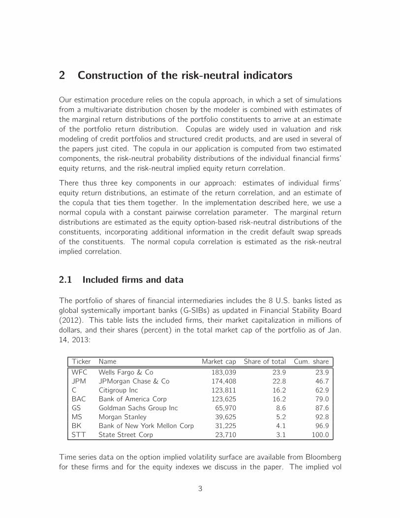
2.1 Included firms and data

The portfolio of shares of financial intermediaries includes the 8 U.S. banks listed as

global systemically important banks (G-SIBs) as updated in Financial Stability Board

(2012). This table lists the included firms, their market capitalization in millions of

dollars, and their shares (percent) in the total market cap of the portfolio as of Jan.

14, 2013:

Ticker Name Market cap Share of total Cum. share

WFC Wells Fargo & Co 183,039 23.9 23.9

JPM JPMorgan Chase & Co 174,408 22.8 46.7

C Citigroup Inc 123,811 16.2 62.9

BAC Bank of America Corp 123,625 16.2 79.0

GS Goldman Sachs Group Inc 65,970 8.6 87.6

MS Morgan Stanley 39,625 5.2 92.8

BK Bank of New York Mellon Corp 31,225 4.1 96.9

STT State Street Corp 23,710 3.1 100.0

Time series data on the option implied volatility surface are available from Bloomberg

for these firms and for the equity indexes we discuss in the paper. The implied vol

3

surfaces are calculated daily by Bloomberg from exchange-traded option data. In this

paper, we use as inputs the Bloomberg volatility smile for options with three months’

remaining maturity. It includes implied vols for exercise prices equal to 80, 90, 95,

97.5, 100, 102.5, 105, 110, and 120 percent of the cash market underlying price,

that is, nine strikes in total. I also rely on Bloomberg for cash market prices, trailing

dividend yields and 3-month U.S. T-bill rates.2

The techniques described in this paper can be carried out for other portfolios chosen

to represent the financial system, provided option data are available, for example, a

portfolio including large non-U.S. banks. In Section 5, for example, we consider the

results for a larger portfolio of U.S. intermediaries that includes the larger regional

banks and some non-banks.

2.2 Risk-neutral probability distributions

The risk-neutral probability distributions of the future market value of each firm or

index can be computed from their equity option prices, together with the current 3-

month T-bill rate and each firm’s dividend yield. The fact that a distribution of future

underlying prices is implied by the current market prices of options with the same

tenor and a range of exercise prices was originally stated by Breeden and Litzenberger

(1978) and Banz and Miller (1978). It can be expressed in terms of puts or calls; the

future value of the rate of change of the put price as the exercise price increases is

equal to the cumulative probability distribution function of the future underlying price.

Letting p(t, τ, X) denote the time-t price of a τ-year put struck at X, r the time-t

τ-year financing rate, and Π(St+τ) the risk-neutral distribution function of the future

asset price St+τ ,

Π(St+τ) = erτ ∂

∂Xp(t, τ, X).

Figlewski (2010) provides some nice intuition for this statement. Consider the increas-

ing value of a put option, for a given current market price of the underlying, as the

exercise price varies from low to high. At very low exercise prices this function has a

slope of zero and at very high ones a slope equal to erτ . As we increase the exercise

price from X to a nearby point X + Δ, the risk-neutral expected future value of the

payoff of the option increases by Δ times the risk-neutral probability Π(X + Δ) that

the option expires in-the-money.

The computation sequence is fairly standard, and is described in greater detail in

Malz (2013). The pros and cons of the choices involved are reviewed in Bliss and

2The option data are retrieved as fields pertaining to the stock or index tickers. The raw data on

which the Bloomberg data is based are displayed, for each firm or index, with the OMON function.

Future work may explore alternative data sources such as OptionMetrics LLC’s Ivy DB.

4

Panigirtzoglou (2002), Jackwerth (2004), and Mandler (2003). In the first step,

as I’ve implemented it for this paper, the Bloomberg implied volatilities are used to

estimate a smooth interpolating function, specifically, a cubic spline with endpoints

clamped so that the slope of the interpolating function is zero beyond the lowest- and

highest-strike options, i.e. those with exercise prices 20 percent above and below the

cash price. The extrapolated volatilities outside the range of observed volatilities are

thus equal to those at the edges of the range.

This approach to interpolation and extrapolation has the virtues that it passes through

all the implied volatilities in the Bloomberg data set, that it is quite smooth, and that

it avoids letting the extreme tail volatilities get very high or low. Extreme volatilities

are not in themselves a problem, but an extremely steep slope of the volatility smile

can violate no-arbitrage restrictions on option prices.3 The interpolation approach

taken here arbitrarily flattens the volatility smile outside the ±20 percent moneynessrange.

In the next step, the interpolated volatility function is substituted into the Black-

Scholes European call option value formula, providing us with the estimated market

value of an option with any stipulated exercise price. The risk-neutral distribution and

density functions, finally, can then be computed by taking differences of option prices.

The differencing interval is set to be large enough to avoid negative densities.

The systemic risk indicators presented here do not crucially depend on this particular

approach to estimating risk-neutral distributions, though the specific numerical results,

of course, do. It would be useful in future work to compare the results when computed

via one of the many alternative approaches to risk-neutral density estimation. Figure 1

displays the resulting risk-neutral distributions for February 11, 2011. The points in

each panel correspond to the moneyness of the option data. All the distributions on

that date are heavily skewed to the left; this is a persistent feature for all 8 firms and

over the entire period covered by the data set.

Figure 2 displays, for each firm, time series of the risk-neutral probability of a loss of 25

percent or more of equity value over the subsequent three months. These probabilities

peaked for all firms, unsurprisingly, at the end of 2008 or the first quarter of 2009.

Sharp increases also took place following the initial Greek bailout request in April 2010,

and particular following the debt-ceiling agreement and resurgence of euro area stress

in July and August 2011. Tail risk has declined for all firms since then, and by early

2013 had fallen nearly, but not quite, to pre-crisis levels.

Expected shortfall at a given confidence level can also be computed for each firm at

each date from the simulated returns. At a 5 percent confidence level, with 10,000

simulations, it is equal to the average of the 500 worst simulated returns. It can be

3See Hodges (1996) and Malz (2013).

5

expressed as a proportional return, or in dollars. We don’t display these results in

the paper. But for all the included firms, measured over the crisis, expected shortfall

expressed in dollars falls rapidly from its peak as large market-value losses were realized,

and rises again from the end of the first quarter of 2009, when values began to recover.

Once a large part of the market cap has been obliterated, less remains to be obliterated

going forward. Expected shortfall expressed in percent, in contrast, remains at its peak

from late 2008 through the first quarter of 2009 for the included firms.

2.3 Implied correlations

A risk-neutral implied return correlation between financial stocks can be estimated from

the implied volatilities of individual stocks in the KBW Bank Sector Index (managed

by Keefe, Bruyette & Woods, Bloomberg ticker BKX), and the implied volatility of

options on the BKX index itself. We obtain an estimate of the constant pairwise

correlation among the constituent stocks that is consistent with the option data.

The constituents of the BKX index are 24 money-center and large regional banks,

weighted by their market capitalization. The BKX constituents overlap with but are

not identical to the list of firms used in estimating OBSESS4. There are no other

indexes of U.S. financial firms for which option-price data are readily available, so we

don’t have the luxury of choosing one that coincides exactly with the set of firms

included in the OBSESS.5 Rather, we use the BKX constituents to obtain a single,

reprsentative implied correlation of financial firms.

The index volatility is

rindex,t =K∑

k

ωktrkt ,

where rindex,t represents the time-t index return, and ωkt and rkt the time-t weights

and returns on the k = 1, . . . , K constituent stocks (with K = 24). Assuming that

the pairwise correlation ρjk,t = ρt , ∀j, k is the same for all the constituents, the indexreturn volatility σindex,t is related to the K volatilities σ

2kt of individual stock returns by

σ2index,t =∑

k

ω2ktσ2kt + 2ρt

∑

k

∑

j<k

ωjtωjtσktσkt .

We know the weights in the index. If we also know the volatilities, we can estimate a

risk-neutral ρt as

ρt =σ2index,t −

∑k ω2ktσ

2kt

2∑k

∑j<k ωjtωjtσktσkt

4GS and MS are not in BKX.5One could, however, compute a version of the OBSESS using the constituents of the BKX index.

6

by substituting the observed at-the-money implied volatilities for the population return

standard deviations. Risk-neutral correlation is high when the index vol is high relative

to the “typical” single-stock vol.

Skintzi and Refenes (2005) describe the empirical characteristics of implied equity

correlation and its efficacy as a forecast of future realized correlation.6 Driessen,

Maenhout and Vilkovn (2009) provide evidence that correlation risk commands a

negative risk premium. That is, financial products such as index options, which have

better payoffs when return correlation increases, are too dear relative to single-stock

options to be fully explained by expected realized volatilities and pairwise correlations.

Buyers of index options are thus paying an insurance or risk premium to sellers.

The correlation risk premium is related to market pricing of idiosyncratic relative to

systematic risk. In a period of stress, the magnitude of this risk premium tends to

increase, as market participants are eager to quickly hedge all long exposures, rather

than specific positions. They therefore seize on index volatilities, which are more liquid

and require fewer trades to get the portfolio covered, leading to an increase in implied

correlation.

Figure 3 displays the time series of bank-sector implied correlation.7 The correlation

has generally been higher, but also more variable, since the onset of the crisis. Like

firms’ tail risk measures, it has recently been declining, but not all the way back to

pre-crisis levels.

However, as noted by Kelly, Lustig and Van Nieuwerburgh (2011), prices of options on

financial firms also reflect implicit public-sector guarantees such as the too-big-to-fail

policy. The perception of such guarantees may have the opposite effect to portfolio

hedging, by increasing the idiosyncratic risk that shareholders of some individual finan-

cial firms will take large losses or be wiped out, even if most firms and the financial

sector as a whole are supported. One could think of this as “Lehman risk.”

The public-sector subsidy or guarantee thus increases the value of options on at least

some individual firms relative to index options, lowering the implied equity correlation.

As seen in Figure 3, bank-sector implied correlation was highest in the early phases

of the financial crisis, but reached a low in the second quarter of 2009, after the full

range of government and Federal Reserve emergency lending programs had been rolled

out.

Other firm-specific and market-based measures of systemic risk use historical rather

than current market data to compute return correlations among firms. For example,

6Earlier studies of option-implied correlation, for example Campa and Chang (1998) and Lopez

and Walter (2000), focused on correlations among U.S. dollar exchange rate pairs implied by prices of

cross-currency options.7A few vol data points are missing for some firms (44 in total). The implied correlation is computed

using all the vols available on a given day.

7

Huang et al. (2011) and Brownlees and Engle (2011) apply Dynamic Conditional

Correlation.8 Adrian and Brunnermeier’s (2011) CoV aR does not compute firms’

pairwise return correlations explicitly. Rather, the interaction between firms is captured

through the estimated relationships or “betas” (a) between firms’ or the portfolio’s

outlier returns and outliers in the factors driving risk and (b) between firms’ and

the portfolio’s outlier returns. By using historical data, these approaches are able

to distinguish the different dependence relations of different pairs of firms, while our

approach is constrained to a single correlation for all pairs of firms.

2.4 Computing the indicators via a copula

The indicators presented in this paper endeavor to capture the interaction between

individual firms and the financial sector, and are computed using a copula. Copula

techniques are useful when we don’t know the joint distribution of a set of random

variables, but believe we possess at least some information about their correlations,

and good information about the marginal distributions. The copula lets us simulate

the joint distribution of the individual firms’ returns given their marginal probability

distributions and an estimate of their return correlation.

Copula techniques were introduced into finance as an approach to modeling of portfolio

credit returns, for which the same problem arises as in our context: good information

on marginal distributions, but limited information on the joint distribution of returns.

An early application was Li (2000).

We use a multivariate normal (Gaussian) copula. This isn’t tantamount to assuming

the equity returns themselves are jointly normally distributed. Rather, the date-t

returns are posited to consistent with

Φ[Φ−1(ut1), . . . ,Φ−1(utN);Rt],

where Φ(x) represents the univariate standard normal cumulative distribution function

and Φ(x;R) the distribution function of a multivariate standard normal with a corre-

lation matrix R. The utn are the probabilities we obtain from the date-t risk-neutral

distributions. The date-t correlation matrix Rt has dimension equal to N, the number

of firms in the portfolio (with N = 8 here). All its off-diagonal elements are set equal

to the risk-neutral implied correlation for that date, as described in the previous sub-

section. The Φ−1(utn) are the “shadow” or latent normal variates that “would havedelivered” the marginal probabilities utn, and it is these that are assumed to be jointly

normal, not the returns themselves.

For each date, the simulation follows these steps:

8See Engle(2002, 2009).

8

• Generate I = 10, 000 simulated values ztin from an N-dimensional multivariatestandard normal with correlation matrix Rt.

• The marginal probability utin = Φ(ztin) of each of the I × N simulated valuesis computed as the value of the univariate cumulative probability function of a

standard normal random variable, taking the simulated value as its argument.

• Each marginal probability utin is then mapped to a corresponding return or equityvalue using the risk-neutral distributions. The corresponding return is that with

a risk-neutral probability equal to the simulated utin = Φ(ztin).9

The result for each date is an I ×N table of I simulated proportional returns on eachof the N stocks. They can be used together with market capitalizations to compute

dollar returns for the firms, which in turn can be added across firms to compute the I

simulations of the portfolio dollar return on each date. A high correlation will fatten

both tails of the portfolio return distribution, since extreme outcomes for individual

firms will have a greater propensity to coincide in each simulation. The OBSESS are

then computed from the quantiles and order statistics of the simulation results of

individual firms and of the portfolio.

The copula approach is consistent with what we think we know, given each day’s

option data, about the marginal distributions and the correlations, but adds to it

enough modeling apparatus to enable us to simulate the joint distribution. The data

don’t prescribe any particular copula. We could, for example, readily substitute a

multivariate Student’s t copula for the multivariate normal to generate the I×N tableof simulated values in the first step of the procedure. In contrast to the normal, the

univariate t distribution has heavy tails, and the multivariate t distribution has positive

coefficients of lower and upper tail dependence.

Simulations using the t copula would therefore likely lead to greater clustering of

extreme outcomes in the simulated returns, and there is empirical evidence that the t

copula better captures the behavior of equity returns than the normal copula.10 But

9An earlier version of this paper incorporated CDS data as follows: If, in a simulation, the marginal

probability is less than or equal to the CDS-based three-month default probability, the equity loss for

that firm in that simulation is 100 percent. The CDS are not essential to the computations. If they

are included, and the default probabilities are high enough, they will fatten the left tails of the firm and

portfolio return distributions by generating a material number of simulations in which there is a 100

percent loss.10Demarta and McNeil (2005) compare the t copula and its tail dependence properties to others,

including the normal. The multivariate t copula is recommended for portfolios with nonlinear risks such

as options by Glasserman, Heidelberger and Shahabuddin (2002). Mashal, Naldi and Zeevi (2003)

present evidence that the t copula is more accurate than the normal for forecasting extreme events.

A (likely) less crucial issue is that the choice of copula is arbitrary. In future work, one could compare

OBSESS computed using a multivariate t distribution with, say, four degrees of freedom, but the same

correlation matrix.

9

the typically rather stout left tails of the individual banks’ risk-neutral distributions,

together with high implied correlations, themselves induce a good deal of clustering of

left-tail outcomes in the simulations.11 Moreover, as we will see below in our discussion

of the results, comovement of variance and correlation premiums, together with the

clustering of left-tail outcomes, make it more difficult to discriminate between results

for different firms.

But the market data themselves do not provide guidance on which copula is appro-

priate, only on the risk-neutral marginal return distributions and return correlations.

The t-copula is infrequently used in practice. Risk management sensitivities based on

the normal copula are routinely computed for standard tranches of credit index default

swaps such as the CDX and iTraxx, and serve a standardization function similar to

that of the Black-Scholes formulas in option markets.

3 Indicators of systemic risk

The risk-neutral systemic risk indicators are computed from the simulated returns.

As with any distribution-based risk measures, the “user” must choose thresholds—

events and quantiles—that define “extremeness.” We define a systemic risk event as

a large loss of equity market value of the portfolio of included firms, specifically, a loss

of x percent in the aggregate market capitalization of the 8 firms, with x set to a

large number: 15, 20 or 3313, over the subsequent 3 months. With the volatility of

the S&P 500 index roughly equal to about 16 percent per annum, this corresponds

roughly to 2, 3, and 4 standard deviations below a standard normal mean, a reasonable

range of extreme, yet still conceivable, losses. We choose 95 percent, that is, the 5-

th percentile of the return distribution, as the confidence level for expected shortfall

measures.12

The OBSESS are expressed in terms of the market value of equity rather than of

assets. They therefore don’t explicitly take leverage into account, in contrast to some

other market-based approaches. However, by incorporating data on the book values

of debt and equity, one could change the loss metric to assets, as in Adrian and

Brunnermeier’s (2011) CoV aR, though there is still no daily revaluation of assets and

liabilities, only of equity. It would also be possible to derive the probability or quantile

of a capital shortfall vis-a-vis a regulatory minimum.13

11Using CDS to simulate defaults and wiping out the equity in those outcomes, as described in

footnote 9, increases the induced lower tail dependence even more.12This could be increased to 99 percent, but for OBSESS at very high confidence levels to be

meaningful likely requires more simulations than 10,000, and option data extending deeper into the

tails than ±20 percent.13An example of such a measure in SRISK%, a firm’s share of the financial sector’s shortfall below a

10

3.1 Portfolio systemic risk indicators

The probability of a systemic event is estimated using the risk-neutral distribution of

returns on the portfolio consisting of the firms’ aggregate equity. It is equal to the

fraction of simulations in which a loss of x percent occurs in the portfolio. Figure 4

displays the time series of systemic event probabilities for different loss levels.

For comparison and reality checking, we compare these probabilities to the risk-neutral

probabilities of an equal loss in positions in the S&P 500 (ticker SPX) and KBW Bank

Sector indexes. The latter measures are computed the same way as the firm-specific

risk-neutral tail risk metrics displayed in Figure 2, using Bloomberg’s fitted three-

month volatility smile data for those index tickers. The index tail risk metrics for the

S&P and KBW indexes are plotted in Figure 4 in blue and red.

Focusing on the center panel, which displays the risk-neutral probabilities of a 25

percent loss over the next three months, we see that during the low-volatility period

preceding the crisis, the option portfolio-based probability was lower and less volatile

than the BKX and SPX probabilities. Since the crisis began, the option portfolio-based

probability has generally taken on values between the two index-based probabilities.14

Overall, the three have roughly the same order of magnitude and display the same

behavior over time, giving us some confidence that they are reasonable estimates. But

it also illustrates the propensity of equity implied correlation and option skew to rise

and fall in tandem for most stocks.

Figure 5 displays time series of the 3-month risk-neutral system expected shortfall at

a 95 percent confidence level. With 10,000 simulations, system expected shortfall is

equal to the average of the 500 worst simulated portfolio returns. It appears to track

the probability of a systemic risk event in Figure 4 closely.

Other risk measures can be developed in this framework, for example, a portfolio

Value-at-Risk (VaR), computed as a quantile of the system return distribution. With

I = 10, 000, the VaR at a 95 percent confidence level is the magnitude of the 500-th

worst simulated portfolio return, or the average of a few simulations neighboring the

500-th worst. The system VaR is smaller than the system expected shortfall for any

confidence level.

given capital adequacy threshold in the event of a crisis, as described in Acharya, Engle and Richardson

(2012).14The difference between the occasionally much-higher estimate based on BKX options and that

based on the portfolio is likely due to spikes in the BKX vol. Although the spikes increase the implied

correlation, the increase in left-tail clustering may be dampened if spikes in the individual firms’ tail risk

don’t coincide perfectly. The differences between the portfolio and BKX tail-risk measures may also be

due to the differences in composition between the BKX and the portfolio. The issue is worth exploring

further.

11

3.2 Probability of systemic risk event conditional on individual

firm distress

We have two types of conditional risk measure to consider, depending on the direction

of conditioning: from the system to individual firms or vice versa. Terminology here is

a bit hard to disambiguate. We’ll refer to the conditional probability of a systemic risk

event, given that an individual large-bank loss occurs, as a “conditional systemic event

probability.” It is computed as the ratio of the number of simulations in which both

events occur to the number of simulations in which the individual bank loss occurs.

The conditional systemic event probability depends on the size of the systemic and

the firm loss assumed.

Figure 6 displays time series of the conditional systemic event probability for each firm.

Each plot shows the probability of the portfolio of banks sustaining a 25 percent or

greater loss over the next three months, conditional on the specific firm sustaining a

25 percent loss or worse. Several patterns and characteristics are worth noting:

• For all firms, the conditional systemic event probability was low prior to thecrisis, and rose in sharp spikes as the crisis deepened. For most of the firms, it

is currently well below its crisis peaks, but still higher than before the crisis, and

even somewhat higher than in the second quarter of 2011.

• The firms’ conditional systemic event probabilities are very roughly equal, andsomewhat more so than the individual risk-neutral probabilities of an extreme

loss displayed in Figure 2. This result indicates the extent of tail dependence,

or clustering of different firms’ extreme losses within scenarios, despite using a

normal rather than t copula. It is due to the generally high implied correlation

among the firms, and to the fact that the firms’ risk-neutral probabilities tend

to spike together.

• For many of the firms, conditional systemic event probabilities are very high,reaching nearly 100 percent, at times of high stress.

“System conditional expected shortfall” is another way of seeing how badly the finan-

cial system fares if a particular firm endures a stress event. It is related to a quantile of

the portfolio and firm loss distributions rather than to the probability of a given loss.

It is computed by ordering scenarios by the loss of a given firm. For each firm, system

conditional expected shortfall is the average loss on the entire portfolio, in dollars or

percent of market capitalization, in the worst 5 percent of simulations for the individ-

ual firm. System conditional expected shortfall is analogous to CoV aR (Adrian and

Brunnermeier (2011)), but differs from CoV aR in focusing on equity market rather

than asset value.

12

Figure 7 displays box plots of the system conditional expected shortfall (I’ve omitted

the time series plots for this indicator). The results underscore the risk-neutral “flat-

ness” of the firms; in any scenario in which one of the firms has a large loss, it is likely

that quite a few others, and the financial-sector portfolio, will do so, too.

Other risk measures in which conditioning runs from individual firms to a systemic risk

event can be computed in this framework:

• Confidence levels can be varied: a conditional 99-percent VaR for the system canbe computed as the system loss conditional on the firm realizing its 1 percent

quantile return

• Loss sizes can be varied, and can be expressed in dollars or in percent. Forexample, the probability of a system loss of 15 percent conditional on a firm loss

of 25 percent can be computed.

• The time horizon of the forecast can be varied if prices of options with thecorresponding maturity are available

3.3 Probability of firm distress conditional on systemic risk event

We can also use the simulations to compute indicators of the risk that the realization

of a systemic risk event poses to each individual firm. In these indicators, conditioning

is from the system/portfolio to the individual firm, and we order the scenarios by the

portfolio losses.

“Conditional expected shortfall” is defined as a bank’s expected shortfall, given an

extreme loss on the portfolio. With I = 10, 000, the conditional expected shortfall at

the 95 percent confidence level is the average loss for an individual firm in the first

500 ordered scenarios for the system/portfolio.15

Time series of the risk-neutral three-month conditional expected shortfall are displayed

in Figure 8, expressed as a (decimal) return. Like the conditional systemic event

probability, these indicators rose sharply during the worst part of the crisis in late

2008. After a long and steady decline trough the first half of 2011, conditional

expected shortfall rose sharply in the second half of 2011, following the U.S. debt-

ceiling debate and the resurgence of concern about European public debt. For all firms,

conditional expected shortfall remains higher than pre-crisis, and for most firms, as of

early 2013, higher than in the second quarter of 2011.

15These measures are generally called “marginal” rather than “conditional” in risk management

parlance.

13

Conditional expected shortfall is analogous to Acharya et al.’s (2010) SES and Huang

et al.’s (2011) DIP , in that it states an individual firm’s loss conditional on a systemic

risk event. It differs from SES in that the conditioning event is a loss on the portfolio

of financial stocks, rather than the broader stock market. It differs from DIP in that

loss is measured in terms of equity market value rather than as an expected loss given

default, and in that the conditioning event is a loss on the portfolio of the firms’

stocks, rather than the portfolio of their liabilities.

To control for the influence of firm size, and help discriminate between the results for

different firms, Figure 9 displays the time series of the ratio of each bank’s conditional

expected shortfall to the financial-sector/system expected shortfall.16 It shows which

firms are contributing out of proportion or less than proportionately, relative to their

market capitalization, to aggregate risk. This metric discriminates more sharply those

firms that are “punching above (or below) their weight” in contributing to system ex-

pected shortfall. For example, the late-2011 increase in conditional expected shortfall

for BAC and MS can be clearly distinguished.

Figure 10 displays the “conditional expected shortfall elasticities,” or shares of the 8

firms’ conditional expected shortfall in the system expected shortfall. These elastic-

ities are equal to each firm’s conditional expected shortfall, weighted by its market

capitalization and divided by the system expected shortfall.17 A firm’s elasticity is

determined by its size and by how badly it fares in a stress scenario relative to other

firms, in other words, the size of its left tail in the risk-neutral distribution. One can

see, for example, that in late 2008 and early 2009, as Citi’s equity value evaporated,

its share of system expected losses in a stress scenario, and to a lesser extent BAC’s,

declined, while those of JPM, GS, BK, and STT increased.18

4 Discussion of the results

The OBSESS have all risen sharply and become more volatile since the beginning of

the financial crisis in February 2007. Even in relatively quiet periods in markets, such

as the second quarter of 2011 or early 2013, they have not fully returned to pre-crisis

levels. This is consistent with the behavior of other financial risk indicators, such as

the VIX or the S&P option-based tail probability (the blue plots in Figure 4). The

16The denominator, that is, is the data in Figure 5 times the market capitalization of the portfolio.

The cap-weighted average of the data in Figure 9 equals unity, since the cap-weighted sum of the firm’s

conditional expected shortfalls is equal to the system expected shortfall17They are therefore also equal to the conditional expected shortfall ratios in Figure 9, weighted by

market capitalization, and sum to unity on each date.18The decline in Citi’s anmd BAC’s elasticities is even more abrupt if weighted by book rather than

market value.

14

VIX, for example, while at times reaching the low teens over the past five years, has

not at time of writing returned to the single-digit lows of the turn of 2007.

The systemic event probabilities were low between 2006 and mid-2007, but rose sharply

just before February 27, 2007. The latter is a good date for distinguishing more and

less “prescient” crisis gauges, as it marked the first serious and widespread market

tremor of the crisis.19 Systemic event probabilities continued to rise through the

second quarter of 2007, before spiking up in early August following the “quant event”

and the Paribas redemption halt. New highs were reached in the runup to Bear Stearns’

failure, and then following the Lehman bankruptcy. Late-2011 values were the highest

since mid-2009, but have been falling most recently.Systemic event probabilities using

a smaller “extreme loss” are more sensitive before the crisis, as seen in the lower panel

of Figure 4, but not once the crisis begins in earnest.

The low levels of the OBSESS and of the individual firms’ tail risk probabilities (Fig-

ure 2) before the crisis provide a good illustration of the “paradox of risk” or “volatility

paradox.” Systemic risk, as we now know ex post, was extremely high prior to the

spring of 2007. Yet all the OBSESS exhibit their lowest levels during the winter of

2006-2007. It was those extremely low levels, rather than an uptick, that provided

the best advance warning signal of the crisis. A similar exhibition of complacency or

high risk appetite may have taken place in the second quarter of 2011, once markets

calmed down from the impact of the Japanese tsunami disaster, or currently. In spite

of mediocre macroeconomic data, tail risk declined to its lowest levels since before the

crisis, only to skyrocket beginning in late July 2011.

While all these systemic risk indicators began very low and remain elevated, there

is a potentially important contrast between the pre-crisis and crisis ordering of the

portfolio-based and S&P- based overall tail risk measures. Prior to mid-2007, the

probability of a 25 percent decline in the value of the large-bank portfolio was generally

either at or close to zero. Since the end of July 2007, it has not fallen below 1 percent.

Also, prior to the crisis, S&P tail risk, while also low, was generally higher than than

the OBSESS systemic risk probability. Since the crisis, S&P tail risk has generally been

lower. The exception is the first half of 2011, where both were again low (though

still above pre-crisis levels), but OBSESS tail risk was lower. These patterns may

reflect a market perception that the financial sector is more exposed to tail risk, that

systemic risks are more likely to emanate from the financial sector, and an increased

unwillingness of market participants to bear those risks.

We noted above that some of the risk-neutral indicators exhibit “flatness” or lack of

discrimination across firms. Risk assessments communicated through option prices

have a propensity to rise and fall in unison. Whether this is driven by reassessments

19But note the “false positive” in mid-2006, an even larger volatility event, and widely noted at the

time.

15

of the the likelihood of tail events or by risk premiums is not clear. But it affects a

wide variety of option prices, including the prices of options on different firms. One

consequence is to dampen the market discrimination among firms, since risk-neutral

distributions are driven in part by common changes in risk premiums. Flatness is also

due partly to a constant pairwise correlation that doesn’t capture potentially important

differences among the pairwise correlations between different firms’ returns.

This flatness in the results affects conditional systemic risk measures more than the

unconditional metrics. Comparing, for example, the firms’ conditional systemic event

probabilities in Figure 6 with their risk-neutral tail risk (Figure 2), we observe greater

variation in the latter, even after the crisis begins. Between the peak in tail risk of late

2007 and the first Greek bailout request in April 2010, both the conditional systemic

event and risk-neutral tail risk fell rapidly. But the former fall in a less precipitous

“concave” fashion, and remained high relative to pre-crisis levels, while the latter fell

in “convex” fashion, and to levels closer to pre-crisis. “Conditional flatness” becomes

even more evident when we view the results in a box-whisker plot, as in Figure 7. The

lack of differentiation in the conditional measures might be reduced by taking a higher

quantile than 95 percent for our measures, but , as noted above, would require a larger

number of simulations and possibly also more extensive option data to be meaningful.

The persistent high level of risk after the crisis across all the risk-neutral indicators

indicates that the market considers both the individual firms and the financial system

to be more susceptible to extreme losses than before the crisis. Tail dependence,

“conditional flatness,” and the high level of risk reflected in the conditional measures

are consistent with an “interconnectedness” interpretation of financial crises, in which

a shock to one or a few firms is transmitted to others, increasing the likelihood of a

systemic risk event. But these features are perhaps more consistent with a “common

shock” or “common factor” interpretation. If a shock to a common factor is severe

enough to cause a large loss even to a relatively strong firm, it is likely to be severe

enough to cause a large loss to other firms and to the financial-sector portfolio.

5 Validation and comparison of the results

We approach “validation” of the OBSESS in three ways. First, I present a bit of

evidence on their ability to predict future losses. Second, I compare the OBSESS to

the results of the 2012 Federal Reserve review of major banks’ capital plans. Third, I

compare the OBSESS to another publicly available systemic risk measure. The latter

two exercises don’t constitute validation in the sense of testing against empirical data,

but rather points of comparison. Each exercise is carried out via a cross-sectional

regression.

16

5.1 Option-based indicators and crisis losses

An obvious (but not necessarily answerable) question regarding any risk measure is

its ability to predict losses. For option-based risk measures, this question may be

framed as a search for a negative volatility risk premium, that is, are options more

expensive than their actuarial value in protecting against the return volatility of the

underlying asset?, or for a positive underlying asset return risk premium, that is, does

volatility cheapen assets relative to predictions based on the their future returns? Like

all questions concerning the relationship between option prices and underlying returns,

these questions are hard to answer mainly because of the difficulty identifying expected

future underlying asset return behavior. But there is evidence to suggest that such a

negative risk premium is a material determinant of option prices.20

For option-based tail risk measures such as those presented in this paper, answering

the analogous questions empirically is even more difficult. Not only is the anticipated

future return distribution hard to identify, but tail risk events are exceedingly rare,

arguably even unique events, making it difficult to compare their frequency with the

likelihood implied by option prices. For this reason, emphasis on validation in this sense

may be misplaced.

Nonetheless, it is informative to compare the forecasts implied by option prices to

events in the markets when those tail risk events actually occur, as in the financial crisis

of 2007 to date. The option-based indicators appear to have had some, but limited,

efficacy in predicting losses in the cross section of firms. As an example, consider

a simple cross-sectional regression of option-based conditional expected shortfall on

crisis returns. The independent variable is conditional expected shortfall for each of

the 8 firms as of July 3, 2007, and the dependent variable is the set of equity market

losses from that date to the end of 2008 (t-statistics are in parentheses):21,22

slope coeff. std. error t-statistic p-value adj. R2

8.805 4.456 1.976 0.096 0.065

The null of predictive ability is not rejected, and significance and explanatory power

are passable. The data and regression line are displayed in Figure 11. Conditional

20Zhou (2010) and Bakshi, Panayotov and Skoulakis (2011), for example, present evidence that

higher implied volatilities are associated with higher equity returns, and Xing, Zhang and Zhao (2010)

that future equity returns are lower for stocks exhibiting a larger “put skew.”21This exercise is analogous to that displayed on the first row of Table 4 of Acharya et al. (2010).

Option data are missing for some firms on some dates early in the observation interval, and there is an

unfortunate bad patch for MS in June 2007. The date July 3, 2007 is the closest to the end of June

2007 on which data for all firms is available.22Note that the returns in the dependent variable are measured over a longer, interval than the

forecast horizon of the risk-neutral distributions.

17

expected shortfall for the firms, as of July 3, 2007, falls in a narrow range of about

14 to 21 percent. That is, the market estimated that, if the portfolio of the 8 firms’

equities were to breach its 95 percent 3-month VaR, each firm’s mean loss would

be 14-21 percent. Realized losses over the subsequent 18 months fell in a range of

17.4 to 87.1 percent, a range bracketed by WFC and C. The farthest outliers from

the regression line are C, with its surprisingly high loss, and JPM, with a loss of 36.1

percent.

The market thus seems to have badly underestimated the typical size of the losses

that would be realized in the crisis, but had some, albeit weak, ability to identify the

relative size of different firms’ losses. This result supports one reason often provided

for the sharp increase in the term spread between overnight and longer-term interbank

lending rates: While the markets had a strong sense that large intermediary losses

were in the offing, it could not identify accurately in mid-2007 those that would incur

the severest losses.

5.2 Option-based indicators and supervisory stress tests

The next point of comparison is between OBSESS and the results of the Federal

Reserve’s Comprehensive Capital Analysis and Review (CCAR) for 2012. The CCAR

is an annual process by which the Federal Reserve ascertains the capital adequacy of

large U.S. banks and is a critical element in supervisory approval of capital distributions

such as dividends. The first CCAR took place in 2011, and was modeled after the

2009 Supervisory Capital Assessment Program (SCAP). In the CCAR process, banks

are asked to estimate their trading, loan and other losses and net income in an extreme

market and economic stress scenario. The reported results for CCAR 2012 included

these loss and net income estimates.

The results of the CCAR, SCAP, and similar supervisory stress-testing programs out-

side the United States include forecasts of stress losses of important intermediaries and

can therefore be thought of as systemic risk measures. We compare the CCAR 2012

loss estimates with a set of OBSESS computed for the portfolio of 18 publicly-traded

banks included in the CCAR. The portfolio includes the following banks in addition to

the FSB G-SIFIs:

18

Ticker Name

AXP American Express Co

USB U.S. Bancorp

MET MetLife Inc

PNC PNC Financial Services Group

COF Capital One Financial Corp

BBT BB&T Corp

FITB Fifth Third Bancorp

STI SunTrust Banks Inc

KEY KeyCorp

RF Regions Financial Corp

Ally Bank, a successor of General Motors Acceptance Corporation (GMAC), is pri-

vately held and is excluded.

OBSESS are estimated for the 18 stress-test banks using the same techniques as for

the 8 G-SIFIs. The results for the banks included in both portfolios are different in

the two exercises because of the interaction with the other 10 banks.

The independent variable in the regression is the average of the daily conditional

systemic expected shortfall during the month preceding the Federal Reserve’s initial

announcement of the stress test results on March 12, 2012. This was defined above

(subsection 3.3) as the average loss in scenarios in which the portfolio experiences a

systemic risk event (a loss of 25 percent), expressed as a loss (in percent of the firm’s

market capitalization). The dependent variable in the regression is calculated using

data in Table 4 of Board of Governors of the Federal Reserve System (2012), as the

ratio of Net Income before Taxes in the stress scenario to the firms average market

capitalization during the month preceding March 12, 2012.23

A scatter plot of the data and the regression line are displayed in Figure 12. The

results indicate that OBSESS would have provided a reasonably accurate indicator of

losses in the supervisory stress scenario:

slope coeff. std. error t-statistic p-value adj. R2

4.968 1.016 4.888 0.000 0.573

The markets appear to have agreed with the CCAR as to which institutions are likely

to suffer severe losses in an adverse environment. We can also interpret the results

23There is a timing mismatch between the historical observation date of the market cap used in the

denominator of our dependent variable and the time period underlying the supervisory stress scenario.

The stress scenario is of erosion of capital over a long discrete interval (Q4 2011 to Q4 2013), while

our market capitalization measure is essentially at a point in time.

19

as offering some validation of the supervisory stress scenario; the firms suffering the

largest losses in that scenario tend to be those for which the market price of protection

against extreme losses is highest. The results also suggest that the OBSESS may be

a useful complement to the “fundamentals-based” CCAR process.

5.3 Option-based indicators and other systemic risk measures

We compare OBSESS, finally, with another systemic risk measure, marginal expected

shortfall (MES). MES is defined as the loss a firm would suffer in the event of a 2

percent decline in the broader equity market.24 We run the regression using results

for the 18-firm SCAP/CCAR portfolio. The independent variable in the regression

is, again, the conditional systemic expected shortfall, averaged for each firm over the

daily results for April 2012. The data on MES, the dependent variable, are obtained by

scraping the web page http://vlab.stern.nyu.edu/analysis/RISK.USFIN-MR.

MES with the date set to end-Apr. 2012. As can be seen from the regression results,

the agreement is close.25

slope coeff. std. error t-statistic p-value adj. R2

24.893 3.190 7.803 0.000 0.779

6 Conclusions and issues

The innovation and chief advantage of option portfolio-based systemic risk indicators

is that they are based entirely on contemporaneous market prices, and are computed

using a “light” modeling structure. They can therefore be computed daily, and reflect

up-to-date market perceptions. Historical market prices are not rich in observations

on extreme tails. Measures of the likelihood of tail events based on historical and

fundamentals data therefore may not quickly update when conditions or perceptions

change.

The systemic risk measures developed here appear to be sensitive indicators of con-

cern about the fragility of the financial system and of the contribution of individual

firms to that fragility. The portfolio indicators of systemic risk show some ability to

anticipate crises, but are also useful indicators of possible complacency in markets

during quiet periods, as discussed in Section 4. There are episodes during which the

bank-portfolio measures provide some additional information to that conveyed by more

generic measures such as option-based S&P tail risk.

24See Acharya et al. (2010), Brownlees and Engle (2011), and Acharya et al. (2012).25Similar results are obtained for the related measure SRISK%, described in Acharya et al. (2012).

20

The firm-specific conditional metrics appear to provide useful information about the

systemic risks presented by individual firms. The discrimination among firms conveyed

by these measures is somewhat less sharp than that conveyed by stand-alone risk-

neutral tail risk measures. The blurring of discrimination is greater for measures

in which conditioning is from the individual firm to the portfolio/system than for

conditioning from the system to the individual firm.

However, option-based probabilities also present two major challenges, both related to

active research areas on option pricing. First, they are risk-neutral, commingling views

on distributions with preferences over them. The second is determining the extent of

predictive power of risk-neutral indicators. There is at least some weak evidence that

option prices, because they are sensitive to market participants’ assessments of tail

risk, can provide early warning of problems in the financial system. But the bundling

of these assessments with risk premiums, the paucity of data on extreme losses, and

the many false alarms provided by option-based indicators make the predictive power

hard to verify.26 And when they signal market anxiety, option prices don’t point to the

specific grounds of that anxiety. Rather, they are only a piece of the puzzle.

The OBSESS, like other systemic risk indicators, may have value even if their predic-

tive performance is underwhelming. They may help to identify imbalances, potential

risk events, or sources of stress, and indicate that market expectations are not well

anchored. Options on particular underlying assets mayu help policymakers understand

what’s worrying markets. These insights can inform policymakers’ judgement even if

they do not lead to improved forecasting of tail events. Because they can be updated

frequently and are based entirely on current prices, they can serve as a benchmark for

other measures of systemic risk.

Researchers and regulators have set great store by the potential contribution of firm-

specific systemic risk indicators. It is hoped that they will provide accurate guidance

to regulators in several areas, from predicting problems at specific firms with potential

systemic implications to identifying systemically important firms that can be subjected

to more rigorous regulatory scrutiny or to Pigovian taxes.

However, the basic motivation underpinning systemic risk indicators remains unclear.

Do we look at the large banks because we believe their collective fragility is the primary

cause of financial crises? Or because we believe, rather, that in the event of a crisis

brought about by broader macroeconomic or monetary conditions they will behave like

the canary in the coal mine, providing the earliest signal of the impending disaster?

Thinking about how these measures are to be used may be a more daunting task than

developing them.27

26See Malz(2000, 2001).27Hansen (2012) discusses several additional questions concerning these measures, such as the ab-

sence of a relationship between these and macroeconomic measures, and their reliance on publicly-traded

21

Version 3.3

equity markets.

22

References

Acharya, V., Engle, R. and Richardson, M. (2012). Capital shortfall: A new

approach to ranking and regulating systemic risks, American Economic Review

102(3): 59–64.

Acharya, V., Pedersen, L. H., Philippon, T. and Richardson, M. (2010). Measuring

systemic risk, Technical report, New York University, Stern School of Business.

http://vlab.stern.nyu.edu/public/static/SR-v3.pdf.

Adrian, T. and Brunnermeier, M. K. (2011). CoVaR, Staff Reports 348, Federal

Reserve Bank of New York.

Bakshi, G., Panayotov, G. and Skoulakis, G. (2011). Improving the predictability of

real economic activity and asset returns with forward variances inferred from

option portfolios, Journal of Financial Economics 100(3): 475–495.

Banz, R. W. and Miller, M. H. (1978). Prices for state-contingent claims: some

estimates and applications, Journal of Business 51(4): 653–672.

Bisias, D., Flood, M., Lo, A. W. and Valavanis, S. (2012). A survey of systemic risk

analytics, Working Paper 1, Office of Financial Research, U.S. Department of

the Treasury. http://www.treasury.gov/initiatives/wsr/ofr/

Documents/OFRwp0001˙BisiasFloodLoValavanis˙

ASurveyOfSystemicRiskAnalytics.pdf.

Bliss, R. R. and Panigirtzoglou, N. (2002). Testing the stability of implied probability

density functions, Journal of Banking and Finance 26(2–3): 381–422.

Board of Governors of the Federal Reserve System (2012). Comprehensive capital

analysis and review 2012: Methodology and results for stress scenario

projections, Report to the congress. http://www.federalreserve.gov/

newsevents/press/bcreg/bcreg20120313a1.pdf.

Breeden, D. T. and Litzenberger, R. H. (1978). Prices of state-contingent claims

implicit in option prices, Journal of Business 51(4): 621–651.

Brownlees, C. T. and Engle, R. F. (2011). Volatility, correlation and tails for

systemic risk measurement, Technical report. http://papers.ssrn.com/

sol3/papers.cfm?abstract˙id=1611229.

Campa, J. M. and Chang, P. K. (1998). The forecasting ability of correlations

implied in foreign exchange options, Journal of International Money and Finance

17(6): 855–880.

23

Demarta, S. and McNeil, A. J. (2005). The t copula and related copulas,

International Statistical Review 73(1): 111–129.

Driessen, J., Maenhout, P. J. and Vilkovn, G. (2009). The price of correlation risk:

evidence from equity options, Journal of Finance 64(3): 1377–1406.

Engle, R. F. (2002). Dynamic Conditional Correlation: A simple class of multivariate

Generalized Autoregressive Conditional Heteroskedasticity models, Journal of

Business and Economic Statistics 20(3): 339–350.

Engle, R. F. (2009). Anticipating correlations: A new paradigm for risk

management, Princeton University Press, Princeton, NJ.

Figlewski, S. (2010). Estimating the implied risk-neutral density for the U.S. market

portfolio, in T. Bollerslev, J. Russell and M. Watson (eds), Volatility and Time

Series Econometrics: Essays in Honor of Robert F. Engle, Oxford University

Press, Oxford and New York, pp. 323–353.

Financial Stability Board (2012). Update of group of global systemically important

banks (G-SIBs). http://www.financialstabilityboard.org/

publications/r˙121031ac.pdf.

Glasserman, P., Heidelberger, P. and Shahabuddin, P. (2002). Portfolio value-at-risk

with heavy-tailed risk factors, Mathematical Finance 12(3): 239–269.

Gray, D. F. and Jobst, A. A. (2011). Modelling systemic financial sector and

sovereign risk, Sveriges Riksbank Economic Review (2): 1–39. http://www.

riksbank.se/Upload/Rapporter/2011/POV˙2/er˙2011˙2˙gray˙jobst.pdf.

Hansen, L. P. (2012). Challenges in identifying and measuring systemic risk, NBER

Working Paper 18505, National Bureau of Economic Research. http://

papers.ssrn.com/sol3/papers.cfm?abstract˙id=2158946.

Hodges, H. M. (1996). Arbitrage bounds on the implied volatility strike and term

structures of European-style options, Journal of Derivatives 3(4): 23–35.

Hovakimian, A., Kane, E. J. and Laeven, L. (2012). Variation in systemic risk at

U.S. banks during 1974-2010, NBER Working Paper 180432, National Bureau

of Economic Research.

Huang, X., Zhou, H. and Zhu, H. (2011). Systemic risk contributions, Finance and

Economics Discussion Series 2011-08, Board of Governors of the Federal

Reserve System.

24

Jackwerth, J. C. (2004). Option-implied risk-neutral distributions and risk aversion,

Monograph, Research Foundation of CFA Institute. http://www.cfapubs.

org/doi/pdf/10.2470/rf.v2004.n1.3925.

Kelly, B. T., Lustig, H. N. and Van Nieuwerburgh, S. (2011). Too-systemic-to-fail:

What option markets imply about sector-wide government guarantees, Research

Paper 11-12, Chicago Booth. http://papers.ssrn.com/sol3/papers.cfm?

abstract˙id=1762312.

Li, D. X. (2000). On default correlation: a copula function approach, Journal of

Fixed Income 9(4): 43–54.

Lopez, J. A. and Walter, C. A. (2000). Is implied correlation worth calculating?

evidence from foreign exchange options, Journal of Derivatives 7(3): 65–82.

Malz, A. M. (2000). Do implied volatilities provide early warning of market stress?,

RiskMetrics Journal 1(1): 41–60.

Malz, A. M. (2001). Crises and volatility, Risk 14(11): 105–108.

Malz, A. M. (2013). A simple and reliable way to compute option-based risk-neutral

distributions, Federal Reserve Bank of New York.

Mandler, M. (2003). Market expectations and option prices: techniques and

applications, Physica-Verlag, Heidelberg and New York.

Mashal, R., Naldi, M. and Zeevi, A. (2003). Extreme events and multi-name credit

derivatives, in J. Gregory (ed.), Credit derivatives: the definitive guide, Risk

Books, Amsterdam, pp. 1–25.

Segoviano, M. A. and Goodhart, C. (2009). Banking stability measures, Working

Paper 4, International Monetary Fund.

Skintzi, V. D. and Refenes, A.-P. N. (2005). Implied correlation index: A new

measure of diversification, Journal of Futures Markets 25(2): 171–197.

Xing, Y., Zhang, X. and Zhao, R. (2010). What does the individual option volatility

smirk tell us about future equity returns?, Journal of Financial and Quantitative

Analysis 45(3): 641–662.

Zhou, H. (2010). Variance risk premia, asset predictability puzzles, and

macroeconomic uncertainty, Finance and Economics Discussion Series 2010-14,

Board of Governors of the Federal Reserve System.

25

Figure1:Risk-neutraldensitiesofmajorU.S.financialfirms

0.4

0.6

0.8

1.0

1.2

1.4

0.0

0.5

1.0

1.5

2.0

2.5

3.0

JPM

0.4

0.6

0.8

1.0

1.2

1.4

0.0

0.5

1.0

1.5

2.0

2.5

3.0

WF

C

0.4

0.6

0.8

1.0

1.2

1.4

0.0

0.5

1.0

1.5

2.0

2.5

BA

C

0.4

0.6

0.8

1.0

1.2

1.4

0.0

0.5

1.0

1.5

2.0

2.5

C

0.4

0.6

0.8

1.0

1.2

1.4

0.0

0.5

1.0

1.5

2.0

2.5

3.0

3.5

GS

0.4

0.6

0.8

1.0

1.2

1.4

0.0

0.5

1.0

1.5

2.0

2.5

3.0

BK

0.4

0.6

0.8

1.0

1.2

1.4

0.0

0.5

1.0

1.5

2.0

2.5

3.0

ST

T

0.4

0.6

0.8

1.0

1.2

1.4

0.0

0.5

1.0

1.5

2.0

2.5

3.0

MS

Densityoftheratioofthestockpricethreemonthshencetothecurrentoutrightforwardprice,Feb.11,2011.Theforwardpriceiscomputed

usingthe3-monthT-billyieldandatrailingdividendyield.Thepointsrepresenttheexercisepricesoftheobservedimpliedvolatilities.

26

Figure2:Risk-neutralprobabilitiesoflargelossofmajorU.S.financialfirms2006-2012

2006

2008

2010

2012

0.0

0.1

0.2

0.3

0.4

0.5

JPM

2006

2008

2010

2012

0.0

0.1

0.2

0.3

0.4

0.5

WF

C

2006

2008

2010

2012

0.0

0.1

0.2

0.3

0.4

0.5

0.6

BA

C

2006

2008

2010

2012

0.0

0.1

0.2

0.3

0.4

0.5

0.6

0.7

C

2006

2008

2010

2012

0.0

0.1

0.2

0.3

0.4

0.5

GS

2006

2008

2010

2012

0.0

0.1

0.2

0.3

0.4

BK

2006

2008

2010

2012

0.0

0.1

0.2

0.3

0.4

0.5

ST

T

2006

2008

2010

2012

0.0

0.1

0.2

0.3

0.4

0.5

0.6

0.7

MS

Risk-neutralcumulativeprobabilityofadeclineinequityvalueinexcessof25percentoverthesubsequentthreemonths,daily,Jan.4,2006

toJan.14,2013.Thegridlinesaresetatthedatesofthefirstvolatilityeventofthecrisis(27Feb.2007),theBNPParibasredemption

halt(09Aug07),theBearStearnsrun(14Mar08),theLehmanbankruptcy(16Sep08),theGreekbailoutrequest(23Apr10),andtheU.S.

debtceilingdeal(31Jul2011).

27

Figure 3: Risk-neutral implied correlation for the BKX index 2006-2012

2006 2008 2010 2012

0.4

0.5

0.6

0.7

0.8

0.9

1.0

Daily, Jan. 4, 2006 to Jan. 14, 2013. Vertical grid lines as in Figure 2.

28

Figure 4: Risk-neutral probability of a systemic risk event 2006-2012

2006 2008 2010 2012

0.0

0.1

0.2

0.3

0.4

loss�0.333

2006 2008 2010 2012

0.0

0.1

0.2

0.3

0.4

loss�0.25

2006 2008 2010 20120.0

0.1

0.2

0.3

0.4

0.5

loss�0.15

Daily, Jan. 4, 2006 to Jan. 14, 2013. Black plot: OBSESS portfolio-based systemicrisk probability, blue plot: SPX index-based probability, red plot: BKX index-basedprobability. Vertical grid lines as in Figure 2.

29

Figure 5: Risk-neutral system expected shortfall 2006-2012

2006 2008 2010 2012

0.2

0.3

0.4

0.5

0.6

0.7

Three-month expected shortfall at the 95 percent confidence level, ratio tomarket capitalization, daily, Jan. 4, 2006 to Jan. 14, 2013. Vertical grid linesas in Figure 2.

30

Figure6:Conditionalsystemiceventprobability2006-2012

2006

2008

2010

2012

0.0

0.2

0.4

0.6

0.8

JPM

2006

2008

2010

2012

0.0

0.2

0.4

0.6

0.8

WF

C

2006

2008

2010

2012

0.0

0.2

0.4

0.6

0.8

1.0

BA

C

2006

2008

2010

2012

0.0

0.2

0.4

0.6

0.8

C

2006

2008

2010

2012

0.0

0.2

0.4

0.6

0.8

GS

2006

2008

2010

2012

0.0

0.2

0.4

0.6

0.8

BK

2006

2008

2010

2012

0.0

0.2

0.4

0.6

0.8

1.0

ST

T

2006

2008

2010

2012

0.0

0.2

0.4

0.6

0.8

MS

Conditioningeventisa25percentmarketcapitalizationlossoftheindividualfirmoverthesubsequentthreemonths.Systemicriskeventis

a25percentmarketcapitalizationlossoftheportfoliooverthesubsequentthreemonths.Daily,Jan.4,2006toJan.14,2013.Vertical

gridlinesasinFigure2.

31

Figure 7: System conditional expected shortfall 2006-2012

JPM WFC BAC C GS BK STT MS

50 000

100 000

150 000

200 000

250 000

300 000

350 000

Three-month expected shortfall of the 8-firm portfolio at a 5 percent con-fidence level, millions of dollars. Conditioning event is a 25 percent marketcapitalization loss of the firm over the next three months. Daily, Jan. 4, 2006to Jan. 14, 2013.

32

Figure8:Conditionalexpectedshortfall(return)2006-2012

2006

2008

2010

2012

0.2

0.3

0.4

0.5

0.6

0.7

JPM

2006

2008

2010

2012

0.1

0.2

0.3

0.4

0.5

0.6

0.7

0.8

WF

C

2006

2008

2010

2012

0.1

0.2

0.3

0.4

0.5

0.6

0.7

0.8

BA

C

2006

2008

2010

2012

0.1

0.2

0.3

0.4

0.5

0.6

0.7

0.8

C

2006

2008

2010

2012

0.2

0.3

0.4

0.5

0.6

0.7

GS

2006

2008

2010

2012

0.1

0.2

0.3

0.4

0.5

0.6

0.7

BK

2006

2008

2010

2012

0.1

0.2

0.3

0.4

0.5

0.6

0.7

ST

T

2006

2008

2010

2012

0.2

0.4

0.6

0.8

MS

Three-monthexpectedshortfalloftheindividualfirmata5percentconfidencelevel,asafractionofcurrentforwardmarketcapitalization.

Conditioningeventisa25percentmarketcapitalizationlossofthe8-firmportfoliooverthenextthreemonths.Daily,Jan.4,2006toJan.

14,2013.VerticalgridlinesasinFigure2.

33

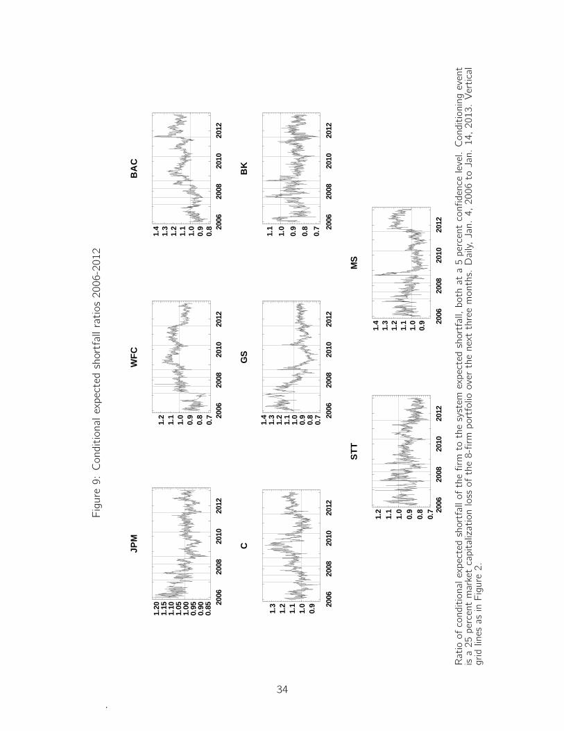
Figure9:Conditionalexpectedshortfallratios2006-2012

2006

2008

2010

2012

0.85

0.90

0.95

1.00

1.05

1.10

1.15

1.20

JPM

2006

2008

2010

2012

0.7

0.8

0.9

1.0

1.1

1.2

WF

C

2006

2008

2010

2012

0.8

0.9

1.0

1.1

1.2

1.3

1.4

BA

C

2006

2008

2010

2012

0.9

1.0

1.1

1.2

1.3

C

2006

2008

2010

2012

0.7

0.8

0.9

1.0

1.1

1.2

1.3

1.4

GS

2006

2008

2010

2012

0.7

0.8

0.9

1.0

1.1

BK

2006

2008

2010

2012

0.7

0.8

0.9

1.0

1.1

1.2

ST

T

2006

2008

2010

2012

0.9

1.0

1.1

1.2

1.3

1.4

MS

Ratioofconditionalexpectedshortfallofthefirmtothesystemexpectedshortfall,bothata5percentconfidencelevel.Conditioningevent

isa25percentmarketcapitalizationlossofthe8-firmportfoliooverthenextthreemonths.Daily,Jan.4,2006toJan.14,2013.Vertical

gridlinesasinFigure2.

34

Figure 10: Expected shortfall elasticities 2006-2012

C

BAC

JPM

WFC

GSMS BK�STT

2006 2008 2010 20120.0

0.2

0.4

0.6

0.8

1.0

The elasticities are displayed cumulatively, so that each plot includes the sharesof all the firms below it. Vertical grid lines as in Figure 2.

35

Figure 11: Conditional expected shortfall and crisis losses

JPMJPM

WFCWFC

BACBAC

CC

GSGS

BKBKSTTSTT

MSMS

0.15 0.16 0.17 0.18 0.19 0.20

0.2

0.4

0.6

0.8

Values on the x-axis are firms’ conditional expected shortfall at the 95 percentlevel (ratio to market capitalization) on July 3, 2008. Values on the y -axis arerealized equity market losses between July 3 and Dec. 31, 2008.

36

Figure 12: Conditional expected shortfall and stress test results

JPMJPMWFCWFC

BACBACCC

GSGS

USBUSB

COFCOF

METMET

MSMS

AXPAXPBKBK

PNCPNC

STTSTT

BBTBBT

STISTI

FITBFITB

RFRFKEYKEY

0.26 0.28 0.30 0.32 0.34 0.36 0.38

�0.2

0.0

0.2

0.4

0.6

Values on the x-axis are the firm’s average conditional expected shortfall atthe 95 percent level (ratio to market capitalization) between Feb. 10 and Mar.8, 2012. Values on the y -axis are −1× the ratio of each firm’s Net Incomebefore Taxes, Table 4 of Board of Governors of the Federal Reserve System(2012), to average market capitalization between Feb. 10 and Mar. 8, 2012.

37

Figure 13: Conditional expected shortfall and V-Lab marginal expected shortfall

JPMJPMWFCWFC

BACBAC

CC

GSGS

USBUSB

COFCOF METMET

MSMS

AXPAXP

BKBK

PNCPNC

STTSTT

BBTBBT

STISTIFITBFITB RFRF

KEYKEY

0.26 0.28 0.30 0.32 0.34 0.36 0.382

3

4

5

6

Values on the x-axis are the firm’s average conditional expected shortfall atthe 95 percent level (ratio to market capitalization), Apr. 2-30, 2012. Valueson the y -axis are MES for Apr. 30, 2012 from http://vlab.stern.nyu.edu/analysis/RISK.USFIN-MR.MES.

38