the impact of smoothness on model class selection in nonlinear system identification
TRANSCRIPT

The Impact of Smoothness on Model ClassSelection in Nonlinear System Identification:
An Application of Derivatives in the RKHS
Y. Bhujwalla, V. Laurain, M. Gilson
6th July [email protected]
Yusuf Bhujwalla (Université de Lorraine) IEEE ACC 2016 1 / 23

Introduction
The Data-Generating SystemMeasured data : DN = {(u1, y1), (u2, y2), . . . , (uN , yN)}.Describes So, an unknown nonlinear system with function fo : X → R,
So :
!
yo,k = fo(xk)yk = yo,k + eo,k
Where xk = [yk−1 · · · yk−na uk · · · uk−nb ]⊤ ∈ X = R
na+nb+1.
Parametric ModelsNθ low (fixed)
↪→ Physically interpretable !
Choice of basis function ?↪→ Combinatorially hard problem X
Nonparametric ModelsNθ high (∼ data)
↪→ Not interpretable XCan define a general model class.
↪→ Flexibility !
Yusuf Bhujwalla (Université de Lorraine) IEEE ACC 2016 2 / 23

Introduction
The Data-Generating SystemMeasured data : DN = {(u1, y1), (u2, y2), . . . , (uN , yN)}.Describes So, an unknown nonlinear system with function fo : X → R,
So :
!
yo,k = fo(xk)yk = yo,k + eo,k
Where xk = [yk−1 · · · yk−na uk · · · uk−nb ]⊤ ∈ X = R
na+nb+1.
Parametric ModelsNθ low (fixed)
↪→ Physically interpretable !
Choice of basis function ?↪→ Combinatorially hard problem X
Nonparametric ModelsSuch as kernel methods :
Input0 0.1 0.2 0.3 0.4 0.5 0.6 0.7 0.8 0.9 1
Out
put
0
0.5
1
1.5
2yokx
Yusuf Bhujwalla (Université de Lorraine) IEEE ACC 2016 2 / 23

Outline
1 Kernel Methods in Nonlinear Identification
2 The Kernel Selection Problem
3 Smoothness in the RKHS
4 Simulation Examples
Yusuf Bhujwalla (Université de Lorraine) IEEE ACC 2016 3 / 23

1. Kernel Methods in Nonlinear IdentificationReproducing Kernel Hilbert Spaces
Hilbert SpacesH is a space over a class of functions, f : X → R ∈ H :
· ∥ f ∥H· ⟨ f , g ⟩H.
In system identification, H ⇔ model class.
Reproducing KernelsH has a unique, associated kernel function, K : X ×X → R, spanning the spaceH.The Reproducing Property states that f (x) can be explicitly represented as aninfinite sum in terms of the kernel function :
f (x) = ⟨ f ,Kx⟩H =∞"
i=1
αiK(xi, x)
Yusuf Bhujwalla (Université de Lorraine) IEEE ACC 2016 4 / 23

1. Kernel Methods in Nonlinear IdentificationIdentification in the RKHS
Identification in the RKHSFor f̂ ∈ H close to fo, f̂ should reflect observations :
f̂ = minf
{ V( f ) = L(x, y, f (x)) }
However, infinitely many solutions ⇒ add constraint to model :
f̂ = minf
{V( f ) = L(x, y, f (x)) + g(∥ f∥H) }
For such cost-functions, f (x) can be reduced to :
f (x) =N"
i=1
αiK(xi, x), α ∈ RN
· f (x) → a finite sum over the observations.· The Representer Theorem (Schölkopf, Herbrich and Smola, 2001)
Yusuf Bhujwalla (Université de Lorraine) IEEE ACC 2016 5 / 23

1. Kernel Methods in Nonlinear IdentificationA Widely-Used Example
A Widely-Used ExampleAs an example minimise squared-error :
L(x, y, f (x)) = ∥y− f (x)∥22,
and use regularisation to avoid overparameterisation :
g(∥ f∥H) = λ∥ f∥2H.
Giving :
Vf : V( f ) = ∥y− f (x)∥22 + λf∥ f∥2H⇒ αf = (K+ λf I)−1 y
· Solution depends onI. K and
II. λf
Yusuf Bhujwalla (Université de Lorraine) IEEE ACC 2016 6 / 23

Outline
1 Kernel Methods in Nonlinear Identification
2 The Kernel Selection Problem
3 Smoothness in the RKHS
4 Simulation Examples
Yusuf Bhujwalla (Université de Lorraine) IEEE ACC 2016 7 / 23

2. The Kernel Selection ProblemChoosing a Kernel Function
Choosing a kernel function...K defines the model classLet X = R, and K be the GaussianRBF kernel :
K(xi, x) = exp!
−∥x− xi∥2
σ2
#
.
Width (σ) defines smoothness ofthe kernel function.Hence σ determines the modelclass !Other kernels have differenthyperparameters, but they will stillinfluence H.
Input-1 -0.5 0 0.5 1
0
0.2
0.4
0.6
0.8
1
Input-1 -0.5 0 0.5 1
0
0.2
0.4
0.6
0.8
1
K xK x
σ1
σ2 > σ1
σ
Yusuf Bhujwalla (Université de Lorraine) IEEE ACC 2016 8 / 23

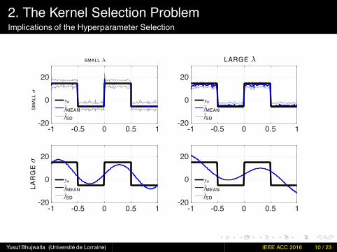
2. The Kernel Selection ProblemImplications of the Hyperparameter Selection
Estimation of 1D switching signalusing Vf = ∥y− f (x)∥22 + λf∥f∥2H.Many observations (N = 103).uk ∼ U(−1, 1).Significant noise disturbances(SNR = 5dB).Two hyperparameters :
I. σ andII. λ
-1 -0.5 0 0.5 1-20
-10
0
10
20
30
f o(u
k)uk
FIGURE: Estimation of 1D switchingsignal for different hyperparametervalues.
Yusuf Bhujwalla (Université de Lorraine) IEEE ACC 2016 9 / 23
2. The Kernel Selection ProblemImplications of the Hyperparameter Selection
-1 -0.5 0 0.5 1-20
0
20
-1 -0.5 0 0.5 1-20
0
20
-1 -0.5 0 0.5 1-20
0
20
-1 -0.5 0 0.5 1-20
0
20
yoyo
yoyo
f̂MEANf̂MEAN
f̂MEANf̂MEAN
f̂SDf̂SD
f̂SDf̂SD
SMALL λ LARGE λ
SM
ALL
σLA
RG
Eσ
Yusuf Bhujwalla (Université de Lorraine) IEEE ACC 2016 10 / 23
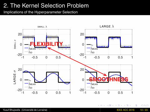
2. The Kernel Selection ProblemImplications of the Hyperparameter Selection
-1 -0.5 0 0.5 1-20
0
20
-1 -0.5 0 0.5 1-20
0
20
-1 -0.5 0 0.5 1-20
0
20
-1 -0.5 0 0.5 1-20
0
20
SMOOTHNESS
FLEXIBILITY
yoyo
yoyo
f̂MEANf̂MEAN
f̂MEANf̂MEAN
f̂SDf̂SD
f̂SDf̂SD
SMALL λ LARGE λ
SM
ALL
σLA
RG
Eσ
Yusuf Bhujwalla (Université de Lorraine) IEEE ACC 2016 10 / 23

2. The Kernel Selection ProblemSummary
SummaryVf : V(f ) = ∥y− f (x)∥22 + λf∥ f∥2H.
Kernel framework very effective :· flexible,· well-understood.
However, choice of kernel often compromised (e.g. by noise).⇒ Trade-off between flexibility and smoothness.
So, why regularise over ∥ f∥H . . .. . . when smoothness is often a more interesting property to control ?⇒ Desirable property in many models.⇒ Characterises many systems.
Yusuf Bhujwalla (Université de Lorraine) IEEE ACC 2016 11 / 23

Outline
1 Kernel Methods in Nonlinear Identification
2 The Kernel Selection Problem
3 Smoothness in the RKHS
4 Simulation Examples
Yusuf Bhujwalla (Université de Lorraine) IEEE ACC 2016 12 / 23
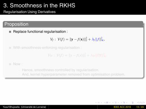
3. Smoothness in the RKHSRegularisation Using Derivatives
PropositionReplace functional regularisation :
Vf : V(f ) = ∥y− f (x)∥22 + λf∥ f∥2H,
With smoothness-enforcing regularisation :
VD : V(f ) = ∥y− f (x)∥22 + λD∥Df∥2H.
Now :· Hence, smoothness controlled by regularisation.· And, kernel hyperparameter removed from optimisation problem.
Yusuf Bhujwalla (Université de Lorraine) IEEE ACC 2016 13 / 23
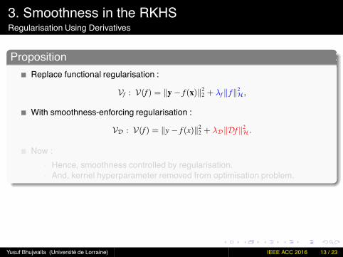

3. Smoothness in the RKHSDerivatives in the RKHS
Derivatives in the RKHSFor f ∈ H, Df ∈ H (Zhou, 2008)Hence, a derivative reproducing property can be defined :
Df = ⟨ f ,DKx ⟩H
The Representer TheoremRepresenter f (x) =
$Ni=1 αiK(xi, x) requires
g(∥ f∥H) : a monotically increasing function of ∥ f∥H
Clearly, ∥Df∥H ! g(∥ f∥H) ⇒ representer is suboptimal for VD.However, if system is well-excited, f (x) =
$Ni=1 αiK(xi, x) can be used.
However, it loosely preserves the bias-variance properties of Vf
limλ→∞
f (x) = 0, ∀x ∈ R.
Yusuf Bhujwalla (Université de Lorraine) IEEE ACC 2016 14 / 23

3. Smoothness in the RKHSDerivatives in the RKHS
A Closed-Form SolutionUsing derivative reproducing property, ∥Df∥H can be defined :
∥Df∥2H = α⊤D(1, 1)Kα,
whereD(1, 1)K(xi, xj) =
∂2K(xi, xj)∂xj ∂xi
.
Permitting a closed-form solution :
αD =%
K⊤K+ λDD(1, 1)K&−1
K⊤y.
As per Vf ⇒ αf = (K+ λf I)−1 y.
Yusuf Bhujwalla (Université de Lorraine) IEEE ACC 2016 15 / 23

Outline
1 Kernel Methods in Nonlinear Identification
2 The Kernel Selection Problem
3 Smoothness in the RKHS
4 Simulation Examples
Yusuf Bhujwalla (Université de Lorraine) IEEE ACC 2016 16 / 23

4. Simulation ExamplesExample 1 : Effect of the Regularisation
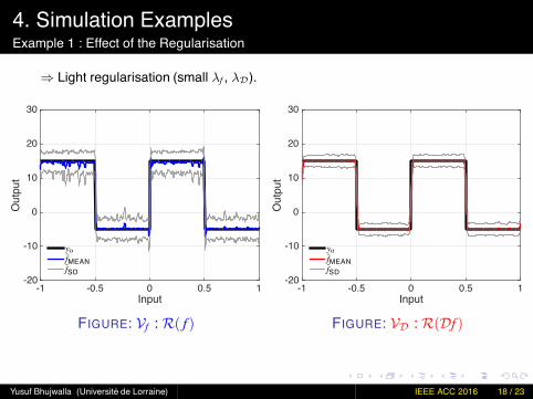
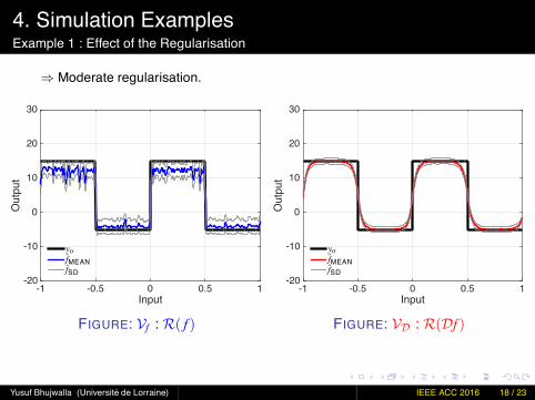
Estimation of 1D switching signalusing Vf and VD.Many observations (N = 103).uk ∼ U(−1, 1).Significant noise disturbances(SNR = 5dB).Gaussian RBF kernel, with σ = 0.01.Varying levels of regularisation(through λf , λD).
-1 -0.5 0 0.5 1-20
-10
0
10
20
30
f o(u
k)uk
FIGURE: Estimation of 1D switchingsignal for different λ values.
Yusuf Bhujwalla (Université de Lorraine) IEEE ACC 2016 17 / 23

4. Simulation ExamplesExample 1 : Effect of the Regularisation
⇒ Negligible regularisation (very small λf , λD).
Input-1 -0.5 0 0.5 1
Out
put
-20
-10
0
10
20
30
yof̂MEANf̂SD
FIGURE: Vf : R( f )
Input-1 -0.5 0 0.5 1
Out
put
-20
-10
0
10
20
30
yof̂MEANf̂SD
FIGURE: VD : R(Df )
Yusuf Bhujwalla (Université de Lorraine) IEEE ACC 2016 18 / 23
4. Simulation ExamplesExample 1 : Effect of the Regularisation
⇒ Light regularisation (small λf , λD).
Input-1 -0.5 0 0.5 1
Out
put
-20
-10
0
10
20
30
yof̂MEANf̂SD
FIGURE: Vf : R( f )
Input-1 -0.5 0 0.5 1
Out
put
-20
-10
0
10
20
30
yof̂MEANf̂SD
FIGURE: VD : R(Df )
Yusuf Bhujwalla (Université de Lorraine) IEEE ACC 2016 18 / 23
4. Simulation ExamplesExample 1 : Effect of the Regularisation
⇒ Moderate regularisation.
Input-1 -0.5 0 0.5 1
Out
put
-20
-10
0
10
20
30
yof̂MEANf̂SD
FIGURE: Vf : R( f )
Input-1 -0.5 0 0.5 1
Out
put
-20
-10
0
10
20
30
yof̂MEANf̂SD
FIGURE: VD : R(Df )
Yusuf Bhujwalla (Université de Lorraine) IEEE ACC 2016 18 / 23

4. Simulation ExamplesExample 1 : Effect of the Regularisation
⇒ Heavy regularisation (large λf , λD).
Input-1 -0.5 0 0.5 1
Out
put
-20
-10
0
10
20
30
yof̂MEANf̂SD
FIGURE: Vf : R( f )
Input-1 -0.5 0 0.5 1
Out
put
-20
-10
0
10
20
30
yof̂MEANf̂SD
FIGURE: VD : R(Df )
Yusuf Bhujwalla (Université de Lorraine) IEEE ACC 2016 18 / 23

4. Simulation ExamplesExample 1 : Effect of the Regularisation
⇒ Excessive regularisation (very large λf , λD).
Input-1 -0.5 0 0.5 1
Out
put
-20
-10
0
10
20
30
yof̂MEANf̂SD
FIGURE: Vf : R( f )
Input-1 -0.5 0 0.5 1
Out
put
-20
-10
0
10
20
30
yof̂MEANf̂SD
FIGURE: VD : R(Df )
Yusuf Bhujwalla (Université de Lorraine) IEEE ACC 2016 18 / 23

4. Simulation ExamplesExample 2 : 1D Structural Selection
Identification of two unknown systems (X ∈ [−1, 1], SNR = 10dB, N = 103).Vf : λ, σ optimised using cross-validation.VD : λ optimised using cross-validation, σ set based on data.
-0.5 0 0.5-10
-5
0
5
10
15
20
25
f1 o(u
k)
ukFIGURE: S1o : Smooth
-0.5 0 0.5-10
-5
0
5
10
15
20
25
f2 o(u
k)
ukFIGURE: S2o : Nonsmooth
Yusuf Bhujwalla (Université de Lorraine) IEEE ACC 2016 19 / 23

4. Simulation ExamplesExample 2 : Smooth S1o
Using a small kernel, VD can reconstruct a smooth function.Not feasible using Vf - needs kernel smoothing effect.
Input-0.5 0 0.5
Out
put
-10
-5
0
5
10
15
20
25f̂MEAN
f̂SD
kx
FIGURE: Vf : R( f )
Input-0.5 0 0.5
Out
put
-10
-5
0
5
10
15
20
25f̂MEAN
f̂SD
kx
FIGURE: VD : R(Df )
Yusuf Bhujwalla (Université de Lorraine) IEEE ACC 2016 20 / 23

4. Simulation ExamplesExample 2 : Nonsmooth S2o
Using a small kernel, VD can detect structural nonlinearity.However, Vf is too smooth, as σ must counteract noise.
Input-0.5 0 0.5
Out
put
-10
-5
0
5
10
15
20
25f̂MEAN
f̂SD
kx
FIGURE: Vf : R( f )
Input-0.5 0 0.5
Out
put
-10
-5
0
5
10
15
20
25f̂MEAN
f̂SD
kx
FIGURE: VD : R(Df )
Yusuf Bhujwalla (Université de Lorraine) IEEE ACC 2016 21 / 23

Conclusions
RKHS in Nonlinear IdentificationFlexible framework : attractive for nonlinear identification.Smoothness controlled by kernel function and regularisation (σ and λf )⇒ Constrained kernel function.
Derivatives in the RKHSSmoothness controlled by regularisation (λD).⇒ Simpler steering of the smoothness.Simpler hyperparameter optimisation (just λD) and increased model flexibility.⇒ Through use of a smaller kernel (small σ).However, relies on a suboptimal representer.⇒ Nonetheless, promising results have been obtained.
Yusuf Bhujwalla (Université de Lorraine) IEEE ACC 2016 22 / 23

The Impact of Smoothness on Model ClassSelection in Nonlinear System Identification:
An Application of Derivatives in the RKHS
Y. Bhujwalla, V. Laurain, M. Gilson
6th July [email protected]
Yusuf Bhujwalla (Université de Lorraine) IEEE ACC 2016 23 / 23

A. BibliographyAlternative Smoothness-Enforcing Optimisation Schemes
Sobolev Spaces (Wahba, 1990 ; Pillonetto et al, 2014)
∥f∥Hk
=m
"
i=0
'
X
(
dif (x)dxi
)2
dx
Identification using derivative observations (Zhou, 2008 ; Rosasco et al, 2010)
Vobvs( f ) = ∥y− f (x)∥22 + γ1
*
*
*
*
dydx
−df (x)dx
*
*
*
*
2
2
+ · · · γm
*
*
*
*
dmydxm
−dmf (x)dxm
*
*
*
*
2
2+ λ ∥f∥
H
Regularization Using Derivatives (Rosasco et al, 2010 ; Lauer, Le and Bloch,2012 ; Duijkers et al, 2014)
VD( f ) = ∥y− f (x)∥22 + λ∥Dmf∥p.
Yusuf Bhujwalla (Université de Lorraine) IEEE ACC 2016 23 / 23

A. BibliographyLiterature Review
Kernel Methods in Machine Learning and System Identification· Kernel methods in system identification, machine learning and functionestimation : A survey, G. Pillonetto, F. Dinuzzo, T. Chen, G. D. Nicolao and L.Ljung, 2014.
· Learning with Kernels, B. Schölkopf, R. Herbrich and A. J. Smola, 2002.· Gaussian Processes for Machine Learning, C. Rasmussen and C. Williams,
2006.
Reproducing Kernel Hilbert Spaces· Theory of Reproducing Kernels, N. Aronszajn, 1950.· A Generalized Representer Theorem, B. Schölkopf, R. Herbrich and A. J. Smola,
2001.· Derivative reproducing properties for kernel methods in learning theory, D. Zhou,
2008.
Yusuf Bhujwalla (Université de Lorraine) IEEE ACC 2016 23 / 23

B. Example 2 : 1D Structural SelectionS1o : Smooth
Input-0.5 0 0.5
Out
put
-10
-5
0
5
10
15
20
25f̂MEAN
f̂SD
kx
FIGURE: Vf : R( f )
Input-0.5 0 0.5
Out
put
-10
-5
0
5
10
15
20
25f̂MEAN
f̂SD
kx
FIGURE: VD : R(Df )
Yusuf Bhujwalla (Université de Lorraine) IEEE ACC 2016 23 / 23

B. Example 2 : 1D Structural SelectionS2o : Nonsmooth
Input-0.5 0 0.5
Out
put
-10
-5
0
5
10
15
20
25f̂MEAN
f̂SD
kx
FIGURE: Vf : R( f )
Input-0.5 0 0.5
Out
put
-10
-5
0
5
10
15
20
25f̂MEAN
f̂SD
kx
FIGURE: VD : R(Df )
Yusuf Bhujwalla (Université de Lorraine) IEEE ACC 2016 23 / 23
C. Applicability of the RepresenterKernel Density
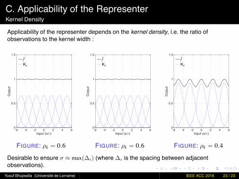
Applicability of the representer depends on the kernel density, i.e. the ratio ofobservations to the kernel width :
Input (x/σ)-6 -4 -2 0 2 4 6
Out
put
0
0.5
1
1.5f̂Kx
FIGURE: ρk = 0.6
Input (x/σ)-6 -4 -2 0 2 4 6
Out
put
0
0.5
1
1.5f̂Kx
FIGURE: ρk = 0.6
Input (x/σ)-6 -4 -2 0 2 4 6
Out
put
0
0.5
1
1.5f̂Kx
FIGURE: ρk = 0.4
Desirable to ensure σ ≈ max(∆x) (where ∆x is the spacing between adjacentobservations).
Yusuf Bhujwalla (Université de Lorraine) IEEE ACC 2016 23 / 23