Nonlinear System Identification and Modeling of A New FatigueTesting Rig Based on Inertial Forces

Michael Falco, Ming Liu, Son Hai Nguyen and David Chelidze∗Department of Mechanical, Industrial and Systems Engineering

University of Rhode Island, Kingston, RI 02881Email: chelidze@egr.uri.edu

A novel fatigue testing rig based on inertial forces is in-troduced. The test rig has capacity to mimic various loadingconditions including high frequency loads. The rig design al-lows reconfigurations to accommodate a range of specimensizes, and changes in structural elements and instrumenta-tion. It is designed to be used as a platform to study the in-teraction between fatigue crack propagation and structuraldynamics. As the first step to understand this interaction, anumerical model of testing rig is constructed using nonlinearsystem identification approaches. Some initial testing resultsalso are reported.

1 IntroductionMaterial fatigue has been a subject of great interest since

the 1840’s. Pioneered by Wilhelm Albert [1], scientists andengineers use fatigue testing rigs as powerful tools to validatetheories and mechanical designs, and fatigue tests have be-come a critical procedure for manufacturing industry [2, 3].To be competitive in the modern market, additional require-ments are posed: fatigue tests have to be conducted quicklyand be able to fit into fast product development cycles; andthe tests have to reflect real load scenarios, so over-designcan be avoided without damaging reliability.

Traditional fatigue testing rigs have difficulty to meetboth of the requirements at the same time. Based on meth-ods of load application, the testing rigs can be classifiedinto [4, 5]: 1) spring, 2) centrifugal, 3) hydraulic, 4) pneu-matic, 5) thermal dilatation, and 6) electro-magnetic forcebased loads. Among these rigs, 1), 2), and 6) usually canonly provide periodic loads; and 3), 4), and 5) are limited bytheir low frequency load application. Although literature re-views also show fatigue testing machines with ultrahigh ex-citation frequency [6], these rigs are designed for tiny com-ponents which are beyond the range of discussion here.

A novel fatigue testing rig based on inertial forces is de-

∗Address all correspondence to this author.

signed and constructed at the University of Rhode Island’sNonlinear Dynamics Laboratory. This new rig can dupli-cate arbitrary load histories with a high testing frequency (30Hz or above), at the same time, it permitts fatigue tests atvarious R-ratios1 (including zero or negative), which can becontrolled accurately and is adjustable during a test. Thiswork was motivated by similar testing rig [7]. However, ourhorizontal—in contrast with their vertical— arrangement al-lows for more range in loading rates and frequencies, and fa-cilitates reconfigurable test design. Our system can be easilyreconfigured to accommodate range of different specimens,as well as changes to other structural elements and sensinginstrumentation.

In a mechanical structure, fatigue crack propagation isnot an isolated process. Fatigue process is driven by thestructural dynamics, but fatigue also affects this dynamics bychanging structural parameters. Hence, fatigue life predic-tion methods cannot be accurate without taking into consid-eration this interaction between crack propagation and struc-tural dynamics. However, traditional life prediction modelsusually ignore structural dynamics when estimating stresses.In particular, based on our preliminary testing, we have re-ported in Ref. [8] that the Palmgren-Miner rule and rain-flowcounting method, which are the most widely used in indus-try, fail for stationary chaotic loading by consistently overes-timating fatigue damage. Therefore, there is a need to inves-tigate the effect of the structural dynamics on fatigue crackgrowth and damage accumulation.

Equipped with multiple sensors and a high performanceDAQ system, the fatigue testing rig can serve as a perfectplatform to study the interaction between fatigue crack prop-agation and structural dynamics. As the first step of relatedresearch, a reliable model of the healthy structure (the rigwithout cracks) is constructed. This model not only de-scribes the dynamics of the structure, but serves as a baseline

1R = σmin/σmax, where σmin is the minimum peak stress and σmax is themaximum peak stress

Fig. 1: Schematic of the fatigue testing apparatus. 1. Flexibleconnector; 2. Slip table; 3. Back cylinder; 4. Rail; 5. Backmass block; 6. Specimen supports; 7. Specimen; 8. Frontmass block; 9. Front cylinder.

for future modeling efforts. Due to the inherent nonlinear-ity of the rig, a linear model is inadequate to describe fulldynamical properties of the structure accurately. A nonlin-ear model is constructed using restoring force surface (RFS)and direct parameter estimation (DPE) methodology. A lin-ear model is also generated for validation purpose based onmodal analysis results.

To validate usefulness of this new setup, several initialtests have been conducted. The collected data are used tocompare the Generalized Fatigue Damage Coordinate’s, cal-culated based on Phase Space Warping [9–11] and SmoothOrthogonal Decomposition [12], with direct fatigue crackmeasurements from and Alternating Current Potential Drop(ACPD) crack monitoring system.

In the next section the setup of the fatigue testing rig isdescribed. Following it with some initial testing results, thedetails of the nonlinear system identification, and additionaldiscussion about the inherent nonlinearity.

2 Fatigue Testing Rig2.1 Mechanical Setup

A schematic of the testing rig is shown in Fig. 1. Themechanical backbone of the system is a slip table guided byfour linear bearings on two parallel rails mounted to a gran-ite base. An LDS electromagnetic shaker (V721 Bruel &Kjær, German), whose maximum frequency is about 4kHz,is used to drive the slip table and mimic various loading con-ditions. The specimen is a single-edge notched beam, whichis pin-pin supported. Two inertial mass blocks, guided bylinear bearings mounted to the slip table, provide dynamicloads. The masses are kept in contact with the specimen bytwo pneumatic cylinders. When the slip table moves, themasses transfer inertial forces to the specimen. The appliedloads on the specimen are shown in Fig. 2, where m1 andm2 are the masses of the back and front mass, respectively;

P1 +m1arel

P2 −m2arel2

P2 −m2arel2

arel

arelm1

m2

Fig. 2: Beam diagram with applied forces

Fig. 3: Photograph of the system

P1 and P2 are the forces due to the pressures within the backand front cylinders; and arel is the relative acceleration be-tween the masses and the slip table. In order to keep themass blocks in contact with the specimen at all times, pres-sures within the cylinders are set so that P1 > m1 min(arel)and P2 > m2 max(arel). Different R-ratios can be obtainedby adjusting the pressure in each cylinder and the amplitudeof the signal supplied to the shaker. A photo of the system isincluded in Fig. 3.

The specimens are designed to follow the ASTM stan-dard E1820-08a [13], and their drawing is shown in Fig. 4.They are made of 6061 aluminum bar stock, with dimensions314.70× 20.32× 6.35 mm (length × height × width), andthe fatigue is initiated by a machined ‘V’ notch. The notchis cut to a depth of 7.62 mm by a blade 0.762 mm thick witha 60 ◦ V-shaped tip. In order to get rid of residual and ma-chining stresses, the specimens are fully annealed prior totesting.

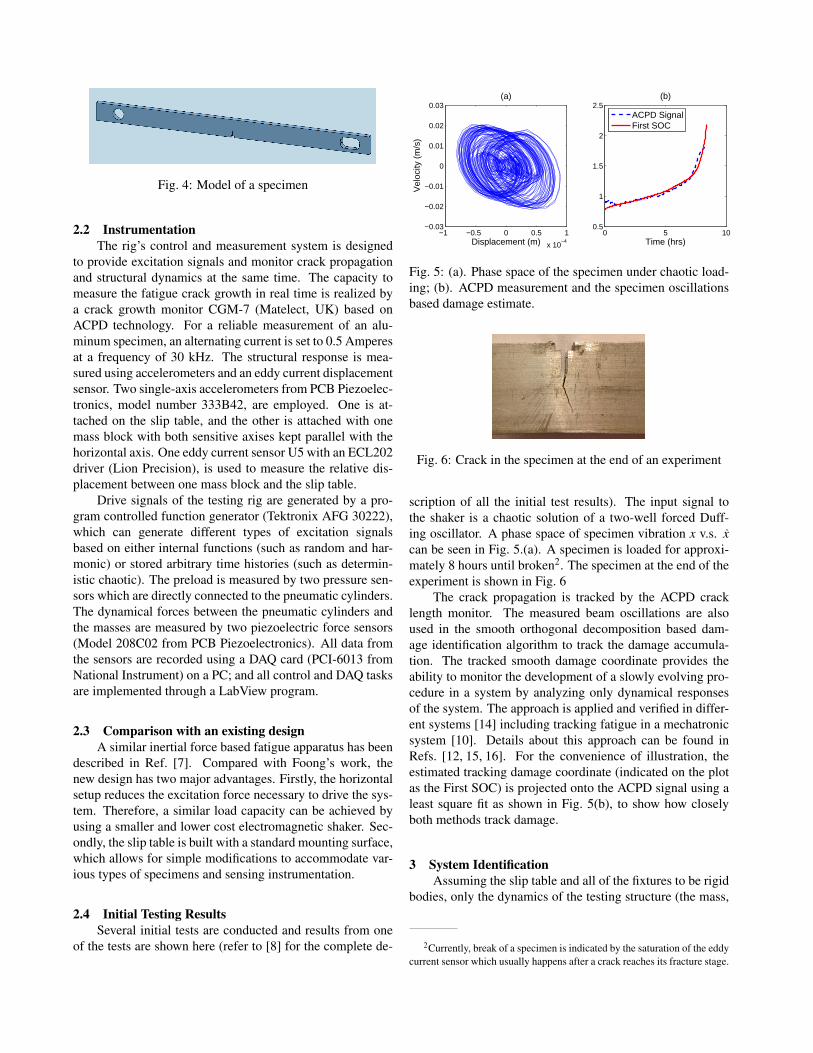
Fig. 4: Model of a specimen

2.2 InstrumentationThe rig’s control and measurement system is designed

to provide excitation signals and monitor crack propagationand structural dynamics at the same time. The capacity tomeasure the fatigue crack growth in real time is realized bya crack growth monitor CGM-7 (Matelect, UK) based onACPD technology. For a reliable measurement of an alu-minum specimen, an alternating current is set to 0.5 Amperesat a frequency of 30 kHz. The structural response is mea-sured using accelerometers and an eddy current displacementsensor. Two single-axis accelerometers from PCB Piezoelec-tronics, model number 333B42, are employed. One is at-tached on the slip table, and the other is attached with onemass block with both sensitive axises kept parallel with thehorizontal axis. One eddy current sensor U5 with an ECL202driver (Lion Precision), is used to measure the relative dis-placement between one mass block and the slip table.

Drive signals of the testing rig are generated by a pro-gram controlled function generator (Tektronix AFG 30222),which can generate different types of excitation signalsbased on either internal functions (such as random and har-monic) or stored arbitrary time histories (such as determin-istic chaotic). The preload is measured by two pressure sen-sors which are directly connected to the pneumatic cylinders.The dynamical forces between the pneumatic cylinders andthe masses are measured by two piezoelectric force sensors(Model 208C02 from PCB Piezoelectronics). All data fromthe sensors are recorded using a DAQ card (PCI-6013 fromNational Instrument) on a PC; and all control and DAQ tasksare implemented through a LabView program.

2.3 Comparison with an existing designA similar inertial force based fatigue apparatus has been

described in Ref. [7]. Compared with Foong’s work, thenew design has two major advantages. Firstly, the horizontalsetup reduces the excitation force necessary to drive the sys-tem. Therefore, a similar load capacity can be achieved byusing a smaller and lower cost electromagnetic shaker. Sec-ondly, the slip table is built with a standard mounting surface,which allows for simple modifications to accommodate var-ious types of specimens and sensing instrumentation.

2.4 Initial Testing ResultsSeveral initial tests are conducted and results from one

of the tests are shown here (refer to [8] for the complete de-

−1 −0.5 0 0.5 1

x 10−4

−0.03

−0.02

−0.01

0

0.01

0.02

0.03

Displacement (m)

Vel

ocity

(m

/s)

(a)

0 5 100.5

1

1.5

2

2.5

Time (hrs)

(b)

ACPD SignalFirst SOC

Fig. 5: (a). Phase space of the specimen under chaotic load-ing; (b). ACPD measurement and the specimen oscillationsbased damage estimate.

Fig. 6: Crack in the specimen at the end of an experiment

scription of all the initial test results). The input signal tothe shaker is a chaotic solution of a two-well forced Duff-ing oscillator. A phase space of specimen vibration x v.s. xcan be seen in Fig. 5.(a). A specimen is loaded for approxi-mately 8 hours until broken2. The specimen at the end of theexperiment is shown in Fig. 6

The crack propagation is tracked by the ACPD cracklength monitor. The measured beam oscillations are alsoused in the smooth orthogonal decomposition based dam-age identification algorithm to track the damage accumula-tion. The tracked smooth damage coordinate provides theability to monitor the development of a slowly evolving pro-cedure in a system by analyzing only dynamical responsesof the system. The approach is applied and verified in differ-ent systems [14] including tracking fatigue in a mechatronicsystem [10]. Details about this approach can be found inRefs. [12, 15, 16]. For the convenience of illustration, theestimated tracking damage coordinate (indicated on the plotas the First SOC) is projected onto the ACPD signal using aleast square fit as shown in Fig. 5(b), to show how closelyboth methods track damage.

3 System IdentificationAssuming the slip table and all of the fixtures to be rigid

bodies, only the dynamics of the testing structure (the mass,

2Currently, break of a specimen is indicated by the saturation of the eddycurrent sensor which usually happens after a crack reaches its fracture stage.

specimen, and pneumatic cylinders) are included in the phys-ical model of the testing rig. Because of the nonlinear com-ponents (e.g, pneumatic cylinders), standard modal analy-sis [17] cannot be applied directly. Here, a nonlinear systemidentification procedure is utilized.

Although there is no uniform standard solution for non-linear SID [18], the system identification task is realizedthrough a three step process consisting of nonlinearity de-tection, selection of an appropriate nonlinear model, and es-timation of model parameters. Each step is achieved usingfrequency response function overlay (FRFO), restoring forcesurface (RFS), and direct parameter estimation (DPE) meth-ods, respectively.

3.1 Detection of NonlinearityThe concept of FRFO is that the frequency response

function (FRF) of a linear system is independent of excitationamplitude, which is not true for a nonlinear system. There-fore, nonlinearity can be detected by changes in the FRF as-sociated with the changes in the excitation amplitude [19].Reviews of other nonlinearity detection approaches can befound in Ref. [20].

Standard modal analysis is conducted using an ACEdata acquisition card and Signal Calc modal analysis soft-ware from Data Physics, Inc.. The FRF is calculated fromdata averaged over 16 windows of burst-random excitation.This excitation is chosen to mitigate spectral leakage. Eightypercent of the window size is used for random excitation,while the remaining twenty percent is zero-level excitation.In the experiment, the input signal is from an accelerometermounted to a rigid support, while the output signal is from anaccelerometer mounted to the front mass block. Both signalsare high pass filtered at 5Hz in order to remove low frequencyuncertainties related to accelerometers. Three tests are con-ducted at amplitude levels small, medium and large. Thecorresponding FRF’s are shown in Fig. 7. As the amplitudeincreases, the peaks of the FRF moves towards the lower fre-quency range, which is indicative of a softening spring non-linear characteristic. The FRFs also indicate that the test rigmainly operates in the beam’s first mode of oscillation by nothaving any significant dynamical content at higher frequen-cies (except slip table’s natural frequency at 150 Hz), whichwould have been excited if the masses lost contact with thespecimen.

3.2 Nonlinear Model SelectionThe major challenge in nonlinear system identification is

model selection [18]. Because our testing rig is a relativelysimple system, a two step procedure is adopted to determineappropriate system model. The first step is to build a simplephysical model with some unknown functions. Then the RFSapproach is used to determine the unknown functions andparameters.

0 20 40 60 80 100 120−10

−5

0

5

10

Frequency (Hz)

Mag

nitu

de (

dB)

Small AmplitudeMedium AmplitudeLarge Amplitude

Fig. 7: Frequency response function for different load levels

k1 c1

mx( t)

ks

aBase

k2 c2

Fig. 8: A simplified model for the fatigue testing rig

The assumptions that the slip table and fixtures are rigidand the deformation of the specimen is relatively small (<2×10−4 m from its equilibrium position), and the masses arealways in contact with the specimen, allows the testing rig tobe represented by a single degree-of-freedom mass-spring-damper system shown in Fig. 8. The specimen is modeled asa linear spring (with stiffness ks). The pneumatic cylindersare represented by a combination of nonlinear springs (k1and k2) and nonlinear dampers (c1 and c2). The system canbe described by the differential equation in the form of:

mx+ c1(x, x)+ c2(x, x)+ k1(x, x)

+ k2(x, x)+ ksx =−ma,(1)

where m is the total mass of the two mass blocks; a is the baseacceleration; x is the relative displacement measured by theeddy current sensor, and dots represent time differentiation.Further simplification can be made resulting in:

mx+C(x, x)+K(x, x) =−ma, (2)

where C(x, x) = c1(x, x) + c2(x, x) and K(x, x) = k1(x, x) +k2(x, x)+ ksx.

Fig. 9: Left: Distribution of data points and area used togenerate RFS; Right: Generated RFS.

Restoring force [21] is defined as a variable force thatgives rise to an equilibrium in a physical system. For a SDOFsystem, it can be written as:

f (x, x) = F−mx, (3)

where F is the external force and m is the mass. In our case,the restoring force equals:

f (x, x) =−ma−mx =C(x, x)+K(x, x) . (4)

The related RFS approach is one of the most establishednonlinear system identification methods. Although the RFSmethod is not applied directly in this research, the RFS isconstructed and used to provide valuable information formodel selection. Among all the parameters, the mass is mea-sured directly, a is measured by an accelerometer, x is mea-sured by the eddy current sensor, and x and x are calculatedusing finite difference method. Therefore, the RFS can bedirectly generated based on the collected data sets.

The restoring forces are calculated using 6× 105 datapoints, while the testing rig is driven by a random signalwith limited frequency band (0 to 60Hz). The amplitudeof the excitation is chosen to ensure the availability of pa-rameter identification data within the range of proposed ex-perimental excitation amplitudes. The pressure in the twopneumatic cylinders are set to 0.1034 MPa (15 psi). The dataare recorded with DAQ frequency 1 Khz and the distributionof sample points on the phase plane are shown on Fig. 9.Isolated points related with discrete measurements are in-terpolated into a continuous surface using Sibson’s naturalneighbor method [22], and the measured RFS is shown inFig. 9.

In this paper, we assume that the damping force C(x, x)is a function of x only, and K(x, x) is a function of x only.Therefore, the restoring force f (x, x) = C(x) + K(x). Theforms of C(x) and K(x) are unknown. However, they can beidentified by observing the two slice views of the RFS f (x, x)

−1 0 1

x 10−4

−150

−100

−50

0

50

100

150

Displacement (m)

Res

torin

g F

orce

(N

)

−0.01 0 0.01−40

−30

−20

−10

0

10

20

30

Velocity (m/s)

Res

torin

g F

orce

(N

)

Fig. 10: Left: Slice view of RFS when x = 0; Right: Sliceview of RFS when x = 0.

shown in Fig. 10 with x = 0 and x = 0, respectively. FromFig. 10, it is obviously that K(x) can be described partiallyby cubic polynomial. For C(x), the change in the slope closeto x = 0 indicates that Coulomb damping is also present inthe system.

A good experimental fit of measured damping force dueto Coulomb damping [23] can be described as:

F =C|x|δv sgn x, (5)

where F is the damping force and δv depends on geometry.Therefore, Eq. (2) was rewritten in the form:

mx+C f 1x+C f 2x3 +C f 3|x|α sgn x

+K f 1x+K f 2x3 +K f 3|x|β sgnx =−ma,(6)

where C(x) = C f 1x + C f 2x3 + C f 3|x|α sgn x and K(x) =

K f 1x+K f 2x3 +K f 3|x|β sgnx.

3.3 Parameter EstimationWith an assumed nonlinear model, the SID problem is

solved as a parameter estimation problem. The method ofDPE [24] is applied in this research. To perform DPE, Eq.(6) is rewritten for n discrete measurements in the followingform:

x1 x3

1 |x1|α sgn(x1) x1 x31 |x1|β sgn(x1)

x2 x32 |x2|α sgn(x2) x2 x3

2 |x2|β sgn(x2)...

......

......

...xn x3

n |xn|α sgn(xn) xn x3n |xn|β sgn(xn)

C f 1C f 2C f 3K f 1K f 2K f 3

=

x1 a1x2 a2...

...xn an

[−m−m

](7)

−0.01

0

0.01

−1

0

1

x 10−4

−150

−100

−50

0

50

100

150

Velocity (m/s)Displacement (m)

Res

torin

g F

orce

(N

)

Velocity (m/s)

Dis

plac

emen

t (m

)

−0.01 0 0.01

−1

0

1

x 10−4

2N

4N

6N

8N

10N

12N

14N

16N

Fig. 11: Left: Surface generated using parameters from DPE;Right: The error between the modeled surface and the gen-erated RFS.

When n > 6 and parameters α and β are known, Eq. (7)is an over defined problem which can be solved by using astandard least squares approach. To determine the optimal α

and β constants, the procedure introduced in [25] is adopted.A search for optimal α & β begins with a given step size(called grid) in a region around a pre-defined initial point(called the center) [α0, β0]. Then the center is moved tothe point [α1, β1] on the grid, where the least square erroris minimized based on the over-defined Eq. (7). The searchprocedure is repeated with a half grid size. These proceduresare repeated m times until the value |[αm−1,βm−1]− [αm,βm]|is smaller than a specified threshold.

The parameters are determined using the data shown inFig. 9. Then an RFS is generated based on the selected non-linear model and estimated parameters. The resulting surfaceand the error between the modeled surface and the RFS areshown in Fig. 11. The largest absolute value of error is onlyabout 16 N only near the extreme displacements.

4 Discussion4.1 Error Factors

Although the two RFS’s (based on the measured dataand the model) fit each other quite well, relatively large er-rors are observed in the areas when the absolute value of xand x are large and xx > 0. The errors are due to the follow-ing factors:

1. The number of sampling points in these areas is small,which leads to inaccurate estimation of the RFS fromexperimental data.

2. These areas represent rare dynamical states of therig—large displacement, velocity, acceleration, and jerk(large |...x | value), which make the numerical calculationof velocity and acceleration inaccurate.

3. With a large jerk, a time delay between different mea-surement channels on the DAQ system is not ignorable

and causes additional errors in the calculation of accel-eration.

4.2 Dynamic RangeThere are three factors which determine the dynamic

range of the rig: the maximum output force of the shakerFmax = 3700 N, the allowable movement range of the shakerD = 0.0254 m (peack-to-peack), and the natural frequencyof the slip table fN = 150 Hz. Because the total mass of themoving parts (the slip table and the armature moving mass)mtotal is about 45 kg, the maximum acceleration of the slip ta-ble can be determined by amax = Fmax/mtotal = 82.2 m/s2 orabout 8.4 g. Unfortunately, the AC current in the lab is lim-ited to 15 A (while 25 A is needed for full capacity). Thus,the maximum acceleration could only reach 3 g in a shorttime period. For safety reasons, the maximum accelerationis limited to 2 g in actual experiments.

If we assume the excitation signals are sinusoidal, the re-lationship between amax, D, and the excitation frequency fecan be written as: amax = 4π2 f 2

e D/2. Since D = 0.0254 mand amax < 2 g, the maximum acceleration could only bereached only when fe > 6.3 Hz. Because of the natural fre-quency of the slip table is 150 Hz, it is reasonable to limitthe excitation frequency below 30 Hz. Hence the maximumacceleration output of the slip table can only be reached be-tween 6.3 Hz and 30 Hz.

Although increasing the mass of the blocks can improvethe maximum dynamic load on the specimen, this load mustbe smaller than the output of the pneumatic cylinders to keepthe mass blocks in continuous contact with the specimen.At the same time, increase in the mass will cause additionalfriction on the rails. Considering that the mass blocks con-tain about 20% of the mtotal already, the potential to increasethe load capacity by increasing the mass of the blocks is re-stricted. Further improvement of the structural stiffness isalso not pursued, because increasing stiffness leads to addi-tional mass for the slip table, therefore the maximum loadcapacity is limited by the maximum shaker output force.

4.3 Influence of Air PressureThe same system identification procedure is repeated

several times under different pressures (the pressure in thetwo cylinders are kept identical). The estimated parametersare listed in Table 1. The comparison between the measuredbase acceleration and the simulated response based on Eq.(6) is shown in Fig. 12. The stiffness and the damping ofthe testing system increase with the increase of pressure. Weshould note that the coefficient C f 2 had no considerable ef-fect on the quality of the fit and was set to zero. Also, thelinear damping coefficient C f 1 for the lowest load level hasno major effect on the fit, and the negative linear dampingcoefficients for higher loads do not indicate negative damp-ing at low aptitudes, but are actually asymptotic corrections

0 50 100 150 200 250 300 350 400 450 500−20

−15

−10

−5

0

5

10

15

20

time (ms)

a (m

/s2 )

Fig. 12: Comparison between the measured base accelera-tion (thin red line) and the simulated base acceleration (thickblue line) for 0.1034 MPa in the cylinders

to the slope of damping curves at large values of velocity.

4.4 Linear RegionAlthough the testing rig is characterized as having cubic

stiffness, the nonlinearity is not strong especially when theresponse amplitude is relatively small. Therefore it is possi-ble to define a small linear region in which the system canbe treated linear. The definition of a linear region is also in-teresting since 1) there are advantages in system analysis if alinear assumption holds, and 2) a change of the linear regionboundary itself can serve as an indicator for abnormality ordamage.

Here non-linearity is defined by how accurately a linearmodel can fit the measured RFS. For a region RG in the phasespace defined by |x| < x1 and |x| < x2, a linear model is es-timated based on Eq. (7) by assuming that only C f 1 and K f 1(estimated anew for that region) are nonzero. The nonlinear-ity (N) is quantified by:

N =max(| f (x, x)l− f (x, x)m|)

max(| f (x, x)m|), [x, x] ∈ RG , (8)

where f (x, x)l is the restoring force calculated based on thelinear model, and f (x, x)m is the measured restoring force.

Based on the above definition, the nonlinearity of differ-ent regions on the response phase space is shown in Fig. 13.For each pixel on the image, its coordinates (ax and ay) de-fine the region on the response phase space (|x| < ax and|x| < ay) and its color illustrates the severity of the nonlin-earity. A color bar is provided with the map to allow forconvenient interpretation of the data. Nonlinearities under a20 Hz sinusoidal excitation at amplitudes of 1.2 g and 1.6 gare outlined in black and blue lines respectively. Since a 1.2 gexcitation is representative of a typical experiment (1.6 g isa higher limit) and its’ corresponding nonlinearity is relativelow (< 15%), we can conclude that the testing rig works in alinear region under a typical load condition.

Maximum Velocity ay (m/s)

Max

imum

Dis

plac

emen

t ax

(m)

0 0.005 0.01 0.015 0.02

2

4

6

8

10

12

14

x 10−5

5 %

10 %

15 %

20 %

1.2 g’s1.6 g’s

Fig. 13: Relationship between nonlinearity and vibration am-plitude

4.5 VerificationThe restoring force surface method can be verified by

comparing DPE with standard linear modal analysis ap-proaches. As outlined previously, modal analysis can be usedbecause it is reasonable to treat the rig as a linear system ifthe response amplitude is low. Verification of the restoringforce method is conducted by comparing the results fromDPE and modal analysis.

In order to directly compare the results of the two meth-ods, short experiments are run using Signal Calc modal de-vice. In these experiments, the response amplitude is con-trolled carefully so the linear assumption holds true (basedon the results shown in Sec.4.4). The FRF data, collectedusing the same parameters outlined in Section 3, is fit to theknown single degree of freedom FRF in the form:

|G(iω)|= Cs√[1− r2]2 +(2ζr)2

, (9)

where G(iω) is the frequency response, Cs is a scaling factor,ζ is the damping ratio, and r is ω/ωn. The parameters, Cs,ζ,and ωn are approximated using an iterative method whichminimizes the least squares error. In order to emphasizethe significance of the data at areas of small velocity anddisplacement, a weighted least squares approach is used forDPE.

The weighting function W (x, x) is a two dimensionalfunction, which is representative of the distribution of dataacross the phase space ([x, x]). The function is normalizedgiving each data point a weight between zero and one, de-pending on the location in the phase space. Then the Eq. (7)is written as:

Table 1: Direct Parameter Estimation Results

Pressure C f 1 C f 3 K f 1 K f 2 K f 3 α β

MPa (N/(m/s)) (N/(m/s)α) (N/m) (N/m3) (N/mβ) — —

0.1034 114.2 470 1.41×106 8.66×1012 −8.74×108 0.67 1.81

0.1379 −3.638×103 3.41×103 2.31×106 4.52×1013 −7.57×109 0.81 1.93

0.1724 −3.501×103 2.12×103 2.25×106 3.72×108 −1.25×1010 0.82 2.00

W (x1, x1) 0 . . . 0

0 W (x2, x2) . . . 0...

.... . .

...0 0 . . . W (xn, xn)

x1 x1x2 x2...

...xn xn

[

C f 1K f 1

]

=

x1 a1x2 a2...

...xn an

[

m−m

]

(10)Since the identified model is to compared with a linear

model, all the nonlinear parameters, such as α, β, and C f 2are ignored. The natural frequency is then calculated usingthe measured mass and the linear coefficient of stiffness K f 1.The results are shown in Table 2.

Table 2: Comparison of estimated parameters

Modal Analysis Restoring Force

Pressure (MPa) ωn (rad/s) ωn (rad/s)

0.1379 86.27 91.45

0.1724 88.45 92.11

0.2068 106.24 104.04

5 ConclusionsA brief introduction describing a novel fatigue testing

rig was given. Compared with the traditional fatigue testingapparatus, this rig is able to duplicate arbitrary load histo-ries with high forcing frequencies and various R-ratios. Us-ing a three-step nonlinear system identification procedure, anumerical model was constructed to describe structural dy-

namics of the testing rig with undamaged specimen. Fur-ther analysis focused on the quantification of the nonlinear-ity, which showed that in practical testing scenarios the struc-tural dynamics can be treated as linear. The comparison ofindependently measured crack length and the correspondinggeneralized damage coordinate estimated from the measuredstructural oscillations was also shown based on initial testingdata.

AcknowledgmentsThis study was supported by the National Science Foun-

dation Grants No. 0758536.

References[1] Little, R., and Jebe, E., 1975. Statistical Design of Fa-

tigue Experiments. Applied Science Publishers LTD,London.

[2] Stephens, R. I., Fatemi, A., Stephens, R. R., Fuchs,H. O., and Faterni, A., 2000. Metal Fatigue in Engi-neering. Wiley-Interscience.

[3] Lee, Y.-L., Pan, J., Hathaway, R., and Barkey, M.,2004. Fatigue Testing and Analysis: Theory and Prac-tice. Butterworth-Heinemann.

[4] Shawki, G. S., 1990. “A review of fatigue testing ma-chines”. Engineering Journal of Qatar University, 3,pp. 55–69.

[5] Weibull, W., 1960. Fatigue Testing And Analysis of Re-sults. Advisory Group For Aeronautical Research andDevelopment North Atlantic Treaty Organization.

[6] Bathias, C., 2006. “Piezoelectric fatigue testing ma-chines and devices”. International Journal of Fatigue,28, pp. 1438–1445.

[7] Foong, C.-H., Wiercigroch, M., and F.Deans, W., 2006.“Novel dynamic fatigue-testing device: design andmeasurements”. Measurement Science and Technology,17, pp. 2218–2226.

[8] Nguyen, S. H., Falco, M., Liu, M., and Chelidze,D. “Different fatigue dynamics under statistically andspectrally similar deterministic and stochastic excita-tions”. Journal of Applied Mechanics. In production.

[9] Chelidze, D., Cusumano, J., and Chatterjee, A., 2002.“Dynamical systems approach to damage evalutiontracking, part i: Desccription and experimental appli-cation”. Journal of Vibration and Acoutics, 124(2),pp. 250–257.

[10] Chelidze, D., and Liu, M., 2004. “Dynamical systemsapproach to fatigue damage identification”. Journal ofSound and Vibration, 281, pp. 887–904.

[11] Chelidze, D., and Cusumano, J., 2006. “Phase spacewarping: Nonlinear time series analysis for slowlydrifting systems”. Philosophical Transactions of theRoyal Society A,, 364, pp. 2495–2513.

[12] Chelidze, D., and Liu, M., 2008. “Reconstructing slow-time dynamics from fast-time measurements”. Philo-sophical Transaction of the Royal Society A, 366,pp. 729–745.

[13] ASTM-E1820-08a, 2008. Standard Test Methods forMeasurement of Fracture Toughness. Annual Book ofASTM Standards. American Society for Testing andMaterials, Philadelphia, PA.

[14] Dingwell, J., Napolitano, D., and Chelidze, D., 2006.“A nonlinear approach to tracking slow-time-scalechanges in movement kinematics”. Journal of Biome-chanics, 40, pp. 1629–1634.

[15] Chelidze, D., and Liu, M., 2006. “Multidimensionaldamage identification based on phase space warping:An experimental study”. Nonlinear Dynamics, 46(1–2), pp. 887–904.

[16] Chelidze, D., 2004. “Identifying multidimensionaldamage in a hierarchical dynamical system”. NonlinearDynamics, 37(4), pp. 307–322.

[17] Verboven, P., 2002. “Frequency-domain system identi-fication for modal analysis”. PhD thesis, Vrije Univer-siteit Brussel.

[18] Kerschen, G., Worden, K., Vakakis, A. F., and Golinval,J.-C., 2006. “Past, present and future of nonlinear sys-tem identification in structural dynamics”. MechanicalSystems and Signal Processing, 20, pp. 505–592.

[19] Farrar, C. R., Cornwell, P. J., Doebling, S. W., andPrime, M. B., 2000. Structural health monitoring stud-ies of the alamosa canyon and i-40 bridges. Tech. rep.,Los Alamos National Laboratory.

[20] Farrar, C. R., Worden, K., Michael D. Todd and, G. P.,Nichols, J., Adams, D. E., Bement, M. T., and Far-inholt, K., 2007. Nonlinear system identification fordamage detection. Tech. Rep. LA-14353, Los AlamosNational Laboratory.

[21] Surace, C., Worden, K., and Tomlinson, G. R., 1992.“An improved nonlinear model for an automotive shockabsorber”. Nonlinear Dynamics, 3, pp. 413–429.

[22] Sibson, R., 1985. Manual for the TILE4 InterpolationPackage. Department of Mathematics and Statistics,University of Bath.

[23] Olsson, H., Astrom, K. J., de Wit, C. C., Gafvert, M.,

and Lischinsky, P., 1998. “Friction models and frictioncompensation”. Eur. J. Control, 4(3), pp. 176–195.

[24] Mohammad, K., Wordena, K., and Tomlinson, G.,1992. “Direct parameter estimation for linear and non-linear structures”. Journal of Sound and Vibration, 152,p. 471499.

[25] Lewis, R. M., and Torczon, V., 1999. “Pattern searchalgorithms for bound constrained minimization”. SIAMJournal on Optimization, 9, pp. 1082–1099.