the impact of short-selling constraints on financial ... · the impact of short-selling constraints...
TRANSCRIPT

The Impact of Short-Selling Constraints on FinancialMarket Stability in a Model with Heterogeneous Agents∗
Mikhail Anufriev a† Jan Tuinstra a‡
a CeNDEF, Department of Economics, University of Amsterdam,Roetersstraat 11, NL-1018 WB Amsterdam, Netherlands
b LEM, Sant’Anna School of Advanced Studies,Piazza Martiri della Liberta 33, 56127 Pisa, Italy
First version: October 2009.
Abstract
Recent turmoil on global financial markets has once again led to a discussion on whichpolicy measures should or could be taken to stabilize financial markets. One such a mea-sure that resurfaced is the imposition of short-selling constraints. It is conjectured thatthese short-selling constraints reduce speculative trading and thereby have the potentialto stabilize financial markets. The purpose of the current paper is to investigate this con-jecture in a framework of a conventional asset-pricing model with heterogeneous agents.We find that the local stability properties of the fundamental equilibrium do not changewhen short-selling constraints are imposed. However, when the fundamental equilibriumis unstable, restrictions on short-selling increase the price volatility. Addressing the is-sue of control of the market stability, we find that imposing the constraints during thedownward market movement cushions market drop but does not necessarily stop it.
JEL codes:
Keywords: Asset pricing model, Heterogeneous Beliefs, Short-Selling Constraints
∗We would like to thank Cars Hommes, participants of the “Computation in Economics and Finance”conference, Sydney, July 2009, and participants of the seminar at the University of Amsterdam for stimulatingdiscussions. Funding for this paper is provided by the Paul Woolley Centre 2009 conference. This work wasalso supported by the EU FP7 POLHIA project, grant no. 225408.†Tel.: +31-20-5254248; e-mail: [email protected].‡Tel.: +31-020-5254227; e-mail: [email protected].
1
1 Introduction
The practice of short-selling – borrowing a financial instrument from another investor to sell itimmediately and close the position in the future by buying and returning the instrument – iswidespread in financial markets. In fact, short-selling is the mirror image of a “long position”,where an investor buys an asset which did not belong to him before. While a long position canbe thought of as a bet on the increase of the assets’ value (with dividend yield and opportunitycosts taken into account), short selling in fact allows investors to bet on a fall in stock prices.Some people have argued that this betting on a fall in stock prices may increase volatility andlead to the incidence of crashes in financial markets, and that the possibility of short sellingshould therefore be restricted. In this paper we investigate consequences of such restriction inan agent-based model of a financial market.
A historical account of Galbraith (1954) provides an evidence that the short sales werecommon during the market crash of 1929. As short-sellers were often blamed for the crash,the Securities and Exchange Commission (SEC) introduced in 1938 the so-called “uptickrule”, which prohibited the short sells “on a downtick”, i.e., at prices lower than the previoustransaction price. Curiously enough, the uptick rule has been removed on July 6, 2007, rightbefore the market crash of 2008 has began. Since then, the calls to restoring the uptick rulehave been recurrent. In the left panel of Fig. 1 we show the evolution of the S&P500 indexand also indicate the end of the uptick rule period as well as the statements by differentpractitioners, authority experts, congressmen and senators for its restore or imposing someother constraints on short sales. The calls for regulation did not remain unanswered. In thefall of 2008 – at the peak of the credit crisis – the SEC temporarily prohibited short selling ofsecurities for 799 different financial companies. The SEC’s chairman, Christopher Cox, arguedthat: “The emergency order temporarily banning short selling of financial stocks will restoreequilibrium to markets”.1 Similar actions were taken in, for example, the United Kingdomand Austria. However, it is not clear whether such a ban on short selling has actually beenhelpful in stabilizing financial markets. The index continued to fall during the short-sell banas well as afterwards, see the right panel of Fig. 1.
The traditional academic view on constraints on short selling is that they may lead tomispricing of the asset.2 Miller (1977), for example, argues that short sales increase theeffective supply of stocks, which lowers their price. Restricted or costly short selling then maylead to mispricing. His predictions have been empirically supported. Jones and Lamont (2002)study data on the costs of short-selling between 1926 and 1933 and find that those assetswhich were expensive to sell short earned subsequently lower return. Lamont and Thaler(2003) discuss 3Com/Palm and other examples of clear mispricing. They attribute a failureto correct the mispricing to the high cost of selling short. Also laboratory experiments withhuman subjects suggest that short-selling constraints may lead to considerable mispricing, withimportant reservation that relaxing the constraints reduces but does not eliminate mispricing
1See http://www.sec.gov/news/press/2008/2008-211.htm.2Apart from the legal constraints on short selling which we focus on, short selling may also be constrained
because it may be costly, compared to taking a “long position”. In particular, an investor willing to sell shortshould eventually deliver the shares to the buyer, and hence is required to “locate” the shares, i.e., to findanother investor who is willing to lend these shares. (When shares have not been located, the operation iscalled “naked short selling”, which is subject to more strict regulations and is often banned, since it is believedto permit price manipulation.) In the absence of a centralized market for lending shares such an operationmay be complicated. At least, it is costly, because short selling requires not only paying a standard fee to thebroker but also involves a commission (plus dividends) to the actual owner of the stock. Moreover, there is arecall risk at any moment that the lender wants to recall a borrowed stock.
2

600
700
800
900
1000
1100
1200
1300
1400
1500
1600
10/06 01/07 04/07 07/07 10/07 01/08 04/08 07/08 10/08 01/09 04/09 07/09
end of the uptick rule
800
900
1000
1100
1200
1300
1400
1500
1600
02/08/08 16/08/08 30/08/08 13/09/08 27/09/08 11/10/08 25/10/08
sh.s.ban
Figure 1: Left panel: S&P 500 and the uptick rule. The black lines shows the occasionswhen leading politicians or economists called for the reinstatement of the rule. Right panel:S&P 500 during 3 weeks of the short-sales ban for 799 financial stocks between 19 September2008 and 2 October 2008.
Haruvy and Noussair (2006).Similarly, theoretical literature argues against any form of short selling constraints. For ex-
ample, in a model of Harrison and Kreps (1978), rational, risk-neutral investors have differentexpectations about the dividends of a certain asset. In the absence of short selling constraints,investors with different opinions would tend to take infinitely large opposite positions. Whenshort-selling constraints are imposed, however, such situation is ruled out, and the most opti-mistic investors will determine the price, which becomes larger than the rational value. In theasymmetric information model of Diamond and Verrecchia (1987) the short-selling constraintprevents some investors from complete trading. This implies that not all private information isfully incorporated into the price. The price will be unbiased only when fully rational investorstrade in this market. Such investors should take the short-selling constraints into account,realize that the order flow does not reflect all available information, and trade at the correctlycomputed prices. Clearly, such strategy requires extraordinary amount of rationality.
Theoretical conclusion about absence of mispricing when constraints are relaxed is not sostraightforward, however. Gallmeyer and Hollifield (2008), for example, study the effect ofshort selling constraints on the equilibrium price in a market with rational, forward-lookingoptimizers who have heterogeneous priors about the dividend process. They show that, de-pending on the agents’ preference parameter, imposing short selling constraints can lead tohigher or lower volatility. Furthermore, Lecce, Lepone, and Segara (2008) and Setzu andMarchesi (2008) argue that short selling can lead to excess volatility.
Most of the models discussed above are static in nature and assume that investors arefully rational. This assumption of full rationality has been challenged on theoretical as well asempirical grounds. Theoretically, it can be argued that to actually compute rational beliefs,agents would need to know the precise structure and laws of motion for the economy, eventhough this structure depends on other agents’ beliefs, c.f. Evans and Honkapohja (2001).Empirically, some important markets regularities, such as recurrent periods of speculativebubbles and crashes, fat tails of the return distribution, excess volatility, long memory andvolatility clustering are difficult to explain with these theoretical models. Moreover, there is anabundance of experimental evidence that suggests that theoretical models with fully rational
3
agents do not even provide accurate descriptions of relatively simple laboratory markets (see,e.g., Smith, Suchanek, and Williams, 1988, Lei, Noussair, and Plott, 2001, and Hommes,Sonnemans, Tuinstra, and Velden, 2005).
An alternative approach is to consider models of behavioral finance (see, e.g., Shleifer,2000 and Barberis and Thaler, 2003 for reviews) or, closely related, heterogeneous agentsmodels (HAMs, see Hommes, 2006 and LeBaron, 2006 for reviews). In HAMs, for example,traders choose between different heuristics or rules of thumb when making an investmentdecision. Typically, heuristics that turned out to be more successful in the (recent) pastwill be used by more traders. Such models are also successful empirically (by reproducingmany of the empirical regularities discussed above, see Lux, 2009), and therefore become anincreasingly accepted alternative to the traditional models with a fully rational, representativeagent. In this paper we investigate the impact of introducing short-selling constraints in sucha heterogeneous agents model.
We take the well-known asset pricing model with heterogeneous beliefs from Brock andHommes (1998) as our benchmark model. Traders in this model have to decide every periodhow much to buy or sell of an inelastically supplied risky asset, and they base their decisionon one of a number of behavioral prediction strategies (e.g., a fundamentalist or a trendfollowing / chartist prediction strategy). As new data become available agents not only updatetheir forecasts but also switch from one forecasting technique to another depending on pastperformances of those techniques. Such a low-dimensional heterogeneous agents model is ableto generate the type of dynamics typically observed in financial markets, in particular whentraders are very sensitive to differences in profitability between different trading / predictionstrategies.
In this framework we investigate the impact of imposing short-selling constraints, by ana-lytical as well as by numerical methods. Specifically we assume that the demand of any traderfor the risky asset cannot be smaller than a certain threshold. We find that the imposition ofsuch a short-selling constraint does not affect the local stability properties of the price dynam-ics, that is, the financial market is neither stabilized nor destabilized due to the constraints.However, if the price dynamics are volatile to begin with, the short-selling constraints affectthe global dynamics and lead to even more volatile price dynamics. The intuition for thisresult is that short-selling constraints reduce the financial markets potential to quickly correctmispricing. It happens not only due to the limited liquidity of
The rest of the paper is organized as follows. Section 2 briefly recalls the framework withheterogeneous beliefs and introduces the short-sell constraints in this framework. Section 3discusses a simple, but instructive example of heterogeneous beliefs, and derives our mainresults. Section 4 is devoted to question whether the stability of the market can be managedby introduction of the constraint in a proper moment. The final remarks and directions forthe future research are given in Section 5.
2 Heterogeneous Beliefs Framework without and with
Short-Selling Constraints
We start with refreshing a stylized model of heterogeneous beliefs in Brock and Hommes (1998).There are two assets in the market, risky (“stock”) and riskless (“bond”). The riskless assetis in perfect elastic supply at gross return R = 1 + rf , its price is always normalized to 1 andit plays a role of the numeraire. The risky asset has ex-dividend price pt and pays random
4
dividend yt at a period t. The dividend is assumed to be i.i.d. with mean value y, this is acommon knowledge. Total supply of the risky asset is constant, S ≥ 0.3
Market is populated by a large number of traders with the mean-variance demand.4 Weassume that agents have homogeneous expectations about price variance, denoted as σ2, butheterogeneous beliefs of the price. Assuming that there are H types of traders, and denotingthe expectations of type h ∈ {1, . . . , H} as Et,h[pt+1], the demand function for type h is givenby
At,h(p) =Et,h[pt+1] + y − (1 + rf )p
a σ2, (2.1)
where a is the risk aversion coefficient common between agents. In deriving (2.1) it is assumedthat all agents have correct expectations about dividend process, so that the only source ofheterogeneity lies in price expectations.
The market for the risky asset is cleared every period. At such “temporary equilibrium”the price pt is determined from the equality between demand and supply. Denote the fractionof agents of type h at time t as nt,h. Then the equilibrium equation is given by
H∑h=1
nt,hAt,h(pt) = S , (2.2)
where S ≥ 0 is the supply of the asset per trader. Using (2.1), the pricing equation abovegives the price at the temporary equilibrium as
pt =1
1 + rf
(H∑h=1
nt,h Et,h[pt+1] + y − aσ2S
). (2.3)
When the forecasting rules Et,h[pt+1] = fh(It−1) are specified as some deterministic functionsof past prices, equation (2.3) describes well-defined price dynamics, as soon as evolution offractions, nt,h, is given.
The evolution of fractions constitutes the last ingredient of the model. At the end of everytrading round agents update their forecasting type. The choice of forecasting type is basedupon the performance measure given by the realized excess profit of a type. It is computed asa product of holdings of the risky asset at the end of round t− 1 and its excess return
Ut,h = At−1,h
(pt + yt − (1 + rf ) pt−1
).
The fraction of agents choosing the type h at the next period t+ 1 is described by
nt+1,h =exp
(β(Ut,h − Ch)
)∑Hh′=1 exp
(β(Ut,h′ − Ch′)
) , (2.4)
3Original Brock and Hommes (1998) model had, for the sake of simplicity, S = 0, whereas, e.g., Hommes,Huang, and Wang (2005) assume that S > 0. The former case implies a short selling of some agents along anynon-equilibrium path, while the latter not.
4Appendix A shows how the “Large Market Limit” model explained in this Section can be derived from theagent-based setting. In this paper we restrict our attention only on the Large Market Limit version. It allowsus to study the dynamics analytically, to some extent, but does not let us to address different potentiallyinteresting questions, as e.g., an effect for liquidity constraints. An analysis of the agent-based version is leftfor the future research.
5

where Ch is the cost of strategy h. Parameter β ≥ 0 is the intensity of choice, measuring thesensitivity of agents with respect to the difference in past performances of the two strategies. Ifthe intensity of choice is infinite, the traders always switch to the historically most successfulstrategy. At the opposite extreme, β = 0, agents are equally distributed between differentforecasting types independent of their past performances.
Rational Expectations
In a special case of rational expectations, the model outlined above can be solved. Underrational (and, hence, homogeneous) expectations, price dynamics (2.3) implies that
pt(1 + rf ) = pt+1 + y − a σ2 S ,
The only steady state of the dynamics under rational expectations is given by
pf =y
rf− a σ2
rfS . (2.5)
The standard asset-pricing model says that price of the risky asset is the discounted value ofthe future stream of the dividends. If the discount factor is equal to 1/(1 + rf ), this valueis equal to y/rf . However, under positive supply, risk-averse investors will ask risk premiumwhich is reflected in the last term of (2.5). We will refer to pf as the fundamental price. Moreprecisely, it is a unique non-bubble solution of the market equation in the case of homogeneousagents with rational expectations.
Whether the fundamental price is a natural outcome of the dynamics of the model withheterogeneous expectations is an important theoretical question. Brock and Hommes (1998)analyze a number of special cases (corresponding to the ecologies with different sets of fore-casting rules) and find that for a large region in the parameter space, the dynamics of themodel depends on the value of the intensity of choice, parameter β. When the intensity ofchoice is small, the dynamics converges to the equilibrium steady-state with the fundamentalprice. However, as the intensity of choice becomes larger, the fundamental steady state ex-hibits a bifurcation and loses its stability. Consequently, for larger β, dynamics may convergeto the non-fundamental steady-state with some price p∗ 6= pf , or price dynamics can oscillate.Eventually, when β increases further, the oscillations become wilder and dynamics exhibitsthe property of sensitive dependence of initial conditions, typical for chaotical systems.
Imposing the short-sell constraints
Let us consider an agent of type h during the trading session t. The demand for the riskyasset of such agent is given by (2.1). At price pt an agent will be a net buyer or a net seller,depending on whether the amount in (2.1) is bigger or smaller than the agent’s previousholdings. However, a final position of the agent is always (i.e., independent of the agent’stype in the previous period) given by At,h(p). For high price pt, this expression is negative,and investor will end up having negative amount of shares. Such situation is called shortposition (in the risky asset). As explained in the Introduction, a popular policy is to restrictinvestors from having too many shares short. In our setting it means that the holdings cannever become smaller than some fixed, non-positive amount.
Let us introduce A ≥ 0 and assume that −A represents the lowest boundary for the amountof shares. In other words, when the short selling are constrained, the demand of an agent of
6

type h becomes
At,h(p) = max{− A, Et,h[pt+1] + y − (1 + rf )p
a σ2
}, where A ≥ 0 . (2.6)
Such restriction may, of course, change a clearing price on the Walrasian market, but theposition of every agent at the market clearing price is still equal to his desired position at thisprice:
At,h = At,h(pt) = max{− A, Ei,t[pt+1] + y − (1 + rf )pt
a σ2
}.
Our contribution in this paper is to study the model with heterogeneous expectations,under the presence of the constraints on the short-selling. The only formal difference witha standard framework is that we employ the demand function (2.6) instead of the function(2.1). The goals of an investigation of the short-sell constraints in the heterogeneous beliefsframework can be formulated as follows:
1. to compare the price dynamics for two cases: the no-constraint case, when demandfunctions are given by (2.1), and constraint case, when demand is given by (2.6);
2. to study an impact of such variables as restrictions’ boundary A and the total supply ofassets S on the price dynamics stability;
3. to study the dynamical effects of imposing constraints (2.6) at different points of timeevolution;
4. to capture the effects of imperfect market for borrowing shares, resulting in possiblerationing of short-sellers;
5. to study all these effects in the presence of restrictions on borrowing the riskless asset.
The goals 1 and 2 are reached in Section 3 where we study the low-dimensional LargeMarket Limit model. This approximation is adequate under the short-sell restriction becausethe individual demand functions (2.6) are still identical for all agents of a given type. Thus,the agent-based model can be always written as H-types low-dimensional model, even whenthe constraints are imposed. The third goal is addressed in Section 4, where we simulatedynamics and introduce the constraints at different points along dynamics. The last two goalsare more ambitious and require the agent-based simulations, see Appendix A for a discussion.
Model in deviations
It will be convenient to study the model in deviations from the fundamental value: xt = pt−pf .Independently of the expectation rules, the realized return is given by
rt+1 = pt+1 + yt+1 − (1 + rf )pt = xt+1 − (1 + rf )xt + yt+1 − rfpf =
= xt+1 − (1 + rf )xt + δt+1 + aσ2S ,(2.7)
where δt+1 = yt+1 − y is a shock due to the dividend realization. Thus, at the fundamentalsteady-state expected return is given by aσ2S. When the supply is positive, the return is alsopositive, due to the risk premium required by the risk-averse investors. At the non-fundamental
7

steady-state, if it exists, the return is equal to aσ2S− rfx∗. As expected, it is smaller (bigger)than fundamental in the steady-state where the asset is overvalued (undervalued).
The demand functions (2.1) of agents in deviations are simplified to
At,h(p) =Et,h[pt+1] + y − (1 + rf )p
a σ2=
Et,h[xt+1]− (1 + rf )x
a σ2+ S . (2.8)
The term S reflects the equal distribution of the shares between agents of different types atthe steady-state, where agents do not expect excess return. Of course, agents tend to havelarger positions if they expect larger return.
The price dynamics (2.3) in deviation is given by
xt =1
1 + rf
H∑h=1
nt,h Et,h[xt+1] . (2.9)
Finally, the performance of a given rule computed at the end of period t is given by
At−1,hrt =
(Et−1,h[xt]− (1 + rf )xt−1
a σ2+ S
)(xt − (1 + rf )xt−1 + δt + aσ2S
).
Thus the supply S matters for the fraction determination but not for the price determination.
3 Short Sell Constraints under Heterogeneous Beliefs
We consider the simplest model within the heterogeneous beliefs framework with H = 2 typesof agents. The two types we consider are “fundamentalists”, who always predict fundamentalprice
E1,t[pt+1] = pf , (3.1)
but pay costs C > 0 for such prediction, and “chartists” whose forecast is conditioned on theprice deviation from the past fundamental value
E2,t[pt+1] = pf + g (pt−1 − pf ) , (3.2)
where g > 0 is the extrapolation coefficient. The forecast of chartists is available for free.5 Thisbehavioral ecology was also analyzed in Brock and Hommes (1998), and its main advantagelies in the clarity of the dynamics. However, the precise ecology does not matter for the mainconclusions, as it will be clear from the discussion below, and is confirmed by our simulationswith other ecologies. One of such alternative ecologies is considered in Section 4, wherethe short-sell constraints are introduced in 2-types specification, “fundamentalists vs. trend-followers” studied earlier in Gaunersdorfer and Hommes (2007) and Anufriev and Panchenko(2009).
5Notice that the model is written entirely in deviations from the fundamental price. A natural interpretationof the situation which we consider, is that the fundamental price is changing every time period and newfundamentalists should spend some efforts to find out the new price. The chartists, on the other hand, basetheir forecast on the deviation from the fundamental price of the previous period, which is assumed to beknown to everybody.
8

3.1 Dynamics in the Absence of Constraints
Without short-selling constraints the price dynamics is given by (2.3), which, in deviations,becomes
xt = n2,tg
1 + rfxt−1 , (3.3)
with fraction of the chartists given by
n2,t =1
exp(−β[g xt−3
aσ2
(xt−1 − (1 + rf )xt−2 + δt−1 + aσ2S
)+ C
])+ 1
. (3.4)
Thus, the price deviation from fundamental values depends on the previous price deviationand the current fraction of trend-followers: the larger this fraction is, the stronger previousdeviations propagates to the new period.
The following result describes the dynamics of the heterogeneous belief model with funda-mentalists (3.1) and chartists (3.2). It is a generalization of Lemma 2 from Brock and Hommes(1998) for the case of positive supply of shares, S > 0.
Proposition 3.1. Consider system (3.3)-(3.4) with supply S ≥ 0 and δt = 0, i.e., whenyt = y. Let neq2 = 1/(exp(−βC) + 1), n∗2 = (1 + rf )/g and x+ and x− are solutions of
1
n∗2= 1 + exp
[−β( gxaσ2
(−rfx+ aσ2S) + C)]
.
Then:
1. for 0 < g < 1 + rf , the fundamental steady-state E1 = (0, neq2 ) is the unique, globallystable steady-state.
2. for g > 2(1 + rf ), there exist three steady-states E1 = (0, neq2 ), E2 = (x+, neq2 ) and
E3 = (x−, neq2 ); the fundamental steady-state E1 is unstable.
3. for 1 + rf < g < 2(1 + rf ) there are the following possibilities:
(a) 0 ≤ β < β∗: the fundamental steady-state E1 is stable;
(b) β = β∗: the fundamental steady-state E1 loses its stability, where
β∗ = − 1
Clng − 1− rf
1 + rf,
(c) β > β∗: the fundamental steady-state E1 is unstable and two other steady-statesE2 = (x+, n
eq2 ) and E3 = (x−, n
eq2 ) exist;
(d) β > β∗∗: all the steady-states are unstable, and the non-fundamental steady-stateslose its stability through the Neimark-Sacker bifurcations.
The dynamics (3.3)-(3.4) can have multiple steady-states. However, if the chartists ex-trapolate not too strong, their destabilizing efforts are not sufficient to break the stabilityof the fundamental steady-state. On the other extreme, if chartists are strong extrapolators,dynamics diverge. Consequently, we will concentrate on the most interesting, third case, whenthe coefficient of extrapolation takes intermediate values. For such parameters the result of
9
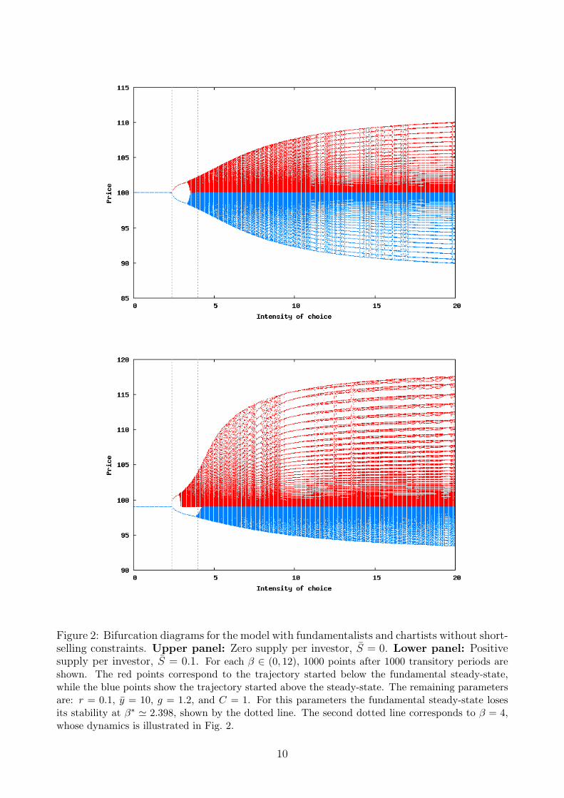
Figure 2: Bifurcation diagrams for the model with fundamentalists and chartists without short-selling constraints. Upper panel: Zero supply per investor, S = 0. Lower panel: Positivesupply per investor, S = 0.1. For each β ∈ (0, 12), 1000 points after 1000 transitory periods areshown. The red points correspond to the trajectory started below the fundamental steady-state,while the blue points show the trajectory started above the steady-state. The remaining parametersare: r = 0.1, y = 10, g = 1.2, and C = 1. For this parameters the fundamental steady-state losesits stability at β∗ ' 2.398, shown by the dotted line. The second dotted line corresponds to β = 4,whose dynamics is illustrated in Fig. 2.
10

Proposition 3.1 is illustrated on the bifurcation diagrams on Fig. 2 both for the zero supplycase and for the positive supply case. Two colors of the bifurcation diagrams correspond todifferent attractors for the same intensity of choice, see caption.
For small β the fundamental steady-state is globally stable. At this steady-state, the pre-cost performances of both types are the same, and the positions of all the agents are identicaland equal to S. However, the agents are distributed unevenly, with n∗2 > 1/2 > n∗1, due tothe positive costs paid by fundamentalists. The fundamental steady-state loses stability, whenthe intensity of choice is high enough. The precise bifurcation scenario depends on S. Whenthe supply is zero the stability is lost through the pitchfork bifurcation. For some range ofparameters β ∈ (β∗, β∗∗) the two symmetric, non-fundamental steady-states exist, so that thesystem converges to one of them, depending on the initial conditions. They simultaneously losetheir stability at β = β∗∗, and for the higher intensity of choice the oscillations with growingamplitudes persist. When the supply is positive, the two non-fundamental steady-states,stable and unstable, emerge through the saddle-node bifurcation for βsn < β∗. At β = β∗ thefundamental steady-state loses its stability through the transcritical bifurcation and if S isnot too high there exists some parameter range for which both non-fundamental steady-statesare locally stable. When β increases further, both these steady-states loses stability throughthe Neimark-Sacker bifurcation leading to the quasi-cyclic behavior.
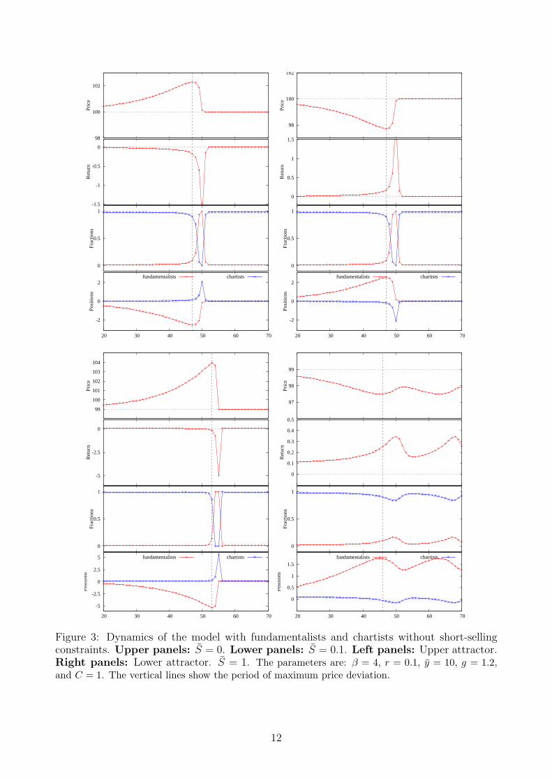
Notice that when β is relatively high, this model, even in its deterministic version, is able toreproduce the pattern of price bubbles and crashes. Consider the illustration of the dynamicsfor β = 4 in Fig. 3. Each of the four panels shows the evolution of price pt, return rt, fractionsof two types nt,h and positions of two types At,h.
Two upper panels correspond to the case of zero asset supply, S = 0. The upper leftpanel shows the dynamics at the upper attractor, when price is above pf = 100. In thefirst half of simulation the price is growing, but this growth is not sufficient to overcome therisk-free interest rate and the resulting return is eventually negative. The relative fraction ofchartists is high, because near the fundamental steady-state both types perform similarly, butfundamentalists pay the costs. Since the asset is overvalued, fundamentalists sell it, and thetrend-followers buy. Notice that the positions of two types are very different. Indeed, as agroup, fundamentalists hold short exactly the same amount of shares as chartists hold long.However, the relative fractions of two groups are very different and thus the per trader positionsof fundamentalists are much larger (in absolute value) than the per trader position of chartists.This asymmetry will have important consequences when short-sell constraints are introduced.The nature of crash is well-understood in this model. First of all, recall that we consider thecase of moderately extrapolating trend-followers. It guarantees that at a certain point alongthe bubble, the capital gain is not sufficient to overcome the negative effect of asset overpricingon the excess return (see (2.7)), and so the total return becomes negative. Second, when thereturn is negative, the positive fundamentalists’ pre-cost performance is clearly better thanthe negative performance of chartists. Therefore, the proportion of fundamentalists increases,slowing the price growth and decreasing the return even further.6 Due to the feedback of themodel, this effect is self-fulfilling. Eventually it leads to a relatively fast market crash, whenthe fundamentalists outperform chartists so significantly that they temporarily dominate themarket. The story then repeats itself.
The upper right panel shows the dynamics near the lower attractor, where the asset is
6Without taking the capital gain into account, the higher is the price, the smaller is the return, and alsothe bigger is the short position of fundamentalists, see (2.8). If the return is negative, both these effects workin favor of fundamentalists by increasing performance of this group.
11
-2
0
2
20 30 40 50 60 70
Posi
tions
fundamentalists chartists
0
0.5
1
Frac
tions
-1.5
-1
-0.5
0
Ret
urn
98
100
102Pr
ice
-2
0
2
20 30 40 50 60 70
Posi
tions
fundamentalists chartists
0
0.5
1
Frac
tions
0
0.5
1
1.5
Ret
urn
98
100
102
Pric
e
-5
-2.5
0
2.5
5
20 30 40 50 60 70
Posi
tions
fundamentalists chartists
0
0.5
1
Frac
tions
-5
-2.5
0
Ret
urn
99
100
101
102
103
104
Pric
e
0
0.5
1
1.5
20 30 40 50 60 70
Posi
tions
fundamentalists chartists
0
0.5
1
Frac
tions
0
0.1
0.2
0.3
0.4
0.5
Ret
urn
97
98
99
Pric
e
Figure 3: Dynamics of the model with fundamentalists and chartists without short-sellingconstraints. Upper panels: S = 0. Lower panels: S = 0.1. Left panels: Upper attractor.Right panels: Lower attractor. S = 1. The parameters are: β = 4, r = 0.1, y = 10, g = 1.2,and C = 1. The vertical lines show the period of maximum price deviation.
12
undervalued. The situation is symmetric with respect to the upper attractor, and the negativebubble is observed. The only important difference is that now, the stabilizing part of thepopulation (fundamentalists) are long in the risky asset.
Two lower panels show the dynamics in the case of positive asset supply for the samevalue of the intensity of choice, β = 4. On the upper attractor, shown in the lower leftpanel, the situation is similar to the zero supply case: the bubble pattern of growing price isfollowed by a short period of crash. Notice, however, the effect of positive supply on differentvariables. The return depends positively on the supply and during the bubble it remainspositive for a long time. Since fundamentalists take a short position, their performance isactually much worse than of trend-followers. However, once again the extrapolating effectof trend-followers is not sufficient to keep price growing. When the return becomes negativethe crash is inevitable: the fundamentalists with their large short positions get high return,increase their proportion, slow the price growth even further, and eventually overcome themarket. On the lower attractor, shown in the right lower panel, the dynamics is also similar tothe zero supply case.7 The symmetry with respect to the upper attractor, which was observedin zero supply case, is not present any longer. The reason lies in the effect of the positivesupply on the return. According to (2.7) the return increases with the supply, and on theupper attractor it temporarily prevented the fundamentalists from playing sufficient role tostabilize market. But on the lower attractor, to the contrary, higher return plays a positiverole. The fundamentalists who hold the positive positions get higher performance with higherreturns, helping market to stabilize faster. This also explains the peculiar difference betweentwo bifurcation diagrams shown in Fig. 2. Namely, controlling for the intensity of choice, theamplitude of oscillations of the positive bubbles is larger for positive supply case than for zerosupply case, and the opposite situation is observed for the lower attractor. Ceteris paribusthe positive supply increases return, which, given their relative positions, favors destabilizingchartists on the upper attractor and stabilizing fundamentalists on the lower attractor.
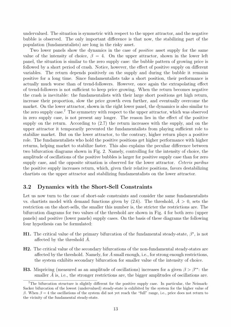
3.2 Dynamics with the Short-Sell Constraints
Let us now turn to the case of short-sale constraints and consider the same fundamentalistsvs. chartists model with demand functions given by (2.6). The threshold, A > 0, sets therestriction on the short-sells, the smaller this number is, the stricter the restrictions are. Thebifurcation diagrams for two values of the threshold are shown in Fig. 4 for both zero (upperpanels) and positive (lower panels) supply cases. On the basis of these diagrams the followingfour hypothesis can be formulated:
H1. The critical value of the primary bifurcation of the fundamental steady-state, β∗, is notaffected by the threshold A.
H2. The critical value of the secondary bifurcations of the non-fundamental steady-states areaffected by the threshold. Namely, for A small enough, i.e., for strong enough restrictions,the system exhibits secondary bifurcation for smaller value of the intensity of choice.
H3. Mispricing (measured as an amplitude of oscillations) increases for a given β > β∗∗: thesmaller A is, i.e., the stronger restrictions are, the bigger amplitudes of oscillations are.
7The bifurcation structure is slightly different for the positive supply case. In particular, the Neimark-Sacker bifurcation of the lowest (undervalued) steady-state is exhibited by the system for the higher value ofβ. When β = 4 the oscillations of the system did not yet reach the “full” range, i.e., price does not return tothe vicinity of the fundamental steady-state.
13

Figure 4: Bifurcation diagrams for the model with fundamentalists and chartists with short-selling constraints. Upper panels: Zero supply per investor, S = 0. Lower panels: Positivesupply per investor, S = 0.1. Left panels: A = 2. Right panels: More stringent constraint,A = 1. For each β ∈ (0, 12), 1000 points after 1000 transitory periods are shown. The red pointscorrespond to the trajectory started below the fundamental steady-state, while the blue points showthe trajectory started above the steady-state. The remaining parameters are: r = 0.1, y = 10,g = 1.2, and C = 1.
H4. A symmetry between upper and lower attractors breaks down also for the zero supplycase: the positive bubbles have bigger amplitudes.
These four hypothesis turns out to be correct. Below we provide a heuristic proof for thesehypothesis and extend their validity for other ecologies.
Hypotheses H1 and H2: Short-sell Constraints and Local Stability
The first hypothesis says that the stability properties of the fundamental steady-state are inde-pendent from the constraints. The result holds, because the positions of both fundamentalistsand chartists at the fundamental steady-state are equal to S ≥ 0. Thus, the short-sell con-straints with positive threshold are never binding, and do not affect the local stability of thesteady-state. In other words, the short-selling restrictions can neither stabilize nor destabilizethe market, in the sense that they do not affect the value of bifurcation of the fundamental
14
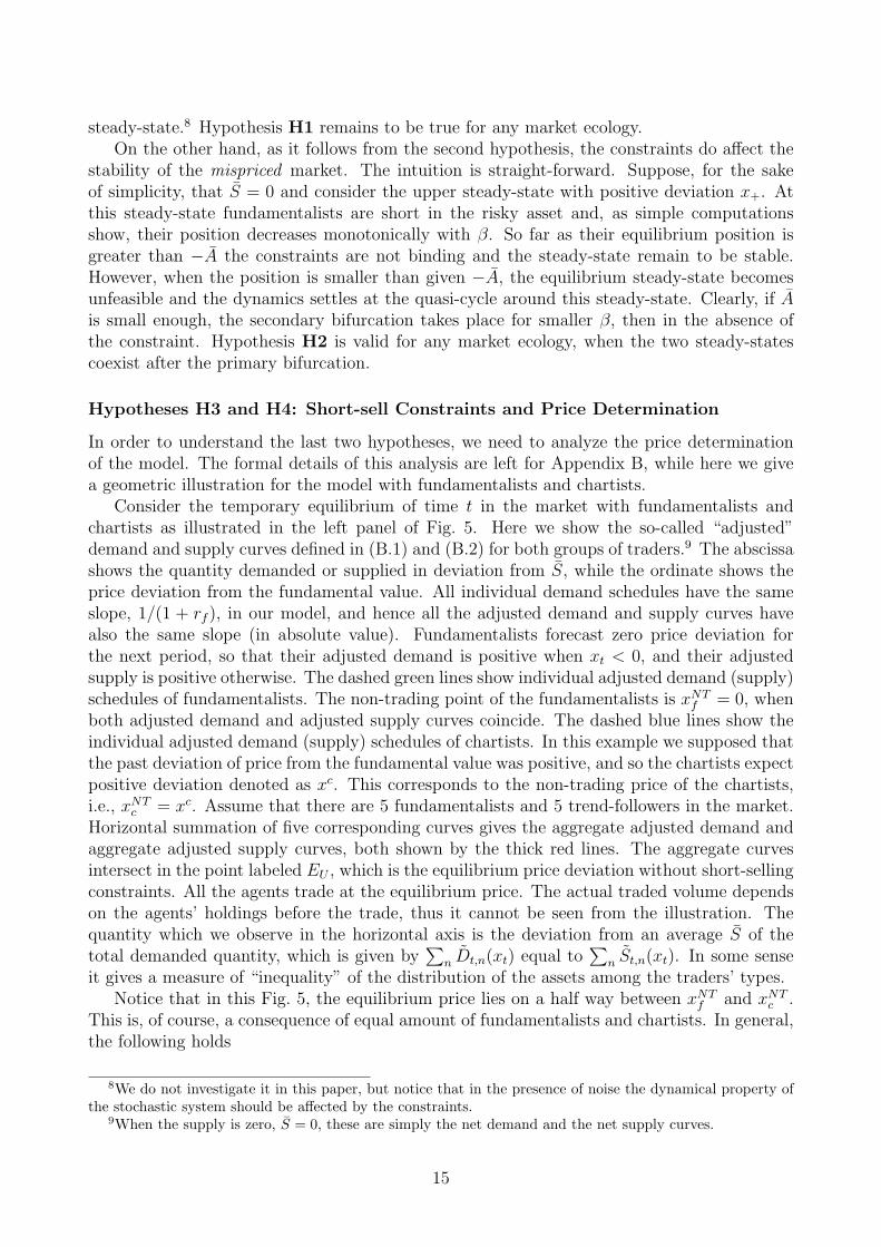
steady-state.8 Hypothesis H1 remains to be true for any market ecology.On the other hand, as it follows from the second hypothesis, the constraints do affect the
stability of the mispriced market. The intuition is straight-forward. Suppose, for the sakeof simplicity, that S = 0 and consider the upper steady-state with positive deviation x+. Atthis steady-state fundamentalists are short in the risky asset and, as simple computationsshow, their position decreases monotonically with β. So far as their equilibrium position isgreater than −A the constraints are not binding and the steady-state remain to be stable.However, when the position is smaller than given −A, the equilibrium steady-state becomesunfeasible and the dynamics settles at the quasi-cycle around this steady-state. Clearly, if Ais small enough, the secondary bifurcation takes place for smaller β, then in the absence ofthe constraint. Hypothesis H2 is valid for any market ecology, when the two steady-statescoexist after the primary bifurcation.
Hypotheses H3 and H4: Short-sell Constraints and Price Determination
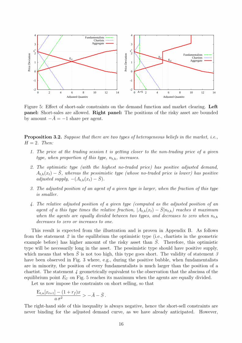
In order to understand the last two hypotheses, we need to analyze the price determinationof the model. The formal details of this analysis are left for Appendix B, while here we givea geometric illustration for the model with fundamentalists and chartists.
Consider the temporary equilibrium of time t in the market with fundamentalists andchartists as illustrated in the left panel of Fig. 5. Here we show the so-called “adjusted”demand and supply curves defined in (B.1) and (B.2) for both groups of traders.9 The abscissashows the quantity demanded or supplied in deviation from S, while the ordinate shows theprice deviation from the fundamental value. All individual demand schedules have the sameslope, 1/(1 + rf ), in our model, and hence all the adjusted demand and supply curves havealso the same slope (in absolute value). Fundamentalists forecast zero price deviation forthe next period, so that their adjusted demand is positive when xt < 0, and their adjustedsupply is positive otherwise. The dashed green lines show individual adjusted demand (supply)schedules of fundamentalists. The non-trading point of the fundamentalists is xNTf = 0, whenboth adjusted demand and adjusted supply curves coincide. The dashed blue lines show theindividual adjusted demand (supply) schedules of chartists. In this example we supposed thatthe past deviation of price from the fundamental value was positive, and so the chartists expectpositive deviation denoted as xc. This corresponds to the non-trading price of the chartists,i.e., xNTc = xc. Assume that there are 5 fundamentalists and 5 trend-followers in the market.Horizontal summation of five corresponding curves gives the aggregate adjusted demand andaggregate adjusted supply curves, both shown by the thick red lines. The aggregate curvesintersect in the point labeled EU , which is the equilibrium price deviation without short-sellingconstraints. All the agents trade at the equilibrium price. The actual traded volume dependson the agents’ holdings before the trade, thus it cannot be seen from the illustration. Thequantity which we observe in the horizontal axis is the deviation from an average S of thetotal demanded quantity, which is given by
∑n Dt,n(xt) equal to
∑n St,n(xt). In some sense
it gives a measure of “inequality” of the distribution of the assets among the traders’ types.Notice that in this Fig. 5, the equilibrium price lies on a half way between xNTf and xNTc .
This is, of course, a consequence of equal amount of fundamentalists and chartists. In general,the following holds
8We do not investigate it in this paper, but notice that in the presence of noise the dynamical property ofthe stochastic system should be affected by the constraints.
9When the supply is zero, S = 0, these are simply the net demand and the net supply curves.
15
-2
-1
0
1
2
3
4
0 2 4 6 8 10 12 14
Pric
e D
evia
tion
Adjusted Quantity
EU
xc
FundamentalistsChartists
Aggregate
-2
-1
0
1
2
3
4
0 2 4 6 8 10 12 14
Pric
e D
evia
tion
Adjusted Quantity
EU
EC
xc
A+S
FundamentalistsChartists
Aggregate
Figure 5: Effect of short-sale constraints on the demand function and market clearing. Leftpanel: Short-sales are allowed. Right panel: The positions of the risky asset are boundedby amount −A = −1 share per agent.
Proposition 3.2. Suppose that there are two types of heterogeneous beliefs in the market, i.e.,H = 2. Then:
1. The price at the trading session t is getting closer to the non-trading price of a giventype, when proportion of this type, nt,h, increases.
2. The optimistic type (with the highest no-traded price) has positive adjusted demand,At,h(xt) − S, whereas the pessimistic type (whose no-traded price is lower) has positiveadjusted supply, −(At,h(xt)− S).
3. The adjusted position of an agent of a given type is larger, when the fraction of this typeis smaller.
4. The relative adjusted position of a given type (computed as the adjusted position of anagent of a this type times the relative fraction, |At,h(xt) − S|nt,h) reaches it maximumwhen the agents are equally divided between two types, and decreases to zero when nt,hdecreases to zero or increases to one.
This result is expected from the illustration and is proven in Appendix B. As followsfrom the statement 2 in the equilibrium the optimistic type (i.e., chartists in the geometricexample before) has higher amount of the risky asset than S. Therefore, this optimistictype will be necessarily long in the asset. The pessimistic type should have positive supply,which means that when S is not too high, this type goes short. The validity of statement 3have been observed in Fig. 3 where, e.g., during the positive bubble, when fundamentalistsare in minority, the position of every fundamentalists is much larger than the position of achartist. The statement 4 geometrically equivalent to the observation that the abscissa of theequilibrium point EU on Fig. 5 reaches its maximum when the agents are equally divided.
Let us now impose the constraints on short selling, so that
Et,n[xt+1]− (1 + rf )x
a σ2> −A− S .
The right-hand side of this inequality is always negative, hence the short-sell constraints arenever binding for the adjusted demand curve, as we have already anticipated. However,
16
they are binding on the adjusted supply curve, which becomes inelastic at quantity A + Sas illustrated in the right panel of Fig. 5.10 Any individual adjusted supply curve becomesvertical when
xt =Et,n[xt+1] + aσ2(A+ S)
1 + rf.
Imposed short-sell constraints change the aggregate supply schedule, as well as the equilibriumpoint EC . In this example the equilibrium price under short-selling constraints is larger thanthe equilibrium price without constraints, while the quantity traded is smaller. Such outcomeis expected, given Proposition 3.2. Fundamentalists represent a pessimistic type, and for themthe constraints are binding. Since supply is restricted, the price goes up.
Now the hypotheses H3 and H4 formulated above become obvious. When the short-sell constraints are imposed, and the dynamics follow the positive trend, the fundamentalistsare short. The equilibrium level of price at a given period becomes higher due to insufficientliquidity. Such an effect is well understood in the theoretical literature on short-selling at leastsince Miller (1977). In our model, however, there are also dynamic consequences. The higherprice growth rate (with respect to the no-constrained benchmark model) has a positive impacton the return. At the same time, the fundamentalists are restricted in their negative positions.Both these factors contribute to worsening the performance of fundamentalists. Consequently,the mispricing will be larger at the next period, and even larger if the constraints are imposedat that period as well. Overall, the bubble can last longer. It explains hypothesis H3.
Finally, there exists an asymmetry on the impact of the short-selling constraints betweendynamics on the upper and on the lower attractors. In both cases chartists dominate themarket, but on the upper attractor their type dominates, while and on the lower attractor theother type dominates. Part 3 of Proposition 3.2 implies that the same constraints are morebinding for the type which is in minority. It means that the constraint will always have largerconsequences for the dynamics on the upper attractor. In particular, it explains hypothesisH4, that is the symmetry breaking in the zero supply case.
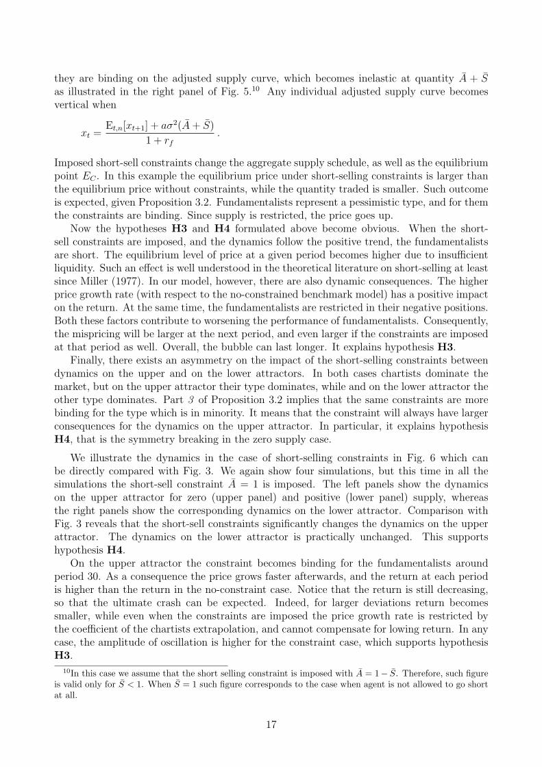
We illustrate the dynamics in the case of short-selling constraints in Fig. 6 which canbe directly compared with Fig. 3. We again show four simulations, but this time in all thesimulations the short-sell constraint A = 1 is imposed. The left panels show the dynamicson the upper attractor for zero (upper panel) and positive (lower panel) supply, whereasthe right panels show the corresponding dynamics on the lower attractor. Comparison withFig. 3 reveals that the short-sell constraints significantly changes the dynamics on the upperattractor. The dynamics on the lower attractor is practically unchanged. This supportshypothesis H4.
On the upper attractor the constraint becomes binding for the fundamentalists aroundperiod 30. As a consequence the price grows faster afterwards, and the return at each periodis higher than the return in the no-constraint case. Notice that the return is still decreasing,so that the ultimate crash can be expected. Indeed, for larger deviations return becomessmaller, while even when the constraints are imposed the price growth rate is restricted bythe coefficient of the chartists extrapolation, and cannot compensate for lowing return. In anycase, the amplitude of oscillation is higher for the constraint case, which supports hypothesisH3.
10In this case we assume that the short selling constraint is imposed with A = 1− S. Therefore, such figureis valid only for S < 1. When S = 1 such figure corresponds to the case when agent is not allowed to go shortat all.
17
-2
0
2
20 30 40 50 60 70
Posi
tions
fundamentalists chartists
0
0.5
1
Frac
tions
-1.5
-1
-0.5
0
Ret
urn
98
100
102Pr
ice
-2
0
2
20 30 40 50 60 70
Posi
tions
fundamentalists chartists
0
0.5
1
Frac
tions
0
0.5
1
1.5
Ret
urn
98
100
102
Pric
e
-5
-2.5
0
2.5
5
20 30 40 50 60 70
Posi
tions
fundamentalists chartists
0
0.5
1
Frac
tions
-5
-2.5
0
Ret
urn
99
100
101
102
103
104
Pric
e
0
0.5
1
1.5
20 30 40 50 60 70
Posi
tions
fundamentalists chartists
0
0.5
1
Frac
tions
0
0.1
0.2
0.3
0.4
0.5
Ret
urn
97
98
99
Pric
e
Figure 6: Dynamics of the model with fundamentalists and chartists with short-selling con-straints A = 1. Upper panels: S = 0. Lower panels: S = 0.1. Left panels: Upperattractor. Right panels: Lower attractor. S = 1. The parameters are: β = 4, r = 0.1, y = 10,g = 1.2, and C = 1. The vertical lines show the period of maximum price deviation for dynamicswithout constraints, see Fig. 3.
18
0
20
40
60
20 30 40 50 60 70 80 90 100
Posi
tions
fundamentalists chartists
0
0.5
1
Frac
tions
-50
-30
-10
Ret
urn
100
120
140
160
Pric
e
0
20
40
60
20 30 40 50 60 70 80 90 100
Posi
tions
fundamentalists chartists
0
0.5
1
Frac
tions
-50
-30
-10
Ret
urn
100
120
140
160
Pric
e
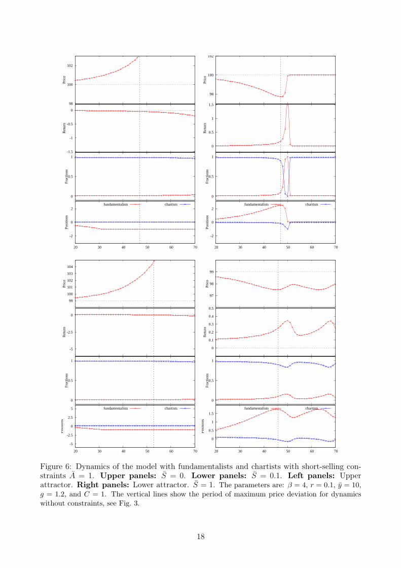
Figure 7: Crash of the market with fundamentalists and chartists with short-selling constraintsA = 1. Left panel: S = 0. Right panel: S = 0.1. The parameters are: β = 4, r = 0.1, y = 10,g = 1.2, and C = 1. The vertical lines show the period of maximum price deviation for dynamicswithout constraints, see Fig. 3.
The dynamics on the lower attractor is always unaffected by the constraints. For examplefor the positive supply case (lower right panel) the constraints are never binding. The chartistsare short in the asset and they represent the majority in the market. Consequently, the positionof every of them is relatively high. Actually, the lowest position per chartist is observed afterthe negative bubble “crashes”, when the population of chartists shrinks. For the zero supplycase (upper right panel) this is a unique moment when the constraints are binding. When theconstraints are imposed the fundamentalists represent even larger population than withoutconstraints, which helps market to correct faster.
Let us now return to the upper attractor and consider the effects of the constraints onthe crash, see Fig. 7. The left panel illustrates the case of zero supply and the right panelillustrates the case of positive supply. In both cases the crash occurs much later than in thecase of no-constraints (compare two horizontal lines indicating the maximum price deviation).The constraints do not prevent the crash, but as a consequence of the constraints the crashis much more pronounce, and is characterized by the lower return. The evolution of fractionsshows that much larger relative fraction of fundamentalists is needed to stop the price growth.
The analysis above also suggests how the dynamics is affected by parameters A and S.Return to Fig. 5 and notice that increase in the assets’ supply and increase of the thresholdA (i.e., relaxing the constraints) have equal effects on the geometry of restrictions. In bothcases the inelastic part of supply curve shifts right. Effectively, an increase of the total supplymakes the constraints less strict. The amplitude of dynamics will decrease in this case given β.
19

Indeed, comparing Figs. 7 and 3 one can see that equal amount of the short-selling constraintsleads to relatively bigger increase in amplitude of oscillations for the zero supply case.
4 Managing Price Dynamics by Short-Selling Constraints
In the previous Section we have established two important results. On the one hand, we havefound the short-selling constraints do not matter for the intensity of choice smaller than thebifurcation value of the fundamental steady-state. On the other hand, we have found thatafter the bifurcation, the amplitude of oscillations increases. For such values of the intensityof choice, the short-sell constraints destabilize dynamics.
One can now ask, however, what would the effects of the constraints be, if they wouldbe imposed only on the downward part of the price dynamics. This would be similar to thethree weeks short-sell ban imposed in October 2008, as it was discussed in the Introduction.Furthermore, in the example of Section 3, the chartists did not extrapolate the trend, and sothey could not potentially worsen the crash of the market. Motivated by these remarks wewill consider now the model with alternative two types of traders.
The fundamentalists have the rule
Et,1[pt+1] = pf + v (pt−1 − pf ) , v ∈ [0, 1] , (4.1)
which is similar to (3.1). Fundamentalists predict that any price deviation from the funda-mental level will be (partially) corrected. In one limiting case, v = 0, immediate correction isexpected, while in another limiting case, v = 1, agents rely on the market, expecting that thelast observed price is the best predictor. The trend-following forecasting rule
Et,2[pt+1] = pt−1 + g (pt−1 − pt−2) , g > 0 , (4.2)
predicts that past trends in the price will hold. It extrapolates the past trend with coefficientg. Notice that the fundamental forecasting rule (as opposed to the trend-following forecastingrule) requires a knowledge of fundamental value. Consequently, we assume that to use thefundamental rule the agent has to pay cost C > 0 per period, whereas the second rule isavailable for free.
In the absence of the short-sell constraints the model is described by one equation of thefourth order (or, equivalently by the 4-dimensional system) consisting of the market clearingequation coupled with an update of the fractions of fundamentalists:
xt+1 =1
R
(vxt n1,t+1 +
(xt + g(xt − xt−1)
)(1− n1,t+1)
)+ εt+1
n1,t+1 = exp
(β
[(v xt−2 −Rxt−1
aσ2+ s
) (xt −Rxt−1 + δt + aσ2s
)− C
])/Zt+1
, (4.3)
where normalization factor
Zt+1 = exp(β(U1,t − C)
)+ exp
(βU2,t
)=
= exp
(β
[(v xt−2 −Rxt−1
aσ2+ s
) (xt −Rxt−1 + δt + aσ2s
)− C
])+
+ exp
(β
(xt−2 + g(xt−3 − xt−2)−Rxt−1
aσ2+ s
) (xt −Rxt−1 + δt + aσ2s
)).
(4.4)
20
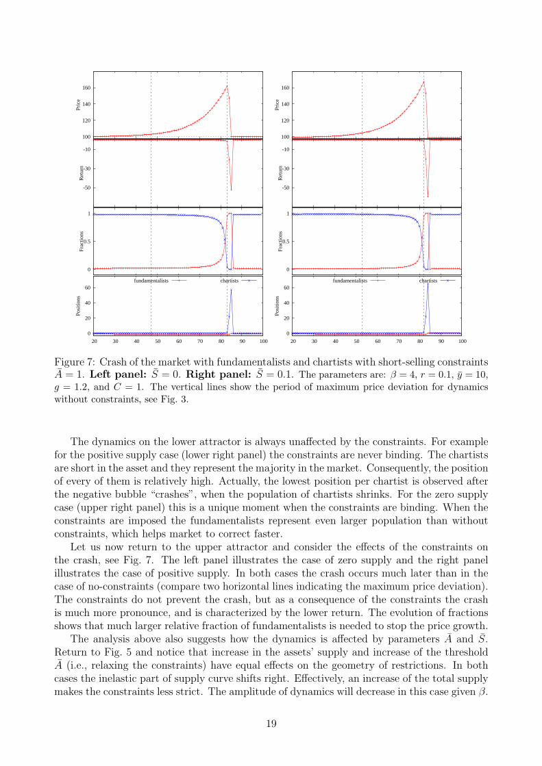
Figure 8: Bifurcation diagrams for the fundamentalists vs. trend-followers model. Left panel:Short-selling constraints are not imposed. Right panel: Short-selling constraints with A =0.5 are imposed (red) compared with the no-constraints case (blue). For each β ∈ (0, 20), 1000points after 1000 transitory periods are shown. Parameters are: r = 0.1, y = 10, v = 0.1, g = 1.2,C = 1 and S = 0.
When g > 1 + rf , this system has two possible dynamics as function of the intensity of choice.When the intensity of choice β is low, the fundamental steady-state is locally stable. Thissteady-state loses stability, and for higher intensity of choice the oscillations persist.
Fig. 8 compares the bifurcation diagrams without and with short-selling constraints. Evenif the structure of the dynamics is different with respect to the model in Section 3, the effect ofshort-sell constraints is the same. Also in this “fundamentalists vs. trend-followers” model theshort-sell constraints leads to larger amplitude of fluctuations. The main reason of such largeramplitude is the limitation of fundamentalists in the mispricing correction. The situation isalso illustrated in the left panel of Fig. 9. There we show how the price dynamics changes whenthe short-sell constraints are imposed at a period t = 40, when the market is on the upwardpart of the price trend. Similarly to the previous model, fundamentalists are constrained andthe bubble can last longer.
Now suppose that the constraints are introduced on the downward part of dynamics. Thesimulation in the right panel of Fig. 9 shows that the market crash, indeed, slows with thehelp of the constraints. However, the lowest point of the price dynamics is not changing. Inother words, the constraints does not allow to avoid the crash.
5 Conclusion
In this paper we have analyzed the quantitative consequences of the short-selling constraintsfor the asset-pricing dynamics. Existing literature mostly points out that the short-sellingrestrictions can lead to systematic overvaluation of the security. The intuition for that wasprovided by Miller (1977) who shows, in the two-period setting, that a diversity of expectationsamong investors leads to overpricing. Our model formalizes this intuition and extends it for adynamical setting.
In our model demand of myopic investors depends on their expectations of future price. Theexpectations are heterogeneous and agents are allowed to switch between different forecastingrules over time. As it is well known, the dynamics of such model depends on the intensity of
21

95
100
105
110
115
120
125
130
0 20 40 60 80 100
contsrained at t = 40, A = 7no constraints
95
100
105
110
115
120
125
130
0 20 40 60 80 100
contsrained at t = 40, A = 7constrained at t = 50, A = 5
no constraints
Figure 9: Price dynamics in the fundamentalists vs. trend-followers model. Left panel: Pricedynamics without constraints (blue) is compared with price dynamics when the short-sellingconstraints with A = 7 are imposed at period t = 40 (red). Right panel: The same pricedynamics are compared with price dynamics when the short-selling constraints with A = 5are imposed at period t = 50 (purple). Parameters are: r = 0.1, y = 10, v = 0.1, g = 1.2,C = 1 and S = 0.
choice. For low values of this parameter the dynamics converge to the fundamental steady-state. When the constraints are introduced in this scenario, the local dynamics will notchange, since the constraints will never be binding in the steady-state. For high values of theintensity of choice dynamics do not converge to the fundamental steady-state. Instead, themodel exhibits price oscillations with excess volatility. The relevance of short-sell constraintsis especially important for the dynamics of such scenario.
It turns out that the constraints increase volatility of the price. This is the outcome of twoeffects, liquidity effect, which limits the stabilizing force of those traders whose evaluations arethe closest to the fundamental value, and market ecology effect, according to which the perfor-mance of such stabilizing traders is getting worse when the short-sell constraints are imposed,and consequently more time is needed for the market correction. As a result, inevitable crashis more severe in the presence of the short-sell constraints. We have also investigated the con-sequence of the restrictions introduced along the downward price trend, when the constrainedinvestors are the destabilizing trend-followers. Similarly to the dynamics observed during 2008market crash, such constraints would slow the downward price movement, but would not stopit.
To study the effect of short-sell constraints, we have deliberately chosen a model withheterogeneous expectations, capable to generate the patterns of bubbles and crashes. Somefeatures of this model may however, influence our findings. Consequently, in the future researchwe would like to extend the model in different directions. First, the myopic agents of the modeldo not take the short-sell constraints into account while forming their expectations. Whilewe believe that such assumption is quite reasonable in the framework of boundedly rationalagents, it would be also interesting to analyze the model with some fraction of rational agents,who take the short-sell constraints into account. Second, the constraints which we analyzedwere individual, while on the real markets there are many aggregate constraints. For example,a total amount of shares available for the short sales is, in reality, limited. The effect ofsuch types of constraint can be analyzed within the agent-based version of the model outlinedin Appendix A. Finally, the effect of short selling constraints is closely related to the role
22

of margin requirements. Indeed, in a real market selling a share short requires providingsome collateral to the broker. If the price of an asset rises, the investor who is short shouldcover his nominal losses to the extent which depends on the margin requirement. It is notsurprising that among the most important questions discussed in the literature on marginalrequirement is their role in market volatility and preventing bubbles. Two opposing points ofviews can be found in the literature on margin requirements. On the one hand, Seguin andJarrell (1993) and Hsieh and Miller (1990) argue that margin requirements are empiricallyirrelevant for price behavior, whereas, e.g., Garbade (1982) and Hardouvelis and Theodossiou(2002) provide theoretical arguments why an increase in margin requirements is beneficial formarket stability. Again, with the agent-based extension of the model presented here we planto analyze the joint effect of short-sell constraints and market requirements on the dynamics.
References
Anderson, S., A. de Palma, and J.-F. Thisse (1992): Discrete Choice Theory of ProductDifferentiation. MIT Press, Cambridge, MA.
Anufriev, M., and V. Panchenko (2009): “Asset Prices, Traders’ Behavior and MarketDesign,” Journal of Economic Dynamics & Control, 33, 1073 – 1090.
Barberis, N., and R. Thaler (2003): “A Survey of Behavioral Finance,” in Handbookof the Economics of Finance, ed. by G. Constantinides, M. Harris, and R. Stultz. North-Holland (Handbooks in Economics Series), Amsterdam.
Brock, W. (1993): “Pathways to randomness in the economy: Emergent nonlinearity andchaos in economics and finance,” Estudios Economicos, 8, 3–55.
Brock, W. A., and C. H. Hommes (1997): “A Rational Route to Randomness,” Econo-metrica, 65(5), 1059–1095.
(1998): “Heterogeneous Beliefs and Routes to Chaos in a Simple Asset PricingModel,” Journal of Economic Dynamics and Control, 22, 1235–1274.
Camerer, C. F., and T.-H. Ho (1999): “Experienced-Weighted Attraction Learning inNormal Form Games,” Econometrica, 67(4), 827–874.
Diamond, D., and R. Verrecchia (1987): “Constraints on short-selling and asset priceadjustment to private information,” Journal of Financial Economics, 18(2), 277–311.
Evans, G. W., and S. Honkapohja (2001): Learning and Expectations in Macroeconomics.Princeton University Press.
Galbraith, J. (1954): The Great Crash, 1929.
Gallmeyer, M., and B. Hollifield (2008): “An Examination of Heterogeneous Beliefswith a Short-Sale Constraint in a Dynamic Economy,” Review of Finance.
Garbade, K. (1982): “Federal Reserve margin requirements: A regulatory initiative toinhibit speculative bubbles,” Crises in the Economic and Financial Structure, pp. 317–36.
23

Gaunersdorfer, A., and C. Hommes (2007): “A Nonlinear Structural Model for VolatilityClustering,” in Long Memory in Economics, ed. by G. Teyssiere, and A. Kirman, pp. 265–288. Springer.
Hardouvelis, G., and P. Theodossiou (2002): “The asymmetric relation between initialmargin requirements and stock market volatility across bull and bear markets,” Review ofFinancial Studies, 15(5), 1525 – 1560.
Harrison, J., and D. Kreps (1978): “Speculative investor behavior in a stock market withheterogeneous expectations,” The Quarterly Journal of Economics, pp. 323–336.
Haruvy, E., and C. Noussair (2006): “The effect of short seliing on bubbles and crashesin experimental spot asset markets,” Journal of Finance, 61(3), 1119–1157.
Hommes, C. (2006): “Heterogeneous Agent Models in Economics and Finance,” in Hand-book of Computational Economics Vol. 2: Agent-Based Computational Economics, ed. byK. Judd, and L. Tesfatsion. Elsevier/North-Holland (Handbooks in Economics Series).
Hommes, C., H. Huang, and D. Wang (2005): “A robust rational route to randomness ina simple asset pricing model,” Journal of Economic Dynamics and Control, 29, 1043–1072.
Hommes, C., J. Sonnemans, J. Tuinstra, and H. v. d. Velden (2005): “Coordinationof Expectations in Asset Pricing Experiments,” Review of Financial Studies, 18(3), 955–980.
Hsieh, D., and M. Miller (1990): “Margin requirements and market volatility,” Journalof Finance, 45.
Jones, C., and O. Lamont (2002): “Short-sale constraints and stock returns,” Journal ofFinancial Economics, 66(2-3), 207–239.
Lamont, O., and R. Thaler (2003): “Can the market add and subtract? Mispricing intech stock carve-outs,” Journal of Political Economy, 111(2), 227–268.
LeBaron, B. (2006): “Agent-Based Computational Finance,” in Handbook of ComputationalEconomics Vol. 2: Agent-Based Computational Economics, ed. by K. Judd, and L. Tesfat-sion. Elsevier/North-Holland (Handbooks in Economics Series).
Lecce, S., A. Lepone, and R. Segara (2008): “The impact of naked short-sales on returns,volatility and liquidity: evidence from the Australian Securities Exchange,” 21st australasianfinance and banking conference 2008 paper, http://ssrn.com/abstract=1253176.
Lei, V., C. Noussair, and C. Plott (2001): “Nonspeculative bubbles in experimentalasset markets: lack of common knowledge of rationality vs. actual irrationality,” Economet-rica, pp. 831–859.
Lux, T. (2009): “Stochastic Behavioral Asset Pricing Models and the Stylized Facts,” Hand-book of Financial Markets: Dynamics and Evolution, p. 161.
Miller, E. M. (1977): “Risk, uncertainty, and divergence of opinion,” Journal of Finance,32, 1151–1168.
Seguin, P., and G. Jarrell (1993): “The irrelevance of margin: Evidence from the Crashof ’87,” Journal of Finance, pp. 1457–1473.
24

Setzu, A., and M. Marchesi (2008): “The effect of short-selling and margin trading: asimulation analysis,” Discussion paper, CiteSeerX.
Shleifer, A. (2000): Inefficient markets: An introduction to behavioral finance. OxfordUniversity Press.
Smith, V. L., G. L. Suchanek, and A. W. Williams (1988): “Bubbles, Crashes, andEndogenous Expectations in Experimental Spot Asset Markets,” Econometrica, 56(5), 1119–1151.
Weisbuch, G., A. Kirman, and D. Herreiner (2000): “Market Organisation and TradingRelationships,” Economic Journal, 110, 411–436.
25

APPENDIX
A Agent-Based Version of the Model
Denote the trader with sub-index n ∈ {1, . . . , N} and consider the evolution of the trader’s position.Assume that agent n after the trading session at time t has At,n shares of the risky asset and Bt,n ofthe numeraire (i.e., the riskless assets). The wealth of investor at the end of the period is then givenby
Wt,n = Bt,n + ptAt,n .
In the beginning of the next period agent receives a dividend yt+1 for the every share of the risky assetand the interest on the riskless possession. We assume that agent does not consume and receives allthe payments in terms of numeraire. In addition, the agent trades at period t+ 1 and his position inthe risky asset after the trade is given by At+1,n shares. The trade balance is also received in termsof numeraire. Simple accounting implies that
Bt+1,n = (1 + rf )Bt,n + yt+1At,n + pt+1At,n − pt+1At+1,n , (A.1)
where the penultimate term in the RHS shows revenue from selling the previous possessions onmarket prices, while the last term gives the spending on the new shares. With simple algebra wederive the standard equation for wealth evolution
Wt+1,n = Bt+1,n + pt+1At+1,n == (1 + rf )Bt,n + yt+1At,n + pt+1At,n − pt+1At+1,n + pt+1At+1,n == (1 + rf )Bt,n +At,n(yt+1 + pt+1) == (1 + rf )Wt,n − (1 + rf )ptAt,n +At,n(yt+1 + pt+1) == (1 + rf )Wt,n +At,n(yt+1 + pt+1 − (1 + rf )pt) .
In the absence of short-selling and liquidity constraints, the mean-variance optimization problemgives us the demand function
At,n(p) =Et,n[pt+1] + y − (1 + rf )p
a σ2.
Notice that this is the same function as in (2.1), written for agent n of type h. The demand is adecreasing linear function of price, which represents an amount of shares an agent wishes to have atthe end of period t.
Depending on the market clearing mechanism the trader’s demand can be satisfied or the tradercan be rationed. For example, in the body of this paper we consider the evolution under Walrasianmarket clearing, when price pt is such that every agents’ demand is satisfied. Similarly, under MarketMaker Scenario a special agent, market-maker, quotes the price pt at the beginning of the day andevery trader’s position is given by his realized demand at this price. Thus in both cases
At,n = At,n(pt) =Et,n[pt+1] + y − (1 + rf )pt
a σ2.
Instead, rationing can occur in some circumstances, as, e.g., under the order-based market clearingmechanism as studied in Anufriev and Panchenko (2009). In the Walrasian market the rationing canalso occur if the short selling constraint should hold not individually, but in aggregate.
The choice of forecasting type by agent n is based upon the commonly observed deterministiccomponent reflecting the past performances of the rules and stochastic error component reflectingthe measurement error or imperfect computations of agents. The choice is modeled as follows. At
26
the end of trading round t, first, an individual realized excess profit is computed as a product ofholdings of the risky asset at the end of round t− 1 and its excess return, that is
At−1,n
(pt + yt − (1 + rf ) pt−1
). (A.2)
The position of agent At−1,n reflects the choice of the forecasting rule made before the t − 1-trade.Once individual profits have been computed, the performances of any rule, Ut,h, are defined as theaverages of the individual realized excess profits over all agents who used a given rule. From (A.2)it is clear that performance of the rule is the average holdings of the followers of this rule times theexcess return. Thus, if the risky asset has earned a positive (negative) return, then the performanceof the group with larger average possessions of the asset is higher (smaller).
Finally, agent n chooses the predictor for which the following maximum is realized
maxh
(Ut,h − Ch + ξt,n,h
),
where Ch is the cost of rule h, and ξt,n,h are random variables independent over agents and rules.The choice can be rewritten in terms of probabilities for the special case of a Gumbel distribution oferror terms. In this case, individual n chooses the predictors with discrete choice probabilities11
πh,t+1 =exp
(β(Uh,t − Ch)
)∑Hh′=1 exp
(β(Uh′,t − Ch′)
) . (A.3)
with a subscript indicating that these probabilities shape the population of trades at period t + 1.Parameter β ≥ 0 is the intensity of choice, which is inversely related to the variance of the noiseterm ξi,h,t.
Large Market Limit
We presented above our model in an agent-based way, so that one has to keep track on the positionof every agent to analyze the price dynamics. However, the dynamics can be considerably simpli-fied under certain conditions, and the “Large Market Limit” model in the main text of this paperrepresents such simplification.12 To derive the “Large Market Limit” recall that under Walrasianmarket-clearing the demand of every agent is satisfied, so that the individual positions At,n becomeidentical for all the agents with the same forecasting rule. The dimensionality of dynamics can bethen reduced by considering the level of forecasting rules instead of the agents’ level. This forecastingrule level was referred as “type” in the main text.
In the Walrasian framework the equilibrium price pt is the solution of the market clearing equa-tion:
N∑n=1
At,n(pt) = S . (A.4)
If we divide both parts of this equality on the number of agents, N , we obtain the same equilibriumequation in terms of fractions nt,h = Nt,h/N of investors using the rule h
H∑h=1
nt,hAt,h(p) = S .
11Our specification of the error terms is common in the literature on random utility models; see Anderson,de Palma, and Thisse (1992). Implied probabilities are used to model a choice in a number of theoreticalmodels with a different range of applications, see, e.g., Brock (1993), Brock and Hommes (1997), Camerer andHo (1999), and Weisbuch, Kirman, and Herreiner (2000).
12Essentially, the difference between agent-based approach as reviewed in LeBaron (2006) and HAMs asreviewed in Hommes (2006) lies in the dimensionality of dynamical systems, which are low in the latter case,even if agents’ heterogeneity is present.
27

This is the same equation as in (2.2). Now suppose that N →∞ and S →∞ in such a way that thesupply per investor, S = S/N , is constant. Then equation (2.2) gives the price dynamics. Further-more, as N becomes large, the probabilistic choice of the strategies as in (A.3) results, according tothe Law of Large Numbers, in the fraction of the type h equal to the probability. In other words,nh,t+1 = πh,t+1, which implies the evolution (2.4). Thus, the Large Market Model is obtained underWalrasian scenario, when the number of agents becomes large.
Notice, that the key assumption in simplification was that the demand of every trader is satisfied.Thus, one can also consider the Large Market Model under the market-maker scenario. In suchscenario, the market-maker adjusts price on the basis of the excess demand/supply. It leads to thefollowing (linear) adjustment rule
pt+1 = pt + µ( N∑n=1
At,n(pt)− S), (A.5)
where positive coefficient µ measures the speed of adjustment.13 Again, if N →∞ and S →∞ butthe ratio S = S/N is constant, then (A.5) becomes
pt+1 = pt + µ( H∑h=1
nt,hAt,h(pt)− S).
Further Directions of Research
In the text of Section 2 of the paper we have formulated five different objections for our research.Three of them can be successfully reached within the Large Market Limit, but the remaining twowould require the agent-based approach.
The fourth objective was to study consequences of the imperfection of the market for borrowingshares. Let us illustrate it with the following aggregate restriction∑
n:At,n<0
At,n ≥ −S , (A.6)
which says that the total amount of borrowed shares cannot exceed the total supply of shares. Whensuch restriction is violated at least some short-selling agents will fail to deliver. Therefore, imposinga restriction (A.6) can be interpreted as a ban on the naked short sellings. Of course, very strongshort sell restrictions (i.e., those with a very small A) will automatically rule out the naked shortsellings in this sense, but it also could be that every agent is allowed to go short to some extent (oruntil infinity) but aggregate restriction as (A.6) is imposed. Independent of how the agents’ rationingis modeled, the fulfillment of the 4th goal would clearly require an agent-based simulations.
The 5th objection refers on the borrowing constraints, which are symmetric with respect to theshort-sell constraints. Recall the evolution of bond given in (A.1) and assume that, similarly withrestriction on the short sell of the risky asset we impose a condition
Bt,n > −B , (A.7)
where B > 0. Notice that Bt,n is determined by all the past history of the market, since it dependsnot only on an initial endowment, B0,n of agent n but also on past prices, dividends, and agents’past positions {Aτ,n}tτ=0. Thus, again, the agent-based simulations are necessary to study the effectof the short-sell constraints on the riskless asset. In general, constraint (A.7) can be rewritten as
Bt−1,n(1 + rf ) +At−1,n(pt + dt)− ptAt,n > −B .
Thus at time t it can be unsatisfied due to three reasons (see the corresponding terms above):
13If At−1,n are the holdings of the risky asset in previous period, then the agents’ orders submitted to themarket maker during the trade session at time t are given by qt,n(pt) = At,n(pt) − At−1,n. Market makersatisfy all these orders and adjust price as pt+1 = pt + µ
∑i qt,n(pt), which leads to (A.5).
28

• short position in the riskless asset last period, which is costly since the interest should be repaidto the bond owner. This happens when Bt−1,n were already negative.
• short position in the risky asset last period, which is costly since the dividend and currentmarket value should be repaid to the stock owner. This happens when At−1,n were alreadynegative.
• very high demand for the risky asset this period, which requires high spending. This happenswhen At,n is high and positive.
B Formal Analysis of the Price Determination
For a given demand function At,n(p) let us introduce the following functions:
Dt,n(p) = (At,n(p)− S)+ = max(0, At,n(p)− S) =
{0 if At,n(p)− S < 0At,n(p)− S if At,n(p)− S > 0 ,
and
St,n(p) = (At,n(p)− S)− = −min(0, At,n(p)− S) =
{0 if At,n(p)− S > 0S −At,n(p) if At,n(p)− S < 0 .
Notice that the first function is decreasing, the second function is increasing, they both take onlynon-negative values and that the equilibrium condition
∑Nn=1At,n(p) = S can be rewritten as
N∑n=1
Dt,n(p) =N∑n=1
St,n(p) ,
or, in terms of fractions and types
H∑h=1
nt,hDt,h(p) =H∑h=1
nt,hSt,h(p) .
For an agent n the first function, Dt,n(p), can be called an “adjusted demand function”, and thesecond function, St,n(p), an “adjusted supply function”. They are adjusted by S in order to take thepositive supply of the risky asset into account. Similarly to the original function At,n(p), these twofunctions express the agents’ final positions at the end of the period with respect to the referencepoint S, and, also separate positive from negative position.
In deviations from the fundamental price the net demand function is given by
Dt,n(x) = max(
0,Et,n[xt+1]− (1 + rf )x
aσ2
), (B.1)
while the net supply function is given by
St,n(x) = −min(
0,Et,n[xt+1]− (1 + rf )x
aσ2
). (B.2)
Both the adjusted demand and adjusted supply functions have “kink” in the point where
xNTn =Et,n[xt+1]
1 + rf. (B.3)
The following results hold
29

Proposition B.1. The price deviation xt belongs to the interval between the smallest and the largestno-trade price deviation. That is, for a given session t, if xNTt,h is the no-trade price deviation fortype h, then
minhxNTt,h ≤ xt ≤ max
hxNTt,h .
Proof. Eq. (2.9) says that the deviation xt is a weighted average of the no-trade deviated prices ofthe different types, with the weights nt,h ∈ [0, 1].
Proposition B.2. The agents whose “no-trade” price deviation is above xt have positive adjusteddemand, those whose “no-trade” price deviation is below xt have positive adjusted supply.
Proof. Consider the adjusted position of agent n
At,n(xt)− S =1 + rfaσ2
(xNTt,n − xt
).
Thus, for all those agents whose no-trade price lies above xt the resulting position is positive, indi-cating positive adjusted demand. For all those agents whose no-trade price lies below xt the resultingposition is negative, indicating positive adjusted supply.
Finally, let us consider Proposition 3.2. Everything is pretty obvious. Consider the adjustedposition of type h and denote the other type as h′. Then
Ah,t(xt)− S =1 + rfaσ2
(xNTh,t − (nh,txNTh,t + nh′,tx
NTh′,t)
)=
=1 + rfaσ2
(1− nh,t)(xNTh,t − xNTh′,t) .
This decreases when nh,t increases. On the other hand, a relative position of a type is given by
nh,t(Ah,t(xt)− S) =1 + rfaσ2
nh,t(1− nh,t)(xNTh,t − xNTh′,t) .
is maximized when nh,t = 1/2.
30