the impact of selection on the...
TRANSCRIPT

The Impact of Selection on the Genome
D. M. Howard

Introduction

• Historically pedigree used to manage genetic diversity
Assumes selection-free, neutral loci
• Loci close to QTL will have higher loss of diversity
Roughsedge et al. (2008) Genetics Research, 90:199-208
Sonesson et al. (2012) Genetics Selection Evolution, 44:27
Rationale

• With high density data we can:
1. Identify regional variations in selection
2. Examine level of conformity with pedigree model
Aims

Materials & Methods

• Line A
Reproductive traits & growth rate
1,551 genotyped individuals over 6 generations
39,377 SNPs
• Line B
Reproductive traits
4,889 genotyped individuals over 6 generations
40,396 SNPs
• Illumina PorcineSNP60 Beadchip
Data

• Fit a regression for each SNP :
ln(Hij) = ±j + ² j ln(1-Fi) + µij
Model

Model
• Fit a regression for each SNP :
ln(Hij) = ±j + ² j ln(1-Fi) + µij
Where,
H = Observed heterozygosity
1-F = Expected heterozygosity
± = Intercept
µ = Error term
² = Slope of the regression

Model
• Fit a regression for each SNP :
ln(Hij) = ±j + ² j ln(1-Fi) + µij
Where,
H = Observed heterozygosity
1-F = Expected heterozygosity
± = Intercept
µ = Error term
² = Slope of the regression

Model
Where,
H = Observed heterozygosity
1-F = Expected heterozygosity
± = Intercept
µ = Error term
² = Slope of the regression
• Fit a regression for each SNP :
ln(Hij) = ±j + ² j ln(1-Fi) + µij

² j = 1, Loss of heterozygosity equals expectation
² j > 1, Loss is greater than expected
² j < 1, Loss is less than expected
Regression slope, ²
• Fit a regression for each SNP :
ln(Hij) = ±j + ² j ln(1-Fi) + µij

Line A, Genome Wide
1 2 3 4 5 6 7 8 9 10 11 12 13 14 15 16 17 18
² j = 1
² j
Chromosome

Line A, Genome Wide
1 2 3 4 5 6 7 8 9 10 11 12 13 14 15 16 17 18
² j
Chromosome
² j = 1

Line A, SSC07
Position, Mb
² j
² j = 1
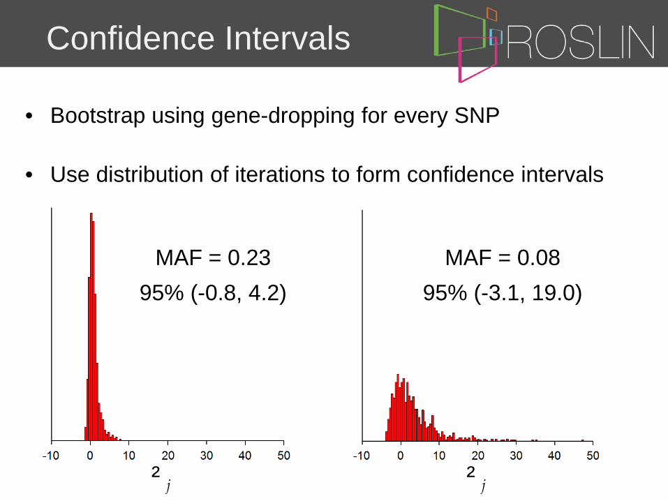
Confidence Intervals
• Bootstrap using gene-dropping for every SNP
• Use distribution of iterations to form confidence intervals
² j
MAF = 0.23
95% (-0.8, 4.2)
MAF = 0.08
95% (-3.1, 19.0)
² j

Results

Line A, SSC07
Position, Mb
² j

Line A, SSC07
95% Confidence Interval
² j
Position, Mb

Line A, SSC07
Significant at 5% level
190 / 2,573 =
7.4%
Position, Mb
² j

Putative QTL, SSC07
animalgenome.org
Average Daily Gain
Position, Mb

Line Comparison, SSC06
Line A Line B
² j
Position, Mb

Significant at 5% level
² j
Line A Line B
Position, Mb

Changes in Heterozygosity Line A Line B
Confidence Intervals 1% 5% Upper
0.5% Upper 2.5%
Lower 0.5%
Lower 2.5%
Whole Genome 0.86% 4.05% 0.33% 1.59% 0.53% 2.46%
SSC01
SSC02
SSC03
SSC04
SSC05
SSC06
SSC07 7.4% SSC08
SSC09
SSC10
SSC11
SSC12
SSC13
SSC14
SSC15
SSC16
SSC17
SSC18
Confidence Intervals 1% 5% Upper
0.5% Upper 2.5%
Lower 0.5%
Lower 2.5%
Whole Genome 1.70% 6.14% 0.65% 2.66% 1.05% 3.48%
SSC01
SSC02
SSC03
SSC04
SSC05
SSC06
SSC07
SSC08
SSC09
SSC10
SSC11
SSC12
SSC13
SSC14
SSC15
SSC16
SSC17
SSC18
= Evidence for excessive change in heterozygosity

Summation

• With high density data we can:
1. Identify regional variations in selection
2. Examine level of conformity with pedigree model
Aims

Conclusions
• Evidence of diversity loss at specific regions
Putative QTL identification (Line A, SSC07)
• Varying impact between lines (SSC06)
Trait Architecture
Power
Future - Haplotyping

• With high density data we can:
1. Identify regional variations in selection
2. Examine level of conformity with pedigree model
Aims

Implications
• Evidence for inadequacy of pedigree model (Line B)
• Genomic Optimal Contributions
• Precision inbreeding at SNP level
• ‘ ‘ Regional loss of diversity, provided maintained elsewhere

Acknowledgements
John Woolliams Ricardo Pong-Wong
Pieter Knap Valentin Kremer Dave McLaren Olwen Southwood Nan Yu