the impact of behavioral and economic drivers on gig
TRANSCRIPT

The Impact of Behavioral and Economic Driverson Gig Economy Workers
Gad AllonThe Wharton School, University of Pennsylvania, [email protected]
Maxime C. CohenDesautels Faculty of Management, McGill University, Montreal, Canada, [email protected]
Wichinpong Park SinchaisriThe Wharton School, University of Pennsylvania, [email protected]
Problem Definition: Gig economy companies benefit from labor flexibility by hiring independent workers
in response to real-time demand. However, workers’ flexibility in their work schedule poses a great challenge
in terms of planning and committing to a service capacity. Understanding what motivates gig economy
workers is thus of great importance. In collaboration with a ride-hailing platform, we study how on-demand
workers make labor decisions; specifically, when to work and for how long.
Academic/Practical Relevance: Our model offers a way to reconcile competing theories of labor sup-
ply regarding the impact of financial incentives and behavioral motives on labor decisions. We are interested
in both improving how to predict the behavior of gig economy workers and understanding how to design
better incentives.
Methodology: Using a large comprehensive dataset, we develop an econometric model to analyze work-
ers’ labor decisions and responses to incentives while accounting for sample selection and endogeneity.
Results: We find that financial incentives have a significant positive influence on the decision to work and
on the work duration—confirming the positive income elasticity posited by the standard income effect. We
also find support for a behavioral theory as workers exhibit income-targeting behavior (working less when
reaching an income goal) and inertia (working more after working for a longer period).
Managerial Implications: We demonstrate via numerical experiments that incentive optimization based
on our insights can increase service capacity by 22% without incurring additional cost, or maintain the same
capacity at a 30% lower cost. Ignoring behavioral factors could lead to understaffing by 10–17% below the
optimal capacity level. Lastly, inertia could be a potential sign of workers’ loyalty to the platform.
Keywords : empirical operations, behavioral operations, gig economy, incentives, sample selection, inertia
1. Introduction
Gig economy is a labor-sharing market system where workers engage in short-term projects or
freelance work as opposed to permanent jobs. In 2019, 57 million Americans or 35% of the U.S.
workforce engaged in gig work (Intelligence 2019), providing a wide range of services, from ride-
hailing (e.g., Uber, Lyft) to food delivery (e.g., DoorDash, Caviar) to web development (e.g.,
Upwork, Fiverr). The size of the independent workforce is growing three times faster than the overall
1

2 Allon, Cohen, and Sinchaisri: The Impact of Behavioral and Economic Drivers on Gig Workers
U.S. workforce growth since 2014 and it is estimated that by 2025, the majority of the workforce
will participate in the gig economy—leading to a global GDP boost of $2.7 trillion (Manyika
et al. 2015). The unique and novel feature of this system relates to the nature of employment:
independent workers can freely choose their work schedule as well as seamlessly switch between
multiple platforms to provide service. Such flexibility attracts many workers to the gig economy.
Companies also greatly benefit from increased labor flexibility as they can hire workers with
different skill levels to work at different times while compensating them for the work they perform.
Like any other market, the key to success in the gig economy lies in the effective matching of supply
with demand. Firms need to ensure that their services appeal not only to customers (demand) but
also to independent service providers (supply). This poses an enormous challenge in planning and
committing to a service capacity both during peak hours when demand is high and during off-peak
times when only a handful of workers are needed. Policymakers have also joined the conversation,
concerned with how such work structures might affect workers. For instance, New York City passed
fatigued driving prevention rules as part of its Vision Zero initiative in 2017, limiting the number
of daily and weekly hours a ride-hailing driver can work with the goal of reducing driver fatigue
and enhancing road safety. In 2019, the European Parliament approved new rules that provide
minimum rights and enforce better job transparency and compensation for gig workers.
To examine how firms can staff the right number of on-demand workers at the right time and
how policymakers can develop effective regulations, it is important to first understand how gig
workers make labor decisions. For decades, economists have studied how labor supply is influenced
by economic incentives and behavioral motives. The standard income effect predicts that workers,
as lifetime-utility maximizers, are more likely to work or supply more labor in response to a higher
wage. While several observational studies find evidence for this theory (e.g., Oettinger 1999, Sheldon
2016), other studies suggest the opposite prediction. NYC taxi drivers are found to work for fewer
hours on a high-paying day and more likely to quit working in response to higher accumulated
income due to reference-dependent behavior with respect to earnings (e.g., Camerer et al. 1997,
Thakral and To 2019). In other words, their decisions are based on reaching a target level of income
or income target. Providing further support for the behavioral theory of labor supply, Crawford
and Meng (2011) and Farber (2015) suggest that workers’ behavior could perhaps be influenced
by a target level of work duration or time target.
Our paper aims, in part, to reconcile this ongoing debate by proposing a framework to explain
labor decisions through both economic incentives and behavioral motivations. Recent work in
operations management in the context of the gig economy has focused on the system equilibrium or
on social welfare (e.g., Cachon et al. 2017, Taylor 2018). To our knowledge, among the papers that
focus on the supply side (e.g., Benjaafar et al. 2019, Dong and Ibrahim 2020), our work is the first
Allon, Cohen, and Sinchaisri: The Impact of Behavioral and Economic Drivers on Gig Workers 3
to empirically examine the causal effect of behavioral and economic factors on gig economy workers’
decisions and to incorporate their behavior into the optimization of financial incentives. Our work
also follows calls for advancing behavioral operations research by studying worker behavior in new
work environments such as on-demand services and freelancing platforms (Donohue et al. 2020,
Chen et al. 2020).
Research questions and methodology. Our key research questions are: (i) How do gig econ-
omy workers make labor decisions? How do they react to incentives? What are the factors that
shape their work schedule decisions? Are their decisions rational or do they exhibit behavioral
biases? and (ii) How can gig companies set incentives to effectively recruit workers? How can they
meet the desired service level by taking into account workers’ behavior and offering them the right
incentives?
We answer these questions by estimating an econometric model of workers’ labor decisions and
conducting numerical experiments on incentive optimization. Prior empirical studies on the rela-
tionship between wage and labor decisions have not distinguished between the decision of whether
to work and the work duration decision and instead treated them essentially as a single decision due
to data limitations. Through our collaboration with a U.S. ride-hailing company, we overcome this
challenge by leveraging our rich dataset which contains real-time information on financial incentives
regardless of drivers’ subsequent labor decisions. Accordingly, we gain a clearer insight into drivers’
decisions to work by investigating drivers who chose not to work during a particular period. In our
empirical model, we address econometric challenges such as sample selection and omitted variable
biases and we account for drivers’ heterogeneity and real-time market conditions and competition.
Finally, we propose an optimization heuristic for incentives and conduct counterfactual simulations
to examine its performance and quantify potential losses if the company ignores workers’ behavior
when designing incentives.
Contributions. Our paper contributes to the economics and operations literatures in four ways.
First, we offer a potential way to reconcile the two competing theories of labor supply by showing
that workers respond to wage variation in the same way as suggested by the standard income effect,
while also exhibiting reference-dependent behavior with respect to accumulated earnings. We find
that an hourly wage has a positive impact on both the decision to work and on the work duration.
However, our proxy for unobserved income targets—accumulated earnings from earlier hours of
the same day or earlier days of the week—has a negative impact on both decisions. This finding
provides support for an income-targeting behavior; that is, workers work less as they are closer
to their income goal. Second, we unravel a new behavioral driver of labor decisions, inertia. Our
results indicate that workers’ recent work duration (from earlier hours of the same day or earlier

4 Allon, Cohen, and Sinchaisri: The Impact of Behavioral and Economic Drivers on Gig Workers
days of the same week) has a consistent and positive influence on the decision to continue working
and on subsequent work duration. This phenomenon appears to capture the tendency of workers
to make the same work decision as their recent ones or inertia. Furthermore, it can potentially hint
at workers’ loyalty to the focal platform. Third, we demonstrate that behavioral factors play an
important role in workers’ labor decisions. Both in-sample and out-of-sample analyses suggest that
workers’ reaction to accumulated earnings and past work duration are key drivers of their labor
decisions. We then demonstrate via simulations that not accounting for these behavioral factors
would result in understaffing by 10–17%. Finally, we apply our insights to prescribe operational
decisions and conduct regulatory impact analysis. Specifically, we show that if the company opti-
mizes their incentive policy accounting for workers’ behavior, it can increase the capacity by 22%
without incurring additional cost or maintain the same service level at a 30% lower cost.
2. Labor Supply Theories and Hypotheses Development
Economists have offered two different perspectives centered around the elasticity of labor supply.
On the one hand, the traditional approach follows a lifecycle model where individuals maximize
their lifetime utility and predicts that workers exhibit positive income elasticity. On the other hand,
empirical studies, notably in the context of taxi drivers, suggest that income elasticity could be
negative if workers are loss averse and benchmark their earnings relative to a reference point. It is
unclear whether existing findings can apply to gig economy workers who have full discretion over
their work schedule. In this section, we review in greater detail the two contrasting models of labor
supply and develop hypotheses for the behavior of gig economy workers.
2.1. Traditional Model of Labor Supply
In the neoclassical microeconomics tradition, each worker is a rational agent who maximizes lifetime
utility. A positive wage shock should then lead to a larger group of workers joining the force or to
a higher level of activity from workers. In other words, workers are expected to exhibit a positive
wage elasticity (e.g., work more when facing a wage increase). This perspective seems plausible but
finding evidence in the field has been challenging as in reality workers cannot easily adjust their
work hours. However, positive elasticities have been observed among workers who have some level
of discretion over their schedule, such as pipeline workers (Carrington 1996), vendors in a baseball
stadium (Oettinger 1999) and fishermen (Stafford 2015). These studies find that wage shocks,
typically driven by temporary demand variation, have a positive effect on labor supply—both on
the number of workers and work hours.
2.2. Behavioral Model of Labor Supply
The seminal work by Camerer et al. (1997) studies NYC taxi drivers and finds substantial negative
elasticities, suggesting that drivers’ daily decisions on work hours are influenced by their individual

Allon, Cohen, and Sinchaisri: The Impact of Behavioral and Economic Drivers on Gig Workers 5
income targets (known as the income-targeting effect). Using data from a different set of NYC
taxi drivers, Farber (2005) and Farber (2008) find that the probability to stop working is closely
related to the realized income earned in the same day and it increases once the income target is
reached, but conclude that the findings are not robust. Crawford and Meng (2011) implements
similar econometric strategies to estimate models based on the reference-dependent preferences
theory, which allows for consumption and gain-loss utilities. The authors conceptualize drivers’
targeted levels of income and work hours and find that stopping probabilities are more influenced
by the second target they reach on a given day. More recently, Thakral and To (2019) estimates
a structural model of labor supply of NYC taxi drivers, allowing a time-dependent relationship
between earnings and the stopping probability. Their results confirm that the income-targeting
effect exists when controlling for the number of work hours. These findings offer a realistic behav-
ioral explanation and align well with insights from behavioral economics; however, support for the
behavioral theory has been lacking outside the taxi industry.
2.3. Labor Supply in the Gig Economy
The gig economy offers workers a flexible work schedule. As gig work appeals to a broad range
of workers with different backgrounds and preferences, predicting the worker turnout or service
capacity at any point in time is remarkably challenging. A common way to incentivize workers to
join and to keep active workers engaged is to offer dynamic financial incentives. Real-time bonuses,
such as Uber’s surge prices and Caviar’s Peak Pay, reward workers who work during busy periods
with high demand. Beyond direct monetary rewards, several companies employ a combination of
gamification and psychology and offer non-monetary incentive programs. For example, Uber drivers
can earn badges for achievements, from excellent service to entertaining ride, and are constantly
reminded of how close they are to their earning goals. While these incentive strategies are prevalent
in practice, less is known in academic research about their influence on workers’ labor decisions.
Our paper belongs to the fast-growing research trend that examines operational and pricing
decisions in the context of the gig economy (for a review, see Benjaafar and Hu 2020). Most
relevant to our work are studies that examine how dynamic wages affect supply and consider the
problem of designing the optimal incentives to coordinate supply with demand for on-demand
service platforms. Dynamic wages due to surge pricing have been shown to entice ride-hailing drivers
to work longer (Chen and Sheldon 2016) and benefit drivers via better utilization (Cachon et al.
2017). Hu and Zhou (2019) studies the contracts under which the platform takes a fixed cut from
workers’ earnings and demonstrates good performance among flat-commission contracts. Taylor
(2018) shows that the uncertainty in workers’ opportunity costs or in delay-sensitive customers’
valuations can lead the intermediary to raise the price during congestion. Our work focuses on

6 Allon, Cohen, and Sinchaisri: The Impact of Behavioral and Economic Drivers on Gig Workers
the supply side behavior and the need to use incentives to motivate flexible workers. There are
relatively few studies that investigate worker behavior and its impact on the platform’s operational
decision. Most of these studies are of theoretical nature and focus on the equilibrium of matching
supply with demand (see, e.g., Ibrahim 2018, Benjaafar et al. 2019, Dong and Ibrahim 2020).
The only empirical studies that incorporate worker behavior in a gig economy setting to our
knowledge are Sheldon (2016), Karacaoglu et al. (2018), and Chen et al. (2019). Sheldon (2016) finds
that Uber drivers’ income elasticities are significantly positive and increasing over time, suggesting
that if income targeting does exist, it would only be temporary and moderated by experience.
Karacaoglu et al. (2018) studies e-hailing taxi drivers in South America and finds that drivers’
response to real-time information about other drivers ’ locations could explain different utilization
they can achieve. Chen et al. (2019) documents how Uber drivers value real-time flexibility and
estimates the driver surplus from having a flexible schedule. The authors find that drivers earn
higher surplus from Uber’s flexible model relative to less flexible arrangements. While these papers
rigorously capture how gig workers respond to incentives and information, their models do not
consider potential behavioral factors in explaining workers behavior. This is due to data limitations
given that most datasets record only the trips that happened. In our dataset, however, we observe
the information available to drivers even when they decided not to work. We focus on the behavior
of gig workers and on how the platform can improve its operational decisions by understanding
such behavior.
2.4. Hypotheses Development
We are interested in studying how gig economy workers make labor decisions, specifically whether
they will work at a particular time and, if so, for how long. Labor decisions typically depend on
multiple factors such as weather and external commitments. Yet, these are not controlled by the
platform and, thus, while we attempt to control for such factors, we focus on the impact of economic
drivers (hourly wage) and behavioral factors (workers’ income and time targets). Several companies
have exploited workers’ tendency to set goals by helping workers track their progress toward the
goals and nudging them to work for longer. Since individuals’ targets cannot be observed, we use
workers’ accumulated earnings since the beginning of their work day as a proxy for their income
target and the duration of their work so far as a proxy for their time target. We next present our
hypotheses regarding the impact of each factor on gig economy workers’ labor decisions.
H1: A higher wage increases the probability of working and the work duration.
Following the standard income effect (see §2.1), we expect that a higher hourly wage will increase
the probability of working. Empirical studies of workers who have discretion over their work hours
suggest that workers adjust labor decisions in the same direction as wage (see, e.g., Oettinger

Allon, Cohen, and Sinchaisri: The Impact of Behavioral and Economic Drivers on Gig Workers 7
1999, Stafford 2015). We posit that gig workers also exhibit a positive income elasticity as they
have full control over their schedule. Unlike traditional employment, gig work tends to be smaller
and temporary projects (e.g., assembling furniture, driving within a city) that require less time to
complete. Consequently, work decisions are made more frequently and for a shorter time frame.
The objective is therefore likely to maximize utility (e.g., earnings) in the following period. We
still believe that there exists a behavioral explanation of labor supply, but such effect would be
driven by accumulated earnings or work hours instead (see H2 and H3 below). Past studies that
provide support for an income targeting effect only modeled the relationship between the number
of work hours and the average daily wage. We postulate that the negative impact on work duration
will only be apparent during specific times of day (days of week), when workers might be closer to
reaching their daily (weekly) income targets. Thus, when controlling for both accumulated income
and work hours separately, we should observe a positive income elasticity.
H2: Higher accumulated earnings decreases the probability of working and the work
duration. Studies of taxi drivers including Camerer et al. (1997), Farber (2008), and Thakral
and To (2019) provide support for an income-targeting behavior; that is, the probability to stop
working increases once the income target is reached. Thakral and To (2019) further demonstrates
that drivers’ decisions are highly influenced by recent earnings. Gig workers are also likely to
be influenced by the income-targeting effect, as tracking their progress towards the income goal
is much easier. Several gig platforms provide real-time information about workers’ recent work
activities and earnings through their apps and also provide frequent feedback about their earnings
(e.g., after every completed trip for ride-hailing drivers). An alternative explanation of the negative
impact of accumulated income is related to fatigue. Specifically, higher accumulated earnings could
indicate a greater level of effort. Consequently, workers who experienced more fatigue would work
for a shorter time. As a result, we expect to see a negative impact of the accumulated earnings on
both the probability of working and on the work duration.
H3: Longer time worked decreases the probability of working and the work duration.
Previous work in labor economics suggests another type of targeting behavior: time targeting.
Crawford and Meng (2011) develops a structural stopping estimation model that allows for reference
points in both daily income and work duration among taxi drivers and concludes that drivers are
loss averse relative to both reference points. Agarwal et al. (2015) and Farber (2015) find that the
probability of ending a work shift is positively related to cumulative work hours. As discussed in H2,
fatigue could also be explained by work duration. Recent findings suggest that work performance
deteriorates toward the end of long shifts among paramedics (Brachet et al. 2012) and part-time
call center agents (Collewet and Sauermann 2017). Thus, we expect that the longer the workers
have recently worked, the less likely they would continue working and, if they do work, the work
duration would be shorter relative to those with a shorter past work duration.

8 Allon, Cohen, and Sinchaisri: The Impact of Behavioral and Economic Drivers on Gig Workers
3. Data: Ride-hailing Platform in New York City
To answer our research questions, we collaborate with an on-demand ride-hailing company (referred
to as “the company” or “the platform”) and analyze a large comprehensive dataset of driving
activities and financial incentives in NYC over a period of 358 days (from October 2016 to Septem-
ber 2017). Our data includes: each driver’s vehicle type, experience with the platform, number of
hours driven, and financial incentives offered and earned. The key advantage of our data is that
we observe the incentives that were offered to every driver regardless of the decision to drive. In
other words, even for drivers who decided not to drive for a particular time period, we still know
their offered wage and promotions for that period. In total, we have several million driver-shift
observations and several thousand unique drivers.1 We next present an overview of the platform
and report descriptive statistics of working shifts, financial incentives, and vehicle types.
3.1. Platform Overview
The company is a ride-hailing online platform that offers services in many cities worldwide. The
users (riders) may request rides in real-time through a smartphone app. Then, the platform will
match riders with available drivers. This platform offers a shared service (i.e., several passengers
heading in the same direction may share the same vehicle). To make the service more efficient,
passengers can be picked up and dropped off at an optimized location near the exact requested
locations. Finally, the vast majority of drivers are compensated according to a guaranteed hourly
rate regardless of the number of completed rides. We focus on drivers who are paid by the hour
as this scheme resembles the traditional wage model but with more flexibility on the drivers’ side.
This allows us to investigate how drivers’ work decisions are influenced by variations in monetary
incentives.
Figure 1 Breakdown of shifts for each operating day
3.2. Shifts and Work Schedule
Each operating day is divided into six shifts specified by the company (see an illustration in
Figure 1): morning non-rush hours from midnight to 7am (AM Off-peak), morning rush hours from
7 to 9am (AM Peak), midday from 9am to 5pm (Midday), afternoon rush hours from 5 to 8pm
(PM Peak), evening non-rush hours from 8 to 9pm (PM Off-peak), and late night from 9pm to
midnight (Late night). The largest volume of activities happen during PM Off-peak, followed by
1 We cannot reveal the exact number of drivers and the size of our dataset due to confidentiality. However, theseexact numbers do not affect any of our results or findings.

Allon, Cohen, and Sinchaisri: The Impact of Behavioral and Economic Drivers on Gig Workers 9
PM Peak, and Midday, while AM Off-peak hours are the least busy. In our data, an average driver
works 2.1 days per week and 6.35 hours per day.
In this paper, we analyze drivers’ behavior at both the shift and day levels. We control for the
day of the week to account for demand and supply variation. In our data, 49.46% of all completed
trips occurred between Tuesday and Thursday, potentially confirming the popularity of the service
among city commuters. Monday and Friday trips account for 30.91% of all trips, while weekend
trips account for 19.62%. While drivers are allowed to flexibly decide their own work schedules,
they often stick to their “regular” times. For example, 30.41% of drivers never worked on weekends.
91.07% of drivers’ working days did not overlap with midnight (e.g., they did not work overnight).
3.3. Earnings and Incentives
Drivers receive a shift-specific hourly rate for the duration they are active on the platform. They
are considered active when they log on to the driver application on their mobile device and report
to their designated start location. This compensation scheme can be considered as a guaranteed
payment, in contrast to a commission-based contract that compensates drivers for each completed
trip, which is commonly used by several platforms. It is possible under this scheme that drivers
could be paid even if there are no ride requests for the entire hour.2 Similar schemes are used by
other gig platforms such as DoorDash, GoPuff, and HourlyBee.
The guaranteed hourly offer comprises two components: a base rate and a promotional rate.
These two rates vary over time (shifts and days of week) and across different drivers. The base rate
for each driver is decided when the driver joins the platform for the first time. For the same driver,
the base rate may be different across shifts and across days of the week, but typically remains
the same across weeks. In addition to the base rate, drivers are frequently offered promotional
incentives. Rate-based promotions provide a multiplicative bonus to the hourly base rate during
specific times (e.g., during 2× shifts, drivers earn twice the base rate). 32.71% of shifts in the data
include rate-based promotions and the average promotion rate is an additional 50.36% of the base
rate or approximately 1.5×.
At the time of our data, incentives were decided as follows: First, the platform sets a number
of promotional rates as benchmarks. Then, an algorithm uses these rates to assign the final rate
for each driver based on recent work history and vehicle type. Both the base and promotional
rates are specific to each driver. The platform then sends text messages to drivers every evening
to communicate the rates for the following day. This suggests that drivers are likely to plan their
work schedule ahead of time and there is no internal competition for better rates among drivers.
2 To ensure that drivers are not working for other platforms at the same time, the app will redirect idle drivers to anew waiting location every few minutes. Drivers have to confirm they reach the location via GPS.

10 Allon, Cohen, and Sinchaisri: The Impact of Behavioral and Economic Drivers on Gig Workers
Occasionally, drivers may receive real-time adjustments to their rates but will never experience
lower rates than initially informed. All rates are pro-rated to the actual amount of time worked in
a given shift. Earnings are cumulative until the end of the week when drivers have the option to
transfer their eranings to their bank account.
3.4. Drivers and Vehicle Types
Drivers are identified by a unique ID. For each shift, we observe the decision to work (i.e., to
become active) for every driver registered in the system. For drivers who started working after the
first day of our dataset, we record both their first day joining the platform and their first work
day to control for their experience with the platform. Similarly, we observe the last day of being
registered with the platform for some drivers if they left within the duration of our data. These
allow us to control for drivers’ experience, tenure, and span of their service for the focal platform.
For the analysis conducted in this paper, we only consider the drivers who own a single vehicle
(89.9% of all drivers). There are six types of vehicles: a 3-passenger sedan, a small 3-passenger
SUV, a medium 4-passenger SUV, a large 5-passenger SUV, a 5-passenger van, and a 6-passenger
van. We exclude van drivers from our analysis as the majority of them lease their vehicle from the
company rather than owning their vehicle or leasing it from an external third party, leaving us with
86.3% of the original pool of drivers. For our main analysis, we present the results for two types of
vehicles: sedan and large SUV, which are 33.2% of the pool. We make an assumption that drivers
of different vehicle types may have fundamentally different utilities and preferences. Sedan vehicles
are generally less expensive to maintain than SUVs, while SUV drivers may have a different set of
outside opportunities (e.g., qualified for both regular and XL services). From our data, we observe
that SUV drivers typically work more frequently and for longer hours relative to sedan drivers. We
obtain similar qualitative results for other vehicle types; but omit them for conciseness.
3.5. Supplementary Data: TLC Trip Records
We incorporate trip records for other similar services in the same region to capture the real-time
market conditions. Information about taxi and for-hire vehicle (FHV) trips in New York City have
been collected by the Taxi and Limousine Commission (TLC) and publicly released since 2009.3
In particular, we analyze 101,487,565 yellow taxi trips and 129,868,077 FHV trips operated by
four major service providers (including our focal platform) in the city between October 2016 and
September 2017 (i.e., the duration of our data). Taxi trip records include date, time, and location
(at the neighborhood level) of every pick-up and drop-off, itemized fares, and driver-reported
passenger counts. FHV trip records prior to July 2017 consist of date, time, and location of each
pick-up and the dispatching base associated with a ride-hailing platform. Starting from July 2017,
3 https://www1.nyc.gov/site/tlc/about/tlc-trip-record-data.page

Allon, Cohen, and Sinchaisri: The Impact of Behavioral and Economic Drivers on Gig Workers 11
we also observe date, time, and location of each drop-off by FHV drivers. In §4.1, we discuss the
metrics that we construct to control for market conditions and competition intensity.
4. Empirical Approach
To test the hypotheses developed in §2, we estimate the impact of financial incentives, income and
time targets, and other covariates on two labor decisions: (i) whether to work or not and (ii) work
duration. We assume that drivers make both decisions at the beginning of each shift or day. We
conduct our analyses at two levels, within-day (shift level) and across-days (day level), as well as
for each vehicle type separately. This allows us to understand how variations within the same day
or across days affect drivers’ decisions and to capture vehicle type-specific heterogeneity. Drivers
operating different vehicle types may have different preferences, costs, and utility functions, and
thus make their labor decisions differently. In this section, we first introduce our econometric model
and key covariates, then provide details of our estimation method, and finally discuss the empirical
challenges and our strategies to address them.
4.1. Empirical Model and Estimation Details
As discussed, our dataset provides a unique advantage as we observe the financial incentives offered
to every driver for every shift as long as the driver already joined the platform and have not yet
terminated their drivership. This allows us to study two stages of labor decisions and control for
potential sample selection bias (see §4.2.1 for further discussion). Our approach therefore adapts
the two-stage Heckman estimation method (Heckman 1979) to first estimate the decision to work
across all drivers using a probit regression, and then estimate the work duration for drivers who
chose to work for any given shift or day using an OLS regression.
4.1.1. Outcome variables. The decision of the first stage is captured by the binary variable
Drivei,t. Specifically, Drivei,t = 1 if driver i works during shift (or day) t and Drivei,t = 0 oth-
erwise. In the second stage, conditional on working during shift (or day) t, Hoursi,t represents
work duration in hours for driver i during t. Given the long tails in Hoursi,t, we apply a Box-Cox
transformation conditional on the covariates to normalize its distribution and homogenize its vari-
ance. Our results are robust under other types of transformation (e.g., logarithm, square root) and
also without a transformation. We exclude outliers defined as drivers whose work duration during
a given shift or day exceeds the 1.5 interquartile ranges (IQRs) or less than 5 minutes. We also
exclude public holidays from our analysis.
4.1.2. Key covariates. We focus our analysis on three key drivers of labor decisions. (i)
Financial incentives. We use the hourly offer rate (i.e., the sum of hourly base rate and promotions,
if available), denoted as wi,t for driver i during shift (or day) t, for the first stage. Similarly,

12 Allon, Cohen, and Sinchaisri: The Impact of Behavioral and Economic Drivers on Gig Workers
conditional on working, the second stage’s financial incentives are taken from the hourly earnings
rate (i.e., the sum of hourly base rate and promotions, if available), denoted as wi,t. (ii) Income
targets. As we do not directly observe drivers’ income targets, we use cumulative earnings since the
beginning of the day (week) until the focal decision point as a proxy for a daily (weekly) income
target. We refer to this covariate as income so far or ISF . The rationale behind this proxy is that,
as the driver starts accumulating earnings, the higher ISF , the closer they are to their privately
known targets. The same proxy is used in the literature (e.g., Crawford and Meng 2011, Thakral
and To 2019). (iii) Time targets. Similarly, we use cumulative work hours since the beginning of
the day (week) until the focal decision point as a proxy for a daily (weekly) time target. We refer
to this covariate as hours so far or HSF . Given our observation that over 90% of the data do not
include overnight work, we assume that daily targets and progress are “reset” at midnight (e.g.,
the driver starts working toward a new target for the new day). Similarly, as the majority of work
occurred during weekdays, we assume that weekly targets are reset at the end of every Sunday.
Our results are robust to different constructs of targets and flexible frequency of target reset.
4.1.3. Two-stage estimation. Let wi,t, wi,t, ISFi,t, and HSFi,t be hourly offer, hourly earn-
ings rate, cumulative income, and cumulative work hours of driver i at the beginning of time t,
respectively. The variables Xi,tXi,tXi,t and Zi,tZi,tZi,t are other relevant covariates that affect the decision to
work and work duration, respectively. We model the two stages of labor decisions, Drivei,t and
Hoursi,t, of driver i at time t as follows.
Houri,t =
{Hour∗i,t if Drivei,t = 1
unobserved otherwise(1)
Drivei,t =
{1 if Drive∗i,t > 0
0 otherwise(2)
Drive∗i,t = α0,i +αwwi,t +αISF ISFi,t +αHSFHSFi,t +αXi,tαXi,tαXi,t + vi,t (3)
Hour∗i,t = β0,i +βwwi,t +βISF ISFi,t +βHSFHSFi,t +βZi,tβZi,tβZi,t +ui,t (4)[σ2v
σ2u
]∼N
([00
],
[1 ρσu
ρσu σ2u
]). (5)
The two stages that we estimate are given by:
P (Drivei,t = 1|Xi,tXi,tXi,t) = Φ(α0,i +αwwi,t +αISF ISFi,t +αHSFHSFi,t +αXi,tαXi,tαXi,t), (6)
f(Houri,t) = β0,i +βwwi,t +βISF ISFi,t +βHSFHSFi,t +βZi,tβZi,tβZi,t + θλi,t +ui,t, (7)
where Φ(·) is the normal c.d.f. and λi,t is the inverse Mills ratio (IMR) calculated from the predicted
probability in Equation (6) (“Choice Equation”). Thus, we essentially estimate a probit model for
the work decision in Equation (6) and compute the IMR for each observation. We then fit an OLS
Allon, Cohen, and Sinchaisri: The Impact of Behavioral and Economic Drivers on Gig Workers 13
model of the (transformed) work duration conditional on all covariates and the IMR (Equation (7)),
while controlling for the drivers who worked (“Level Equation”). The estimated coefficient θ= ρσu
will potentially confirm the existence of a sample selection bias. We next discuss in detail the
estimation methodology for each stage.
Choice: Control function probit. The first stage is based on a probit model of labor decisions,
Drivei,t. We address a potential endogeneity related to financial incentives and past work decisions
by taking an instrumental variable (IV) approach (see §4.2.2). A commonly used two-stage least
squares (2SLS) can provide inconsistent estimates for a probit model as certain properties of the
expectation and linear projection operators do not carry over to nonlinear models (Newey 1987).
Instead, we implement the control function method to account for endogeneity for our nonlinear
probability model (Imbens and Wooldridge 2007, Wooldridge 2015). The first step is identical to
the first step of 2SLS, that is, we estimate an OLS regression of the endogenous variable (wi,t)
on exogenous covariates and instrumental variables. We can then keep the endogenous variable in
the model and include the residuals from the previous regression as an additional regressor. The
intuition behind this method relies on using the instrument to split the unmeasured confounders
into two parts, one that is correlated with the endogenous regressor and one that is not. We
correct for the standard errors using the standard deviation of the residuals following Imbens and
Wooldridge (2007).
We also allow for drivers and time fixed effects throughout our estimation. Adding fixed effects
to the nonlinear choice equation is known to generate the incidental parameters problem. More
precisely, the usual asymptotic properties of the maximum likelihood estimator are not guaranteed,
thus leading to a biased and inconsistent estimator (Greene 2004). Fortunately, recent developments
in bias correction, such as the jackknife estimation method (see Hahn and Newey 2004, Dhaene
and Jochmans 2015 for more details on this method), allow us to obtain asymptotically unbiased
estimates and alleviate the incidental parameters problem. The final step for this stage is to compute
the IMR for each observation using the fitted probability.
Level: Fixed effects 2SLS. The second stage aims to estimate the work duration, Houri,t, condi-
tional on the driver working during the focal time period. The hourly earnings rate, wi,t, is likely
to be endogenous. Incorporating the IV approach to the level equation is straightforward, as we
can simply perform a 2SLS regression in which we first obtain the predicted value of wi,t based
on exogenous covariates and the IVs. We transform the observed work duration using a Box-Cox
approach conditional on all covariates to alleviate heteroskedasticity. Finally, as we include the
IMR as one of the regressors in the second stage, we bootstrap the standard errors by repeating
our analysis on resampled datasets.

14 Allon, Cohen, and Sinchaisri: The Impact of Behavioral and Economic Drivers on Gig Workers
Other covariates. To capture drivers’ heterogeneity, we first include a driver-specific intercept in
both stages even if we already perform separate analyses for drivers with different vehicle types. We
also include other time-varying driver-specific covariates that could reflect their work habits. Short-
term habits are captured by historical work duration on the same day and shift of the previous
week and the total hours worked during the previous week. Long-term habits are captured by the
driver’s experience (i.e., whether they are new to the platform and their tenure) and also through
drivers’ fixed effects. Month and day-of-week fixed effects are also included to capture seasonal
trends. The sets of regressors in our main model are:
• Choice: hourly offer (w), cumulative earnings (ISF ), cumulative work hours (HSF ), number
of hours worked last week, new driver indicator, humidity, apparent temperature, precipitation
probability, number of other ride-hailing trips in the previous shift or day (in thousands).
• Level: hourly earning rate (w), cumulative earnings (ISF ), cumulative work hours (HSF ),
number of hours worked on the same shift of last week, humidity, apparent temperature,
precipitation probability, number of other ride-hailing trips during the same shift or day (in
thousands).
4.2. Empirical Challenges and Strategies
4.2.1. Sample selection bias. Previous studies such as Camerer et al. (1997) and Sheldon
(2016) investigated the relationship between the number of work hours and the hourly wage con-
ditional on drivers who worked on a given day. This would not be a concern if drivers randomly
decide whether to work or not. In reality, however, it is more plausible that they make such deci-
sions based on factors which are not observed by the researcher. In other words, the selection of
drivers who choose to work at a given time is not random. Consequently, this approach may yield a
biased estimate of the sensitivity to incentives (i.e., income elasticity). Fortunately, the comprehen-
siveness of our data offers an opportunity to address this challenge. Since we observe incentives for
all drivers on every shift regardless of their work decisions, we can directly estimate the selection
problem. As presented in §4.1.3, we employ a modified two-stage Heckman estimation method for
our analysis.
While Heckman-type selection model has been widely used in several applications, it has also
been criticized on its potential pitfalls, particularly the weak nonlinearity of the IMR and the
multicollinearity of regressors in both stages (Puhani 2000). To address these concerns, we carefully
choose the sets of regressors for both stages (Xi,tXi,tXi,t and Zi,tZi,tZi,t) to be different (as shown in §4.1.3) and
we check for collinearity by regressing the IMR on the regressors of the second stage. On average,
the standard deviation of the errors is 44.52% less than the standard deviation of the IMR, which
suggests a substantial difference. We also consider an alternative approach suggested by Puhani
(2000): estimating a subsample OLS or a two-part model. In the two-part model, a binary choice

Allon, Cohen, and Sinchaisri: The Impact of Behavioral and Economic Drivers on Gig Workers 15
model is estimated for the probability of observing a positive-versus-zero outcome (e.g., the number
of work hours). This is essentially the same as the first stage of our main approach. Conditional
on a positive outcome (e.g., drivers who worked during a particular shift or day), a separate OLS
regression model is estimated for the work duration (Cragg 1971, Madden 2008, Farewell et al.
2017). This is the same as the second stage of our main approach excluding the IMR. We report
the estimates from both the two-part model and our main approach in §5. Finally, as a robustness
check, we consider the Dahl’s approach by using a basis spline to approximate the choice probability
(Dahl 2002). For more details on the approach, we refer the reader to Bourguignon et al. (2007)
that provides Monte Carlo comparisons across different selection models and to Bray et al. (2019)
that implements this correction to model proximity-based supplier selection. In our context, the
choice for each driver is binary. Our results remain consistent and are presented in Appendix B.1.
4.2.2. Endogeneity. As discussed in §2.1, the standard income effect suggests that financial
incentives encourage workers by increasing their likelihood of working or work duration. Neverthe-
less, quantifying the effect of incentives by regressing the labor decision on financial incentives can
lead to misleading results. In our dataset, we observe that a smaller fraction of drivers who received
an hourly offer of $65 decided to work relative to those who received $45 per hour. One possible
implication is that financial incentives are not effective in convincing some drivers. Alternatively,
these appealing promotions might have been strategically offered to engage inactive drivers. Con-
sequently, regressing work decisions on financial incentives can lead to an omitted variable bias as
we do not observe the actual algorithm behind these incentives. Overlooking this issue may yield
to a bias estimate of the effect of financial incentives. A common solution is to use instrumental
variables (IVs) that are highly correlated with financial incentives but affect the work decision only
through the incentives (Levinsohn and Petrin 2003).
Instrumental variables. The main endogenous variables in our data are the hourly financial
incentives, wi,t, and the hourly earnings, wi,j. Our ideal instrument should be highly correlated with
each endogenous variable and affect the dependent variable (the decision to drive or the work hours)
only through the endogenous variable. In other words, we are looking for instruments that are not
correlated with the unobserved variables in the error terms. Our industry partner confirmed that
the financial incentives were endogenously determined with respect to (predicted) supply decisions.
Specifically, the firm sets the incentives based on past work history, level of inactivity, and vehicle
type. Different teams are in charge of determining the offers for different vehicle types. This insight
motivated us to focus on instruments that categorize drivers based on these three factors.
Our instrument is based on the notion of co-workers. For each driver who is available to work
at a particular time (i.e., has not terminated their partnership with the platform), we define their
co-workers as the drivers who meet the following conditions: (i) available to work at the same time,

16 Allon, Cohen, and Sinchaisri: The Impact of Behavioral and Economic Drivers on Gig Workers
(ii) drive a different vehicle type, and (iii) have made the same work decision in the past (i.e.,
worked in the same shift in the previous week or previous month). Work decisions are binary such
as working or not. Assuming that random shocks, vi,t and ui,t, are not correlated across drivers, we
propose to use the average hourly offers received by co-workers for the focal period as an IV. This
IV satisfies the relevance condition: since both the focal driver and their co-workers made the same
work decision in the past, their incentives should be highly correlated as the firm would adjust the
incentives for both groups in the same direction. From the first stage of our IV estimation, the
estimate for the instrument is consistently significant and F -statistics for all models are higher than
the conventional threshold of 10. This IV also satisfies the exclusion restriction: current incentives
for co-workers should not directly influence the focal driver’s work decision because (i) the offers
for different vehicle types are decided independently by different teams within the company, (ii)
the focal driver does not have access to co-workers’ incentives information, and (iii) it is unlikely
that drivers compare the offers across different vehicle types.
To test the robustness of our results, we consider two alternative instruments. First, instead of
matching drivers based on their decision to work at a specific time in the past, we now match
drivers based on their decision not to work : the level of past inactivity. For every day in our data,
we categorize drivers into four groups based on each quartile of the number of consecutive days
they have not been working. We refer to the drivers of a different vehicle type who belong to the
same group as co-skippers. Finally, we also consider the instrument used in previous literature (e.g.,
Sheldon 2016), the average hourly offer rate received by all other drivers during the same shift on
the same day as an instrument for the offer rate. We obtain consistent insights under all three
specifications. Further details are deferred to Appendix B.2.
4.2.3. Multicollinearity. A potential concern of including both HSF and ISF in the same
specification is the multicollinearity issue. Correlations between ISF and HSF in our data range
between 0.667 and 0.928, depending on the time of the day and the vehicle type. This issue does
not significantly affect our results because of three reasons. First, despite a positive correlation,
HSF and ISF are not a direct transformation of each other, hence there is no perfect correlation.
Intuitively, HSF increases linearly with time as it denotes the exact amount of time the driver has
been working, while ISF evolves dynamically as it depends on time-varying financial incentives.
Second, multicollinearity generally makes causal inference difficult as the variance of each estimate
would be inflated, leading to statistical insignificance, but the estimate itself would be unbiased.
Our main results (see §5) show that this is not the case for us as both coefficients for HSF and
ISF are statistically significant in most cases. Third, potential problems from high collinearity can
be largely offset with sufficient power (Mason and Perreault Jr 1991). Our dataset consists of a
large enough number of observations to provide sufficient statistical power even when we separately

Allon, Cohen, and Sinchaisri: The Impact of Behavioral and Economic Drivers on Gig Workers 17
estimate our model by vehicle type, day of the week, and shift of the day. Finally, we consider
several alternative approaches to alleviate the multicollinearity concerns, including considering
models with only ISF or HSF , performing localized regressions by controlling for drivers with
similar ISF or HSF , and converting one of the two variables to be categorical. Our insights remain
qualitatively consistent. Further details and discussion are deferred to Appendix B.3.
4.2.4. Competition with other ride-hailing platforms. One of the key features of the
gig economy is the flexibility that gig workers have in choosing their work schedule as well as
the platform to work for. During the timeframe of our dataset, there were four major ride-hailing
companies operating in NYC. All ride-hailing drivers require a TLC license plate to work in the
five city boroughs. Drivers on our focal platform are therefore eligible to work and could have
worked for other companies and made these choices during the same time as our data. Capturing
the outside options of each driver is thus crucial in understanding their labor decisions. The main
challenge is that we do not observe when drivers from our focal platform could have worked for
other companies nor the information about incentives outside our focal platform. In our main
specification, we include two covariates that can shed some light on the current market conditions
for ride-hailing services. First, we capture the recent volume of rides operated by the ride-hailing
competitors using the number of trips from the TLC trip records data. In the choice equation, we
include the number of trips on competing platforms initiated in the previous period, NumFHVt−1,
to reflect the market condition observed by the drivers in our platform at the time of decision t.
Second, we capture the current volume of competing services in the level equation by using the
number of trips initiated in the same period, NumFHVt.
We create two metrics to capture competition effects by leveraging additional information on
drop-off time and location of all FHV drivers as well as the trip distance and duration of taxi
drivers (which is only available starting from July 2017). First, to capture the traffic and congestion
conditions, we compute the speed (in miles per hour) for each taxi trip by dividing the trip distance
by the trip duration. We then compute the average speed for trips initiated in each neighborhood
at each time period. To match with a shift (or day) in our data, we average across all neighbor-
hoods and time periods within the shift (or day). We then include the average speed, Speedt, in
both stages. Second, to reflect potential real-time adjustments to financial incentives (e.g., surge
pricing) on competing platforms, we compare the imbalance between supply and demand in each
neighborhood at each time period. We assume that drivers who recently dropped off passengers in
the neighborhood reflects the number of potential supply of drivers in that neighborhood. In the
same vein, if we observe a larger number of trips picking up passengers from a specific neighbor-
hood, we can infer that this neighborhood has high demand (compared to supply), and hence would
likely trigger surge prices on the competitors’ platforms. We define the binary variable Surgel,t as

18 Allon, Cohen, and Sinchaisri: The Impact of Behavioral and Economic Drivers on Gig Workers
whether the number of trips leaving location l is at least 1.5 times greater than the number of trips
entering the same location at time t. In other words, surge pricing is likely to be activated when
there are at least 50% more ride requests than the number of available drivers in the neighborhood.
Using different thresholds yields qualitatively similar insights. We then compute the number of
neighborhoods in the city with Surgel,t = 1 for each time t. Aggregating across hours to a shift
level, we obtain AggSurges =∑
t∈Shifts(∑
l∈LSurgel,t)/|L| as our metric for potential real-time
appealing opportunities for the drivers to work for the competing platforms during shift s, where
L is a set of neighborhoods in NYC. Our insights remain valid with the inclusion of these metrics.
Details and discussion of the results are presented in Appendix C.
5. Empirical Results
We first present our analysis at the shift level, understanding the impact of financial incentives,
income and time targets on within-day labor decisions of SUV and sedan drivers. The results
for the Midday shift are discussed in detail and a summary of results for the remaining shifts
is subsequently provided. We then perform the analysis at the day level, to study across-day
labor decisions from Tuesday to Sunday. We discuss the insights from both analyses and test the
hypotheses developed in §2. Finally, we conduct several robustness tests that help validate our
findings.
5.1. Within-Day Analysis
We examine drivers’ labor decisions at the beginning of each of the company-specified shifts as
introduced in §3.2. As 91% of drivers’ working days observed in our data do not overlap with
midnight and 73% of work day happened between 7am and midnight, we assume that the first
possible shift of the day is AM Peak (starting at 7am) and the last possible shift of the day
is Late Night (ending at midnight). Our analysis focuses on four shifts (Midday to Late Night)
to investigate how labor decisions are influenced by financial incentives (“Offer”) as well as by
cumulative earnings (ISF ) and work hours (HSF ) since the beginning of the day. We assume that
daily income and time targets, proxied by ISF and HSF , are reset everyday after midnight.
For each shift, we first estimate the choice equation (Equation (6)) in which the outcome variable
is a binary decision of whether to work for the focal shift. We then estimate the level equation
(Equation (7)) that concerns the work duration for the shift, conditional on the decision to work.
We compare three model specifications for the second stage: (i) baseline OLS, (ii) 2SLS without
correction for sample selection bias (“two-part model”), and (iii) our main model which is a 2SLS
with sample selection correction. Tables 1 and 2 display our estimates for the Midday shift of
SUV and sedan drivers, respectively. The first column in each table reports the estimates from the
control function probit of the choice equation. The second column reports the estimates from the

Allon, Cohen, and Sinchaisri: The Impact of Behavioral and Economic Drivers on Gig Workers 19
baseline OLS for the level equation replicating the model implemented in the literature (Camerer
et al. 1997, Sheldon 2016). We follow the model specification and IV strategy used in past work.
Covariates include log hourly wage, temperature, rain indicator, day of week, and month dummies
and we use the average of other drivers’ hourly wages as an instrument. We then present the
estimates from the level equation of the two-part model in the third column, and from the level
equation of our main model in the fourth column.
Table 1 Estimates of two-stage selection models of SUV drivers’ decisions during Midday shifts
Choice Eq Level Eq Level Eq Level EqBaseline Two-Part Main Model
Incentives/targetsOffer/Earnings 0.002∗∗∗ (0.0006) −0.083∗∗∗ (0.019) 0.001 (0.001) 0.001 (0.001)Income so far −0.017∗∗∗ (0.004) - −0.009∗∗∗ (0.002) −0.008∗∗∗ (0.002)Hours so far 2.904∗∗∗ (0.163) - 1.690∗∗∗ (0.068) 1.826∗∗∗ (0.070)Hours last weekTotal 0.017∗∗∗ (0.0003) - - -Same shift - - 0.056∗∗∗ (0.002) 0.059∗∗∗ (0.002)New driver 0.590∗∗∗ (0.060) - - -IMR - - - 0.271∗∗∗ (0.029))
Observations 124,769 45,330 45,329 45,329R2 - 0.378 0.552 0.552
Note: ∗p<0.05; ∗∗p<0.01; ∗∗∗p<0.001
SUV drivers. For the choice equation, we find that hourly financial offer and cumulative work
hours have a significantly positive impact on the decision to work, while cumulative earnings have
a significantly negative impact. The first effect indicates that drivers respond positively to an
increase in financial incentives as predicted by the standard income effect. The positive effect of
HSF suggests that drivers who have worked for a longer period of time during the preceding
shift (e.g., AM Peak), controlling for other covariates, are more likely to work for a new shift
(e.g., Midday). We refer to this behavior as inertia, which we will discuss further as it becomes
more prevalent across different analyses. In contrast, the negative effect of ISF reflects a potential
income-targeting behavior, that is, drivers are less likely to work if they have earned more income
or become closer to their (unobserved) income target. We also find that the number of hours each
driver worked in the previous week has a significant positive impact on the decision to work. This
could suggest that drivers tend to stick to their work patterns and hold relatively stable work
schedules, as observed in Chen et al. (2019). In other words, past work decisions could play an
important role in how drivers form and adjust their income and time targets. Lastly, we observe
that newer drivers who recently joined the platform are significantly more likely to work.
We next consider the level equation of work duration. Interestingly, under the baseline model,
we observe that SUV drivers exhibit a negative income elasticity, similar to full-time taxi drivers

20 Allon, Cohen, and Sinchaisri: The Impact of Behavioral and Economic Drivers on Gig Workers
investigated in Camerer et al. (1997) and Thakral and To (2019), rather than a positive income
elasticity observed for ride-hailing drivers (Sheldon 2016). For the other two models in which we
incorporate proxies for income and time targets, the estimates for the level equation are relatively
consistent regardless of sample selection correction. We observe a directional positive impact of
hourly earnings on work duration, providing additional evidence that drivers exhibit positive income
elasticity. The impact of ISF is significantly negative, suggesting that income-targeting behavior
also negatively affects work duration. On the other hand, the impact of HSF or inertia behavior
is significantly positive. We again observe that drivers might stick to their schedules as the work
duration for the focal shift is positively affected by the work duration during the same shift in
the previous week. In addition, the estimated coefficient of our sample selection correction variable
(IMR) is statistically significant, confirming that selection into working is not random. Overall,
we observe that the positive effects of hourly earnings and HSF dominate the negative impact of
ISF on the work duration.
Table 2 Estimates of two-stage selection models of sedan drivers’ decisions during Midday shifts
Choice Eq Level Eq Level Eq Level EqBaseline Two-Part Main Model
Incentives/targetsOffer/Earnings 0.007∗∗∗ (0.0008) 0.080∗∗∗ (0.028) 0.001 (0.001) 0.001 (0.001)Income so far −0.031∗∗∗ (0.006) - −0.007∗∗∗ (0.002) −0.007∗∗∗ (0.002)Hours so far 3.243∗∗∗ (0.192) - 1.073∗∗∗ (0.058) 1.058∗∗∗ (0.061)Hours last weekTotal 0.022∗∗∗ (0.0004) - - -Same shift - - 0.079∗∗∗ (0.003) 0.078∗∗∗ (0.003)New driver 0.660∗∗∗ (0.042) - - -IMR - - - -0.029 (0.029)
Observations 113,444 20,307 20,297 20,297R2 - 0.389 0.580 0.580
Note: ∗p<0.05; ∗∗p<0.01; ∗∗∗p<0.001
Sedan drivers. We perform the same estimation and obtain similar results for sedan drivers:
hourly offer or earnings rate and HSF have a positive impact on the decision to work and on
the work duration. Under the baseline approach, we observe that, for sedan drivers, (log) hourly
earnings rate positively affects the number of hours worked. The positive income elasticity is in line
with findings from ride-hailing drivers in Sheldon (2016). This may suggest that SUV and sedan
drivers are fundamentally different types of workers: SUV drivers’ behaviors are similar to full-time
professional taxi drivers, whereas sedan drivers’ behaviors are similar to average drivers on ride-
hailing platforms. While descriptive statistics suggest that SUV drivers tend to drive more often
and for longer periods relative to sedan drivers, both types of drivers exhibit similar responses to
hourly incentive, cumulative earnings, and work hours. Note that the estimated coefficient for IMR
is not statistically significant (at p= 0.05) for this shift, suggesting that the evidence of selection

Allon, Cohen, and Sinchaisri: The Impact of Behavioral and Economic Drivers on Gig Workers 21
of bias is weak. Nevertheless, our insights remain valid as the estimates are consistent regardless
of sample selection correction. Furthermore, IMR estimates are statistically significant for all the
other shifts (see Appendix A).
Figure 2 Signs and statistical significance for estimates of two-stage models of drivers’ shift-level decisions
Note: Solid background with bolded +: significantly positive, striped with bolded -: significantly negative, white
with italicized sign: non-significant. All at p = 0.05.
Estimates for other shifts. Figure 2 summarizes the signs and statistical significance of the
key estimates (hourly offer/earnings, ISF , and HSF ) for each vehicle type and each shift. Each
cell in the main three columns contains the sign of the effect (+ or −) and its statistical significance
at p= 0.05 as follows: solid background with a bolded + indicates a significant positive estimate,
striped background with a bolded − indicates a significant negative estimate, and white background
with italicized sign corresponds to a non-significant directional effect. In addition, we provide the
mean work probability, F -statistics from the first stage of each IV estimation, mean work duration
conditional on working, adjusted total R2, and number of observations alongside the estimates.
We observe that the estimates for drivers of both vehicle types are substantially similar across
most shifts. Hourly offers have a consistent positive impact on both choice and level decisions. This
result is consistent with the standard income effect that predicts a positive income elasticity and
confirms our first hypothesis, that is, financial incentives encourage the decision to work and boosts
the work duration. However, we also observe an evidence of behavioral factors of labor supply with
regards to cumulative earnings and work hours. The impact of ISF on both stages is significantly
negative, suggesting that drivers become less likely to work and will work for shorter when they
have earned higher cumulative income since the beginning of the work day. This phenomenon
reflects an income-targeting behavior among drivers and provides support that labor decisions are
negatively influenced by an income targeting behavior, hence supporting our second hypothesis.
Lastly, we observe a fairly surprising effect from HSF on both stages. Specifically, drivers who

22 Allon, Cohen, and Sinchaisri: The Impact of Behavioral and Economic Drivers on Gig Workers
have previously worked for a longer duration since the beginning of the day are more likely to
work in a new shift and for a longer duration. We refer to this phenomenon as inertia. Our third
hypothesis is hence rejected in the sense that, when controlling for the key covariates, drivers do
not exhibit a time-targeting behavior or an aversion to working too many hours.
Figure 3 Change in outcome for an average SUV driver when each variable increases by 1%
−0.
20.
00.
20.
40.
6
Shift of Day
Cha
nge
in P
(Wor
k) (
pp)
2 3 4 52 3 4 52 3 4 5
offerincome so farhours so far
(a) Change in probability of working in percentage points0.
00.
51.
0Shift of Day
Cha
nge
in D
urat
ion
(min
utes
)2 3 4 52 3 4 52 3 4 5
offerincome so farhours so far
(b) Change in work duration in minutes
As our three key variables have different units, it is not straightforward to compare the magnitude
of their effects. Nevertheless, we can compare how the probability of working and the work duration
are affected by a one percent increase in each of the variables for an average driver. Figures 3a and
3b illustrate the change in probability of working (in percentage points) and the change in work
duration (in minutes) from midday to late night for an average SUV driver, respectively. During
earlier shifts in the day, the marginal effect of HSF dominates that of the hourly offer and ISF .
We also observe that the behavioral effects (e.g., income targeting and inertia) are weaker later on
in the day. The detailed effect sizes for both SUV and sedan drivers are reported in Appendix A.
Putting these together, we conclude that drivers exhibit positive income elasticity as predicted by
the standard income effect but are also influenced by behavioral motives such as income targeting
and inertia.
5.2. Across-Day Analysis
Here, we consider the labor decisions that drivers make at the beginning of each day, whether
to work for the day and, if so, for how long. We assume that the week starts on Monday so the
income target ISF , the time target HSF , and their progresses are reset at the end of Sunday. In
this analysis, ISF and HSF are therefore considered as proxies for the weekly income and time
targets. The covariates in both stages of the estimation are nearly identical to the ones used in
§5.1, except that we replace the past work duration on the same shift of the previous week by the
past work duration on the same day of the previous week. Figure 4 displays the estimates from
our model for both vehicles types.

Allon, Cohen, and Sinchaisri: The Impact of Behavioral and Economic Drivers on Gig Workers 23
Figure 4 Signs and statistical significance for estimates of two-stage models of drivers’ day-level decisions
Note: Solid background with bolded text: significantly positive, striped with bolded text: significantly negative,
white with italicized text: non-significant. All at p = 0.05.
At a day level, we draw considerably different conclusions from our shift-level analysis. While the
positive impact of HSF on a decision to work remains consistent, the impact of hourly offer and
ISF appear to vary across different days of the week. Prior to the weekend, both hourly offer and
ISF positively encourage drivers to work. The latter effect might suggest that drivers perceive high
cumulative earnings early on in the week as an indicator of high demand and form an optimistic
outlook on future market conditions. However, both effects become negative for Saturday and
Sunday, resembling less effectiveness of financial incentive and weaker income-targeting behavior.
The results for the level equation shed another interesting insight. We do not find significant effects
from the three main drivers in most cases, except a consistent inertia observed among sedan drivers.
Note that the estimates of the IMR are significant across all cases, suggesting that there is indeed
a sample selection bias in the daily work decision. One potential explanation is that, while gig
economy workers make strategic decisions of whether to work on a daily basis, they do not seem
to decide the work duration for the entire day ahead of time. Instead, they are likely to make such
a decision at the shift (or hour) level as observed in our shift-level analysis.
5.3. Discussion
Our results offer a refined explanation of how gig economy workers make labor decisions and, in
part, reconcile the debate between neoclassical and behavioral theories of labor supply. Table 3
summarizes our hypotheses and results. We find that, as predicted by the standard income effect,
drivers respond positively to financial incentives. While we do not observe the strong negative
income elasticity from the literature (such as Camerer et al. 1997), we find empirical evidence of
an income-targeting behavior among drivers, suggesting that their labor decisions are influenced
24 Allon, Cohen, and Sinchaisri: The Impact of Behavioral and Economic Drivers on Gig Workers
by recent earnings or income goals. Several gig economy platforms provide in-app features such
as a real-time progress dashboard, making it simple for workers to track their progress and recent
earnings and work history. In other words, information surrounding past earnings and work activ-
ities have become much more salient relative to traditional settings. By separating cumulative
income from financial incentives, we show that the negative impact of income targeting stems from
cumulative income rather than the hourly wage. Thakral and To (2019) similarly demonstrates
the existence of income targeting among taxi drivers and identifies the recently earned cumulative
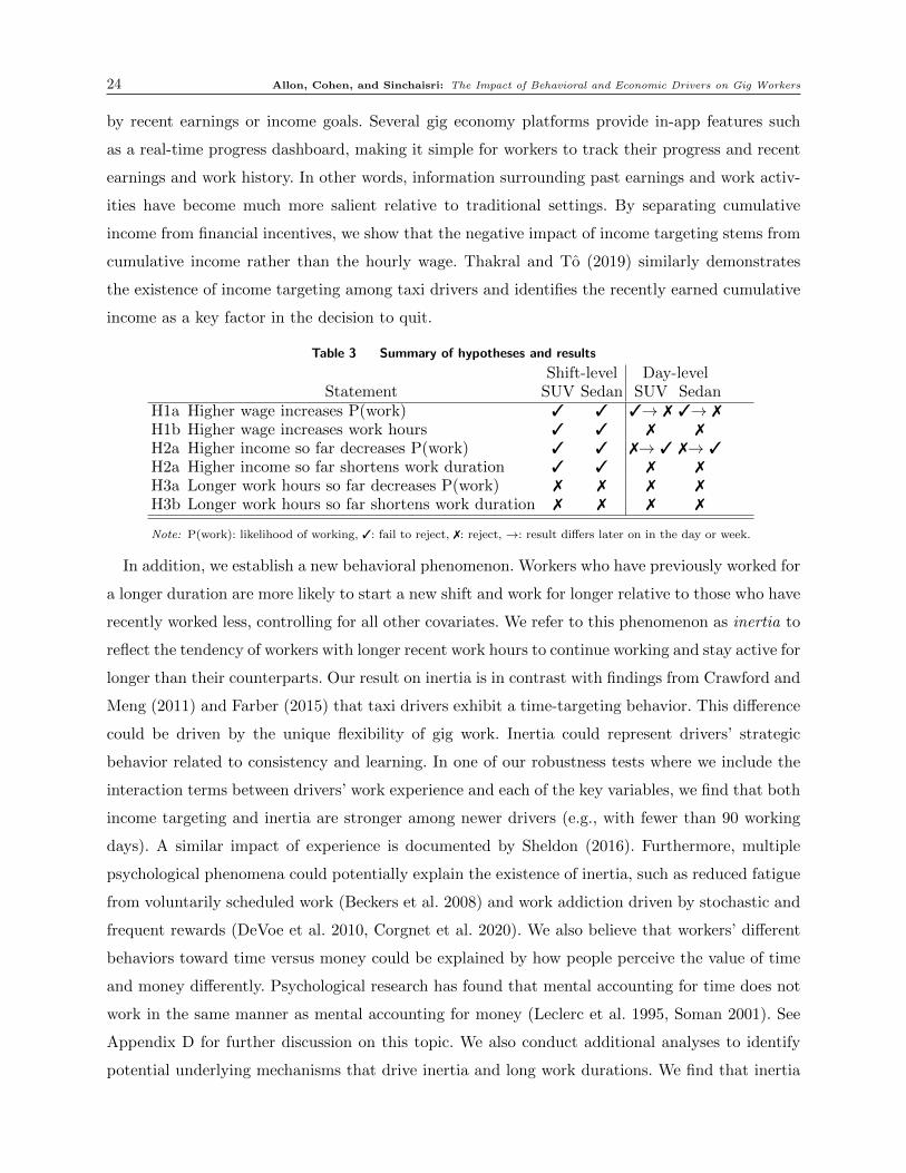
income as a key factor in the decision to quit.
Table 3 Summary of hypotheses and results
Shift-level Day-levelStatement SUV Sedan SUV Sedan
H1a Higher wage increases P(work) 3 3 3→ 7 3→ 7H1b Higher wage increases work hours 3 3 7 7H2a Higher income so far decreases P(work) 3 3 7→ 3 7→ 3H2a Higher income so far shortens work duration 3 3 7 7H3a Longer work hours so far decreases P(work) 7 7 7 7H3b Longer work hours so far shortens work duration 7 7 7 7
Note: P(work): likelihood of working, 3: fail to reject, 7: reject, →: result differs later on in the day or week.
In addition, we establish a new behavioral phenomenon. Workers who have previously worked for
a longer duration are more likely to start a new shift and work for longer relative to those who have
recently worked less, controlling for all other covariates. We refer to this phenomenon as inertia to
reflect the tendency of workers with longer recent work hours to continue working and stay active for
longer than their counterparts. Our result on inertia is in contrast with findings from Crawford and
Meng (2011) and Farber (2015) that taxi drivers exhibit a time-targeting behavior. This difference
could be driven by the unique flexibility of gig work. Inertia could represent drivers’ strategic
behavior related to consistency and learning. In one of our robustness tests where we include the
interaction terms between drivers’ work experience and each of the key variables, we find that both
income targeting and inertia are stronger among newer drivers (e.g., with fewer than 90 working
days). A similar impact of experience is documented by Sheldon (2016). Furthermore, multiple
psychological phenomena could potentially explain the existence of inertia, such as reduced fatigue
from voluntarily scheduled work (Beckers et al. 2008) and work addiction driven by stochastic and
frequent rewards (DeVoe et al. 2010, Corgnet et al. 2020). We also believe that workers’ different
behaviors toward time versus money could be explained by how people perceive the value of time
and money differently. Psychological research has found that mental accounting for time does not
work in the same manner as mental accounting for money (Leclerc et al. 1995, Soman 2001). See
Appendix D for further discussion on this topic. We also conduct additional analyses to identify
potential underlying mechanisms that drive inertia and long work durations. We find that inertia

Allon, Cohen, and Sinchaisri: The Impact of Behavioral and Economic Drivers on Gig Workers 25
is more prevalent among drivers with less experience on the focal platform, or on days when the
financial offers on the focal platform have a high variance, or when the average competition intensity
is high but the variance is low. Detailed discussion and results are reported in Appendix E. Lastly,
we find that gig workers make a decision to work at both shift and day levels, whereas the work
duration appears to be decided at a more granular time unit such as a shift or even an hour.
The latter potentially highlights the unique flexibility of gig jobs that provide workers with full
control of their real-time work schedule. Our results remain valid under a number of robustness
checks, including the following: allowing for non-linear targeting effects, relaxing our assumption on
frequency of target adjustment and definition of shifts, considering instrumental variables for ISF
and HSF , performing alternative sample selection correction, and modeling stopping probabilities
via mixed-effects survival analysis. In summary, with a better understanding of how gig workers
make labor decisions, companies can design more effective incentives and personalize them based
on individual workers’ behaviors.
6. Managerial Implications: Optimal Incentive Allocation
In this section, we illustrate how gig economy firms can use our insights on workers’ behavior to
enhance their operations. We first investigate the benefit of improved incentive allocation based on
two perspectives: (i) increasing service capacity while keeping a fixed budget and (ii) maintaining
the same service capacity at a lower cost. We then further highlight the potential pitfalls of ignoring
behavioral factors and quantify the resulting capacity loss. In Appendix F, we conduct a policy
analysis to demonstrate how our insights can help policymakers evaluate the impact of a regulation.
6.1. Targeted Incentives
Our main results suggest that workers are influenced by their behavioral motives and that the
impact of incentives on the number of active workers may be nonlinear. Targeting specific workers
with different incentives can be beneficial. We examine how the platform can improve its operational
performance by offering personalized incentives based on workers’ attributes. As a benchmark, we
compute the platform’s budget for promotions based on the actual allocation of incentives. We then
re-allocate the promotion budget more efficiently by considering the following two perspectives:
(i) increasing the service capacity (i.e., staffing more workers) using the same budget, and (ii)
maintaining the same service capacity at a lower cost. Our proposed heuristic ranks the workers
by the minimum level of incentives they need to receive in order to start working.
In our context, drivers always receive a guaranteed base pay when they work and sometimes they
receive promotions on top of the base rate. We assume that the budget for promotions is separate
from the budget for base rates. As not every driver who receives a promotion would choose to work,
we compute two types of budgets for promotions. First, we compute the total promotions offered
26 Allon, Cohen, and Sinchaisri: The Impact of Behavioral and Economic Drivers on Gig Workers
to all drivers for every shift on every day in the data as the projected budget. This is the total cost
related to promotions incurred by the platform if all drivers chose to work. Second, we compute
the actual cost based on the realized number of drivers who showed up to work at any given time
as the realized budget. We can then compare the service capacity and cost of our heuristic relative
to the actual allocation. As our data spans one year from October 2016 to September 2017, we
choose the last nine months (January 1–September 30, 2017) as our test set. For each shift on
each day in the test set, we train our model using all observations from the same shift and day of
the week prior to the focal shift. Across 1,012 day-shifts, we observe that 94.59% of drivers were
offered a promotion but only 18.4% of them activated the offer and chose to work. Moreover, 94%
of the drivers who worked did not receive any promotion. These observations suggest that there is
an opportunity to improve the current allocation of financial incentives.
To determine drivers’ baseline probability to work, we first compute the average fraction of
drivers who worked during a given shift on a given weekday using all past data, denoted by D. We
then compute the inverse c.d.f. evaluated at D: D = Φ−1(D), that is, D represents the argument
of Φ(·) in the right hand-side of Equation (6). In other words, D corresponds to the combination
of drivers’ attributes that will induce a probability of working equal to D. For each driver i, we
use all the covariates’ values with the base pay (e.g., excluding promotions) in our fitted model.
This will predict the probability of working when offered only the base rate, pbasei . If pbasei ≥ D,
we label the driver as “driving without promotion.” For other drivers, we compute the difference,
∆i = D− pbasei > 0, to determine the level of additional incentive needed for them to work.
Improving service capacity while keeping the same budget. Assuming that the platform
has a fixed budget for promotions, we consider a strategy to recruit more workers under the same
budget. We first determine the number of drivers who would work regardless of promotions (i.e.,
their base rates are appealing enough to motivate them to work), and then rank the remaining
drivers by increasing values of ∆i. We compute the minimum work-inducing promotion level by
dividing ∆i by the estimated coefficient βoffer. We call this value ∆i. Then, a desired strategy is to
allocate the promotion budget first to drivers with the smallest ∆i until we exhaust the budget or
we can no longer recruit additional drivers. On average, our proposed procedure sends promotions
to 6.27% of all available drivers. The 95% interval for the fraction of drivers who should receive a
promotion is [0.44%, 19.92%]; these fractions are substantially lower than the current practice of
the company. As a result, a much smaller number of drivers would be targeted but each targeted
driver would receive a much more attractive promotion.4 Under the allocation observed in the data,
drivers were offered an average promotion of 0.58× relative to their base rate. Under our proposed
4 One potential concern is fairness. Future research can include additional constraints such as the minimum fractionof drivers receiving a promotion and the maximum number of different promotion levels.

Allon, Cohen, and Sinchaisri: The Impact of Behavioral and Economic Drivers on Gig Workers 27
heuristic, however, targeted drivers receive an average promotion of 2.09×. Ultimately, using the
same budget for promotions, our approach can staff 22.1% additional drivers on average with a
95% interval of [2.46%, 50.50%]. Figure 5 reports the percentage increase in the number of drivers
for each shift and weekday.
Figure 5 Number of additional drivers using our allocation strategy given a fixed budget
10
15
20
25
30
35
Shift of Day
% A
dditio
nal D
rive
rs
Midday PM Peak PM Off Late Night
10
15
20
25
Day of Week%
Additio
nal D
rive
rs
M T W Th F Sa Su
Maintaining service capacity at a lower cost. Companies may have a target level of capacity
they hope to meet for several reasons, such as to satisfy a high forecast demand or maintain low
and reliable wait times. Similar to the previous case, we rank all drivers by increasing values of
the minimum work-inducing promotion level (i.e., ∆i). We subtract the number of drivers who are
predicted to work without any promotion from the desired service capacity. Instead of having a
budget constraint, we now allocate promotions to drivers who require the smallest incentive ∆i
until we reach the desired service capacity. On average, the allocation under our heuristic costs
30.10% less relative to current practice with a 95% interval of [0.75%, 63.54%]. Figure 6 shows the
percentage of cost savings for each shift and weekday.
Figure 6 Simulated cost savings while maintaining the same service capacity
10
20
30
40
50
Shift of Day
% T
ota
l C
ost S
avin
g
Midday PM Peak PM Off Late Night
20
25
30
35
Day of Week
% T
ota
l C
ost S
avin
g
M T W Th F Sa Su

28 Allon, Cohen, and Sinchaisri: The Impact of Behavioral and Economic Drivers on Gig Workers
6.2. Impact of Behavioral Explanations of Labor Decisions
In this section, we quantify the impact of capturing the main behavioral factors obtained in our
estimation results. To this end, we investigate how many workers the platform would fail to attract if
it did not incorporate income targeting and inertia into incentive design. We compare the following
three scenarios to our model:
(a) ISF Only : The firm assumes that work decisions are influenced by ISF but not HSF .
(b) HSF Only : The firm assumes that work decisions are influenced by HSF but not ISF .
(c) Base: The firm ignores both income-targeting and inertia behaviors.
Our analysis is at the day-shift level and reports out-of-sample predictions. The test set consists
of each day-shift between January 1, 2017 and September 30, 2017. For each day-shift in the test
set, we train four separate choice equations—one for each model (a)–(c) above and one for our
model—using all historical observations of the same day-shift from October 2016 to the week prior
to the focal date. Each of the four choice equations represents the predicted outcome depending
on the platform’s assumption on workers’ behavior. We first compute the fraction of drivers’ work
decisions that each model predicts correctly out-of-sample relative to the actual realization in the
data. On average, our model outperforms the other three models in prediction accuracy both at the
shift and day levels. Specifically, when the company ignores behavioral drivers of labor decisions, it
loses 8.6% in prediction accuracy on average. Following the same procedure as in §6.1, we compute
the incentive allocation under each model. More precisely, we first assume that each model is the
true state of the world and solve for the optimal incentive allocation given the promotion budget
observed in the data. Once the allocation is completed, we estimate the expected number of drivers
who would be working, assuming that the true state of the world is actually governed by our model.
Note that by construction, our model will always outperform the other models in terms of expected
capacity. Our main goal here is to quantify the magnitude of capacity loss when the company make
different assumptions about workers’ behavior.
Figure 7 shows that ignoring behavioral factors can lead to a significant loss in the number
of active drivers. Specifically, the Base model leads to an average loss of 16.70% in the expected
number of active drivers relative to our model, with a standard deviation of 13.06%. The ISF
Only (HSF Only) model leads to an average reduction of 9.63% (10.32%) in the expected number
of active drivers with a standard deviation of 9.10% (10.20%).
In summary, these results suggest that it is important for gig platforms to account for income
targeting and inertia. Ignoring these behavioral motives can decrease prediction accuracy, and more
importantly, induce misleading incentive decisions that may result in suboptimal capacity levels.

Allon, Cohen, and Sinchaisri: The Impact of Behavioral and Economic Drivers on Gig Workers 29
Figure 7 Impact of ignoring behavioral factors on the expected number of active drivers
70
80
90
10
0
Shift of Day
% D
rive
rs
Our Model
ISF Only
HSF Only
Base
Midday PM Peak PM Off Late Night
70
80
90
10
0
Day of Week
% D
rive
rs
Our Model
ISF Only
HSF Only
Base
M T W Th F Sa Su
7. Concluding Remarks
The recent rise of the gig economy has changed the way people think about employment. Unlike
traditional employees who work under a fixed schedule, gig economy workers are free to choose
their own schedule and platform to provide service. Such flexibility poses a great challenge to gig
platforms in terms of planning and committing to a service capacity. It also poses a challenge to
policymakers who are concerned about protecting workers. In this paper, we propose a framework
to investigate how gig economy workers make labor decisions. Using data from a ride-hailing
platform, we develop an econometric model that accounts for sample selection and endogeneity
and controls for the competition within the ride-hailing industry. We find that financial incentives
have a positive effect on the decision to work and on the work duration, confirming the positive
income elasticity from the standard income effect. We also observe the influence of behavioral
factors through the accumulated earnings and number of hours previously worked. The dominating
effect, inertia, suggests that the longer workers have been working so far, the more likely they
will continue working and the longer duration they will work for. Our results also reflect a unique
feature of gig work. While workers decide whether to work on both shift and day levels, they
decide on work duration on a shift basis. Finally, our numerical experiments demonstrate that gig
platforms can benefit from incorporating our insights into their incentive optimization.
One of the important phenomena that emerge from this paper is the existence of inertia among
drivers. While we cannot conclude that all gig economy workers exhibit such a behavior, we believe
that it has important implications that go beyond this study. Indeed, we believe that our findings
are generalizable to other flexible workforces. Drivers in our data are not exclusive to the focal
platform and are often working for other gig companies. Policies used by the focal platform are
also quite common in the industry, from delivery to tutoring services. Therefore, there is a lesson
to be learned about the fundamental impact of such policies. Amidst intensifying competition
among providers of similar on-demand services, companies are making every effort to win over a

30 Allon, Cohen, and Sinchaisri: The Impact of Behavioral and Economic Drivers on Gig Workers
mutual pool of workers. This paper empirically identifies several key behavioral factors that affect
gig economy workers’ decisions. These findings can be used to sharpen platforms’ understanding
on how gig economy workers make labor decisions and, ultimately, improve platforms’ operational
decisions (e.g., sending the right offer to the right worker at the right time).
This paper opens several avenues for future research. It could be interesting to validate our
findings by running a controlled field experiment. Given that online platforms routinely run exper-
iments to confirm insights, testing the income targeting and inertia effects could be of interest. A
second direction is to further investigate how workers construct their reference points or targets in
both financial and time dimensions, and how these targets are updated over time. This will allow
companies to gain insights about the (dis)utility of working as well as understanding how work-
ers switch between service providers. Finally, our incentive allocation is based on simple ranking
arguments. Developing a more comprehensive optimization framework to optimize incentives for
each driver in each shift under further operational constraints is also an interesting extension. The
main goals of this research stream would be to refine our understanding of gig economy workers
and develop data-driven methods that can be used by gig platforms to efficiently motivate and
strengthen their relationships with their flexible workforce.
ReferencesAgarwal S, Diao M, Pan J, Sing TF (2015) Are singaporean cabdrivers target earners?, working paper.
Beckers DG, van der Linden D, Smulders PG, Kompier MA, Taris TW, Geurts SA (2008) Voluntary or involuntary?
control over overtime and rewards for overtime in relation to fatigue and work satisfaction. Work & Stress 22(1):33–
50.
Benjaafar S, Ding JY, Kong G, Taylor T (2019) Labor welfare in on-demand service platforms. Available at SSRN
3102736 .
Benjaafar S, Hu M (2020) Operations management in the age of the sharing economy: what is old and what is new?
Manufacturing & Service Operations Management 22(1):93–101.
Bourguignon F, Fournier M, Gurgand M (2007) Selection bias corrections based on the multinomial logit model:
Monte carlo comparisons. Journal of Economic Surveys 21(1):174–205.
Brachet T, David G, Drechsler AM (2012) The effect of shift structure on performance. American Economic Journal:
Applied Economics 4(2):219–46.
Bray RL, Serpa JC, Colak A (2019) Supply chain proximity and product quality. Management science 65(9):4079–
4099.
Cachon GP, Daniels KM, Lobel R (2017) The role of surge pricing on a service platform with self-scheduling capacity.
Manufacturing & Service Operations Management 19(3):368–384.
Camerer C, Babcock L, Loewenstein G, Thaler R (1997) Labor supply of new york city cabdrivers: One day at a
time. The Quarterly Journal of Economics 112(2):407–441.
Carrington WJ (1996) The alaskan labor market during the pipeline era. Journal of Political Economy 104(1):186–218.

Allon, Cohen, and Sinchaisri: The Impact of Behavioral and Economic Drivers on Gig Workers 31
Chen MK, Rossi PE, Chevalier JA, Oehlsen E (2019) The value of flexible work: Evidence from uber drivers. Journal
of Political Economy 127(6):2735–2794.
Chen MK, Sheldon M (2016) Dynamic pricing in a labor market: Surge pricing and flexible work on the uber platform.
EC, 455.
Chen YJ, Dai T, Korpeoglu CG, Korpeoglu E, Sahin O, Tang CS, Xiao S (2020) Om forum—innovative online
platforms: Research opportunities. Manufacturing & Service Operations Management 22(3):430–445.
Collewet M, Sauermann J (2017) Working hours and productivity. Labour Economics 47:96–106.
Corgnet B, Gaechter S, Hernan-Gonzalez R (2020) Working too much for too little: stochastic rewards cause work
addiction. Available at SSRN 3540225 .
Cragg JG (1971) Some statistical models for limited dependent variables with application to the demand for durable
goods. Econometrica (pre-1986) 39(5):829.
Crawford VP, Meng J (2011) New york city cab drivers’ labor supply revisited: Reference-dependent preferences with
rational-expectations targets for hours and income. American Economic Review 101(5):1912–32.
Csikszentmihalyi M, Csikszentmihalyi IS (1992) Optimal experience: Psychological studies of flow in consciousness
(Cambridge university press).
Csikszentmihalyi M, LeFevre J (1989) Optimal experience in work and leisure. Journal of personality and social
psychology 56(5):815.
Dahl GB (2002) Mobility and the return to education: Testing a roy model with multiple markets. Econometrica
70(6):2367–2420.
DeVoe SE, Lee BY, Pfeffer J (2010) Hourly versus salaried payment and decisions about trading time and money
over time. ILR Review 63(4):627–640.
DeVoe SE, Pfeffer J (2007) When time is money: The effect of hourly payment on the evaluation of time. Organizational
Behavior and Human Decision Processes 104(1):1–13.
Dhaene G, Jochmans K (2015) Split-panel jackknife estimation of fixed-effect models. The Review of Economic Studies
82(3):991–1030.
Dong J, Ibrahim R (2020) Managing supply in the on-demand economy: Flexible workers, full-time employees, or
both? Operations Research .
Donohue K, Ozer O, Zheng Y (2020) Behavioral operations: Past, present, and future. Manufacturing & Service
Operations Management 22(1):191–202.
Evans JA, Kunda G, Barley SR (2004) Beach time, bridge time, and billable hours: The temporal structure of
technical contracting. Administrative Science Quarterly 49(1):1–38.
Farber HS (2005) Is tomorrow another day? the labor supply of new york city cabdrivers. Journal of political Economy
113(1):46–82.
Farber HS (2008) Reference-dependent preferences and labor supply: The case of new york city taxi drivers. The
American Economic Review 98(3):1069–1082.
Farber HS (2015) Why you can’t find a taxi in the rain and other labor supply lessons from cab drivers. The Quarterly
Journal of Economics 130(4):1975–2026.

32 Allon, Cohen, and Sinchaisri: The Impact of Behavioral and Economic Drivers on Gig Workers
Farewell V, Long D, Tom B, Yiu S, Su L (2017) Two-part and related regression models for longitudinal data. Annual
review of statistics and its application 4:283–315.
Greene W (2004) Fixed effects and bias due to the incidental parameters problem in the tobit model. Econometric
reviews 23(2):125–147.
Hahn J, Newey W (2004) Jackknife and analytical bias reduction for nonlinear panel models. Econometrica
72(4):1295–1319.
Heckman JJ (1979) Sample selection bias as a specification error. Econometrica: Journal of the econometric society
153–161.
Hu M, Zhou Y (2019) Price, wage and fixed commission in on-demand matching. Available at SSRN 2949513 .
Ibrahim R (2018) Managing queueing systems where capacity is random and customers are impatient. Production
and Operations Management 27(2):234–250.
Imbens G, Wooldridge J (2007) Control function and related methods, what’s new in Econometrics, National Bureau
of Economic Research.
Intelligence E (2019) Freelancing in america: 2019.
Karacaoglu N, Moreno A, Ozkan C (2018) Strategically giving service: The effect of real-time information on service
efficiency. Available at SSRN 3260035 .
Kruzman D (2017) Some uber drivers work dangerously long shifts. URL https://www.usatoday.com/story/money/
cars/2017/07/10/some-uber-drivers-work-dangerously-long-shifts/103090682/.
Leclerc F, Schmitt BH, Dube L (1995) Waiting time and decision making: Is time like money? Journal of Consumer
Research 22(1):110–119.
Levinsohn J, Petrin A (2003) Estimating production functions using inputs to control for unobservables. The Review
of Economic Studies 70(2):317–341.
Madden D (2008) Sample selection versus two-part models revisited: The case of female smoking and drinking. Journal
of health economics 27(2):300–307.
Manyika J, Lund S, Robinson K, Valentino J, Dobbs R (2015) A labor market that works: Connect-
ing talent with opportunity in the digital age. June. McKinsey Global Institute. http://www. mckinsey.
com/˜/media/McKinsey/dotcom/Insights/Employment% 20and% 20growth/Connecting 20.
Mason CH, Perreault Jr WD (1991) Collinearity, power, and interpretation of multiple regression analysis. Journal
of marketing research 28(3):268–280.
Newey WK (1987) Efficient estimation of limited dependent variable models with endogenous explanatory variables.
Journal of Econometrics 36(3):231–250.
Oettinger GS (1999) An empirical analysis of the daily labor supply of stadium vendors. Journal of Political Economy
107(2):360–392.
Okada EM, Hoch SJ (2004) Spending time versus spending money. Journal of consumer research 31(2):313–323.
Puhani P (2000) The heckman correction for sample selection and its critique. Journal of economic surveys 14(1):53–
68.
Sheldon M (2016) Income targeting and the ridesharing market, working paper.

Allon, Cohen, and Sinchaisri: The Impact of Behavioral and Economic Drivers on Gig Workers 33
Soman D (2001) The mental accounting of sunk time costs: Why time is not like money. Journal of Behavioral
Decision Making 14(3):169–185.
Stafford TM (2015) What do fishermen tell us that taxi drivers do not? an empirical investigation of labor supply.
Journal of Labor Economics 33(3):683–710.
Taylor TA (2018) On-demand service platforms. Manufacturing & Service Operations Management 20(4):704–720.
Thakral N, To LT (2019) Daily labor supply and adaptive reference points, american Economic Review.
Watanabe M, Yamauchi K (2016) Psychosocial factors of overtime work in relation to work-nonwork balance: A
multilevel structural equation modeling analysis of nurses working in hospitals. International journal of behavioral
medicine 23(4):492–500.
Wooldridge JM (2015) Control function methods in applied econometrics. Journal of Human Resources 50(2):420–445.

Allon, Cohen, and Sinchaisri: The Impact of Behavioral and Economic Drivers on Gig Workers 1
Appendix A: Additional Details of the Main Results
Figures A1 and A2 provide additional details of the main results from our two-stage model of drivers’
decisions across shifts and across days, respectively. For each of the key variables, we provide the estimated
coefficient and the standard error in parenthesis. Within each model, we also report the estimated coefficient
and the standard error for IMR and two R2 values, total R2 (top) and within R2 (bottom, italicized). We
acknowledge that a few of the IMR estimates are not statistically significant, suggesting that the selection
bias is weak in some cases. However, our insights regarding the impact of financial incentives, cumulative
income, and cumulative work hours on the decisions of both stages are consistent across different model
specifications and selection approaches (e.g., two-part model and Dahl’s correction).
Figure A1 Estimates of our two-stage model of drivers’ shift-level decisions across different shifts
Note: Solid background with bolded text: significantly positive, striped with bolded text: significantly negative,
white with italicized text: non-significant. All at p = 0.05.
Figures A3 provides the effect sizes for an average driver at the shift and day levels, respectively, under
one of the following conditions: (i) a $10 increase in hourly offer or earning rate, (ii) a $10 increase in ISF ,
and (iii) an additional hour to HSF .
Appendix B: Alternative Empirical Approaches
B.1. Sample Selection Bias Correction
B.1.1. Dahl’s correction. Following Dahl (2002) and Bray et al. (2019), we use the selection probability
as a sufficient statistic for the selection bias. Since, in our context, the choice for each driver is only binary: to
work or not, we do not suffer from the curse of dimensionality. Revisiting our level equation (Equation (7)),
f(Houri,t) = β0,i +βwwi,t +βISF ISFi,t +βHSFHSFi,t +βZi,t + θλi,t +ui,t,
we can substitute IMR (λ) with all basis functions of a B-spline by using the quantiles of work probabil-
ities for all drivers, Pwork = [P (Drivei,t = 1|Xi,t),∀i] as interior knots. Let B(Pwork, j) be the jth basis

2 Allon, Cohen, and Sinchaisri: The Impact of Behavioral and Economic Drivers on Gig Workers
Figure A2 Estimates of our two-stage model of drivers’ day-level decisions across different days
Note: Solid background with bolded text: significantly positive, striped with bolded text: significantly negative,
white with italicized text: non-significant. All at p = 0.05.
Figure A3 Effect sizes of changes in hourly financial offer, ISF , and HSF on drivers’ shift-level decisions
Note: Solid background with bolded text: significantly positive, striped with bolded text: significantly negative,
white with italicized text: non-significant. All at p = 0.05.
function of a degree n B-spline with the quantiles of Pwork as m interior knots. Also, we define ηi,t =
ui,t−∑m+n
j=0 γjB(Pwork, j) to maintain the orthogonality of the error term and the expected hours worked.

Allon, Cohen, and Sinchaisri: The Impact of Behavioral and Economic Drivers on Gig Workers 3
Thus, our level equation under this approach becomes:
f(Houri,t) = β0,i +βwwi,t +βISF ISFi,t +βHSFHSFi,t +βZi,t +
m+n∑j=0
γjB(Pwork, j) + ηi,t. (B1)
In Figure B4, we present the estimates for the level equation when choosing m = n = 3. Our results
remain consistent under both approaches for sample selection correction. Note that, for all but sedan drivers’
decisions on Friday and Saturday, the selection variables are significant at p= 0.05, hence confirming that
there exists a selection bias in the decision to work.
Figure B4 Estimates for the level equation using Dahl’s correction
Note: Green background with bolded “+”: significantly positive, yellow with bolded “-”: significantly negative,
white with italicized sign: non-significant. All at p = 0.05.
B.2. Instrumental Variables
B.2.1. Co-skippers IV. This IV follows a similar idea to our main IV, but instead of matching drivers
based on their past work decisions at a specific time in the past, we now match drivers based on the level
of past inactivity. For every day in our data, we categorize drivers into four groups based on each quartile
of the number of consecutive days they have been inactive. We call the drivers of a different vehicle type
who belong to the same group co-skippers. This IV satisfies the relevance condition: Since both the focal
driver and their co-skippers have been inactive for approximately the same time, their incentives should be
highly correlated. From the first stage of our IV estimation, the estimate for the instrument is consistently
signifiant and F-statistics across all models except one are larger than the conventional threshold of 10. This
IV also satisfies the exclusion restriction: Current incentives for co-skippers should not directly influence the
focal driver’s work decision because (i) they drive different vehicle types and (ii) the focal driver does not
have access to co-skippers’ incentives information.
The estimates from shift- and day-level analyses are consistent with our main results. Figure B5 presents
the signs and statistical significance (at p = 0.05) of the estimates across shifts and days. However, these
models are outperformed by our main model both in terms of in-sample and out-of-sample accuracy.

4 Allon, Cohen, and Sinchaisri: The Impact of Behavioral and Economic Drivers on Gig Workers
Figure B5 Estimates across shifts and days using the co-skippers IV
Note: Green background with bolded “+”: significantly positive, yellow with bolded “-”: significantly negative,
white with italicized sign: non-significant. All at p = 0.05.
B.2.2. Hausman-type IV. Inspired by previous studies such as Sheldon (2016), we use the average
hourly offer rate received by all other registered drivers during the same shift on the same day as an instrument
for the offer rate. Similarly, we use the average hourly earning rate earned by all other active drivers during
the same shift on the same day as an instrument for the hourly earning rate. These instruments can be
thought of as a mutual offer or earning rate for eligible drivers in New York City at a particular time. In
addition, the incentives offered to other drivers should not directly influence the focal driver’s decision to
work. Controlling for weather and market conditions using the TLC data, we rule out potential confounders
that affect both the variation in incentives and in labor decisions. Recall that unlike other ride-hailing
platforms, drivers on our platform do not compete with other drivers for promotions as both the base and
promotional rates are decided and announced ahead of time. Moreover, promotions are not offered as a way
to relocate drivers to high-demand areas (see §3.3 for more details). Thus, it suggests that this IV satisfies
the exclusion restriction. The results we obtained using this IV are qualitatively similar as illustrated in
Figure B6. While this type of IV appears to be valid for the choice equation, low F -statistics suggest that it
is a relatively weaker IV relative to both the co-workers and co-skippers IVs.
B.3. Addressing the Multicollinearity Concern
Correlations between ISF and HSF in our data range between 0.667 and 0.928, depending on the time of the
day and the vehicle type. While these correlations appear to be on a high side, we gain sufficient statistical
power by leveraging our large sample size. Based on Mason and Perreault Jr (1991), our levels of collinearity
are between Levels II and III. Given that our R2 is between 0.25 and 0.5, the minimum sample size of 300
is required. In our case, this requirement is readily satisfied since we have over 100,000 observations for each
vehicle type and shift.
Nevertheless, we consider alternative model specifications that still allow us to investigate both the impact
of ISF and HSF on the labor decisions. For conciseness, we present one major approach below. The insights
remain valid in all specifications.

Allon, Cohen, and Sinchaisri: The Impact of Behavioral and Economic Drivers on Gig Workers 5
Figure B6 Estimates across shifts and days using Hausman-type IV
Note: Green with “+”: significantly positive, yellow with “-”: significantly negative, white: non-significant at p = 0.05.
B.3.1. Localized hazard regressions. Motivated by Thakral and To (2019), we estimate additional
models when controlling for drivers who either had the same amount of accumulated earnings or the same
amount of time worked so far. Such a specification allows for a flexible, driver-specific hazard of stopping and
a time-dependent relationship between each of the covariates and the stopping probability. After driving t
trips and accumulating yint from working a total of hint hours, driver i decides to end shift n when the cost
of additional effort exceeds the expected continuation value. The variables yint and hint represent income so
far (ISF ) and hours so far (HSF ) in our setting. We let dint be the decision to stop working after trip t in
shift n. Thakral and To (2019) models the probability that driver i ends shift n at trip t by
P(dint = 1) = f(hint) +β(hint)yint +Xintγ(hint) +µi(hint) + εint,
where f(·) represents the baseline hazard and µ absorbs differences in drivers’ baseline stopping tendencies.
HSF affects the stopping probability through the baseline hazard and the impact of ISF , covariates, and
drivers’ fixed effects. β(h) reflects the effect of an additional dollar of ISF on the probability of ending a
shift for a driver after h hours of work (HSF = h). Thakral and To (2019) employs local linear regressions to
estimate the baseline hazard and the time-varying coefficients by solving a separate weighted least squares
problem:
minα,β,γ,µi
∑i,n,t
w(hint−h)(dint− (αhint +βyint +Xintγ+µi))2
with weights given by w(·). With uniform weights, this procedure becomes fitting a linear model to a localized
subset of data. We consider time windows of different interval: 10, 15, 20, 30, and 60 minutes.
Specifically, we consider the following two models:
(i) HSF impacts how ISF affects the stopping probability. This is similar to the model formulated in
Thakral and To (2019). We model the probability that driver i stops working at time t of day n after
earning ISFint and spending HSFint hours working for the day as:
P(dint = 1) = f(HSFint)+βw(HSFint)wint+βISF (HSFint)ISFint+Xintγ(HSFint)+µi(HSFint)+εint,

6 Allon, Cohen, and Sinchaisri: The Impact of Behavioral and Economic Drivers on Gig Workers
where wint is the hourly financial incentive offered at time t of day n. We include the hourly incentive
to match our main models and reflect the possibility that drivers are less likely to quit if the current
offer is appealing. The local regressions are done by controlling for drivers who were still active at the
population median of HSF .
(ii) ISF impacts how HSF affects the stopping probability. This model is to validate our findings that
drivers exhibit inertia, affecting their work decisions. Using the notation from our setting, we model
the probability that driver i stops working at time t of day n after earning ISFint and spending HSFint
hours working for the day as:
P(dint = 1) = f(ISFint) +βw(ISFint)wint +βHSF (ISFint)HSFint +Xintγ(ISFint) +µi(ISFint) + εint.
The local regressions are done by controlling for drivers who were still active when earning cumulative
income of the population median of ISF .
Results for Model (i): Impact of ISF . The median number of hours that drivers worked on non-
holiday weekdays is 6.72 for SUV drivers and 6.58 for sedan drivers. Table B1 presents the estimates for the
local probit models of the decision to quit within 10, 15, 30, or 60 minutes after reaching the population
median HSF . The results confirm that financial incentives decrease the quitting probability, while cumulative
earnings tend to increase the quitting probability. Under the assumption that cumulative hours worked
(HSF ) only affect the quitting probability through the impact of offers and ISF , we confirm that income
targeting exists while drivers appear to have a positive income elasticity.
Table B1 Estimates of local probit models of quitting decision controlling for cumulative work hours (HSF )
Quit withinSUV Sedan
Offer ISF Offer ISF10 mins −0.0174 0.0004 −0.0340 0.002515 mins −0.0199∗ 0.0014 −0.0365∗ 0.0040∗
30 mins −0.0204∗∗ 0.0023∗ −0.0321∗∗ 0.0039∗∗
1 hour −0.0047 0.0011 −0.0165 0.0016Note: ∗p<0.05; ∗∗p<0.01; ∗∗∗p<0.001
Results for Model (ii): Impact of HSF . We perform a similar analysis where we assume that the
impact of ISF is only through the varying impact of HSF . The median cumulative earnings drivers made
on non-holiday weekdays are $219.73 for SUV drivers and $199.01 for sedan drivers. Table B2 shows that
significant inertia is observed among SUV and sedan drivers when the time window of quitting decision is
between 10 and 30 minutes. We also find that the hourly financial offer consistently decreases the stopping
probability except for large SUV drivers where the effect is the opposite.
B.4. Alternative Construction of ISF and HSF
We first argue that our assumption that the progress toward a daily income or time goal is reset at midnight
is reasonable. 91.07% of drivers’ working days observed in our data do not overlap with midnight (e.g.,
they did not work overnight). Furthermore, 99.93% started working between 5am and 11pm. Therefore, we
believe that drivers consider a new calendar day as a new progress. However, it is plausible that drivers

Allon, Cohen, and Sinchaisri: The Impact of Behavioral and Economic Drivers on Gig Workers 7
Table B2 Estimates of local probit models of quitting decision controlling for cumulative earnings (ISF )
Quit withinSUV Sedan
Offer HSF Offer HSF10 mins −0.18 −0.0652 −0.0047 0.034915 mins −0.0252∗∗∗ −0.1003∗∗∗ −0.0091 0.001930 mins −0.0186∗∗∗ −0.0718∗∗∗ −0.021∗∗∗ −0.1103∗∗∗
1 hour −0.0202∗∗ −0.0235 −0.0182∗∗∗ 0.0228Note: ∗p<0.05; ∗∗p<0.01; ∗∗∗p<0.001
do not reset their weekly goals every Monday. As a robustness study, we relax the assumptions that the
weekly targets are reset every Monday. Instead, drivers might reset the across-day goals only when they start
working after being inactive for some time. In this direction, we analyzed the duration of inactivity between
any consecutive working days. Among 7,800 drivers who worked at least two days in our dataset, the average
number of inactive days between two working days is 2.21. 15% drivers worked everyday on average and
53.30% did not take more than 2 days break. We re-estimated our models by allowing the targets to be reset
every time the drivers did not work for at least two days. Allowing the weekly targets to be reset after taking
time off from work, our original insights remain qualitatively consistent.
Figure B7 Additional competition metrics by hour of day for non-holiday weekdays
(a) Speed: Average speed in miles per hour (b) AggSurge: Number of NYC regions with potential
surge pricing on competing platforms
Appendix C: Competition Among Ride-hailing Platforms
In §4.2.4, we discussed four different metrics to control for unobserved demand for ride-hailing services
and competition effects. Our main results presented in §5 include all observations from October 2016 to
September 2017, the weather information, and the aggregated number of trips on competing platforms
(NumFHV ) as controls for market conditions. For observations between July and September 2017, we
conduct an additional analysis to further include Speed and AggSurge as covariates. Figures B7a and B7b
illustrate the variations in Speed and AggSurge by hour of day for non-holiday weekdays, respectively. These
new results are qualitatively consistent with our main results. Tables C3 and C4 display the estimates for
the first-stage estimation of whether or not to work for each shift. We observe a generally positive income

8 Allon, Cohen, and Sinchaisri: The Impact of Behavioral and Economic Drivers on Gig Workers
elasticity, income targeting behavior, and inertia throughout all the shifts. Speed appears to have a negative
impact on the decision to work in general, suggesting that drivers are less likely to work for the focal platform
when there is less traffic. The aggregated surge has also a negative impact on the decision to work. This is
to be expected: given that the financial incentive for the focal platform is fixed and known, drivers are less
likely to work when the outside option is more appealing.
Table C3 Estimates for the shift-level first-stage estimation for sedan drivers during Summer 2017
Sedan Offer ISF HSF Speed AggSurgeMid-day 0.0075*** -0.0354** 3.6385*** -0.0298 -2.9551***PM peak -0.0209*** -0.0016* 0.4743*** -0.0536** -3.9532***PM off-peak 0.0136*** -0.0034*** 0.413*** 0.0132 -1.1326**Late night 0.01079** -0.004*** 0.38036*** -0.07055*** -0.51665Note: ∗p<0.05; ∗∗p<0.01; ∗∗∗p<0.001
Table C4 Estimates for the shift-level first-stage estimation for SUV drivers during Summer 2017
SUV Offer ISF HSF Speed AggSurgeMid-day 0.0035** -0.0535*** 4.3936*** 0.0007 -2.5716***PM peak -0.0433*** -0.0024*** 0.5249*** -0.0563*** -3.6690***PM off-peak 0.0028 -0.0024*** 0.3414*** -0.0121 -0.2124Late night 0.0085*** -0.0023*** 0.2945*** -0.0785*** 0.0920Note: ∗p<0.05; ∗∗p<0.01; ∗∗∗p<0.001
The results for the second stage are relatively consistent as well (see Tables C5 and C6). Higher hourly
earnings appear to be associated with a longer work duration for most shifts. Income targeting behavior
becomes less significant. Inertia is stronger earlier on in the day. Finally, we observe that, conditional on
driving for the shift, drivers are less influenced by the traffic conditions or by the potential surge pricing
from other platforms.
Table C5 Estimates for the shift-level second-stage estimation for sedan drivers during Summer 2017
Sedan Earnings ISF HSF Speed AggSurge IMRMid-day 0.008 -0.019*** 1.604*** -0.039 0.0003 ***PM peak 0.025* -0.001 0.084*** 0.012 0.029 ***PM off-peak 0.003 -0.003*** 0.006 -0.0001 0.147 ***Late night 0.03*** 0.001 -0.071** 0.019 0.11* ***Note: ∗p<0.05; ∗∗p<0.01; ∗∗∗p<0.001
Table C6 Estimates for the shift-level second-stage estimation for SUV drivers during Summer 2017
SUV Earnings ISF HSF Speed AggSurge IMRMid-day -0.001 -0.008 1.819*** -0.034 -1.008 ***PM peak 0.062*** -0.0002 0.245*** -0.053*** -0.421 ***PM off-peak 0.004*** -0.0002* 0.033*** -0.002 -0.027 ***Late night 0.022*** 0.0001 0.021 -0.006 0.843Note: ∗p<0.05; ∗∗p<0.01; ∗∗∗p<0.001

Allon, Cohen, and Sinchaisri: The Impact of Behavioral and Economic Drivers on Gig Workers 9
For the day-level analysis, we find that, in the first-stage estimation, positive income elasticity and income
targeting behavior became less apparent. Sedan drivers responded positively to the hourly offer from Tuesday
to Thursday, whereas SUV drivers did not. The effect of cumulative earnings is generally insignificant, except
a sign of income targeting at the end of the week. However, inertia is still significant and apparent for most
days, Thursday through Sunday for sedan driver, and Wednesday through Sunday for SUV drivers. Lastly,
for the second-stage estimation, we find no significant estimates for our key variables. This is in line with
our original results, which led us to conclude that the decision on the work duration for the day was not
determined at the beginning of the day.
Appendix D: Psychological Explanations for Our Main Results
Our main results suggest that workers on our focal platform exhibit different behaviors regarding cumulative
earnings and recent work duration. We believe such different behaviors stem from the fact that people
perceive the value of time and money differently. Contrary to a common saying that time is money, empirical
research from psychology shows that decisions about time follow different rules than decisions about money.
For example, Leclerc et al. (1995) finds that people are more averse to uncertainty with time as contrasted
with money. In other words, people are risk averse with respect to decisions in the domain of time loss despite
being risk-seeking with respect to decisions involving monetary loss. The authors concluded that because
time is less substitutable than money, being certain is more important for decisions about time, and people
are more averse when there is uncertainty about the allocation of time. Soman (2001) shows that people
do not mentally account for their time in the same way as they account for money as the former is more
difficult, while Okada and Hoch (2004) demonstrates that people spend time in a systematically different
way from spending money because the value of time is of greater ambiguity. The distinction of attitude
toward time and money applies to work motivation and decisions as well. Workers who can adjust their own
work schedules are found to be influenced by internal reference targets. Depending on the context, workers
may form only a target for income (Camerer et al. 1997), a target for time (Farber 2015), both in the same
direction (Crawford and Meng 2011), or both in the opposite direction as observed in our work. DeVoe
and Pfeffer (2007) shows that organizational practices such as how firms pay their employees may influence
employees’ psychological evaluation of time and the tradeoffs they make between time and money.
Our key insight suggests that gig economy workers may exhibit inertia at work. In our context, inertia
refers to the positive correlation between the recent work duration and the decision to start a new work
shift. We have identified the following three potential explanations of inertia from the fields of psychology,
organizational behavior, and management.
(i) First, inertia could be linked to the concept of experience of flow from positive psychology. A flow
state is the mental state in which a person performing an activity is fully immersed in a feeling of
energized focus, full involvement, and enjoyment in the process of the activity (Csikszentmihalyi and
Csikszentmihalyi 1992). The complete absorption into the activity affects how the person perceives
the sense of time, leading to a continuation of performing the task even though the marginal benefit
is negligible. Flow theory postulates key conditions required to achieve a flow state. These conditions
include clear goals and task structure, clear and immediate performance feedback, a balance between

10 Allon, Cohen, and Sinchaisri: The Impact of Behavioral and Economic Drivers on Gig Workers
the challenges of the task and one’s own skills, one’s feeling of control, and one’s intrinsic motivation.
Gig economy workers are likely to meet these conditions since gig tasks typically have a known set of
goals and structure, feedback (e.g., from customers) and compensation are provided frequently, and
workers are generally skilled at the particular tasks and have some control over their decisions (e.g.,
work schedule). Csikszentmihalyi and LeFevre (1989) suggests that flow can be experienced in both
work and leisure settings, but more dominantly in the former. Among different leisure activities, the
authors find that driving is the most common task that generates the flow experience. This finding
fits well with our analysis of ride-hailing drivers. Therefore, it is possible that drivers on our platform
are more likely to work if they recently worked for a longer duration because they are more likely to
experience the flow state.
(ii) Second, inertia may reflect work addiction caused by stochastic rewards. Applying insights from neu-
roscience research that stochastic rewards could act as a motivator, Corgnet et al. (2020) conducts a
series of behavioral experiments to investigate the relationship between stochastic rewards and workers’
likelihood to quit working on effortful tasks. The authors found that participants who were offered a
stochastic rate of compensation stayed working for a longer period than those offered a deterministic
rate. The persistence on the tasks is linked to stress generated by the uncertainty. In a gig economy
setting, compensation to workers is typically determined in response to real-time market conditions
(e.g., demand) and depends on the specific task and workers’ performance. Work addiction among gig
workers has been documented and attributed to the rate of compensation (Kruzman 2017). For our
focal platform, financial incentives are decided and communicated to drivers ahead of time, but drivers’
opportunity costs (e.g., incentives from competing platforms) are not deterministic. Therefore, it is
possible that inertia is related to workaholism driven by uncertain rewards.
(iii) Third, inertia, as the absence of fatigue, could be associated with gig workers’ flexibility in deciding
work schedule. Watanabe and Yamauchi (2016) shows that when workers voluntarily opted to work
for a longer period, there is a positive effect on their work-life balance due to the enjoyment of the
work itself or increased rewards. Having control over work duration and being compensated for the
work are found to be important for workers’ satisfaction. Similarly, workers who voluntarily chose to
work overtime did not feel more fatigued but instead felt satisfied as long as they chose their own
schedule (Beckers et al. 2008). Although the concept of overtime work can only be applied loosely to
gig workers since they have full control of their entire schedule, these findings highlight the potential
beneficial impact of the flexibility to choose one’s own work schedule: reduced fatigued and increased
satisfaction. A study on technical contractors whose schedule were not decided by the organization
shows that, despite having full control over their work schedule and perceiving the privileged flexibility,
these contractors chose to work long hours and appeared to follow a less flexible schedule (Evans et al.
2004). They considered leisure time as a period of loss without pay and hence they sought to minimize
time away from work. Using the British Household Panel Survey, DeVoe et al. (2010) observes that
individuals who received hourly wage are more willing to trade their leisure time to work and earn
more money than those receiving a salary pay. Putting these findings together, we conclude that in

Allon, Cohen, and Sinchaisri: The Impact of Behavioral and Economic Drivers on Gig Workers 11
our setting where workers can freely choose their own work schedule and receive a hourly pay, they are
more likely to work for longer, become more satisfied with long work hours, and feel less fatigue.
Appendix E: Potential Mechanisms for Behavioral Effects
We conduct additional analyses to identify potential underlying mechanisms that drive income targeting and
inertia. First, we test whether experience on the platform moderates inertia as well as labor supply elasticity
and income targeting. We replicate some of the findings from Sheldon (2016) on whether experience affects
labor supply elasticity. Since our data spans one full year (October 2016–September 2017), and there is no
information on the date at which each driver joined the platform, we only consider drivers who joined the
platform for the first time within our data (e.g., started after October 10, 2016 but before September 30,
2017) for this analysis. We then measure the experience of each remaining driver by splitting the observations
into bins of working days in increments of ten, that is, the first ten days that the driver works for the platform
correspond to the first bin, days eleven to twenty correspond to the next bin, and so forth until the last bin
which consists of days 260 to 270. Overall, there are 27 different bins. These bins of experience levels are
included as dummy variables as well as the interaction term with the instrument, capturing the marginal
effect on the elasticity.
Following the specification used in Sheldon (2016), we find that the income elasticities are positive and
do not appear to be affected by experience (see Table E7 (i) below). However, when including the other key
variables, ISF and HSF , we infer the impact of experience as follows. For the income elasticities, controlling
for ISF and HSF , we observe a positive but noisy trend in the impact of experience. Notably, elasticities
after 100 days of work are higher than those of early work days. The negative impact of ISF and the positive
impact of HSF are significant and with a larger magnitude for the first 80 days of work compared to later.
This suggests that drivers with more experience working on the focal platform exhibit less income targeting
and inertia relative to the drivers who just started out, similar to the findings in Sheldon (2016). Table E7 (ii)
illustrates this result for the first 150 working days. Therefore, inertia could reflect learning on the platform:
the longer a driver has worked recently means that s/he has gained more information that motivates her/him
to work more later on. Such learning of new information becomes less important as the driver has gained
more experience working on the platform.
Finally, we identify potential associations between long daily work hours that could have been triggered
by inertia and driver experience as well as market conditions. Specifically, we regress the daily work hours
on these factors for driver-dates where we observe inertia and control for driver and time fixed effects. As
illustrated in Table E8, we find that inertia is more prevalent among drivers with less experience on the focal
platform, or on days when the financial offers on the focal platform have a low mean but a high variance
across shifts, or when the average competition intensity is high but the variance is low. While these findings
only provide correlational evidence, we believe that they are useful in guiding future researchers to further
investigate mechanisms underlying inertia.
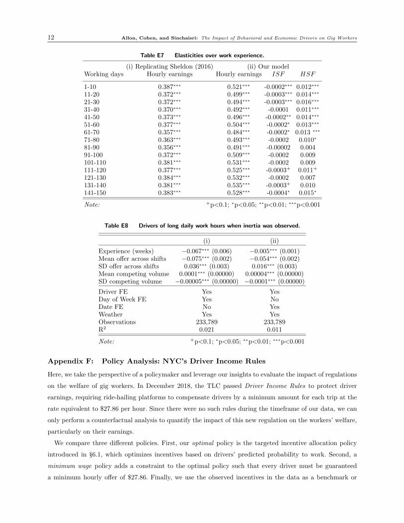
12 Allon, Cohen, and Sinchaisri: The Impact of Behavioral and Economic Drivers on Gig Workers
Table E7 Elasticities over work experience.
(i) Replicating Sheldon (2016) (ii) Our modelWorking days Hourly earnings Hourly earnings ISF HSF
1-10 0.387∗∗∗ 0.521∗∗∗ -0.0002∗∗∗ 0.012∗∗∗
11-20 0.372∗∗∗ 0.499∗∗∗ -0.0003∗∗∗ 0.014∗∗∗
21-30 0.372∗∗∗ 0.494∗∗∗ -0.0003∗∗∗ 0.016∗∗∗
31-40 0.370∗∗∗ 0.492∗∗∗ -0.0001 0.011∗∗∗
41-50 0.373∗∗∗ 0.496∗∗∗ -0.0002∗∗ 0.014∗∗∗
51-60 0.377∗∗∗ 0.504∗∗∗ -0.0002∗ 0.013∗∗∗
61-70 0.357∗∗∗ 0.484∗∗∗ -0.0002∗ 0.013 ∗∗∗
71-80 0.363∗∗∗ 0.493∗∗∗ -0.0002 0.010∗
81-90 0.356∗∗∗ 0.491∗∗∗ -0.00002 0.00491-100 0.372∗∗∗ 0.509∗∗∗ -0.0002 0.009101-110 0.381∗∗∗ 0.531∗∗∗ -0.0002 0.009111-120 0.377∗∗∗ 0.525∗∗∗ -0.0003+ 0.011+
121-130 0.384∗∗∗ 0.532∗∗∗ -0.0002 0.007131-140 0.381∗∗∗ 0.535∗∗∗ -0.0003+ 0.010141-150 0.383∗∗∗ 0.528∗∗∗ -0.0004∗ 0.015∗
Note: +p<0.1; ∗p<0.05; ∗∗p<0.01; ∗∗∗p<0.001
Table E8 Drivers of long daily work hours when inertia was observed.
(i) (ii)
Experience (weeks) −0.067∗∗∗ (0.006) −0.005∗∗∗ (0.001)Mean offer across shifts −0.075∗∗∗ (0.002) −0.054∗∗∗ (0.002)SD offer across shifts 0.036∗∗∗ (0.003) 0.016∗∗∗ (0.003)Mean competing volume 0.0001∗∗∗ (0.00000) 0.00004∗∗∗ (0.00000)SD competing volume −0.00005∗∗∗ (0.00000) −0.0001∗∗∗ (0.00000)
Driver FE Yes YesDay of Week FE Yes NoDate FE No YesWeather Yes YesObservations 233,789 233,789R2 0.021 0.011
Note: +p<0.1; ∗p<0.05; ∗∗p<0.01; ∗∗∗p<0.001
Appendix F: Policy Analysis: NYC’s Driver Income Rules
Here, we take the perspective of a policymaker and leverage our insights to evaluate the impact of regulations
on the welfare of gig workers. In December 2018, the TLC passed Driver Income Rules to protect driver
earnings, requiring ride-hailing platforms to compensate drivers by a minimum amount for each trip at the
rate equivalent to $27.86 per hour. Since there were no such rules during the timeframe of our data, we can
only perform a counterfactual analysis to quantify the impact of this new regulation on the workers’ welfare,
particularly on their earnings.
We compare three different policies. First, our optimal policy is the targeted incentive allocation policy
introduced in §6.1, which optimizes incentives based on drivers’ predicted probability to work. Second, a
minimum wage policy adds a constraint to the optimal policy such that every driver must be guaranteed
a minimum hourly offer of $27.86. Finally, we use the observed incentives in the data as a benchmark or
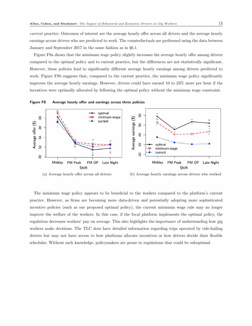
Allon, Cohen, and Sinchaisri: The Impact of Behavioral and Economic Drivers on Gig Workers 13
current practice. Outcomes of interest are the average hourly offer across all drivers and the average hourly
earnings across drivers who are predicted to work. The counterfactuals are performed using the data between
January and September 2017 in the same fashion as in §6.1.
Figure F8a shows that the minimum wage policy slightly increases the average hourly offer among drivers
compared to the optimal policy and to current practice, but the differences are not statistically significant.
However, these policies lead to significantly different average hourly earnings among drivers predicted to
work. Figure F8b suggests that, compared to the current practice, the minimum wage policy significantly
improves the average hourly earnings. However, drivers could have earned 10 to 23% more per hour if the
incentives were optimally allocated by following the optimal policy without the minimum wage constraint.
Figure F8 Average hourly offer and earnings across three policies
(a) Average hourly offer across all drivers (b) Average hourly earnings across drivers who worked
The minimum wage policy appears to be beneficial to the workers compared to the platform’s current
practice. However, as firms are becoming more data-driven and potentially adopting more sophisticated
incentive policies (such as our proposed optimal policy), the current minimum wage rule may no longer
improve the welfare of the workers. In this case, if the focal platform implements the optimal policy, the
regulation decreases workers’ pay on average. This also highlights the importance of understanding how gig
workers make decisions. The TLC does have detailed information regarding trips operated by ride-hailing
drivers but may not have access to how platforms allocate incentives or how drivers decide their flexible
schedules. Without such knowledge, policymakers are prone to regulations that could be suboptimal.