the icdar/grec 2013 music scores competition: staff removal

HAL Id: hal-01006118https://hal.archives-ouvertes.fr/hal-01006118

Submitted on 13 Jun 2014

HAL is a multi-disciplinary open accessarchive for the deposit and dissemination of sci-entific research documents, whether they are pub-lished or not. The documents may come fromteaching and research institutions in France orabroad, or from public or private research centers.

L’archive ouverte pluridisciplinaire HAL, estdestinée au dépôt et à la diffusion de documentsscientifiques de niveau recherche, publiés ou non,émanant des établissements d’enseignement et derecherche français ou étrangers, des laboratoirespublics ou privés.

The ICDAR/GREC 2013 Music Scores Competition:Staff Removal

Alicia Fornés, Van Cuong Kieu, Muriel Visani, Nicholas Journet, Dutta Anjan

To cite this version:Alicia Fornés, Van Cuong Kieu, Muriel Visani, Nicholas Journet, Dutta Anjan. The ICDAR/GREC2013 Music Scores Competition: Staff Removal. Lecture notes in computer science, springer, 2014,pp.1-16. <hal-01006118>

https://hal.archives-ouvertes.fr/hal-01006118

https://hal.archives-ouvertes.fr

The ICDAR/GREC 2013 Music Scores

Competition: Staff Removal

Alicia Fornes1, V.C. Kieu2,3, Muriel Visani2, Nicholas Journet3, and AnjanDutta1

1Computer Vision Center - Dept. of Computer Science,Universitat Autonoma de Barcelona, Ed.O, 08193, Bellaterra, Spain

2 Laboratoire Informatique, Image et Interaction - L3iUniversity of La Rochelle, La Rochelle, France

3 Laboratoire Bordelais de Recherche en InformatiqueLaBRI, University of Bordeaux I, Bordeaux, France

[email protected], [email protected], {vkieu, journet}@labri.fr

Abstract. The first competition on music scores that was organized atICDAR and GREC in 2011 awoke the interest of researchers, who partic-ipated in both staff removal and writer identification tasks. In this secondedition, we focus on the staff removal task and simulate a real case sce-nario: old and degraded music scores. For this purpose, we have generateda new set of images using two degradations: local noise and 3D distor-tions. In this paper we provide an extended description of the dataset,degradation methods, evaluation metrics, the participant’s methods andthe obtained results that could not be presented in ICDAR and GRECproceedings due to page limitations.

1 Introduction

The recognition of music scores has been an active research field for decades [1,2]. Many researchers in Optical Music Recognition have proposed staff removalalgorithms in order to make easier the segmentation and enhance the accuracy ofmusic symbol recognition [3, 4]. However, the staff removal task cannot be con-sidered as a solved problem, especially when dealing with degraded handwrittenmusic scores. This task is even defined as one of the ”three challenges that shouldbe addressed in future work on OMR as applied to manuscript scores” in the2012 survey of Rebelo et al. [2].

At ICDAR [5] and GREC 2011, we organized the first edition of the musicscores competition. For the staff removal task, we created several sets of dis-torted images in order to test the robustness of the staff removal algorithms.Each set corresponded to a different kind of distortion (e.g. Kanungo noise, ro-tation, curvature, staffline interruption, typeset emulation, staffline y-variation,staffline thickness ratio, staffline thickness variation and white speckles). Thestaff removal competition woke up the interest of researchers, with eight submit-ted participant methods. Most staff removal methods showed good performance

2 Alicia Fornes, V.C Kieu, Muriel Visani, Nicholas Journet, Anjan Dutta

in front of severe distorted images, although the detection of the staff lines stillneeded o be improved.

After GREC 2011, we extended the staff removal competition [6]. The goalwas to simulate a real scenario, in which music scores usually contain more thanone single kind of distortion. For this purpose, we combined some of the ICDAR2011 distortions at different levels to create new sets of degraded images. Wethen asked the participants to run their algorithms on this new set of images.Unsurprisingly, the new results demonstrated that the performances of mostmethods were significantly decreased because of the combination of distortions.

By organizing a second edition of this competition at ICDAR / GREC 2013,we aimed at fostering the interest of researchers and focusing on the challeng-ing problem of old document image analysis and recognition. For this secondedition, we have generated realistic semi-synthetic images that emulate typicaldegradations appearing in old handwritten documents such as local noise and3D distortions.

The rest of the paper is organized as follows. Firstly, we will describe theoriginal dataset, the degradation models, and the generated training and testsets. Then, we will present the participants’ methods. Finally, we will detail thethe evaluation metrics, the results analysis, and conclude the paper.

2 Database

In this section we describe the original database, the degradation methods, andthe semi-synthetic database for the competition.

2.1 Original CVC-MUSCIMA database

The original CVC-MUSCIMA 1 database [7] consists of 1,000 handwritten musicscore images, written by 50 different musicians. The 50 writers are adult mu-sicians, in order to ensure that they have their own characteristic handwritingmusic style. Each writer has transcribed exactly the same 20 music pages, usingthe same pen and kind of music paper. The 20 selected music sheets containmusic scores for solo instruments, choir or orchestra.

2.2 Degradation Models

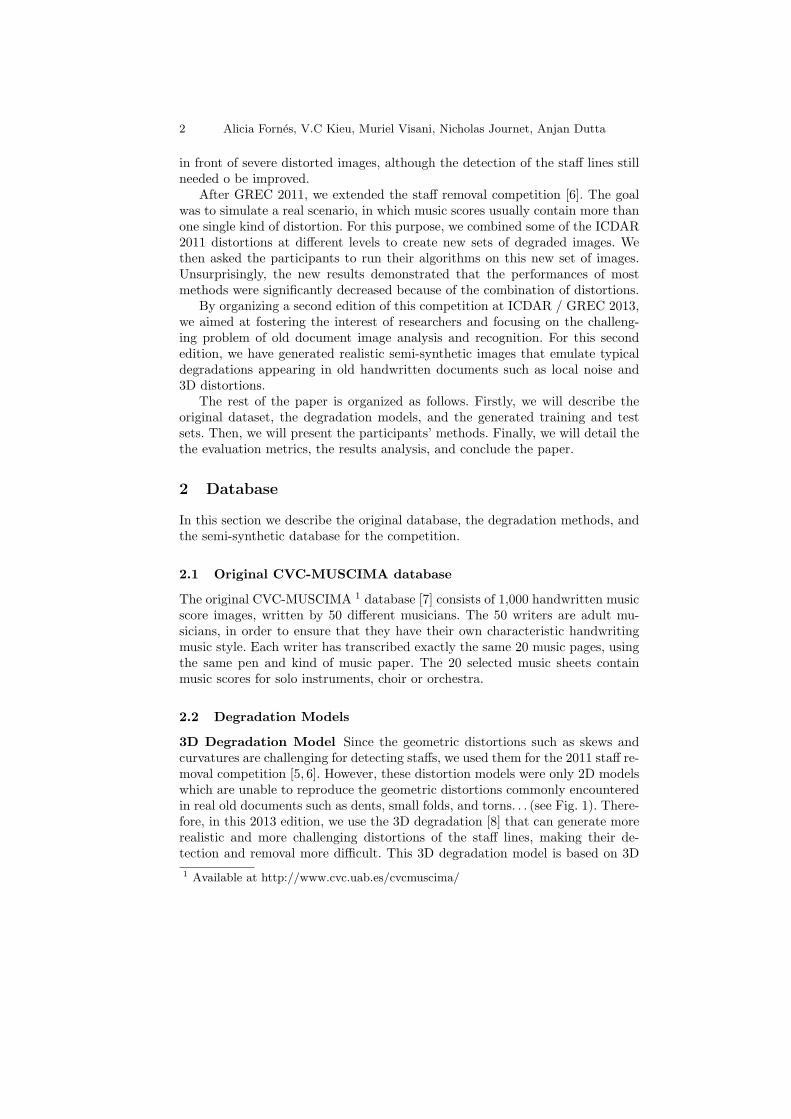
3D Degradation Model Since the geometric distortions such as skews andcurvatures are challenging for detecting staffs, we used them for the 2011 staff re-moval competition [5, 6]. However, these distortion models were only 2D modelswhich are unable to reproduce the geometric distortions commonly encounteredin real old documents such as dents, small folds, and torns. . . (see Fig. 1). There-fore, in this 2013 edition, we use the 3D degradation [8] that can generate morerealistic and more challenging distortions of the staff lines, making their de-tection and removal more difficult. This 3D degradation model is based on 3D

1 Available at http://www.cvc.uab.es/cvcmuscima/

The ICDAR/GREC 2013 Music Scores Competition: Staff Removal 3

meshes and texture coordinate generation. It can wrap any 2D (flat) image ofa document on a 3D mesh acquired by scanning a non-flat old document usinga 3D scanner. The wrapping functions we use are specifically adapted to docu-ment images. In our case, we wrap the original music score images on different3D meshes. For more details, please refer to [8].

Curve Convexo-concave Dent

Fold Skew Torn

Fig. 1: Geometric distortions in real document images

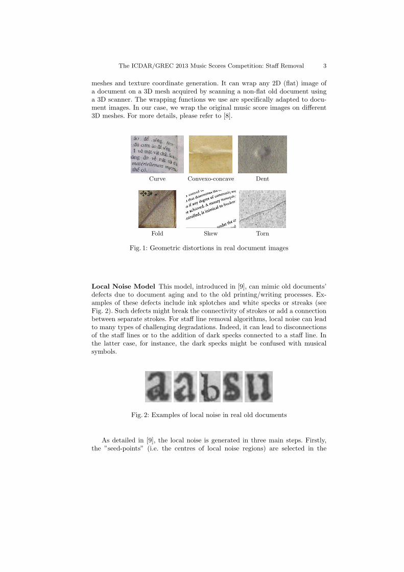
Local Noise Model This model, introduced in [9], can mimic old documents’defects due to document aging and to the old printing/writing processes. Ex-amples of these defects include ink splotches and white specks or streaks (seeFig. 2). Such defects might break the connectivity of strokes or add a connectionbetween separate strokes. For staff line removal algorithms, local noise can leadto many types of challenging degradations. Indeed, it can lead to disconnectionsof the staff lines or to the addition of dark specks connected to a staff line. Inthe latter case, for instance, the dark specks might be confused with musicalsymbols.

Fig. 2: Examples of local noise in real old documents

As detailed in [9], the local noise is generated in three main steps. Firstly,the ”seed-points” (i.e. the centres of local noise regions) are selected in the


neighborhood of connected components’ borders (obtained by binarizing theinput grayscale image). Then, we define an arbitrary noise region at each seed-point (in our case, its shape is an ellipse). Finallly, the grey-level values of thepixels inside the noise regions are modified so as to obtain realistic looking brightand dark specks, and mimic defects due to the age of the document (ink fading,paper degradation...) and writing process (ink drops).

2.3 Degraded Database

For comparing the robustness of the staff removal algorithms proposed by theparticipants to this competition, we degrade the original CVC-MUSCIMA databaseusing the two degradation models presented in Section 2.2. As a result, we obtaina semi-synthetic database that consists of 4000 images in the training set and2000 images in the test set.

Training Set It consists in 4000 semi-synthetic images generated from 667 outof the 1000 original images. This set is split into the three following subsets:

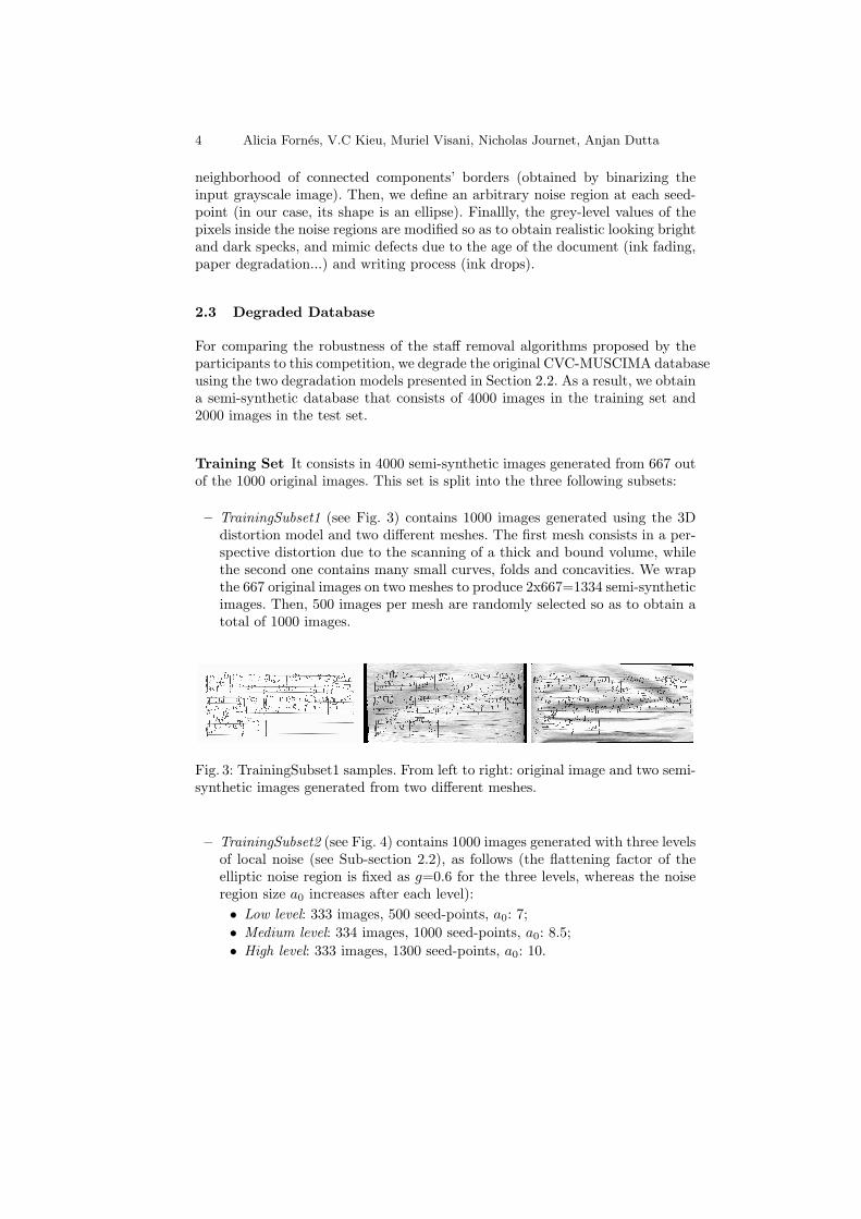
– TrainingSubset1 (see Fig. 3) contains 1000 images generated using the 3Ddistortion model and two different meshes. The first mesh consists in a per-spective distortion due to the scanning of a thick and bound volume, whilethe second one contains many small curves, folds and concavities. We wrapthe 667 original images on two meshes to produce 2x667=1334 semi-syntheticimages. Then, 500 images per mesh are randomly selected so as to obtain atotal of 1000 images.

Fig. 3: TrainingSubset1 samples. From left to right: original image and two semi-synthetic images generated from two different meshes.

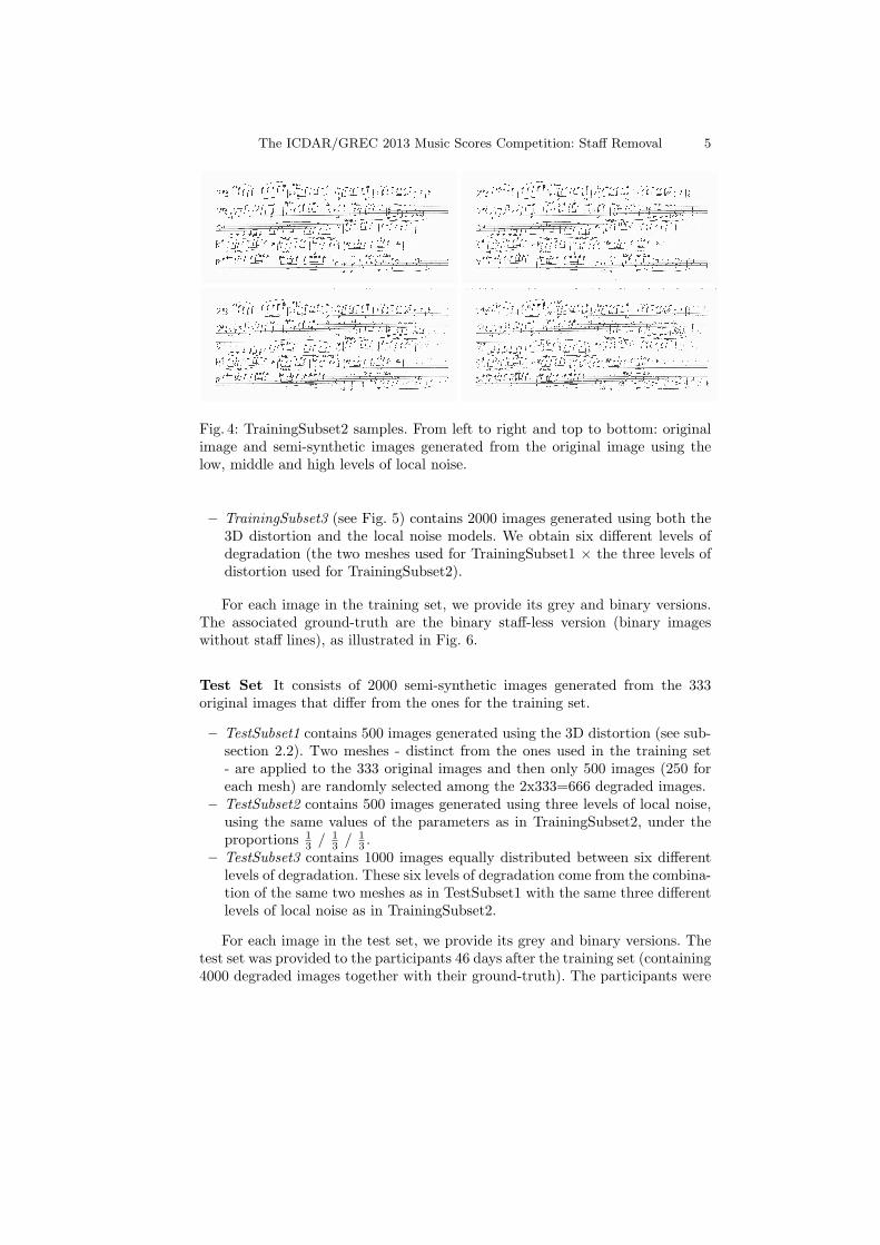
– TrainingSubset2 (see Fig. 4) contains 1000 images generated with three levelsof local noise (see Sub-section 2.2), as follows (the flattening factor of theelliptic noise region is fixed as g=0.6 for the three levels, whereas the noiseregion size a0 increases after each level):

• Low level: 333 images, 500 seed-points, a0: 7;

• Medium level: 334 images, 1000 seed-points, a0: 8.5;

• High level: 333 images, 1300 seed-points, a0: 10.


Fig. 4: TrainingSubset2 samples. From left to right and top to bottom: originalimage and semi-synthetic images generated from the original image using thelow, middle and high levels of local noise.

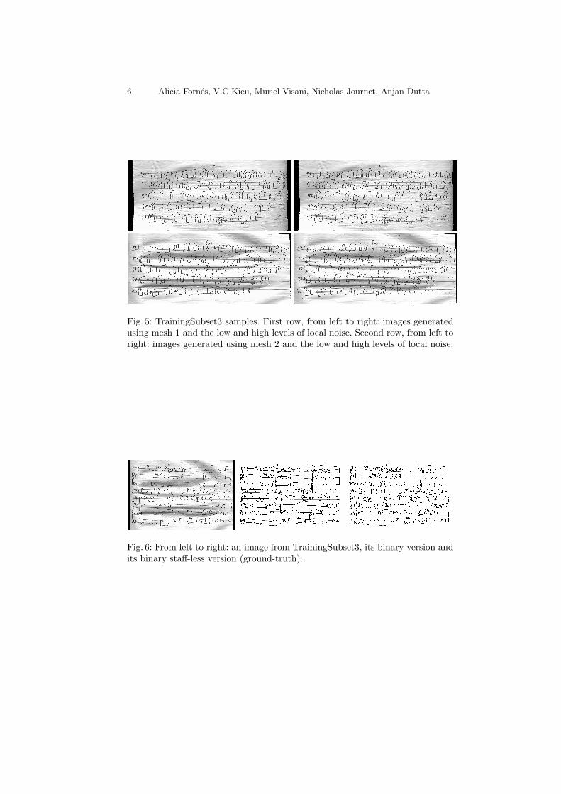
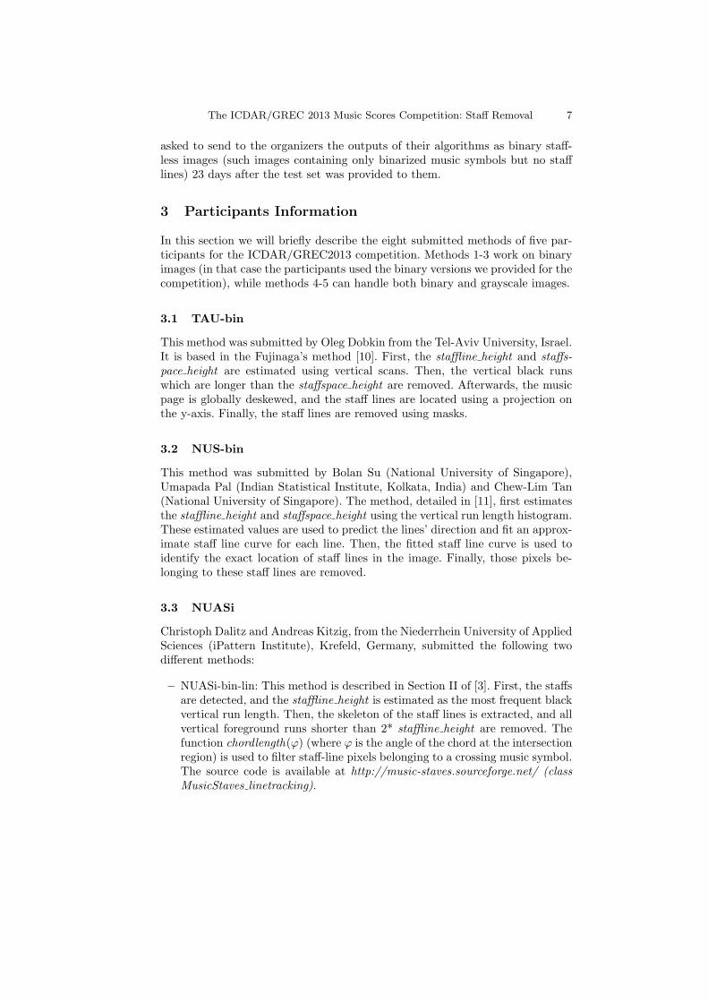
– TrainingSubset3 (see Fig. 5) contains 2000 images generated using both the3D distortion and the local noise models. We obtain six different levels ofdegradation (the two meshes used for TrainingSubset1 × the three levels ofdistortion used for TrainingSubset2).

For each image in the training set, we provide its grey and binary versions.The associated ground-truth are the binary staff-less version (binary imageswithout staff lines), as illustrated in Fig. 6.

Test Set It consists of 2000 semi-synthetic images generated from the 333original images that differ from the ones for the training set.

– TestSubset1 contains 500 images generated using the 3D distortion (see sub-section 2.2). Two meshes - distinct from the ones used in the training set- are applied to the 333 original images and then only 500 images (250 foreach mesh) are randomly selected among the 2x333=666 degraded images.

– TestSubset2 contains 500 images generated using three levels of local noise,using the same values of the parameters as in TrainingSubset2, under theproportions 1

3/ 1

3/ 1

3.

– TestSubset3 contains 1000 images equally distributed between six differentlevels of degradation. These six levels of degradation come from the combina-tion of the same two meshes as in TestSubset1 with the same three differentlevels of local noise as in TrainingSubset2.

For each image in the test set, we provide its grey and binary versions. Thetest set was provided to the participants 46 days after the training set (containing4000 degraded images together with their ground-truth). The participants were


Fig. 5: TrainingSubset3 samples. First row, from left to right: images generatedusing mesh 1 and the low and high levels of local noise. Second row, from left toright: images generated using mesh 2 and the low and high levels of local noise.

Fig. 6: From left to right: an image from TrainingSubset3, its binary version andits binary staff-less version (ground-truth).


asked to send to the organizers the outputs of their algorithms as binary staff-less images (such images containing only binarized music symbols but no stafflines) 23 days after the test set was provided to them.

3 Participants Information

In this section we will briefly describe the eight submitted methods of five par-ticipants for the ICDAR/GREC2013 competition. Methods 1-3 work on binaryimages (in that case the participants used the binary versions we provided for thecompetition), while methods 4-5 can handle both binary and grayscale images.

3.1 TAU-bin

This method was submitted by Oleg Dobkin from the Tel-Aviv University, Israel.It is based in the Fujinaga’s method [10]. First, the staffline height and staffs-pace height are estimated using vertical scans. Then, the vertical black runswhich are longer than the staffspace height are removed. Afterwards, the musicpage is globally deskewed, and the staff lines are located using a projection onthe y-axis. Finally, the staff lines are removed using masks.

3.2 NUS-bin

This method was submitted by Bolan Su (National University of Singapore),Umapada Pal (Indian Statistical Institute, Kolkata, India) and Chew-Lim Tan(National University of Singapore). The method, detailed in [11], first estimatesthe staffline height and staffspace height using the vertical run length histogram.These estimated values are used to predict the lines’ direction and fit an approx-imate staff line curve for each line. Then, the fitted staff line curve is used toidentify the exact location of staff lines in the image. Finally, those pixels be-longing to these staff lines are removed.

3.3 NUASi

Christoph Dalitz and Andreas Kitzig, from the Niederrhein University of AppliedSciences (iPattern Institute), Krefeld, Germany, submitted the following twodifferent methods:

– NUASi-bin-lin: This method is described in Section II of [3]. First, the staffsare detected, and the staffline height is estimated as the most frequent blackvertical run length. Then, the skeleton of the staff lines is extracted, and allvertical foreground runs shorter than 2* staffline height are removed. Thefunction chordlength(ϕ) (where ϕ is the angle of the chord at the intersectionregion) is used to filter staff-line pixels belonging to a crossing music symbol.The source code is available at http://music-staves.sourceforge.net/ (classMusicStaves linetracking).


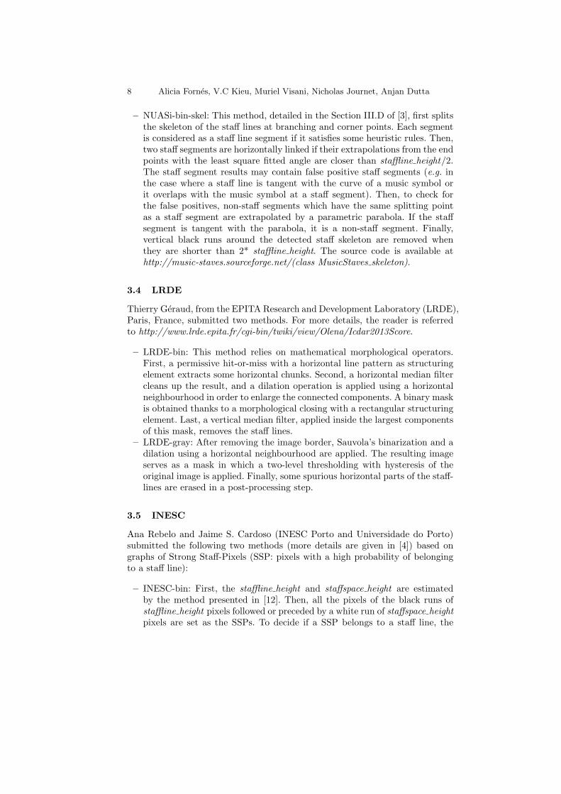
– NUASi-bin-skel: This method, detailed in the Section III.D of [3], first splitsthe skeleton of the staff lines at branching and corner points. Each segmentis considered as a staff line segment if it satisfies some heuristic rules. Then,two staff segments are horizontally linked if their extrapolations from the endpoints with the least square fitted angle are closer than staffline height/2.The staff segment results may contain false positive staff segments (e.g. inthe case where a staff line is tangent with the curve of a music symbol orit overlaps with the music symbol at a staff segment). Then, to check forthe false positives, non-staff segments which have the same splitting pointas a staff segment are extrapolated by a parametric parabola. If the staffsegment is tangent with the parabola, it is a non-staff segment. Finally,vertical black runs around the detected staff skeleton are removed whenthey are shorter than 2* staffline height. The source code is available athttp://music-staves.sourceforge.net/(class MusicStaves skeleton).

3.4 LRDE

Thierry Geraud, from the EPITA Research and Development Laboratory (LRDE),Paris, France, submitted two methods. For more details, the reader is referredto http://www.lrde.epita.fr/cgi-bin/twiki/view/Olena/Icdar2013Score.

– LRDE-bin: This method relies on mathematical morphological operators.First, a permissive hit-or-miss with a horizontal line pattern as structuringelement extracts some horizontal chunks. Second, a horizontal median filtercleans up the result, and a dilation operation is applied using a horizontalneighbourhood in order to enlarge the connected components. A binary maskis obtained thanks to a morphological closing with a rectangular structuringelement. Last, a vertical median filter, applied inside the largest componentsof this mask, removes the staff lines.

– LRDE-gray: After removing the image border, Sauvola’s binarization and adilation using a horizontal neighbourhood are applied. The resulting imageserves as a mask in which a two-level thresholding with hysteresis of theoriginal image is applied. Finally, some spurious horizontal parts of the staff-lines are erased in a post-processing step.

3.5 INESC

Ana Rebelo and Jaime S. Cardoso (INESC Porto and Universidade do Porto)submitted the following two methods (more details are given in [4]) based ongraphs of Strong Staff-Pixels (SSP: pixels with a high probability of belongingto a staff line):

– INESC-bin: First, the staffline height and staffspace height are estimatedby the method presented in [12]. Then, all the pixels of the black runs ofstaffline height pixels followed or preceded by a white run of staffspace heightpixels are set as the SSPs. To decide if a SSP belongs to a staff line, the


image grid is considered as a graph with pixels as nodes, and arcs connectingneighbouring pixels. Then, SSPs are classified as staff line pixels acording tosome heuristic rules. Then, the groups of 5 staff lines are located among theshortest paths by using a global optimization process on the graph.

– INESC-gray: For grayscale images, the weight function is generalized byusing a sigmoid function. The parameters of the sigmoid function are chosento favor the luminance levels of the stafflines. A state-of-the-art binarizationtechnique is used in order to assign the cost for each pixel in the graph(pixels binarized to white have a high cost; pixels binarized to black have alow cost). Once the image is binarized, the previous method is applied.

4 Results

In this section we compare the participant’s output images with the ground-truth (binary staff-less images) of the test set using the measures presented inthe next Section. The ground-truth associated to the test set was made publicafter the competition.

4.1 Measures Used for Performance Comparison

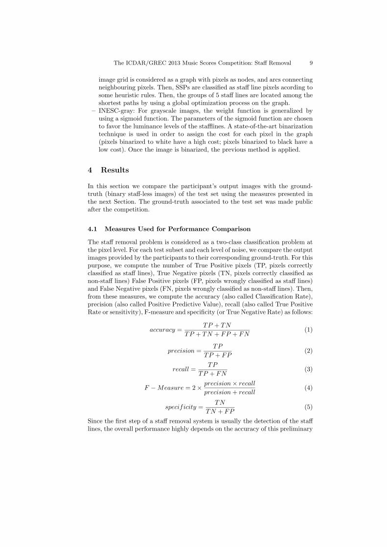
The staff removal problem is considered as a two-class classification problem atthe pixel level. For each test subset and each level of noise, we compare the outputimages provided by the participants to their corresponding ground-truth. For thispurpose, we compute the number of True Positive pixels (TP, pixels correctlyclassified as staff lines), True Negative pixels (TN, pixels correctly classified asnon-staff lines) False Positive pixels (FP, pixels wrongly classified as staff lines)and False Negative pixels (FN, pixels wrongly classified as non-staff lines). Then,from these measures, we compute the accuracy (also called Classification Rate),precision (also called Positive Predictive Value), recall (also called True PositiveRate or sensitivity), F-measure and specificity (or True Negative Rate) as follows:

accuracy =TP + TN

TP + TN + FP + FN(1)

precision =TP

TP + FP(2)

recall =TP

TP + FN(3)

F −Measure = 2×precision× recall

precision+ recall(4)

specificity =TN

TN + FP(5)

Since the first step of a staff removal system is usually the detection of the stafflines, the overall performance highly depends on the accuracy of this preliminary


staff detection. Indeed, if the staff line is undetected, it is unable to be removed.For example, a staff removal system may obtain very good results (when the staffis correctly detected) while rejecting many music scores images (if no staff line isdetected in the image, it is discarded). Therefore, for each participant’s method,we provide the number of rejected pages for each of the three test subsets, andfor each level of degradation inside each test subset. Furthermore, we computethe evaluation measures (1-5) in two ways:

– Without rejection: the five average values of the five measures (1-5) arecomputed inside each test subset and for each level of degradation, takinginto account only the images that the system pre-classified as music score.Thus, the rejected images are not taken into account for these measures.

– With rejection: the five average values of the five measures (1-5) are com-puted inside each test subset and for each level of degradation, taking intoaccount every image in the test set, no matter if it was rejected by the sys-tem or not. Thus, for a rejected image, every staff line pixel is consideredas a False Negative and every non-staff line pixel is considered as a FalsePositive.

4.2 Baseline

For comparison purposes, we have computed some baseline results using theexisting staff removal method proposed by Dutta et al. [13]. This method isbased on the analysis of neighboring components. Basically, it assumes that astaff-line candidate segment is a horizontal linkage of vertical black runs withuniform height. Then, some neighboring properties are used to validate or discardthese segments.

4.3 Performance comparison

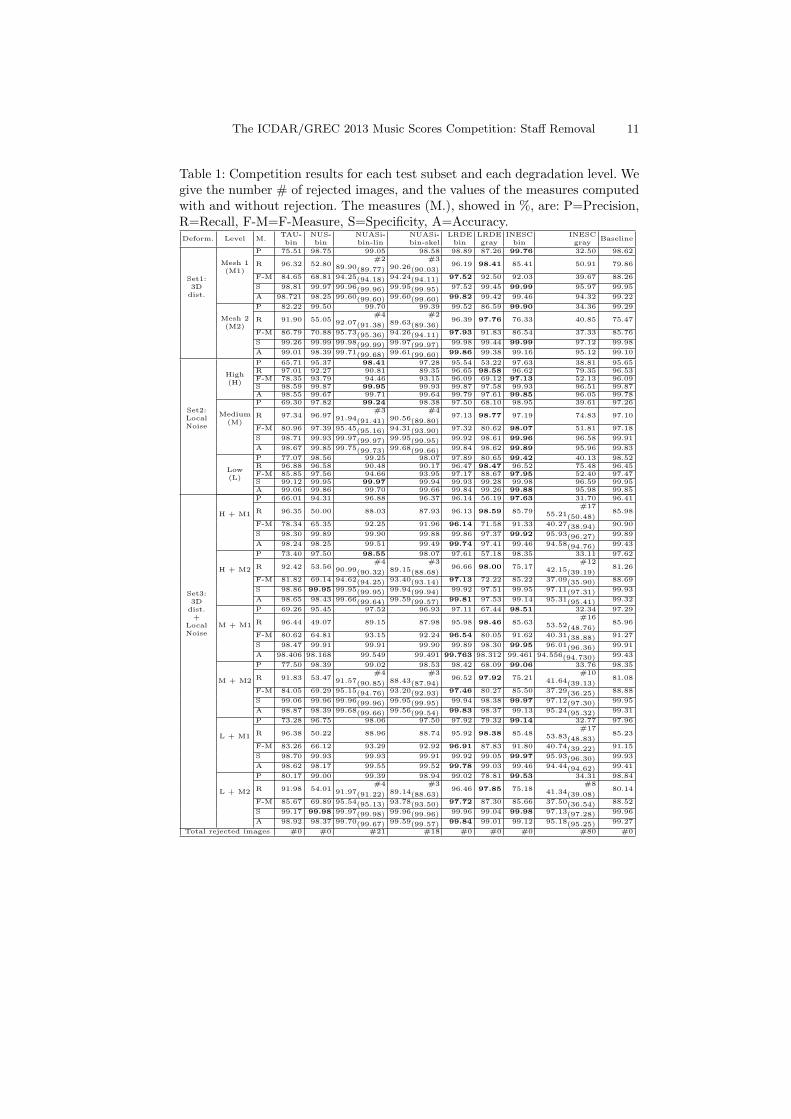
Table 1 and Fig. 7 present staff removal results obtained by the eight participantmethods (three out of the five participants presented two different algorithms).We have also tested the baseline method presented in [13]. Each of the ninecolumns indicates the name of the participant and the staff removal methodcategory. All the metrics used for performance comparison (presented in section4.1) are presented according to the type of degradation (3D distortion, localnoise model, or a mixture of the two) and the degree of degradation. Indeed, foreach sub-dataset five metrics are presented. The winner’s method of each line ishighlighted in bold.

Since the precision is higher in some methods but with a lower recall, wedecided to select the winners according to the accuracy and the F-measure met-rics shown in Fig. 7. From Table 1, we can see that the LRDE-bin method isthe winner of the 3D distortion set, the INESC-bin is the winner of the Localnoise set, and LRDE-bin is the winner of the combination set. Fig. 7 presentsaverages Accuracy and F-Measures of the nine tested methods on three differentsub-datasets (3D distortion, local noise model, a mixture of the two), whereas


Table 1: Competition results for each test subset and each degradation level. Wegive the number # of rejected images, and the values of the measures computedwith and without rejection. The measures (M.), showed in %, are: P=Precision,R=Recall, F-M=F-Measure, S=Specificity, A=Accuracy.Deform. Level M.

TAU-bin

NUS-bin

NUASi-bin-lin

NUASi-bin-skel

LRDEbin

LRDEgray

INESCbin

INESCgray

Baseline

Set1:3Ddist.

Mesh 1(M1)

P 75.51 98.75 99.05 98.58 98.89 87.26 99.76 32.50 98.62

R 96.32 52.80#2

89.90(89.77)

#390.26(90.03)

96.19 98.41 85.41 50.91 79.86

F-M 84.65 68.81 94.25(94.18) 94.24(94.11) 97.52 92.50 92.03 39.67 88.26

S 98.81 99.97 99.96(99.96) 99.95(99.95) 97.52 99.45 99.99 95.97 99.95

A 98.721 98.25 99.60(99.60) 99.60(99.60) 99.82 99.42 99.46 94.32 99.22

Mesh 2(M2)

P 82.22 99.50 99.70 99.39 99.52 86.59 99.90 34.36 99.29

R 91.90 55.05#4

92.07(91.38)

#289.63(89.36)

96.39 97.76 76.33 40.85 75.47

F-M 86.79 70.88 95.73(95.36) 94.26(94.11) 97.93 91.83 86.54 37.33 85.76

S 99.26 99.99 99.98(99.99) 99.97(99.97) 99.98 99.44 99.99 97.12 99.98

A 99.01 98.39 99.71(99.68) 99.61(99.60) 99.86 99.38 99.16 95.12 99.10

Set2:LocalNoise

High(H)

P 65.71 95.37 98.41 97.28 95.54 53.22 97.63 38.81 95.65R 97.01 92.27 90.81 89.35 96.65 98.58 96.62 79.35 96.53F-M 78.35 93.79 94.46 93.15 96.09 69.12 97.13 52.13 96.09S 98.59 99.87 99.95 99.93 99.87 97.58 99.93 96.51 99.87A 98.55 99.67 99.71 99.64 99.79 97.61 99.85 96.05 99.78

Medium(M)

P 69.30 97.82 99.24 98.38 97.50 68.10 98.95 39.61 97.26

R 97.34 96.97#3

91.94(91.41)

#490.56(89.80)

97.13 98.77 97.19 74.83 97.10

F-M 80.96 97.39 95.45(95.16) 94.31(93.90) 97.32 80.62 98.07 51.81 97.18

S 98.71 99.93 99.97(99.97) 99.95(99.95) 99.92 98.61 99.96 96.58 99.91

A 98.67 99.85 99.75(99.73) 99.68(99.66) 99.84 98.62 99.89 95.96 99.83

Low(L)

P 77.07 98.56 99.25 98.07 97.89 80.65 99.42 40.13 98.52R 96.88 96.58 90.48 90.17 96.47 98.47 96.52 75.48 96.45F-M 85.85 97.56 94.66 93.95 97.17 88.67 97.95 52.40 97.47S 99.12 99.95 99.97 99.94 99.93 99.28 99.98 96.59 99.95A 99.06 99.86 99.70 99.66 99.84 99.26 99.88 95.98 99.85

Set3:3Ddist.+

LocalNoise

H + M1

P 66.01 94.31 96.88 96.37 96.14 56.19 97.63 31.70 96.41

R 96.35 50.00 88.03 87.93 96.13 98.59 85.79#17

55.21(50.48)85.98

F-M 78.34 65.35 92.25 91.96 96.14 71.58 91.33 40.27(38.94) 90.90

S 98.30 99.89 99.90 99.88 99.86 97.37 99.92 95.93(96.27) 99.89

A 98.24 98.25 99.51 99.49 99.74 97.41 99.46 94.58(94.76) 99.43

H + M2

P 73.40 97.50 98.55 98.07 97.61 57.18 98.35 33.11 97.62

R 92.42 53.56#4

90.99(90.32)

#389.15(88.68)

96.66 98.00 75.17#12

42.15(39.19)81.26

F-M 81.82 69.14 94.62(94.25) 93.40(93.14) 97.13 72.22 85.22 37.09(35.90) 88.69

S 98.86 99.95 99.95(99.95) 99.94(99.94) 99.92 97.51 99.95 97.11(97.31) 99.93

A 98.65 98.43 99.66(99.64) 99.59(99.57) 99.81 97.53 99.14 95.31(95.41) 99.32

M + M1

P 69.26 95.45 97.52 96.93 97.11 67.44 98.51 32.34 97.29

R 96.44 49.07 89.15 87.98 95.98 98.46 85.63#16

53.52(48.76)85.96

F-M 80.62 64.81 93.15 92.24 96.54 80.05 91.62 40.31(38.88) 91.27

S 98.47 99.91 99.91 99.90 99.89 98.30 99.95 96.01(96.36) 99.91

A 98.406 98.168 99.549 99.491 99.763 98.312 99.461 94.556(94.730) 99.43

M + M2

P 77.50 98.39 99.02 98.53 98.42 68.09 99.06 33.76 98.35

R 91.83 53.47#4

91.57(90.85)

#388.43(87.94)

96.52 97.92 75.21#10

41.64(39.13)81.08

F-M 84.05 69.29 95.15(94.76) 93.20(92.93) 97.46 80.27 85.50 37.29(36.25) 88.88

S 99.06 99.96 99.96(99.96) 99.95(99.95) 99.94 98.38 99.97 97.12(97.30) 99.95

A 98.87 98.39 99.68(99.66) 99.56(99.54) 99.83 98.37 99.13 95.24(95.32) 99.31

L + M1

P 73.28 96.75 98.06 97.50 97.92 79.32 99.14 32.77 97.96

R 96.38 50.22 88.96 88.74 95.92 98.38 85.48#17

53.83(48.83)85.23

F-M 83.26 66.12 93.29 92.92 96.91 87.83 91.80 40.74(39.22) 91.15

S 98.70 99.93 99.93 99.91 99.92 99.05 99.97 95.93(96.30) 99.93

A 98.62 98.17 99.55 99.52 99.78 99.03 99.46 94.44(94.62) 99.41

L + M2

P 80.17 99.00 99.39 98.94 99.02 78.81 99.53 34.31 98.84

R 91.98 54.01#4

91.97(91.22)

#389.14(88.63)

96.46 97.85 75.18#8

41.34(39.08)80.14

F-M 85.67 69.89 95.54(95.13) 93.78(93.50) 97.72 87.30 85.66 37.50(36.54) 88.52

S 99.17 99.98 99.97(99.98) 99.96(99.96) 99.96 99.04 99.98 97.13(97.28) 99.96

A 98.92 98.37 99.70(99.67) 99.59(99.57) 99.84 99.01 99.12 95.18(95.25) 99.27

Total rejected images #0 #0 #21 #18 #0 #0 #0 #80 #0


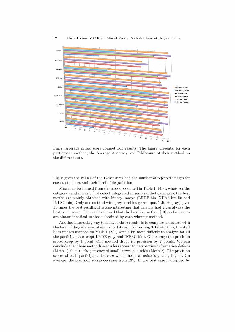
Fig. 7: Average music score competition results. The figure presents, for eachparticipant method, the Average Accuracy and F-Measure of their method onthe different sets.

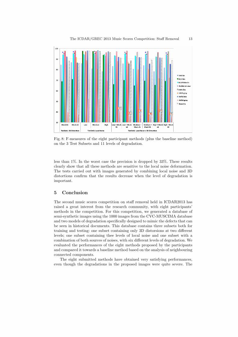
Fig. 8 gives the values of the F-measures and the number of rejected images foreach test subset and each level of degradation.

Much can be learned from the scores presented in Table 1. First, whatever thecategory (and intensity) of defect integrated in semi-synthetics images, the bestresults are mainly obtained with binary images (LRDE-bin, NUAS-bin-lin andINESC-bin). Only one method with grey-level image as input (LRDE-gray) gives11 times the best results. It is also interesting that this method gives always thebest recall score. The results showed that the baseline method [13] performancesare almost identical to those obtained by each winning method.

Another interesting way to analyze these results is to compare the scores withthe level of degradations of each sub dataset. Concerning 3D distortion, the stafflines images mapped on Mesh 1 (M1) were a bit more difficult to analyze for allthe participants (except LRDE-gray and INESC-bin). On average the precisionscores drop by 1 point. One method drops its precision by 7 points. We canconclude that these methods seems less robust to perspective deformation defects(Mesh 1) than to the presence of small curves and folds (Mesh 2). The precisionscores of each participant decrease when the local noise is getting higher. Onaverage, the precision scores decrease from 13%. In the best case it dropped by


Fig. 8: F-measures of the eight participant methods (plus the baseline method)on the 3 Test Subsets and 11 levels of degradation.

less than 1%. In the worst case the precision is dropped by 33%. These resultsclearly show that all these methods are sensitive to the local noise deformation.The tests carried out with images generated by combining local noise and 3Ddistortions confirm that the results decrease when the level of degradation isimportant.

5 Conclusion

The second music scores competition on staff removal held in ICDAR2013 hasraised a great interest from the research community, with eight participants’methods in the competition. For this competition, we generated a database ofsemi-synthetic images using the 1000 images from the CVC-MUSCIMA databaseand two models of degradation specifically designed to mimic the defects that canbe seen in historical documents. This database contains three subsets both fortraining and testing: one subset containing only 3D distorsions at two differentlevels; one subset containing thee levels of local noise and one subset with acombination of both sources of noises, with six different levels of degradation. Weevaluated the performances of the eight methods proposed by the participantsand compared it towards a baseline method based on the analysis of neighbouringconnected components.

The eight submitted methods have obtained very satisfying performances,even though the degradations in the proposed images were quite severe. The


results of the participants have demonstrated that the performance of mostmethods significantly decreases when dealing with a higher level of degrada-tion, especially in the presence of both sources of degradation (3D distortionmodel + local noise model). We hope that our semi-synthetic database, whichis now available on the internet and labelled with different types and levels ofdegradation for both the training set and the test set, will become a benchmarkfor the research on handwritten music scores in the near future.

Acknowledgements

This research was partially funded by the French National Research Agency(ANR) via the DIGIDOC project, and the spanish projects TIN2011-24631 andTIN2012-37475-C02-02.

References

1. D. Blostein and H. S. Baird, Structured Document Image Analysis. SpringerVerlag, 1992, ch. A critical survey of music image analysis, pp. 405–434.

2. A. Rebelo, I. Fujinaga, F. Paszkiewicz, A. Marcal, C. Guedes, and J. Cardoso,“Optical music recognition: state-of-the-art and open issues,” International Journalof Multimedia Information Retrieval, vol. 1, no. 3, pp. 173–190, 2012.

3. C. Dalitz, M. Droettboom, B. Pranzas, and I. Fujinaga, “A comparative study ofstaff removal algorithms,” IEEE Transactions on Pattern Analysis and MachineIntelligence, vol. 30, no. 5, pp. 753–766, 2008.

4. J. dos Santos Cardoso, A. Capela, A. Rebelo, C. Guedes, and J. Pinto da Costa,“Staff detection with stable paths,” IEEE Transactions on Pattern Analysis andMachine Intelligence, vol. 31, no. 6, pp. 1134–1139, 2009.

5. A. Fornes, A. Dutta, A. Gordo, and J. Llados, “The icdar 2011 music scores com-petition: Staff removal and writer identification,” in International Conference onDocument Analysis and Recognition (ICDAR), 2011, pp. 1511–1515.

6. ——, “The 2012 music scores competitions: staff removal and writer identification,”in Graphics Recognition. New Trends and Challenges. Lecture Notes in ComputerScience, Y.-B. Kwon and J.-M. Ogier, Eds. Springer, 2013, vol. 7423, pp. 173–186.

7. ——, “Cvc-muscima: a ground truth of handwritten music score images for writeridentification and staff removal,” International Journal on Document Analysis andRecognition (IJDAR), vol. 15, no. 3, pp. 243–251, 2012.

8. V. Kieu, N. Journet, M. Visani, R. Mullot, and J. Domenger, “Semi-synthetic doc-ument image generation using texture mapping on scanned 3d document shapes,”in 12th International Conference on Document Analysis and Recognition (ICDAR),2013, pp. 489–493.

9. V. Kieu, M. Visani, N. Journet, J. P. Domenger, and R. Mullot, “A characterdegradation model for grayscale ancient document images,” in International Con-ference on Pattern Recognition (ICPR), Tsukuba Science City, Japan, Nov. 2012,pp. 685–688.

10. I. Fujinaga and B. Adviser-Pennycook, Adaptive optical music recognition. McGillUniversity, 1997.


11. B. Su, S. Lu, U. Pal, and C. L. Tan, “An effective staff detection and removaltechnique for musical documents,” in IAPR International Workshop on DocumentAnalysis Systems (DAS), 2012, pp. 160–164.

12. J. Cardoso and A. Rebelo, “Robust staffline thickness and distance estimation inbinary and gray-level music scores,” in 20th International Conference on PatternRecognition (ICPR), 2010, pp. 1856–1859.

13. A. Dutta, U. Pal, A. Fornes, and J. Llados, “An efficient staff removal approachfrom printed musical documents,” International Conference on Pattern Recognition(ICPR), pp. 1965–1968, 2010.

the icdar/grec 2013 music scores competition: staff removal

Documents