HAL Id: hal-03256193https://hal.archives-ouvertes.fr/hal-03256193

Submitted on 10 Jun 2021

HAL is a multi-disciplinary open accessarchive for the deposit and dissemination of sci-entific research documents, whether they are pub-lished or not. The documents may come fromteaching and research institutions in France orabroad, or from public or private research centers.

L’archive ouverte pluridisciplinaire HAL, estdestinée au dépôt et à la diffusion de documentsscientifiques de niveau recherche, publiés ou non,émanant des établissements d’enseignement et derecherche français ou étrangers, des laboratoirespublics ou privés.

ICDAR 2021 Competition on Historical MapSegmentation

Joseph Chazalon, Edwin Carlinet, Yizi Chen, Julien Perret, BertrandDuménieu, Clément Mallet, Thierry Géraud, Vincent Nguyen, Nam Nguyen,

Josef Baloun, et al.

To cite this version:Joseph Chazalon, Edwin Carlinet, Yizi Chen, Julien Perret, Bertrand Duménieu, et al.. ICDAR 2021Competition on Historical Map Segmentation. 16th International Conference on Document Analysisand Recognition (ICDAR’21), Sep 2021, Lausanne, Switzerland. pp.693-707, �10.1007/978-3-030-86337-1_46�. �hal-03256193�

ICDAR 2021 Competition onHistorical Map Segmentation?

Joseph Chazalon1 , Edwin Carlinet1 , Yizi Chen1,2 , Julien Perret2,3 ,Bertrand Dumenieu3 , Clement Mallet2 , Thierry Geraud1 ,

Vincent Nguyen4,5 , Nam Nguyen4,Josef Baloun6,7 , Ladislav Lenc6,7 , and Pavel Kral6,7

1 EPITA Research and Development Lab. (LRDE), EPITA, France2 Univ. Gustave Eiffel, IGN-ENSG, LaSTIG, France

3 LaDeHiS, CRH, EHESS, France4 L3i, University of La Rochelle, France

5 Liris, INSA-Lyon, France6 Department of Computer Science and Engineering, University of West Bohemia,

Univerzitnı, Pilsen, Czech Republic7 NTIS - New Technologies for the Information Society, University of West Bohemia,

Univerzitnı, Pilsen, Czech Republic

Abstract. This paper presents the final results of the ICDAR 2021Competition on Historical Map Segmentation (MapSeg), encouraging re-search on a series of historical atlases of Paris, France, drawn at 1/5000scale between 1894 and 1937. The competition featured three tasks,awarded separately. Task 1 consists in detecting building blocks and waswon by the L3IRIS team using a DenseNet-121 network trained in aweakly supervised fashion. This task is evaluated on 3 large images con-taining hundreds of shapes to detect. Task 2 consists in segmenting mapcontent from the larger map sheet, and was won by the UWB team us-ing a U-Net-like FCN combined with a binarization method to increasedetection edge accuracy. Task 3 consists in locating intersection pointsof geo-referencing lines, and was also won by the UWB team who useda dedicated pipeline combining binarization, line detection with Houghtransform, candidate filtering, and template matching for intersectionrefinement. Tasks 2 and 3 are evaluated on 95 map sheets with com-plex content. Dataset, evaluation tools and results are available underpermissive licensing at https://icdar21-mapseg.github.io/.

Keywords: Historical Maps · Map Vectorization · Competition

1 Introduction

Motivation This competition consists in solving several challenges which ariseduring the processing of images of historical maps. In the Western world, the

? This work was partially funded by the French National Research Agency (ANR):Project SoDuCo, grant ANR-18-CE38-0013. We thank the City of Paris for grantingus with the permission to use and reproduce the atlases used in this work.

2 J. Chazalon et al.

Fig. 1: Sample map sheet. Original size: 11136×7711 pixels.

Fig. 2: Some map-related challenges (left): visual polysemy, planimetric overlap,text overlap. . . and some document-related challenges (right): damaged paper,non-straight lines, image compression, handwritten text. . .

rapid development of geodesy and cartography from the 18th century resultedin massive production of topographic maps at various scales. City maps are ofutter interest. They contain rich, detailed, and often geometrically accurate rep-resentations of numerous geographical entities. Recovering spatial and semanticinformation represented in old maps requires a so-called vectorization process.Vectorizing maps consists in transforming rasterized graphical representations ofgeographic entities (often maps) into instanced geographic data (or vector data),that can be subsequently manipulated (using Geographic Information Systems).This is a key challenge today to better preserve, analyze and disseminate contentfor numerous spatial and spatio-temporal analysis purposes.

Tasks From a document analysis and recognition (DAR) perspective, fullmap vectorization covers a wide range of challenges, from content separation totext recognition. MapSeg focuses on 3 critical steps of this process. (i) Hierarchi-

ICDAR’21 MapSeg 3

cal information extraction, and more specifically the detection of building blockswhich form a core layer of map content. This is addressed in Task 1. (ii) Mapcontent segmentation, which needs to be performed very early in the processingpipeline to separate meta-data like titles, legends and other elements from coremap content. This is addressed in Task 2. (iii) Geo-referencing, i.e. mapping his-torical coordinate system into a recent reference coordinate system. Automatingthis process requires the detection of well-referenced points, and we are partic-ularly interested in detecting intersection points between graticule lines for thispurpose. This is addressed in Task 3.

Dataset MapSeg dataset is extracted from a series of 9 atlases of the City ofParis8 produced between 1894 and 1937 by the Map Service (“Service du plan”)of the City of Paris, France, for the purpose of urban management and planning.For each year, a set of approximately 20 sheets forms a tiled view of the city,drawn at 1/5000 scale using trigonometric triangulation. Figure 1 is an exampleof such sheet. Such maps are highly detailed and very accurate even by modernstandards. This material provides a very valuable resource for historians anda rich body of scientific challenges for the document analysis and recognition(DAR) community: map-related challenges (fig. 2, left) and document-relatedones (fig. 2, right). The actual dataset is built from a selection of 132 map sheetsextracted from these atlases. Annotation was performed manually by trainedannotators and required 400 hours of manual work to annotate the 5 sheets ofthe dataset for Task 1 and 100 hours to annotate the 127 sheets for Tasks 2and 3. A special care was observed to minimize the spatial and, to some extent,temporal overlap between train, validation and test sets: except for Task 1 whichcontains districts 1 and 2 both in train and test sets (from different atlases toassess the potential for the exploitation of information redundancy over time),each district is either in the training, the validation or the test set. This isparticularly important for Tasks 2 and 3 as the general organization of the mapsheets are very similar for sheets representing the same area.

Competition Protocol The MapSeg challenge ran from November 2020 toApril 2021. Participants were provided with training and validation sets for each3 tasks by November 2020. The test phase for Task 1 started with the release oftest data on April 5th, 2021 and ended in April 9th. The test phase for Tasks 2and 3 started with the release of test data on April 12th, 2021 and ended inApril 16th. Participants were requested to submit the results produced by theirmethods (at most 2) over the test images, computed by themselves.

Open Data, Tools and Results To improve the reliability of the evalu-ation and competition transparency, evaluation tools were released (executableand open source code) early in the competition, so participants were able toevaluate their methods on the validation set using exactly the same tools asthe organizers on the test set. More generally, all competition material is made

8 Atlas municipal des vingt arrondissements de Paris. 1894, 1895, 1898, 1905, 1909,1912, 1925, 1929, and 1937. Bibliotheque de l’Hotel de Ville. City of Paris. France.Online resources for the 1925 atlas: https://bibliotheques-specialisees.paris.fr/ark:/73873/pf0000935524.

4 J. Chazalon et al.

available under very permissive licenses at https://icdar21-mapseg.github.io/:dataset with ground truth, evaluation tools and participants results can be down-loaded, inspected, copied and modified.

Participants The following teams took part in the competition.

CMM Team: Team: Mateus Sangalli, Beatriz Marcotegui, Jose Marcio Mar-tins Da Cruz, Santiago Velasco-Forero, Samy Blusseau; Institutions: Cen-ter for Mathematical Morphology, Mines ParisTech, PSL Research Univer-sity, France; Extra material: morphological library Smil: http://smil.cmm.minesparis.psl.eu; code: https://github.com/MinesParis-MorphoMath.

IRISA Team: Competitor: Aurelie Lemaitre; Institutions: IRISA/UniversiteRennes 2, Rennes, France; Extra material: http://www.irisa.fr/intuidoc/.

L3IRIS Team: Team: Vincent Nguyen and Nam Nguyen; Institutions: L3i,University of La Rochelle, France; Liris, INSA-Lyon, France; Extra material:https://gitlab.univ-lr.fr/nnguye02/weakbiseg.

UWB Team: Team: Josef Baloun, Ladislav Lenc and Pavel Kral; Institutions:Department of Computer Science and Engineering, University of West Bo-hemia, Univerzitnı, Pilsen, Czech Republic; NTIS - New Technologies forthe Information Society, University of West Bohemia, Univerzitnı, Pilsen,Czech Republic; Extra material: https://gitlab.kiv.zcu.cz/balounj/21 icdarmapseg competition.

WWU Team: Team: Sufian Zaabalawi, Benjamin Risse; Institution: MunsterUniversity, Germany; Extra material: Project on automatic vectorization ofhistorical cadastral maps: https://dhistory.hypotheses.org/346.

2 Task 1: Detect Building Blocks

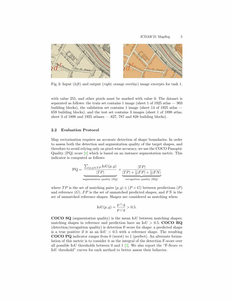
This task consists in detecting a set of closed shapes (building blocks) in themap image. Building blocks are coarser map objects which can regroup severalelements. Detecting these objects is a critical step in the digitization of historicalmaps because it provides essential components of a city. Each building block issymbolized by a closed shape which can enclose other objects and lines. Buildingblocks are surrounded by streets, rivers fortification wall or others, and are neverdirectly connected. Building blocks can sometimes be reduced to a single spacialbuilding, symbolized by diagonal hatched areas. Given the image of a completemap sheet and a mask of the map area, participants had to detect each buildingblock as illustrated in fig. 3.

2.1 Dataset

Inputs form a set of JPEG RGB images which are quite large (≈ 8000 × 8000pixels). They are complete map sheet images as illustrated in fig. 1, cropped tothe relevant area (using the ground truth from Task 2). Remaining non-relevantpixels were replaced by black pixels. Expected output for this task is a binarymask of the building blocks: pixels falling inside a building block must be marked

ICDAR’21 MapSeg 5

Fig. 3: Input (left) and output (right, orange overlay) image excerpts for task 1.

with value 255, and other pixels must be marked with value 0. The dataset isseparated as follows: the train set contains 1 image (sheet 1 of 1925 atlas — 903building blocks), the validation set contains 1 image (sheet 14 of 1925 atlas —659 building blocks), and the test set contains 3 images (sheet 1 of 1898 atlas,sheet 3 of 1898 and 1925 atlases — 827, 787 and 828 building blocks).

2.2 Evaluation Protocol

Map vectorization requires an accurate detection of shape boundaries. In orderto assess both the detection and segmentation quality of the target shapes, andtherefore to avoid relying only on pixel-wise accuracy, we use the COCO PanopticQuality (PQ) score [8] which is based on an instance segmentation metric. Thisindicator is computed as follows:

PQ =

∑(p,g)∈TP IoU(p, g)

|TP |︸ ︷︷ ︸segmentation quality (SQ)

× |TP ||TP |+ 1

2 |FP |+12 |FN |︸ ︷︷ ︸

recognition quality (RQ)

where TP is the set of matching pairs (p, g) ∈ (P ×G) between predictions (P )and reference (G), FP is the set of unmatched predicted shapes, and FN is theset of unmatched reference shapes. Shapes are considered as matching when:

IoU(p, g) =p ∩ gp ∪ g

> 0.5.

COCO SQ (segmentation quality) is the mean IoU between matching shapes:matching shapes in reference and prediction have an IoU > 0.5. COCO RQ(detection/recognition quality) is detection F-score for shape: a predicted shapeis a true positive if it as an IoU > 0.5 with a reference shape. The resultingCOCO PQ indicator ranges from 0 (worst) to 1 (perfect). An alternate formu-lation of this metric is to consider it as the integral of the detection F-score overall possible IoU thresholds between 0 and 1 [4]. We also report the “F-Score vsIoU threshold” curves for each method to better assess their behavior.

6 J. Chazalon et al.

2.3 Method descriptions

L3IRIS — Winning Method From previous experiments, the L3IRIS teamreports that both semantic segmentation and instance segmentation approachesled to moderate results, mainly because of the amount of available data. In-stead of trying to detect building blocks directly, they reversed the problem andtried to detect non-building-blocks as a binary semantic segmentation problemwhich facilitated the training process. Additionally, they considered the prob-lem in a semi/weakly supervised setting where training data includes 2 images(val+train): the label is available for one image and is missing for the other im-age. Their binary segmentation model relies on a DenseNet-121 [7] backbone andis trained using the weakly supervised learning method from [12]. Input is pro-cessed as 480×480 tiles. During training, tiles are generated by random cropsand augmented with standard perturbations: noise, rotation, gray, scale, etc.Some post-processing techniques like morphological operators are used to refinethe final mask (open the lightly connected blocks and fill holes). The parameterfor the post-processing step is selected based on the results on the validationimage. Training output is a single models; not ensemble technique is used. Theweakly supervised training enables the training of a segmentation network in asetting where only a subset of the training objects are labelled. The overcomethe problem of missing labels, the L3IRIS team uses two energy maps w+ et w−which represent the certainty that a pixel being positive (object’s pixel) or nega-tive (background pixel). These two energy maps are evolved during the trainingat each epoch based on prediction scores in multiple past epochs. This techniqueimplicitly minimizes the entropy of the predictions on unlabeled data which canhelp to boost the performance of the model [5]. For Task 1, they consideredlabeled images (from training set) and unlabeled ones (from validation set) forwhich the label was retained for validation. The two energy maps are appliedonly for images from the validation set.

CMM Method 1 This method combines two parallel sub-methods, named 1Aand 1B. In both sub-methods, the RGB images are first processed by a U-Net [14]trained to find edges of the blocks. Then, a morphological processing is applied tothe image of edges in order to segment the building blocks. Finally, the results ofboth sub-methods are combined to produce a unique output. In method 1A, theU-Net is trained with data augmentation that uses random rotations, reflections,occlusion by vertical and horizontal lines and color changes. The loss functionpenalizes possible false positive pixels (chosen based on the distance from edgepixels in the color space) with a higher cost. To segment the blocks, first atop-hat operator is applied to remove large vertical and horizontal lines and ananisotropic closing [3] is used to remove holes in the edges. Edges are binarizedby a hysteresis threshold and building blocks are obtained by a fill-holes operatorfollowed by some post-processing. The result is a clean segmentation, but withsome relatively large empty regions. In method 1B, the U-Net is trained using thesame augmentation process, but the loss function weights errors to compensateclass imbalance. Method 2 (described hereafter) is applied to the inverse of the

ICDAR’21 MapSeg 7

edges obtained by this second U-Net. To combine both methods, a closing by alarge structuring element is used to find the dense regions in the output of 1A,the complement of which are the empty regions of 1A. The final output is equalto 1A in the dense region and to 1B in the empty regions.

Method 2 This method is fully morphological. It works on a gray-levelimage, obtained by computing the luminance from the RGB color image. Themain steps are the following: (i) Area closing with 1000 pixels as area threshold;this step aims at removing small dark components such as letters. (ii) Inversionof contrast of the resulting image followed by a fill-holes operator; The resultof this step is an image where most blocks appear as flat zones, and so dolarge portions of streets. (iii) The morphological gradient of the previous imageis computed and then reconstructed by erosion starting from markers chosenas the minima with dynamic not smaller than h = 2. This produces a new,simplified, gradient image. (iv) The watershed transform is applied to the latterimage, yielding a labelled image. (v) A filtering of labelled components removes(that is, sets to zero) components smaller than 2000 pixels and larger than 1Mpixels; and also removes the components with area smaller than 0.3 times thearea of their bounding box (this removes large star-shaped street components).All kept components are set to 255 to produce a binary image. (vi) A fill-holesoperator is applied to the latter binary image. (vii) Removal of river components:A mask of the river is computed by a morphological algorithm based on a largeopening followed by a much larger closing, a threshold and further refinements.Components with an intersection of at least 60% of their area with the rivermask are removed.

WWU Method 1 This method relies on a binary semantic segmentation U-Net [14] trained with Dice loss on a manual selection of 2000 image patchesof size 256×256×3 covering representative map areas. The binary segmentationground truth is directly used as target. This U-Net architecture uses 5 blocks andeach convolutional layer has a 3×3 kernel filter with no padding. The expendingpath uses transpose convolutions with 2× stride. Intermediate activations useRELU and the final activation is a sigmoid.

Method 2 This method relies on a Deep Distance transform. The binarylabel image is first transformed into a Euclidean distance transform map (DTM),which highlights the inner region of the building blocks more than the outeredges. Like for method 1, 2000 training patch pairs of size 256×256 are generated.The U-Net architecture is similar to the previous method, except that the lossfunction is the mean square error loss (MSE) and the prediction is a DTM. ThisDTM is then thresholded and a watershed transform is used to fill regions ofinterest and extract building block shapes.

2.4 Results and discussion

Results and ranking of each submitted method is given in fig. 4: table on the leftsummarizes the COCO PQ indicators we computed and the plot on the right

8 J. Chazalon et al.

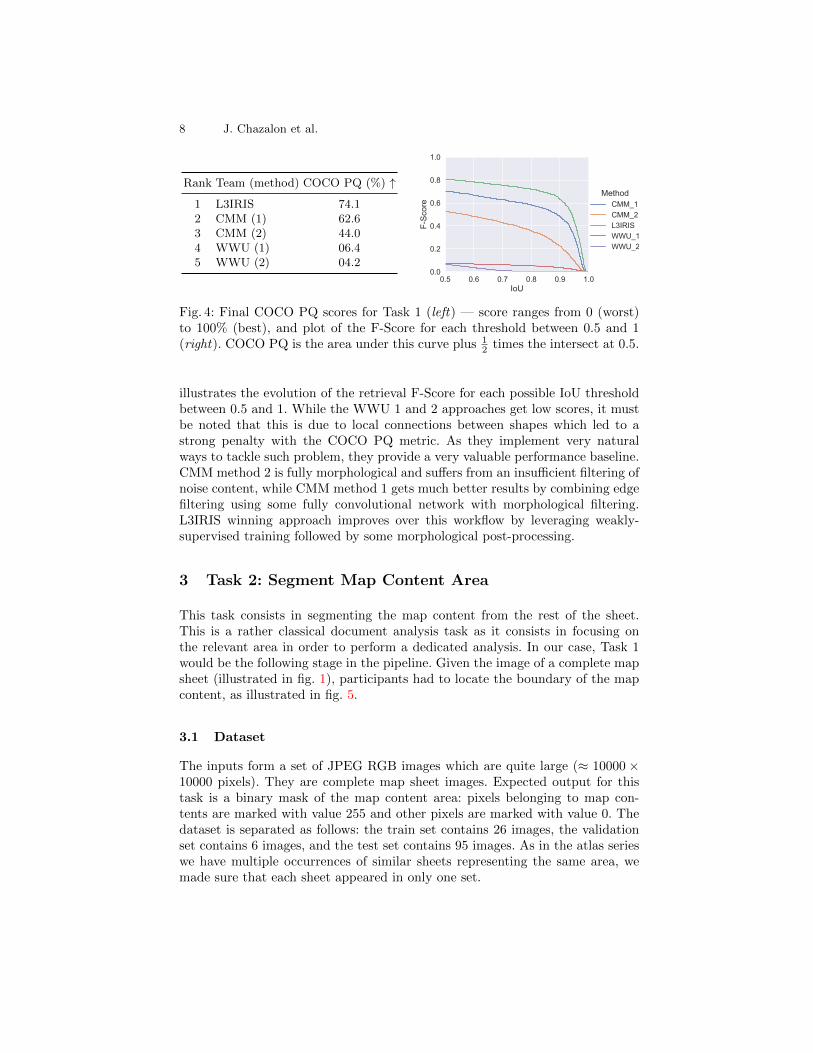
Rank Team (method) COCO PQ (%) ↑

1 L3IRIS 74.12 CMM (1) 62.63 CMM (2) 44.04 WWU (1) 06.45 WWU (2) 04.2

0.5 0.6 0.7 0.8 0.9 1.0IoU

0.0

0.2

0.4

0.6

0.8

1.0

F-Sc

ore

MethodCMM_1CMM_2L3IRISWWU_1WWU_2

Fig. 4: Final COCO PQ scores for Task 1 (left) — score ranges from 0 (worst)to 100% (best), and plot of the F-Score for each threshold between 0.5 and 1(right). COCO PQ is the area under this curve plus 1

2 times the intersect at 0.5.

illustrates the evolution of the retrieval F-Score for each possible IoU thresholdbetween 0.5 and 1. While the WWU 1 and 2 approaches get low scores, it mustbe noted that this is due to local connections between shapes which led to astrong penalty with the COCO PQ metric. As they implement very naturalways to tackle such problem, they provide a very valuable performance baseline.CMM method 2 is fully morphological and suffers from an insufficient filtering ofnoise content, while CMM method 1 gets much better results by combining edgefiltering using some fully convolutional network with morphological filtering.L3IRIS winning approach improves over this workflow by leveraging weakly-supervised training followed by some morphological post-processing.

3 Task 2: Segment Map Content Area

This task consists in segmenting the map content from the rest of the sheet.This is a rather classical document analysis task as it consists in focusing onthe relevant area in order to perform a dedicated analysis. In our case, Task 1would be the following stage in the pipeline. Given the image of a complete mapsheet (illustrated in fig. 1), participants had to locate the boundary of the mapcontent, as illustrated in fig. 5.

3.1 Dataset

The inputs form a set of JPEG RGB images which are quite large (≈ 10000 ×10000 pixels). They are complete map sheet images. Expected output for thistask is a binary mask of the map content area: pixels belonging to map con-tents are marked with value 255 and other pixels are marked with value 0. Thedataset is separated as follows: the train set contains 26 images, the validationset contains 6 images, and the test set contains 95 images. As in the atlas serieswe have multiple occurrences of similar sheets representing the same area, wemade sure that each sheet appeared in only one set.

ICDAR’21 MapSeg 9

Fig. 5: Illustration of expected outputs for Task 2: green area is the map contentand red hatched area is the background.

3.2 Evaluation Protocol

We evaluated the quality of the segmentation using the Hausdorff distance be-tween the ground-truth shape and the predicted one. This measure has theadvantage over the IoU, Jaccard index and other area measures that it keeps agood “contrast” between results in the case of large objects (because there is nonormalization by the area). More specifically, we use the “Hausdorff 95” variantwhich discards the 5 percentiles of higher values (assumed to be outliers) toproduce a more stable measure. Finally, we averaged indicators for all individualmap images to produce a global indicator. The resulting measure is an errormeasure which ranges from 0 (best) to a large value depending on image size.

3.3 Method descriptions

UWB — Winning Method This method is based on the U-Net-like fullyconvolutional networked used in [1]. This network takes a whole downsampledpage as an input and predicts the border of the expected area. Border trainingsamples were generated from the original ground truth (GT) files. The valuesare computed using a Gaussian function, where σ = 50 and the distance fromborder is used. Training is performed using the training set and augmentation(mirroring, rotation and random distortion) [2] to increase the amount of thetraining samples. To improve the location of the detected border, a binarized im-age is generated using a recursive Otsu filter [13] followed by the removal of smallcomponents. Network prediction and the binarized image are post-processed andcombined with the use of connected components and morphological operations,which parameters are calibrated on the validation set. The result of the processis the predicted mask of a map content area.

10 J. Chazalon et al.

CMM This method assumes that the area of interest is characterized by thepresence of black lines connected to each other all over the map. These con-nections being due either to the external frame, graticule lines, streets, or textsuperimposed to the map. Thus, the main idea is detecting black lines and re-constructing them from a predefined rectangle marker in the center of the image.The method is implemented with the following steps. (i) Eliminate map margin(M) detected by the quasi-flat zone algorithm and removed from the whole im-age (I0): I = I0 −M . (ii) Then, black lines (B), are extracted by a thresholdedblack-top-hat (B = Otsu(I−ϕ(I))) (iii) A white rectangle (R) is drawn centeredin the middle of the image and of dimensions W

2 ×H2 , with W and H the image

width and height respectively. (iv) Black lines B are reconstructed by dilationfrom the centered rectangle: Bs = Build(R,B). Several dark frames surroundthe map. Only the inner one is connected to the drawn rectangle R and delimitsthe area of interest. (v) The frame (black line surrounding the map) may not becomplete due to lack of contrast or noise. A watershed is applied to the inverse ofthe distance function in order to close the contour with markers = R ∪ border.The region corresponding to marker R becomes the area of interest. (vi) Finally,legends are removed from the area of interest. Legends are the regions from theinverse of Bs that are rectangular and close to the border of the area of interest.

IRISA This approach is entirely based on a grammatical rule-based system [9]which combines visual clues of line segments extracted in the document at vari-ous levels of a spatial pyramid. The line segment extractor, based on a multi-scaleKalman filtering [10], is fast and robust to noise, and can deal with slope andcurvature. Border detection is performed in two steps: (i) Line segments arefirst extracted at low resolution level (scale 1:16) to provides visual clues on thepresence of the double rulings outside the map region. Then, the coarse enclos-ing rectangle is detected using a set of grammar rules. (ii) Line segments areextracted at medium resolution level (scale 1:2) to detect parts of contours ofthe maps, and of title regions. Another set of grammar rules are then used todescribe and detect the rectangular contour with smaller rectangle (title andlegend) in the corners. The performance is this approach is limited by the gram-mar rules which do not consider, though it would be possible, the fact that themap content may lay outside the rectangular region, nor it considers that somelegend components may not be located at the corners of the map.

L3IRIS This approach leverages the cutting edge few-shot learning techniqueHSNet [11] for image segmentation, in order to cope with the limited amountof training data. With this architecture, the prediction of a new image (queryimage) will be based on the trained model and a training image (support image).In practice, the L3IRIS team trained the HSNet [11] from scratch with a Resnet50 backbone from available data to predict the content area in the input mapwith 512×512 image input. Because post-processing techniques to smooth andfill edges did not improve the evaluation error, the authors kept the results fromthe single trained model as the final predicted maps.

ICDAR’21 MapSeg 11

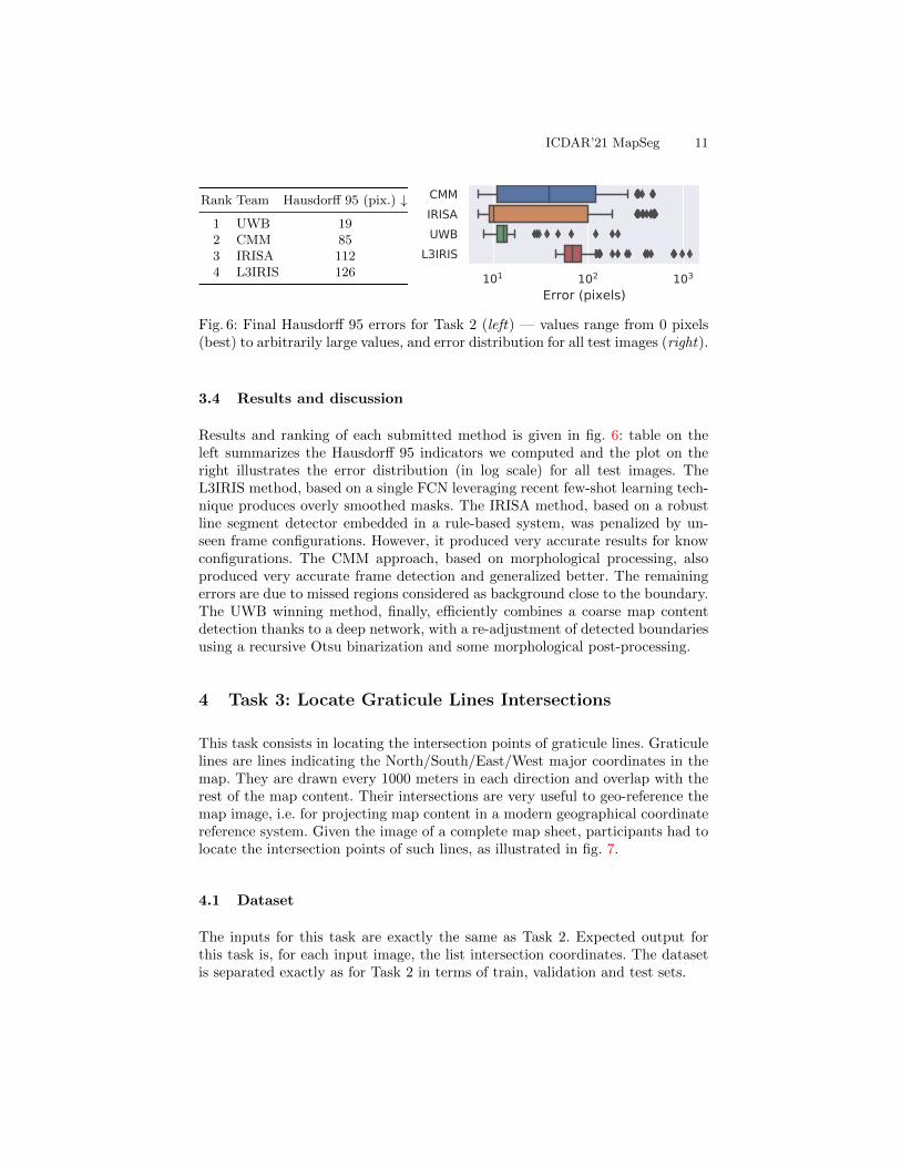
Rank Team Hausdorff 95 (pix.) ↓

1 UWB 192 CMM 853 IRISA 1124 L3IRIS 126 101 102 103

Error (pixels)

CMMIRISAUWB

L3IRIS

Fig. 6: Final Hausdorff 95 errors for Task 2 (left) — values range from 0 pixels(best) to arbitrarily large values, and error distribution for all test images (right).

3.4 Results and discussion

Results and ranking of each submitted method is given in fig. 6: table on theleft summarizes the Hausdorff 95 indicators we computed and the plot on theright illustrates the error distribution (in log scale) for all test images. TheL3IRIS method, based on a single FCN leveraging recent few-shot learning tech-nique produces overly smoothed masks. The IRISA method, based on a robustline segment detector embedded in a rule-based system, was penalized by un-seen frame configurations. However, it produced very accurate results for knowconfigurations. The CMM approach, based on morphological processing, alsoproduced very accurate frame detection and generalized better. The remainingerrors are due to missed regions considered as background close to the boundary.The UWB winning method, finally, efficiently combines a coarse map contentdetection thanks to a deep network, with a re-adjustment of detected boundariesusing a recursive Otsu binarization and some morphological post-processing.

4 Task 3: Locate Graticule Lines Intersections

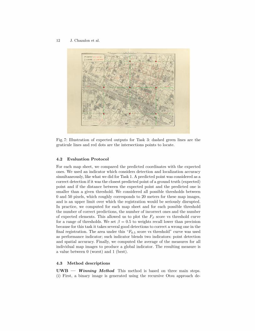
This task consists in locating the intersection points of graticule lines. Graticulelines are lines indicating the North/South/East/West major coordinates in themap. They are drawn every 1000 meters in each direction and overlap with therest of the map content. Their intersections are very useful to geo-reference themap image, i.e. for projecting map content in a modern geographical coordinatereference system. Given the image of a complete map sheet, participants had tolocate the intersection points of such lines, as illustrated in fig. 7.

4.1 Dataset

The inputs for this task are exactly the same as Task 2. Expected output forthis task is, for each input image, the list intersection coordinates. The datasetis separated exactly as for Task 2 in terms of train, validation and test sets.

12 J. Chazalon et al.

Fig. 7: Illustration of expected outputs for Task 3: dashed green lines are thegraticule lines and red dots are the intersections points to locate.

4.2 Evaluation Protocol

For each map sheet, we compared the predicted coordinates with the expectedones. We used an indicator which considers detection and localization accuracysimultaneously, like what we did for Task 1. A predicted point was considered as acorrect detection if it was the closest predicted point of a ground truth (expected)point and if the distance between the expected point and the predicted one issmaller than a given threshold. We considered all possible thresholds between0 and 50 pixels, which roughly corresponds to 20 meters for these map images,and is an upper limit over which the registration would be seriously disrupted.In practice, we computed for each map sheet and for each possible thresholdthe number of correct predictions, the number of incorrect ones and the numberof expected elements. This allowed us to plot the Fβ score vs threshold curvefor a range of thresholds. We set β = 0.5 to weights recall lower than precisionbecause for this task it takes several good detections to correct a wrong one in thefinal registration. The area under this “F0.5 score vs threshold” curve was usedas performance indicator; such indicator blends two indicators: point detectionand spatial accuracy. Finally, we computed the average of the measures for allindividual map images to produce a global indicator. The resulting measure isa value between 0 (worst) and 1 (best).

4.3 Method descriptions

UWB — Winning Method This method is based on three main steps.(i) First, a binary image is generated using the recursive Otsu approach de-

ICDAR’21 MapSeg 13

scribed in section 3.3. This image is then masked using the map content areapredicted for Task 2. (ii) Graticule lines are then detected a Hough Line Trans-form. While the accumulator bins contain a lot of noise, the following heuristicswere used to filter the candidates: graticule lines are assumed to be straight,to be equally spaced and either parallel or perpendicular, and there should beat least four lines in each image. To enable finding, filtering, correcting, fixingand rating peak groups that represents each graticule line in Hough accumu-lator, each candidate contains information about its rating, angle and distancebetween lines. Rating and distance information is used to select the best config-uration. (iii) Intersections are finally coarsely estimated from the intersectionsbetween Hough lines, then corrected and filtered using the predicted mask fromthe Task 2, using some template matching with a cross rotated by the corre-sponding angle. The approach does not require any learning and the parametersare calibrated using both train and validation subsets.

IRISA This method is based on two main steps. (i) The same line segmentdetector as the one used by the IRISA team for Task 2 (section 3.3) is used todetect candidates. This results in a large amount of false positives with segmentsdetected in many map objects. (ii) The DMOS rule grammar system [9] is usedto efficiently filter candidates using a dedicated set of rules. Such rules enablethe integration of constraints like perpendicularity or regular spacing betweenthe lines, and the exploration of the hypothesis space thanks to the efficientback-tracking of the underlying logical programming framework.

CMM This method combines morphological processing and the Radon trans-form. Morphological operators can be disturbed by noise disconnecting long lineswhile the Radon transform can integrate the contribution of short segments thatmay correspond to a fine texture. The process consists in the following six steps.(i) First, the image is sub-sampled by a factor 10 in order to speed up the processand to make it more robust to potential line discontinuities. An erosion of size10 is applied before sub-sampling to preserve black lines. (ii) Then the frameis detected. Oriented gradients combined with morphological filters are used forthis purpose, inspired by the method proposed in [6] for building facade analysis.(iii) Line directions are then found. Directional closings from 0 to 30 degrees witha step of 1 degree, followed by black top-hat and Otsu threshold are applied. Theangle leading to the longest detected line is selected. (iv) The Radon transformof the previous black top-hat at the selected direction and its orthogonal arecomputed. Line locations correspond to the maxima of the Radon transform.(v) Lines are equally spaced in the map. The period of this grid is obtained asthe maximum of the autocorrelation of the Radon transform. Equidistant linesare added on the whole map, whether they have been detected by the Radontransform or not. Applied to both directions, this generates the graticule lines.(vi) Finally a refinement is applied to localize precisely the line intersections atthe full scale. In the neighborhood of each detected intersection, a closing is ap-plied with a cross structuring element (with lines of length 20) at the previously

14 J. Chazalon et al.

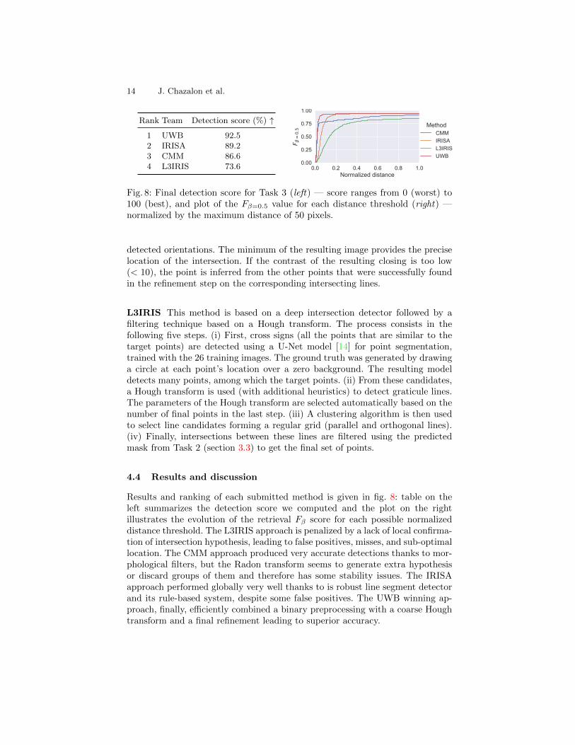
Rank Team Detection score (%) ↑

1 UWB 92.52 IRISA 89.23 CMM 86.64 L3IRIS 73.6 0.0 0.2 0.4 0.6 0.8 1.0

Normalized distance

0.00

0.25

0.50

0.75

1.00

F=

0.5 Method

CMMIRISAL3IRISUWB

Fig. 8: Final detection score for Task 3 (left) — score ranges from 0 (worst) to100 (best), and plot of the Fβ=0.5 value for each distance threshold (right) —normalized by the maximum distance of 50 pixels.

detected orientations. The minimum of the resulting image provides the preciselocation of the intersection. If the contrast of the resulting closing is too low(< 10), the point is inferred from the other points that were successfully foundin the refinement step on the corresponding intersecting lines.

L3IRIS This method is based on a deep intersection detector followed by afiltering technique based on a Hough transform. The process consists in thefollowing five steps. (i) First, cross signs (all the points that are similar to thetarget points) are detected using a U-Net model [14] for point segmentation,trained with the 26 training images. The ground truth was generated by drawinga circle at each point’s location over a zero background. The resulting modeldetects many points, among which the target points. (ii) From these candidates,a Hough transform is used (with additional heuristics) to detect graticule lines.The parameters of the Hough transform are selected automatically based on thenumber of final points in the last step. (iii) A clustering algorithm is then usedto select line candidates forming a regular grid (parallel and orthogonal lines).(iv) Finally, intersections between these lines are filtered using the predictedmask from Task 2 (section 3.3) to get the final set of points.

4.4 Results and discussion

Results and ranking of each submitted method is given in fig. 8: table on theleft summarizes the detection score we computed and the plot on the rightillustrates the evolution of the retrieval Fβ score for each possible normalizeddistance threshold. The L3IRIS approach is penalized by a lack of local confirma-tion of intersection hypothesis, leading to false positives, misses, and sub-optimallocation. The CMM approach produced very accurate detections thanks to mor-phological filters, but the Radon transform seems to generate extra hypothesisor discard groups of them and therefore has some stability issues. The IRISAapproach performed globally very well thanks to is robust line segment detectorand its rule-based system, despite some false positives. The UWB winning ap-proach, finally, efficiently combined a binary preprocessing with a coarse Houghtransform and a final refinement leading to superior accuracy.

ICDAR’21 MapSeg 15

5 Conclusion

This competition succeeded in advancing the state of the art on historical atlasvectorization, and we thank all participants for their great submissions.Shape extraction (Task 1) still require some progress to automate the processcompletely. Map content detection (Task 2) and graticule line detection (Task 3)are almost solved by proposed approaches. Future work will need to improve onshape detection, and start to tackle shape classification and text recognition.

References

1. Baloun, J., Kral, P., Lenc, L.: Chronseg: Novel dataset for segmentation of hand-written historical chronicles. In: Proc. of the 13th International Conference onAgents and Artificial Intelligence (ICAART). pp. 314–322 (2021)

2. Bloice, M.D., Roth, P.M., Holzinger, A.: Biomedical image augmentation usingAugmentor. Bioinformatics 35(21), 4522–4524 (2019)

3. Blusseau, S., Velasco-Forero, S., Angulo, J., Bloch, I.: Tropical and morphologicaloperators for signal processing on graphs. In: Proc. of the 25th IEEE InternationalConference on Image Processing (ICIP). pp. 1198–1202 (2018)

4. Chazalon, J., Carlinet, E.: Revisiting the coco panoptic metric to enable visual andqualitative analysis of historical map instance segmentation. In: 16th InternationalConference on Document Analysis and Recognition (ICDAR) (2021), to appear

5. Grandvalet, Y., Bengio, Y.: Semi-supervised learning by entropy minimization.In: Proc. of the 17th International Conference on Neural Information ProcessingSystems (NIPS). pp. 529–536 (2004)

6. Hernandez, J., Marcotegui, B.: Morphological segmentation of building facade im-ages. In: Proc. of the 16th International Conference on Image Processing (ICIP).pp. 4029–4032. IEEE (2009)

7. Huang, G., Liu, Z., Van Der Maaten, L., Weinberger, K.Q.: Densely connectedconvolutional networks. In: Proc. of the IEEE Conference on Computer Visionand Pattern Recognition (CVPR). pp. 4700–4708 (2017)

8. Kirillov, A., He, K., Girshick, R., Rother, C., Dollar, P.: Panoptic segmentation.In: Proc. of the IEEE Conference on Computer Vision and Pattern Recognition(CVPR). pp. 9404–9413 (2019)

9. Lemaitre, A., Camillerapp, J., Couasnon, B.: Multiresolution cooperation makeseasier document structure recognition. International Journal on Document Analy-sis and Recognition (IJDAR) 11(2), 97–109 (2008)

10. Leplumey, I., Camillerapp, J., Queguiner, C.: Kalman filter contributions towardsdocument segmentation. In: International Conference on Document Analysis andRecognition (ICDAR). p. 765–769 (1995)

11. Min, J., Kang, D., Cho, M.: Hypercorrelation squeeze for few-shot segmentation.arXiv preprint arXiv:2104.01538 (2021)

12. Nguyen, N., Rigaud, C., Revel, A., Burie, J.: A learning approach with incompletepixel-level labels for deep neural networks. Neural Networks 130, 111–125 (2020)

13. Nina, O., Morse, B., Barrett, W.: A recursive otsu thresholding method for scanneddocument binarization. In: 2011 IEEE Workshop on Applications of ComputerVision (WACV). pp. 307–314. IEEE (2011)

14. Ronneberger, O., Fischer, P., Brox, T.: U-net: Convolutional networks for biomedi-cal image segmentation. In: International Conference on Medical Image Computingand Computer-Assisted Intervention (MICCAI). pp. 234–241. Springer (2015)