the hysteresis response of soil co2 concentration and soil ... ·...

Journal of Geophysical Research: Biogeosciences

The hysteresis response of soil CO2 concentrationand soil respiration to soil temperature

Quan Zhang1,2,3, Gabriel G. Katul3,4, Ram Oren3, Edoardo Daly5,Stefano Manzoni6,7, and Dawen Yang2

1State Key Laboratory of Water Resources and Hydropower Engineering Science, College of Water Resources andHydropower Engineering, Wuhan University, Wuhan, China, 2State Key Laboratory of Hydroscience and Engineering,Department of Hydraulic Engineering, Tsinghua University, Beijing, China, 3Nicholas School of the Environment, DukeUniversity, Durham, North Carolina, USA, 4Department of Civil and Environmental Engineering, Duke University, Durham,North Carolina, USA, 5Department of Civil Engineering, Monash University, Clayton, Victoria, Australia, 6Department ofPhysical Geography, Stockholm University, Stockholm, Sweden, 7Bolin Center for Climate Research, Stockholm University,Stockholm, Sweden

Abstract Diurnal hysteresis between soil temperature (Ts) and both CO2 concentration ([CO2]) andsoil respiration rate (Rs) were reported across different field experiments. However, the causes of thesehysteresis patterns remain a subject of debate, with biotic and abiotic factors both invoked as explanations.To address these issues, a CO2 gas transport model is developed by combining a layer-wise massconservation equation for subsurface gas phase CO2, Fickian diffusion for gas transfer, and a CO2 sourceterm that depends on soil temperature, moisture, and photosynthetic rate. Using this model, a hierarchyof numerical experiments were employed to disentangle the causes of the hysteretic [CO2]-Ts and CO2 fluxTs (i.e., F-Ts) relations. Model results show that gas transport alone can introduce both [CO2]-Ts and F-Ts

hystereses and also confirm prior findings that heat flow in soils lead to [CO2] and F being out of phase withTs, thereby providing another reason for the occurrence of both hystereses. The area (Ahys) of the [CO2]-Ts

hysteresis near the surface increases, while the Ahys of the Rs-Ts hysteresis decreases as soils become wetter.Moreover, a time-lagged carbon input from photosynthesis deformed the [CO2]-Ts and Rs-Ts patterns,causing a change in the loop direction from counterclockwise to clockwise with decreasing time lag. Anasymmetric 8-shaped pattern emerged as the transition state between the two loop directions. Tracingthe pattern and direction of the hysteretic [CO2]-Ts and Rs-Ts relations can provide new ways to fingerprintthe effects of photosynthesis stimulation on soil microbial activity and detect time lags betweenrhizospheric respiration and photosynthesis.

1. Introduction

The CO2 efflux from the soil surface (hereafter soil respiration Rs), which represents one of the largest terres-trial CO2 sources to the atmosphere [Raich and Schlesinger, 1992], is controlled by numerous factors, includingsoil temperature (Ts) [e.g., Lloyd and Taylor, 1994; Risk et al., 2002], soil moisture (𝜃) [e.g., Davidson et al., 2000;Daly et al., 2008; Manzoni et al., 2012], photosynthesis [e.g., Tang et al., 2005; Vargas and Allen, 2008a; Zhanget al., 2013], soil organic carbon (SOC) content [e.g., Wan and Luo, 2003], nutrient addition [e.g., Janssens et al.,2010], and carbon allocation by plants [e.g., Palmroth et al., 2006]. Among these factors, Ts is generally con-sidered the most dynamic and is used in the majority of Rs models [Lloyd and Taylor, 1994; Daly et al., 2009;Zhang et al., 2013], often in the form of a Q10 expression. With automation in Rs measurements and the needto resolve diurnal variability when quantifying net ecosystem exchange of CO2 with the atmosphere, the Rs-Ts

variations at hourly time scales is receiving significant attention. It became apparent from several experimentsthat during the course of a single day, a hysteretic relation emerges between soil respiration and soil tem-perature measured at some depth z from the soil surface (Table 1). Such hysteresis cycles between Rs andsoil temperature are not represented in the current Q10 expressions used in virtually all large-scale models,prompting interest in the causes of the hysteresis and the resulting errors in the estimation of soil respirationfluxes when ignoring this hysteretic effect [Oikawa et al., 2014]. The purpose of this work is to investigate themechanism driving such hysteresis.

RESEARCH ARTICLE10.1002/2015JG003047

Key Points:• Both gas transport and heat

flow can introduce [CO2]-Ts andRs-Ts hystereses

• Areas of [CO2]-Ts and Rs-Ts correlatewith soil moisture in an opposite way

• Stimulation of photosynthesis canproduce 8-shaped hysteresis

Supporting Information:• Figures S1–S4 and Table S1

Correspondence to:Q. Zhang,[email protected]

Citation:Zhang, Q., G. G. Katul, R. Oren, E.Daly, S. Manzoni, and D. Yang (2015),The hysteresis response of soil CO2concentration and soil respirationto soil temperature, J.Geophys. Res. Biogeosci.,120, doi:10.1002/2015JG003047.

Received 6 MAY 2015

Accepted 16 JUL 2015

Accepted article online 20 JUL 2015

©2015. American Geophysical Union.All Rights Reserved.

ZHANG ET AL. SOIL CO2 AND TEMPERATURE HYSTERESIS 1

http://publications.agu.org/journals/

http://onlinelibrary.wiley.com/journal/10.1002/(ISSN)2169-8961

http://dx.doi.org/10.1002/2015JG003047

Journal of Geophysical Research: Biogeosciences 10.1002/2015JG003047

Table 1. Observed Diurnal Hysteresis of Soil [CO2] and Rs with Soil Temperature

Measured Quantitya Methodb Loop Directionc Suggested Driversd Magnitudee Plant Type or Speciesf Source

[CO2] GMP221 1 8 𝜃 Hw bluejoint reedgrass Riveros-Iregui et al. [2007]

S GC 1 NA NA spruce, cedar, sedge in peat Updegraff et al. [1998]

Rs DCS 1 8g NA NA corn, soybean Parkin and Kaspar [2003]

Rs GMT222 2 NA NA oak-grass savanna Tang et al. [2005]

Rs DCS 1 2 rhizospheric respiration NA boreal trembling aspen Gaumont-Guay et al. [2006]

Rs DCS 1 8 𝜏 , photosynthesis NA pasture Bahn et al. [2008]

Rs DCS 1 NA NA grass, shrub Carbone et al. [2008]

Rs GMT222 1 2 NA NA forest with 53 tree species Vargas and Allen [2008a]

Rs GMM222 1 8 𝜏 , photosynthesis NA conifers, oak Vargas and Allen [2008b]

Rs GMM220 1 NA NA conifers, oak Vargas and Allen [2008c]

Rs GMP343 1 2 NA RMSE peanuth Pingintha et al. [2010]

Rs DCS 2 NA Hwi oak, maple, pine, hemlock Phillips et al. [2010]

Rs DCS 1 2 𝜏 NA mixed forest of beach, ash, fir, etc Ruehr et al. [2010]

Rs NA 1 2 NA NA NA Subke and Bahn [2010]

Rs DCSj 1 NA NA grass, woody shrubs and trees Thomas and Hoon [2010]

Rs GMT222 2 𝜃, 𝜏 , photosynthesis DMT velvet mesquite, bunchgrass Barron-Gafford et al. [2011]

Rs GMT222 1k2l NA NA cotton Li et al. [2011]

Rs NA 1 2 𝜏 R2 NA Phillips et al. [2011]

Rs DCS 1 NA NA wheat, potato, beet, Douglas fir, beechesm Buysse et al. [2013]

Rs DCS 1 8 NA NA Pinus tabulaeformis Jia et al. [2013]

Rs DCS 1 NA NA korshinsk peashrub, leguminous herb, fallow, millet Fu et al. [2013]

Rs DCS 1n2o 𝜏 NA Quercus rubra, Acer rubrum Savage et al. [2013]

Rs GMT220 1 2 𝜏 , photosynthesis DMT Sorghum bicolor Oikawa et al. [2014]

Rs DCS 1p 𝜃, photosynthesis NA Artemisia ordosical, Hedysarum mongolicum Wang et al. [2014]

Rs DCS NA 𝜏 R2 7 forests in the Amazon basin Zanchi et al. [2014]a[CO2] denotes CO2 concentration, S denotes soil CO2 production, Rs denotes soil respiration (i.e., near-surface CO2 efflux).bGMP221, GMP343, GMT220, GMT222, GMM220, and GMM222 denote the types of carbon dioxide probes for [CO2] measurements, respectively, Rs is therefore

calculated based on gas gradient method applied in this study; GC denotes gas chromatograph method; DCS denotes dynamic closed system containing anInfra-Red Gas Analyzer (IRGA) and a chamber, including the commonly used commercial LI-8100, LI-8100A, and LI-6400 systems and other self-made systems; NAmeans no field measurements were conducted, and numerical methods were used to generate Rs.

c1 denotes clockwise, 2 denotes counterclockwise, 8 denotes an eight-shaped pattern, NA means no direction was suggested, nor was there sufficientinformation to derive the direction.

dSuggested factors were summarized into three types, i.e., soil moisture (𝜃); biological controls of photosynthesis, rhizoshperic respiration, and root activity;and time lag (𝜏) between Rs and soil temperature (induced by soil heat flow), lag between photosynthesis and root CO2 production, soil CO2 diffusion, etc. NAmeans no clear factor is proposed or no strong evidence supporting any factors.

eHw denotes width; RMSE (originally presented as “residual values” calculated as the difference between measured and modeled values in Pingintha et al. [2010];we speculate that it is equivalent to RMSE) denotes the error (i.e., root-mean-square error) between measured and modeled Rs by the fitting temperature responsecurve; DMT denotes the Difference at Median Temperature; R2 denotes the determination coefficient for the performance of fitting the temperature responsecurve of Rs; NA means no value was proposed or used to quantify the hysteresis magnitude.

fNA means that Rs was obtained from mathematical calculation; therefore, there is no plant type.gThe “8”-shaped pattern occurs in the relation between Rs and air temperature.hPlants were removed, the site was therefore bare soil containing root residual.iThe width here is different from its common definition, as this study calculates the direct residual range based on the linear regression.jThe [CO2] was determined by gas chromatograph instead of the commonly used IRGA.kBoth hystereses of the heterotrophic respiration and total respiration with respect to temperature were clockwise.lThe hysteresis of autotrophic respiration versus soil temperature was counterclockwise.mSoil was collected for soil CO2 production measurement, thus, Rs only includes heterotrophic respiration.nHysteresis of heterotrophic respiration versus soil temperature was clockwise.oHysteresis of total respiration versus soil temperature was counterclockwise.pRs peaked earlier than soil temperature, therefore resulting in clockwise hysteresis.



A plausible argument for the onset of this hysteretic Rs-Ts relation is the presence of time lags between mea-surements of Rs at the soil surface and the conditions contributing to investigate to such a flux at a certainsoil depth z below the surface. Specifically, Ts, 𝜃, and carbon (C) inputs from roots drive CO2 production locallyat z, but the transport of CO2 to the surface causes delays in the observed respiration rate. Even the CO2

flux (F(z)) and the environmental conditions at the same depth can be out of phase, since the flux integratessources from other depths, causing hysteretic loops. There are other lags such as the lag between microbialactivation and Ts, though such lags are commonly assumed to be short (< 60 s) with respect to the averagingperiod used in the analysis of Rs and Ts (≈ 3600 s), as discussed in Jones and Murphy [2007]. Delays betweenCO2 efflux and temperature at the source are undisputed [Bahn et al., 2008; Phillips et al., 2011; Zanchi et al.,2014], reasonably understood, and supported by prior model results [Phillips et al., 2011]. In fact, significantamount of prior work did focus on the measured hysteretic relation between Rs (i.e., F(0)) and Ts at some arbi-trary depth (e.g., z = 2, 5, 10 cm). The consequences of this arbitrary choice of a Ts depth on the Rs-Ts hysteresisis known to introduce artificial hysteresis.

Soil moisture was also conjectured to control hysteresis between Rs and Ts in some studies [Ruehr et al.,2010; Wang et al., 2014], but not in other studies [Tang et al., 2005; Pingintha et al., 2010]. The different rolesof soil moisture may be due to the fact that the depth-integrated soil moisture does not vary appreciablyduring a single day, while rhizosphere soil moisture (or water potential) may change far more appreciably,thereby regulating soil CO2 production and gas diffusion. Photosynthesis was also proposed as one control-ling variable on soil respiration [Kuzyakov and Cheng, 2001; Tang et al., 2005; Stoy et al., 2007; Zhang et al.,2013] and was suggested to be partly responsible for the observed Rs-Ts hysteresis [e.g., Tang et al., 2005; Bahnet al., 2008; Carbone et al., 2008; Vargas and Allen, 2008b; Savage et al., 2013; Oikawa et al., 2014; Wang et al.,2014]. Measurements reporting the absence of Rs-Ts hysteresis in soils without plants support this hypothe-sis [Oikawa et al., 2014]. However, hysteresis patterns reported in root-free conditions at other sites [Pinginthaet al., 2010] challenge this conclusion. These contrasting results point to a limited understanding of the effectsof photosynthesis on the Rs-Ts hysteresis the subject of the analysis here.

The aforementioned mechanisms typically lead to a hysteretic Rs-Ts relation characterized by a closedelliptic-shaped loop pattern. Other patterns in Rs-Ts relation have also been reported. An 8-shaped Rs-Ts rela-tion was reported [Parkin and Kaspar, 2003; Bahn et al., 2008; Barron-Gafford et al., 2011; Jia et al., 2013], butthese interesting patterns were rarely discussed (Table 1). The occurrence of such 8-shaped pattern impliesthat compound-controlling factors are at play and disentangling them is part of the scope here.

In parallel to the well-studied hysteretic Rs-Ts relation, a soil [CO2]-Ts hysteresis was reported in some stud-ies on diurnal time scales. Riveros-Iregui et al. [2007] suggested that diurnal [CO2]-Ts hysteresis might becontrolled by 𝜃. Their argument rests on the assumption that rhizodeposition and its breakdown increaseswith higher 𝜃 resulting in soil [CO2]-Ts hysteresis of larger magnitude. Similar to the 8-shaped Rs-Ts pat-tern, different hysteresis patterns ranging from the conventional elliptic shape to 8 shape are evident in the[CO2]-Ts relations reported in Riveros-Iregui et al. [2007] (but the 8-shaped pattern was not discussed). The8-shaped [CO2]-Ts pattern, for example, appeared in field measurements across several depths in a pine for-est discussed here (Figure 1), implying that the 8-shaped [CO2]-Ts relation may be more ubiquitous thanpreviously considered.

Despite many field experiments and numerical results providing partial explanations to the occurrence of thehysteresis [e.g., Phillips et al., 2011], studies based on the combined use of models and observations remainrare, leaving a number of unanswered questions on the Rs-Ts and [CO2]-Ts hystereses: (1) What are the maincauses of the hysteretic [CO2]-Ts and Rs-Ts relations? (2) How do we reconcile inconsistencies in the role of 𝜃 onthe hysteretic Rs-Ts relation? (3) How does photosynthesis regulate the hysteretic Rs-Ts and the [CO2]-Ts rela-tions and how is photosynthesis linked to the aforementioned 8-shaped pattern? (4) At a more fundamentallevel, what are the connections between the shapes of the Rs-Ts and the [CO2]-Ts hystereses? These questionsmotivate the present work, where plausible explanations are assessed using a one-dimensional model of soilgas phase CO2 transport complemented with field [CO2] measurements.

2. Materials and Methods2.1. Data DescriptionThe field experiments were conducted in 2005 and 2006 in a Southeastern Loblolly Pine (Pinus taeda L.)plantation situated within the Blackwood Division of the Duke Forest, near Durham, North Carolina, USA



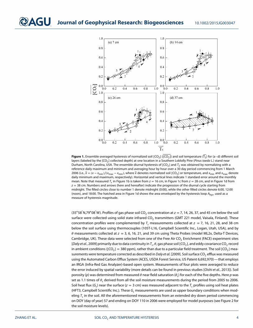
Figure 1. Ensemble-averaged hysteresis of normalized soil [CO2] ([CO2]) and soil temperature (TS) for (a–d) different soillayers (labeled by the [CO2] collected depth) at one location in a Southern Loblolly Pine (Pinus taeda L.) stand nearDurham, North Carolina, USA. The ensemble diurnal hysteresis of [CO2] and TS was obtained by normalizing with areference daily maximum and minimum and averaging hour by hour over a 30 day period commencing from 1 March2006 (i.e., x = (x − xmin)∕(xmax − xmin), where x denotes normalized soil [CO2] or temperature, and xmin and xmax denotedaily minimum and maximum, respectively). Horizontal and vertical lines indicate 1 standard error around the monthlymean. Note that measured Ts in Figure 1b is taken from z = 16 cm, in Figure 1c from z = 28 cm, and in Figure 1d fromz = 38 cm. Numbers and arrows (here and hereafter) indicate the progression of the diurnal cycle starting frommidnight. The filled circles close to number 1 denote midnight (0:00), while the other filled circles denote 6:00, 12:00(noon), and 18:00. The hatched area in Figure 1d shows the area enveloped by the hysteresis loop Ahys, used as ameasure of hysteresis magnitude.

(35∘58′N,79∘08

′W). Profiles of gas phase soil CO2 concentration at z = 7, 14, 26, 37, and 45 cm below the soil

surface were collected using solid state infrared CO2 transmitters (GMT 221 model, Vaisala, Finland). Theseconcentration profiles were complemented by Ts measurements collected at z = 7, 16, 21, 28, and 38 cmbelow the soil surface using thermocouples (105T-L16, Campbell Scientific Inc., Logan, Utah, USA), and by𝜃 measurements collected at z = 3, 6, 16, 21, and 39 cm using Theta Probes (model ML2x, Delta-T Devices,Cambridge, UK). These data were selected from one of the Free Air CO2 Enrichment (FACE) experiment sites[Daly et al., 2009] primarily due to data continuity in Ts, 𝜃, gas phase soil [CO2], and eddy covariance CO2 recordin ambient conditions ([CO2] = 380 ppm), rather than due to a particular field treatment. The soil [CO2] mea-surements were temperature corrected as described in Daly et al. [2009]. Soil surface CO2 efflux was measuredusing the Automated Carbon Efflux System (ACES, USDA Forest Service, US Patent 6,692,970)—that employsan IRGA (Infra-Red Gas Analyzer)-based open system. Measurements of four plots were averaged to reducethe error induced by spatial variability (more details can be found in previous studies [Oishi et al., 2013]). Soilporosity (p) was determined from measured 𝜃 near field saturation (𝜃s) for each of the five depths. Here p wasset as 1.1 times of 𝜃s derived from all the soil moisture measurements during the period from 2005 to 2006.Soil heat flux (Gs) near the surface (z = 3 cm) was measured adjacent to the Ts profiles using soil heat plates(HFT3, Campbell Scientific Inc.). These Gs measurements are used as upper boundary conditions when mod-eling Ts in the soil. All the aforementioned measurements from an extended dry down period commencingon DOY (day of year) 57 and ending on DOY 110 in 2006 were employed for model purposes (see Figure 2 forthe soil moisture levels).



Figure 2. Measured soil moisture series during the selected dry downat various soil depths (from DOY 57 to 110 in 2006). The eightvertical dashed lines denote the eight levels of selected soil wetnessused in the model runs as prototypical of various soil moisture states.The commonly used soil moisture shape is the fourth profile(unless otherwise stated).

2.2. The CO2 Transport ModelTo explore the onset of the hysteretic F-Ts

and [CO2]-Ts relations at different depthsand across a wide range of soil moistureconditions, a one-dimensional CO2 trans-port model is employed. The model isbased on the continuity equation for gasphase CO2 given by

𝜕fa[CO2]𝜕t

= −𝜕F(z)𝜕z

+ S(z), (1)

where fa is the air-filled porosity (fa=p−𝜃),F(z) is the CO2 flux at depth z withF(0) = Rs (soil respiration), and S(z) is alocal source of CO2 associated with rootand microbial respiration. Because dif-fusive effects govern CO2 movement inthe soil, the vertical CO2 flux can beexpressed as

F(z) = −D(𝜃, Ts)𝜕[CO2]𝜕z

, (2)

where D(.) is the soil gas phase diffusivity of CO2 estimated as [Millington and Quirk, 1961]

D(𝜃, Ts) = Da

(Ts + 273

293

)1.75 f 𝛼ap2

, (3)

where Da (= 0.157 cm2 s−1) is the free air CO2 diffusion coefficient at 20∘C (i.e., 293 K), and 𝛼 (= 10∕3) is anempirical coefficient determined for this soil type using an independent data set as described in Suwa et al.[2004]. Several formulations for the diffusivity-soil-moisture relations are also available, but they share a similarpower law behavior, apart from a rather old and seldom used equation by Penman [Blagodatsky and Smith,2012, Figure 3]. Relative differences among formulations may become important near saturation, as modelsbased on a percolation threshold predict zero diffusivity when this air-filled porosity threshold is crossed,whereas the others reach zero diffusivity only at full saturation. The analysis here considers soil moisture valuesfar from saturation, and thus the model runs are all performed in conditions where differences among modelsare not expected to be large as discussed elsewhere [Suwa et al., 2004]. Therefore, the results for the commonlyused Millington and Quirk model are used here with 𝛼 set to 10∕3 as determined from prior experiments atthe site.

In all model runs, the top 50 cm of the soil was vertically divided into five layers of dz = 10 cm thickness, witheach layer center treated as a computational node (i.e., 5, 15, 25, 35, and 45 cm). As upper boundary conditionof the [CO2] model, the [CO2] at 0 cm was set to ambient atmospheric conditions (= 380 ppm). The diurnalvariation of this upper boundary condition (< 20 ppm) is not likely to affect the outcome appreciably giventhat the [CO2] in the first layer exceeds 2000 ppm. The lower boundary condition was treated as a zero flux(i.e., F(z) = 0 at z = 45 cm).

2.3. The Determination of the Source TermThe soil CO2 production term depends on several biotic and abiotic factors. To explore these biotic and abi-otic controls on the [CO2]-Ts and Rs-Ts hystereses sequentially, a set of calculations is proposed with varyingdegrees of complexities in representing S(z, t). The simplest representation is given as

S(z, t) = Sref(z)eb(z)Ts(z,t), (4)

where Sref is the base CO2 production reflecting root density and SOC vertical distribution, and b is a localtemperature sensitivity parameter related to the Q10 coefficient via Q10 = e10b.



The simultaneous effects of Ts and 𝜃 are considered next using [Davidson et al., 1998]

S(z, t) = STs−𝜃(z)ebTs (z)Ts(z,t)+b𝜃(z)

𝜃(z,t)p(z) , (5)

where STs−𝜃 , bTs, and b𝜃 are fitting parameters.

The two different S calculation methods in equations (4) and (5) account for two possible scenarios of soil CO2

production. In general, soil CO2 production is temperature dependent provided appropriate soil moisturelevels are maintained (equation (4)), while in many field conditions, soil temperature and moisture are bothcontrolling factors of soil CO2 production (equation (5)) [Davidson et al., 1998].

In addition to Ts and 𝜃, photosynthesis is also suggested to be a factor controlling soil CO2 production byproviding photosynthate for root and rhizospheric respiration. To accommodate this scenario, it is assumedthat the temperature sensitivity of CO2 production remains unchanged (i.e., parameter b(z) in equation (4)),but Sref in equation (4) was further modified to account for the effect of photosynthesis on microbial and rootrespiration. Temporal patterns (not actual magnitudes) of canopy photosynthesis were surrogated to grossprimary productivity (GPP) inferred from eddy covariance measurements collected at the site (see Figure S1in the supporting information) and a time lag, 𝜏 , between soil CO2 production and photosynthesis was thenassumed. Hence, when including photosynthesis, Sref was modified to combine the base line CO2 productionand a rhizosphere component that depends on GPP. The Sref was thus corrected by the rate modifier,

𝜒 = 12

[1 + GPP(t − 𝜏)

GPPmax

], (6)

where GPPmax denotes the maximum of a diurnal GPP series, and the effect of photosynthesis is delayed by𝜏 . The S resulting from photosynthesis is determined by multiplying equations (4) and (6) while keeping b(z)unchanged. Again, the main goal here is to construct possible conditions on S so as to explore the Rs-Ts and[CO2]-Ts hystereses, not the absolute values of S of the long-term data set.

To derive plausible parameters for different methods, the source term S was estimated from measurementsof soil [CO2], Ts, and 𝜃 using equation (1). A quadratic function was used to fit the soil [CO2] profiles only fornumerical differentiation purposes [Daly et al., 2009].

The values of Sref and b (equation (4)), STs−𝜃 , bTs, and b𝜃 (equation (5)) at different depths were optimized using

calculated S(z), measured 𝜃(z) and Ts(z). Negative S inferred within the three days after a rain event werediscarded.

2.4. Heat Flow ModelThe CO2 transport model in equation (1) requires the variations in Ts(z, t), which were modeled by combiningFourier’s heat conduction law with a heat budget equation given as

Cp(𝜃)𝜕Ts(z, t)

𝜕t= 𝜕

𝜕z

[𝜆(𝜃)

𝜕Ts(z, t)𝜕z

], (7)

where Cp is the soil specific heat capacity and 𝜆 is the soil thermal conductivity [Johansen, 1975]. The soilvolumetric specific heat capacity was expressed as Cp(𝜃) = 𝜃C𝜃 + (1−p)Cs, neglecting the contribution of air;C𝜃 = 4.18 J cm−3 ∘C−1 and Cs are the water and soil heat capacity with Cs determined as

Cs(z) = 0.85𝜌b(z), (8)

where 𝜌b (g cm−3) is the soil bulk density measured by Oh and Richter [2005]. The top 100 cm of the soil wasdivided into 50 layers of 2 cm thickness with the center of each layer treated as a computational node fornumerical calculations of heat flow. Measured subsurface soil heat flux (at z = 3 cm) was used as a boundarycondition at the surface, and zero heat flux was imposed at the bottom of the 100 cm domain.

2.5. Numerical RunsA hierarchy of numerical model runs were conducted to determine the onset and magnitude of the hysteretic[CO2]-Ts and F-Ts relations at different z in the absence of space-time variations in soil moisture.

As gas transport and heat flow are both potential factors responsible for the hysteresis, the first set ofruns was designed to disentangle them. To achieve this goal, this set of runs is purely hypothetical based



on prescribed soil conditions by assuming that soil texture is vertically uniform with soil porosity set to

p(z) = 0.5 m3 m−3. Soil temperature was also set vertically uniform (equivalent to assuming 𝜆 → ∞), and all

depths had identical diurnal variations in Ts to investigate the role of gas transport alone in controlling the

aforementioned hysteresis. Two scenarios for S are considered: (1) the source term S was set vertically homo-

geneous with S(z) = 2 μmol m−3 s−1 to investigate the onset of hysteresis evolution; (2) S(z) was determined

using equation (4) by considering controls of the temporally fluctuating soil temperature but with vertically

homogeneous parameters (Sref(z) = 1μmol m−3 s−1, b(z) = 0.1∘C−1). These values, while arbitrarily set, remain

within reasonable ranges when depth integrated to yield Rs. Heat flow was then included to generate soil

temperature profiles under finite 𝜆 so as to investigate the effects of heat flow on [CO2]-Ts and F-Ts hystereses.

The parameters of S were also set vertically homogeneous with Sref(z) = 1 μmol m−3 s−1 and b(z) = 0.1∘C−1.

The runs were all conducted under different soil moisture levels but assuming their profiles to be momentarily

uniform (i.e., 𝜃(z) = 0.1 to 0.45 m3 m−3 with increment of 0.05 m3 m−3).

In the second set of runs, measured 𝜃(z) for eight contrasting levels (see Figure 2) sampled during the selected

dry down period were used as prototypical soil moisture profiles. The two different S calculation methods (i.e.,

equations (4) and (5)) were then applied, and the parameters were determined as described in section 2.3

(see Figure S2 and Table S1 in the supporting information for details). These runs allow for investigating the

hysteretic [CO2]-Ts and F-Ts relations in realistic field conditions where soil wetness impacts simultaneously

heat flow and gas movement, but still without plant-derived C.

The third set of runs incorporates the effects of lagged photosynthesis on soil CO2 production (combining

equations (4) and (6)) while maintaining the same 𝜃(z) profile shape as that in the second set of runs. Because

the focus here is on diurnal hysteresis, only subdaily time lags were considered (only 𝜏 = 0, 4, 6, and 7 h as

typical cases are shown in this study).

To allow the CO2 transport model to reach “equilibrium,” a continuous simulation period of 600 days with

1 min integration time step (= dt) was employed for all runs using concentration measurements at the begin-

ning of the selected period (i.e., DOY = 57) as initial conditions. Note that the soil moisture profiles were

unchanged in the first set of runs (i.e., 𝜃(z) = 0.1, 0.15, ... , 0.45 m3 m−3). In the second and third sets of runs,

the eight levels of soil moisture profiles in Figure 2 were used across the entire simulation period regardless

of the natural soil moisture fluctuation, as the purpose is to achieve steady state soil [CO2] profiles and F(z)in equilibrium with a local soil moisture regime and analyze the hysteresis at this equilibrium soil moisture

state. The 600 day period was selected to ensure sufficient integration time to attain equilibration between

CO2 concentration and fluxes and the imposed soil moisture regime for time-varying soil temperature and

GPP. All simulations exhibited a near-stationary state in [CO2] at all layers by the end of the 600 days simula-

tion period. In many cases, [CO2] exhibited oscillatory but stationary behavior by the end of the simulation

period (see Figure S3).

Previous studies investigated the apparent hysteretic relation between Rs (i.e., F(0)) and Ts measured at some

arbitrary depth (e.g., z = 2, 5, 10 cm, etc.). The consequence of this variable choice of a Ts depth on the F(0)-Ts

hysteresis has been studied and is not elaborated on here. Different from these earlier studies, the focus here

is on F(z) (also [CO2]) and Ts(z) hysteresis when colocated at the same depth z. As F(z) is calculated with a

model based on CO2 gradient method, F(z) represents an average flux between two [CO2] depths, and hence,

the corresponding averaged temperature between the two depths was used as the Ts corresponding to F(z).

To obtain temperature variations for the numerical runs of the CO2 transport model, periodic diurnal soil heat

flux series (see Figure S4 in the supporting information) was used to drive Ts for the prescribed soil moisture

levels (that are assumed or measured). However, surface temperature variation was applied in the scenario of

infinite thermal conductivity (first set). To standardize the soil temperature calculations across scenarios, a uni-

form soil temperature (≈ 10.5∘C) was set as initial condition for all heat flow model runs, and a near-stationary

state was reached with temperature changing periodically at the end of simulation. The simulation length

was set as 10 days, because temperature simulations reach a steady state in a relatively shorter time when

compared to gas phase CO2. Because the thermal conductivity and the specific heat capacity depend on 𝜃,

different soil temperature profiles emerged due to different soil moisture levels by the end of model runs.



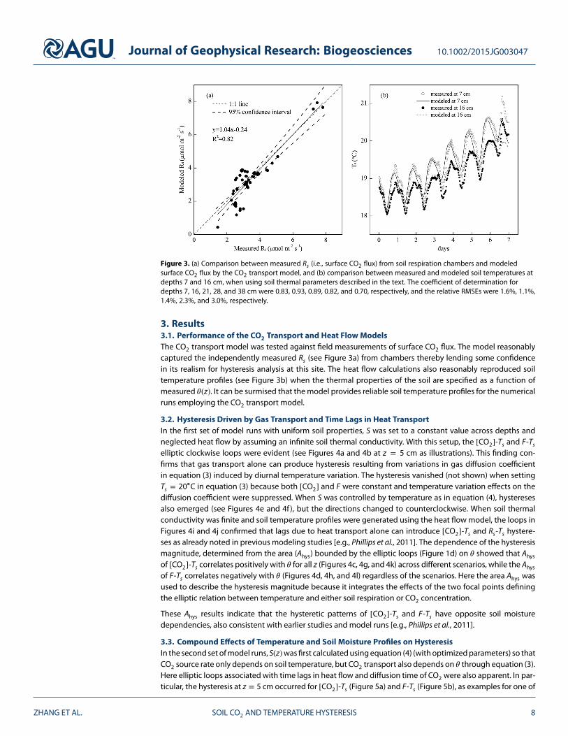
Figure 3. (a) Comparison between measured Rs (i.e., surface CO2 flux) from soil respiration chambers and modeledsurface CO2 flux by the CO2 transport model, and (b) comparison between measured and modeled soil temperatures atdepths 7 and 16 cm, when using soil thermal parameters described in the text. The coefficient of determination fordepths 7, 16, 21, 28, and 38 cm were 0.83, 0.93, 0.89, 0.82, and 0.70, respectively, and the relative RMSEs were 1.6%, 1.1%,1.4%, 2.3%, and 3.0%, respectively.

3. Results3.1. Performance of the CO2 Transport and Heat Flow ModelsThe CO2 transport model was tested against field measurements of surface CO2 flux. The model reasonablycaptured the independently measured Rs (see Figure 3a) from chambers thereby lending some confidencein its realism for hysteresis analysis at this site. The heat flow calculations also reasonably reproduced soiltemperature profiles (see Figure 3b) when the thermal properties of the soil are specified as a function ofmeasured 𝜃(z). It can be surmised that the model provides reliable soil temperature profiles for the numericalruns employing the CO2 transport model.

3.2. Hysteresis Driven by Gas Transport and Time Lags in Heat TransportIn the first set of model runs with uniform soil properties, S was set to a constant value across depths andneglected heat flow by assuming an infinite soil thermal conductivity. With this setup, the [CO2]-Ts and F-Ts

elliptic clockwise loops were evident (see Figures 4a and 4b at z = 5 cm as illustrations). This finding con-firms that gas transport alone can produce hysteresis resulting from variations in gas diffusion coefficientin equation (3) induced by diurnal temperature variation. The hysteresis vanished (not shown) when settingTs = 20∘C in equation (3) because both [CO2] and F were constant and temperature variation effects on thediffusion coefficient were suppressed. When S was controlled by temperature as in equation (4), hysteresesalso emerged (see Figures 4e and 4f), but the directions changed to counterclockwise. When soil thermalconductivity was finite and soil temperature profiles were generated using the heat flow model, the loops inFigures 4i and 4j confirmed that lags due to heat transport alone can introduce [CO2]-Ts and Rs-Ts hystere-ses as already noted in previous modeling studies [e.g., Phillips et al., 2011]. The dependence of the hysteresismagnitude, determined from the area (Ahys) bounded by the elliptic loops (Figure 1d) on 𝜃 showed that Ahys

of [CO2]-Ts correlates positively with 𝜃 for all z (Figures 4c, 4g, and 4k) across different scenarios, while the Ahys

of F-Ts correlates negatively with 𝜃 (Figures 4d, 4h, and 4l) regardless of the scenarios. Here the area Ahys wasused to describe the hysteresis magnitude because it integrates the effects of the two focal points definingthe elliptic relation between temperature and either soil respiration or CO2 concentration.

These Ahys results indicate that the hysteretic patterns of [CO2]-Ts and F-Ts have opposite soil moisturedependencies, also consistent with earlier studies and model runs [e.g., Phillips et al., 2011].

3.3. Compound Effects of Temperature and Soil Moisture Profiles on HysteresisIn the second set of model runs, S(z)was first calculated using equation (4) (with optimized parameters) so thatCO2 source rate only depends on soil temperature, but CO2 transport also depends on 𝜃 through equation (3).Here elliptic loops associated with time lags in heat flow and diffusion time of CO2 were also apparent. In par-ticular, the hysteresis at z = 5 cm occurred for [CO2]-Ts (Figure 5a) and F-Ts (Figure 5b), as examples for one of



Figure 4. Results of the first set of runs for hysteresis at depth z = 5 cm when 𝜃(z) = 0.25 m3 m−3 (shown as example). Soil temperature that is vertically uniform(by assuming an infinite thermal conductivity), with (a) [CO2]-Ts and (b) Rs-Ts showing relations with constant source term S. (e and f) Runs undertemperature-dependent S scenario (i.e., S determined by equation (4)). (i and j) Runs when the soil temperature profile is driven by field measured heat fluxsubjected to typical field thermal properties and S is temperature-dependent (i.e., S determined by equation (4)). The numbers and arrows indicate theprogression during the day, number 1 corresponds to midnight. (c and d), (g and h), and (k and l) Dependencies of the hysteresis area (Ahys) on soil moisture for[CO2]-Ts and F-Ts for the three different scenarios, respectively.

Figure 5. Results of the second set of runs under realistic moisture and temperature field conditions and optimized parameters of the source term S. Hysteresisat z = 5 cm are shown as examples for the fourth soil moisture level. (a) [CO2]-Ts and (b) Rs-Ts relations when S only depends on Ts (equation (4)); (e and f) thesame relations as in Figures 5a and 5b when S also depends on 𝜃 (equation (5)). The numbers and arrows indicate the progression during the day, number 1corresponds to midnight. (c and d) The corresponding dependencies of Ahys for [CO2]-Ts and F-Ts on soil moisture at different depths when S is determined byequation (4); (g and h) similar dependencies as in Figures 5c and 5d when S is determined by equation (5).



Figure 6. Hysteresis at different depths and soil moisture levels when the source term S only depends on Ts (equation (4)) in the second set of runs. (a–d) and(i–l) [CO2]-Ts and F-Ts hysteresis for the wettest soil conditions (i.e., first soil moisture level in Figure 2); (e–h) and (m–p) those for the driest soil conditions (i.e.,eighth soil moisture level in Figure 2). Note that all modeled hysteresis loops exhibit counterclockwise directions.

the 𝜃(z)profiles (fourth profile shown in Figure 2); other depths had similar loop patterns as shown in Figure 6.The [CO2]-Ts hysteresis exhibited counterclockwise loop patterns at all depths as time progresses (starting atmidnight), and [CO2] correlated positively with Ts. Regarding the F(z)-Ts(z) relation, the hysteresis at all z alsoexhibited counterclockwise loop patterns. However, the correlation patterns appeared to be more complex.The positive F-Ts correlation at z = 5 cm gradually degraded and switched to negative with increasing z (e.g.,z =25 and 35 cm) (Figures 6k, 6l, 6o, and 6p). At the intermediate z =15 cm, the dependence of F(z) on Ts(z)appeared weak. These results demonstrate that F(z)does not necessarily depend on temperature in a positivemanner, especially for intermediate depths where the source term S is low.

Regarding the soil moisture dependence, the hysteretic [CO2]-Ts and F-Ts relations at z = 5 cm were similar atdifferent soil moisture levels (Figure 6). Surprisingly, the Ahys of [CO2]-Ts did not correlate with 𝜃 in a monotonicmanner for z = 15, 25, and 35 cm, where one soil moisture level corresponded to a minimum Ahys (Figure 5c),whereas Ahys at z = 5 cm correlated positively with 𝜃. Consistent with the first set of runs, Ahys of the F-Ts

hysteresis correlated negatively with 𝜃 in a near-monotonic manner for all z (Figure 5d).

When both Ts and 𝜃 were simultaneously accounted for in the source term S calculation using equation (5),the hysteresis loops exhibited similar patterns and orientations (Figures 5e and 5f) as with S determined byequation (4). All the dependence of Ahys of [CO2]-Ts on 𝜃 at z = 15, 25, and 35 cm exhibited a minimum Ahys at



Figure 7. Hysteresis of soil [CO2] (a–d) and Rs (e–h) with Ts at z = 5 cm for the fourth soil moisture level using different subdaily time lags 𝜏 betweenphotosynthesis and soil CO2 production. The numbers and arrows indicate the progression during the day, number 1 corresponds to midnight.

some moisture level (Figure 5g), while Ahys for the F-Ts of all depths correlated negatively with 𝜃 in a monotonicmanner (Figure 5h), consistent with earlier results when S was determined by soil temperature alone.

In summary, the two different S calculation methods result in Ahys for F-Ts correlating negatively with increased𝜃, while the dependence of Ahys for [CO2]-Ts on 𝜃 is more complicated. There appears to be a regime whereAhys achieves a minimum for intermediate 𝜃.

3.4. Compound Effects of Soil Temperature, Moisture, and Photosynthesis on HysteresisFor the third set of runs, lagged photosynthesis was included in S by combining equations (4) and (6). Here newhysteresis loop patterns emerged for both [CO2]-Ts and Rs-Ts. Altering the time lag 𝜏 between CO2 productionand photosynthesis introduced the most dynamically interesting features in the hysteresis patterns for both[CO2]-Ts and Rs-Ts relations (Figure 7). Qualitatively, for 𝜏 = 7 h, the outcome of these model runs appearednot too different from the second set of runs in terms of loop shape and direction (see Figures 7d and 7h),respectively). Upon reducing 𝜏 , the previously reported loop direction was reversed from counterclockwise toclockwise, and an asymmetric 8-shaped pattern emerged during the transition at an intermediate 𝜏 for both[CO2]-Ts and Rs-Ts hysteresis loops (Figures 7c and 7f), where two or more “lobs” appeared in the [CO2]-Ts andRs-Ts relations.

4. Discussion and Conclusions

While several studies highlighted the presence of hysteretic loops in the soil respiration-temperature and soilCO2 concentration-temperature relations (Table 1), a unified framework that links all the main drivers for theseloops to environmental (soil moisture) and biogeochemical conditions (CO2 source versus temperature andmoisture relations; plant contributions) remains elusive. By sequentially adding contributions to CO2 produc-tion rates and transport, we identified individual and compound drivers of the hysteretic loops. Hysteresisoccurs in the absence of vertical profiles of temperature and moisture and for constant CO2 production ratebecause daily temperature fluctuations cause a daily cycle in CO2 transport rate (through thermal effects ongas diffusivity; Figures 4a and 4b). This loop is small and has clockwise direction. When temperature effectson CO2 production are added, the loop alters direction and gains in magnitude (Figures 4e–4h), but is againreduced when considering delays in temperature changes through the soil profile (Figures 4i–4l). Therefore,temperature may both enhance (through effects on S) and inhibit (when heat conduction is finite) the hys-teretic loops. As discussed next, soil moisture effects and plant contributions through photosynthesis furthercomplicate the picture.

On a diurnal basis, soil moisture fluctuations are comparatively small within the root zone and have beendiscarded as a factor responsible for the Rs-Ts hysteresis by some studies [Gaumont-Guay et al., 2006;



Figure 8. Comparisons of hysteresis loops of soil [CO2] and Rs with Ts at z = 5 cm, across the different numerical runs, (a and e) [CO2]-Ts and Rs-Ts relations whenS is set constant, thermal conductivity 𝜆 → ∞, and 𝜃 = 0.30 m3 m−3 in homogeneous soil; (b and f) S varying with temperature, thermal conductivity 𝜆 → ∞,and 𝜃 = 0.30 m3 m−3 in homogeneous soil; (c and g) S varying with temperature alone under realistic field conditions with the fourth measured soil moisturelevel; (d and h) S varying with temperature and GPP under realistic field conditions with the fourth measured soil moisture level. Arrows indicate the progressionduring the day.

Pingintha et al., 2010]. However, it is evident from the model runs here that small changes in soil moisturecan impact the Rs−Ts hysteresis magnitude at a given z (Figures 4d, 4h, and 4l). Regarding the near-surface[CO2]-Ts hysteresis, Riveros-Iregui et al. [2007] suggested that higher soil moisture results in hysteresis withlarger magnitude (Quantified by the maximum width of the elliptic shape of the hysteresis loop insteadof its area as used here). This argument agrees with the model calculations here for near-surface [CO2]when S is constant or only temperature dependent (Figures 4c, 4g, 4k, and 5c). In this scenario, S is con-trolled by soil temperature alone, while CO2 diffusion is mainly controlled by soil moisture. Reductions inCO2 diffusion coefficient with increased 𝜃 enhance CO2 buildup, thereby causing larger [CO2]-Ts hysteresis.However, soil moisture has a more complicated control on the hysteresis magnitude at intermediate depths(e.g., z = 15 and 25 cm in Figure 5c and also Figure 5g). These patterns may also depend on the inverse relationbetween S and 𝜃 in this ecosystem (i.e., b𝜃 < 0 in equation (5)), which indicates oxygen as limitation to micro-bial metabolism, rather than moisture limitation as often observed during extended dry downs [Manzoniet al., 2012].

The effects of photosynthesis on soil CO2 were reported with delays ranging from hours to weeks depend-ing on plant size [Kuzyakov and Cheng, 2001; Stoy et al., 2007; Baldocchi et al., 2006; Detto et al., 2012; Zhanget al., 2013]. Therefore, we may expect that even at subdaily scales considered here, photosynthesis mightcontribute to CO2 concentration and flux dynamics. Though photosynthesis may not be necessary for pro-ducing hysteresis, the model results here suggest that the lag between photosynthesis and S can introducecomplex [CO2]-Ts and F-Ts hysteretic patterns, in which the directions of the loops can be reversed undervarious subdaily time lags. For time lags of the order of 7 h, both [CO2]-Ts and F-Ts hystereses exhibited coun-terclockwise looping directions with increasing time similar to the field conditions (Figure 1). For time lagof 0 h, the hysteresis directions were clockwise for both [CO2]-Ts and F-Ts hystereses. However, this afore-mentioned case cannot occur as finite time lags between rhizospheric CO2 production and photosynthesismust always exist due to photosynthate travel times. At the transition between counterclockwise and clock-wise directions at intermediate time lag levels, an asymmetric 8-shaped hysteretic pattern appeared in both[CO2]-Ts and F-Ts (Figures 7c and 7f). Field evidence for this 8-shaped [CO2]-Ts pattern (Figure 1) was notedin previous experiments [Riveros-Iregui et al., 2007]. Likewise, a similar 8-shaped hysteretic Rs-Ts pattern was



also reported in other field studies, [e.g., Parkin and Kaspar, 2003; Bahn et al., 2008; Barron-Gafford et al., 2011;Jia et al., 2013].

Interestingly, both clockwise and counterclockwise directions in the Rs-Ts hysteresis pattern were reportedin experiments (Table 1). Most reported Rs rates were related to a subsurface Ts at depth z. Hence, some ofthe reported inconsistencies in loop directions result from differences in soil depths selected when analyzingTs. Removing such inconsistency (in model runs for Rs and Ts) showed that different S dependence scenarioscan result in hysteresis with different directionality. For example, when S is only temperature dependent, the[CO2]-Ts and Rs-Ts hystereses are mostly counterclockwise (Figure 6). The inclusion of lagged photosynthe-sis as a driver of soil CO2 production can alter the hysteresis direction. This finding suggests that the time lagbetween soil CO2 production and photosynthesis may be indirectly estimated by analyzing simultaneouslythe hysteresis loop patterns and directions at subdaily time scales. In previous studies (including ours), soilrespiration was not separated into its autotrophic and heterotrophic components. Both autotrophic and het-erotrophic respiration components exhibit hysteretic responses to Ts [Savage et al., 2013], but these twocomponents may exhibit opposite hysteresis directions. Whether measured hysteresis looping directions mayaid in discriminating between autotrophic and heterotrophic dominance on Rs is an interesting question forthe future.

Generally, the magnitudes of both [CO2]-Ts and Rs-Ts hysteretic loops are not large because of the small diurnaltemperature variation in the forested ecosystem considered here. Using additional model runs, it is shownthat amplifying these diurnal temperature variations has a positive effect (not shown) on the magnitude ofthe hysteresis, consistent with other studies [e.g., Riveros-Iregui et al., 2007].

The numerical experiment setup here provides a “catalog” summary on how different factors contribute to theevolutions of [CO2]-Ts and Rs-Ts hystereses, as illustrated in Figure 8 for the 5 cm depth. In homogeneous soil,when setting S constant and assuming thermal conductivity 𝜆→∞, the [CO2]-Ts hysteresis exhibits clockwisedirection with [CO2] correlating negatively with Ts (Figure 8a), and Rs-Ts also exhibits clockwise direction withRs correlating with Ts in a positive manner (Figure 8e). These patterns are driven by the diffusion coefficientvariations due to diurnal temperature fluctuations. When S varies with Ts following the exponential depen-dence in equation (4), both [CO2]-Ts and Rs-Ts hystereses exhibit counterclockwise directions, and both [CO2]and Rs correlate positively with Ts (Figures 8b and 8f); these patterns are similar under realistic field conditions(Figures 8c and 8g). Incorporating the effects of heat flow, temperature, and GPP dependencies of S, differenttime lag levels of 𝜏 = 0 h and 𝜏 = 7 h result in hysteresis with different directions and patterns (Figures 8dand 8h). To what extent this summary holds across other sites and ecosystems, and how to improve soil res-piration simulation by incorporating the hysteresis mechanisms require further field exploration and modeldevelopment.

ReferencesBahn, M., et al. (2008), Soil respiration in European grasslands in relation to climate and assimilate supply, Ecosystems, 11(8), 1352–1367.Baldocchi, D., J. W. Tang, and L. K. Xu (2006), How switches and lags in biophysical regulators affect spatial-temporal variation of soil

respiration in an oak-grass savanna, J. Geophys. Res., 111, G02008, doi:10.1029/2005JG000063.Barron-Gafford, G. A., R. L. Scott, G. D. Jenerette, and T. E. Huxman (2011), The relative controls of temperature, soil moisture, and plant

functional group on soil CO2 efflux at diel, seasonal, and annual scales, J. Geophys. Res., 116, G01023, doi:10.1029/2010JG001442.Blagodatsky, S., and P. Smith (2012), Soil physics meets soil biology: Towards better mechanistic prediction of greenhouse gas emissions

from soil, Soil Biol. Biochem., 47, 78–92.Buysse, P., S. Goffin, M. Carnol, S. Malchair, A. Debacq, B. Longdoz, and M. Aubinet (2013), Short-term temperature impact on soil

heterotrophic respiration in limed agricultural soil samples, Biogeochemistry, 112( 1-3), 441–455.Carbone, M. S., G. C. Winston, and S. E. Trumbore (2008), Soil respiration in perennial grass and shrub ecosystems: Linking environmental

controls with plant and microbial sources on seasonal and diel timescales, J. Geophys. Res., 113, G02022, doi:10.1029/2007JG000611.Daly, E., A. C. Oishi, A. Porporato, and G. G. Katul (2008), A stochastic model for daily subsurface CO2 concentration and related soil

respiration, Adv. Water Res., 31(7), 987–994.Daly, E., S. Palmroth, P. Stoy, M. Siqueira, A. C. Oishi, J. Y. Juang, R. Oren, A. Porporato, and G. G. Katul (2009), The effects of elevated

atmospheric CO2 and nitrogen amendments on subsurface CO2 production and concentration dynamics in a maturing pine forest,Biogeochemistry, 94(3), 271–287.

Davidson, E. A., E. Belk, and R. D. Boone (1998), Soil water content and temperature as independent or confounded factors controlling soilrespiration in a temperate mixed hardwood forest, Global Change Biol., 4(2), 217–227.

Davidson, E. A., L. V. Verchot, J. H. Cattanio, I. L. Ackerman, and J. E. M. Carvalho (2000), Effects of soil water content on soil respiration inforests and cattle pastures of eastern Amazonia, Biogeochemistry, 48(1), 53–69.

Detto, M., A. Molini, G. Katul, P. Stoy, S. Palmroth, and D. Baldocchi (2012), Causality and persistence in ecological systems: A nonparametricspectral granger causality approach, Am. Nat., 179(4), 524–535.

Fu, X. L., M. A. Shao, X. R. Wei, and H. M. Wang (2013), Soil respiration as affected by vegetation types in a semiarid region of China, Soil Sci.Plant Nutr., 59(5), 715–726.

AcknowledgmentsThe authors thank A. Porporato andE. Ward for valuable discussions,C. Oishi for providing soil surfaceCO2 efflux data for model validation,the Editors, C. Phillips and reviewerswho provided constructive criticisms.This work was supported in partby the United States Departmentof Energy (DOE) through the Officeof Biological and EnvironmentalResearch’s (BER) Terrestrial EcosystemScience(DE-SC0006967) and TerrestrialProcesses(DE-FG02-95ER6208)programs, the U.S. Departmentof Agriculture(2011-67003-30222),the National Science Foundation(NSF-AGS-1102227 and (DEB-1145875/1145649), and the National NaturalScience Fund of China forDistinguished Young Scholars (project51025931). Q. Zhang is supported byChina Postdoctoral Science Foundation(project 2015M570662) andfoundation for young scholarsat Wuhan University (project206-410500128); Data sets for thispaper are available upon request bycontacting the corresponding author(Q. Zhang, [email protected]).


http://dx.doi.org/10.1029/2005jg000063

http://dx.doi.org/10.1029/2010JG001442

http://dx.doi.org/10.1029/2007JG000611


Gaumont-Guay, D., T. A. Black, T. J. Griffis, A. G. Barr, R. S. Jassal, and Z. Nesic (2006), Interpreting the dependence of soil respiration on soiltemperature and water content in a boreal aspen stand, Agric. For. Meteorol., 140(1-4), 220–235.

Janssens, I. A., et al. (2010), Reduction of forest soil respiration in response to nitrogen deposition, Nat. Geosci., 3(5), 315–322.Jia, X., T. S. Zha, B. Wu, Y. Q. Zhang, W. J. Chen, X. P. Wang, H. Q. Yu, and G. M. He (2013), Temperature response of soil respiration in a Chinese

pine plantation: Hysteresis and seasonal vs. diel Q10, Plos One, 8(2), E57858, doi:10.1371/journal.pone.005785.Johansen, O. (1975), Thermal conductivity of soils (in Norwegian), PhD thesis, Univ. of Trondheim, Trondheim, Norway. (English

Translation, No. 637, Cold Reg. Res. and Eng. Lab., Hanover, N. H., 1977).Jones, D. L., and D. V. Murphy (2007), Microbial response time to sugar and amino acid additions to soil, Soil Biol. Biochem., 39(8), 2178–2182.Kuzyakov, Y., and W. Cheng (2001), Photosynthesis controls of rhizosphere respiration and organic matter decomposition, Soil Biol.

Biochem., 33(14), 1915–1925.Li, Z. G., X. J. Wang, R. H. Zhang, J. Zhang, and C. Y. Tian (2011), Contrasting diurnal variations in soil organic carbon decomposition and root

respiration due to a hysteresis effect with soil temperature in a Gossypium s. (cotton) plantation, Plant Soil, 343(1-2), 347–355.Lloyd, J., and J. A. Taylor (1994), On the temperature-dependence of soil respiration, Funct. Ecol., 8(3), 315–323.Manzoni, S., J. P. Schimel, and A. Porporato (2012), Responses of soil microbial communities to water stress: Results from a meta-analysis,

Ecology, 93(4), 930–938.Millington, R., and J. P. Quirk (1961), Permeability of porous solids, Trans. Faraday Soc., 57(8), 1200–1207.Oh, N.-H., and D. D. Richter (2005), Elemental translocation and loss from three highly weathered soil-bedrock profiles in the southeastern

United States, Geoderma, 126(1-2), 5–25.Oikawa, P. Y., D. A. Grantz, A. Chatterjee, J. E. Eberwein, L. A. Allsman, and G. D. Jenerette (2014), Unifying soil respiration pulses,

inhibition, and temperature hysteresis through dynamics of labile soil carbon and O2, J. Geophys. Res. Biogeosci., 119, 521–536,doi:10.1002/2013JG002434.

Oishi, A. C., S. Palmroth, J. R. Butnor, K. H. Johnsen, and R. Oren (2013), Spatial and temporal variability of soil CO2 efflux in three proximatetemperate forest ecosystems, Agric. For. Meteorol., 171-172, 256–269.

Palmroth, S., R. Oren, H. R. McCarthy, K. H. Johnsen, A. C. Finzi, J. R. Butnor, M. G. Ryan, and W. H. Schlesinger (2006), Aboveground sinkstrength in forests controls the allocation of carbon below ground and its [CO2]-induced enhancement, Proc. Natl. Acad. Sci. USA,103(51), 19,362–19,367.

Parkin, T. B., and T. C. Kaspar (2003), Temperature controls on diurnal carbon dioxide flux: Implications for estimating soil carbon loss, SoilSci. Soc. Am. J., 67(6), 1763–1772.

Phillips, C. L., N. Nickerson, D. Risk, and B. J. Bond (2011), Interpreting diel hysteresis between soil respiration and temperature, GlobalChange Biol., 17(1), 515–527.

Phillips, S. C., R. K. Varner, S. Frolking, J. W. Munger, J. L. Bubier, S. C. Wofsy, and P. M. Crill (2010), Interannual, seasonal, and diel variationin soil respiration relative to ecosystem respiration at a wetland to upland slope at Harvard Forest, J. Geophys. Res., 115, G02019,doi:10.1029/2008JG000858.

Pingintha, N., M. Y. Leclerc, J. P. Beasley, G. S. Zhang, and C. Senthong (2010), Assessment of the soil CO2 gradient method for soil CO2 effluxmeasurements: Comparison of six models in the calculation of the relative gas diffusion coefficient, Tellus B, 62( 1), 47–58.

Raich, J. W., and W. H. Schlesinger (1992), The global carbon-dioxide flux in soil respiration and its relationship to vegetation and climate,Tellus B, 44(2), 81–99.

Risk, D., L. Kellman, and H. BeltRami (2002), Carbon dioxide in soil profiles: Production and temperature dependence, Geophys. Res. Lett.,29(6), 1087, doi:10.1029/2001GL014002.

Riveros-Iregui, D. A., R. E. Emanuel, D. J. Muth, B. L. McGlynn, H. E. Epstein, D. L. Welsch, V. J. Pacific, and J. M. Wraith (2007), Diurnal hysteresisbetween soil CO2 and soil temperature is controlled by soil water content, Geophys. Res. Lett., 34, L17404, doi:10.1029/2007GL030938.

Ruehr, N. K., A. Knohl, and N. Buchmann (2010), Environmental variables controlling soil respiration on diurnal, seasonal and annualtime-scales in a mixed mountain forest in Switzerland, Biogeochemistry, 98(1-3), 153–170.

Savage, K., E. A. Davidson, and J. Tang (2013), Diel patterns of autotrophic and heterotrophic respiration among phenological stages, GlobalChange Biol., 19(4), 1151–1159.

Stoy, P. C., S. Palmroth, A. C. Oishi, M. B. S. Siqueira, J. Y. Juang, K. A. Novick, E. J. Ward, G. G. Katul, and R. Oren (2007), Are ecosystem carboninputs and outputs coupled at short time scales? A case study from adjacent pine and hardwood forests using impulse-responseanalysis, Plant Cell Environ., 30(6), 700–710.

Subke, J. A., and M. Bahn (2010), On the ’temperature sensitivity’ of soil respiration: Can we use the immeasurable to predict the unknown?,Soil Biol. Biochem., 42(9), 1653–1656.

Suwa, M., G. G. Katul, R. Oren, J. Andrews, J. Pippen, A. Mace, and W. H. Schlesinger (2004), Impact of elevated atmospheric CO2 on forestfloor respiration in a temperate pine forest, Global Biogeochem. Cycles, 18, GB2013, doi:10.1029/2003GB002182.

Tang, J. W., D. D. Baldocchi, and L. Xu (2005), Tree photosynthesis modulates soil respiration on a diurnal time scale, Global Change Biol.,11(8), 1298–1304.

Thomas, A. D., and S. R. Hoon (2010), Carbon dioxide fluxes from biologically-crusted Kalahari Sands after simulated wetting, J. Arid. Environ.,74(1), 131–139.

Updegraff, K., S. D. Bridgham, J. Pastor, and P. Weishampel (1998), Hysteresis in the temperature response of carbon dioxide and methaneproduction in peat soils, Biogeochemistry, 43(3), 253–272.

Vargas, R., and M. F. Allen (2008a), Diel patterns of soil respiration in a tropical forest after Hurricane Wilma, J. Geophys. Res., 113, G03021,doi:10.1029/2007JG000620.

Vargas, R., and M. F. Allen (2008b), Environmental controls and the influence of vegetation type, fine roots and rhizomorphs on diel andseasonal variation in soil respiration, New Phytol., 179(2), 460–471.

Vargas, R., and M. F. Allen (2008c), Dynamics of fine root, fungal rhizomorphs, and soil respiration in a mixed temperate forest: Integratingsensors and observations, Vadose Zone J., 7(3), 1055–1064.

Wan, S. Q., and Y. Q. Luo (2003), Substrate regulation of soil respiration in a tallgrass prairie: Results of a clipping and shading experiment,Global Biogeochem. Cycles, 17(2), 1054, doi:10.1029/2002GB001971.

Wang, B., T. S. Zha, X. Jia, B. Wu, Y. Q. Zhang, and S. G. Qin (2014), Soil moisture modifies the response of soil respiration to temperature in adesert shrub ecosystem, Biogeosciences, 11(2), 259–268.

Zanchi, F. B., A. G. C. A. Meesters, M. J. Waterloo, B. Kruijt, J. Kesselmeier, F. J. Luizao, and A. J. Dolman (2014), Soil CO2 exchange in sevenpristine Amazonian rain forest sites in relation to soil temperature, Agric. For. Meteorol., 192, 96–107.

Zhang, Q., H. M. Lei, and D. W. Yang (2013), Seasonal variations in soil respiration, heterotrophic respiration and autotrophic respiration of awheat and maize rotation cropland in the North China Plain, Agric. For. Meteorol., 180, 34–43.


http://dx.doi.org/10.1371/journal.pone.005785

http://dx.doi.org/10.1002/2013JG002434

http://dx.doi.org/10.1029/2008JG000858

http://dx.doi.org/10.1029/2001GL014002

http://dx.doi.org/10.1029/2007GL030938

http://dx.doi.org/10.1029/2003GB002182

http://dx.doi.org/10.1029/2007JG000620

http://dx.doi.org/10.1029/2002GB001971

the hysteresis response of soil co2 concentration and soil ... ·...

Documents