the helioclim project: surface solar irradiance data for
TRANSCRIPT
HAL Id: hal-00566995https://hal-mines-paristech.archives-ouvertes.fr/hal-00566995
Submitted on 17 Feb 2011
HAL is a multi-disciplinary open accessarchive for the deposit and dissemination of sci-entific research documents, whether they are pub-lished or not. The documents may come fromteaching and research institutions in France orabroad, or from public or private research centers.
L’archive ouverte pluridisciplinaire HAL, estdestinée au dépôt et à la diffusion de documentsscientifiques de niveau recherche, publiés ou non,émanant des établissements d’enseignement et derecherche français ou étrangers, des laboratoirespublics ou privés.
The HelioClim Project: Surface Solar Irradiance Datafor Climate Applications
Philippe Blanc, Benoît Gschwind, Mireille Lefèvre, Lucien Wald
To cite this version:Philippe Blanc, Benoît Gschwind, Mireille Lefèvre, Lucien Wald. The HelioClim Project: SurfaceSolar Irradiance Data for Climate Applications. Remote Sensing, MDPI, 2011, 3 (2), pp.343-361.�10.3390/rs3020343�. �hal-00566995�
Remote Sens. 2011, 3, 343-361; doi:10.3390/rs3020343
Remote Sensing ISSN 2072-4292
www.mdpi.com/journal/remotesensing
Article
The HelioClim Project: Surface Solar Irradiance Data for
Climate Applications
Philippe Blanc, Benoît Gschwind, Mireille Lefèvre and Lucien Wald *
Center for Energy and Processes, MINES ParisTech, BP 207, 06904 Sophia Antipolis cedex, France;
E-Mails: [email protected] (P.B.); [email protected] (B.G.);
[email protected] (M.L.)
* Author to whom correspondence should be addressed; E-Mail: [email protected];
Tel.: +33-493-957-404; Fax: +33-493-957-535.
Received: 20 December 2010; in revised form: 9 February 2011 / Accepted: 10 February 2011 /
Published: 17 February 2011
Abstract: Meteosat satellite images are processed to yield values of the incoming surface
solar irradiance (SSI), one of the Essential Climate Variables. Two HelioClim databases,
HC-1 and HC-3, were constructed covering Europe, Africa and the Atlantic Ocean, and
contain daily and monthly means of SSI. The HC-1 database spans from 1985 to 2005;
HC-3 began in 2004 and is updated daily. Their quality and limitations in retrieving
monthly means of SSI have been studied by a comparison between eleven stations offering
long time-series of measurements. A good agreement was observed for each site: bias was
less than 10 W/m² in absolute value (5% in relative value) for HC-3. HC-1 offers a similar
quality, though it underestimates the SSI for latitudes greater than 45° and less than −45°.
Time-series running from 1985 to date can be created by concatenating the HC-1 and HC-3
values and could help in assessing SSI and its changes.
Keywords: solar radiation; solar irradiance; solar exposure; climate; Africa; Europe;
Atlantic Ocean; remote sensing; long-term analysis; Meteosat
1. Introduction
This paper deals with the downwelling solar irradiance observed at ground level on horizontal
surfaces and integrated over the whole spectrum (total irradiance), also called surface solar irradiance
OPEN ACCESS
Remote Sens. 2011, 3
344
(SSI). The SSI is an Essential Climate Variable (ECV) as designed by the Global Climate Observing
System (GCOS) in August 2010 [1]. Meteorological networks measure the density of energy received
on a horizontal plane at ground level during the day: this is the daily irradiation, also called daily solar
exposure, and expressed in MJ/m2 or J/cm
2. The daily mean of SSI is expressed in W/m
2 and is derived
by convention from the daily irradiation by dividing it by the number of seconds in 24 h, i.e., 86,400 s.
Accurate assessments of SSI can now be drawn from satellite data and several studies demonstrate
the superiority of the use of satellite data over interpolation methods applied to sparse measurements
performed within a radiometric network [2,3]. Stations measuring SSI on the long-term are rare and
satellites are an accurate way to supplement them. Based on satellite data, the project Surface Radiation
Budget (SRB) offers accurate monthly means of SSI over several years and covering the whole Earth
with a low spatial resolution of 1 degree [4,5].
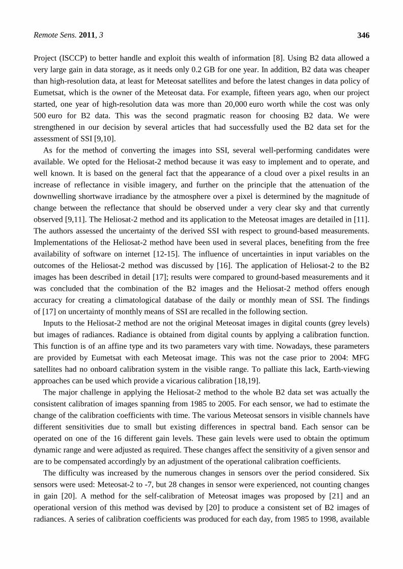
The Meteosat series of satellites are geostationary and provide synoptic views of Europe, Africa and
Atlantic Ocean for meteorological purposes. They are nominally located over the Gulf of Guinea at
longitudes close to 0°. Initiated by the European Space Agency, the program is currently operated by
Eumetsat, a European agency comprising the national weather offices. Only images taken in the visible
channel are dealt with in this paper. Such images clearly depict clouds and more generally the optical
state of the atmosphere (Figure 1). They are currently used to assess SSI with spatial and temporal
resolutions better than those in SRB.
Figure 1. Example of a Meteosat image in visible channel, taken on 7 September 2010, at
1200 UTC. Reflectance increases from black to white. The area covered is the same for
Meteosat First and Second Generations. (Copyright Eumetsat, 2010).
The HelioClim project is an initiative of MINES ParisTech launched in 1997, to increase knowledge
on SSI and to offer SSI values for any site, any instant over a large geographical area and long period
of time, to a wide audience [6]. It covers Europe, Africa and the Atlantic Ocean. The HelioClim-1
database, abbreviated in HC-1, offers daily values of SSI for the period 1985–2005. It has been created
from archives of images of the Meteosat First Generation (MFG). The HelioClim-3 database,

Remote Sens. 2011, 3
345
abbreviated to HC-3, represents a step forward regarding spatial and time resolution, clarifying
uncertainty on SSI, and time needed to access recent data. It exploits the enhanced capabilities of the
series of satellites Meteosat Second Generation (MSG) to deliver values of SSI every 15 min with a
spatial resolution of 3 km at nadir. To achieve this, MINES ParisTech acquired a MSG receiving
station in 2003 building upon its experience gained with the previous Meteosat satellites [7] and has
set up a routine operation for converting Meteosat data into SSI on a near-real time basis.
The main objectives of this article are to share this experience in building these two climatological
databases of SSI, to describe their construction, to discuss their quality and limitations, and to analyze
whether both databases can be combined to provide seamless time-series of daily and monthly means
of SSI spanning from 1985 to date.
We will first discuss the general challenges that we have encountered in the HelioClim project.
Then we will focus on those specific to the HC-1 database, how we solved them and our choice of a set
of Meteosat images in reduced resolution. We will describe the construction of the HC-1 database of
daily means of SSI by explaining the practical problems and their influence on the uncertainty of the
resulting SSI. We will show several examples of HC-1 time-series of monthly values and compare
them to existing ground-based measurements. These examples illustrate the performances and
limitations of the HC-1 database. Then, we will discuss the new challenge that we faced in 2003 with
the advent of the MSG series of satellites. We will describe the new HC-3 database and discuss also its
performances and limitations. We will analyze the concatenation of the two databases to create a
virtual single climatology and will study the consistency in time of this combination. Finally, we will
conclude on the HelioClim family of databases.
2. What Are the Challenges?
Creating a climatological database of SSI involves selecting: (i) a set of satellites images; (ii) a
method to process these images; and (iii) a tool for disseminating the data. All elements must be
consistent with each other: the method should be appropriate to the given images, the created database
should adapt to the dissemination tool. Each of the three elements is important; their combination is a
necessary condition for the climatology to exist and be exploited by users.
Of course, there are several constraints on any project. Usually, a project has limited resources in
skilled manpower, computer, storage and money. The HelioClim project was no exception. We tried to
find the best trade-off between the constraints, our ambitions and maintain scientific quality. As a
consequence, we have limited our own development of methods and tools. We opted for a set of
images in reduced resolution as input images, the Heliosat-2 method to convert these images into SSI,
and the SoDa Service for dissemination. These elements are discussed in the following.
One obstacle to the production of a climatological database is the large amount of data to process.
Considering the example of the MFG satellites, one third of the surface of the Earth was imaged every
half-hour with a pixel size of 2.5 km at nadir, yielding series of images of 5,000 × 5,000 pixels. Within
an image, approximately 30% of pixels are outside the Earth rim (Figure 1) and therefore offer no
interest for the computation of the SSI. Considering the remaining pixels, one year of data means
approximately a storage capacity of 243 GB. A set of Meteosat images in reduced spatial resolution,
called ISCCP-B2 data, B2 for short, was created for the International Satellite Cloud Climatology
Remote Sens. 2011, 3
346
Project (ISCCP) to better handle and exploit this wealth of information [8]. Using B2 data allowed a
very large gain in data storage, as it needs only 0.2 GB for one year. In addition, B2 data was cheaper
than high-resolution data, at least for Meteosat satellites and before the latest changes in data policy of
Eumetsat, which is the owner of the Meteosat data. For example, fifteen years ago, when our project
started, one year of high-resolution data was more than 20,000 euro worth while the cost was only
500 euro for B2 data. This was the second pragmatic reason for choosing B2 data. We were
strengthened in our decision by several articles that had successfully used the B2 data set for the
assessment of SSI [9,10].
As for the method of converting the images into SSI, several well-performing candidates were
available. We opted for the Heliosat-2 method because it was easy to implement and to operate, and
well known. It is based on the general fact that the appearance of a cloud over a pixel results in an
increase of reflectance in visible imagery, and further on the principle that the attenuation of the
downwelling shortwave irradiance by the atmosphere over a pixel is determined by the magnitude of
change between the reflectance that should be observed under a very clear sky and that currently
observed [9,11]. The Heliosat-2 method and its application to the Meteosat images are detailed in [11].
The authors assessed the uncertainty of the derived SSI with respect to ground-based measurements.
Implementations of the Heliosat-2 method have been used in several places, benefiting from the free
availability of software on internet [12-15]. The influence of uncertainties in input variables on the
outcomes of the Heliosat-2 method was discussed by [16]. The application of Heliosat-2 to the B2
images has been described in detail [17]; results were compared to ground-based measurements and it
was concluded that the combination of the B2 images and the Heliosat-2 method offers enough
accuracy for creating a climatological database of the daily or monthly mean of SSI. The findings
of [17] on uncertainty of monthly means of SSI are recalled in the following section.
Inputs to the Heliosat-2 method are not the original Meteosat images in digital counts (grey levels)
but images of radiances. Radiance is obtained from digital counts by applying a calibration function.
This function is of an affine type and its two parameters vary with time. Nowadays, these parameters
are provided by Eumetsat with each Meteosat image. This was not the case prior to 2004: MFG
satellites had no onboard calibration system in the visible range. To palliate this lack, Earth-viewing
approaches can be used which provide a vicarious calibration [18,19].
The major challenge in applying the Heliosat-2 method to the whole B2 data set was actually the
consistent calibration of images spanning from 1985 to 2005. For each sensor, we had to estimate the
change of the calibration coefficients with time. The various Meteosat sensors in visible channels have
different sensitivities due to small but existing differences in spectral band. Each sensor can be
operated on one of the 16 different gain levels. These gain levels were used to obtain the optimum
dynamic range and were adjusted as required. These changes affect the sensitivity of a given sensor and
are to be compensated accordingly by an adjustment of the operational calibration coefficients.
The difficulty was increased by the numerous changes in sensors over the period considered. Six
sensors were used: Meteosat-2 to -7, but 28 changes in sensor were experienced, not counting changes
in gain [20]. A method for the self-calibration of Meteosat images was proposed by [21] and an
operational version of this method was devised by [20] to produce a consistent set of B2 images of
radiances. A series of calibration coefficients was produced for each day, from 1985 to 1998, available
Remote Sens. 2011, 3
347
on internet. After that date, Eumetsat produced daily sets of coefficients. The similarity of the two
series of coefficients was demonstrated by [22] who concluded that a consistent time-series of images
of radiances can be created from 1985 to 2005 from the B2 images.
Finally, we opted for the SoDa Service (www.soda-is.com) as a means to disseminate the HelioClim
databases. This service was established in an operational way in 2003 [23] and is now widely used by
communities interested in solar radiation: more than 50,000 users in 2010. Data can be retrieved by
users using a standard internet browser. Therefore, by choosing this service, the HelioClim database
benefits from the notoriety of the SoDa Service.
3. The HelioClim-1 Database (HC-1)
The B2 data set was produced by Eumetsat from Meteosat images by first performing a time
sampling that reduced the frequency of observation to the standard meteorological synoptic 3-h
intervals, starting at 0000 UTC. This sampling is not time averaging; the first image available and of
good quality was selected to represent each 3-h interval. Secondly, the higher-resolution data in the
visible-channel were averaged to match the lower resolution of infrared-channel data (i.e., an image of
2,500 × 2,500 pixels with a resolution of 5 km). Finally, a spatial sampling was performed by taking
1 pixel over 6 in each direction, starting with the south-easternmost pixel.
The B2 data set spans from 1985 to 2005. It covers the whole field of view of Meteosat, i.e.,
Europe, Africa and the Atlantic Ocean. Meteosat data were converted into radiances as discussed
earlier. Each image of radiances was processed by the Heliosat-2 method, yielding an image of the
hourly mean of SSI. Then, the daily mean of SSI is computed from all images available for this day and
pixel. It is stored into the HC-1 database that comprises 118,500 B2 pixels.
The assessment of SSI for any geographical site is made by the means of a linear interpolator of
gravity-type applied to the nine nearest B2 pixels. After several comparisons with the nearest neighbor
and the geodetic distance, we selected the effective distance proposed by [24] and used by [25] for
mapping solar radiation climate in Africa. In a first approximation, one may consider that HC-1 has an
effective pixel of 30 km in size at nadir.
An application—more precisely, a web service—in the SoDa Service provides a time-series of SSI
for any site, and any period between 1 January 1985 and 31 December 2005. It performs the retrieval of
the time-series for each of the nine nearest B2 pixels and their interpolation in space. This service also
performs the temporal aggregation of the data: one can ask for daily or monthly means of SSI. The
initial version of the HC-1 database was released in 2003. Several corrections were necessary. One
major drawback was due to errors in navigation in original Meteosat images and was discovered in
January 2005. The HC-1 database was then reconstructed and the current version HC-1v4 has been
available since March 2006.
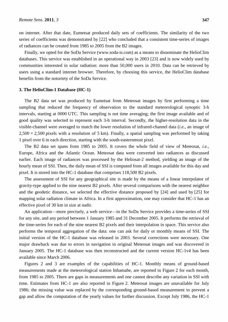
Figures 2 and 3 are examples of the capabilities of HC-1. Monthly means of ground-based
measurements made at the meteorological station Inhamabe, are reported in Figure 2 for each month,
from 1985 to 2005. There are gaps in measurements and one cannot describe any variation in SSI with
time. Estimates from HC-1 are also reported in Figure 2. Meteosat images are unavailable for July
1986; the missing value was replaced by the corresponding ground-based measurement to prevent a
gap and allow the computation of the yearly values for further discussion. Except July 1986, the HC-1
Remote Sens. 2011, 3
348
time-series is complete. One notes visually that the agreement of HC-1 with the actual measurements is
fairly good. HC-1 can be used to provide a first description of the change in SSI over the 21 year
period, thus palliating gaps in ground-based measurements. If an accurate sort of calibration function
can be found between existing HC-1 values and measurements, then HC-1 values can be transformed
into an accurate and complete time-series reproducing the measurements.
Figure 2. Monthly means of SSI from HC-1 in Inhamabe during the period 1985–2005 and
comparison with the available ground-based measurements (WRDC).
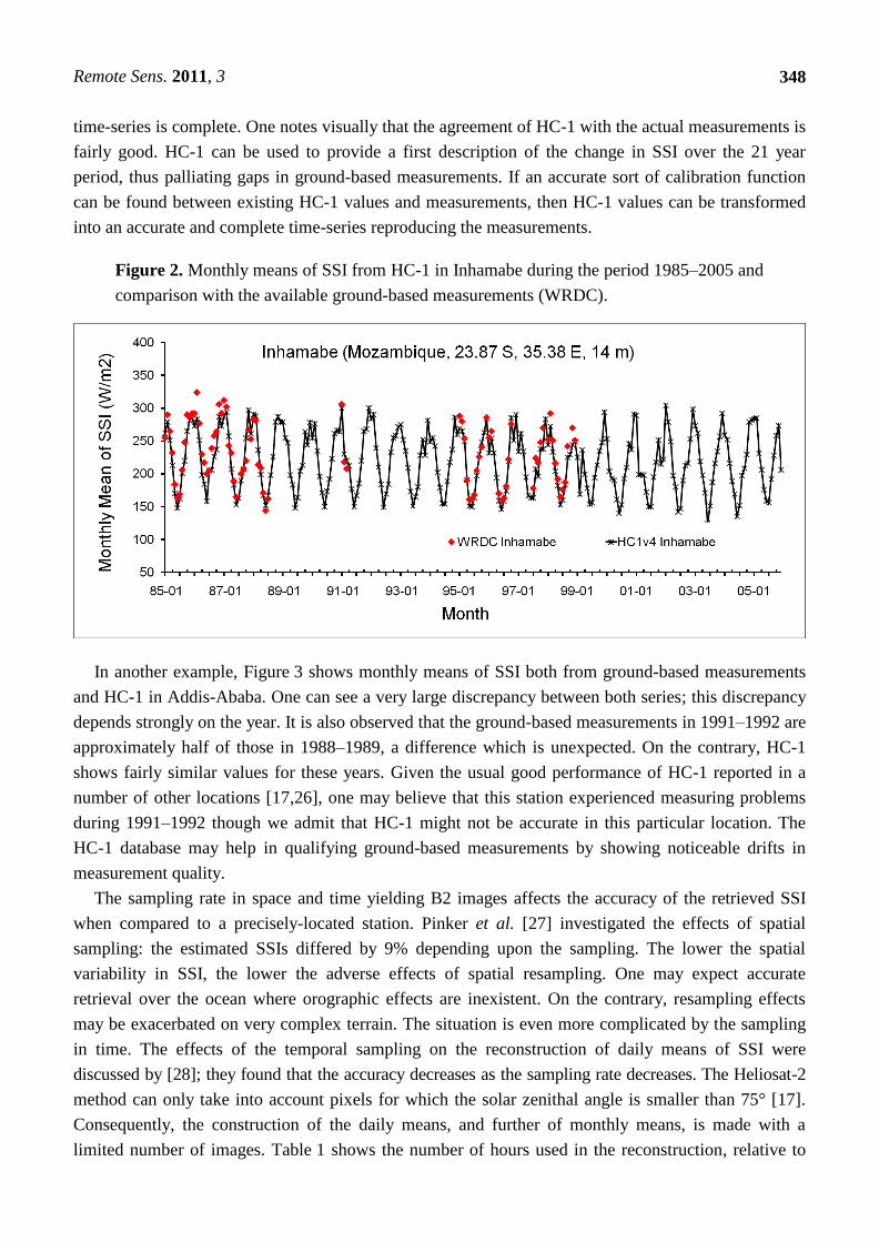
In another example, Figure 3 shows monthly means of SSI both from ground-based measurements
and HC-1 in Addis-Ababa. One can see a very large discrepancy between both series; this discrepancy
depends strongly on the year. It is also observed that the ground-based measurements in 1991–1992 are
approximately half of those in 1988–1989, a difference which is unexpected. On the contrary, HC-1
shows fairly similar values for these years. Given the usual good performance of HC-1 reported in a
number of other locations [17,26], one may believe that this station experienced measuring problems
during 1991–1992 though we admit that HC-1 might not be accurate in this particular location. The
HC-1 database may help in qualifying ground-based measurements by showing noticeable drifts in
measurement quality.
The sampling rate in space and time yielding B2 images affects the accuracy of the retrieved SSI
when compared to a precisely-located station. Pinker et al. [27] investigated the effects of spatial
sampling: the estimated SSIs differed by 9% depending upon the sampling. The lower the spatial
variability in SSI, the lower the adverse effects of spatial resampling. One may expect accurate
retrieval over the ocean where orographic effects are inexistent. On the contrary, resampling effects
may be exacerbated on very complex terrain. The situation is even more complicated by the sampling
in time. The effects of the temporal sampling on the reconstruction of daily means of SSI were
discussed by [28]; they found that the accuracy decreases as the sampling rate decreases. The Heliosat-2
method can only take into account pixels for which the solar zenithal angle is smaller than 75° [17].
Consequently, the construction of the daily means, and further of monthly means, is made with a
limited number of images. Table 1 shows the number of hours used in the reconstruction, relative to
Remote Sens. 2011, 3
349
the day length in hours, for longitude 0 and various latitudes. This number does not vary significantly
with longitude, except for those close to the borders of the Meteosat field-of-view.
Figure 3. Monthly means of SSI from HC-1 in Addis-Ababa during the period 1985–2005
and comparison with the available ground-based measurements (WRDC).
Table 1. Relative percentage of hours used in the construction of daily means of SSI in
HC-1, knowing that maximum is 33% for B2 data set.
Latitude (deg.) 60 (−60) 55 (−55) 45 (−45) 35 (−35) 25 (−25) 15 (−15) 0
Rel. number min (winter) 0 0 14 21 24 24 24
Rel. number max (summer) 16 30 30 30 31 33 33
During winter, the sun is low above the horizon in middle to large latitudes and the day length is
short. Therefore, the chance to have many observations with solar zenithal angle less than 75° are small
and the number of available hours is the lowest. The opposite occurs in summer. Nevertheless, one can
see that, at most, only one-third of the hours can be used to assess the daily value: in all cases, the
number of hours is not enough to describe complex highly-variable situations. Therefore, one may
expect large discrepancies between HC-1 retrievals and actual SSIs.
In addition, the instants of sampling are defined in UTC—every 3 h—and are the same for all
pixels. The few available hours are not necessarily well distributed with respect to the sun course and
irradiance profile. It may well be that a specific climate is misrepresented. For example, given a month,
if clouds occur frequently in the morning only, and if the one or two available B2 observations are
made in the afternoon, then the month will be considered as most often clear. Other examples can be
found where the rate and instants of sampling are inadequate to describe the cloud cover and therefore
lead to inaccurate estimated SSI.
As a conclusion, one should be cautious in using HC-1 in high latitudes and in any case where the
variability in SSI with respect to space and time is large for scales of order of 10 km and 1 h, apart
from the variability induced by the sun course.

Remote Sens. 2011, 3
350
4. Quality and Limitations of HC-1
To our knowledge, two articles have been published assessing the uncertainty of the daily and
monthly means of SSI provided by HC-1 [17,26]. In both cases, this was done by comparing HC-1
values to ground-based measurements. The authors follow the ISO standard [29]: they compute the
difference: estimated-measured for each day, and summarize these differences by the bias, the root
mean square difference (RMSD) and the correlation coefficient.
It should be recalled that the two time-series to compare are different in nature: one is made of
pin-pointed time-integrated measurements, the other of space-averaged instantaneous assessments.
Accordingly, a discrepancy is expected because of the natural variability of SSI in space; [3] found a
standard deviation of 10–15% within a pixel relative to the hourly mean of SSI. Though it is difficult to
predict because spatial variability is not a random variable, we can expect a discrepancy of a few
percent relative to the monthly mean of SSI.
Lefèvre et al. [17] used measurements for 55 sites in Europe covering July 1994 to June 1995, and
35 sites in Africa spanning over 48 months from January 1994 to December 1997. Their results of
monthly means are reported in Table 2. The authors showed that their results are in accordance with
those obtained by [5] with the NASA-SRB data set. Studying 11 stations in North Africa, [26] found
similar performances between HC-1 and NASA-SRB.
Table 2. Comparison between HC-1 and ground-based measurements of monthly mean of
SSI (in W/m2) [17]. RMSD: root mean square difference. In brackets, quantities are relative
to the mean measured SSI.
Period
Number of
observations
(months)
Mean SSI
(measured)
Bias
(relative)
RMSD
(relative)
Correlation
coefficient
Europe 1994 172 147 −6 (−4%) 17 (12%) 0.97
Europe 1995 462 149 −14 (−9%) 24 (16%) 0.95
Africa 1994 280 228 −1 (0%) 24 (11%) 0.92
Africa 1995 322 224 5 (2%) 24 (11%) 0.92
Africa 1996 310 218 7 (3%) 27 (12%) 0.90
Africa 1997 269 219 8 (4%) 29 (13%) 0.90
Considering the quality of HC-1 (Table 2), Lefèvre et al. [17] concluded that a climatology of the
SSI can be constructed from B2 data set. However, they underlined that the quality may vary strongly
from one site to another.
We now examine their conclusions for a limited number of sites but over a longer period. We aim at
providing further evidence on the capabilities of HC-1 for climate applications and detailing its
limitations. Thanks to the World Radiation Data Center (WRDC), the Egyptian Meteorological
Authority and Meteo-France, we have assembled monthly values measured by meteorological
networks. Eleven stations were selected because they offer long time-series of monthly
values—greater than 97 months—and cover major climatic areas (Table 3). The approximate size of
the pixel in HC-1 and HC-3 is reported for each site in this table.
Remote Sens. 2011, 3
351
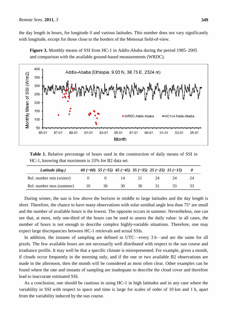
For Europe, we used more stations than the six shown in Table 3; we present here those that best
illustrate the quality and limitations of HC-1. Arguably, we have selected two stations in France:
Carpentras and Nice, which are geographically close, approximately 300 km apart, and experience
approximately the same sunny climate in the Provence. We expect a similar performance from HC-1
for these sites and we will discuss this further.
Table 3. Ground-measuring stations used for comparison.
Station name WMO ID Latitude
(°)
Longitude
(°)
Altitude
(m)
Pixel size HC-1
and HC-3 (km) Country
Helsinki 29740 60.32 24.97 51 80, 8 Finland
Eskadalemuir 31620 55.32 −3.2 242 80, 8 UK
Vienna 110350 48.25 16.37 203 50, 5 Austria
Payerne 66100 46.82 6.95 490 50, 5 Switzerland
Carpentras 75860 44.07 5.05 106 50, 5 France
Nice 76900 43.65 7.20 4 50, 5 France
Sidi Bou Said 36.87 10.23 127 40, 4 Tunisia
Aswan 624140 23.97 32.78 192 40, 4 Egypt
Tamanrasset 60680 22.78 5.52 1377 35, 4 Algeria
Bulawayo 679640 −20.15 28.62 1343 40, 4 Zimbabwe
Inhamabe 67323 −23.87 35.38 14 40, 4 Mozambique
Five stations are in Africa. We would have been happy to have dealt with more stations, such as those
used by Diabaté et al. [25] who define 20 solar radiation climates in Africa, but we stress here the
difficulty in finding reliable long time-series of SSI measured by meteorological stations, and we
acknowledge the work done by the meteorological networks and WRDC. The measurements taken at
these African stations have already been compared to HC-1 for different time periods [17,26]. These
published results will guide our own analyses.
Table 4 reports on the comparison between these measurements and the SSI from HC-1. The
correlation coefficient is large in all cases: greater than 0.9. The month-to-month variations are well
reproduced for each site.
Considering the relative bias and the RMSD, Table 4 can be split in two parts: the northernmost
stations: Helsinki, Eskadalemuir, Vienna and Payerne, and the others. The northernmost sites exhibit
large and negative bias (underestimation). The fact that the bias is larger, in absolute and relative
values, than for sites located at lower latitudes is likely due to the poor number of images used to
compute the daily means, especially in winter (Table 1). This is substantiated by a similar analysis
made for three other stations at approximately 60°N, eight in Germany and one in Austria, for the same
period: relative bias was negative and as large as in Table 4. This is also in agreement with Table 2.
We conclude that HC-1 underestimates SSI because of the sampling rate in time of the B2 images. As
a first guess, sites of latitudes greater than 45°, and most likely less than −45°, experience
underestimation by HC-1. This conclusion may nevertheless be contradicted by local conditions, as
previously discussed.
Remote Sens. 2011, 3
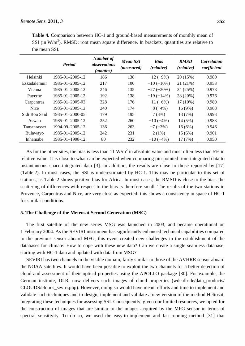
352
Table 4. Comparison between HC-1 and ground-based measurements of monthly mean of
SSI (in W/m2). RMSD: root mean square difference. In brackets, quantities are relative to
the mean SSI.
Period
Number of
observations
(months)
Mean SSI
(measured)
Bias
(relative)
RMSD
(relative)
Correlation
coefficient
Helsinki 1985-01–2005-12 186 138 −12 (−9%) 20 (15%) 0.980
Eskadalemuir 1985-01–2005-12 217 100 −10 (−10%) 21 (21%) 0.953
Vienna 1985-01–2005-12 246 135 −27 (−20%) 34 (25%) 0.978
Payerne 1985-01–2005-12 192 138 −19 (−14%) 28 (20%) 0.976
Carpentras 1985-01–2005-02 228 176 −11 (−6%) 17 (10%) 0.989
Nice 1985-01–2005-12 240 174 −8 (−4%) 16 (9%) 0.988
Sidi Bou Said 1985-01–2000-05 179 195 7 (3%) 13 (7%) 0.993
Aswan 1985-01–2005-12 252 260 −10 (−4%) 14 (5%) 0.983
Tamanrasset 1994-09–2005-12 136 263 −7 (−3%) 16 (6%) 0.946
Bulawayo 1985-01–2005-12 242 231 2 (1%) 15 (6%) 0.901
Inhamabe 1985-01–1998-12 80 232 −10 (−4%) 17 (7%) 0.950
As for the other sites, the bias is less than 11 W/m2 in absolute value and most often less than 5% in
relative value. It is close to what can be expected when comparing pin-pointed time-integrated data to
instantaneous space-integrated data [3]. In addition, the results are close to those reported by [17]
(Table 2). In most cases, the SSI is underestimated by HC-1. This may be particular to this set of
stations, as Table 2 shows positive bias for Africa. In most cases, the RMSD is close to the bias: the
scattering of differences with respect to the bias is therefore small. The results of the two stations in
Provence, Carpentras and Nice, are very close as expected: this shows a consistency in space of HC-1
for similar conditions.
5. The Challenge of the Meteosat Second Generation (MSG)
The first satellite of the new series MSG was launched in 2003, and became operational on
1 February 2004. As the SEVIRI instrument has significantly enhanced technical capabilities compared
to the previous sensor aboard MFG, this event created new challenges in the establishment of the
databases for climate: How to cope with these new data? Can we create a single seamless database,
starting with HC-1 data and updated with data from MSG?
SEVIRI has two channels in the visible domain, fairly similar to those of the AVHRR sensor aboard
the NOAA satellites. It would have been possible to exploit the two channels for a better detection of
cloud and assessment of their optical properties using the APOLLO package [30]. For example, the
German institute, DLR, now delivers such images of cloud properties (wdc.dlr.de/data_products/
CLOUDS/clouds_seviri.php). However, doing so would have meant efforts and time to implement and
validate such techniques and to design, implement and validate a new version of the method Heliosat,
integrating these techniques for assessing SSI. Consequently, given our limited resources, we opted for
the construction of images that are similar to the images acquired by the MFG sensor in terms of
spectral sensitivity. To do so, we used the easy-to-implement and fast-running method [31] that
Remote Sens. 2011, 3
353
combines the radiances of the two narrow visible bands of SEVIRI to produce broadband radiances
that are almost identical to those observed in the broadband channel of Meteosat-7, the last satellite of
the MFG series.
Contrary to MFG, receiving stations for the high-quality signal are cheap and we were able to afford
one. Simultaneously, costs of computers and storage capacities were decreasing; therefore, we were
able to process and store a large amount of data unlike six years earlier. Since 1 February 2004, we
have been acquiring images every 15 min with a pixel of 3 km in size at nadir. Meteosat images are
converted into radiances using the calibration coefficients embedded in each image. Each image of
radiances is then processed by the Heliosat-2 method and yields an image of the 15-min mean of SSI. It
is stored in the HC-3 database which comprises approximately nine million pixels. Unlike HC-1,
post-processing is applied to the 15 min outputs from the Heliosat-2 method in order to decrease the
overestimation observed for low SSI and the underestimation observed for large SSI. The effect of this
post-processing on monthly or yearly means is difficult to predict as it is applied on 15 min values and
depends on the SSI itself. As a first approximation, the post-processing yields an increase of
approximately 10 W/m2 (approximately 3% in relative value) at very sunny sites exhibiting very large
SSI all year round, such as in Tamanrasset or Aswan. The daily mean of SSI was computed for all
images available for this day and pixel.
Like HC-1, a web service in the SoDa Service provides a time-series of SSI for any site, and any
period, starting from 1 February 2004. This service performs the temporal aggregation of the data. It is
important to note that SSI values supplied by the HC-3 database are for the pixel containing the
requested site with the correction of altitude of this particular site relative to the mean altitude of the
Meteosat pixel [26]. There is no spatial average at all, following [11]. The current version HC-3v2 was
made available in June 2009. It corrected drawbacks observed in the initial version over African
deserts and includes altitude correction.
The HC-3 database has gone through extensive validation of 15 min and hourly values. However,
no article has yet been published on this validation, though the results for 29 sites—26 in Europe, one
in the Middle East, one in North Africa, one in South Africa—are published on the SoDa Service
(www.soda-is.com/eng/help/helioclim3_uncertainty_eng.html). These results are of interest here as the
bias observed in hourly values should be close to that observed for daily and monthly values because it
is a systematic error. These results are referred to as SoDa validation results hereafter and will guide
our analysis.
Table 5 reports the results of the comparison between the monthly means of SSI measured at the
stations listed in Table 3—except Sidi Bou Said which has no data for this period—and those from
HC-3. The correlation coefficient is large in all cases; i.e., greater than 0.9, and in several cases greater
than 0.99. This means that the month-to-month variations in SSI are well reproduced by the HC-3
database. If we exclude the two stations Bulawayo and Inhamabe, one notes that results are very
similar for all sites though they are located in very different climates, spanning from 23° to 60°. This is
a very satisfactory result which demonstrates the consistency in space of the quality of HC-3. The
SoDa validation results confirm this observation.
Remote Sens. 2011, 3
354
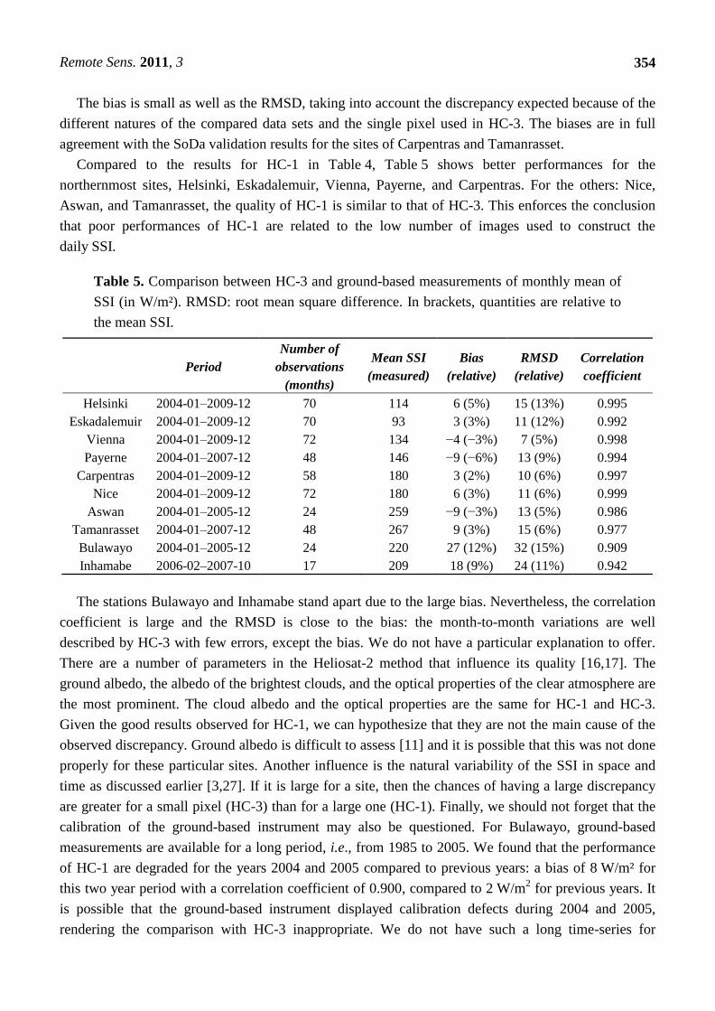
The bias is small as well as the RMSD, taking into account the discrepancy expected because of the
different natures of the compared data sets and the single pixel used in HC-3. The biases are in full
agreement with the SoDa validation results for the sites of Carpentras and Tamanrasset.
Compared to the results for HC-1 in Table 4, Table 5 shows better performances for the
northernmost sites, Helsinki, Eskadalemuir, Vienna, Payerne, and Carpentras. For the others: Nice,
Aswan, and Tamanrasset, the quality of HC-1 is similar to that of HC-3. This enforces the conclusion
that poor performances of HC-1 are related to the low number of images used to construct the
daily SSI.
Table 5. Comparison between HC-3 and ground-based measurements of monthly mean of
SSI (in W/m²). RMSD: root mean square difference. In brackets, quantities are relative to
the mean SSI.
Period
Number of
observations
(months)
Mean SSI
(measured)
Bias
(relative)
RMSD
(relative)
Correlation
coefficient
Helsinki 2004-01–2009-12 70 114 6 (5%) 15 (13%) 0.995
Eskadalemuir 2004-01–2009-12 70 93 3 (3%) 11 (12%) 0.992
Vienna 2004-01–2009-12 72 134 −4 (−3%) 7 (5%) 0.998
Payerne 2004-01–2007-12 48 146 −9 (−6%) 13 (9%) 0.994
Carpentras 2004-01–2009-12 58 180 3 (2%) 10 (6%) 0.997
Nice 2004-01–2009-12 72 180 6 (3%) 11 (6%) 0.999
Aswan 2004-01–2005-12 24 259 −9 (−3%) 13 (5%) 0.986
Tamanrasset 2004-01–2007-12 48 267 9 (3%) 15 (6%) 0.977
Bulawayo 2004-01–2005-12 24 220 27 (12%) 32 (15%) 0.909
Inhamabe 2006-02–2007-10 17 209 18 (9%) 24 (11%) 0.942
The stations Bulawayo and Inhamabe stand apart due to the large bias. Nevertheless, the correlation
coefficient is large and the RMSD is close to the bias: the month-to-month variations are well
described by HC-3 with few errors, except the bias. We do not have a particular explanation to offer.
There are a number of parameters in the Heliosat-2 method that influence its quality [16,17]. The
ground albedo, the albedo of the brightest clouds, and the optical properties of the clear atmosphere are
the most prominent. The cloud albedo and the optical properties are the same for HC-1 and HC-3.
Given the good results observed for HC-1, we can hypothesize that they are not the main cause of the
observed discrepancy. Ground albedo is difficult to assess [11] and it is possible that this was not done
properly for these particular sites. Another influence is the natural variability of the SSI in space and
time as discussed earlier [3,27]. If it is large for a site, then the chances of having a large discrepancy
are greater for a small pixel (HC-3) than for a large one (HC-1). Finally, we should not forget that the
calibration of the ground-based instrument may also be questioned. For Bulawayo, ground-based
measurements are available for a long period, i.e., from 1985 to 2005. We found that the performance
of HC-1 are degraded for the years 2004 and 2005 compared to previous years: a bias of 8 W/m² for
this two year period with a correlation coefficient of 0.900, compared to 2 W/m2 for previous years. It
is possible that the ground-based instrument displayed calibration defects during 2004 and 2005,
rendering the comparison with HC-3 inappropriate. We do not have such a long time-series for
Remote Sens. 2011, 3
355
Inhamabe and could not perform a similar study. However, we found that for 2004 and 2005, the
difference between HC-3 and HC-1 is 10 W/m2. If we combine this with the results of HC-1 for
Inhamabe (−10 W/m2, Table 4), we can expect a bias between HC-3 and ground-based measurements
close to 0. This only partly explains the observed bias and it is possible that the station Inhamabe
experienced drawbacks in its measurements. Our belief is substantiated by the low relative bias (3%)
found in the SoDa validation results for the station De Aar in South Africa, whose latitude and
longitude are −30.66° and 23.99°.
6. Merging HC-1 and HC-3
We have shown that both HC-1 and HC-3 provided accurate time-series of SSI in their respective
periods. Now, we faced a new challenge: can we create a single time-series out of the two databases,
spanning from 1985 till now, and offering a consistent description of SSI with time?
Practically, this can be done by creating a first time-series from the HC-1 database, and then by
augmenting it by adding the time-series from the HC-3 database. However, when concatenating the
time-series, we are merging two data sets of different spatial properties which could create a jump in a
time-series of SSI that is solely due to the change in spatial resolution at the junction of the two data
sets [27]. The magnitude of the jump would depend on the actual underlying spatial variability of the
SSI. The lower this variability, the lower the magnitude of the jump would be. In addition, as already
discussed, the resampling in time of the B2 images induces limitations in the description of the daily
mean of SSI. An additional jump would be created by this effect, whose magnitude depends on the
temporal variability of the SSI [28]. Finally, the images, their calibration and their processing and
post-processing, slightly differ between HC-1 and HC-3 which induces a difference in retrieved SSI.
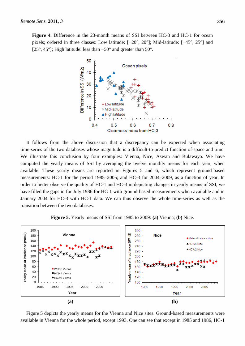
To better understand the change in SSI due to the low number of images used to construct the daily
means in HC-1, we studied the difference between HC-3 and HC-1 over the ocean for different
latitudes. One can expect the spatial variability to be low over the ocean; studying only ocean pixels
should enable us to mostly focus on the effects of the temporal resampling. HC-1 and HC-3 values
were extracted for a few pixels over the ocean. We have computed the mean difference between HC-3
and HC-1 for the 23 common months in 2004 and 2005. To study the influence of the type of sky, we
have also divided the HC-3 SSI by the corresponding irradiance at the top-of-atmosphere, yielding the
clearness index, ranging from 0.4 (cloudy sky) to approximately 0.7 (clear sky). The differences in SSI
for all pixels are ordered in three classes of latitudes and drawn as a function of the HC-3 clearness
index (Figure 4). One can see that the difference between HC-3 and HC-1 has a tendency to increase
with the absolute value of the latitude: this corresponds to the decreasing number of images available
to construct the daily means. The difference decreases as the clearness index increases: it means that
for a given range of latitude, the error due to the small number of images is smaller in case of clear
skies. The difference ranges between 5 W/m² and 40 W/m² found at latitude 55°. The analysis of the
values reveals that the difference between HC-3 and HC-1 is approximately symmetrical between the
Northern and Southern hemispheres. The lowest values (~10 W/m2, ~3% in relative value) are the
typical difference that one can expect between HC-3 and HC-1, as a result of the differences in input
images, calibration and processing.
Remote Sens. 2011, 3
356
Figure 4. Difference in the 23-month means of SSI between HC-3 and HC-1 for ocean
pixels; ordered in three classes: Low latitude: [−20°, 20°]; Mid-latitude: [−45°, 25°] and
[25°, 45°]; High latitude: less than −50° and greater than 50°.
It follows from the above discussion that a discrepancy can be expected when associating
time-series of the two databases whose magnitude is a difficult-to-predict function of space and time.
We illustrate this conclusion by four examples: Vienna, Nice, Aswan and Bulawayo. We have
computed the yearly means of SSI by averaging the twelve monthly means for each year, when
available. These yearly means are reported in Figures 5 and 6, which represent ground-based
measurements: HC-1 for the period 1985–2005; and HC-3 for 2004–2009, as a function of year. In
order to better observe the quality of HC-1 and HC-3 in depicting changes in yearly means of SSI, we
have filled the gaps in for July 1986 for HC-1 with ground-based measurements when available and in
January 2004 for HC-3 with HC-1 data. We can thus observe the whole time-series as well as the
transition between the two databases.
Figure 5. Yearly means of SSI from 1985 to 2009: (a) Vienna; (b) Nice.
0
20
40
60
80
100
120
140
160
180
200
1985 1990 1995 2000 2005
Ye
arl
y m
ea
n o
f ir
rad
ian
ce
(W
/m2
)
Year
Vienna
WRDC Vienna
HC1v4 Vienna
HC3v2 Vienna
(a) (b)
Figure 5 depicts the yearly means for the Vienna and Nice sites. Ground-based measurements were
available in Vienna for the whole period, except 1993. One can see that except in 1985 and 1986, HC-1
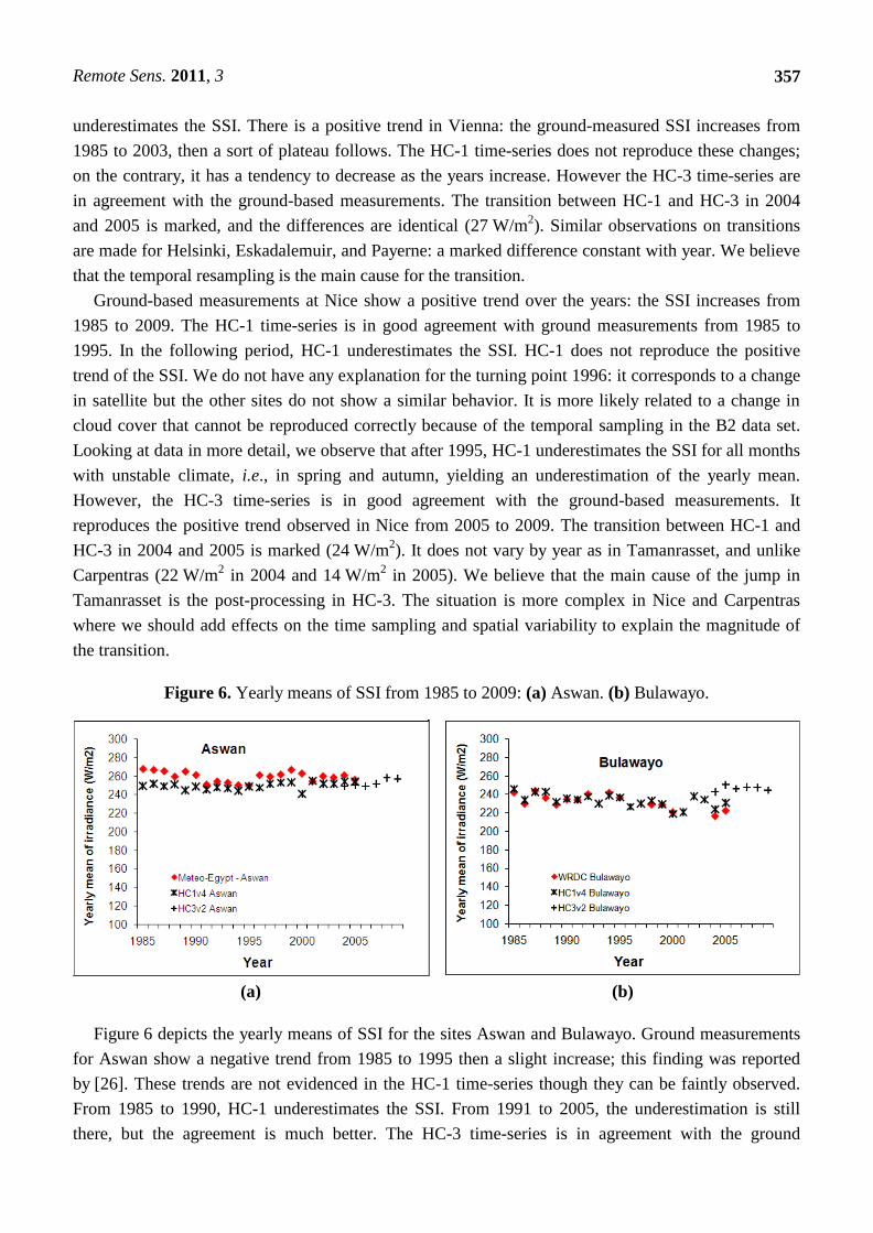
Remote Sens. 2011, 3
357
underestimates the SSI. There is a positive trend in Vienna: the ground-measured SSI increases from
1985 to 2003, then a sort of plateau follows. The HC-1 time-series does not reproduce these changes;
on the contrary, it has a tendency to decrease as the years increase. However the HC-3 time-series are
in agreement with the ground-based measurements. The transition between HC-1 and HC-3 in 2004
and 2005 is marked, and the differences are identical (27 W/m2). Similar observations on transitions
are made for Helsinki, Eskadalemuir, and Payerne: a marked difference constant with year. We believe
that the temporal resampling is the main cause for the transition.
Ground-based measurements at Nice show a positive trend over the years: the SSI increases from
1985 to 2009. The HC-1 time-series is in good agreement with ground measurements from 1985 to
1995. In the following period, HC-1 underestimates the SSI. HC-1 does not reproduce the positive
trend of the SSI. We do not have any explanation for the turning point 1996: it corresponds to a change
in satellite but the other sites do not show a similar behavior. It is more likely related to a change in
cloud cover that cannot be reproduced correctly because of the temporal sampling in the B2 data set.
Looking at data in more detail, we observe that after 1995, HC-1 underestimates the SSI for all months
with unstable climate, i.e., in spring and autumn, yielding an underestimation of the yearly mean.
However, the HC-3 time-series is in good agreement with the ground-based measurements. It
reproduces the positive trend observed in Nice from 2005 to 2009. The transition between HC-1 and
HC-3 in 2004 and 2005 is marked (24 W/m2). It does not vary by year as in Tamanrasset, and unlike
Carpentras (22 W/m2 in 2004 and 14 W/m
2 in 2005). We believe that the main cause of the jump in
Tamanrasset is the post-processing in HC-3. The situation is more complex in Nice and Carpentras
where we should add effects on the time sampling and spatial variability to explain the magnitude of
the transition.
Figure 6. Yearly means of SSI from 1985 to 2009: (a) Aswan. (b) Bulawayo.
(a) (b)
Figure 6 depicts the yearly means of SSI for the sites Aswan and Bulawayo. Ground measurements
for Aswan show a negative trend from 1985 to 1995 then a slight increase; this finding was reported
by [26]. These trends are not evidenced in the HC-1 time-series though they can be faintly observed.
From 1985 to 1990, HC-1 underestimates the SSI. From 1991 to 2005, the underestimation is still
there, but the agreement is much better. The HC-3 time-series is in agreement with the ground
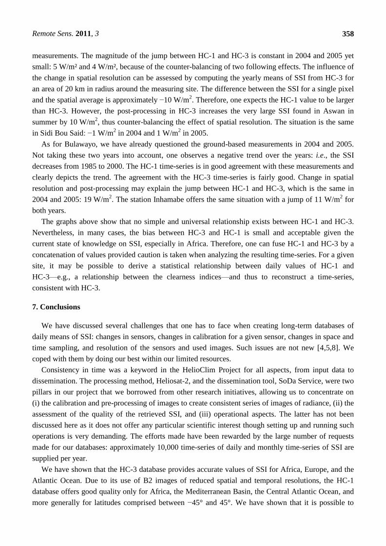
Remote Sens. 2011, 3
358
measurements. The magnitude of the jump between HC-1 and HC-3 is constant in 2004 and 2005 yet
small: 5 W/m² and 4 W/m², because of the counter-balancing of two following effects. The influence of
the change in spatial resolution can be assessed by computing the yearly means of SSI from HC-3 for
an area of 20 km in radius around the measuring site. The difference between the SSI for a single pixel
and the spatial average is approximately −10 W/m2. Therefore, one expects the HC-1 value to be larger
than HC-3. However, the post-processing in HC-3 increases the very large SSI found in Aswan in
summer by 10 W/m2, thus counter-balancing the effect of spatial resolution. The situation is the same
in Sidi Bou Said: −1 W/m2 in 2004 and 1 W/m
2 in 2005.
As for Bulawayo, we have already questioned the ground-based measurements in 2004 and 2005.
Not taking these two years into account, one observes a negative trend over the years: i.e., the SSI
decreases from 1985 to 2000. The HC-1 time-series is in good agreement with these measurements and
clearly depicts the trend. The agreement with the HC-3 time-series is fairly good. Change in spatial
resolution and post-processing may explain the jump between HC-1 and HC-3, which is the same in
2004 and 2005: 19 W/m2. The station Inhamabe offers the same situation with a jump of 11 W/m
2 for
both years.
The graphs above show that no simple and universal relationship exists between HC-1 and HC-3.
Nevertheless, in many cases, the bias between HC-3 and HC-1 is small and acceptable given the
current state of knowledge on SSI, especially in Africa. Therefore, one can fuse HC-1 and HC-3 by a
concatenation of values provided caution is taken when analyzing the resulting time-series. For a given
site, it may be possible to derive a statistical relationship between daily values of HC-1 and
HC-3—e.g., a relationship between the clearness indices—and thus to reconstruct a time-series,
consistent with HC-3.
7. Conclusions
We have discussed several challenges that one has to face when creating long-term databases of
daily means of SSI: changes in sensors, changes in calibration for a given sensor, changes in space and
time sampling, and resolution of the sensors and used images. Such issues are not new [4,5,8]. We
coped with them by doing our best within our limited resources.
Consistency in time was a keyword in the HelioClim Project for all aspects, from input data to
dissemination. The processing method, Heliosat-2, and the dissemination tool, SoDa Service, were two
pillars in our project that we borrowed from other research initiatives, allowing us to concentrate on
(i) the calibration and pre-processing of images to create consistent series of images of radiance, (ii) the
assessment of the quality of the retrieved SSI, and (iii) operational aspects. The latter has not been
discussed here as it does not offer any particular scientific interest though setting up and running such
operations is very demanding. The efforts made have been rewarded by the large number of requests
made for our databases: approximately 10,000 time-series of daily and monthly time-series of SSI are
supplied per year.
We have shown that the HC-3 database provides accurate values of SSI for Africa, Europe, and the
Atlantic Ocean. Due to its use of B2 images of reduced spatial and temporal resolutions, the HC-1
database offers good quality only for Africa, the Mediterranean Basin, the Central Atlantic Ocean, and
more generally for latitudes comprised between −45° and 45°. We have shown that it is possible to
Remote Sens. 2011, 3
359
easily construct time-series of daily, monthly or yearly means of SSI, from 1985 up to date. However,
caution should be taken in the analysis of such time-series, as the difference in processing, spatial and
temporal resolutions, between HC-1 and HC-3, may lead to a jump between the period covered by
HC-1 (1985–2005) and that of HC-3 (since 2004). The common period (2004–2005) may help in
detecting such cases.
Even if uncertainty is currently too great for accurate analyses of climate, the availability of these
time-series for virtually any location in the field-of-view of the Meteosat satellites should help any
community interested in climate applications to perform steps towards a better knowledge of the SSI
and its variation over recent years.
Acknowledgements
The authors are grateful to Eumetsat and Meteo-France for the provision of Meteosat data, the
World Radiation Data Center for supplying SSI data for ground measuring stations. Data for Aswan,
Carpentras and Nice, was kindly supplied by the Egyptian Meteorological Authority, and Meteo-France
respectively. We thank these institutes. The authors thank the company Transvalor which is taking care
of the SoDa Service for the common good, therefore permitting an efficient access to HelioClim
databases. The authors thank Thierry Ranchin for his help in clarifying the content of the article. The
research leading to these results has partly received funding from the European Union’s Seventh
Framework Programme (FP7/2007-2013) under Grant Agreement no. 218793 (MACC project).
References and Notes
1. Global Climate Observing System (GCOS) Essential Climate Variables. Available online:
www.wmo.int/pages/prog/gcos/index.php?name=EssentialClimateVariables (accessed on 16
February 2011).
2. Perez, R.; Seals, R.; Zelenka, A. Comparing satellite remote sensing and ground network
measurements for the production of site/time specific irradiance data. Solar Energy 1997, 60,
89-96.
3. Zelenka, A.; Perez, R.; Seals, R.; Renné, D. Effective accuracy of satellite-derived hourly
irradiances. Theor. Appl. Climatol. 1999, 62, 199-207.
4. Whitlock, C.H.; Charlock, T.P.; Staylor, W.F.; Pinker, R.T.; Laszlo, I.; Ohmura, A.; Gilgen, H.;
Konzelman, T.; DiPasquale, R.C.; Moats, C.D.; LeCroy, S.R.; Ritchey, N.A. First global WCRP
shortwave surface radiation budget dataset. Bull. Amer. Meteorol. Soc. 1995, 76, 905-922.
5. Darnell, W.L.; Staylor, W.F.; Ritchey, N.A.; Gupta, S.K.; Wilber, A.C. Surface radiation budget:
A long-term global dataset of shortwave and longwave fluxes. Eos Trans. AGU 27 February 1996.
6. Rigollier, C.; Wald, L. The HelioClim Project: From Satellite Images to Solar Radiation Maps. In
Proceedings of the ISES Solar World Congress 1999, Jerusalem, Israel, 4–9 July 1999; Volume I,
pp. 427-431.
7. Diabaté, L.; Moussu, G.; Wald, L. Description of an operational tool for determining global solar
radiation at ground using geostationary satellite images. Solar Energy 1989, 42, 201-207.
8. Schiffer, R.; Rossow, W.B. ISCCP global radiance data set: A new resource for climate research.
Bull. Amer. Meteorol. Soc. 1985, 66, 1498-1503.
Remote Sens. 2011, 3
360
9. Raschke, E.; Gratzki, A.; Rieland, M. Estimates of global radiation at the ground from the reduced
data sets of the International Satellite Cloud Climatology Project. J. Climate 1987, 7, 205-213.
10. Ba, M.; Nicholson, S.; Frouin, R. Satellite-derived surface radiation budget over the African
continent. Part II: Climatologies of the various components. J. Climate 2001, 14, 60-76.
11. Rigollier, C.; Lefèvre, M.; Wald, L. The method Heliosat-2 for deriving shortwave solar radiation
from satellite images. Solar Energy 2004, 77, 159-169.
12. Posselt, R.; Müller, R.; Trentmann, J.; Stöckli, R. Surface radiation climatology derived from
Meteosat First and Second Generation satellites. Geophys. Res. Abs. 2010, 12, EGU2010-9454.
13. Moradi, I.; Mueller, R.; Alijani, B.; Gholam, A. Evaluation of the Heliosat-II method using daily
irradiation data for four stations in Iran. Solar Energy 2009, 83, 150-156.
14. Dürr, B.; Zelenka, A. Deriving surface global irradiance over the Alpine region from Meteosat
Second Generation data by supplementing the Heliosat method. Int. J. Remote Sens. 2009, 30,
5821-5841.
15. Zarzalejo, L.F.; Polo, J.; Martín, L.; Ramírez, L.; Espinar, B. A new statistical approach for
deriving global solar radiation from satellite images. Solar Energy 2009, 83, 480-484.
16. Espinar, B.; Ramírez, L.; Polo, J.; Zarzalejo, L.F.; Wald, L. Analysis of the influences of
uncertainties in input variables on the outcomes of the Heliosat-2 method. Solar Energy 2009, 83,
1731-1741.
17. Lefèvre, M.; Diabaté, L.; Wald, L. Using reduced data sets ISCCP-B2 from the Meteosat satellites
to assess surface solar irradiance. Solar Energy 2007, 81, 240-253.
18. Abel, P. Report of the Workshop on Radiometric Calibration of Satellite Sensors of Reflected
Solar Radiation, March 27-28, 1990, Camp Springs, Maryland; NOAA Technical Report
NESDIS #55; NOAA: Washington, DC, USA, 1990; p. 33.
19. Govaerts, Y.; Pinty, B.; Verstraete, M.; Schmetz, J. Exploitation of Angular Signatures to
Calibrate Geostationary Satellite Solar Channels. In Proceedings of the IGARSS’98 Conference,
Seattle, WA, USA, 6–10 July 1998; Volume 1, pp. 327-329.
20. Rigollier, C.; Lefèvre, M.; Blanc, P.; Wald, L. The operational calibration of images taken in the
visible channel of the Meteosat-series of satellites. J. Atmos. Oceanic Technol. 2002, 19,
1285-1293.
21. Lefèvre, M.; Bauer, O.; Iehle, A.; Wald, L. An automatic method for the calibration of time-series
of Meteosat images. Int. J. Remote Sens. 2000, 21, 1025-1045.
22. Cros, S. Création d’une climatologie du rayonnement solaire incident en ondes courtes à l’aide
d’images satellitales. Ph.D. Thesis, Ecole des Mines de Paris, Paris, France, 2004; p. 157.
23. Gschwind, B.; Ménard, L.; Albuisson, M.; Wald, L. Converting a successful research project into
a sustainable service: The case of the SoDa Web service. Environ. Model. Softw. 2006, 21,
1555-1561.
24. Lefèvre, M.; Remund, J.; Albuisson, M.; Wald, L. Study of effective distances for interpolation
schemes in meteorology. Geophys. Res. Abs. 2002, 4, EGS02-A-03429.
25. Diabaté, L.; Blanc, P.; Wald, L. Solar radiation climate in Africa. Solar Energy 2004, 76,
733-744.

Remote Sens. 2011, 3
361
26. Abdel Wahab, M.; El Metwally, M.; Hassan, R.; Lefèvre, M.; Oumbe, A.; Wald, L. Assessing
surface solar irradiance in Northern Africa desert climate and its long-term variations from
Meteosat images. Int. J. Remote Sens. 2009, 3, 261-280.
27. Pinker, R.T.; Laszlo, I. Effects of spatial sampling of satellite data on derived surface solar
irradiance. J. Atmos. Oceanic Technol. 1991, 8, 96-107.
28. England, C.F.; Hunt, G.E. A study of the errors due to temporal sampling of the earth’s radiation
budget. Tellus 1984, 36B, 303-316.
29. ISO. Guide to the Expression of Uncertainty in Measurement, 1st ed.; International Organization
for Standardization: Geneva, Switzerland, 1995.
30. Kriebel, K.T.; Gesell, G.; Kästner, M.; Mannstein, H. The cloud analysis tool APOLLO:
Improvements and Validation. Int. J. Remote Sens. 2003, 24, 2389-2408.
31. Cros, S.; Albuisson, M.; Wald, L. Simulating Meteosat-7 broadband radiances at high temporal
resolution using two visible channels of Meteosat-8. Solar Energy 2006, 80, 361-367.
© 2011 by the authors; licensee MDPI, Basel, Switzerland. This article is an open access article
distributed under the terms and conditions of the Creative Commons Attribution license
(http://creativecommons.org/licenses/by/3.0/).