www.elsevier.com/locate/solener

Solar Energy 81 (2007) 254–267

Empirical validation of models to compute solarirradiance on inclined surfaces for building energy simulation

P.G. Loutzenhiser a,b,*, H. Manz a, C. Felsmann c, P.A. Strachan d,T. Frank a, G.M. Maxwell b

a Swiss Federal Laboratories for Materials Testing and Research (EMPA), Laboratory for Applied Physics in Buildings,

CH-8600 Duebendorf, Switzerlandb Iowa State University, Department of Mechanical Engineering, Ames, IA 50011, USA

c Technical University of Dresden, Institute of Thermodynamics and Building Systems Engineering, D-01062 Dresden, Germanyd University of Strathclyde, Department of Mechanical Engineering, ESRU, Glasgow G1 1XJ, Scotland, UK

Received 27 July 2005; received in revised form 28 February 2006; accepted 3 March 2006Available online 12 May 2006

Communicated by: Associate Editor David Renne

Abstract

Accurately computing solar irradiance on external facades is a prerequisite for reliably predicting thermal behavior and cooling loadsof buildings. Validation of radiation models and algorithms implemented in building energy simulation codes is an essential endeavor forevaluating solar gain models. Seven solar radiation models implemented in four building energy simulation codes were investigated: (1)isotropic sky, (2) Klucher, (3) Hay–Davies, (4) Reindl, (5) Muneer, (6) 1987 Perez, and (7) 1990 Perez models. The building energy sim-ulation codes included: EnergyPlus, DOE-2.1E, TRNSYS-TUD, and ESP-r. Solar radiation data from two 25 days periods in Octoberand March/April, which included diverse atmospheric conditions and solar altitudes, measured on the EMPA campus in a suburban areain Duebendorf, Switzerland, were used for validation purposes. Two of the three measured components of solar irradiances – globalhorizontal, diffuse horizontal and direct-normal – were used as inputs for calculating global irradiance on a south-west facade. Numerousstatistical parameters were employed to analyze hourly measured and predicted global vertical irradiances. Mean absolute differences forboth periods were found to be: (1) 13.7% and 14.9% for the isotropic sky model, (2) 9.1% for the Hay–Davies model, (3) 9.4% for theReindl model, (4) 7.6% for the Muneer model, (5) 13.2% for the Klucher model, (6) 9.0%, 7.7%, 6.6%, and 7.1% for the 1990 Perez mod-els, and (7) 7.9% for the 1987 Perez model. Detailed sensitivity analyses using Monte Carlo and fitted effects for N-way factorial analyseswere applied to assess how uncertainties in input parameters propagated through one of the building energy simulation codes andimpacted the output parameter. The implications of deviations in computed solar irradiances on predicted thermal behavior and coolingload of buildings are discussed.� 2006 Elsevier Ltd. All rights reserved.

Keywords: Solar radiation models; Empirical validation; Building energy simulation; Uncertainty analysis

0038-092X/$ - see front matter � 2006 Elsevier Ltd. All rights reserved.

doi:10.1016/j.solener.2006.03.009

* Corresponding author. Address: Swiss Federal Laboratories forMaterials Testing and Research (EMPA), Laboratory for Applied Physicsin Buildings, CH-8600 Duebendorf, Switzerland. Tel.: +41 44 823 43 78;fax: +41 44 823 40 09.

E-mail address: peter.loutzenhiser@empa.ch (P.G. Loutzenhiser).

1. Introduction

In the 21st century, engineers and architects are relyingincreasingly on building energy simulation codes to designmore energy-efficient buildings. One of the common traitsfound in new commercial buildings across Europe andthe United States is construction with large glazed facades.Accurate modeling of the impact of solar gains throughglazing is imperative especially when simulating the

Nomenclature

A anisotropic index, –B radiation distribution index, –a, b terms that account for the incident angle on the

sloped surface, –D hourly difference between experimental and pre-

dicted values for a given array, W/m2

Dmax maximum difference between experimental andpredicted values for a given array, W/m2

Dmin minimum difference between experimental andpredicted values for a given array, W/m2

Drms root mean squared difference between experi-mental and predicted values for a given array,W/m2

D95% ninety-fifth percentile of the differences betweenexperimental and predicted values for a givenarray, W/m2

d estimated error quantity provided by the manu-facturer, units vary

F1 circumsolar coefficient, –F2 brightness coefficient, –F 0 clearness index, –f11, f12, f13, f21, f22, f23 statistically derived coefficients

derived from empirical data for specific loca-tions as a function of e, –

Ibn direct-normal solar irradiance, W/m2

Ih global horizontal solar irradiance, W/m2

Ih,b direct-normal component of solar irradiance onthe horizontal surface, W/m2

Ih,d global diffuse horizontal solar irradiance, W/m2

Ion direct extraterrestrial normal irradiance, W/m2

IT solar irradiance on the tilted surface, W/m2

IT,b direct-normal (beam) component of solar irradi-ance on the tilted surface, W/m2

IT,d diffuse component of solar irradiance on thetilted surface, W/m2

IT,d,iso isotropic diffuse component of solar irradianceon the tilted surface, W/m2

IT,d,cs circumsolar diffuse component of solar irradi-ance on the tilted surface, W/m2

IT,d,hb horizontal brightening diffuse component of so-lar irradiance on the tilted surface, W/m2

IT,d,g reflected ground diffuse component of solar irra-diance on the tilted surface, W/m2

i, j indices the n-factorial study the represent differ-ent levels of input parameters, –

m relative optical air mass, –OU overall uncertainty at each hour for the experi-

ment and EnergyPlus for 95% credible limits,W/m2

OU average overall uncertainty calculated for 95%credible limits, W/m2

s sample standard deviation, W/m2

Rb variable geometric factor which is a ratio oftilted and horizontal solar beam irradiance

u is the individual or combined effects from the n-factorial study, W/m2

TF tilt factor, –UR computed uncertainty ratio at each hour for

comparing overall performance of a givenmodel, –

UR average uncertainty ratio, –URmax maximum uncertainty ratio, –URmin minimum uncertainty ratio, –�x arithmetic mean for a given array of data, W/m2

xmin minimum quantity for a given array of data,W/m2

xmax maximum quantity for a given array of data,W/m2

Greek symbols

a absorptance, %an normal absorptance, %as solar altitude angle, �b surface tilt angle from horizon, �D sky condition parameter for brightness, –e sky condition parameter for clearness, –/b building azimuth, �h incident angle of the surface, �hz zenith angle,�n input parameter n-way factorial, units varyq hemispherical-hemispherical ground reflec-

tance, –r standard deviation n-way factorial, units vary

P.G. Loutzenhiser et al. / Solar Energy 81 (2007) 254–267 255

thermal behavior of these buildings. Empirical validationsof solar gain models are therefore an important and neces-sary endeavor to provide confidence to developers andmodelers that their respective algorithms simulate reality.

A preliminary step in assessing the performance of thesolar gain models is to examine and empirically validatemodels that compute irradiance on exterior surfaces. Vari-ous radiation models for inclined surfaces have been pro-

posed – some of which have been implemented inbuilding energy simulation codes – which include isotropicmodels (Hottel and Woertz, 1942 as cited by Duffie andBeckman, 1991; Liu and Jordan, 1960; Badescu, 2002),anisotropic models (Perez et al., 1990, 1986; Gueymard,1987; Robledo and Soler, 2002; Li et al., 2002; Olmoet al., 1999; Klucher, 1979; Muneer, 1997) and modelsfor a clear sky (Robledo and Soler, 2002). Comparisons

256 P.G. Loutzenhiser et al. / Solar Energy 81 (2007) 254–267

and modifications to these models and their applications tospecific regions in the world have also been undertaken(Behr, 1997; Remund et al., 1998).

In all empirical validations, accounting for uncertaintiesin the experiment and input parameters is paramount. Sen-sitivity analysis is a well-established technique in computersimulations (Saltelli et al., 2004; Saltelli et al., 2000; Sant-ner et al., 2003) and has been implemented in buildingenergy simulation codes (Macdonald and Strachan, 2001)and empirical validations (Mara et al., 2001; Aude et al.,2000; Furbringer and Roulet, 1999; Furbringer and Roulet,1995; Lomas and Eppel, 1992) for many years. A thoroughmethodology for sensitivity analysis for calculations, corre-lation analysis, principle component analysis, and imple-mentation in the framework of empirical validations inIEA-SHC Task 22 are described by Palomo del Barrioand Guyon (2003, 2004).

In the context of the International Energy Agency’s(IEA) SHC Task 34/ECBCS Annex 43 Subtask C, a seriesof empirical validations is being performed in a test cell toassess the accuracy of solar gain models in building energysimulation codes with/without shading devices and frames.A thorough description of the proposed suite of experi-ments, description of the cell, rigorous evaluation of thecell thermophysical properties and thermal bridges, and amethodology for examining results are reported by Manzet al. (in press).

In virtually all building energy simulation applications,solar radiation must be calculated on tilted surfaces. Thesecalculations are driven by solar irradiation inputs or appro-priate correction factors and clear sky models. While thehorizontal irradiation is virtually always measured, mea-suring of direct-normal and/or diffuse irradiance adds anadditional level of accuracy (Note: In the absence of thelatter two parameters, models have to be used to split glo-bal irradiation into direct and diffuse).

The purpose of this work is to validate seven solar radi-ation models on tilted surfaces that are implemented inwidely used building energy simulation codes including:EnergyPlus (2005), DOE-2.1E (2002), ESP-r (2005), andTRNSYS-TUD (2005). The seven models examinedinclude:

• Isotropic sky (Hottel and Woertz, 1942 as cited by Duf-fie and Beckman, 1991).

• Klucher (1979).• Hay and Davies (1980).• Reindl (1990).• Muneer (1997).• Perez et al. (1987).• Perez et al. (1990).

Two of three measured irradiance components wereused in each simulation and predictions of global verticalirradiance on a facade oriented 29� West of South werecompared with measurements. Particular emphasis wasplaced on quantifying how uncertainty in the input param-

eters-direct-normal, diffuse and horizontal global solarirradiance as well as ground reflectance and surface azi-muth angle-propagated through radiation calculation algo-rithms and impacted the global vertical irradiancecalculation. Sensitivity analyses were performed using boththe Monte Carlo analysis (MCA) and fitted effects forN-way factorials.

2. Solar radiation models

Total solar irradiance on a tilted surface can be dividedinto two components: (1) the beam component from directirradiation of the tilted surface and (2) the diffuse compo-nent. The sum of these components equates to the totalirradiance on the tilted surface and is described in Eq. (1).

IT ¼ IT;b þ IT;d ð1Þ

Studies of clear skies have led to a description of the dif-fuse component being composed of an isotropic diffusecomponent IT,d,iso (uniform irradiance from the sky dome),circumsolar diffuse component IT,d,cs (resulting from theforward scattering of solar radiation and concentrated inan area close to the sun), horizon brightening componentIT,d,hb (concentrated in a band near the horizon and mostpronounced in clear skies), and a reflected component thatquantifies the radiation reflected from the ground to thetilted surface IT,d,g. A more complete version of Eq. (1)containing all diffuse components is given in Eq. (2).

IT ¼ IT;b þ IT;d;iso þ IT;d;cs þ IT;d;hb þ IT;d;g ð2Þ

For a given location (longitude, latitude) at any giventime of the year (date, time) the solar azimuth and altitudecan be determined applying geometrical relationships.Therefore, the incidence angle of beam radiation on a tiltedsurface can be computed. The models described in thispaper all handle beam radiation in this way so the majormodeling differences are calculations of the diffuse radia-tion. An overview of solar radiation modeling used forthermal engineering is provided in numerous textbooksincluding Duffie and Beckman (1991) and Muneer (1997).Solar radiation models with different complexity whichare widely implemented in building energy simulationcodes will be briefly described in the following sections.

2.1. Isotropic sky model

The isotropic sky model (Hottel and Woertz, 1942 ascited by Duffie and Beckman, 1991; Liu and Jordan,1960) is the simplest model that assumes all diffuse radia-tion is uniformly distributed over the sky dome and thatreflection on the ground is diffuse. For surfaces tilted byan angle b from the horizontal plane, total solar irradiancecan be written as shown in Eq. (3).

IT ¼ Ih;bRb þ Ih;d

1þ cos b2

� �þ Ihq

1� cos b2

� �ð3Þ

P.G. Loutzenhiser et al. / Solar Energy 81 (2007) 254–267 257

Circumsolar and horizon brightening parts (Eq. (2)) areassumed to be zero.

2.2. Klucher model

Klucher (1979) found that the isotopic model gave goodresults for overcast skies but underestimates irradianceunder clear and partly overcast conditions, when there isincreased intensity near the horizon and in the circumsolarregion of the sky. The model developed by Klucher givesthe total irradiation on a tilted plane shown in Eq. (4).

IT ¼ Ih;bRb þ Ih;d

1þ cos b2

� �1þ F 0 sin3 b

2

� �� �

� ½1þ F 0 cos2 h sin3 hz� þ Ihq1� cos b

2

� �ð4Þ

F 0 is a clearness index given by Eq. (5).

F 0 ¼ 1� Ih;d

Ih

� �2

ð5Þ

The first of the modifying factors in the sky diffuse com-ponent takes into account horizon brightening; the secondtakes into account the effect of circumsolar radiation.Under overcast skies, the clearness index F 0 becomes zeroand the model reduces to the isotropic model.

2.3. Hay–Davies model

In the Hay–Davies model, diffuse radiation from the skyis composed of an isotropic and circumsolar component(Hay and Davies, 1980) and horizon brightening is nottaken into account. The anisotropy index A defined inEq. (6) represents the transmittance through atmospherefor beam radiation.

A ¼ Ibn

Ion

ð6Þ

The anisotropy index is used to quantify a portion of thediffuse radiation treated as circumsolar with the remainingportion of diffuse radiation assumed isotropic. The circum-solar component is assumed to be from the sun’s position.The total irradiance is then computed in Eq. (7).

IT ¼ ðIh;b þ Ih;dAÞRb þ Ih;dð1� AÞ 1þ cos b2

� �

þ Ihq1� cos b

2

� �ð7Þ

Reflection from the ground is dealt with like in the iso-tropic model.

2.4. Reindl model

In addition to isotropic diffuse and circumsolar radia-tion, the Reindl model also accounts for horizon brighten-ing (Reindl et al., 1990a,b) and employs the same definitionof the anisotropy index A as described in Eq. (6). The total

irradiance on a tilted surface can then be calculated usingEq. (8).

IT ¼ ðIh;b þ Ih;dAÞRb þ Ih;dð1� AÞ 1þ cos b2

� �

� 1þffiffiffiffiffiffiffiIh;b

Ih

rsin3 b

2

� �� �þ Ihq

1� cos b2

� �ð8Þ

Reflection on the ground is again dealt with like the iso-tropic model. Due to the additional term in Eq. (8) repre-senting horizon brightening, the Reindl model providesslightly higher diffuse irradiances than the Hay–Daviesmodel.

2.5. Muneer model

Muneer’s model is summarized by Muneer (1997). Inthis model the shaded and sunlit surfaces are treated sepa-rately, as are overcast and non-overcast conditions of thesunlit surface. A tilt factor TF representing the ratio ofthe slope background diffuse irradiance to the horizontaldiffuse irradiance is calculated from Eq. (9).

T F ¼1þ cos b

2

� �þ 2B

pð3þ 2BÞ

� sin b� b cos b� p sin2 b2

� �ð9Þ

For surfaces in shade and sunlit surfaces under overcastsky conditions, the total radiation on a tilted plane is givenin Eq. (10).

IT ¼ Ih;bRb þ Ih;dT F þ Ihq1� cos b

2

� �ð10Þ

Sunlit surfaces under non-overcast sky conditions can becalculated using Eq. (11).

IT ¼ Ih;bRb þ Ih;d½T F ð1� AÞ þ ARb� þ Ihq1� cos b

2

� �ð11Þ

The values of the radiation distribution index B dependon the particular sky and azimuthal conditions, and thelocation. For European locations, Muneer recommendsfixed values for the cases of shaded surfaces and sun-facingsurfaces under an overcast sky, and a function of the aniso-tropic index for non-overcast skies.

2.6. Perez model

Compared with the other models described, the Perezmodel is more computationally intensive and represents amore detailed analysis of the isotropic diffuse, circumsolarand horizon brightening radiation by using empiricallyderived coefficients (Perez et al., 1990). The total irradianceon a tilted surface is given by Eq. (12).

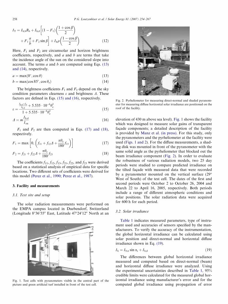
Fig. 2. Pyrheliometer for measuring direct-normal and shaded pyranom-eter for measuring diffuse horizontal solar irradiance are positioned on theroof of the facility.

258 P.G. Loutzenhiser et al. / Solar Energy 81 (2007) 254–267

IT ¼ Ih;bRb þ Ih;d ð1� F 1Þ1þ cos b

2

� ��

þ F 1

abþ F 2 sin b

�þ Ihq

1� cos b2

� �ð12Þ

Here, F1 and F2 are circumsolar and horizon brightnesscoefficients, respectively, and a and b are terms that takethe incidence angle of the sun on the considered slope intoaccount. The terms a and b are computed using Eqs. (13)and (14), respectively.

a ¼ maxð0�; cos hÞ ð13Þb ¼ maxðcos 85�; cos hzÞ ð14Þ

The brightness coefficients F1 and F2 depend on the skycondition parameters clearness e and brightness D. Thesefactors are defined in Eqs. (15) and (16), respectively.

e ¼Ih;dþIn

Ih;dþ 5:535 � 10�6h3

z

1þ 5:535 � 10�6h3z

ð15Þ

D ¼ mIh;d

Ion

ð16Þ

F1 and F2 are then computed in Eqs. (17) and (18),respectively.

F 1 ¼ max 0; f11 þ f12Dþphz

180f13

� �� �ð17Þ

F 2 ¼ f21 þ f22Dþphz

180f23 ð18Þ

The coefficients f11, f12, f13, f21, f22, and f23 were derivedbased on a statistical analysis of empirical data for specificlocations. Two different sets of coefficients were derived forthis model (Perez et al., 1990; Perez et al., 1987).

3. Facility and measurements

3.1. Test site and setup

The solar radiation measurements were performed onthe EMPA campus located in Duebendorf, Switzerland(Longitude 8�36 05500 East, Latitude 47�24 01200 North at an

Fig. 1. Test cells with pyranometers visible in the central part of thepicture and green artificial turf installed in front of the test cell.

elevation of 430 m above sea level). Fig. 1 shows the facilitywhich was designed to measure solar gains of transparentfacade components; a detailed description of the facilityis provided by Manz et al. (in press). For this study, onlythe pyranometers and the pyrheliometer at the facility wereused (Figs. 1 and 2). For the diffuse measurements, a shad-ing disk was mounted in front of the pyranometer with thesame solid angle as the pyrheliometer that blocked out thebeam irradiance component (Fig. 2). In order to evaluatethe robustness of various radiation models, two 25 dayperiods were studied to compare predicted irradiance onthe tilted facade with measured data that were recordedby a pyranometer mounted on the vertical surface (29�West of South) of the test cell. The dates of the first andsecond periods were October 2 to October 26, 2004 andMarch 22 to April 16, 2005, respectively. Both periodsinclude a range of different atmospheric conditions andsolar positions. The solar radiation data were acquiredfor 600 h for each period.

3.2. Solar irradiance

Table 1 indicates measured parameters, type of instru-ment used and accuracies of sensors specified by the man-ufacturers. To verify the accuracy of the instrumentation,the global horizontal irradiance can be calculated usingsolar position and direct-normal and horizontal diffuseirradiance shown in Eq. (19).

Ih ¼ Ib;n sin as þ Ih;d ð19Þ

The differences between global horizontal irradiancemeasured and computed based on direct-normal (beam)and horizontal diffuse irradiance were analyzed. Usingthe experimental uncertainties described in Table 1, 95%credible limits were calculated for the measured global hor-izontal irradiance using manufacturer’s error and for thecomputed global irradiance using propagation of error

y = 0.9665x + 0.6466

R2 = 0.9985

0

100

200

300

400

500

600

700

800

0 200 400 600 800Measured global horizontal irradiance, W/m2

Cal

cula

ted

glob

al h

oriz

onta

l irr

adia

nce,

W/m

2

Fig. 3b. Measured and calculated global horizontal irradiance forPeriod 2.

Table 1Instruments used for measuring solar irradiance

Parameter Unit Type of sensor/measurement Number ofsensors

Accuracy

Solar global irradiance,facade plane (29� W of S)

W/m2 Pyranometer (Kipp & Zonen CM 21) 1 ± 2% of reading

Solar global horizontal irradiance W/m2 Pyranometer (Kipp & Zonen CM 21) 1 ± 2% of readingSolar diffuse horizontal irradiance W/m2 Pyranometer, mounted under the shading disc

of a tracker (Kipp & Zonen CM 11)1 ± 3% of reading

Direct-normal irradiance W/m2 Pyrheliometer, mounted in an automaticsun-following tracker(Kipp & Zonen CH 1)

1 ± 2% of reading

P.G. Loutzenhiser et al. / Solar Energy 81 (2007) 254–267 259

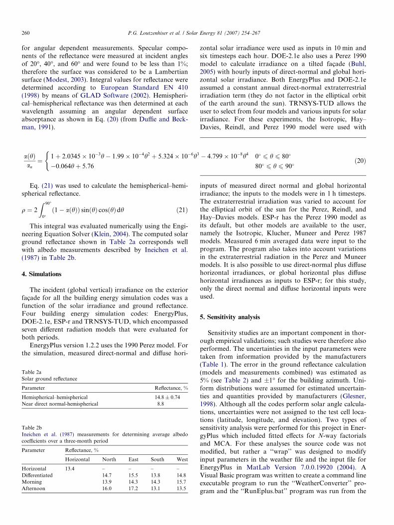
techniques (uncertainty analysis) assuming uniform distri-butions (Glesner, 1998). From these comparisons, the95% credible limits from the calculated and measured glo-bal horizontal irradiance for Periods 1 and 2 were found tooverlap 78.0% and 70.1% of the time, respectively; thesecalculations were only performed when the sun was up(as > 0). Careful examination of these results reveals thatthe discrepancies occurred when the solar altitude anglesand irradiance were small or the solar irradiance were verylarge (especially for Period 2). Linear regression analysiswas used to compare the computed global irradiance usingmeasured beam and diffuse irradiances and measured glo-bal irradiances. The results from this analysis are shownfor Periods 1 and 2 in Figs. 3a and 3b, respectively. The dif-ferences between calculated and measured quantities areapparent from the slopes of lines. These results reveal aslight systematic under-prediction by roughly 3% of globalhorizontal irradiance when calculating it from the beamand diffuse horizontal irradiance components.

14

16

3.3. Ground reflectance

The importance of accurately quantifying the albedo inlieu of relying on default values is discussed in detail byIneichen et al. (1987). Therefore, in order to have a well-defined and uniform ground reflectance, artificial green turf

y = 0.9741x - 0.4356

R2 = 0.9977

0

100

200

300

400

500

600

0 100 200 300 400 500 600Measured global horizontal irradiance, W/m2

Cal

cula

ted

glob

al h

orzi

onta

l irr

adia

nce,

W/m

2

Fig. 3a. Measured and calculated global horizontal irradiance forPeriod 1.

was installed in front of the test cell to represent a typicaloutdoor surface (Fig. 1).

Reflectance of a sample of the artificial turf was mea-sured at almost perpendicular (3�) incident radiation inthe wavelength interval between 250 nm and 2500 nm usingan integrating sphere (Fig. 4) which could not be employed

0

2

4

6

8

10

12

250 750 1250 1750 2250Wavelength, nm

Dir

ect-

hem

isph

eric

al r

efle

ctan

ce, %

Fig. 4. Near direct normal-hemispherical reflectance of the artificial turf.

260 P.G. Loutzenhiser et al. / Solar Energy 81 (2007) 254–267

for angular dependent measurements. Specular compo-nents of the reflectance were measured at incident anglesof 20�, 40�, and 60� and were found to be less than 1%;therefore the surface was considered to be a Lambertiansurface (Modest, 2003). Integral values for reflectance weredetermined according to European Standard EN 410(1998) by means of GLAD Software (2002). Hemispheri-cal–hemispherical reflectance was then determined at eachwavelength assuming an angular dependent surfaceabsorptance as shown in Eq. (20) (from Duffie and Beck-man, 1991).

aðhÞan¼ 1þ 2:0345� 10�3h� 1:99� 10�4h2 þ 5:324� 10�6h3 � 4:799� 10�8h4 0� 6 h 6 80�

�0:064hþ 5:76 80� 6 h 6 90�

(ð20Þ

Eq. (21) was used to calculate the hemispherical–hemi-spherical reflectance.

q ¼ 2

Z 90�

0�ð1� aðhÞÞ sinðhÞ cosðhÞdh ð21Þ

This integral was evaluated numerically using the Engi-neering Equation Solver (Klein, 2004). The computed solarground reflectance shown in Table 2a corresponds wellwith albedo measurements described by Ineichen et al.(1987) in Table 2b.

4. Simulations

The incident (global vertical) irradiance on the exteriorfacade for all the building energy simulation codes was afunction of the solar irradiance and ground reflectance.Four building energy simulation codes: EnergyPlus,DOE-2.1e, ESP-r and TRNSYS-TUD, which encompassedseven different radiation models that were evaluated forboth periods.

EnergyPlus version 1.2.2 uses the 1990 Perez model. Forthe simulation, measured direct-normal and diffuse hori-

Table 2aSolar ground reflectance

Parameter Reflectance, %

Hemispherical–hemispherical 14.8 ± 0.74Near direct normal-hemispherical 8.8

Table 2bIneichen et al. (1987) measurements for determining average albedocoefficients over a three-month period

Parameter Reflectance, %

Horizontal North East South West

Horizontal 13.4 – – – –Differentiated 14.7 15.5 13.8 14.8Morning 13.9 14.3 14.3 15.7Afternoon 16.0 17.2 13.1 13.5

zontal solar irradiance were used as inputs in 10 min andsix timesteps each hour. DOE-2.1e also uses a Perez 1990model to calculate irradiance on a tilted facade (Buhl,2005) with hourly inputs of direct-normal and global hori-zontal solar irradiance. Both EnergyPlus and DOE-2.1eassumed a constant annual direct-normal extraterrestrialirradiation term (they do not factor in the elliptical orbitof the earth around the sun). TRNSYS-TUD allows theuser to select from four models and various inputs for solarirradiance. For these experiments, the Isotropic, Hay–Davies, Reindl, and Perez 1990 model were used with

inputs of measured direct normal and global horizontalirradiance; the inputs to the models were in 1 h timesteps.The extraterrestrial irradiation was varied to account forthe elliptical orbit of the sun for the Perez, Reindl, andHay–Davies models. ESP-r has the Perez 1990 model asits default, but other models are available to the user,namely the Isotropic, Klucher, Muneer and Perez 1987models. Measured 6 min averaged data were input to theprogram. The program also takes into account variationsin the extraterrestrial radiation in the Perez and Muneermodels. It is also possible to use direct-normal plus diffusehorizontal irradiances, or global horizontal plus diffusehorizontal irradiances as inputs to ESP-r; for this study,only the direct normal and diffuse horizontal inputs wereused.

5. Sensitivity analysis

Sensitivity studies are an important component in thor-ough empirical validations; such studies were therefore alsoperformed. The uncertainties in the input parameters weretaken from information provided by the manufacturers(Table 1). The error in the ground reflectance calculation(models and measurements combined) was estimated as5% (see Table 2) and ±1� for the building azimuth. Uni-form distributions were assumed for estimated uncertain-ties and quantities provided by manufacturers (Glesner,1998). Although all the codes perform solar angle calcula-tions, uncertainties were not assigned to the test cell loca-tions (latitude, longitude, and elevation). Two types ofsensitivity analysis were performed for this project in Ener-gyPlus which included fitted effects for N-way factorialsand MCA. For these analyses the source code was notmodified, but rather a ‘‘wrap’’ was designed to modifyinput parameters in the weather file and the input file forEnergyPlus in MatLab Version 7.0.0.19920 (2004). AVisual Basic program was written to create a command lineexecutable program to run the ‘‘WeatherConverter’’ pro-gram and the ‘‘RunEplus.bat’’ program was run from the

MatLabProgram

Weather Processor Inputs• Direct-Normal Irradiance• Diffuse Horizontal

Irradiance

EnergyPlusWeather Converter

EnergyPlus InputFile ParametersGround Reflectance

EnergyPlusProgram

EnergyPlus Output ParametersIncident Irradiance on the Facade

UncertaintyOutput

Fig. 5. Flowchart for the sensitivity studies.

P.G. Loutzenhiser et al. / Solar Energy 81 (2007) 254–267 261

MatLab program. Output from each run was recorded inoutput files. A flowchart for this process is depicted inFig. 5.

5.1. Fitted effects for N-way factorials

A fitted effects N-way factorial method was used to iden-tify the impact of uncertainties in various parameters onthe results (Vardeman and Jobe, 2001). The parametersthat were varied for this study included: ground reflectance,building azimuth, direct-normal irradiance, global horizon-tal irradiance (which was an unused parameter in Energy-Plus), and diffuse irradiance. Therefore, for this study afitted effects for a Three-way factorial analysis was per-formed. The first step in this process is to run a one-wayfactorial shown in Eq. (22) varying each parameter. Thisequation is equivalent to the commonly used differentialsensitivity analysis.

ui ¼ /ðni þ riÞ � /ðniÞ ð22Þ

For uniform distributions, the standard deviation is esti-mated in Eq. (23).

ri ¼dffiffiffi3p ð23Þ

Table 3Average factorial impacts (as > 0)

Factorial Period 1

Forward differencing, W/m2 Backward differencing, W/m

Ibn 1.13 �1.10Ih,d 1.37 �1.28q 0.357 �0.357/b �0.499 0.500Ibn · Ih,d �0.05596 �0.0831Ibn · q 0.00155 0.00158Ibn · /b �0.00464 �0.00464Ih,d · q 0.00352 0.00380Ih,d · /b �0.00267 �0.00264q · /b No interactions No interactionsu 2.40 2.40

The two-way factorials were estimated using Eq. (24).Additional levels of interactions were considered but werefound to be negligible.

uij ¼ /ðni þ ri; nj þ rjÞ � ð/ðni; njÞ þ ui þ ujÞ i 6¼ j ð24Þ

The overall uncertainty was estimated using the quadra-ture summation shown in Eq. (25).

u ¼ffiffiffiffiffiffiffiffiffiffiffiffiffiffiffiffiffiffiffiffiffiffiffiffiffiffiffiffiffiffiffiX

u2i þ

Xu2

ij

qð25Þ

This analysis assumes a localized linear relationshipwhere the function is evaluated. To confirm this assump-tion, estimates were made by forward differencing (ni + ri)and backward differencing (ni � ri). The individual factori-als can also be analyzed to assess their impact. In Table 3,the results from this analysis averaged over the entire test(as > 0) are shown for both forward and backward differ-encing. Looking at the results from forward and backwarddifference, the assumed localized linear relationship seemsreasonable but may lead to minor discrepancies that arediscussed later.

5.2. Monte Carlo analysis

The Monte Carlo method can be used to analyze theimpact of all uncertainties simultaneously by randomlyvarying the main input parameters and performing multi-ple evaluations of the output parameter(s). When settingup the analysis, the inputs are modified according to aprobability density function (pdf) and, after numerous iter-ations, the outputs are assumed to be Gaussian (normal) bythe Central Limit Theorem. The error is estimated by tak-ing the standard deviation of the multiple evaluations ateach time step. MatLab 7.0 can be used to generate ran-dom numbers according to Gaussian, uniform, and manyother distributions. A comprehensive description and theunderlying theory behind the Monte Carlo Method areprovided by Fishman (1996) and Rubinstein (1981).

5.2.1. Sampling

For this study, Latin hypercube sampling was used. Inthis method, the range of each input factor is divided into

Period 2

2 Forward differencing, W/m2 Backward differencing, W/m2

1.23 �1.311.50 �1.590.566 �0.566�0.291 0.303

0.0663 0.05310.00308 0.00310�0.0027 �0.00274

0.00514 0.00516�0.00094 �0.000907No interactions No interactions

2.85 2.95

262 P.G. Loutzenhiser et al. / Solar Energy 81 (2007) 254–267

equal probability intervals based on the number of runs ofthe simulation; one value is then taken from each interval.When applying this method for this study given parameterswith non-uniform distributions, the intervals were definedusing the cumulative distribution function and then onevalue was selected from each interval assuming a uniformdistribution (again this was simplified in using MatLabbecause the functions were part of the code). This methodof sampling is better when a few components of input dom-inate the output (Saltelli et al., 2000). For this study, theinput parameters were all sampled from a uniform distribu-tion. Previous studies have shown that after 60–80 runsthere are only slight gains in accuracy (Furbringer andRoulet, 1995), but 120 runs were used to determine uncer-tainty. The average overall uncertainties (as > 0) for Peri-ods 1 and 2 were 2.35 W/m2 and 2.87 W/m2, respectively;the results corresponded well with the fitted effects model.The results at any given time step are discussed in the nextSection (5.3).

5.2.2. Analysis of output

It can be shown that despite the pdf’s for input param-eters, the output parameters will always have a Gaussiandistribution (given a large enough sample and sufficientnumber of inputs) by the Central Limit Theorem; there-fore a Lilliefore Test for goodness of fit to normal distri-bution was used to test significance at 5% (when as > 0).Using this criterion, 27.5% and 11.5% of the outputs fromPeriods 1 and 2, respectively, were found not to be nor-mally distributed. A careful study of these results revealsthat the majority of these discrepancies occurred whenthe direct-normal irradiance is small or zero. This maybe due to the proportional nature of the uncertainties usedfor these calculations. At low direct-normal irradiances,the calculation becomes a function of only three inputsrather than four, which could make the pdf for the outputparameter more susceptible to the individual pdf’s of theinput parameters, which for these cases were uniformdistributions.

5.3. Estimated uncertainties

Estimates for uncertainties were obtained from both fit-ted effects for N-way factorial and MCA. From these anal-yses, both methods yield similar results. The onlydiscrepancies for both forward and backward differencingwere that fitted effects estimates are sometimes overesti-mated at several individual timesteps. Careful inspectionof the individual responses revealed that there was a signif-icant jump in the two-way direct-normal/diffuse response(sometimes in the order of 5 W/m2) that corresponds toodd behavior in the one-way responses. The response forthe rest of the timesteps was negligible. Additional reviewshowed that these events do not occur during the sametimesteps for forward and backward differencing. It wastherefore assumed that these discrepancies result fromlocalized non-linearities at these timesteps.

6. Results

The computed results from the four simulation codeswere compared with the measured global vertical irradi-ance. Comparisons were made using the nomenclatureand methodology proposed by Manz et al. (in press). Animportant term used for comparing the performance ofthe respective models in the codes is the uncertainty ratio.This term was computed at each hour (as > 0) and is shownin Eq. (26). The average, maximum, and minimum quanti-ties are summarized in the statistical analyses for each test.Ninety-five percent credible limits were calculated from theMCA for EnergyPlus and the 95% credible limits for theexperiment were estimated assuming a uniform distribu-tion. The credible limits from EnergyPlus were used to cal-culate the uncertainty ratios for all the models and codes.For the uncertainty ratio, terms less than unity indicatethat the codes were validated with 95% credible limits.

UR ¼ jDjOUExperiment þOUEnergyPlus

ð26Þ

Tables 4–6 show the results from Periods 1 and 2 andcombined periods, respectively. Plots were constructed thatdepict the global vertical irradiation (hourly averaged irra-diance values multiplied by a 1 h interval) and credible lim-its. For these plots, the output and 95% credible limits for agiven hour of the day were averaged to provide an over-view of the performance of each model. Figs. 6–8 containresults from Periods 1 and 2 and the combined results.

7. Discussion and conclusions

The accuracy of the individual radiation models andtheir implementation in each building energy simulationcode for both periods can be accurately assessed from thestatistical analyses and the plots from the results section.Fig. 6 shows that in the morning, there are both overand under-prediction of the global vertical irradiance bythe models for Period 1; in the afternoon the global verticalirradiance is significantly under-predicted by most models.During Period 2, the majority of the models over-predictthe global vertical irradiance for most hours during theday. Combining these results helps to redistribute thehourly over and under-predictions from each model, butit is still clear when comparing the uncertainty ratios thatall the models performed better during Period 1.

Using the average uncertainty ratio as a guide, it can beseen that for both periods none of the models were withinoverlapping 95% credible limits. Strictly speaking, none ofthe models can therefore be considered to be validatedwithin the defined credible limits ðUR > 1Þ. This is partlydue to the proportional nature of the error which at verti-cal irradiance predictions with small uncertainties leads tolarge hourly uncertainty ratio calculations and the diffi-culty in deriving a generic radiation model for every loca-tion in the world. This is also shown in Figs. 6–8 where

Table 4Analysis of global vertical facade irradiance in W/m2 (as > 0) for Period 1

Experiment EnergyPlusPerez 1990

DOE-2.1ePerez 1990

TRNSYS-TUDHay–Davies

TRNSYS-TUDIsotropic

TRNSYS-TUD Reindl

TRNSYS-TUD Perez1990

ESP-rPerez 1990

ESP-rPerez 1987

ESP-rKlucher

ESP-rIsotropic

ESP-rMuneer

�x 176.1 169.7 177.2 165.1 157.8 170.9 169.8 188.2 192.8 174.8 171.9 191.4s 223.8 211.8 218.6 205.1 190.1 209.4 211.1 218.2 220.5 196.9 192.5 226.3xmax 856.8 817.8 820.4 801.2 743.2 810.4 796.4 804.7 806.7 743.5 728.8 915.7xmin 0.2 0.3 0.0 0.4 0.9 0.4 0.3 0.2 0.1 0.3 0.3 0.2D – �6.4 1.1 �11.0 �18.3 �5.2 �6.3 1.9 6.6 �11.5 �14.3 5.1jDj – 13.7 10.5 18.0 26.2 15.7 11.7 13.3 14.7 24.6 27.8 14.1Dmax – 103.5 67.1 108.0 138.9 90.4 73.3 87.7 86.7 139.1 157.7 205.5Dmin – 0.0 0.0 0.0 0.0 0.0 0.0 0.0 0.0 0.0 0.0 0.0Drms – 24.2 17.0 28.9 44.4 24.0 21.0 21.4 22.1 39.1 44.7 24.6D95% – 56.4 40.3 71.7 111.2 56.3 57.1 50.9 51.5 96.5 110.7 53.3OU 6.90 4.62 – – – – – – – – – –UR – 1.34 1.34 2.28 4.03 2.29 1.12 1.43 1.69 2.50 2.63 1.54URmax – 12.42 20.41 20.41 129.05 20.41 10.20 11.22 12.09 17.04 17.04 13.48URmin – 0.00 0.01 0.00 0.00 0.00 0.00 0.00 0.00 0.01 0.00 0.00jDj=�x – 7.8 5.9 10.2 14.9 8.9 6.7 6.7 6.7 14.8 16.7 7.2D=�x – �3.7 0.6 �6.2 �10.4 �3.0 �3.6 �2.7 �0.1 �11.3 �13.4 1.0

Table 5Analysis of global vertical facade irradiance in W/m2 (as > 0) for Period 2

Experiment EnergyPlusPerez 1990

DOE-2.1ePerez 1990

TRNSYS-TUDHay–Davies

TRNSYS-TUDIsotropic

TRNSYS-TUDReindl

TRNSYS-TUD Perez1990

ESP-rPerez1990

ESP-rPerez1987

ESP-rKlucher

ESP-rIsotropic

ESP-rMuneer

�x 194.5 208.5 210.5 199.7 191.6 207.7 201.4 202.0 206.7 190.1 187.9 202.5s 222.1 226.3 231.3 219.0 201.5 224.1 225.2 222.4 223.8 201.3 197.3 224.2xmax 797.1 796.3 828.5 807.8 741.4 820.2 801.7 794.6 799.5 730.4 720.2 801.1xmin 0.3 0.3 0.0 0.4 0.4 0.4 0.3 0.2 0.2 0.3 0.3 0.2D – 14.0 16.0 5.2 �2.9 13.2 6.9 7.5 12.2 �4.4 �6.6 8.0jDj – 19.4 17.6 16.2 25.0 19.0 12.7 14.6 17.2 23.4 26.4 15.4Dmax – 104.0 77.3 59.5 122.6 67.2 63.5 81.3 86.7 113.0 134.9 86.9Dmin – 0.0 0.1 0.1 0.1 0.1 0.0 0.0 0.0 0.0 0.0 0.0Drms – 29.2 26.3 20.9 35.2 24.5 19.2 22.2 24.5 33.6 38.8 24.0D95% – 70.1 62.4 42.6 81.7 51.1 46.3 50.9 58.0 79.9 93.2 55.6OU 7.62 5.62 – – – – – – – – – –UR – 2.11 2.12 2.66 3.06 2.99 1.41 1.61 2.00 2.60 2.73 1.64URmax – 12.83 21.70 20.62 20.63 21.41 11.21 9.70 11.24 14.94 14.94 13.48URmin – 0.00 0.02 0.01 0.03 0.01 0.01 0.00 0.00 0.01 0.01 0.00jDj=�x – 10.0 9.1 8.3 12.9 9.8 6.5 7.5 8.8 12.0 13.6 7.9D=�x – 7.2 8.2 2.7 �1.5 6.8 3.5 3.9 6.3 �2.3 �3.4 4.1

P.G

.L

ou

tzenh

iseret

al.

/S

ola

rE

nerg

y8

1(

20

07

)2

54

–2

67

263

ble

6n

alys

iso

fgl

ob

alve

rtic

alfa

cad

eir

rad

ian

cein

W/m

2(a

s>

0)fo

rb

oth

per

iod

s

Exp

erim

ent

En

ergy

Plu

sP

erez

1990

DO

E-2

.1e

Per

ez19

90T

RN

SY

S-T

UD

Hay

–Dav

ies

TR

NS

YS

-T

UD

Iso

tro

pic

TR

NS

YS

-T

UD

Rei

nd

l

TR

NS

YS

-T

UD

Per

ez19

90

ES

P-r

Per

ez19

90

ES

P-r

Per

ez19

87

ES

P-r

Klu

cher

ES

P-r

Iso

tro

pic

ES

P-r

Mu

nee

r

186.

219

1.0

195.

518

4.1

176.

319

1.1

187.

118

8.2

192.

817

4.8

171.

919

1.4

222.

922

0.6

226.

121

3.4

197.

021

8.2

219.

421

8.2

220.

519

6.9

192.

522

6.3

ax

856.

881

7.8

828.

580

7.8

743.

282

0.2

801.

780

4.7

806.

774

3.5

728.

891

5.7

in0.

20.

30.

00.

40.

40.

40.

30.

20.

10.

30.

30.

2–

4.8

9.3

�2.

1�

9.9

4.9

0.9

1.9

6.6

�11

.5�

14.3

5.1

j–

16.8

14.4

17.0

25.6

17.5

12.2

13.3

14.7

24.6

27.8

14.1

max

–10

4.0

77.3

108.

013

8.9

90.4

73.3

87.7

86.7

139.

115

7.7

205.

5

min

–0.

00.

00.

00.

00.

00.

00.

00.

00.

00.

00.

0

rms

–27

.122

.624

.839

.624

.320

.021

.422

.139

.144

.724

.6

95%

–65

.755

.154

.999

.454

.248

.750

.951

.596

.511

0.7

53.3

U7.

304.

46–

––

––

––

––

–R

–1.

911.

902.

573.

612.

771.

381.

431.

692.

502.

631.

54R

max

–17

.62

29.3

128

.31

129.

0529

.39

15.3

811

.22

12.0

917

.04

17.0

413

.48

Rm

in–

0.00

0.01

0.00

0.00

0.00

0.00

0.00

0.00

0.01

0.00

0.00

j=� x

–9.

07.

79.

113

.79.

46.

67.

27.

913

.214

.97.

6=�

x–

2.6

5.0

�1.

1�

5.3

2.6

0.5

1.0

3.5

�6.

2�

7.7

2.8

264 P.G. Loutzenhiser et al. / Solar Energy 81 (2007) 254–267

Ta

A �x s xm

xm D jD D D D D O U U U jD D

there is very little overlap in the experimental and MCA95% credible limits. But the average uncertainty ratio canalso be used as a guide to rank the overall performanceof the tilted radiation models. The Isotropic model per-formed the worst during these experiments, which can beexpected because it was the most simplistic and did notaccount for the various individual components of diffuseirradiance. While the Reindl and Hay–Davies modelaccounted for the additional components of diffuse irradi-ance (both circumsolar and horizontal brightening for theReindl and circumsolar for the Hay–Davies), the Perez for-mulation – which relied on empirical data to quantify thediffuse components – provided the best results for this loca-tion and wall orientation. Differences between the Perezmodels in the four building energy simulation codes canbe attributed to solar irradiance input parameters (beam,global horizontal, and diffuse), timesteps of the weathermeasurements, solar angle algorithms, and assumptionsmade by the programmers (constant direct-normal extra-terrestrial radiations for DOE-2.1e and EnergyPlus). Forboth periods, the assumptions made in the TRNSYS-TUD formulation Perez radiation model performed best.But also from these results, the Muneer model performedquite well without the detail used in the Perez models. Infact, the Muneer model performed better than Perez mod-els formulated in EnergyPlus and DOE-2.1e.

The presented results reveal distinct differences betweenradiation models that will ultimately manifest themselves inthe solar gain calculations. Mean absolute deviations inpredicting solar irradiance for both time periods were: (1)13.7% and 14.9% for the isotropic sky model, (2) 9.1%for the Hay–Davies, (3) 9.4 % for the Reindl, (4) 7.6%for the Muneer model, (5) 13.2% for the Klucher, (6)9.0%, 7.7%, 6.6%, and 7.1% for the 1990 Perez, and (7)7.9% for the 1987 Perez models. This parameter is a goodestimate of the instantaneous error that would impact peakload calculations. The mean deviations calculations forthese time periods were: (1) �5.3% and �7.7% for the iso-tropic sky model, (2) �1.1% for the Hay–Davies, (3) 2.6%for the Reindl, (4) 2.8% for the Muneer model, (5) �6.2%for the Klucher, (6) 2.6%, 5.0%, 0.5%, and 1.0% for the1990 Perez, and (7) 3.5% for the 1987 Perez models. Fromthis parameter it can be concluded that building energysimulation codes with advanced radiation models are capa-ble of computing total irradiated solar energy on buildingfacades with a high precision for longer time periods (suchas months). Hence, the calculations of building energy con-sumption with high prediction accuracy is achievable evenin today’s highly glazed buildings, which are largelyaffected by solar gains. On the other hand, even the mostadvanced models deviate significantly at specific hourlytimesteps (up to roughly 100 W/m2), which poses seriouslimitations to accuracy of predictions of cooling power ata specific point in time, the short-time temperature fluctu-ations in the case of non-air conditioned buildings or thecontrol and/or sizing of HVAC equipment or shadingdevices. When performing building simulations, engineers

Fig. 6. Average hourly irradiation comparisons for the vertical facade for Period 1.

Fig. 7. Average hourly irradiation comparisons for the vertical facade for Period 2.

Fig. 8. Average hourly irradiation comparisons for the vertical facade combining both periods.

P.G. Loutzenhiser et al. / Solar Energy 81 (2007) 254–267 265

266 P.G. Loutzenhiser et al. / Solar Energy 81 (2007) 254–267

must consider much higher uncertainties at specifictimesteps.

Additional factors that were not investigated include thenumber of components of solar irradiance measured at agiven weather station (often only global horizontal irradi-ance is measured and other models are used to computebeam irradiance), locations and densities of the weatherstations used as inputs for building simulation codes, andreliability of weather files used by building energy simula-tion codes. While this study is somewhat limited to a spe-cific location and time period, it reveals the importanceof making proper assessments concerning tilted radiationmodels and their implementations in building energy simu-lation codes.

Note: Radiation data and data of all other experimentswithin the IEA Task 34 project can be downloaded fromour website at www.empa.ch/ieatask34.

Acknowledgements

We gratefully acknowledge with thanks the financialsupport from the Swiss Federal Office of Energy (BFE)for building and testing the experimental facility (Project17 0166) as well as the funding for EMPA participation inIEA Task 34/43 (Project 100 0765). We would also like toacknowledge Dr. M. Morris from the Iowa State Univer-sity Statistics Department for his clear direction with re-gard to formulating the sensitivity analysis and the manycontributions from our colleagues R. Blessing, S. Carl,M. Camenzind, and R. Vonbank.

References

Aude, P., Tabary, L., Depecker, P., 2000. Sensitivity analysis andvalidation of buildings’ thermal models using adjoint-code method.Energy and Buildings 30, 267–283.

Badescu, V., 2002. 3D isotropic approximation for solar diffuse irradianceon tilted surfaces. Renewable Energy 26, 221–233.

Behr, H.D., 1997. Solar radiation on tilted south oriented surfaces:validation of transfer-models. Solar Energy 61 (6), 399–413.

Buhl, F., 2005. Private email correspondence exchanged on March 9, 2005with Peter Loutzenhiser at EMPA that contained the radiation modelportion of the DOE-2.1E source code, Lawrence Berkley NationalLaboratories (LBNL).

DOE-2.1E, (Version-119). 2002. Building Energy Simulation Code,(LBNL), Berkley, CA, April 9, 2002.

Duffie, J.A., Beckman, W.A., 1991. Solar Engineering of ThermalProcesses, Second ed. John Wiley & Sons, New York, Chichester,Brisbane, Toronto, Singapore.

EnergyPlus Version, 1.2.2.030. 2005. Building Energy simulation code.Available from: <www.energyplus.gov>.

ESP-r, Version 10.12, 2005. University of Strathclyde. Available from:<www.esru.strath.ac.uk>.

European Standard EN 410, 1998. Glass in building – determination ofluminous and solar characteristics of glazing. European Committee forStandardization, Brussels, Belgium.

Fishman, G.S., 1996. Monte Carlo: Concepts, Algorithms, and Applica-tions. Springer, New York Berlin Heidelberg.

Furbringer, J.M., Roulet, C.A., 1995. Comparison and combination offactorial and Monte-Carlo design in sensitivity analysis. Building andEnvironment 30 (4), 505–519.

Furbringer, J.M., Roulet, C.A., 1999. Confidence of simulation results:put a sensitivity analysis module in you MODEL: the IEA-ECBCSAnnex 23 experience of model evaluation. Energy and Buildings 30,61–71.

GLAD Software, 2002. Swiss Federal Laboratories for Materials Testingand Research (EMPA), Duebendorf, Switzerland.

Glesner, J.L., 1998. Assessing uncertainty in measurement. StatisticalScience 13 (3), 277–290.

Gueymard, C., 1987. An anisotropic solar irradiance model for tiltedsurfaces and its comparison with selected engineering algorithms. SolarEnergy 38 (5), 367–386.

Hay, J.E., Davies, J.A., 1980. Calculations of the solar radiation incidenton an inclined surface. In: Hay, J.E., Won, T.K. (Eds.), Proc. of FirstCanadian Solar Radiation Data Workshop, 59. Ministry of Supplyand Services, Canada.

Hottel, H.C., Woertz, B.B., 1942. Evaluation of flat-plate solar heatcollector. Trans. ASME 64, 91.

Ineichen, P., Perez, R., Seals, R., 1987. The importance of correct albetodetermination for adequately modeling energy received by a tiltedsurface. Solar Energy 39 (4), 301–305.

Klein, S.A., 2004. Engineering Equation Solver (EES) Software, Depart-ment of Mechanical Engineering. University of Wisconsin, Madison.

Klucher, T.M., 1979. Evaluation of models to predict insolation on tiltedsurfaces. Solar Energy 23 (2), 111–114.

Li, D.H.W., Lam, J.C., Lau, C.C.S., 2002. A new approach forpredicting vertical global solar irradiance. Renewable Energy 25,591–606.

Liu, B.Y.H., Jordan, R.C., 1960. The interrelationship and characteristicdistribution of direct, diffuse, and total solar radiation. Solar Energy 4(3), 1–19.

Lomas, K.J., Eppel, H., 1992. Sensitivity analysis techniques for buildingthermal simulation programs. Energy and Buildings 19, 21–44.

Macdonald, I., Strachan, P., 2001. Practical applications of uncertaintyanalysis. Energy and Buildings 33, 219–227.

Manz, H., Loutzenhiser, P., Frank, T., Strachan, P.A., Bundi, R., andMaxwell, G., in press. Series of experiments for empirical validation ofsolar gain modeling in building energy simulation codes – Experimen-tal setup, test cell characterization, specifications and uncertaintyanalysis. Building and Environment.

Mara, T.A., Garde, F., Boyer, H., Mamode, M., 2001. Empiricalvalidation of the thermal model of a passive solar test cell. Energyand Buildings 33, 589–599.

MatLab Version 7.0.0.19920, 2004. The MathWorks Inc.Modest, M., 2003. Radiative Heat Transfer, Second ed. Academic Press,

Amsterdam.Muneer, T., 1997. Solar Radiation and Daylight Models for the Energy

Efficient Design of Buildings. Architectural Press, Oxford.Olmo, F.J., Vida, J., Castro-Diez, Y., Alados-Arboledas, L., 1999.

Prediction of global irradiance on inclined surfaces from horizontalglobal irradiance. Energy 24, 689–704.

Palomo del Barrio, E., Guyon, G., 2003. Theoretical basis for empiricalmodel validation using parameter space analysis tools. Energy andBuildings 35, 985–996.

Palomo del Barrio, E., Guyon, G., 2004. Application of parameters spaceanalysis tools fro empirical model validation. Energy and Buildings 36,23–33.

Perez, R., Stewart, R., Arbogast, C., Seals, R., Scott, J., 1986. Ananisotropic hourly diffuse radiation model for sloping surfaces:Description, performanace validation, site dependency evaluation.Solar Energy 36 (6), 481–497.

Perez, R., Seals, R., Ineichen, P., Stewart, R., Menicucci, D., 1987. A newsimplified version of the Perez diffuse irradiance model for tiltedsurfaces. Solar Energy 39 (3), 221–232.

Perez, R., Ineichen, P., Seals, R., Michalsky, J., Stewart, R., 1990.Modeling daylight availability and irradiance components from directand global irradiance. Solar Energy 44 (5), 271–289.

Reindl, D.T., Beckmann, W.A., Duffie, J.A., 1990a. Diffuse fractioncorrelations. Solar Energy 45 (1), 1–7.

P.G. Loutzenhiser et al. / Solar Energy 81 (2007) 254–267 267

Reindl, D.T., Beckmann, W.A., Duffie, J.A., 1990b. Evaluation of hourlytilted surface radiation models. Solar Energy 45 (1), 9–17.

Remund, J., Salvisberg, E., Kunz, S., 1998. On the generation of hourlyshortwave radiation data on tilted surfaces. Solar Energy 62 (5),331–334.

Robledo, L., Soler, A., 2002. A simple clear skies model for the luminousefficacy of diffuse solar radiation on inclined surfaces. RenewableEnergy 26, 169–176.

Rubinstein, R.Y., 1981. Simulation and the Monte Carlo Method. JohnWiley & Sons, New York, Chichester, Brisbane, Toronto.

Saltelli, A., Chan, K., Scott, E.M., 2000. Sensitivity Analysis. John Wiley& Sons, Ltd, Chichester, New York, Weinheim, Brisbane, Singapore,Toronto.

Saltelli, A., Tarantola, S., Campolongo, F., Ratto, M., 2004. SensitivityAnalysis in Practice: A Guide to Assessing Scientific Models. JohnWiley & Sons, LTD.

Santner, T.J., Williams, B.J., Notz, W.I., 2003. The Design andAnalysis of Computer Experiments. Springer, New York, Berlin,Heidelberg.

TRNSYS-TUD, 2005. Technical University of Dresden research codebased on the frame of TRNSYS 14.2, Solar Energy Laboratory,University of Wisconsin-Madison, Madison, WI, 1996.

Vardeman, S.B., Jobe, J.M., 2001. Data Collection and Analysis. DuxburyThomson Learning, Australia, Canada, Mexico, Singapore, Spain,United Kingdom, United States.