1

The Heckscher-Ohlin-Samuelson (H-O-S) Model of International Trade1

Some Context

To understand the force of the HO model, one should recognize it in its time. In the 1930s World War I had decimated the major powers on a scale unimaginable to earlier generations, the world was in depression, and economists generally had the Ricardian model to explain comparative advantage albeit with more general approaches to trade that worked on a very broad canvas without systematically linking it to the rewards of specific groups.

The HO approach and Samuelson’s subsequent elaboration of the model brought a strikingly powerful focus to the aftermath of World War II. Not only did he indicate the power of the model to predict factor price behaviour, but he linked the pursuit of free trade with the equalization of factor rewards among countries. This work fit the temper of the times as it encouraged the missions of the newly established institutions -- the World Bank, the GATT and to a lesser degree the IMF– in their missions to reduce tariffs for economic development and the betterment of all. The H-O-S model was the workhorse of international economics during the 1940s through the 1970s and is still used as a benchmark today.

The model

In the same way that different technologies embodied in the input-output coefficients, the aij’s, provided the basis for comparative advantage and trade in the Ricardian model, in the context of the HOS model, countries share a common technology, but differ in their factor endowments: their labour-capital ratios.

The implications of this framework are powerful. It provides an unambiguous answer to who are the winners and losers when relative prices change, but it also makes the case that trade can substitute for factor mobility as factor prices are equalized across countries simply through the agency of trade. Increases in the stock of a factor of production will simultaneously expand output in one of the industries and contract output in the other even though both factors are used in both industries. The model also predicts the pattern of trade based on the relative factor endowments of the participant countries. The country relatively well endowed (compared with the other country) with labour (for example) will export the good that uses that factor intensively. Compared to its trading partner, the good having a relatively low price in autarky will be exported, and production will tend to specialize in the good that is exported.

The fact that the countries share a common technology is a strong assumption, but if everyone can read the same set of plans and consequently have access to the same technology, then differences in production and the pattern of trade must come from elsewhere.

Such a logical and interesting framework has been subjected to extensive empirical testing. The paradoxical nature of the results of this testing have generated tremendous interest in the elaborations and extension of the model.

1 Although developed by Bertil Ohlin, a student of Eli Heckscher in the early 1930s, a formal statement and development of results and extensions by Paul Samuelson were sufficiently substantial that he is often ‘awarded a hyphen’ when discussing the model.

2

The Assumptions of H-O-S

1. Two countries can both produce the same two goods, x1, and x2. Both countries use the same technology to produce the same good. Both goods production display constant returns to scale in each industry and both capital and labour are used in both industries.

2. Both countries use capital and labour that are perfectly mobile within the country, but immobile across countries. We will assume full employment so that the amounts of labour and capital fulfill the constraints:

3. a. L=aL1x1+aL2x2 b. K=aK1x1+aK2x2

The labour constraint is of course the same as the labour constraint in Ricardo, and the capital constraint is analogous and is discussed below.

4. The difference between the two industries within each country is characterized by different relative factor intensities; the difference in the capital-labour ratios used in production. We will assume that industry 1 is relatively labour intensive (and industry 2 is relatively capital intensive) so that :

5. a. 𝐾𝐾1

𝐿𝐿1< 𝐾𝐾2

𝐿𝐿2 → 𝑎𝑎𝐾𝐾1

𝑎𝑎𝐿𝐿1< 𝑎𝑎𝐾𝐾2

𝑎𝑎𝐿𝐿2 The second expression is the same as the first. Divide both the

numerator and the denominator by their respective outputs. b. 𝐿𝐿2

𝐾𝐾2< 𝐿𝐿1

𝐾𝐾1 → 𝑎𝑎𝐿𝐿2

𝑎𝑎𝐾𝐾2< 𝑎𝑎𝐿𝐿1

𝑎𝑎𝐾𝐾1 is the same as (a) and simply emphasizes that industry 1 is labour

intensive symbolically.

The notion of factor intensities is a key ingredient of the HOS model.

6. Factor and goods markets are competitive. 7. Countries differ in their relative endowments of capital and labour. In the two-country case we

assume (arbitrarily) that the home country is relatively labour abundant2:

a. �𝐾𝐾𝐿𝐿�𝐹𝐹

> �𝐾𝐾𝐿𝐿�𝐻𝐻

8. We assume that consumers have the same tastes in both countries and their relative demands

are unaffected by income. (This is a convenience, but it is useful insofar as it allows us to highlight the role played by the different endowments in giving rise to trade.)

9. There are some additional assumptions associated with the model, but they are overly nuanced for a first pass. We will refer to them if needed: factor intensity reversals, sufficiently similar endowments of labour and capital between countries, more goods, more factors, less than perfect competition in either the goods or factor markets, and so forth.

Note: Figures follow the Appendices

2 Notice that a country is factor abundant while an industry is factor intensive.

3

Drawing output when coefficients are fixed

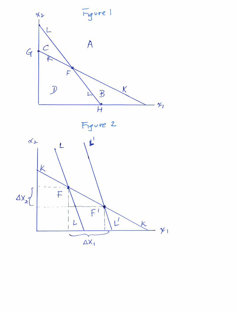
We begin our discussion of the HOS model in the same way we looked at the Ricardian model. Let’s look at the outputs. Recall that when we put x1 and x2 on the axes, we can plot the labour constraint from line (2a) above: LL in Figure 1. However, in Ricardo we assumed that the aij’s were fixed. To make our plotting simple, let us assume for the moment that the ais’s are also fixed in HOS. (They are not, but we will get to that in the fullness of time.)

Insert Figure 1 and Figure 2

Further, we only had a single factor in the Ricardian model. If we are going to add capital, then we need to plot its constraint line, KK. How to put it in? Is it flatter or steeper than the labour constraint line?

Notice that the slope of the labour constraint line is �𝒂𝒂𝑳𝑳𝑳𝑳𝒂𝒂𝑳𝑳𝑳𝑳�. Analogously we can be sure that the capital

constraint line’s slope is �𝒂𝒂𝑲𝑲𝑳𝑳𝒂𝒂𝑲𝑲𝑳𝑳

�. Now, looking at our assumption that industry 1 is labour intensive (3a),

we can be sure that the slope of the labour constraint is steeper. (Can you show why?)

What can we say about what output is possible in Figure 1 -- and recall that output requires both factors of production even though we have fixed the input-output coefficients? First, notice that the two lines cross. That will be a special point as we will see shortly. Second, however, ask in which regions is it possible that production can take place? Clearly, in region A, there can be no production as it lies beyond the amounts of capital and labour in the economy. How about in region B? There is enough capital, but there is not enough labour to use all the capital. If production were to take place, it must lie along the labour constraint line LL, and simultaneously there would be an excess supply of capital.

Analogously, in region C, there is unemployment of labour, and output lies along the capital constraint line KK. In interior region, D, there is unemployment of both labour and capital.

Clearly, the only point of full employment in the figure is point F. It is the only point in which there is no excess supply of either factor and the endowments are fully utilized. The production possibilities frontier is inner hull of the figure FGH and there is unemployment of some factor everywhere but at F.

A first result: Suppose there is an increase in the stock of labour

If the labour stock were to increase – recall that coefficients are fixed – then the slope of the labour constraint line will not change. But because there is more labour, then there must be a parallel shift of the labour constraint line LL to the right as displayed in Figure 2 as L’L’. The full employment point moves from F to F’.3

This is very interesting. Notice that output of industry 1 increases but that output of industry 2 declines! Think about this for a moment. We have increased the endowment of labour and output of one of the industries that uses both labour and capital decreases. Further, think about what this means for output. If labour increases by 10%, for example, then what will happen to output in industry 1, the labour-intensive industry? Looking just at the geometry of the diagram, since the distance between the two parallel capital constraint lines is 10% (by assumption), notice that the horizontal distance between F

3 We keep focussing on the full employment points. It will become clearer why we have this obsession as the model is elaborated in section TBA.

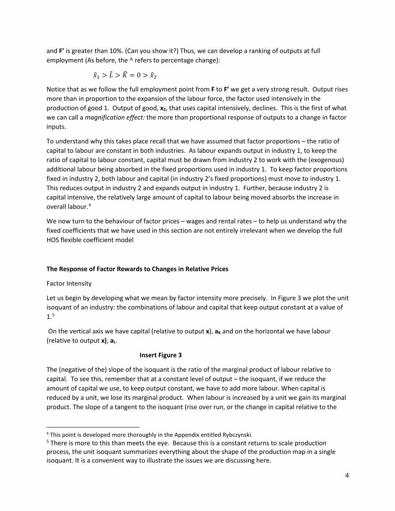
4

and F’ is greater than 10%. (Can you show it?) Thus, we can develop a ranking of outputs at full employment (As before, the ^ refers to percentage change):

𝑥𝑥�1 > 𝐿𝐿� > 𝐾𝐾� = 0 > 𝑥𝑥�2

Notice that as we follow the full employment point from F to F’ we get a very strong result. Output rises more than in proportion to the expansion of the labour force, the factor used intensively in the production of good 1. Output of good, x2, that uses capital intensively, declines. This is the first of what we can call a magnification effect: the more than proportional response of outputs to a change in factor inputs.

To understand why this takes place recall that we have assumed that factor proportions – the ratio of capital to labour are constant in both industries. As labour expands output in industry 1, to keep the ratio of capital to labour constant, capital must be drawn from industry 2 to work with the (exogenous) additional labour being absorbed in the fixed proportions used in industry 1. To keep factor proportions fixed in industry 2, both labour and capital (in industry 2’s fixed proportions) must move to industry 1. This reduces output in industry 2 and expands output in industry 1. Further, because industry 2 is capital intensive, the relatively large amount of capital to labour being moved absorbs the increase in overall labour.4

We now turn to the behaviour of factor prices – wages and rental rates – to help us understand why the fixed coefficients that we have used in this section are not entirely irrelevant when we develop the full HOS flexible coefficient model

The Response of Factor Rewards to Changes in Relative Prices

Factor Intensity

Let us begin by developing what we mean by factor intensity more precisely. In Figure 3 we plot the unit isoquant of an industry: the combinations of labour and capital that keep output constant at a value of 1.5

On the vertical axis we have capital (relative to output x), aK and on the horizontal we have labour (relative to output x), aL.

Insert Figure 3

The (negative of the) slope of the isoquant is the ratio of the marginal product of labour relative to capital. To see this, remember that at a constant level of output – the isoquant, if we reduce the amount of capital we use, to keep output constant, we have to add more labour. When capital is reduced by a unit, we lose its marginal product. When labour is increased by a unit we gain its marginal product. The slope of a tangent to the isoquant (rise over run, or the change in capital relative to the

4 This point is developed more thoroughly in the Appendix entitled Rybczynski. 5 There is more to this than meets the eye. Because this is a constant returns to scale production process, the unit isoquant summarizes everything about the shape of the production map in a single isoquant. It is a convenient way to illustrate the issues we are discussing here.

5

change in labour: ∆𝒂𝒂𝑲𝑲∆𝒂𝒂𝑳𝑳

) is equal to the ratio of the marginal products which in a competitive economy is

equal to the wage-rental ratio, w/r.6 The ray from the origin identifies the factor proportions: the relative quantity of capital to labour used in production.

Cost minimization assures us that the wage-rental ratio (line 1) is tangent to the isoquant at point A.7 Notice that this defines the capital to labour ratio in the industry, �𝒂𝒂𝑲𝑲 𝒂𝒂𝑳𝑳� �. Now let the wage-rental ratio fall to line 2. The tangency moves to point B which displays a lower capital-labour ratio. This makes good sense as with cheaper labour, more labour is used.

This is a good point to remind ourselves how different this model is from Ricardo in terms of what it is we call technology. In Ricardo we saw that the aij’s were fixed, and we kept that assumption in the earlier section so we could draw the picture of output and endowments easily. However, from Figure 3 it is clear that the aij’s need not be constant. Clearly, they change as we move along the isoquant. More precisely, they are themselves functions of the wage-rental ratio. That is: 𝒂𝒂𝒊𝒊𝒊𝒊(

𝒘𝒘𝒓𝒓

).8

In Figure 4 we draw a relationship between outputs in both industries and the wage-rental ratio. The two isoquants represent unit output in each industry. They share a common wage-rental ratio. (Why?) The ray from the origin through point A gives the capital-labour ratio in industry 2: clearly the capital- intensive industry since it uses more capital relative to labour at the common relative prices. The ray from the origin through B gives the capital-labour ratio in industry 1: the labour-intensive industry. The rays give the factor proportions in which labour and capital are used. The amounts of capital and labour used in producing a unit of each industry can be found along the axes.

Insert Figure 4

6 With a constant level of output, an decrease in capital, ∆𝒂𝒂𝑲𝑲 must be compensated by an increase in labour, ∆𝑎𝑎𝐿𝐿, since each increment is paid its marginal product, ∆𝑿𝑿 = 𝟎𝟎 = 𝑴𝑴𝑴𝑴𝑴𝑴𝑲𝑲∆𝒂𝒂𝑲𝑲. +𝑴𝑴𝑴𝑴𝑴𝑴𝑳𝑳∆𝒂𝒂𝑳𝑳 so that: −�∆𝒂𝒂𝑲𝑲

∆𝒂𝒂𝑳𝑳� = 𝑴𝑴𝑴𝑴𝑴𝑴𝑳𝑳

𝑴𝑴𝑴𝑴𝑴𝑴𝑲𝑲.

7 Recall that the firm takes factor prices, w and r, as exogenous, so that a firm’s minimizing of costs requires a choice of L and K, or 𝒂𝒂𝑳𝑳𝒊𝒊 and 𝒂𝒂𝑲𝑲𝒊𝒊 for each industry j. Since the change of the cost function is

zero at the minimum with the choice of K and L, 𝟎𝟎 = 𝒅𝒅𝒅𝒅 = 𝒘𝒘𝒅𝒅𝑳𝑳 + 𝒓𝒓𝒅𝒅𝑲𝑲 → −𝒅𝒅𝑲𝑲𝒅𝒅𝑳𝑳

= 𝒘𝒘𝒓𝒓

. Translated into

our unit price notation: −𝒅𝒅𝒂𝒂𝑲𝑲𝒊𝒊𝒅𝒅𝒂𝒂𝑳𝑳𝒊𝒊

= 𝒘𝒘𝒓𝒓

. 8 In fact, as a preview of coming attractions we can characterize the isoquant’s shape as a function of the relationship between the capital to labour ratio and the wage to rental rate ratio. This is what is meant by the elasticity of substitution between labour and capital. It reflects percentage changes in the capital-labour ratio with respect to a percentage change in the wage-rental ratio:

𝜎𝜎1 = 𝑎𝑎�𝐾𝐾1−𝑎𝑎�𝐿𝐿1𝑤𝑤�−�̂�𝑟

In industry 2 we have a similar relationship:

𝜎𝜎2 = 𝑎𝑎�𝐾𝐾2−𝑎𝑎�𝐿𝐿2𝑤𝑤�−�̂�𝑟

.

6

Thus, by knowing the technology embedded in the isoquants and the wage-rental ratio in the economy we can specify how much labour and capital are used by a unit of output in each industry. This will become important as we explore the general model.

We turn now to something we have looked at before in the context of the Specific Factors model.

Price changes: old friends

As we know from the specific factors model, the relationship between prices and factor rewards in a competitive environment depends upon the factors used in the production of each good. Unlike the specific factors model, in HOS both labour and capital are used in both industries. What differs is in the proportions in which they are used. We write prices in the usual way:

1. 𝑝𝑝1 = 𝑎𝑎𝐿𝐿1𝑤𝑤 + 𝑎𝑎𝐾𝐾1𝑟𝑟

𝑝𝑝2 = 𝑎𝑎𝐿𝐿2𝑤𝑤 + 𝑎𝑎𝐾𝐾2𝑟𝑟

Notice that both prices are functions of the same two variables, labour and capital. How they differ is in how much labour and capital they use.

As in the case of the specific factors model, the key in our discussion is to see how price change is related to factor prices. To this end we look at a small change in the price of good 1, dp1:

2. 𝑑𝑑𝑝𝑝1 = 𝑎𝑎𝐿𝐿1𝑑𝑑𝑤𝑤 + 𝑤𝑤𝑑𝑑𝑎𝑎𝐿𝐿1 + 𝑎𝑎𝐾𝐾1𝑑𝑑𝑟𝑟 + 𝑟𝑟𝑑𝑑𝑎𝑎𝐾𝐾1

Since we know that cost minimization by firms implies the tangency between the cost of production and the unit isoquant (see footnote 2) we are left with an expression for price changes as:

2.1 𝑑𝑑𝑝𝑝1 = 𝑎𝑎𝐿𝐿1𝑑𝑑𝑤𝑤 + 𝑎𝑎𝐾𝐾1𝑑𝑑𝑟𝑟

As before we express the price changes in percentage change form9:

2.2 𝑑𝑑𝑑𝑑1𝑑𝑑1

≡ �̂�𝑝1 = �𝑎𝑎𝐿𝐿1𝑤𝑤𝑑𝑑1

� 𝑑𝑑𝑤𝑤𝑤𝑤

+ �𝑎𝑎𝐾𝐾1𝑟𝑟𝑑𝑑1

� 𝑑𝑑𝑟𝑟𝑟𝑟

= 𝜃𝜃𝐿𝐿1𝑤𝑤� + 𝜃𝜃𝐾𝐾1�̂�𝑟

In the expression 𝜽𝜽𝑳𝑳𝑳𝑳 is labour’s distributive share in industry 1. Recall that 𝒂𝒂𝑳𝑳𝑳𝑳𝒘𝒘𝒑𝒑𝑳𝑳

= 𝑳𝑳𝑳𝑳𝒘𝒘𝒑𝒑𝑳𝑳𝒙𝒙𝑳𝑳

in which the

numerator is the income paid to labour in industry 1 and the denominator is the value of output. Clearly, since it is a share of total income paid, 𝜽𝜽𝑳𝑳𝑳𝑳 < 𝑳𝑳. Obviously, 𝜽𝜽𝑲𝑲𝑳𝑳, capital’s distributive share in industry 1, 𝜽𝜽𝑲𝑲𝑳𝑳 < 𝑳𝑳 as well. Finally, since the two distributive shares exhaust the value of output, 𝜽𝜽𝑳𝑳𝑳𝑳 +𝜽𝜽𝑲𝑲𝑳𝑳 = 𝑳𝑳

By analogy, the same expression can be written for industry 2 with the corresponding changes in notation so that we are left with the pair of price change relationships which are striking in terms of their simplicity:10

3. �̂�𝑝1 = 𝜃𝜃𝐿𝐿1𝑤𝑤� + 𝜃𝜃𝐾𝐾1�̂�𝑟

9 It is worth noting for future reference that since 𝒘𝒘𝒅𝒅𝒂𝒂𝑳𝑳𝑳𝑳 + 𝒓𝒓𝒅𝒅𝒂𝒂𝑲𝑲𝑳𝑳 = 𝟎𝟎, 𝜽𝜽𝑳𝑳𝑳𝑳𝒂𝒂�𝑳𝑳𝑳𝑳 + 𝜽𝜽𝑲𝑲𝑳𝑳𝒂𝒂�𝑲𝑲𝑳𝑳 = 𝟎𝟎. As a good test of your ease of use with the notation, you might want to show it. 10 Which is not to say we didn’t have to work hard to get to this simple relationship.

7

�̂�𝑝2 = 𝜃𝜃𝐿𝐿2𝑤𝑤� + 𝜃𝜃𝐾𝐾2�̂�𝑟

Solving for the changes in factor prices

We are interested in solving for the relationship between changes in commodity prices and factor prices. We assume a small country so that prices are exogenous (of course we can change this should we wish), and ask how changes in the price ratio will affect factor rewards, w and r.11

Subtracting �̂�𝑝2 from �̂�𝑝1 gives us the percentage change in relative prices:

4. �̂�𝑝1 − �̂�𝑝2 = (𝜃𝜃𝐿𝐿1 − 𝜃𝜃𝐿𝐿2)𝑤𝑤� + (𝜃𝜃𝐾𝐾1 − 𝜃𝜃𝐾𝐾2)�̂�𝑟.

Since we want to find the change in wages and rental rates when prices change, it is convenient to rewrite the term (𝜃𝜃𝐾𝐾1 − 𝜃𝜃𝐾𝐾2) by remembering that 𝜃𝜃𝐿𝐿1 + 𝜃𝜃𝐾𝐾1 = 1 and 𝜃𝜃𝐿𝐿2 + 𝜃𝜃𝐾𝐾2 = 1. That is, let (𝜃𝜃𝐾𝐾1 − 𝜃𝜃𝐾𝐾2) = �(1 − 𝜃𝜃𝐿𝐿1) − (1 − 𝜃𝜃𝐿𝐿2)� = −(𝜃𝜃𝐿𝐿1 − 𝜃𝜃𝐿𝐿2).

Thus, we have the remarkably simple expression:

5. �̂�𝑝1 − �̂�𝑝2 = (𝜃𝜃𝐿𝐿1 − 𝜃𝜃𝐿𝐿2) (𝑤𝑤� − �̂�𝑟).

Solving explicitly for factor rewards we finally have:

6. (𝑤𝑤� − �̂�𝑟) = 𝑑𝑑�1−𝑑𝑑�2(𝜃𝜃𝐿𝐿1−𝜃𝜃𝐿𝐿2)

So, what exactly does this tell us? If the relative price of good 1 goes up by 10 percent, what happens to the wage-rental ratio? Notice that the answer to this question depends upon the term: (𝜽𝜽𝑳𝑳𝑳𝑳 − 𝜽𝜽𝑳𝑳𝑳𝑳).

What can we say about this term? First, we need to know whether it is greater than or less than zero because that will tell us whether the wage rates rises or falls relative to the rental rate when the relative price of good 1 rises. Second, we would be interested in its magnitude since that will tell us about the extent of the response of the wage-rental ratio to commodity prices.

So, can we tell if (𝜽𝜽𝑳𝑳𝑳𝑳 − 𝜽𝜽𝑳𝑳𝑳𝑳) > 𝟎𝟎? Intuition tells us this should be true. If industry 1 is labour intensive, then an increase in its price ought to benefit the factor that it uses intensively, namely labour.12 The higher price increases production of good 1 and consequently the demand for factors used in the production of good 1. The higher demand for good 1 increases the demand for the factor that is used intensively in that industry more than it does for the factor that is not intensive in industry

11 We know that we only have relative prices in our “real” model: we do not have money and consequently accumulation behaviour and so forth. Thus, if we look at the price ratio, say, �𝒑𝒑𝑳𝑳 𝒑𝒑𝑳𝑳� �, we could hold either price constant or use either good as a numeraire. However, it is convenient to work with the price ratio so that we look at the difference in the percentage changes in the relative price:

𝒑𝒑�𝑳𝑳 − 𝒑𝒑�𝑳𝑳. More formally, the percentage change in the price ratio, 𝒅𝒅𝒅𝒅𝒅𝒅 �𝒑𝒑𝑳𝑳𝒑𝒑𝑳𝑳� = 𝒑𝒑�𝑳𝑳 − 𝒑𝒑�𝑳𝑳.

12 To see how to prove it formally, go to Appendix 1.

8

1. Further, if both shares are fractions, then the difference between them will also be a fraction. Figure 5 plots the relationship. Can you?

Insert Figure 5

This leads to the strong result that an increase in the relative price of good 1 raises the return to the factor used intensively in that industry so that the wage rises relative to the return to capital. Further we can say something even stronger. If the wage rises relative to the return to capital, then the return to capital must fall!

To see this look at the two equations below and recall that if we let 𝒑𝒑�𝑳𝑳=0, then since 𝒘𝒘 ↑ rises relative to r, and in the second equation, the two terms sum to zero, the rental rate must fall. Looking to the first equation, since we now know that r falls, the wage rate must rise by more than the (say 10%) increase in price of good 1. The wage rate has to rise by enough to compensate for the fall in the rental rate so that the sum of the two 𝜽𝜽-weighted terms is 10%.

7. �̂�𝑝1 ↑= 𝜃𝜃𝐿𝐿1𝑤𝑤� ↑↑ +𝜃𝜃𝐾𝐾1�̂�𝑟 ↓> 0

0 = 𝜃𝜃𝐿𝐿2𝑤𝑤� ↑ +𝜃𝜃𝐾𝐾2�̂�𝑟 ↓

In the equations above the arrows give a sense of the story. We clearly have another magnification effect:13

𝑤𝑤� > �̂�𝑝1 > �̂�𝑝2 = 0 > �̂�𝑟

This is known in the trade literature as the Stolper-Samuelson theorem.14 The return to the factor used intensively in the industry whose price has risen is greater than the price increase and the return to the factor used un-intensively in that industry, falls. Another way to say this is that there is an unambiguous increase in the real wage and an unambiguous decline in the real return to capital. There is no ambiguity as there was in the specific factors model.

The Dog in the Night

This is not the only remarkable thing about the relationship between factor rewards and factor prices. What is missing when we characterize the response of factor prices to commodity prices in equation 6?

13 As an exercise, draw a diagram plotting the log of the relative price ratio on the horizontal axis and the log of the wage-rental ratio on the vertical axis. Plot the relationship described by (𝑤𝑤� − �̂�𝑟) = 𝑑𝑑�1−𝑑𝑑�2

(𝜃𝜃𝐿𝐿1−𝜃𝜃𝐿𝐿2) 14 If you are having trouble understanding this magnification result, be of good heart. Although the H-O model was developed in Ohlin’s thesis in 1933, it was not until 1941 that Stolper and Samuelson proved this result. Stolper, Wolfgang and Paul A. Samuelson (1941). "Protection and Real Wages." Review of Economic Studies, 9: 58-73. As part of a very general proposition applying to all models in which there is no joint production: that is multiple inputs generate a single output; in 1977, Ron Jones and Jose Sheinkman proved that some factor price must rise by more than any commodity price and some factor reward must fall by more than any commodity price. The opposite ranking of factor rewards and commodity prices takes place if factor inputs create multiple outputs – think of a sheep that produces wool and meat! In this case commodity prices “trap” factor prices between them. Jones, Ronald W. and José Scheinkman (1977). "The Relevance of the Two-Sector Production Model in Trade Theory." Journal of Political Economy, 85: 909-35.

9

You should be reminded of Sir Arthur Conan Doyle’s famous character Sherlock Holmes (in the short story Silver Blaze) who called attention to the curious incident of the dog in the night. “The dog did nothing in the night-time” stated Inspector Gregson. Holmes replied, “That was the curious incident.”

It also has other implications. As should be clear from equation 6, so long as commodity prices are fixed, factor prices are fixed. So long as factor prices are fixed, as we can see from figure 1, factor proportions are fixed. Now we can see what happens when we change factor endowments even when factor proportions are not artificially fixed as we did above. This was the import of the Rybczynski line which captures the general relationship between changes in output and changes in a factor input such as labour displayed in Figure 6. At constant prices as labour is increased, output of the labour intensive good expands and output of the capital intensive good contracts…even unto oblivion.

In Figure 6 we have a picture of the Rybczynski line (R) that plots the response of the production possibilities frontier to increments to the labour force. Notice that even though factor prices are flexible, because commodity prices are fixed, factor proportions are fixed so that increments to the labour force are absorbed by expanding output of the good that uses labour intensively, x1, and contracting x2.

To test your knowledge of what is happening, you should ask what else might you call the Rybczynski line? (Hint look at A first result.)

Insert Figure 6

The next step along in understanding the HOS model is to look at the big story: the HO Theorem.

The HO Theorem

To understand the HO theorem we need some additional tools.

Scalloping the Production Possibilities Frontier for a Relative Supply Curve

Begin with a basic bowed-out PPF in panel (7.a). Start in one corner where the PPF hits the vertical axis at point A. Let : 𝑑𝑑1

𝑑𝑑2= 𝑝𝑝. At A production is only of good 2 and is associated with a very high relative price

of good 2 and a low relative price of good 1.15 Call this price p’. Transfer this point to the second panel

Insert Figure 7

(6.b) which shows the relative price of good 1, 𝒑𝒑′, and the quantities of good 1 relative to good 2, 𝒙𝒙𝑳𝑳𝒙𝒙𝑳𝑳

.

Now imagine the relative price of good 1 increases to p’’ so that we move to a point like B in panel (a). Transfer this point to panel b. Continue to point C at p’’’, and so forth. (Why is there a vertical in panel b?) Panel b reflects the relative supply curve in our economy. It plots the relative outputs of good 1 and good 2 as a function of the relative price of good 1.

Relative Demand

15 Notice there are a whole set of low prices for good one that keep production at A. At point A the price for good one is just high enough that the next tiny increase will bring good one into production.

10

In keeping with a relative supply curve, we can also plot a relative demand curve. In Figure 7, the relative demand schedule (DD) is plotted. It is assumed to be a function of relative prices and intersects the relative supply curve at A (autarky). The relative price is 𝒑𝒑𝑨𝑨 and the relative quantities produced are

�𝒙𝒙𝑳𝑳𝒙𝒙𝑳𝑳�𝑨𝑨

.

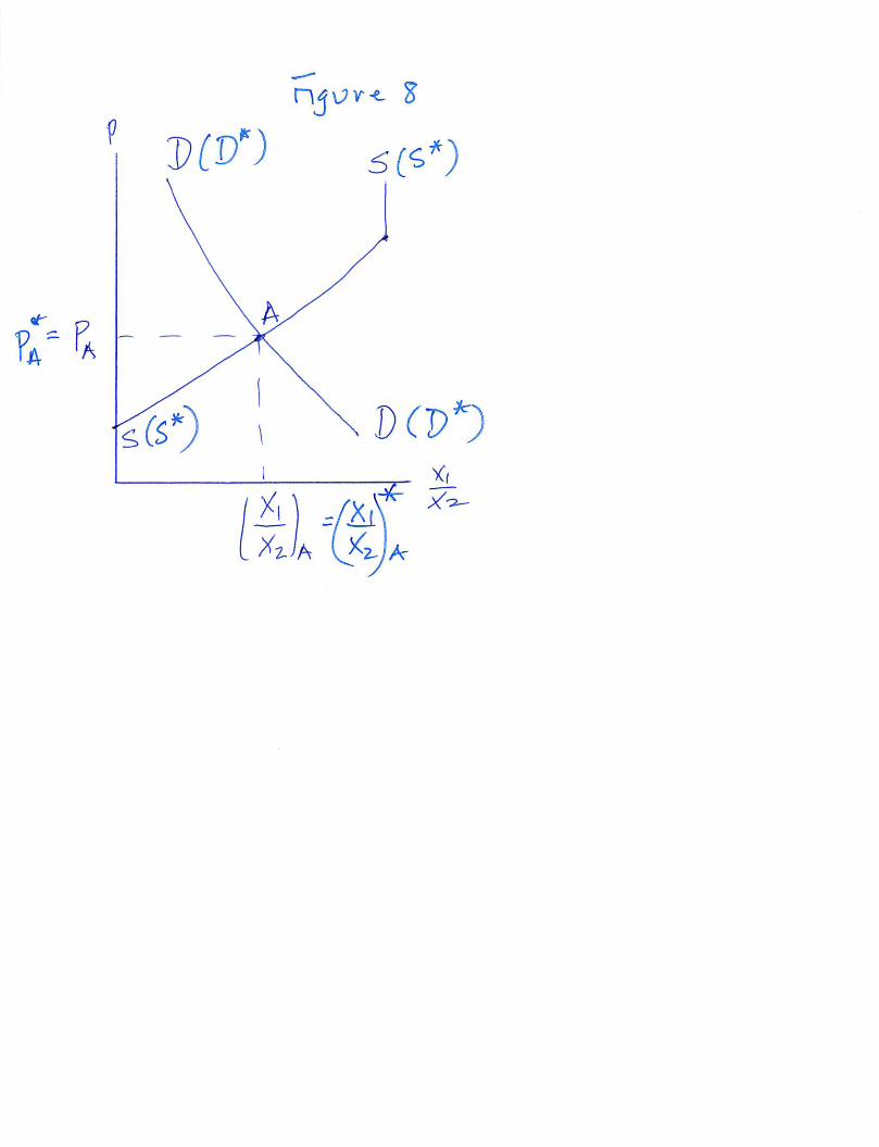
Assume that demand is the same in all countries: At any relative price, the same relative quantities will be demanded in both countries. Let us begin by assuming that not only is demand the same in both countries but so is supply. That is, the two countries are identical.

Insert Figure 8

Thus, a point like A is the same at home and abroad (hence the *s in the figure).

Now, assume The Home country is relatively labour abundant

Now assume that the home country has a higher labour force by – say 10%. We know what this will do to the production possibilities frontier. The Rybczynski line in Figure 6 (a magnification effect) assures us that at any exogenous relative price, the relative supply curve will shift to the right as the labour intensive good will expand relative to the capital intensive good which will decline. Draw the ppf and the Rybczynski line to assure yourself of the story. This has the effect of shifting the relative supply schedule of the home country to the right since relatively more of the labour intensive good, good 1, will be produced at any price ratio. The new autarky equilibrium in the home country is now at B in figure 9

with price pH and output �𝒙𝒙𝑳𝑳𝒙𝒙𝑳𝑳�𝑯𝑯

.

Of course, in the foreign country the autarky price ratio remains at the original price ratio so that relative production remains unchanged at point A.

Insert Figure 9

Looking at the diagram along the home relative supply schedule, it should be clear that the relative price of the labour intensive good pH is cheaper at home than it is abroad. Further, since we are in autarky, our relative output of the labour intensive good is greater than that of the foreign country as well.

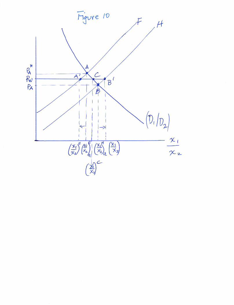
The HO Theorem

Now let trade happen so that there is a common price ratio in Figure 10. We will assume that the world price equilibrium lies between the two autarky prices at pW. What are the consequences? First, notice that countries tend to expand production of the good that intensively uses the factor that is relatively abundant in their country. In the home country this is the labour intensive good, good 1, and production moves from B to B’. In the foreign country, the tendency toward specialization occurs in the capital intensive good, good 2 and production moves from A to A’. Since relative consumption is the same in both countries at point C, clearly the home country must be exporting the labour intensive

11

good, good 1, and the foreign country must be exporting good 2 – the capital intensive good from the relatively capital abundant country.

Insert Figure 10

Factor price equalization

What more can be said? Think about factor prices. Since commodity prices are equalized, we know that with the same technology used by both countries, factor prices (the wages and rental rates) must be the same. In the home country the relative price of good 1 rose increasing the wage and reducing the return to capital. The opposite is try in the foreign country. The relative price of good 2 increased, and consequently the wage fell and the return to capital rose. We know that both countries are better off with trade, but owners of the factors of production both win and lose differently in the two countries.

Trade substitutes for factor mobility

Finally, both country have the equalized factor prices and that is profound. We saw earlier that factor prices signal incentives for factors of production to move between countries. With equalization, no such mobility is necessary. Trade substitutes for factor mobility. Returning to the theme of the great institutions of the late 20th century, by encouraging freer trade, in the context of the HOS model, there was no economic reason for labour to flow across borders since they could earn their marginal products in their own country and these would be the same as in the foreign country. It was no accident that increased trade was associated with higher income, and even more, you could remain at home to receive it.

How has this all worked out in practice?

Empirical Evidence and the HO Theorem

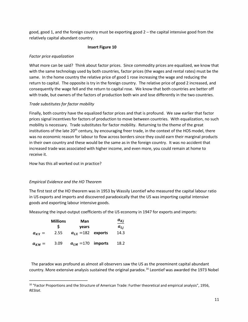
The first test of the HO theorem was in 1953 by Wassily Leontief who measured the capital labour ratio in US exports and imports and discovered paradoxically that the US was importing capital intensive goods and exporting labour intensive goods.

Measuring the input-output coefficients of the US economy in 1947 for exports and imports:

Millions

$ Man years

𝒂𝒂𝑲𝑲𝒊𝒊𝒂𝒂𝑳𝑳𝒊𝒊

𝒂𝒂𝑲𝑲𝑿𝑿 = 2.55 𝒂𝒂𝑳𝑳𝑿𝑿 =182 exports 14.3 𝒂𝒂𝑲𝑲𝑴𝑴 = 3.09 𝒂𝒂𝑳𝑳𝑴𝑴 =170 imports 18.2

The paradox was profound as almost all observers saw the US as the preeminent capital abundant country. More extensive analysis sustained the original paradox.16 Leontief was awarded the 1973 Nobel

16 "Factor Proportions and the Structure of American Trade: Further theoretical and empirical analysis", 1956, REStat.

12

Prize in Economics for his work creating an input-output framework for the US economy and framework that was adopted many countries as part of their calculation of national income and which conveniently adopt for our modelling exercises.

To explain the nature of the paradox, economists have travelled down many intellectual corridors.

1. US was more efficient: US workers 3 are times more efficient than foreign workers: this was Leontief’s preferred explanation. Part of this efficiency is the effect of human capital. Does the US worker embody more capital, or does the worker just have more physical capital to work with?

2. Factor intensity reversal. With many agriculture exports agriculture may be labour-intensive in many countries but capital-intensive in US.

3. There were more factors of production than labour and capital – natural resources or energy, for example.

4. Impediments to trade raise costs in peculiar ways – think how it affected the pattern of trade in Ricardo.

5. If the capital-intensive country has a strong enough taste bias in favour of the capital intensive good, there is no need to export the capital intensive good.

6. Factor market inefficiencies that pay workers differently in different industries so that factor intensity measures are not the same for measuring price responses and output responses.

But economists are nothing if not persistent. A quick search of ECONLIT (February 10, 2018) reports 1,105 articles that mention of Heckscher Ohlin, many of them current. The profound implications of the model and its fundamental division into factors that are accumulated or factors that are current is an attractive tableau for many authors.

The Algebraic Details of the full HOS

So, what does HOS look like when we free up the coefficients of technology?

Recall we have already gotten a great deal from the commodity price-factor price relationship. To explore the flexible coefficients of the model more directly takes us to outputs and factor inputs. Rewriting the labour and capital market constraints we have:

L=aL1x1+aL2x2 K=aK1x1+aK2x2

In looking at these, one way to think about them is as an equilibrium in the labour and capital markets. The left-hand-side (LHS) is the supply of labour, L, that is exogenous, and that the right-hand-side (RHS) is the demands for labour. There is a parallel interpretation of the second equation for capital, K.

The demand for labour is composed of two parts: the demand for labour arising from industry 1, aL1x1, and the demand for labour arising from industry 2, aL2x2. The term aL1x1 tells us that the demand for

13

labour in industry 1 arises from two sources, the scale of output, x1, and the intensity with which labour is used in industry 1: aL1. Clearly a similar deconstruction can be made for capital.

If we ask how do changes in the labour constraint appear, we can differentiate the labour constraint just like we did for prices:

𝑑𝑑𝐿𝐿 = 𝑎𝑎𝐿𝐿1𝑑𝑑𝑥𝑥1 + 𝑥𝑥1𝑑𝑑𝑎𝑎𝐿𝐿1 + 𝑎𝑎𝐿𝐿2𝑑𝑑𝑥𝑥2 + 𝑥𝑥2𝑑𝑑𝑎𝑎𝐿𝐿2

The LHS side is exogenous while the RHS can be rewritten as the scale and intensity effects:

𝑑𝑑𝐿𝐿 = (𝑎𝑎𝐿𝐿1𝑑𝑑𝑥𝑥1 + 𝑎𝑎𝐿𝐿2𝑑𝑑𝑥𝑥2) + (𝑥𝑥1𝑑𝑑𝑎𝑎𝐿𝐿1 + 𝑥𝑥2𝑑𝑑𝑎𝑎𝐿𝐿2)

Because we like to have things in percentage change form we can divide by L, and rearrange:

�𝑑𝑑𝐿𝐿𝐿𝐿� = �𝑎𝑎𝐿𝐿1𝑥𝑥1

𝐿𝐿� �𝑑𝑑𝑥𝑥1

𝑥𝑥1�+ �𝑎𝑎𝐿𝐿2𝑥𝑥2

𝐿𝐿� �𝑑𝑑𝑥𝑥2

𝑥𝑥2� + �𝑎𝑎𝐿𝐿1𝑥𝑥1

𝐿𝐿� �𝑑𝑑𝑎𝑎𝐿𝐿1

𝑎𝑎𝐿𝐿1� + �𝑎𝑎𝐿𝐿2𝑥𝑥2

𝐿𝐿� �𝑑𝑑𝑎𝑎𝐿𝐿2

𝑎𝑎𝐿𝐿2�

The percentage change terms should be obvious, but we put ^’s over them to clarify:

𝐿𝐿� = �𝑎𝑎𝐿𝐿1𝑥𝑥1𝐿𝐿� 𝑥𝑥�1 + �𝑎𝑎𝐿𝐿2𝑥𝑥2

𝐿𝐿� 𝑥𝑥�2 + �𝑎𝑎𝐿𝐿1𝑥𝑥1

𝐿𝐿� 𝑎𝑎�𝐿𝐿1 + �𝑎𝑎𝐿𝐿2𝑥𝑥2

𝐿𝐿� 𝑎𝑎�𝐿𝐿2

So now we need to interpret the terms in parentheses. The first is 𝒂𝒂𝑳𝑳𝑳𝑳𝒙𝒙𝑳𝑳𝑳𝑳

. To understand what this is

recall our definition: 𝒂𝒂𝑳𝑳𝑳𝑳𝒙𝒙𝑳𝑳𝑳𝑳

= �𝑳𝑳𝑳𝑳𝒙𝒙𝑳𝑳� �𝒙𝒙𝑳𝑳

𝑳𝑳� = �𝑳𝑳𝑳𝑳

𝑳𝑳�. So that the bracketed expression is the share of physical

labour used in industry 1. We shall invent a symbol for this which we will call λ.17 We define the share of the labour force used in each industry as 𝝀𝝀𝑳𝑳𝑳𝑳 and 𝝀𝝀𝑳𝑳𝑳𝑳. Our change in the demand for labour then looks like

𝐿𝐿� = [𝜆𝜆𝐿𝐿1 𝑥𝑥�1 + 𝜆𝜆𝐿𝐿2 𝑥𝑥�2] + [𝜆𝜆𝐿𝐿1 𝑎𝑎�𝐿𝐿1 + 𝜆𝜆𝐿𝐿2 𝑎𝑎�𝐿𝐿2]

And we can write a corresponding relation for changes in capital:

𝐾𝐾� = [𝜆𝜆𝐾𝐾1 𝑥𝑥�1 + 𝜆𝜆𝐾𝐾2 𝑥𝑥�2] + [𝜆𝜆𝐾𝐾1 𝑎𝑎�𝐾𝐾1 + 𝜆𝜆𝐾𝐾2 𝑎𝑎�𝐾𝐾2]

Further, 𝝀𝝀𝑳𝑳𝑳𝑳 + 𝝀𝝀𝑳𝑳𝑳𝑳 = 𝑳𝑳 since the total amount of labour is distributed between the two industries, and likewise for capital: 𝝀𝝀𝑲𝑲𝑳𝑳 + 𝝀𝝀𝑲𝑲𝑳𝑳 = 𝑳𝑳.

If the change in the factor intensities were fixed so that all the 𝒂𝒂�𝒊𝒊𝒊𝒊 = 𝟎𝟎, then it is pretty clear that the demand for labour (or capital) depends only on the level of output in the two industries weighted by the share of labour (or capital) used in that industry. This is the first bracketed expression and reflects the scale of output in the industry, the xj’s.

Factor Intensity Changes in Response to Factor Price Changes

If we want to explore the second bracketed term to see how an industry’s demand for (say labour) changes because of changes in the intensity with which labour is used, we need to explore more clearly what goes into each term 𝒂𝒂𝑳𝑳𝒊𝒊. We will begin with 𝒂𝒂�𝑳𝑳𝑳𝑳 and see what influences its changes.

17 Don’t confuse the physical share - the proportion of labour used by each industry, λ – for the distributive share received by factors in the price equation which we called, θ.

14

Recall that the amount of labour used per unit of output can be found along the unit isoquant of Figure 3. The curvature of the isoquant tells us the way in which labour and capital are traded-off as relative factor prices, the wage-rental ratio w/r, changes. This is expressed in the expression for the elasticity of substitution along the isoquant:

𝜎𝜎1 = 𝑎𝑎�𝐾𝐾1−𝑎𝑎�𝐿𝐿1𝑤𝑤�−�̂�𝑟

Or, as we want to isolate 𝒂𝒂�𝑳𝑳𝑳𝑳, we can rewrite it as:

(𝑤𝑤� − �̂�𝑟)𝜎𝜎1 = 𝑎𝑎�𝐾𝐾1 − 𝑎𝑎�𝐿𝐿1

We need to find an expression to reduce the equation to a term in 𝒂𝒂�𝑳𝑳𝑳𝑳. Happily, we have the expression we found with cost minimization:

𝜃𝜃𝐿𝐿1𝑎𝑎�𝐿𝐿1 + 𝜃𝜃𝐾𝐾1𝑎𝑎�𝐾𝐾1 = 0.

Solving for 𝒂𝒂�𝑲𝑲𝑳𝑳 , 𝑎𝑎�𝐾𝐾1 = −(𝜃𝜃𝐿𝐿1𝑎𝑎�𝐿𝐿1)/𝜃𝜃𝐾𝐾1

This lets us solve for 𝒂𝒂�𝑳𝑳𝑳𝑳:

(𝑤𝑤� − �̂�𝑟)𝜎𝜎1 = −𝜃𝜃𝐿𝐿1𝑎𝑎�𝐿𝐿1𝜃𝜃𝐾𝐾1

− 𝑎𝑎�𝐿𝐿1 =−𝜃𝜃𝐿𝐿1𝑎𝑎�𝐿𝐿1 − 𝜃𝜃𝐾𝐾1𝑎𝑎�𝐿𝐿1

𝜃𝜃𝐾𝐾1= −

𝑎𝑎�𝐿𝐿1𝜃𝜃𝐾𝐾1

Or finally solving for 𝒂𝒂�𝑳𝑳𝑳𝑳 as a function of the technology embodied in σ1 when factor prices change, we can see that an increase in the wage-rental ratio reduces the amount of labour hired weighted by the distributive share of capital used:

𝑎𝑎�𝐿𝐿1 = −𝜃𝜃𝐾𝐾1𝜎𝜎1(𝑤𝑤� − �̂�𝑟).

Similarly, we can solve for 𝑎𝑎�𝐿𝐿2:

𝑎𝑎�𝐿𝐿2 = −𝜃𝜃𝐾𝐾2𝜎𝜎2(𝑤𝑤� − �̂�𝑟).

Putting both together gives us the complete expression for the response of labour when output and factor prices change:

𝐿𝐿� = [𝜆𝜆𝐿𝐿1 𝑥𝑥�1 + 𝜆𝜆𝐿𝐿2 𝑥𝑥�2] + [𝜆𝜆𝐿𝐿1 𝑎𝑎�𝐿𝐿1 + 𝜆𝜆𝐿𝐿2 𝑎𝑎�𝐿𝐿2] or

𝐿𝐿� = [𝜆𝜆𝐿𝐿1 𝑥𝑥�1 + 𝜆𝜆𝐿𝐿2 𝑥𝑥�2]− [𝜆𝜆𝐿𝐿1𝜃𝜃𝐾𝐾1𝜎𝜎1(𝑤𝑤� − �̂�𝑟) + 𝜆𝜆𝐿𝐿2𝜃𝜃𝐾𝐾2𝜎𝜎2(𝑤𝑤� − �̂�𝑟)]

But since the (𝑤𝑤� − �̂�𝑟) is in both parts of the expression we can reorganize it slightly so that:

𝐿𝐿� = [𝜆𝜆𝐿𝐿1 𝑥𝑥�1 + 𝜆𝜆𝐿𝐿2 𝑥𝑥�2]− [𝜆𝜆𝐿𝐿1𝜃𝜃𝐾𝐾1𝜎𝜎1 + 𝜆𝜆𝐿𝐿2𝜃𝜃𝐾𝐾2𝜎𝜎2](𝑤𝑤� − �̂�𝑟)

15

What exactly is the second term in brackets that we have worked so hard to find? To figure it out ask “What question does it answer?” Suppose we ignore the first bracketed term. Then the second term answers the question, how does the demand for labour change when the wage rental ratio increases? Or more precisely what is the percentage change in the demand for labour when the wage rate increases relative to the rental rate? It is the economy-wide elasticity of labour demand. To make it easy to read let that whole term be captured by

𝛿𝛿𝐿𝐿 = 𝜆𝜆𝐿𝐿1𝜃𝜃𝐾𝐾1𝜎𝜎1 + 𝜆𝜆𝐿𝐿2𝜃𝜃𝐾𝐾2𝜎𝜎2

So that after all this work we have:

𝐿𝐿� = [𝜆𝜆𝐿𝐿1 𝑥𝑥�1 + 𝜆𝜆𝐿𝐿2 𝑥𝑥�2]− 𝛿𝛿𝐿𝐿(𝑤𝑤� − �̂�𝑟)

With appropriate changes in notation we can write the expression for capital’s percentage change as:

𝐾𝐾� = [𝜆𝜆𝐾𝐾1 𝑥𝑥�1 + 𝜆𝜆𝐾𝐾2 𝑥𝑥�2] + 𝛿𝛿𝐾𝐾(𝑤𝑤� − �̂�𝑟)

In which the only difference is that there is a plus before the wage-rental change. This arises from the observation that the demand for capital increases when the wage-rental ratio rises.

Now, take the difference between the two:

𝐿𝐿� = [𝜆𝜆𝐿𝐿1 𝑥𝑥�1 + 𝜆𝜆𝐿𝐿2 𝑥𝑥�2]− 𝛿𝛿𝐿𝐿(𝑤𝑤� − �̂�𝑟)

- 𝐾𝐾� = [𝜆𝜆𝐾𝐾1 𝑥𝑥�1 + 𝜆𝜆𝐾𝐾2 𝑥𝑥�2] + 𝛿𝛿𝐾𝐾(𝑤𝑤� − �̂�𝑟)

Or,

𝐿𝐿� − 𝐾𝐾� = [(𝜆𝜆𝐿𝐿1 − 𝜆𝜆𝐾𝐾1)𝑥𝑥�1 + (𝜆𝜆𝐿𝐿2 − 𝜆𝜆𝐾𝐾2)𝑥𝑥�2]− (𝛿𝛿𝐿𝐿 + 𝛿𝛿𝐾𝐾)(𝑤𝑤� − �̂�𝑟)

Show that (𝝀𝝀𝑳𝑳𝑳𝑳 − 𝝀𝝀𝑲𝑲𝑳𝑳) = −(𝝀𝝀𝑳𝑳𝑳𝑳 − 𝝀𝝀𝑲𝑲𝑳𝑳) and that 1>(𝝀𝝀𝑳𝑳𝑳𝑳 − 𝝀𝝀𝑲𝑲𝑳𝑳) > 𝟎𝟎.

(Hint: set up the 𝑎𝑎𝐿𝐿2𝑎𝑎𝐾𝐾2

< 𝑎𝑎𝐿𝐿1𝑎𝑎𝐾𝐾1

and then put them in terms of the λ’s, and, manipulate! See Appendix 2)

So that

𝐿𝐿� − 𝐾𝐾� = (𝜆𝜆𝐿𝐿1 − 𝜆𝜆𝐾𝐾1)(𝑥𝑥�1 − 𝑥𝑥�2) − (𝛿𝛿𝐿𝐿 + 𝛿𝛿𝐾𝐾)(𝑤𝑤� − �̂�𝑟)

And rearranging so that relative outputs are being determined:

(𝑥𝑥�1 − 𝑥𝑥�2) =𝐿𝐿� − 𝐾𝐾�

(𝜆𝜆𝐿𝐿1 − 𝜆𝜆𝐾𝐾1)−

(𝛿𝛿𝐿𝐿 + 𝛿𝛿𝐾𝐾)(𝜆𝜆𝐿𝐿1 − 𝜆𝜆𝐾𝐾1)

(𝑤𝑤� − �̂�𝑟)

But we know something about the wage and rental rates. They are determined by exogenous commodity prices. Recall that

(𝑤𝑤� − �̂�𝑟) =�̂�𝑝1 − �̂�𝑝2

(𝜃𝜃𝐿𝐿1 − 𝜃𝜃𝐿𝐿2)

16

Substituting into our expression for

(𝑥𝑥�1 − 𝑥𝑥�2) = 𝐿𝐿�−𝐾𝐾�(𝜆𝜆𝐿𝐿1− 𝜆𝜆𝐾𝐾1)

− { (𝛿𝛿𝐿𝐿+𝛿𝛿𝐾𝐾)(𝜆𝜆𝐿𝐿1− 𝜆𝜆𝐾𝐾1)

1(𝜃𝜃𝐿𝐿1−𝜃𝜃𝐿𝐿2)}(�̂�𝑝1 − �̂�𝑝2)

So, what is the thing on the RHS in the curly-brackets? To answer one must understand the question it answers. Holding endowments constant 𝑳𝑳� − 𝑲𝑲� = 𝟎𝟎, it reports the effect on relative outputs from a change in relative prices. Indeed, it is nothing less that the elasticity of the relative supply curve we derived in Figure 6b which in turn is the elasticity of the production possibilities frontier.

We could rewrite everything we have done so far and simply take all the parameters of the production possibilities frontier and write:

(𝑥𝑥�1 − 𝑥𝑥�2) = 𝐿𝐿�−𝐾𝐾�(𝜆𝜆𝐿𝐿1− 𝜆𝜆𝐾𝐾1)

− {𝜎𝜎𝑆𝑆}(�̂�𝑝1 − �̂�𝑝2)

Notice that at constant relative prices 𝒑𝒑�𝑳𝑳 − 𝒑𝒑�𝑳𝑳 = 𝟎𝟎, since we know that the denominator,

𝑳𝑳 > (𝝀𝝀𝑳𝑳𝑳𝑳 − 𝝀𝝀𝑲𝑲𝑳𝑳 > 𝟎𝟎, then we have our magnification effect along the Rybczynski line.

17

Appendix 1

To show (𝜃𝜃𝐿𝐿1 − 𝜃𝜃𝐿𝐿2) > 0 formally, start with the definition of factor intensity reflecting the relative capital-labour ratios:

𝑎𝑎𝐿𝐿2𝑎𝑎𝐾𝐾2

< 𝑎𝑎𝐿𝐿1𝑎𝑎𝐾𝐾1

Rewrite this in share form by multiplying both sides by w/r:

𝑤𝑤𝑎𝑎𝐿𝐿2𝑟𝑟𝑎𝑎𝐾𝐾2

< 𝑤𝑤𝑎𝑎𝐿𝐿1𝑟𝑟𝑎𝑎𝐾𝐾1

and divide both sides by 1!

𝑤𝑤𝑎𝑎𝐿𝐿2 𝑑𝑑2�𝑟𝑟𝑎𝑎𝐾𝐾2 𝑑𝑑2�

<𝑤𝑤𝑎𝑎𝐿𝐿1 𝑑𝑑1�𝑟𝑟𝑎𝑎𝐾𝐾1 𝑑𝑑1�

So, what are these? Look carefully! What we have is:

𝜃𝜃𝐿𝐿2𝜃𝜃𝐾𝐾2

< 𝜃𝜃𝐿𝐿1𝜃𝜃𝐾𝐾1

or

𝜃𝜃𝐿𝐿2𝜃𝜃𝐾𝐾1 < 𝜃𝜃𝐿𝐿1𝜃𝜃𝐾𝐾2

Using the same substitution as before for 𝜃𝜃𝐾𝐾𝐾𝐾:

𝜃𝜃𝐿𝐿2(1− 𝜃𝜃𝐿𝐿1) < 𝜃𝜃𝐿𝐿1(1− 𝜃𝜃𝐿𝐿2)

Or,

𝜃𝜃𝐿𝐿1 > 𝜃𝜃𝐿𝐿2 or (𝜃𝜃𝐿𝐿1 − 𝜃𝜃𝐿𝐿2) > 0.

Appendix 2

Show that 1> (𝜆𝜆𝐿𝐿1 − 𝜆𝜆𝐾𝐾1) > 0. Again, start with the capital labour ratios:

𝑎𝑎𝐿𝐿2𝑎𝑎𝐾𝐾2

< 𝑎𝑎𝐿𝐿1𝑎𝑎𝐾𝐾1

And this time multiply both sides by (L/K), and then by (x2/x2) on the LHS and (x1/x1) on the RHS:

This gives us

𝑎𝑎𝐿𝐿2𝑥𝑥2𝐿𝐿�

𝑎𝑎𝐾𝐾2𝑥𝑥2𝐾𝐾�

<𝑎𝑎𝐿𝐿1𝑥𝑥1

𝐿𝐿�𝑎𝑎𝐾𝐾1𝑥𝑥1

𝐾𝐾�,

Or,

𝜆𝜆𝐿𝐿2𝜆𝜆𝐾𝐾2

< 𝜆𝜆𝐿𝐿1𝜆𝜆𝐾𝐾1

.

Now this is the same as:

𝜆𝜆𝐿𝐿1𝜆𝜆𝐾𝐾2 > 𝜆𝜆𝐿𝐿2𝜆𝜆𝐾𝐾1

18

And since 𝜆𝜆𝐾𝐾2 = (1 − 𝜆𝜆𝐾𝐾1), and 𝜆𝜆𝐿𝐿2 = 1 − 𝜆𝜆𝐿𝐿1 by substituting in we have:

𝜆𝜆𝐿𝐿1(1− 𝜆𝜆𝐾𝐾1) > (1 − 𝜆𝜆𝐿𝐿1)𝜆𝜆𝐾𝐾1

Or that

𝜆𝜆𝐿𝐿1 > 𝜆𝜆𝐾𝐾1.

Of course, both are fractions and consequently 1 > 𝜆𝜆𝐿𝐿1 − 𝜆𝜆𝐾𝐾1 > 0.