1

The Half-Normal distribution method for measurement error: two case studies

J. Martin Bland Professor of Health Statistics

Department of Health Sciences University of York

Summary Regression methods are used to estimate mean as a continuous function of a predictor variable. We can also estimate standard deviation as a function using the Half-Normal distribution and regression of the absolute values of the residuals. Standard deviation can be estimated as a function either of a different predictor variable of the mean of the index variable itself. Two examples of the application of this in the study of measurement error are given. In one, the analysis is complicated by the presence of a large number of observations where both measurements are zero. In the other, the aim is to estimate the change in measurement error over time with only a single observation on each occasion. This analysis is further complicated by using three different outcome variables in three different small groups of subjects.

Introduction: the Half-Normal method The Half Normal method for dealing with relationships between measurement error and magnitude was introduced by Bland and Altman (1999), based on a suggestion by Altman (1993) for creating centile charts. The method proceeds from the observation that if we have a variable X which follows a Normal distribution with mean zero and variance σ2, the absolute value |X| follows a half-Normal distribution which has mean σπ2 .

This is quite easy to show. The PDF for the Normal and Half-Normal distributions are shown in Figure 1. The PDF for a Half-Normal distribution is

0 if 2

exp22)( 2

2

≥⎟⎟⎠

⎞⎜⎜⎝

⎛−= xxxf

σσπ

= 0 if x < 0

The expected value is given by

dxxxX ∫∞

⎟⎟⎠

⎞⎜⎜⎝

⎛−=

02

2

2exp

22)(E

σσπ

2

0.2

.4.6

.8P

roba

blity

den

sity

-4 -3 -2 -1 0 1 2 3 4Standard deviations

Normal Half-normal

Figure 1. PDFs of the Normal distribution (mean zero) and Half-Normal distribution

This is easy to integrate, because

⎟⎟⎠

⎞⎜⎜⎝

⎛−−=⎟⎟

⎠

⎞⎜⎜⎝

⎛− 2

2

22

2

2exp

2exp

σσσxxx

dxd

so

( )

[ ]

σπ

σπ

σσπσ

σσ

σπσσπ

2

102

2exp

22

2exp

22

2exp

22

0

22

02

22

02

2

=

−−=

⎥⎦

⎤⎢⎣

⎡⎟⎟⎠

⎞⎜⎜⎝

⎛−

−=

⎟⎟⎠

⎞⎜⎜⎝

⎛−−=⎟⎟

⎠

⎞⎜⎜⎝

⎛−

∞

∞∞

∫∫

x

dxxdxddxxx

Altman (1993) proposed that when both mean and standard deviation of an outcome variable change with a predictor, as for example for fetal measurements varying with gestational age, one could regress the outcome on the predictor to find a model for the mean, then regress the absolute residual about this regression on the predictor to model the standard deviation. We then multiply the fitted value by 2π to obtain the predicted standard deviation of the outcome variable.

Bland and Altman (1999) used this approach in the study of agreement between methods of measurement. They wanted to calculate 95% limits of agreement (Altman and Bland 1983, Bland and Altman 1986) for observations by two different methods of measurement. In the simple method, we estimate these by sd 96.1± , where d is the mean difference between observations by the two methods and s is the standard deviation of differences. We assume that the differences between pairs of observations are independent of the magnitude of the

3

variable being measured. We check this by plotting the difference against the average of the two observations, as the best estimate of magnitude for that subject. If we cannot assume independence, we can use the Half-Normal method to predict the mean and standard deviation of the differences from the magnitude, the average of the two observations, then estimate the 95% limits of agreement for any given magnitude. In practice, we would then use the observed value for a measurement by one method as an estimate of the magnitude to give limits within which an observation by the other would be expected to lie.

The Half-Normal method provides a powerful and simple method for estimating measurement error which is neither constant nor proportional to magnitude. In this paper I describe two case studies. In the first, data with an very large number of zeros is analysed, in the other the researcher wanted to know whether there was evidence of a change in measurement error over time, despite having only a single observation on each occasion.

Regression on magnitude and dealing with zeros This problem (Sevrukov et al. 2004??) came from Alex Sevrukov of University of Illinois College of Medicine, Chicago. He approached me for help in November 2003, as follows:

“I am currently working on a study of repeatability of quantitative electron-beam CT measurement of coronary artery calcium (CAC). There has been only a single study by Bielak et al. (2001) that addressed this critical issue by use of the limits of agreement but they fell short of producing results that could be applicable in clinical practice. And this is exactly my goal for the analysis I am conducting on 2,217 pairs of repeated measurements of CAC.

“I would greatly appreciate if you gave a working example of estimating the measurement error in a sample of pairs of repeated measurements where the difference (D) is not related to the average (A) of the two CAC measurements (the mean difference is zero since the same method was used), and SD increases as the magnitude of the measurement increases (exactly the situation with CAC). The example on comparing two methods for measuring the fat content of milk in your 1999 article in the Statistical Methods in Medical Research was very useful but it did not address repeatability per se.”

He had a large sample of measurements of coronary artery calcium where variability clearly increased with magnitude. Figure 2 shows a plot of the difference between the pairs against the average.

The first step was to carryout the regressions. As the two measurements are replicates there should be no systematic difference between them and the mean difference between replicates should be zero. For any given magnitude of CAC, the differences can therefore be assumed to follow a Normal distribution with mean zero. The absolute value of the difference should have a Half-Normal distribution.

4

-200

-100

010

020

0D

iffer

ence

0 500 1000 1500 2000Average CAC, Agatston

Figure 2. Difference versus mean plot for pairs of measurements of coronary calcium.

-300

-200

-100

010

020

030

0D

iffer

ence

0 500 1000 1500 2000Average CAC, Agatston

95% limits

Figure 3. Limits calculated from the fractional polynomial model.

5

-200

-100

010

020

0D

iffer

ence

0 500 1000 1500 2000Average CAC, Agatston

95% limits

Figure 4. Limits calculated from the regression on root CAC.

Table 1. Fit of different models for predicting the absolute difference from average of two CAC measurements. Residual sum of

squares Degrees of freedom Residual variance

Fractional polynomial 406127 2214 183.4 Simple regression on √CAC

414106 2215 187.0

Zero intercept regression on √CAC

415573 2216 187.5

I wanted to find the best predictor of the absolute difference from magnitude, as represented by the average of the two measurements. As this relationship was clearly non-linear from Figure 2, I used the fractional polynomial method of Royston and Altman (1994). This gave

Abdiff = -0.04632 + 1.488 √CAC+ 0.02393 CAC

The resulting limits, calculated by multiplying the predicted absolute difference by 2/96.1 π , are shown in Figure 3 and appear to fit the data well. These are the limits

estimated to contain 95% of pairs of measurements of CAC, hence if a subject has successive measurements which differ by more than this it would suggest that the subject’s CAC has changed rather than being the result of measurement error. Inspection of the equation suggested that we could omit the final term and fit a simple function of √CAC, so I did this. I obtained

Abdiff = -0.9733 + 2.067 √CAC

6

-20

-10

010

20D

iffer

ence

0 2 4 6 8 10Average CAC, Agatston

95% limits

Figure 5. Limits calculated from the regression on root CAC, for average CAC < 10.

-200

-100

010

020

0D

iffer

ence

0 500 1000 1500 2000Average CAC, Agatston

95% limits

Figure 6. Limits calculated from the regression on root CAC with zero intercept.

7

-20

-10

010

20D

iffer

ence

0 2 4 6 8 10Average CAC, Agatston

95% limits

Figure 7. Limits calculated from the regression on root CAC with zero intercept, for average CAC < 10.

The resulting limits are shown in Figure 4. The fit looks almost as good as Figure 3, although the limits are noticeably narrower for high CAC. The residual sums of squares and variances are very similar (Table 1).

I accordingly decided to adopt this simpler model and checked its coverage. I expected to find about 2.5% of differences above the upper limit and 2.5% below the lower limit. To my surprise, I found that 1.6% of differences were above the upper limit, not too bad, but 50.6% were below the lower limit. Inspection of the region of Figure 4 close to zero CAC (Figure 5) shows that this arose because the limits produced a negative estimated standard deviation at zero, the limit curves crossing the CAC axis at 0.22.

There is a very large number of observations with both measurements equal to zero; 1097, 49% of all observations. Thus that one point on Figure 5 at CAC = 0 actually represents 1097 superimposed points. Limiting the check to observations with at least one of the measurements non-zero produced an acceptable 2.5% of observations below the lower limit and 3.4% above the upper one. However, the model was clearly inadequate as the absolute residual, and hence the standard deviation, should not be predicted to be negative.

One possible solution was to constrain the model to produce non-zero estimates by forcing the constant term to be zero. It is very small at minus one, given that CAC ranges from zero to 1846.8 Agatston units. Doing this gave the equation

Abdiff = 2.007 √CAC

The resulting limits are shown in Figure 6 and for small CAC in Figure 7. The fit is almost as good as the previous models (Table 1). For these limits, there are 0.9% of differences

8

Table 2. Distribution of non-zero CAC when the other CAC is zero (Agatston units). Non-zero CAC

Frequency Relative frequency

0.5 3 2.7%0.8 12 13.3%1.0 13 24.8%1.3 11 34.5%1.5 10 43.4%1.8 4 46.9%2.0 1 47.8%2.1 4 51.3%2.3 4 54.9%2.6 5 59.3%2.8 2 61.1%2.9 1 62.0%3.1 4 65.5%3.3 1 66.4%3.4 2 68.1%3.6 2 69.9%3.9 2 71.7%4.1 2 73.5%4.3 1 74.3%4.6 1 75.2%5.1 1 76.1%5.2 3 78.8%5.5 1 79.7%5.7 3 82.3%6.2 1 83.2%6.7 4 86.7%7.1 1 87.6%7.2 1 88.5%7.7 1 89.4%9.1 1 90.3%9.3 2 92.0%9.5 1 92.9%

10.1 1 93.8%10.2 1 94.7%11.6 1 95.6%12.4 1 96.5%12.9 1 97.4%14.7 2 99.1%19.3 1 100.0%

Total 113 100.0%

below the lower limit and 1.1% above the upper. If we restrict attention to the 1,007 observations with at least one non-zero observation, 1.8% of differences are below the lower limit and 2.1% above the upper limit, giving us 96.1% of differences between the limits compared to the 95% which we would like.

The equation for the limits is found by multiplying the coefficient by 2/96.1 π , giving

9

Limit = ±4.930 √CAC

The 95% confidence interval for the limits coefficient is 4.773 to 5.087 Agatston units, so the limits are well estimated.

The final question was: what do we do when the observation is zero? The limits would be zero too, which is clearly wrong. As this was a convenience sample formed by assembling a set with non-zero observations and adding an arbitrary number of zero observations to the data, we cannot estimate the probability of a second observation being zero given that the first is. The sample is not representative. However, we can estimate the distribution for the second observation given that it is non-zero. A subsample was assembled of observations with one zero and one non-zero observation. The distribution for the non-zero observation is shown in Table 2.

The 95th centile for this distribution is at observation 113×0.95 = 107.35. We could simply round this up and take the 108th observation, the observation being 11.6. For the 95% confidence interval using the Binomial method, we need the observations at rank

05.095.011396.195.0113 ××±× = 102.8 to 111.9. Hence we can take the 103rd and 112th observations, to 9.3 to 14.7. For convenience we can round these to integers. Hence if we have an observation of zero, should a second CAC be non-zero it is unlikely to be above 12 Agatston units, 95% CI 9 to 15 units.

We were able to conclude that if a patient’s CAC is measured, in the absence of a real change in CAC a second measurement is likely to be within ±4.930 √CAC of the first for a non zero measurement. If the measurement is zero, the second in likely to be zero also, and if not is likely to be below 12 Agatston units.

Two earlier studies had presented data similar to those described here. Bielak et al. (2001) also used the Half-Normal method, but they used a linear fit. This appeared to give limits which are too wide for low CAC and too narrow for high CAC. Hokanson et al. (2004) stabilised the variance by square root transformation. Their estimate of repeatability was thus the same for all levels of CAC but was in square root units. We think that a non-constant, but easily calculated estimate in the same units of the measurement is of more use to busy clinicians.

Regression on time The second problem came from Christopher Askew of the School of Medicine, University of Queensland, Brisbane, in February 2004. He wrote:

“I have conducted a small pilot study to investigate the effect of repeated testing (practice tests if you like) on the within subject variability of various exercise tests.

“DESIGN: 15 patients with Peripheral Arterial Disease were randomised to either: a treadmill test group, a cycle test group, or a calf test group. Each subject completed the respective test once per week for eight weeks.

“MAIN HYPOTHESIS: With repeated testing, the variability of test performance on each test modality would decrease.”

He had tried many ways to examine this hypothesis, without success, and finished:

“I would be very grateful for any advice you are able to give.”

10

400

500

600

400

500

600

400

500

600

400

500

600

400

500

600

1 2 3 4 5 6 7 8 1 2 3 4 5 6 7 8 1 2 3 4 5 6 7 8

1 2 3 4 5 6 7 8 1 2 3 4 5 6 7 8

Subject A Subject B Subject C

Subject D Subject E

Cyc

le ti

me

(s)

Week

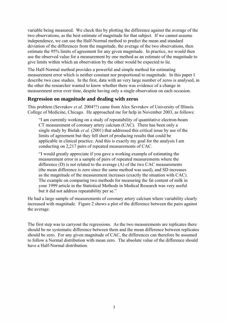
Figure 8. Cycle times over 8 weeks for 5 subjects.

400

500

600

400

500

600

400

500

600

400

500

600

400

500

600

1 2 3 4 5 6 7 8 1 2 3 4 5 6 7 8 1 2 3 4 5 6 7 8

1 2 3 4 5 6 7 8 1 2 3 4 5 6 7 8

Subject A Subject B Subject C

Subject D Subject E

Cycle time (s) Fitted values

Week

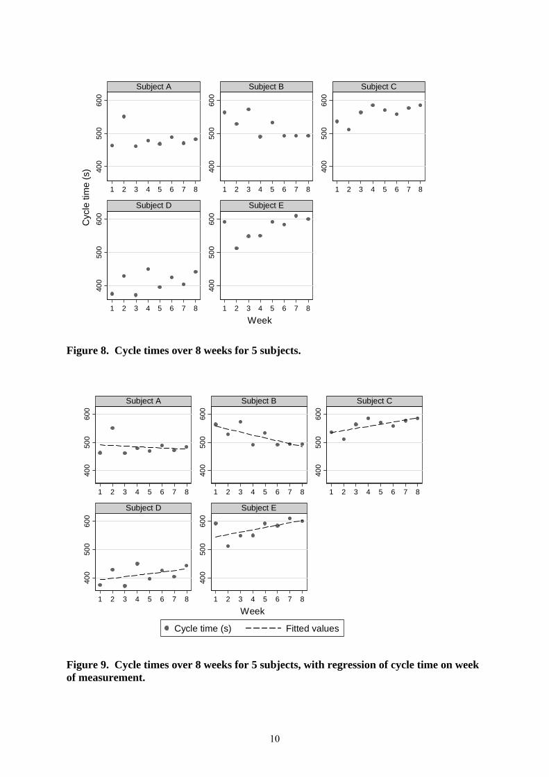
Figure 9. Cycle times over 8 weeks for 5 subjects, with regression of cycle time on week of measurement.

11

-50

050

-50

050

-50

050

-50

050

-50

050

1 2 3 4 5 6 7 8 1 2 3 4 5 6 7 8 1 2 3 4 5 6 7 8

1 2 3 4 5 6 7 8 1 2 3 4 5 6 7 8

Subject A Subject B Subject C

Subject D Subject E

Res

idua

l

Week

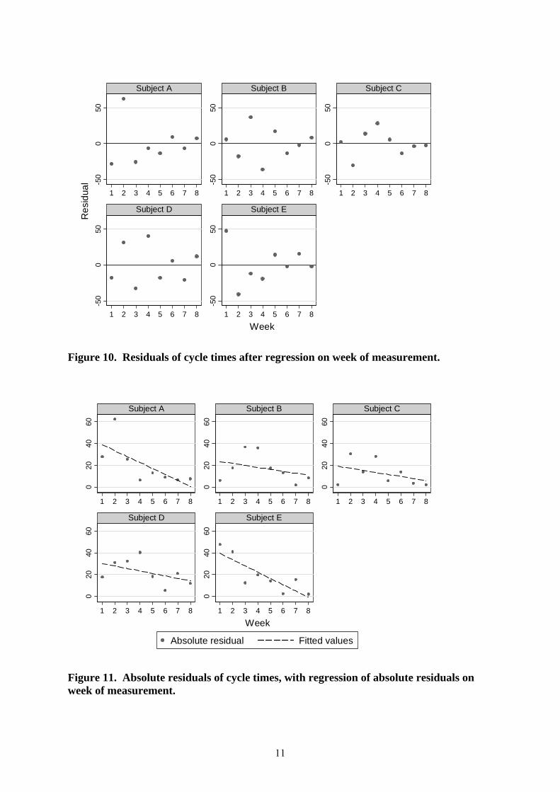
Figure 10. Residuals of cycle times after regression on week of measurement.

020

4060

020

4060

020

4060

020

4060

020

4060

1 2 3 4 5 6 7 8 1 2 3 4 5 6 7 8 1 2 3 4 5 6 7 8

1 2 3 4 5 6 7 8 1 2 3 4 5 6 7 8

Subject A Subject B Subject C

Subject D Subject E

Absolute residual Fitted values

Week

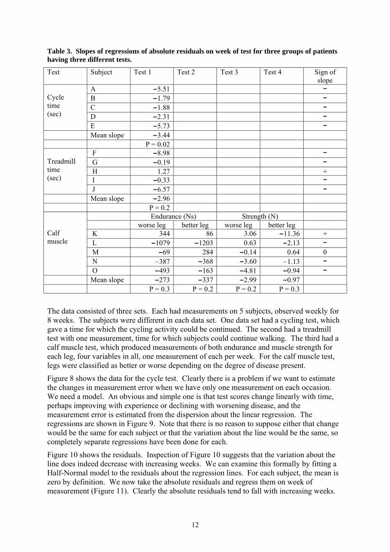
Figure 11. Absolute residuals of cycle times, with regression of absolute residuals on week of measurement.

12

Table 3. Slopes of regressions of absolute residuals on week of test for three groups of patients having three different tests.

Test Subject Test 1 Test 2 Test 3 Test 4 Sign of slope

A -5.51 - B -1.79 - C -1.88 - D -2.31 -

Cycle time (sec)

E -5.73 - Mean slope -3.44 P = 0.02

F -8.98 - G -0.19 - H 1.27 + I -0.33 -

Treadmill time (sec)

J -6.57 - Mean slope -2.96 P = 0.2

Endurance (Ns) Strength (N) worse leg better leg worse leg better leg K 344 86 3.06 -11.36 + L -1079 -1203 0.63 -2.13 - M -69 284 -0.14 0.64 0 N -387 -368 -3.60 -1.13 -

Calf muscle

O -493 -163 -4.81 -0.94 - Mean slope -273 -337 –2.99 –0.97 P = 0.3 P = 0.2 P = 0.2 P = 0.3 The data consisted of three sets. Each had measurements on 5 subjects, observed weekly for 8 weeks. The subjects were different in each data set. One data set had a cycling test, which gave a time for which the cycling activity could be continued. The second had a treadmill test with one measurement, time for which subjects could continue walking. The third had a calf muscle test, which produced measurements of both endurance and muscle strength for each leg, four variables in all, one measurement of each per week. For the calf muscle test, legs were classified as better or worse depending on the degree of disease present.

Figure 8 shows the data for the cycle test. Clearly there is a problem if we want to estimate the changes in measurement error when we have only one measurement on each occasion. We need a model. An obvious and simple one is that test scores change linearly with time, perhaps improving with experience or declining with worsening disease, and the measurement error is estimated from the dispersion about the linear regression. The regressions are shown in Figure 9. Note that there is no reason to suppose either that change would be the same for each subject or that the variation about the line would be the same, so completely separate regressions have been done for each.

Figure 10 shows the residuals. Inspection of Figure 10 suggests that the variation about the line does indeed decrease with increasing weeks. We can examine this formally by fitting a Half-Normal model to the residuals about the regression lines. For each subject, the mean is zero by definition. We now take the absolute residuals and regress them on week of measurement (Figure 11). Clearly the absolute residuals tend to fall with increasing weeks.

13

All subjects appear to show a decrease in variability. The five slopes are -5.51, -1.79, -2.31 -1.88, -2.31, and -5.73. The mean slope is -3.44 (95% CI -5.92 to -0.96, P= 0.02). We can convert absolute residual to standard deviation by multiplying by 2/π . The mean slope thus corresponds to a fall in standard deviation of 4.3 seconds per week (95% CI 1.2 to 7.4 sec/week).

The analysis for the other data proceeds in the same way. Not all variables gave results which were as clear as for cycle time. They are summarised in Table 3. None of the other variables showed statistical significance.

Finally, we wanted to provided a combined test of the null hypothesis that measurement error did not change with weeks. We have tests on three groups of 5 subjects. The cycle test and treadmill test groups each produced one slope of standard deviation against week. The calf muscle test group produced four slopes, endurance and strength for each leg. We would like to combine the data to get a common test of the null hypothesis that the direction of the slope is zero whatever the test, against the alternative that there is a consistent trend in the same direction.

There are two problems:

1. the tests give data which are in different units and so the slopes are in different units and cannot be combined directly,

2. the calf muscle test produces four different slopes for each subject.

Problem 1 is solved by using the sign test. We look at the direction of the slopes only. If the null hypothesis were true, the probability that a slope is positive = probability that a slope is negative.

Problem 2 is solved by taking the majority direction. If a subject has 3 or 4 slopes in the same direction, that is the direction for that subject. If a subject has 2 slopes in each direction, it scores zero and contributes no information.

The signs are shown in Table 3. We have 12 negative slopes, 2 positive slopes, 1 slope without any direction. The sign test gives P=0.01 for a two-sided test.

We were able to conclude that variability of performance, i.e. measurement error, tends to decrease with practice. It is not possible to say how this varies from test to test given the small number of subjects.

Discussion These case studies illustrate both the utility of the Half-Normal distribution method and the variety of problems which arise in the study of measurement error.

The Half-Normal method may not be optimum, in that regression of absolute residuals on either magnitude or some other variable, such as time, ignores the clearly non-Normal nature of the errors about the regression. It may thus be biased. However, in practice it appears to give quite good coverage for the distribution of the observed differences and it has the great advantage of being easy to understand and simple to carry out.

Studies in this area are often done by researchers with little access to statisticians. As a result, errors in the interpretation of statistical analyses such as correlation and regression occur frequently (Altman and Bland 1983; Bland and Altman 1986, 2003). There is a great need for simple and transparent statistical methods, which researchers from other disciplines can apply to their data using standard software. Although the analyses here may have

14

required a facility with statistical thinking which could not be expected from scientists in other disciplines, they were readily understood by the collaborators.

Acknowledgements I would like to thank Alex Sevrukov and Christopher Askew for bringing these problems to my attention and for two very stimulating, fruitful, and enjoyable collaborations.

References Altman DG, Bland JM. Measurement in medicine: the analysis of method comparison studies. The Statistician 1983; 32: 307-317.

Altman DG. Construction of age-related reference centiles using absolute residuals. Stat Med. 1993; 12: 917-924.

Askew CD, Green S, Bland JM, Kerr GK, Walker PJ. Test familiarisation reduces performance variability in Peripheral Arterial Disease. Medicine and Science in Sport and Exercise, in press we hope.

Bielak LF, Sheedy PF 2nd, Peyser PA. Coronary artery calcification measured at electron-beam CT: agreement in dual scan runs and change over time. Radiology. 2001; 218: 224-229.

Bland JM, Altman DG. Measuring agreement in method comparison studies. Stat Methods Med Res. 1999; 8: 135-160.

Bland JM, Altman DG. Applying the right statistics: analyses of measurement studies. Ultrasound Obstet Gynecol. 2003; 22: 85-93.

Bland JM, Altman DG. Statistical methods for assessing agreement between two methods of clinical measurement. Lancet. 1986; i: 307-310.

Hokanson JE,T MacKenzie T, Kinney G, Snell-Bergeon JK, Dabelea D, Ehrlich J, Eckel RH, Rewers M. Evaluating changes in coronary artery calcium: an analytic method that accounts for interscan variability. American Journal of Radiology 2004; 182: 1327–1332.

Royston P, Altman DG. Regression using fractional polynomials of continuous covariates - parsimonious parametric modelling. Applied Statistics-Journal of the Royal Statistical Society Series C 1994; 43: 429-467.

Sevrukov A, Bland JM. Serial [quantitative] electron-beam CT of coronary artery calcium: from variability between repeated measurements to long-term changes. Radiology, in press we hope.