the future of oil: geology versus technology...
TRANSCRIPT
International Journal of Forecasting 31 (2015) 207–221
Contents lists available at ScienceDirect
International Journal of Forecasting
journal homepage: www.elsevier.com/locate/ijforecast
The future of oil: Geology versus technology✩
Jaromir Benes a, Marcelle Chauvet b,∗, Ondra Kamenik c,1,2, Michael Kumhof a,Douglas Laxton a, Susanna Mursula a, Jack Selody d,1,3
a International Monetary Fund, United Statesb University of California Riverside, United Statesc OGResearch, Czech Republicd Promontory Financial Group, Canada
a r t i c l e i n f o
Keywords:Exhaustible resourcesFossil fuelsOil depletionHubbert’s peak oilBayesian econometrics
a b s t r a c t
We discuss and reconcile the geological and economic/technological views concerning thefuture of world oil production and prices, and present a nonlinear econometric model ofthe world oil market that encompasses both views. The model performs far better thanexisting empirical models in forecasting oil prices and oil output out-of-sample. Its pointforecast is for a near doubling of the real price of oil over the coming decade, though theerror bands are wide, reflecting sharply differing judgments on the ultimately recoverablereserves, and on future price elasticities of oil demand and supply.© 2014 International Institute of Forecasters. Published by Elsevier B.V. All rights reserved.
ier
1. Introduction
Future real oil prices are notoriously difficult to pre-dict in real time, particularly over the medium and longrun. Economists, government officials, and market oil spe-cialists all experience this first hand, generally obtainingoil price forecasts that display no improvement, or only a
✩ The views expressed here are those of the authors, and do notnecessarily reflect the position of the International Monetary Fund or anyother institution with which the authors are affiliated.∗ Correspondence to: Department of Economics, University of Califor-
nia Riverside, CA 92521, United States. Tel.: +1 951 827 1587.E-mail addresses: [email protected] (J. Benes), [email protected]
(M. Chauvet), [email protected] (O. Kamenik),[email protected] (M. Kumhof), [email protected] (D. Laxton),[email protected] (S. Mursula), [email protected] (J. Selody).1 Research Department, International Monetary Fund, 700 19th St NW,
Washington, DC 20431, United States.2 Present address: OGResearch, Sibeliova 41, Prague 6, 16200, Czech
Republic.3 Present address: Promontory Financial Group, Toronto, Canada. Tel.:
+1 416 863 8500.
http://dx.doi.org/10.1016/j.ijforecast.2014.03.0120169-2070/© 2014 International Institute of Forecasters. Published by Elsev
marginal improvement, over the no-change forecast. How-ever, the no-change forecast itself does a very poor job ofpredicting oil prices. This is particularly the case duringsharp increases in prices, such as in the mid-1970s andthe 2000s, together with the abrupt oscillations during theGreat Recession in 2007–2009, which professional fore-casters were slow to recognize. This result is well-knownwithin the oil industry and the academic literature.
Several papers have shown, however, that the real priceoil has some predictability in the short run. In a recent pa-per, Alquist, Kilian, and Vigfusson (2013) report that out-of-sample monthly forecasts from a reduced-form vectorautoregressive model (VAR) of the global oil market aremore reliable than forecasts from the random walk modelat short horizons.4 Nevertheless, at medium and long
4 The forecasting performance is sensitive to variable selection and thelag length. In particular, Alquist et al. (2013) find, like Baumeister andKilian (2012), that the real price of oil, defined as US refiners’ acquisitioncost for imported crude oil, is easier to forecast than the real price ofWest Texas Intermediate (WTI) crude oil. These results are based onmeansquare predictive errors.
B.V. All rights reserved.
208 J. Benes et al. / International Journal of Forecasting 31 (2015) 207–221
horizons of one year and above, no-change forecasts sys-tematically beat all models studied, and also professionalforecasters. This result is also found by Baumeister and Kil-ian (2012, in press), who extend the analysis to include realtime forecast restrictions at themonthly and quarterly fre-quencies, respectively. The econometric models of Alquistet al. (2013) and Baumeister and Kilian (2012, in press) usemacroeconomic and financial indicators, as well as globalcrude oil production, as predictors of future oil prices.Many of these indicators are highly correlated with fluctu-ations in aggregate demand, so that the forecasts capturechanges in the price of oil caused by variations in demand.In order to identify the roles of oil demand and oil supplyshocks, Kilian (2009) proposes a structural VAR model ofthe global crude oil market. The model distinguishes be-tween three drivers of real oil prices: global demand forindustrial commodities, precautionary demand for oil, andoil supply, with the latter capturing the possibility of sup-ply disruptions due to political events in oil producers, thedominant supply shock in historical data. The paper findsthat the two demand shocks have been very important asdrivers of oil prices, while supply shocks have had a negli-gible effect.
However, there is an alternative explanation for therecent persistent price movements that has received verylittle attention in the economics literature, despite therebeing considerable evidence to support it. This is the ideathat one key driver of recent eventsmay have been a highlypersistent or even permanent shock to oil production thatis due to geological limits on the oil industry’s ability tomaintain the historical growth rate of production. Theextent to which the literature discounts or embraces thispossibility is critical for its interpretation of recent eventsin the oil markets.5
The most prominent economist who does not discountthis possibility is James Hamilton. Hamilton (2009) findsthat temporary disruptions in physical oil production havealready played a major role in explaining the historical dy-namics of oil price movements. Furthermore, he arguesthat stagnating world oil production, meaning a very per-sistent reduction in the growth rate of oil production, mayhave been one of the reasons for the run-up in oil pricesin 2007–08.6 According to Hamilton (2009), the main rea-sons why oil supply shocks affect output is their disruptiveeffects on key industries such as automotive manufactur-ing, and their impact on consumers’ disposable incomes. Inother words, the main effect is on the aggregate demand.As for aggregate supply effects, there may be large short-run impacts due to very low short-run elasticities of sub-stitution between oil and other factors of production. It isoften argued that such elasticities of substitution would
5 Kilian’s (2009) analysis does not consider the possibility of shocks tothe supply of oil that are driven by terminal geological limits.6 In particular, Hamilton (2009) argues that the main dynamic was
strong demand, at a low price elasticity of demand, meeting stagnatingworld oil production. Hamilton also finds that the flow of investmentdollars into commodity futures contracts was important, but not the keyfactor, in explaining the late 2000s increase in real oil prices, the largestin history. By contrast, Baumeister and Peersman (2013), Kilian (2008,2009), and Kilian and Hicks (2013) stress the role of oil demand shocksrather than oil supply shocks in causing the 2007–2008 oil price surge.
tend to get larger over longer horizons, as agents find pos-sible substitutes for oil, fueled by high prices that stimulatethe technological change that can increase both the recov-ery of oil and the availability of substitutes for oil. Hamilton(2013), however, argues that the main reason for the his-toric growth in oil production has been the exploration ofnew geographic areas, rather than the application of bet-ter technology to existing sources, and that the end of thatera could come soon. His paper goes on to explore the po-tentially very problematic implications of a slower futuregrowth in oil production for future GDP growth.
Other than Hamilton, most proponents of the geolog-ical view of future oil production are found among phys-ical scientists. They argue that oil reserves are ultimatelyfinite, easy-to-access oil is produced first, and therefore,oil must become harder and more expensive to produceas the cumulated amount of oil already produced grows.According tomany scientists in this group, the recently ob-served stagnation in oil production in the face of persistentand large oil price increases is a sign that a physical scarcityof oil is already here, or at least is imminent, and thatit must eventually overwhelm the stimulative effects ofhigher prices. Furthermore, based on extensive studies ofalternative technologies and resources, they state that suit-able substitutes for oil simply do not exist on the requiredscale, and that technologies for improving oil recoverymust eventually run into limits dictated by the laws ofthermodynamics, specifically entropy.
This view of oil production has its origins in the workof the geoscientist Hubbert (1956, 1962, 1967). Hubbert(1956) fitted historical production data to a symmetricbell-shaped curve and predicted correctly that US oil pro-ductionwould peak in 1970. Subsequently, Hubbert (1962,1967) projected the ultimate quantity of oil to be recov-ered, and the rate at which it would be produced in thelower 48 US states. Hubbert (1962) adjusted logistic curvesto cumulative production and discoveries, while Hubbert(1967) proposed an analysis of the quantity of oil discov-ered per foot of well drilled (yield per effort, YPE), fitting anegative exponential in order to form forecasts of the ul-timate oil recovery (UOC). Hubbert’s gloomy projectionsboth spurred awareness and attracted criticism from theoil industry, government agencies, and academics. Some ofthe criticismswere related to the fact that themodels wereonly based on physical oil production and discovery, andignored the role of economics and technological changes.The response of Hubbert, and of subsequent studies val-idating his work, was that geological features were ulti-mately the main drivers of oil discovery, production anddistribution, and that factors other than thosewere alreadyembedded in the historical series used in the model.
The empirical success of Hubbert’s seminal approachmotivated various important academic studies that incor-porated additional economic, institutional and/or techno-logical factors into the original model, and that proposedalternative estimation methods. A partial list includes thestudies by Cleveland and Kaufmann (1991), Kaufmann(1991), Kaufmann and Cleveland (2001), and Pesaran andSamiei (1995). Cleveland and Kaufmann (1991) extendHubbert’s (1962) model to account for the non-randomhistorical drilling pattern in the oil industry in the lower

J. Benes et al. / International Journal of Forecasting 31 (2015) 207–221 209
48 US states, and to incorporate the effects of the realprice of oil and the annual rate of drilling effort on theYPE. The analysis is also extended to account for politi-cal/institutional factors, such as pro-rationing by the TexasRailroad Commission (TRC). The model is based on an ex-tended version of Hubbert’s production curve, and is esti-mated via ordinary least squares (OLS). Kaufmann (1991)proposes a two-step approach to study the impact of ge-ological, economic, and political/institutional changes onoil production in the lower 48 states. It combines Hub-bert’s fitting approach with econometric methods. In thefirst stage, changes in physical resources are representedby a bell-shaped curve. In the second stage, the differ-ence between actual and estimated production is mod-eled as a function of political/institutional and economicfactors: average real oil prices, the relative price of oil tonatural gas, and pro-rationing by the TRC. This model isestimated using OLS, and a grid search is used to iden-tify the bell-shaped curves from the two-step procedure.Kaufmann and Cleveland (2001) argue that the forecastsuccess of Hubbert’s bell-shaped curve is due to the factthat it is a good approximation of the nonlinear long-run oil cost function. However, Kaufmann and Cleveland(2001) claim that Hubbert’s results might be spurious be-cause he does not take into account stochastic trendswhich are shared by oil production and other variables ofthe model. Their paper proposes a vector error correctionmodel of oil production that includes real oil prices, av-erage cost of production, and pro-rationing by the TRC.7Essentially, the analysis allows for economic factors (oilprices) and institutional factors (decisions from the TRC)having an impact on the dynamics of oil production. Pe-saran and Samiei (1995) evaluate alternative estimationmethods for the model of Hubbert (1956, 1962, 1967) andfor the extensions of Cleveland and Kaufmann (1991) andKaufmann (1991). The paper discusses parameter iden-tification and estimation of the models, and proposes aforecasting formula for the ultimate oil recovery basedon the rate of recovery rather than the cumulative pro-duction function.8 The paper argues that when economicfactors are taken into account, the estimates of ultimaterecovery become state-dependent. Themodel is estimatedfor the lower 48 US states under this assumption.
More recently, Hubbert’s work was discussed in a studyfor the US Department of Energy by Hirsch, Bezdek, andWendling (2005), and in a subsequent book by Hirsch,Bezdek, and Wendling (2010).9 The most thorough re-search available on this topic is by the UK Energy ResearchCentre (2009), and is summarized succinctly by Sorrell,Miller, Bentley, and Speirs (2010). Based on a wealth of ge-ological and engineering evidence, these authors conclude
7 In their analysis, real oil prices are decomposed to account forasymmetric effects of price increases. In addition, the inclusion of theaverage cost of production implies that firms do not rank and producetheir fields as a function of quality.8 These problems in identification and estimation of the models would
cast doubt in Kaufmann and Cleveland’s (2001) results.9 Other studies by official US agencies that havewarned about this issue
include studies by the Government Accountability Office (2007) and theUnited States Joint Forces Command (2010).
that there is a significant risk of a peak in conventional oilproduction before 2020, with an inexorable decline there-after.
In this paper we find that our ability to forecast futuredevelopments in the oil market, and therefore, by impli-cation, in aggregate activity, can be improved dramaticallyby combining the geological and economic/technologicalviews of oil production, and by estimating their respec-tive contributions.10 We develop a simple macroeconomicmodel that combines a conventional linear specificationfor world oil demand with a nonlinear equation for worldoil supply, with the latter integrating a mathematical for-malization of the geological view with a conventionalprice-sensitive view of oil production. The world oil sup-ply equation is an augmented version of the nonlin-ear Hubbert specification, in which oil is assumed to bemore difficult to extract as the cumulative production in-creases (geological constraint), while production also re-sponds positively to higher current and past real oil prices(economic/technological view). The model considers bothshort-run and medium-run effects of oil prices on produc-tion. For example, in the short run, increases in oil pricesraise oil production to the extent that producers utilize anyspare capacity fromexisting fields. In themedium run, highreal oil prices lead to new exploration and/or better tech-nologies, with the effects on production occurring after afew years. Finally, the model includes a decomposition ofoutput into trend and gap components for the determina-tion of world GDP. The model is estimated as a system ofequations using nonlinear Bayesian techniques.11
We find that this model can predict oil prices far betterout-of-sample, at all horizons, than a random walk. In ad-dition, it can also predict oil production, at horizons greaterthan one year, far better than the historical track record ofeither official energy agencies on the one hand, or advo-cates of pure versions of the geological view on the otherhand. We use the proposed model to identify which driv-ing force has been most responsible for the recent run-upin oil prices, and find that the geological, price insensitivecomponent of the oil supply equation is the key reason forthe accuracy of the model’s recent predictions, because itcaptures the underlying trend in prices. However, we alsofind that shocks to the demand for goods and the demandfor oil have been key to explaining persistent and sizeabledeviations from that trend, the latter probably due to phe-nomenal recent growth in China and India. These devia-tions work through the price channel.
Looking into the future, both of these factors continue tobe important, and point to a near doubling of real oil pricesover the coming decade. However, there is substantial de-gree of uncertainty about these future trends that is rootedin our fundamental lack of knowledge, based on current
10 This paper uses data for world real GDP from the IMF. Data for thereal supply of oil come from the IEA’s World Oil Statistics database. Thenominal world oil price is computed as the US dollar average of UK Brent,Dubai, and West Texas Intermediate. The real oil price uses the US CPI asthe deflator.11 We have verified that, unlike those studied by Kaufmann andCleveland (2001), the series studied in this paper do not share commonstochastic trends.
210 J. Benes et al. / International Journal of Forecasting 31 (2015) 207–221
70
75
80
85
90
95
100
105
110
115
120
200120022003
200420052006
200720082009
2010
70
75
80
85
90
95
100
105
110
115
120
2000 2002 2004 2006 2008 2010 2012 2014 2016 2018 2020
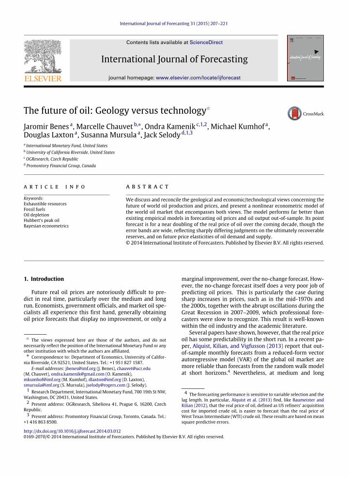
Fig. 1. EIA forecasts of oil production, 2001–2010 (EIA definition ofworldtotal oil supply, in Mbd).
data, about ultimately recoverable oil resources, and aboutthe long-run price elasticities of oil demand and oil supply.
The rest of the paper is organized as follows. Section 2presents various historical forecasts of oil productionmadeby proponents of the technological and geological views.Section 3 presents and discusses the model specificationand parameter estimates. Section 4 contains a detailedanalysis of the estimation results. Section 5 concludes.
2. Historical forecasts of world oil production
The complicated dynamics of world oil supply and oildemand make oil production forecasting very difficult.Fig. 1 shows the track record of the US Energy Informa-tion Administration (EIA). Strikingly, their forecasts exhib-ited an almost continuous decline between 2001 and 2010,with the forecast for 2020 declining by over 20%, or 25mil-lion barrels per day. Earlier EIA forecasts were based on thesimple notion that the supply would be available to satisfyany demand, so these forecasts essentially only consideredthe drivers of demand. This turned out to be far too op-timistic, and more recent forecasts may be reflecting therecognition that physical/geological constraints are start-ing to influence oil production and oil prices.
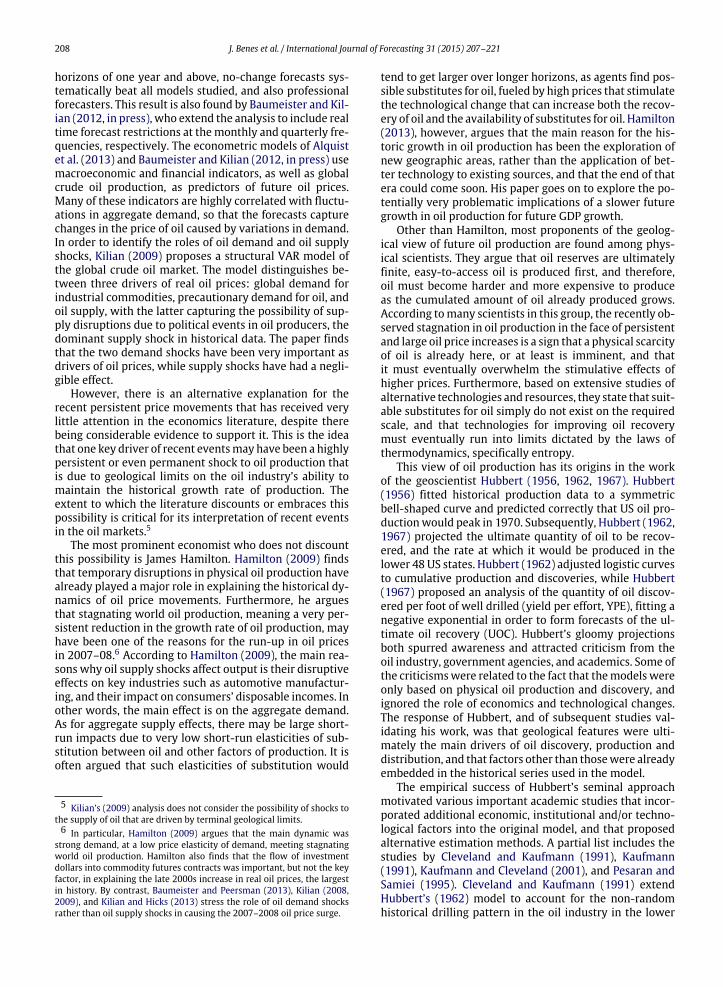
The reason why this may be the case is illustrated inFig. 2, which displays real world oil prices in 2011 US dol-
1994 1996 1998 2000 2002 2004 2006 2008 2010 2012
February 2003 November 2008
Oil Price (average of UK Brent, Dubai, and West Texas)(In U.S. dollars per barrel divided by U.S. CPI; 2011 CPI=1)
0
1
2
3
4
5
6
7
8
February 2003 November 2008
OPEC Spare Capacity (in millions of barrels per day)(Source: EIA)
0
20
40
60
80
100
120
140
0
20
40
60
80
100
120
140
1994 1996 1998 2000 2002 2004 2006 2008 2010 2012
Fig. 2. World US$ oil prices and spare capacity.
lars,12 alongside the OPEC spare capacity inmillions of bar-rels per day (Mbd). Until the end of 2002, spare capacitywas high in historical terms, and this was accompanied byoil prices that had not been growing significantly in realterms. This changed abruptly in early 2003, around thetime of the Iraq war, when spare capacity dropped belowthe 2 Mbd mark, which is considered by many in the in-dustry to be the critical point at which supply becomesa constraining factor. From that moment until the onsetof the Great Recession, real oil prices started a long-termincrease whereby they ultimately more than tripled, be-fore the demand destruction of the Great Recession led toa sudden increase in spare capacity and a steep decline inoil prices. However, this only brought temporary relief tothe demand-supply balance in the oil market, for two rea-sons. First, as we have seen in Fig. 1, oil production neverregained its historical growth rate of 1.5%–2% per annumafter 2005, and, in fact, actually remained on a plateau forseveral years. Second, partial demand recoveries restartedfrom 2009 onwards in many economies. Spare capacitytherefore approached 2 Mbd again, and oil prices ratch-eted up. With the exception of the period of deep reces-sion, the combination of a plateau in actual oil productionand renewed pressure on spare capacity indicates that the
12 The figure is normalized so that the real oil price in 2011 equals 104.This makes the units intuitive, given that the average 2011 nominal oilprice was US$ 104. The same normalization is adopted in all subsequentcharts of the real oil price.
J. Benes et al. / International Journal of Forecasting 31 (2015) 207–221 211
40
45
50
55
60
65
702003 Forecast 2005 Forecast 2010 Forecast
40
45
50
55
60
65
70
2000 2002 2004 2006 2008 2010 2012 2014 2016 2018 2020
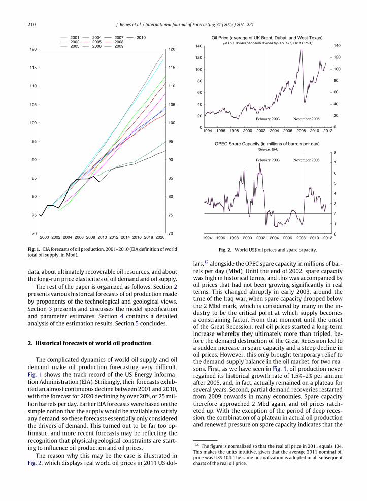
Fig. 3. Colin Campbell’s forecasts for oil production, 2003–2010(Campbell’s definition of regular conventional oil, in Mbd).
physical constraints on oil production started to have anincreasing impact on prices.
Proponents of the geological viewof oil productionhavea track record that can be compared to that of the EIA.Fig. 3 shows the track record of Colin Campbell, a former oilgeologist who has become one of the most influential pro-ponents of the geological view. The one caveat in such acomparison is that different agencies and individuals pro-duce forecasts for different aggregates of oil production.For the EIA, we showed the forecasts for the world’s totaloil supply, which is defined as crude oil plus Natural GasLiquids (NGL) and other liquids, plus refinery processinggains. For Campbell, we show historical forecasts for regu-lar conventional oil. This definition covers over 75% of theworld total oil production; although it is based on EIA data,it excludes heavy oil (<17.5 deg API), bitumen, oil shale,shale oil, deepwater oil and gas (>500 m), polar oil andgas, and NGL from gas plants. Furthermore, the Interna-tional Energy Agency (IEA) uses yet another definition thatis slightly less encompassing than the EIA’s, but more en-compassing than Campbell’s, namely crude oil plus NGL.We will use IEA data in our empirical analysis. We haveused EIA data in Fig. 1 because the EIA produces annualforecasts while the IEA does not. Fig. 3 shows that Camp-bell’s forecasts have also erred, but on the pessimistic sidethis time. The differences from ex-post realized productiondata are somewhat smaller than those for the EIA, whose2001 estimate for 2010 overestimates actual production by
8.7 Mbd, compared to a 2003 underestimate by Campbellof 4.5 Mbd.
Campbell’s methodology is based on an extremely de-tailed knowledge, country by country, of production andexploration data that go back to his participation in theconstruction of an industry database in the early 1990s.Another methodology that is used by proponents of thegeological view is curve fitting for world oil production.13As this approach yields econometrically testable equationsfor the production profile, we will pursue this in detail inthis paper. A particularly tractable specification is knownas Hubbert linearization. This is based on Deffeyes (2005),whodevelops a considerably simplified version of the anal-ysis by Hubbert (1982). We adopt the notation that qtrepresents annual oil production at time t , Qt representscumulative production until time t , and Q̄ represents ulti-mately recoverable reserves, or cumulative production bythe time the last oil well in the world runs dry. Hubbertstates that annual production can be approximated use-fully by the logistic curve
qt = αsQt
Q̄ − Qt
Q̄
. (1)
This is a bell-shaped curve, and it states that, in any givenyear, the actual production is determined by the cumula-tive production that has already taken place, and by thefraction of oil that remains to be produced. The latter dom-inates from exactly the point where half of all oil has beenproduced, Qt = Q̄/2. At that point, annual oil productionpeaks, and subsequent production starts to decline. This lo-gistic function can be transformed by dividing Eq. (1) byQt ,which produces a linear relationship between cumulativeproduction and the ratio of current to cumulative produc-tion:qtQt
= αs −αs
Q̄Qt . (2)
Given that both αs and Q̄ are unknowns for econometricpurposes, this can be written asqtQt
= αs − βQt . (3)
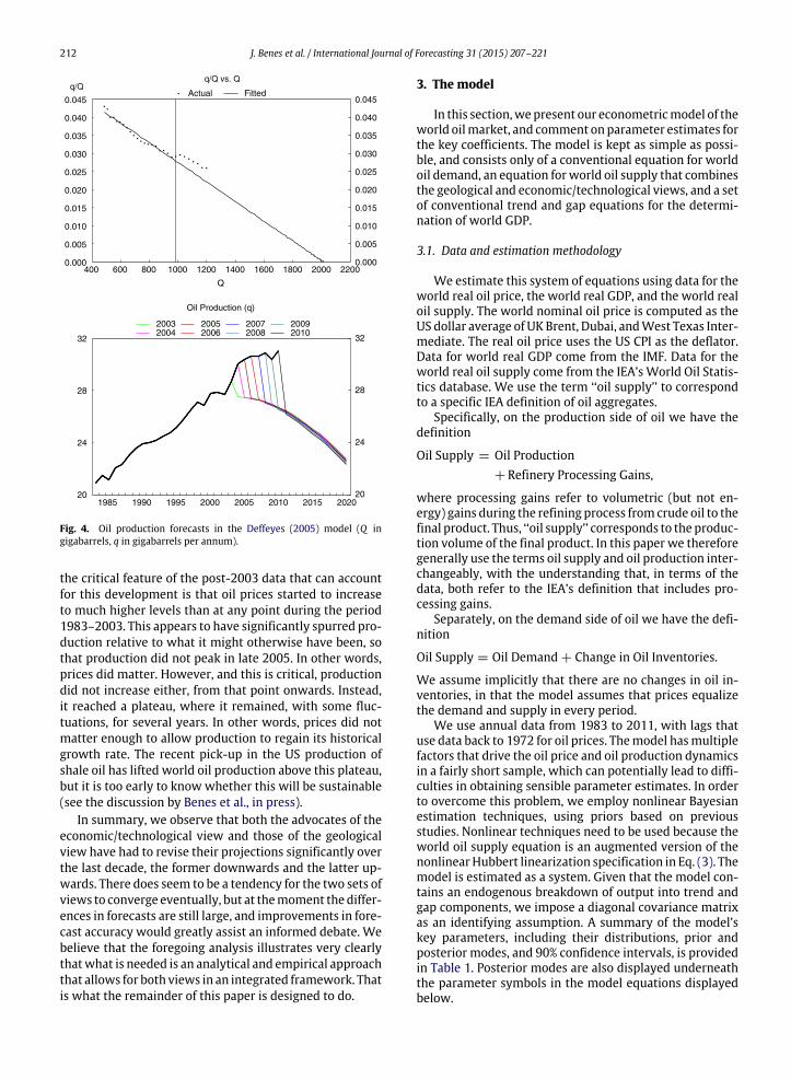
Deffeyes (2005) finds that this relationship fits both USand world data very well until 2003, the last data pointin his 2005 study, with the two series being very closeto a straight line relationship for the period 1983–2003.His fit of the data indicates a logistic curve with a peakin late 2005, and a decline in world oil production there-after. Deffeyes responds to the economic/technologicalview that higher prices should spur additional technolog-ical development, and hence, production that might delaythe peak, by stating that ‘‘improved technologies and in-centives have been appearing all along, and there seems tobe no dramatic improvement that will put an immediatebend in the straight line’’.
As we show in the top half of Fig. 4, this prediction wasnot borne out by subsequent events, as significant posi-tive deviations from Deffeyes’ straight line started to ap-pear immediately after 2003. As we have seen in Fig. 2,
13 See UK Energy Research Centre (2009) for a very detailed discussion.
212 J. Benes et al. / International Journal of Forecasting 31 (2015) 207–221
Actual Fitted
20
24
28
32
20032004
20052006
20072008
20092010
0.000
0.005
0.010
0.015
0.020
0.025
0.030
0.035
0.040
0.045
0.000
0.005
0.010
0.015
0.020
0.025
0.030
0.035
0.040
0.045
600 800 1000 1200 1400 1600 1800 2000
Q
20
24
28
32
1985 1990 1995 2000 2005 2010 2015 2020
Oil Production (q)
400 2200
Fig. 4. Oil production forecasts in the Deffeyes (2005) model (Q ingigabarrels, q in gigabarrels per annum).
the critical feature of the post-2003 data that can accountfor this development is that oil prices started to increaseto much higher levels than at any point during the period1983–2003. This appears to have significantly spurred pro-duction relative to what it might otherwise have been, sothat production did not peak in late 2005. In other words,prices did matter. However, and this is critical, productiondid not increase either, from that point onwards. Instead,it reached a plateau, where it remained, with some fluc-tuations, for several years. In other words, prices did notmatter enough to allow production to regain its historicalgrowth rate. The recent pick-up in the US production ofshale oil has lifted world oil production above this plateau,but it is too early to know whether this will be sustainable(see the discussion by Benes et al., in press).
In summary, we observe that both the advocates of theeconomic/technological view and those of the geologicalview have had to revise their projections significantly overthe last decade, the former downwards and the latter up-wards. There does seem to be a tendency for the two sets ofviews to converge eventually, but at themoment the differ-ences in forecasts are still large, and improvements in fore-cast accuracy would greatly assist an informed debate. Webelieve that the foregoing analysis illustrates very clearlythatwhat is needed is an analytical and empirical approachthat allows for both views in an integrated framework. Thatis what the remainder of this paper is designed to do.
3. The model
In this section,wepresent our econometricmodel of theworld oilmarket, and comment onparameter estimates forthe key coefficients. The model is kept as simple as possi-ble, and consists only of a conventional equation for worldoil demand, an equation forworld oil supply that combinesthe geological and economic/technological views, and a setof conventional trend and gap equations for the determi-nation of world GDP.
3.1. Data and estimation methodology
We estimate this system of equations using data for theworld real oil price, the world real GDP, and the world realoil supply. The world nominal oil price is computed as theUS dollar average of UK Brent, Dubai, andWest Texas Inter-mediate. The real oil price uses the US CPI as the deflator.Data for world real GDP come from the IMF. Data for theworld real oil supply come from the IEA’s World Oil Statis-tics database. We use the term ‘‘oil supply’’ to correspondto a specific IEA definition of oil aggregates.
Specifically, on the production side of oil we have thedefinition
Oil Supply = Oil Production+ Refinery Processing Gains,
where processing gains refer to volumetric (but not en-ergy) gains during the refining process fromcrude oil to thefinal product. Thus, ‘‘oil supply’’ corresponds to the produc-tion volume of the final product. In this paper we thereforegenerally use the terms oil supply and oil production inter-changeably, with the understanding that, in terms of thedata, both refer to the IEA’s definition that includes pro-cessing gains.
Separately, on the demand side of oil we have the defi-nition
Oil Supply = Oil Demand + Change in Oil Inventories.
We assume implicitly that there are no changes in oil in-ventories, in that the model assumes that prices equalizethe demand and supply in every period.
We use annual data from 1983 to 2011, with lags thatuse data back to 1972 for oil prices. Themodel hasmultiplefactors that drive the oil price and oil production dynamicsin a fairly short sample, which can potentially lead to diffi-culties in obtaining sensible parameter estimates. In orderto overcome this problem, we employ nonlinear Bayesianestimation techniques, using priors based on previousstudies. Nonlinear techniques need to be used because theworld oil supply equation is an augmented version of thenonlinearHubbert linearization specification in Eq. (3). Themodel is estimated as a system. Given that the model con-tains an endogenous breakdown of output into trend andgap components, we impose a diagonal covariance matrixas an identifying assumption. A summary of the model’skey parameters, including their distributions, prior andposterior modes, and 90% confidence intervals, is providedin Table 1. Posterior modes are also displayed underneaththe parameter symbols in the model equations displayedbelow.
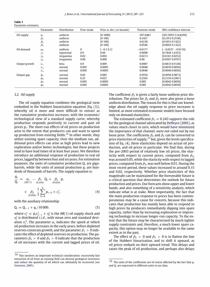
J. Benes et al. / International Journal of Forecasting 31 (2015) 207–221 213
Table 1Parameter estimates.
Parameter Distribution Prior mode Prior st. dev. (or bounds) Posterior mode 90% confidence interval
Oil supply αs uniform [0 1000] 507.6483 [501.9955 514.8299]β1 uniform [0 100] 0.2427 [0.2353 0.2538]β2 uniform [0 100] 0.6238 [0.5053 0.7422]β3 uniform [0 100] 0.0546 [0.0043 0.1322]
Oil demand αd uniform 0 [−0.1 0.1] −0.0177 [−0.0237 −0.0119]γ1 lognormal 0.9 0.09 0.9098 [0.7844 1.0352]γ2 invgamma 0.02 0.002 0.0213 [0.0181 0.0252]γ3 invgamma 0.06 0.006 0.06 [0.0507 0.0707]
Output growth λ1 beta 0.9 0.009 0.8987 [0.8833 0.9128]λ2 normal 0.005 0.0005 0.0048 [0.0039 0.0056]λ3 normal 0.005 0.0005 0.0048 [0.0040 0.0056]
Output gap φ1 normal 0.85 0.085 0.9556 [0.9058 0.9873]φ2 normal 0.25 0.025 0.2565 [0.2156 0.2967]φ3 normal 0.005 0.0005 0.005 [0.0042 0.0058]φ4 normal 0.005 0.0005 0.005 [0.0042 0.0058]
3.2. Oil supply
The oil supply equation combines the geological viewembodied in the Hubbert linearization equation (Eq. (3)),whereby oil is more and more difficult to extract asthe cumulative production increases, with the economic/technological view of a standard supply curve, wherebyproduction responds positively to current and past oilprices pt . The short-run effects of oil prices on productionarise to the extent that producers can and want to speedup production from existing fields.14 In other words, theyutilize existing spare capacity. Over the medium run, ad-ditional price effects can arise as high prices lead to newexploration and/or better technologies, but these projectstend to have lead times of at least four years. We thereforeintroduce an additional response of production to real oilprices, laggedbybetween four and six years. For estimationpurposes, the units of cumulative production Qt are giga-barrels, while the units of annual production qt are hun-dreds of thousands of barrels. The supply equation is:qtQt
= αs(507.7)
− β1(0.243)
Qt + β2(0.624)
pt
+ β3(0.056)
13
6k=4
pt−k + ϵst , (4)
with the auxiliary relationship
Qt = Qt−1 + qt/10 000. (5)
where ϵst = φsϵ
st−1 + ηs
t is the AR(1) oil supply shock andηst is distributed i.i.d., with mean zero and standard devi-
ation σ 2s . The parameter αs indicates the speed at which
oil production increases in the early years, before depletedreserves constrain growth, and the parameter β1 > 0 indi-cates the effect of depleted reserves on production. The pa-rameters β2 > 0 and β3 > 0 indicate that the productionof oil increases with the current and lagged prices of oil.
14 This involves an important technical consideration: excessively fastextraction of oil from an existing field can destroy geological structuresand reduce the quantity of oil which can ultimately be recovered (seeSimmons, 2005).
The coefficient β1 is given a fairly loose uniform prior dis-tribution. The priors for β2 and β3 were also given a looseuniform distribution. The reason for this is that our knowl-edge about the oil supply response to price increases islimited, as most estimated economic models have focusedonly on demand elasticities.
The estimated coefficient β1 = 0.243 supports the rolefor the geological channel advocated by Deffeyes (2005), asvalues much closer to zero, which would have minimizedthe importance of that channel, were not ruled out by ourloose prior. The coefficients β2 and β3 can be converted toprice elasticities of supply,15 but, given the levels specifica-tion of Eq. (4), these elasticities depend on actual oil pro-duction, and oil prices in particular. We find that, duringthe pre-2003 period of relatively low oil prices, the elas-ticity with respect to current prices, computed from β2,was around 0.05,while the elasticitywith respect to laggedprices, computed from β3, was well below 0.01. During themost recent period, these values increased to around 0.15and 0.02, respectively. Whether price elasticities of thismagnitude can be maintained for the foreseeable future isa critical question that determines the outlook for futureproduction and prices. Our forecasts showupper and lowerbands, and also something of a sensitivity analysis, whichindicate what is at stake. Most importantly, the fact thatthe main production response to prices has been contem-poraneous may be a cause for concern, because this indi-cates that production has mainly been able to respond tohigh prices by producers immediately dipping into sparecapacity, rather than by increasing exploration or improv-ing technology to increase longer-run capacity. To the ex-tent that the future may be characterized by much tightersupply constraints and, therefore, a much lower spare ca-pacity, this option may no longer be available to the sameextent as in the past.
The effect of β2 > 0 and β3 > 0 is to flatten the lineof the Hubbert linearization, and to shift it upward, asoil prices embark on their upward trend. This delays andraises the peak of oil production, and perhaps also delays
15 The units of the coefficients are of course affected by the fact that qtand Qt are expressed in different units in our data.
214 J. Benes et al. / International Journal of Forecasting 31 (2015) 207–221
the point at which qt = 0. For example, estimating thecurve with β2 and β3 set to zero, over the period 1983–2003, when oil prices were relatively low and steadyon average, produces estimates that generate a steeplydownward sloping line. Extending the sample period to1983–2010, and allowing for β2 > 0 and β3 > 0 to includedata points with higher oil prices that raise the averageprice of oil over the sample, raises and flattens the curve.However, this does not remove the tendency for oil pro-duction to decline eventually, unless real oil prices were tokeep rising steeply and indefinitely.
3.3. Oil demand
Oil demand is specified according to the standard viewthat a combination of economic activity (GDP) and oilprices drives world oil demand. Higher economic activityincreases the demand for oil, since production requires oilas an input, and higher oil prices reduce the demand foroil by increasing the incentive to find substitutes for oil.The price elasticity is expected to be small in the short run,but it may rise in the long run as substitution takes place.For example, the stock of cars turns over very slowly, overmore than a decade.16 We therefore include both currentoil prices and a 10-year moving average of oil prices in ourexplanatory variables. The demand equation is estimatedin differences. We have
1 ln qt = αd(−0.018)
+ γ1(0.910)
1 ln gdpt − γ2(0.021)
lnpt
pt−1
− γ3(0.06)
ln
pt−1
pt−10
9
+ ϵdt , (6)
where ϵdt = φdϵ
dt−1 +ηd
t is the AR(1) demand shock and ηdt
is distributed i.i.d., withmean zero and standard deviationσ 2d . The prior for γ1 was set to reflect the tight relationship
between GDP and oil demand that has been found in nu-merous previous studies, including a recent analysis in theApril 2011 IMF World Economic Outlook (IMF, 2011). Thedistribution is also set tightly to reflect the robustness ofthis link in the literature. The prior distributions for γ2 andγ3 are also set tightly, reflecting a considerable degree ofconsensus about these values in the literature. The priormodes are set so that the short-run elasticity of demand isless than the long-run elasticity. We also allow for the pos-sibility that γ2 and γ3 may be up to 2.5 times larger at veryhigh oil prices, because such prices would dramatically in-crease the incentives to substitute away from oil.17 Specif-ically, elasticities are unaffected at the average oil pricesseen prior to 2008, rise by roughly a factor of 1.75 at theaverage prices of 2008 and 2011, and eventually rise by afactor of at most 2.5 at themuch higher prices projected bythe model out to 2021.
The estimate for the income elasticity of oil demandγ1 is consistent with other studies, which have found
16 There are grounds for doubt as to whether long-run elasticities cancontinue indefinitely to be much higher than short-run elasticities. Seethe discussion in Section 4.5.17 To keep the exposition simple, this is not shown in Eq. (6).
that, on average, industrialized countries display a lowerincome elasticity around 0.5, reflecting a less oil-intensiveand more service-intensive production structure, whilemany key emerging markets, which have been the maindrivers of recent world economic growth, display incomeelasticities of around 1. The estimated price elasticitiesof demand are in line with the estimates reported bythe IMF (2011), with a very low short-run elasticity of0.02 and a long-run elasticity (after 10 years) of 0.08. Thecombination of low price elasticities of supply and demandimplies that any reduction in the available supply, or evenan inadequate growth of supply relative to past trends,must lead to either much higher oil prices or an economiccontraction, or a combination of the two.
3.4. GDP equations
The feedback fromoil prices to economic activity is cap-tured by the reduced-form specificationgdpt = pot t ∗ yt , (7)where pot t is potential output and yt is the output gap, andwhere oil prices enter into the equations determining bothof these terms, as will be discussed below. Furthermore,this specification allows us to introduce shocks to the out-put gap (transitory shocks to the level of output), potentialoutput (permanent shocks to the level of output), and thepotential output growth (transitory but persistent shocksto the growth rate of output) separately. The richness ofthis specification helps us to model the complicated inter-actions of oil price movements and GDP, where both thetrend and gap decline if oil prices increase. However, thereis not enough variation in the historical data to providewell-determined estimates of these separate effects basedon a single observed variable. One advantage of adoptingBayesian estimation techniques is that we can adopt rea-sonable and tightly set priors that help with the identifica-tion of these three different shocks to output.
3.4.1. Level of potential GDP
Potential GDP is given by
1 ln pot t = ln gt + ϵpott , (8)
where ϵpott is a shock to the level of potential output and
gt is the growth rate of potential output. Oil prices do notenter this equation, since we assume that the dynamiceffects of oil prices on potential output will be captured inthe potential growth rate equation.
3.4.2. Growth rate of potential GDPThe growth rate of potential world GDP is specified as
fluctuating around an exogenous long-run trend, with oilprice changes making the fluctuations more severe. Oilprices are allowed to have persistent but not permanenteffects on the growth rate of GDP. We haveln gt = λ1
(0.899)ln gt−1 + (1 − λ1) g
(0.04)
− λ2(0.005)
1 ln pt − ρ
(0.07)
− λ3
(0.005)
1 ln pt−1 − ρ
(0.07)
+ ϵ
gt , (9)
J. Benes et al. / International Journal of Forecasting 31 (2015) 207–221 215
where ϵgt is a shock to the growth rate of potential output,
g is the average or steady state growth rate of GDP, and ρis the average growth rate of real oil prices. The estimatedsteady state world annual growth rate of potential GDP is4%. The average annual growth rate of real oil prices, whichis the growth in oil prices at which themodel assumes zeroeffects of oil prices on output growth, is 7%. The resultsindicate that an oil price growth rate that is higher than thehistorical average has a small but significant negative effecton the growth rate of potential. Both exogenous shocks ϵ
gt
and oil price fluctuations cause the growth rate to deviatequite persistently from its long-run value, given that theestimated coefficient on the lagged growth rate equals 0.9.
3.4.3. Output gapApart from allowing for an effect of higher oil prices on
the growth rate of potential output, the model also allowsfor the possibility that higher oil prices can cause fluctu-ations in the amount of excess demand in the economy.Specifically, we have
1 ln yt =
φ1
(0.956)−1
ln yt−1 + φ2
(0.257)1 ln yt−1
− φ3(0.005)
1 ln pt − ρ
(0.07)
− φ4
(0.005)
1 ln pt−1 − ρ
(0.07)
+ ϵ
yt , (10)
where ϵyt represents a shock to the level of aggregate de-
mand. Similarly to the equation for potential, the coeffi-cient estimates show that higher oil prices have a small butsignificant negative effect on excess demand, and that thiseffect is highly persistent.
4. Analysis
We now study the estimation results in more detail,by analyzing the implications of the parameter estimatesthat have been discussed for themodel’s impulse responsefunctions, interpretation of history, and forecast accuracy,and for current forecasts of oil production, oil prices andGDP.
4.1. Impulse response functions
Fig. 5 shows the impulse response functions of themodel, with three columns for the responses of oil produc-tion, the real price of oil and GDP, and five rows for thefive shocks, oil supply shocks, oil demand shocks, outputgap shocks, potential growth shocks, and potential levelshocks. All impulse responses are shown in percentage de-viations fromcontrol, after removing any underlying trend.
Oil supply shocks occur separately from, and in additionto, the geological tightening effects of Hubbert’s curve inEq. (4).We find that, relative to oil demand shocks and out-put gap shocks, such shocks have been comparatively smalland transitory in the recent data, and consequently theireffects on real oil prices have been transitory as well, al-though the upward spikes observed in real oil prices when
these shocks did occur have been significant. The top rowof Fig. 5 shows that a negative oil supply shock createsa five year cycle in which output is below potential, andwhere the contraction in GDP is about half as large as thecontraction in oil supply. Due to very low short-run de-mand and supply elasticities, oil prices increase dramati-cally in the short run, bymore than 30 times themagnitudeof the supply contraction, but they subsequently returnquickly to trend.
Oil demand shocks have been significantly larger insize, and have been a major contributor to high oil prices,especially in the period prior to the Great Recession, and inthe recent partial recovery from that recession. Oil demandshocks have also had much more persistent effects on oilproduction and GDP than oil supply shocks. Their effect onthe real price of oil has been less sharp, but again morepersistent.
The main shocks that explain the behavior of oil pricesduring the crisis are output gap shocks, which are illus-trated in the third row of Fig. 5. Estimated output gapshocks have very large and persistent effects on GDP thatlead to similarly large and persistent effects on oil demand.Of course, the dominant output gap shock during the cri-sis has been a negative shock that reduced the economicactivity and oil demand. The resulting large effect on theoil price is a major part of the model’s explanation for thesteep drop in oil prices following the onset of the Great Re-cession.
The impulse responses for potential growth rate shocksare illustrated in the fourth row of Fig. 5. These shocks aresmaller in size than output gap shocks, but they havemuchmore persistent effects on output and oil production. Theireffects on the real price of oil are less dramatic, becausethese shocks only lead to a gradual increase in the oildemand, so that low short-run price elasticities of demandand supply do not play a significant role.
Finally, potential level shocks do not contributemuch tothe overall variability in the model. When they do occur,the effects on output, oil production and oil prices are ofcourse highly persistent.
4.2. Interpretation of history
Fig. 6 shows the estimated shocks of the model. Figs. 7and 8 showmodel decompositions of the post-2002move-ments in oil prices and oil supply into the contributions ofthe three shocks that account for most of the variability inthe model. In each case, the broken line represents the no-shock paths. The solid line in the top left panel correspondsto all shocks in themodel, and is therefore, by construction,identical to the data. The solid lines in the remaining panelsshow the separate contributions of the estimated shocks tooil demand, oil supply, and the output gap.
We begin with Fig. 7, the decomposition of oil prices.The most important observation is that it is not the shocksthat are the major driving force behind the trend increasein oil prices in our model. Rather, the no-shocks scenariopredicts an increase in oil prices that is not far from the ac-tual trend.18 The reason for this is the significant estimate
18 The actual trend does show a positive deviation from the no-shocksscenario. The main factor is unexpectedly strong demand from emergingeconomies post-2002.

216 J. Benes et al. / International Journal of Forecasting 31 (2015) 207–221
Fig. 5. Impulse responses (in percent level deviations from control; shocks in rows, variables in columns).
of the Hubbert linearization coefficient β1 in the oil sup-ply curve. This confirms that the problem of oil becomingharder and harder to produce in sufficient quantities wasan important factor that would have increased oil pricessignificantly, regardless of shocks.
As for the contribution of shocks, by 2008, oil prices hadreached a level that was 60% higher than what the modelwould have predicted on the basis of 2002 information.In the earlier years, the major contributing factors werea very strong oil demand, mainly from booming emerg-ing economies, and a positive world output gap. Oil supplyshocks, at least until some time in 2005, actually helped,ceteris paribus, to keep oil prices lower than they wouldotherwise have been. However, as we have seen, world oilproduction stayed on a plateau from that time onward, andby 2008, an insufficient world oil supply had become themajor factor behind high oil prices. The impact of the fi-nancial crisis in 2008 associated with the Great Recessionwas so severe that, in 2009, oil prices dropped below theoriginal 2002 forecast. The model attributes roughly halfof this drop to a negative output gap shock, and the otherhalf to a positive oil supply shock. The latter is the model’s
interpretation of the increase in oil excess capacity in 2009.By 2011, real oil prices had returned to their 2008 average(not peak) levels. The model attributes almost all of thisto negative oil supply shocks, with oil demand and out-put gap shocks showing nomajor trend reversal after 2008.In other words, the insufficient growth of world oil supplythat had begun to assert itself between 2005 and 2008 re-turned to center stage, as production remainedon the sameapproximate plateau that it had reached in late 2005.
Fig. 8 decomposes oil production, in gigabarrels per an-num.19 We observe that, except for 2009, production wasconsistently and sometimes significantly above the trendpredicted by themodel in 2002.However, oil supply shocksonly made a minor contribution to this development, withthemajor driving forces coming from booming oil demandand, from 2006 to 2008, positive output gaps. Because bothof these shocks lead to higher oil prices, the price mecha-nism that we added to Deffeyes’ (2005) Hubbert lineariza-tion specification is key to being able to account for the
19 As was explained in Section 3.1, this means that it decomposes thedata series ‘‘oil supply’’ from the IEA database.

J. Benes et al. / International Journal of Forecasting 31 (2015) 207–221 217
Oil Supply Shocks
Oil Demand Shocks
1983 1988 1993 1998 2003 2008
Output Gap Shocks
–2
0
2
4
–3
–2
–1
0
1
2
–4
–3
–2
–1
0
1
1983 1988 1993 1998 2003 2008
1983 1988 1993 1998 2003 2008
Fig. 6. Historical residuals (in percentages).
post-2003 deviations from the pure geological explana-tion of oil production and prices. However, it is of coursethis geological explanation that is able to account for thestrong underlying trends in the model, especially the up-ward trend in oil prices.
4.3. Relative forecast performance
Fig. 9 shows our model’s out-of-sample rolling fore-casts, from 2001 to 2011, for oil production, oil prices, andthe growth rate of real GDP. The figure shows only thepoint forecasts; error bands will be discussed in the nextsubsection.
The predicted average annual growth rates of oil pro-duction are well below the historical forecasts of the EIA,but above the forecasts made by proponents of the geo-logical view.We therefore find that ourmodel’s accommo-dation of both the geological and economic/technologicalviews leads to estimation results that provide partial sup-port for both, while rejecting pure versions of either. Thisis not unexpected, given our discussion of recent trends inoil production (on a plateau until recently) and spare ca-pacity on the one hand, and of the clear effects of prices inoverturning the pure Deffeyes (2005) model.
However, the projected positive trend in oil produc-tion comes at a steep cost, because the model finds thatit requires a large increase in the real price of oil, whichwould have to nearly double over the coming decade in or-der to maintain an expansion of production that is modestin historical terms. Such prices would far exceed even thehighest prices seen in 2008, which, according to Hamilton(2009), may have played an important role in driving theworld economy into a deep recession.
2005 2008 2005 2008
2005 2008 2005 2008
40
60
80
100
120
40
60
80
100
120
40
60
80
100
120
40
60
80
100
120
2002 2011
All Shocks
2002 2011
Oil Demand Shocks
2002 2011
Oil Supply Shocks
2002 2011
Output Gap Shocks
Fig. 7. Contributions of different shocks to oil prices (in real 2011 USdollars).
28
29
30
31
32
2005 2008
28
29
30
31
32
2005 2008
28
29
30
31
32
28
29
30
31
32
2002 2005 2008 2011 2002 2005 2008 2011
All Shocks Oil Demand Shocks
2002 2011
Oil Supply Shocks
2002 2011
Output Gap Shocks
Fig. 8. Contributions of different shocks to oil production (in gigabarrelsper annum).
This negative effect of higher oil prices on the GDP ispresent in themodel’s forecasts for GDP growth, but, as wewill see, it ismodest. This raises the question ofwhether fu-ture versions of the model should include nonlinearities inthe output responsewhich are similar to the nonlinearitiesin our oil demand equation. There is likely to be a critical

218 J. Benes et al. / International Journal of Forecasting 31 (2015) 207–221
1995 2000 2005 2010 2015
1990 1995 2000 2005 2010 2015 2020
1990 1995 2000 2005 2010 2015 2020
24
26
28
30
32
34
50
100
150
0
2
4
Oil Production
Real Price of Oil
GDP Growth Rate
1990 2020
Fig. 9. Out-of-sample rolling forecasts, 2001–2011. (Oil production:gigabarrels per annum; real price of oil: real 2011 US dollars; GDP growthrate: percentage points. Each line starts in the year inwhich the respectiveforecast is made.)
range of oil prices at which the GDP effects of any furtherincreases become much larger than at lower levels, if onlybecause they start to threaten the viability of entire indus-tries such as airlines and long-distance tourism. If this iscorrect, the effect of real oil prices on GDP should be mod-eled as convex. There is support for this conjecture amongoil experts. For example, the chief economist of the Inter-national Energy Agency, Fatih Birol, has repeatedlywarnedthat oil prices have reached a point that could push theworld economy back into recession.20 We will study thispossibility quantitatively in future work.
Fig. 9 shows that our model predicts neither a mean-reverting oil price, like most empirical models of the oilmarket, nor even a random walk, which has been shownto outperform suchmodels in many studies. Rather, it pre-dicts a clear upward trend, which is exactly what we havebeen observing in the data, with the exception of the de-mand destruction of the Great Recession. Furthermore, ourmodel’s out-of-sample predictions for oil production in theearly 2000s are far more accurate than either the contem-poraneous EIA forecasts or the forecasts using either Def-feyes’ or Campbell’s methods. In order to formalize thesecomparisons of forecast accuracies, Table 2 shows the rootmean square errors (RMSEs) of our model’s rolling fore-casts over the period 2003–2011, and compares the fore-casts for the level of oil production to the EIA’s forecasts,the forecasts for the level of oil prices to a random walk,and the forecasts for the level of world GDP to those ofcontemporaneous editions of the IMF’s World Economic
20 See the IEA website at http://www.worldenergyoutlook.org/quotes.asp for a collection of Birol’s recent quotes on this subject.
Table 2Root mean square errors—comparisons (based on out-of-sample rollingforecasts, 2003–2011).
Horizon Real price of oil Oil production GDP levelModel Random
walkModel EIA Model WEO
1 year 14.7 27.7 1.69 1.59 1.82 1.832 years 17.6 47.4 1.97 2.57 3.03 3.413 years 19.9 57.9 2.31 3.51 3.62 4.694 years 22.4 79.0 2.41 4.66 3.74 5.555 years 25.1 100.0 2.69 5.72 3.05 5.00
Point forecast90 pct interval70 pct interval50 pct intervalTighter Oil Supply
28
29
30
31
32
33
34
35
36
37
2000 2002 2004 2006 2008 2010 2012 2014 2016 2018 2020
Fig. 10. Oil output forecast with error bands (in gigabarrels per annum).
Outlook (WEO). For production, our RMSEs are lower thanthose of the EIA’s historical forecasts at all but the one-yearhorizon, and less than half as large at longer horizons. Forprices, the gains from using our model are even larger, es-pecially at longer horizons. For example, at the five-yearhorizon, our model’s RMSE is about a quarter of the RMSEof a random walk. Against the background of the existingliterature, these results are dramatic. The gains are less dra-matic for GDP, but are very substantial nevertheless.21
4.4. Current forecasts
Figs. 10–12 show the model’s current projections, forthe decade from2012 to 2021, for oil production, oil prices,and GDP. The figures contain point forecasts, with errorbands around the forecasts. They also show an alternativescenario that assumes a tighter future oil supply due to alower future elasticity of the oil supplywith respect to con-temporaneous oil prices.Wewill comment on this scenarioat the end of this subsection.
21 We will not emphasize the RMSE differences for GDP further in thispaper, partly because this result may have less to do with our modelingof the oil sector and more with our modeling of the different componentprocesses of output.

J. Benes et al. / International Journal of Forecasting 31 (2015) 207–221 219
Point forecast
90 pct interval
70 pct interval
50 pct interval
Tighter Oil Supply
40
60
80
100
120
140
160
180
200
220
240
2000 2002 2004 2006 2008 2010 2012 2014 2016 2018 2020
Fig. 11. Oil price forecast with error bands (in real 2011 US dollars).
Point forecast90 pct interval70 pct interval50 pct intervalTighter Oil Supply
0.7
0.8
0.9
1.0
1.1
1.2
1.3
1.4
2000 2002 2004 2006 2008 2010 2012 2014 2016 2018 2020
Fig. 12. World GDP (in logs) forecastwith error bands (normalized index,with the log of 2011 world real GDP equal to 1).
Fig. 10 shows oil production, in gigabarrels per annum.The point forecast is for a mean annual growth rate of oilsupply of around 0.9% over the coming decade, which ispositive but well below its historical growth rate of around1.5%–2.0%. The 90% confidence interval is very wide, andreflects high levels of uncertainty concerning the ulti-mately recoverable resources (implicit inβ1), aswell as thesupply anddemand elasticitieswith respect to the oil price.The lower 90% band indicates flat oil production for theentire decade, while the upper band indicates annual pro-duction growth rates that are almost as large as historicalones. It is important to observe that, while the point fore-cast is for an annual growth rate which is approximately as
large as the most recent EIA forecasts, the forecast for theoil price that is behind this production forecast is far higherthan that anticipated by the EIA.
This is seen in Fig. 11, which shows a point forecast thatimplies a near doubling of real oil prices over the comingdecade, and an increase in prices over and above the veryhigh recent levels even under a very optimistic scenario,at the lower 90% confidence interval. The world economyhas never experienced oil prices this high for anything butshort, transitory periods, and we reiterate our previousstatement that this might take us into uncharted territory,where a nonlinear, convex effect of oil prices on outputmight be a more prudent assumption.
Fig. 12 shows forecasts for GDP, with the 2011 worldreal GDP normalized to one. The point forecast is for aroughly 4% per annum real GDP growth rate. The errorbands may appear narrow relative to those for oil pricesand oil production. Nevertheless, the 90% confidence in-terval contains average growth rates as low as 3% per an-num, and as high as 5% per annum. In otherwords, formorepessimistic coefficient values of ultimately recoverable re-sources and elasticities, average world growth would beone percentage point lower.
Finally, Figs. 10–12 also report the point forecast foran alternative scenario where β2 takes a lower value,corresponding to its lower 90% confidence band. Thebaseline value for β2 was estimated over a period when,at most times, it was possible for producers to respond tohigh prices by immediately utilizing ample spare capacity,an option that may not be available to the same extentin a future of tighter supply constraints. We find that thelower value forβ2 has very large effects on the results, eventhough β2 only drops fairly modestly, from 0.624 to 0.505.The average growth rate of oil production drops from 0.9%to 0.5% per annum, the oil price now fully doubles by 2021,and the path for GDP is approximately equal to the lower90% confidence band. This last result implies that this onechange alone reduces the point forecast for average worldGDP growth by around one percentage point.
4.5. Oil and output—open questions
Our data and analysis suggest that there is at least a pos-sibility that wemay be at a turning point for world oil pro-duction and prices. A key concern going forward is that therelationship between higher oil prices and GDP may be-come nonlinear if oil prices become sufficiently high. Theproblem with this is that, at this moment, our historicaldata contain very little information about what that re-lationship might look like. However, we are not entirelywithout information, since a number of authors in othersciences have started to ask pertinent questions, and havedone some early pioneering work.22
There are two key questions under the maintained hy-pothesis of much a lower growth in oil production. First,what is the importance of the availability of oil inputs forcontinued overall GDP growth? Second, what is the substi-tutability between oil and other factors of production?Weemphasize that these concerns focus not on the demandside, but rather on the supply side effects that could resultfrom a stagnating or declining world oil production rate.
22 See Kumhof and Muir (in press) for a more comprehensive overviewand analysis.
220 J. Benes et al. / International Journal of Forecasting 31 (2015) 207–221
As for the contribution of oil to GDP, the main problemis that conventional production functions imply an equal-ity of cost shares and output contributions of oil, whichfor a long time has led economists to conclude that, givenits historically low cost share of around 3.5% for the USeconomy,23 oil can never account for amassive output con-traction, evenwith low elasticities of substitution betweenoil and other factors of production. This view has beenchallenged in several recent articles and books by naturalscientists, who state that it need not hold with a moreappropriate modeling of the aggregate technology. Thesecontributions include those of Ayres and Warr (2005,2010), Hall and Klitgaard (2012), Kümmel (2011), andKümmel, Henn, and Lindenberger (2002), who propose ag-gregate production functions that are based on conceptsfrom engineering and thermodynamics. Several of thesecontributions estimate their own production functions.The estimations are based on technologies that use energy,rather than just oil, but, given the very limited substi-tutability between oil and other forms of energy, this nev-ertheless offers important insights.24 These authors findoutput contributions of energy of up to around 50%, despitethe low cost share of energy. Clearly, if this can be con-firmed in further rigorous econometric studies, the impli-cations forGDPof a lower growth in oil production could bevery large. This view is explored in oil shock simulations inthe IMF’s April 2011World Economic Outlook (IMF, 2011),using the IMF’smulti-regional Dynamic Stochastic GeneralEquilibrium model, the Global Integrated Monetary andFiscal model (GIMF), assuming a technology where oil’soutput contribution far exceeds its cost share. The simula-tions find that, following permanent declines in the growthrate of world oil production, the model generates muchlarger negative output effects than the conventional neo-classical model, because a share of the stock of technologywould become obsolete.25 This channel has never yet beenof sufficient importance to explain the historical data, andour empirical model therefore does not contain it. Chang-ing this would lead to simulation results with lower GDPgrowth levels.
The other key future concern concerns elasticities ofsubstitution. Several important contributions have chal-lenged economists’ automatic assumption that the elas-ticities of substitution between oil and other factors ofproduction must be much higher in the long run than inthe short run. The objections include the fact that this as-sumption is not consistent with the historical facts (Smil,2010),26 real-world practical limits (Ayres, 2007), or thelaws of thermodynamics, specifically entropy (Reynolds,
23 See http://www.eia.gov/oiaf/economy/energy_price.html.24 For the US economy, the historical cost share of total energy has beenaround 7%.25 See e.g. Atkeson and Kehoe (1999) and Kim and Loungani (1992).26 This book describes the major energy transitions in world history,from biomass to coal, oil and nuclear energy. The critical observationis that all these transitions took many decades to complete, were enor-mously expensive, and, crucially, happened at times when a new majorenergy resource of sufficient scale had already been identified clearly.The latter is clearly not the case today, as renewables are not even nearlyof sufficient scale.
2002, Chapter 10). Our empirical model currently makesthe conventional assumption that, after some time, elas-ticities will be higher at higher prices. A plausible alter-native that could reconcile the economists’ view with theabove objections is to assume that elasticities are very lowin the short run (due to rigidities, adjustment costs, etc.),significantly higher in themedium run (as the rigidities areovercome), but much lower again in the long run if thereis a sufficiently large shock to the growth rate of the worldoil supply, because there is a finite limit to the extent thatmachines (and labor) can substitute for energy. If we wereto incorporate this assumption, the model would forecastsignificantly higher oil prices in the event of a sufficientlylarge and persistent shock to world oil supply.
5. Conclusion
The main objective of this paper has been to propose amodel of theworld oilmarket that does not take an a-prioriview of the relative importance of resource constraintsand the price mechanism, and to evaluate it empirically.We do not want to rule out either of these mechanisms,because the recent data indicate convincingly that bothmust have been important. Our empirical representationof this view models oil supply as a combination of theHubbert linearization specification of Deffeyes (2005) anda price mechanism whereby higher oil prices increase theoil production.
Our empirical results vindicate this choice. Our modelperforms far better than competing models in predictingeither oil production or oil prices out-of-sample, in a fieldwhere predictability has historically been low. Our empir-ical results also indicate that, if the model’s predictionscontinue to be as accurate as they have been over the lastdecade, the future will not be easy. While our model is notas pessimistic as the pure geological view, which typicallyholds that binding resource constraints will lead world oilproduction into an inexorable downward trend in the verynear future, our prediction of small further increases inworld oil production comes at the expense of a permanentnear-doubling of real oil prices over the coming decade.This is uncharted territory for the world economy, whichhas never experienced such prices for more than a fewmonths. Our current model of the effect of such prices onthe GDP is based on historical data, and indicates percepti-ble but small and transitory output effects. However, wesuspect that there must be a pain barrier, a level of oilprices above which the effects on GDPwill become nonlin-ear, convex.We also suspect that the assumption that tech-nology is independent of the availability of fossil fuels maybe inappropriate, so that a lack of availability of oilmay alsohave aspects of a negative technology shock. In that casethemacroeconomic effects of binding resource constraintscould be much larger and more persistent, and would ex-tend well beyond the oil sector. Studying these issues ingreater depth will be a priority in our future research.
Acknowledgments
The authors thank the referees and Fred Joutz fortheir comments and suggestions for improvements. SerhatSolmaz and Kadir Tanyeri provided excellent researchassistance.
J. Benes et al. / International Journal of Forecasting 31 (2015) 207–221 221
References
Alquist, R., Kilian, L., & Vigfusson, R. (2013). Forecasting the price ofoil. In G. Elliott, & A. Timmermann (Eds.), Handbook of economicforecasting, Vol. 2 (pp. 427–507). Amsterdam: North-Holland.
Atkeson, A., & Kehoe, P. J. (1999). Models of energy use: putty-puttyversus putty-clay. American Economic Review, 89(4), 1028–1043.
Ayres, R. (2007). On the practical limits to substitution. EcologicalEconomics, 61, 115–128.
Ayres, R., & Warr, B. (2005). Accounting for growth: the role of physicalwork. Structural Change and Economic Dynamics, 16, 181–209.
Ayres, R., & Warr, B. (2010). The economic growth engine—how energy andwork drive material prosperity. Edward Elgar Publishing.
Baumeister, C., & Kilian, L. (2012). Real-time forecasts of the real price ofoil. Journal of Business and Economic Statistics, 30(2), 326–336.
Baumeister, C., & Kilian, L. (in press) What central bankers need to knowabout forecasting oil prices. International Economic Review.
Baumeister, C., & Peersman, G. (2013). The role of time-varying priceelasticities in accounting for volatility changes in the crude oilmarket. Journal of Applied Econometrics, 28(7), 1087–1109.
Benes, J., Kumhof, M., Laxton, D., Maih, J., Solmaz, S., & Zhang, F. (2014).The future of oil: mind the gap. IMF working papers (in press).
Cleveland, C., & Kaufmann, R. K. (1991). Forecasting ultimate oil recoveryand its rate of production: incorporating economic forces into themodels of M. King Hubbert. Energy Journal, 12(2), 17–46.
Deffeyes, K. (2005). Beyond oil: the view from Hubbert’s peak. Hill andWang.
Government Accountability Office (2007). Crude oil: uncertainty aboutfuture oil supply makes it important to develop a strategy for addressinga peak and decline in world oil production. Report to congressionalrequesters.
Hall, C. A. S., & Klitgaard, K. A. (2012). Energy and the wealth of nations:understanding the biophysical economy. Springer-Verlag.
Hamilton, J. (2009). Causes and consequences of the oil shock of 2007–08.Brookings papers on economic activity (pp. 215–261).
Hamilton, J. (2013). Oil prices, exhaustible resources, and economicgrowth. In R. Fouquet (Ed.), Handbook of energy and climate change.Edward Elgar Publishing.
Hirsch, R., Bezdek, R., & Wendling, R. (2005). Peaking of world oilproduction: impacts, mitigation and risk management. United StatesDepartment of Energy.
Hirsch, R., Bezdek, R., & Wendling, R. (2010). The impending world energymess. Apogee Prime.
Hubbert, M. K. (1956). Nuclear energy and the fossil fuels. In: Amer-ican Petroleum Institute Drilling and Production Practice Proceedings(pp. 5–75).
Hubbert, M. K. (1962). Energy resources. Washington, DC: NationalResearch Council, National Academy of Sciences, 1000-D.
Hubbert, M. K. (1967). Degree of advancement of petroleum explorationin United States. American Association of Petroleum Geologists Bulletin,51, 2207–2227.
Hubbert, M. K. (1982). Techniques of prediction as applied to the pro-duction of oil and gas. In S. I. Gass (Ed.), Special publication: Vol. 631.Oil and gas supply modeling (pp. 16–141). Washington: National Bu-reau of Standards.
IMF (2011). Oil scarcity, growth and global imbalances. InWorld economicoutlook (Chapter 3) International Monetary Fund.
Kaufmann, R. K. (1991). Oil production in the lower 48 states: reconcilingcurve fitting and econometric models. Resources and Energy, 13,111–127.
Kaufmann, R. K., & Cleveland, C. J. (2001). Oil production in the lower 48states: economic, geological and institutional determinants. EnergyJournal, 22(1), 27–49.
Kilian, L. (2008). The economic effects of energy price shocks. Journal ofEconomic Literature, 46(4), 871–909.
Kilian, L. (2009). Not all oil price shocks are alike: disentangling demandand supply shocks in the crude oilmarket. American Economic Review,99(3), 1053–1069.
Kilian, L., & Hicks, B. (2013). Did unexpectedly strong economic growthcause the oil price shock of 2003–2008? Journal of Forecasting , 32(5),385–394.
Kim, I.-M., & Loungani, P. (1992). The role of energy in real business cyclemodels. Journal of Monetary Economics, 29(2), 173–189.
Kümmel, R. (2011). The second law of economics—energy, entropy, and theorigins of wealth. Springer-Verlag.
Kümmel, R., Henn, J., & Lindenberger, D. (2002). Capital, labor, energyand creativity: modeling innovation diffusion. Structural Change andEconomic Dynamics, 13, 415–433.
Kumhof, M., &Muir, D. (2014). Oil and theworld economy: some possiblefutures. Philosophical Transactions of the Royal Society A, 372 (in press).
Pesaran, M. H., & Samiei, H. (1995). Forecasting ultimate resourcerecovery. International Journal of Forecasting , 11(4), 543–555.
Reynolds, D. (2002). Scarcity and growth considering oil and energy: analternative neo-classical view. Edwin Mellen Press.
Simmons, M. (2005). Twilight in the desert: the coming Saudi oil shock andthe world economy. Hoboken, New Jersey: John Wiley & Sons.
Smil, V. (2010). Energy transitions—history, requirements, prospects.Praeger.
Sorrell, S., Miller, R., Bentley, R., & Speirs, J. (2010). Oil futures: acomparison of global supply forecasts. Energy Policy, 38, 4990–5003.
UK Energy Research Centre (2009). Global oil depletion—an assessmentof the evidence for a near-term peak in global oil production.
United States Joint Forces Command (2010). The joint operatingenvironment 2010.