a model for equipment replacement due to …webuser.bus.umich.edu/whopp/reprints/a model...

European Journal of Operational Research 63 (1992) 207-221 207 North-Holland

A model for equipment replacement due to technological obsolescence *

Suresh K. Nair

Department of Operations and Information Management, School of Business, U41-IM, University of Connecticut, Storrs, CT 06269-0241, USA

W a l l a c e J. H o p p

Department of Industrial Engineering and Management Sciences, Northwestern University, Evanston, IL 60208, USA

Received June 1990; revised January 1992

Abstract: We consider the problem of deciding whether to keep a piece of equipment or to replace it with a more advanced technology. This decision must take into account both the nature of the available replacement technology and the possibility of future technological advances. Existing models are restrictive in the way they model the appearance of future technologies and the costs and revenues associated with those technologies. In an earlier paper we allowed the probability of appearance of new technologies to be non-stationary in time but required the costs and revenues of technologies to be different but constant over time. In this paper, we allow the technology forecasts and revenue functions associated with technologies to be non-stationary in time and consider salvage values for technologies. We develop a simple and efficient algorithm for finding the optimal decision using a forecast horizon approach. This approach finds the optimal decision in any period with minimal reliance on forecast data.

Keywords: Equipment; innovation; investment; Markov decision; Dynamic Programming

1. Introduction

The replacement of productive equipment ranks among the most important strategic decisions faced by both manufacturing and service firms. This is because purchase of a new piece of equipment often involves a significant cost and can affect the productivity and competitiveness of the firm for several years into the future. In recent years, the difficulty of this problem has been compounded by the fact that technologies are rapidly changing, and what may appear to be a good equipment purchase can soon become obsolete. Under these circumstances, the driving motivation behind replacement decisions is likely to be technological obsolescence, rather than physical deterioration, of the existing equipment. This situation is typical of microcomputers, computerized numerically controlled machines, and other electronics technologies.

Much work has been done in the area of equipment replacement. For a detailed exposition, see the survey in Pierskalla and Voelker (1976).

The traditional approach to the equipment replacement problem emphasizes the physical deterioration of the existing equipment. The basic idea is to replace the equipment when the cost of operating and maintaining it become sufficiently high, in net expected present value terms, to justify a replacement.

Correspondence to:S.K. Nair, Department of Operations and Information Management, School of Business, U41-1M, University of Connecticut, Storrs, CT 06269-0241, USA.

* This work was supported in part by the National Science Foundation under Grant No. ECS-8619732.

0377-2217/92/$05.00 © 1992 - Elsevier Science Publishers B.V. All rights reserved

208 S.K~ Nair, W.J. Hopp / Equipment replacement due to obsolescence

In most traditional models, technology is assumed to remain constant over time. These include Derman (1963) and Hatoyama (1984). This approach would lead to inappropriate decisions if technology does change, as is becoming increasingly common. For example, if technology is changing it may be better to keep the current equipment for a few more years and then take advantage of an improved technology that appears on the market than to replace the current equipment with what is available in the market at the present time. Typically, if the capital costs for purchasing the new equipment are not recouped by the time another advanced technology appears, it would be extremely difficult for decision makers to justify another replacement when the advanced technology appears.

There are a few models that do consider technological change. Traditionally improvements in technology are measured either in terms of increased revenue associated with the new technology or decreased costs of procurement and operation of the new technology. Most of these models assume that technology improves in a deterministic manner, that is, the extent (in terms of costs and revenues) and timing of the technological improvements is known beforehand (Sethi and Chand, 1979). Though assuming that technology improves in a deterministic manner is a good first approximation, these models do not accommodate the reality that technological improvements can rarely be forecasted with certainty.

Only recently have researchers started to model the equipment replacement problem due to technological change under uncertainty. Goldstein, Ladany and Mehrez (1986, 1988) introduce uncertainty using stationary forecasts (that is, forecasts that are constant over time). Hopp and Nair (1991) developed a model using non-stationary technology forecasts but where the revenue generated by various technologies is different but constant over time.

The models incorporating non-stationary technological forecasts use a forecast horizon procedure to find the optimal keep/replace decision. The forecast horizon is the minimum number of periods of forecasted information required to guarantee that the initial decision is optimal, regardless of forecasts in later periods. The reason forecast horizons are important is that it not only reduces the computation and forecasting necessary to arrive at an optimal decision, but also because it ensures that the optimal decision would be no different if data for additional periods were forecasted.

A forecast horizon procedure attempts to identify the forecast horizon as efficiently as possible. If a forecast horizon exists in a particular problem and can be found, then one needs to solve the problem only to that time horizon to compute the optimal decision in the initial period corresponding to any time horizon beyond it, and in particular the infinite horizon. Since the first decision is the only one that the decision maker is committed to make immediately, this approach is well-suited to the equipment replacement problem. The process can be repeated in the next period. We are interested in the infinite horizon here because it is usually not clear what time horizon a firm should consider, and what the status of the firm would be at the end of that time horizon. Using a forecast horizon obviates the need for using an arbitrary time horizon.

Forecast horizon techniques have been used in the context of a variety of applications (for a survey see Bhaskaran and Sethi, 1987) including equipment replacement (Chand and Sethi, 1982). More recently, conditions for the existence of forecast horizons for deterministic (Bean and Smith, 1984) and stochastic (Hopp, Bean and Smith, 1987; Bbs and Sethi, 1988) problems have been developed.

If a forecast horizon does exist, it could be put to use only if it is identified. Algorithms for identifying forecast horizons in general deterministic (Chand and Morton, 1986) and stochastic optimization (Hopp, 1987; B~s and Sethi, 1988) problem are typically cumbersome or inefficient (i.e., they identify forecast horizons that are much longer than necessary). By exploiting the specific structure of the equipment replacement problem we can greatly improve the efficiency of identifying forecast horizons (see Nair, 1988). This paper is an extension of Hopp and Nair (1991) to the equipment replacement case where not only are the technological forecasts non-stationary in time, but also the revenue and cost functions are non-stationary in time. In addition, salvage values have been considered in the present paper. Structural results on the sensitivity of the optimal decision to changes in forecast are also discussed.

S.K. Nair, W.J. Hopp / Equipment replacement due to obsolescence 209

2. Problem formulation

We consider the problem of a firm trying to decide whether to keep a piece of equipment it currently owns or to replace it with a better technology that is currently available on the market. The problem is complicated by the fact that further improvements of technology could occur in the future and these improvements may have a bearing on the current decision. For example, it may be optimal to wait for a few years and take advantage of a better technology when it becomes available. However, whether or when the advanced technology will appear and what its revenue generating potential will be are uncertain. We assume that the firm's objective is to maximize expected discounted present revenue over the infinite horizon.

We model this problem as an infinite horizon non-stationary Markov decision process (MDP). We choose an infinite horizon as it would be better than assuming an arbitrary finite horizon and then making assumptions on the state of the firm at the end of that horizon. The model considered here is restricted to the case of three technologies, viz., the technology on hand, a 'bet ter ' technology currently available on the market, and an 'even better ' technology that may become available in the future. Our notation and approach are described below.

2.1. Notation

We denote the technology currently in use by index 0, the better technology available on the market by index 1, and exactly one advanced technology that may appear in the future by index 2.

We define a 'state' at some point in time, t, by (i, l) where i represents the index of the technology in use by the firm and l the index of the latest technology available on the market. By our definition of the problem, at the beginning of the problem, the state is (0, 1) and the time period is t = 0. Let K i represent the action 'keep technology i' and R~ ( j_<l) represent the action 'replace the current technology with technology j ' in state (i, l).

To formulate a Markov decision process, we suppose the firm can make keep-replace decisions at the beginning of each period. We let rz, represent the (expected) one period revenue generated by technology i in period t, cit represent the expected capital cost of purchasing technology i in period t, and sit represent the salvage value received from selling technology i in period t. We assume ri,, ci, and sit are bounded. Notice that the revenue, cost and salvage value functions are only time dependent and not age dependent. This would be reasonable for classes of equipment not subject to physical deterioration, like microcomputers and controls, etc.

Let Pt be the probability of appearance of technology 2 in period t given that it has not appeared in period t - 1 or earlier. Note here that though the cost and revenue functions may vary over time, their values are essentially known (or can be estimated). However, the period of appearance of the new technology is uncertain. Again, this kind of situation is appropriate for advanced technology wherein the technical parameters and specifications of the new technology may be decided on beforehand, and the appearance of technology on the market would depend on breakthroughs achieved, market conditions, etc.

Let /3 be the one period discount factor (where /3 < 1) and f ,r( i , l) represent the maximal expected discounted return of being in state (i, l) in period t, if an optimal policy is followed from periods t through some time horizon T (T>_ t). The 'boundary condition', i.e., when t = T, is represented as L(i , l ) - f [ ( i , 1).

2.2. Approach

To find the optimal decision in any state, we need to calculate the value function ftT(i, I). Further, we would like to solve the problem for an infinite horizon, i.e., when T = oo. However, since that would entail making infinite calculations, we will first solve the problem for some finite T, and then extend

210 S.K. Nair, W..Z Hopp / Equipment replacement due to obsolescence

these results to the infinite horizon case using forecast horizon techniques. We start by first stating the following dynamic programming recursive equations describing the problem:

R1 : _ C l t + s o t + r l t _ k / 3 { ( 1 r 1 --Pt+l)f t+l( , 1) +pt+l f tTl (1 , 2)}, f t r (0 , 1) = max (1)

T 0 r 0 K0: rot +/3{(1 - P t + l ) f t + , ( , 1) +Pt+,L+I( , 2)}.

The above expression states that in state (0, 1) in period t, there are only two actions possible, either 'replace with technology 1' (represented by R 1) or 'keep technology 0' (represented by K0). In the former case, a cost of cl, is incurred in purchase of technology 1, a salvage value of So, is collected by selling technology 0, and a one period revenue of rl, accrues from the technology purchased. In addition, a discounted future stream of revenue accrues which depends on whether the new technology 2 does not appear (in which case the state in the next period will be (1, 1)), or appears (in which case the state in the next period will be (1, 2)). If K 0 is the action chosen, then a revenue of rot is collected in addition to the discounted future stream of revenue. This future stream would again depend on whether the new technology 2 does not appear (in which case the state will be (0, 1)) or it appears (the state would be (0, 2)).

Since in state (1, 1) the only decision available is to 'keep technology 1', (it can be proved using Lemma l(a) presented later that it would never be optimal to go back to technology 0, once technology 1 is purchased) the functional equation in this case would be

r 1 p r f tT(l , 1) = r l t 4-/3{(1 --Pt+l)ft+l( , 1) + t+lft+l(l , 2)}. (2)

The functional equations for the other possible states are given by the following expressions using the same reasoning as explained above:

R2: - -C2 t+SOt+r2 t+/3 f tT+l (2 , 2),

r 0 r 1 f , ( , 2 ) = m a x g l : -C l t+so t - l - r l t+ /3 f t + l ( , 2 ) , (3)

~Ko: ro,+/3Lr~(O, 2),

[R2: --C2t + Slt + r2t + /3 f tT l (2 , 2 ) , f , r (1 , 2) = max r 1 , (4)

K,: rlt -1-/3ft + 1( , 2)

r 2 r 2 = q-/3L+l( , 2). (5) f, ( , 2) r2t

The above expressions are valid for t = 0 . . . . . T - 1. For the backward recursion of dynamic programming to work, we need to define the functional value of each state when t = T. These are called the boundary conditions and we are representing it by L(i, l). As long as T is finite, these actions can be computed using backward recursion. In the usual T period problem, we take L(i, l ) = 0 for all i, l. However, as we shall see later, using alternate values of L(i, l) can give useful results.

We let 7rtr(i, l) represent the action, i.e., either K i or Rj ( l > j >i) , that achieves the above maximizations (i.e., rrtT(i, l) is the optimal action in state (i, I) in period t of the T period problem).

The results of Hopp, Bean and Smith (1987) show that, since /3 < 1 and rit, cit , and sit are bounded, f f ( i , l) converges to a limiting value function ft(i, l) as T --+ oo (henceforth, we will drop the superscript T to represent the infinite horizon case). Furthermore, since the set of actions in state (i, l) is finite, their results imply that if the infinite horizon optimal decision, written rrt(i, l), is unique (i.e., the revenue streams from alternative actions is not exactly equal), then there exists a finite horizon r such that 7rf(i, l) = "a't(i , l) for all T_> ~-, regardless of the boundary condition L(i, l), as long as these are bounded. Such a r is called a forecast horizon.

Since we begin the problem in state (0, 1) and time t = O, we are interested in determining the infinite horizon optimal decision 7r0(O, 1). In this paper we give a simple and efficient method for identifying the forecast horizon and using it to obtain this decision.

S.K. Nair, W.Z Hopp / Equipment replacement due to obsolescence 211

2.3. Assumptions

We make the following assumptions regarding the cost and revenue functions for our model:

I. r2t > rlt > %t for a l l t < T .

II. c l t > s l t > S o t for a l l t < T .

III. f l ( s , + l - S o t + l ) > ( s I t - s o t ) - ( r l t - r 0 , ) f o r a l l t < T , and

r l t - r 0 , > s l , - s 0 , for t = T .

The first assumption implies that the per period revenues from new technologies are greater than those of old technologies, and this relation holds for all time periods. The first part of the statement is reasonable, the second part would be reasonable in cases where the revenue generated by an equipment is affected by market conditions (e.g., demand for goods or services produced by the piece of equipment under consideration) and changes in market conditions would affect all the technologies in a similar manner.

The second assumption is quite justifiable and merely states that the cost for purchasing technology 1 be greater than it's salvage value in all periods, and that the salvage value for technology 1 be greater than that of technology 0 in all periods.

The third assumption is sufficient to ensure that if the optimal decision in state (1, 2) in period t were to replace with technology 2, then the same decision would hold in state (0, 2) (using the result of Lemma 1, discussed later). This is a reasonable deduction to make, and the assumption just formalizes it to avoid unrealistic cases. If salvage values were not considered, then this result is intuitive and will directly follow from assumption A1 above (and Lemma l(a)). However, when salvage values are considered, the above assumption is required. To see that this assumption is reasonable at least in certain cases, note that if sit = si, rit = r i for all t, then III reduces to (r~ - r 0 ) / ( 1 - f i ) > s I - s 0, which means that the extra revenue earned by technology 1 over technology 0 over the infinite horizon is greater than the difference in their salvage values, which is very reasonable. Also note that if salvage values were not important (or very small or equal to some nominal value for all technologies) as in some of the advanced fast changing technologies, then III reduces to I. Clearly, there will be many other real life situations where III will hold and hence it should not be considered a major restriction on the use of the model.

Since no restrictions have been placed on the relationships between costs of purchase of technologies c~t and c2,, (other than II), the model allows these costs to move up or down in any manner with time. This comes in handy in modeling replacement of advanced technologies which may cost less in the future though its capabilities may increase.

3. Main results

In order to solve the infinite horizon problem using the finite horizon formulation in the dynamic programming recursions (1)-(5), we first show that under two sets of boundary conditions for a finite T period problem (as stated later in Lemmas 2 and 3), the difference between choosing 'keep technology 0' and 'replace with technology' in state (0, 1) changes monotonically (one non-decreasing and the other non-increasing) with T. We use these two sets of boundary conditions to develop a stopping rule to identify the forecast horizon for the problem. Once we identify the forecast horizon, r, we are certain (by definition) that solving a ~- time problem will give us an infinite horizon optimal decision.

3.1. A stopping rule

We define

T A _ _ c , t + S o t + ( r L _ r o t ) + ~ ( l _ P t + l ) [ f t ~ l ( 1 , 1 ) T 0

+/3pt+l[ r 1 T f t+,( , 2 ) - - f t + , ( 0 , 2 ) ] , (6)

212 S.K. Nair, W.J. Hopp / Equipment replacement due to obsolescence

which from (1) is the difference between the value of using action R 1 or K 0 in state (0, 1). Hence, a necessary and sufficient condition for the optimal decision 7rtr(0, 1) = R 1 is Art > 0, and for 7rtr(0, 1) = K o it is r A t < O. Notice that we break ties in favor of K 0.

If under certain conditions we can show that At r is non-decreasing in T for all t, then this would mean that the optimal decision 7r[(0, 1)= R 1 implies that 7rtr(0, 1)= R1, for all T > ~-, and in particular the optimal infinite horizon decision 7rt(0, 1) = R 1. Similarly, if under certain conditions we can show that At r is non-increasing in T for all t, then this would mean that the optimal decision w[(0, 1)= K 0 implies that rrtr(0, 1)= K 0 for all T > ~-, and in particular the optimal infinite horizon decision 7rt(0, 1)= K 0. After one technical lemma (which may be skipped by the casual reader), we present such conditions below as Lemmas 2 and 3.

The following technical lemma gives conditions for the boundary conditions that make certain decision combinations in different states to be clearly non-optimal. These conditions are simple to ensure and implement and make the identification of the optimal decision simpler.

L e m m a 1. I f (a) L(i, j ) < L(i + 1, j ) for all i= O, 1, 2, and j > i + 1, then ftr(i, j ) <f t r ( i + 1, j ) for all i = O, 1, 2;

j > i + l a n d t < T . (b) L(1, 2) - L(O, 2) > s ir - Sot, then ftr(1, 2) --ftr(O, 2) > Sit -- SOt for all t <_ T. (c) L(1, 1) - L(O, 1) > L(1, 2), then ftr(1, 1) -fir(O, 1) >ftr(1, 2) - ftr(o, 2) for all t < T.

Proof. The proof of (a) follows from straightforward backward induction on t. The proof of (b) and (c) follows from backward induction using assumption III. []

It follows directly from (3) and (4), the result of Lemma l(a) and l(b) and by assumptions I - I I I that rrtr(1, 2) = R 2 implies 7rtr(0, 2) = R 2 for all t < T. That is, if the optimal decision in state (1, 2) is to replace technology 1 with technology 2, then the optimal decision in state (0, 2) will also be to replace technology 0 with technology 2. This makes the problem more tractable by precluding cases where the optimal decision in state (1, 2) is to 'replace with technology 2' but the optimal decision in state (0, 2) is to 'replace with technology 1' or to 'keep technology 0'. Such cases would indeed be unusual, but one could think of unrealistic salvage values that could make it possible. It is for this reason that assumption III was made. Lemma l(c) is needed for proving Lemma 4, stated later.

Using the result of Lemma 1 we can obtain expressions for ftr(1, 1 ) - f t r (0 , 1) and ftr(1, 2 ) - f i r (0 , 2) which help in evaluating (6) and hence arrive at the optimal decision. These expressions are given as part of the proof of the next lemma in the Appendix. The minimum and maximum values that these expressions take are used for specifying the boundary conditions in Lemmas 2 and 3 below.

We now present the two lemmas that state the boundary conditions that ensure monotonicity of Art with respect to T in (6).

L e m m a 2. I f

L(a, 1)

L(1, 2)

L(2, 2)

then Art(g) is

- L ( O , 1) = min[clT--Sot, rlT--rOT],

- L ( O , 2) = S i r - Sot,

- L ( 1 , 2) = C z r - S l r ,

non-decreasing in T, where Art(g) =- Art under these particular boundary conditions.

P r o o £ See Append~. []


Lemma 3. I f

L(1, 1) - L ( 0 , 1) = c , r - S o r ,

L(1, 2) - L ( 0 , 2) = C , v - S o r ,

L(2, 2) - L ( 1 , 2) = m i n [ c 2 r - S l v , r 2 r - r lv ],

then Ar,(h) is non-increasing in T, where A t ( h ) - r = A, under these particular boundary conditions.

Proof. The proof is exactly analogous to that of Lemma 2 and is not repeated here. []

Note that the boundary conditions in Lemmas 2 and 3 satisfy the requirements of Lemma 1. The conditions in Lemma 2 make the 'keep' decision as attractive as possible. The conditions in

Lemma 3 make the 'replace' decision as attractive as possible. The intuition behind this is that the conditions in Lemma 2 state that if technology 2 has not appeared until T, the advantage of being in state (1, 1) over being in state (0, 1) is small (actually it is the minimum value the difference is being in these two states can take, as shown in the Appendix in expression (A.1)), hence being in state (0, 1), that is the 'keep' decision, is attractive. If in spite of this advantage the optimal decision for some r is to 'replace' , then it can be shown that this decision will be optimal for all T > r. The conditions of Lemma 3 are such that if technology 2 has not appeared until T the advantage of being in state (1, 1) over being in state (0, 1) is large (we ensure this difference is the maximum possible, as shown in the Appendix in expression (A.1)). This makes 'replace' and moving to state (1, 1) decision attractive. If under these conditions the optimal decision is to 'keep', then it can be shown that this decision will be optimal for all T > r. We present this important result as Theorem 1 below.

Theorem 1 below takes advantage of the monotonicity results in Lemmas 2 and 3 to identify the forecast horizon. Because minimum values are used in Lemma 2 it can be easily shown that J~'(g) is a lower bound on A~ r in (6), and since the maximum values are used in Lemma 3, that a~r(h) is an upper bound on zi~ in (6). From the discussion immediately following (6) we know that if At r > 0 then the optimal decision is to replace technology 0 with technology 1. Since Air(g) is a lower bound on AT, Art(g) > 0 should also give the same optimal decision. Similarly, A~,'(h) < 0 should imply that the optimal decision is to keep technology 0. This observation is formalized in Theorem 1.

Theorem 1. (a) I f A~(g) > O, then ~ff(O, 1) = R 1 for all T >_ r. (b) I f A , ( h ) < O, then rrTt (O, 1) = K o for all T >_ r.

Proof. The result follows directly from Lemmas 2 and 3 and the discussion immediately following expression (6). []

Theorem 1 (a) states that by using the conditions of Lemma 2, if the A~ in (6) is positive for some horizon r, then the optimal decision will be to replace technology 0 with technology 1 for all horizons beyond r. Thus r will be the forecast horizon. Theorem l(b) states that if by using the conditions of Lemma 3, the value of A t from (6) is non-positive, then the optimal infinite horizon decision would be to keep technology 0 for all horizons beyond r. r in this case would be the forecast horizon. This discussion leads us immediately to an algorithm for finding the forecast horizon which will solve two dynamic programs, one with the boundary conditions in Lemma 2 and the other with the boundary conditions in Lemma 3. Since the Art(g) and Art(h) in these programs are lower and upper bounds, respectively, for / t~ in (6), whenever these values are either both positive or both non-positive for some T, the forecast horizon is found. Since these values coverge as T increases, we iteratively increase the time horizon T in the algorithm until the forecast horizon is found.

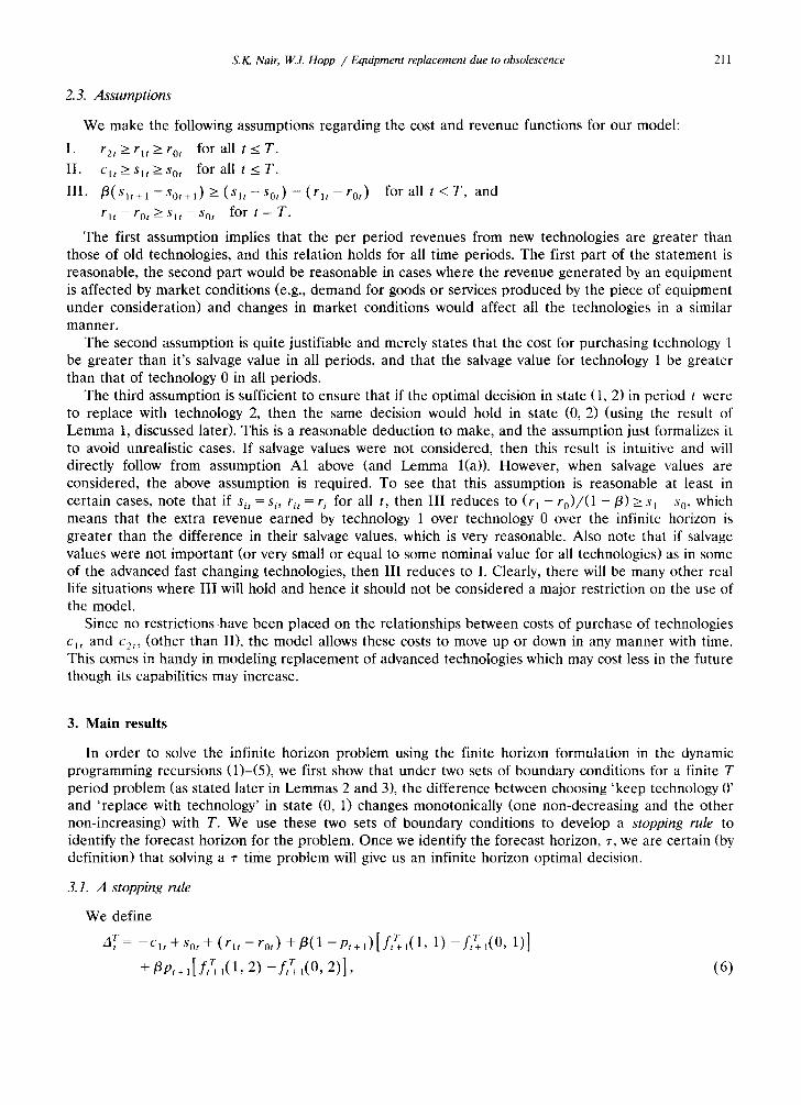
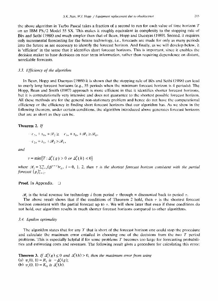
We present Figure 1 to put all our results up to now in perspective, and also to facilitate the understanding of the results and algorithm stated later. Notice that the forecast horizon is identified


80

60

40

20

A~ o

-20

--40

-60

~N,,NAr cn)

T Figure 1. Monotonicity of A T using boundary conditions of Lemmas 2 and 3. Data is from numerical example (a) in Section 3.6.

Here the optimal infinite horizon decision is ~-,(0, 1) = R 1, and the forecast horizon is ~" = 3

when both the curves are on the same side of Art = 0. W h e n they are on the positive side, the optimal decision is ~-t(0, 1) = R1, and when they are on the negative side, the optimal decision is rrt(0, 1 ) = K 0.

3.2. The algorithm

T h e o r e m 1 provides the basis for an algori thmic approach to comput ing the infinite horizon optimal ' k eep ' or ' r ep lace ' decision for any period, and specifically for t = 0. The algori thm can be stated as follows:

Step 1. Choose a small t ime horizon T (say T = 3), make forecasts Pt for periods 1 . . . . , T. Step 2. Solve two T-period problems:

• The first with boundary condit ions of L e m m a 2. One possible set could be: ~, L(0, 1) -- 0,

t> L(1, 1) = min[c l r - s0r, r l r - rot], ~> L(0, 2) --- 0, t> L(1, 2) = s i t - Sot, and t> L(2, 2) = c2r - So~.

• The second problem should have boundary condit ions of L e m m a 3. One possible set could be"

~, L(0, 1) = ~, L(1, 1) = t> L(0, 2) = t> L(1, 2) =

,

C l T - - SOT ,

O, C I T - - SOT , and

t> L(2, 2) = min[c2r - sir, rzr - rlr] + Clr - Sot. Step 3. For the per iod of interest, in this case t = 0, check to see if ei ther Art(g) > 0 in the first problem,

or Art(h)<_ 0 in the second problem. If yes, stop. ~" = T is the forecast horizon. The optimal decision in both the problems will be the same (from T h e o r e m 1) and the optimal decision is 7rt(0, 1) = 7rtr(0, 1). I f no, go to Step 4.

Step 4. There are two options: (a) Increment T by 1 and go to Step 1, or (b) Compute the maximum error f rom using the T period problem decision (using result of

Theo rem 3, s tated later). I f acceptable, stop. If not acceptable, go to (a).

This approach has three advantages. First, it is extremely simple to implement, since testing for forecast horizons merely requires solving two finite horizon dynamic programs. An implementa t ion of


the above algorithm in Turbo Pascal takes a fraction of a second to run for each value of time horizon T on an IBM P S / 2 Model 55 SX. This makes it roughly equivalent in complexity to the stopping rule of B~s and Sethi (1988) and much simpler than that of Bean, Hopp and Duenyas (1989). Second, it requires only incremental forecasting for the future technology, i.e., forecasts are made for only as many periods into the future as are necessary to identify the forecast horizon. And finally, as we will develop below, it is 'efficient' in the sense that it identifies short forecast horizons. This is important, since it enables the decision maker to base decisions on near term information, rather than requiring dependence on distant, unreliable forecasts.

3.3. Efficiency of the algorithm

In Bean, Hopp and Duenyas (1989) it is shown that the stopping rule of Bbs and Sethi (1988) can lead to overly long forecast horizons (e.g., 55 periods when the minimum forecast horizon is 4 periods). The Hopp, Bean and Smith (1987) approach is more efficient in that it identifies shorter forecast horizons, but it is computationally very intensive and does not guarantee to the shortest possible forecast horizon. All these methods are for the general non-stationary problem and hence do not have the computational efficiency or the efficiency in finding short forecast horizons that our algorithm has. As we show in the following theorem, under certain conditions, the algorithm introduced above generates forecast horizons that are as short as they can be.

Theorem 2. I f

-- C 2r ~- Sot - } -32 ~ -- C lr -}-Sot "~'C~I ~--- ~ 0 ,

--C2r "}-Sl'r -{-"~2 ~C~l'

and

r : min(T" Art(g) > 0 or Art(h) < 0}

where ,~i = ~,-:~([3'-*)ri,, i = O, 1, 2, then r is the shortest forecast horizon consistent with the partial forecast {p,},_ i.

Proof. In Appendix. []

.91 i is the total revenue for technology i from period r through o0 discounted back to period r. The above result shows that if the conditions of Theorem 2 hold, then r is the shortest forecast

horizon consistent with the partial forecast up to r. We will show later that even if these conditions do not hold, our algorithm results in much shorter forecast horizons compared to other algorithms.

3.4. Epsilon optimality

The algorithm states that for any T that is short of the forecast horizon one could stop the procedure and calculate the maximum error entailed in choosing one of the decisions from the two T period problems. This is especially helpful if for some problems T becomes too large for forecasting probabilities and estimating costs and revenues. The following result gives a procedure for calculating this error:

Theorem 3. I f Art(g) < 0 and Art(h)> O, then the maximum error from using (a) %(0, 1 )= R~ is -Art(g); (b) ~r,(0, 1 )= K o is Art(h).


Proof. The proof is straightforward from Lemmas 2 and 3. []

The intuition behind this result will be clear from Figure 1. Since Art(g) and AT(h) are bounds for A~, if we choose the decision based on one of these, the maximum error will be given by the (absolute value of the) other.

3.5. Sensitivity to changes in forecasts

Since the probabilities in this model are non-stationary in time, it would be useful to have results which could predict the optimal decision with changes in probabilities. For example, if a decision maker forecasts probabilities upto T = 5, and runs the algorithm to find that the optimal infinite horizon decision is to keep technology 0. It would be useful to know if this decision would change if the probability estimates were increased for some or all of the periods, without having to run the dynamic programs once again. We present one such result here after proving a technical lemma (which may be skipped by the casual reader).

Lemma 4. I f p = ( P t + I , P t + 2 , ' - ' , PT) and/~ = (/~t+l,/5,+2 . . . . , I~T) where Pi >Pi for all t < i < T, then Art(~) < AT(p), where Art(.) - T _ = A t when probability vector ( ' ) is used.

Proof. We know from Lemma l(c) that f~r(1, 1) - f,r(0, 1) _>fir(l, 2) --f tT(o, 2) for all t _< T. Hence from (6) we know that Atr is non-increasing in Pt+l. From (1)-(3) we can see that f iT(l , 1) - - f ,T (o , 1) is non-increasing in Pt+l and from (3)-(4) that f tr(1, 2)- - f , r (o , 2) is independent of Pt for all t. Hence it follows that f tT(l , 1) --ftT(o, 1) is non-increasing in Pm for all m > t + 1. Thus Art(/~) < Atr(p ). []

The above result states that when the probability forecasts are increased, the value of Art decreases (or more accurately, does not increase). This result helps in predicting the stability of the optimal decision, which we formally state in the result below.

Theorem 4. (a) / f 7rrt (p ) = Ko, then 7rT(~) = Ko; (b) I f 7rt~(~) = R 1, then Try(p) = R 1.

Proof. The result follows directly from Theorem 1 and Lemma 4. []

Theorem 4 implies that if the optimal decision is to ' keep ' using a particular technological forecast vector, then the optimal decision will be 'keep ' also for a technological forecast vector that stochastically dominates the original vector. This is entirely intuitive. The opposite holds if the optimal decision were to ' replace ' .

3.6. Numerical examples

We now discuss a few numerical examples to illustrate our algorithm for finding the optimal infinite horizon decision using the forecast horizon approach. Specifically, we are interested in ~-0(0, 1), the optimal infinite horizon decision in the initial period in state (0, 1).

Suppose r2t = 175, Czt = 200, sit = 75 and Sot = 35 for all t; T = 4 and /3 = 0.9. Let

roo = 50, r01 = 60, r02 = 45, ro3 = 50, r04 = 65,

rl0 = 100, r12 = 100, rlz = 95, rl3 = 90, r14 = 75,

c10 = 125, cll = 175, cl2 = 100, Cl3 = 100, C14 = 200.

Note that assumptions I - I I I are satisfied by the data. We use the boundary conditions stated in our algorithm in Section 3.2 to solve two dynamic programs.


80

60

40

20

A,' o

-20

4 0

-60

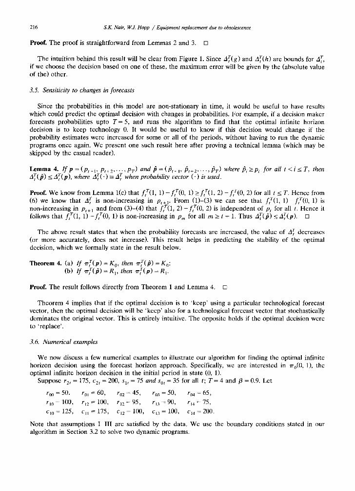
Figure 2. Resul ts from numerical example (b). Here

o

T the optimal infinite horizon decision is ~'t(0, 1 )= K 0 and the forecast horizon

is ~-=4

(a) Suppose the technological forecast were 191 = 0.1, P2 = 0.2, P3 = 0.3, P4 = 0.6. Using the boundary conditions in Lemmas 2 and 3 we have z l4(g)= 5 and A4(h)= 9, respectively. It follows from Theorem 1 that ~-0(0, 1) will be R x, and so, the decision to replace the current equipment with that presently available in the market is optimal for any technological forecast in period 5 and beyond. The values of zl0r(g) and A~(h) for different values of T are shown in Figure 1. It can be seen from Figure 1 that in this case the forecast horizon ~-= 3. When the time horizon is T = 4, as in this example, the same decision holds by definition of forecast horizons as we have above.

(b) If p~ = 0.5, P2 = 0.3, P3 = 0.3, P4 = 0 . 6 , then using the boundary conditions in Lemmas 2 and 3 we have A4(g) = - 1 6 and A4(h) = - 9 , respectively. It follows from Theorem 1 that ~-0(0, 1 ) = K 0 regardless of the forecast for periods 5 and beyond. Hence, one should keep the existing piece of equipment so as to replace it later when technology 2 appears. The forecast horizon is 7 = 4. The values of a~(g) and A~(h) for different values of T are shown in Figure 2.

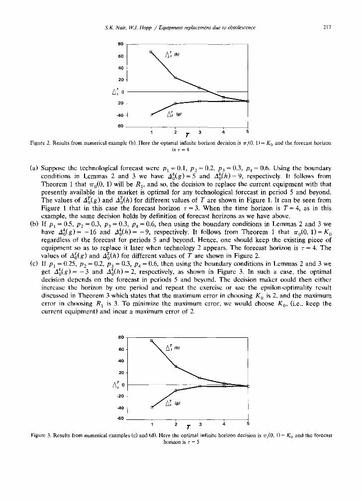
(c) If Pl = 0.25, P2 -- 0.2, P3 = 0.3, P4 = 0 . 6 , then using the boundary conditions in Lemmas 2 and 3 we get A4(g)= - 3 and A4(h)= 2, respectively, as shown in Figure 3. In such a case, the optimal decision depends on the forecast in periods 5 and beyond. The decision maker could then either increase the horizon by one period and repeat the exercise or use the epsilon-optimality result discussed in Theorem 3 which states that the maximum error in choosing K 0 is 2, and the maximum error in choosing R 1 is 3. To minimize the maximum error, we would choose K 0, (i.e., keep the current equipment) and incur a maximum error of 2.

80

60

40

20

o

-20

4 0

-60

Figure 3. Resul ts from numerical examples (c) and

o

T (d). Here the optimal infinite horizon decision is ~rt(0, 1)= K 0 and the forecast

horizon is 1- = 5

218 S.K. Nair, 14(J. Hopp / Equipment replacement due to obsolescence

(d) If, however, the decision maker in the previous case decides to increase T to 5 and forecasts the probability, costs and revenues to be P5 = 0.6, %5 = 85, ri5 = 85 and c15 =290, then we get ASo(g) = - 3 and A~(h)= - 3 as shown in Figure 3. Hence I -= 5 is the forecast horizon and using Theorem 1, 7r0(0, 1 )= K 0.

(e) Using Theorem 4 we can say that all forecast vectors that are dominated by the one in case (a) also will result in ~-0(0, 1 )= R 1 and all forecast vectors that dominate the one in case (b) and (d) will result in rr0(0, 1 )= K 0.

If in the above examples we let rit = ri4 and cit ~-Ci4 for all t > 4 and i = 0, 1, 2, then the first condition of Theorem 2 is not satisfied (as - c 2 r + s0r + ~ 2 = 1585, - c jr + SoT +--~l = 585, and ~ 0 = 650) and hence the forecast horizon obtained is not the shortest possible. It is interesting to note that the forecast horizon of 3 and 4 for our examples (a) and (b), respectively, is still appreciably shorter than that obtained by the method of B~s and Sethi (1988). To see this, we observe that for our problem, the B~s and Sethi stopping rule can be stated as follows:

Stopping rule (B~s and Sethi). If A~> ( I - c , 0 + s00 + rio I ) /3T/ (1- /3) , then ~-~t(0, 1 )= 7rS(0, 1) for all M>_T.

For example (a), A 4 = 7, and hence the forecast horizon works out to T = 36 using the Bbs and Sethi rule, whereas in our method the forecast horizon was T = 4. Other examples yield similar results. Thus, our simple method shows the same level of improvement over the B~s and Sethi method achieved by the much more complicated approach of Bean, Hopp and Duenyas (1989).

4. Conclusions

We have given a method for computing the optimal equipment replacement decision where the technological forecasts and cost and revenue functions are non-stationary. This method assumes that only one new technology may appear in the future in addition to the technology already available on the market at the current time. A few assumptions about the nature of revenue and cost functions have been made with a short discussion of situations where these assumptions would be justifiable.

The algorithm developed in this pape r is extremely simple computationally as well as to code, and, under certain conditions, is efficient in the sense of computing the optimal initial ' keep ' or ' replace ' action using a minimum number of periods of forecast data. Even when such conditions do not hold, the algorithm identifies forecast horizons that are much shorter and in lesser computational time than other existing methods.

Further work is needed to characterize the problem of equipment replacement when more than one alternative is available on the market at the outset, and the situation where more than one improvement can occur in the future. These situations do not lend themselves to choice of appropriate boundary conditions as was done in this paper. General -purpose methods can be used for these cases but such methods are cumbersome, as discussed earlier.

Appendix

Lemma 2. If

L(1 , 1 ) - L(D, 1 ) = min[clr-Sov, rlT--rOT],

L(1, 2) - L(0, 2) = s , T - Soy,

z.(2, 2) - L ( 1 , 2) =C2T--S,T,

then ay(g) is non-decreasing in T, where Art(g) - Art under these particular boundary conditions.


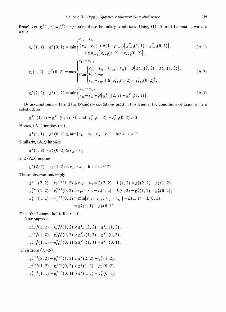
Proof. Let gf(', " ) - f f ( ' , • ) under these boundary conditions. Using (1)-(5) and Lemma 1, we can write

Clt -- SOt,

g,r(1, 1) -g,r(0, 1) = min{ ( r l t - ro , ) +/3(1-p,+l)[g,r+l(1, 1) - g r ~ ( 0 , 1)] (A.1)

[ +/3Pt+l[grt+,(1,2)-gf+l(O, 2)],

Slt -- SOt,

_ T = } ( c 2 ' - s ° t - ( r z t - r l ' ) - / 3 [ g T t + l ( 2 ' z ) - g T t + l ( l ' 2 ) ] '

Sot, gi'(1 2) g , (0 ,2) maX]min/q ' - (A.2)

[ ~ r l t - rot + f l [gTl( l , 2) --gtg+ 1(0, 2)],

gf(2, 2) - gf(1, 2) = min/c2' - sl ' ' -- gt+l( ,2)1 ~ r a t - - r l t + f l [ g L l ( 2 , 2) T 1 . (a.3)

By assumptions I-III and the boundary conditions used in this lemma, the conditions of Lemma 1 are satisfied, so

gLl(1, 1) -- g f+l (0 , 1) > 0 and gr l (1 , 2) --gTl(0 , 2) > 0 .

Hence, (A.1) implies that

g , r ( 1 , 1 ) - g f ( 0 , 1 ) > m i n [ c l t - s 0 , , q t - r 0 , ] f o r a l l t < T .

Similarly, (A.2) implies

gf(1, 2) - g f ( 0 , 2) ~'Slt--Sot

and (A.3) implies

gf(2, 2) - g f ( 1 , 2) <_cit-slt for all t < T.

These observations imply

gr+'(2, 2) -grr- l(1, 2) <c2r-Slr=L(2, 2) -L(1 , 2) =grr(2, 2) -grr(1, 2),

grr+l(l, 2) -grr+l(0, 2) >s,r-Sor=L(1, 2) -L (0 , 2) =grr(1, 2) -grr(0, 2),

gr+l(1, 1) -g r+ l (0 , 1) > min[qr-Sor, qr-ror] =L(1, 1) -L (0 , 1)

=grr(a, 1) -grr(0, 1).

Thus the Immma holds for t = T. Now suppose

gT++11(2, 2) -gT+ll(1 , 2) <gLl(2, 2) --gf+l(1, 2),

gT+ll(1 , 2) --gT~lt(0 , 2) _> gtT+l(1, 2) T -- g t + l ( 0 , 2 ) ,

g,r++ll(1, 1) -gf+ll(0, 1) >_gf+l(1, 1) r -- gt+l(0, 1).

Then from (7)-(9),

gf+l(2, 2) -g f+ l (1 , 2) < g,r(2, 2) - g f ( 1 , 2),

gf+l(1, 2) -g f+ l (0 , 2) >gr(1 , 2) - g f ( 0 , 2),

gT+l(1, 1) - -gT+l (0 , 1) >_grt(1, 1) --gT(O, 1).

220 S.K Nair, W..J. Hopp / Equipment replacement due to obsolescence

It follows by induct ion that gtr(1, 1) - g r ( 0 , 1) and g r (1 , 2) - g t r ( 0 , 2) are non-decreas ing in r . Thus using (6) A t ( g ) is non-decreas ing in T. []

Theorem 2. I f

--C2. r -~- SO, "t-~.~ 2 ~ --el. r "t- SOy -]-~1 ~ '~0 ,

- c 2 , + s l , + J i ' 2 >~a;'l,

and

~" = min{T: AtT(g ) > 0 o r ArT(h) < 0 }

where ~ i = ~ t = , ( ~ t - ' ) r i t , i = O, 1, 2, then .r is the shortest forecast horizon consistent with the partial

forecast {pt}[= 1.

Proof. We prove the result by showing that the bounda ry condit ions of L e m m a s 2 and 3 are consistent with actual forecasts for per iods ~-+ 1, z + 2 . . . . . Hence , if A t ( g ) < 0 or A t ( h ) > 0, then there are forecasts beyond r that lead to di f ferent decisions, so the initial decision depends on forecas t data beyond r and is not a forecas t horizon.

First we show tha t the bounda ry condit ions of L e m m a 2 are consis tent with any forecast tha t has P ,+ I = 1. Not ice that if p~+l = 1, then the--only states that are accessible beyond per iod r are (0, 2), (1, 2), and (2, 2). Thus, to show that this forecas t is consis tent with the boundary condit ions of L e m m a 2, it is sufficient to show that

f , ( 1 , 2) - f , ( 0 , 2) =S1,--So, and f , ( 2 , 2) - f , ( 1 , 2) = c 2 , - s l ,

where f , ( . , • ) r epresen t s the infinite hor izon value funct ion in per iod r. T h e condi t ion of the t heo rem guaran tees tha t for this forecast ( f rom expressions (3)-(5)) ,

f~(0, 2) = - c 2 , + s 0 , + ~ ' 2, L ( 1 , 2) = - c 2 , --[- Sl, --[-,~2, f~(2, 2) =,9/' 2,

so the result follows. Next we show tha t the boundary condi t ions of L e m m a 3 are consis tent with the forecast P ,+ l = P , + 2

. . . . . 0. Not ice that in this case t h e only states that are accessible beyond per iod ~- are (0, 1) and (1, 1). To show that this forecast is consis tent with the condi t ions in L e m m a 3, it is sufficient to show that f , (1 , 1) - f , ( 0 , 1) = Cl, - So,. F r o m the condi t ion of the t h e o r e m we have ( f rom expressions (1)-(2))

f~(0, 1 ) = - C l r at- s0, --1--,.~1 , L ( 1 , 1) ~--,-~1,

which comple tes the result. []

References

Bhaskaran, S., and Sethi, S. (1987), "Decision and forecast horizons in a stochastic environment: A survey", Optimal Control Applications and Methods 8, 201-207.

Bean, J., and Smith, R. (1984), "Conditions for the existence of planning horizons", Mathematics of Operations Research 9, 391-401.

Bean, J., Hopp, W., and Duenyas, I. (1989), "A stopping rule for forecast horizons in non-homogeneous Markov decision processes", TR 89-03, Dept. of Industrial Engineering and Management Sciences, Northwestern University, Evanston, IL.

B~s, C., and Sethi, S. (1988), "Concepts of forecast and decision horizons: Applications to dynamic stochastic optimization problems", Mathematics of Operations Research 13, 295-310.

Chand, S., and Morton, T. (1986), "Minimal forecast horizon procedures for dynamic lot size models", Naval Research Logistics 33, 111-122.

Chand, S., and Sethi, S. (1982), "Planning horizon procedures for machine replacement models with several possible replacement alternatives", Naval Research Logistics 29, 483-493.


Derman, C. (1963), "Optimal replacement and maintenance under Markovian deterioration with probability bounds on failure", Management Science 9, 478-481.

Goldstein, T., Ladany, S., and Mehrez, A. (1986), "A dual machine replacement model: A note on planning horizon procedures for machine replacement", Operations Research 34, 938-941.

Goldstein, T., Ladany, S., and Mehrez, A. (1988), "A discounted machine replacement model with an expected future technological breakthrough", Naval Research Logistics 35, 209-220.

Hatoyama, Y. (1984), "On Markov maintenance problems", IEEE Transactions on Reliability 33, 280-283. Hopp, W. (1987), "Identifying forecast horizons in nonhomogeneous Markov decision processes", Operations Research 35,339-343. Hopp, W., Bean, J., and Smith, R. (1987), "A new optimality criteria for nonhomogeneous Markov decision processes", Operations

Research 35, 875-883. Hopp, W., and Nair, S. (1991), "Timing equipment replacement decisions due to discontinuous technological change", Nat~al

Research Logistics 38, 203-220. Nair, S. (1988), "Replacement decisions due to technological obsolescence under uncertainty", Unpublished Ph.D. Thesis,

Department of Industrial Engineering and Management Sciences, Northwestern University, Evanston, IL. Pierskalla, W., and Voelker, J. (1976), "A survey of maintenance models: The control and surveillance of deteriorating systems",

Nat,al Research Logistics 23, 353-388. Sethi, S., and Chand, S. (1979), "Planning horizon procedures for machine replacement models", Management Science 25, 140-151.

a model for equipment replacement due to …webuser.bus.umich.edu/whopp/reprints/a model...

Documents