1

Auke Plantinga

Bert Scholtens

16005-EEF

The Financial Impact of Divestment

from Fossil Fuels

2

SOM is the research institute of the Faculty of Economics & Business at the University of Groningen. SOM has six programmes: - Economics, Econometrics and Finance - Global Economics & Management - Human Resource Management & Organizational Behaviour - Innovation & Organization - Marketing - Operations Management & Operations Research

Research Institute SOM Faculty of Economics & Business University of Groningen Visiting address: Nettelbosje 2 9747 AE Groningen The Netherlands Postal address: P.O. Box 800 9700 AV Groningen The Netherlands T +31 50 363 9090/3815 www.rug.nl/feb/research

SOM RESEARCH REPORT 12001

3

The Financial Impact of Divestment from Fossil

Fuels Auke Plantinga University of Groningen, Faculty of Economics and Business, Department Economics, Econometrics and Finance Bert Scholtens University of Groningen, Faculty of Economics and Business, Department Economics, Econometrics and Finance & School of Management, University of Saint Andrews l.j.r.scholtens@rug.nl

1

The financial impact of divestment from fossil fuels

Auke Plantingaa and Bert Scholtens

a,b,c

a Faculty of Economics and Business, Department of Economics, Econometrics

and Finance, University of Groningen, PO Box 800, 9700 AV Groningen, The

Netherlands.

b School of Management, University of Saint Andrews, The Gateway, North

Haugh, St Andrews, Fife, KY16 9RJ, Scotland, UK.

c Corresponding author. Email: l.j.r.scholtens@rug.nl; Phone: +31-503637064;

Fax +31-503638252.

2

The Financial Impact of Divestment from Fossil Fuels

Abstract

Divesting from fossil companies has been put forward as a means to address climate

change. We study the impact of such divesting on investment portfolio performance.

To this extent, we systematically investigate the investment performance of portfolios

with and without fossil fuel company stocks. We investigate mispricing in stock

returns and test for the impact of (reduced) diversification by excluding fossil fuel

companies from the portfolio. While the fossil fuel industry outperforms other

industries based on returns only, we show that this is due to the higher systematic risk

of this industry, as there is no statistically significant difference between the risk-

adjusted performance of stocks in the fossil fuel sample and the non-fossil fuel sample.

We conclude that divesting from fossil fuels does not have a statistically significant

impact on overall portfolio performance, and only a very marginal impact on the utility

derived from such portfolios. The policy implication is that investors can divest from

fossil fuels without significantly hurting their financial performance.

Keywords: Divestment, Fossil fuels, Investment management, Portfolio

performance, Stock market

JEL codes: G11, Q41

3

1 Introduction

Allen et al. (2009) and Meinshausen et al. (2009) suggest that most fossil fuel reserves should

be left unused in order not to exceed the 2°C threshold beyond which it seems impossible to

avoid dramatic climate change. Griffin et al. (2015) find that investors only show a small

negative reaction to news about ‘unburnable carbon’. Nevertheless, public initiatives and non-

governmental organizations asking investors to move their funds out of the fossil fuel industry

have mushroomed (see https://campaigns.gofossilfree.org/). Their hope is this will help

reduce greenhouse gas emissions. Cornell (2015) finds that divestment from fossil energy

companies would be costly for US university endowments and would reduce the size of the

endowment by 12.1% over a 50-year time frame. In our study, we focus on what would

happen to investors’ financial performance if they sold their stocks in fossil energy companies

and systematically investigate the impact of such divestment at the portfolio level. In general,

energy firms make up part of most individual and institutional investment portfolios. This is

not a surprise, as they constitute about 7.5% of the market value of the MSCI World Index.

We take an investment perspective and focus on the impact of divestment from fossil

fuel stocks on investment performance using mean-variance portfolio theory. As suggested by

Cornell (2015), excluding fossil fuel stock potentially deteriorates the performance of a

diversified portfolio, in particular when fossil fuel stocks show better than average returns.

Additionally, excluding fossil fuel stocks from the investment universe reduces diversification

opportunities, which may increase portfolio risk. In this paper we will address these issues

and consider the implications of excluding fossil fuel stocks on portfolio performance in terms

of expected returns and risk.

The call for divestment from fossil fuels is related to socially responsible investing

(SRI). SRI focuses on how investors align ethical and financial concerns, as well as on the

4

impact on firms’ environmental, social, and governance (ESG) performance (Renneboog et

al., 2008). To achieve this, the socially responsible investors have developed a variety of

strategies, including “best-in-class” investing, active ownership, and ESG integration (see

Eurosif, 2014). However, the original SRI practice of excluding stocks of companies involved

in harmful or controversial activities (so-called sin stocks) remains the most common SRI

strategy today (see Eurosif, 2014). But what does it actually mean for an investor to employ

negative screens on the universe of potential investments, from the investment perspective?

And does it matter for financial performance if a ‘fossil’ screen is employed? Screening limits

the investment universe, which should be detrimental for the mean–variance efficiency of a

portfolio. For example, Hong and Kacperczyk (2009) find that investors who ditch firms in

contested industries like alcohol, tobacco and gambling forego the excess returns as these ‘sin

stocks’ have higher expected returns than similar stocks. The former being neglected by

investors who are constrained by norms and values. In contrast, Bello (2005) reports that

mutual funds with an SRI strategy have the same performance as a group of non-SRI funds

with similar characteristics; more recent studies (e.g. Humphrey and Tan, 2014) confirm this

findings. This is in line with the literature on the minimum number of stocks needed to create

a well-diversified portfolio, which claims that a limited number of stocks is sufficient. For

instance, this minimum is 10 stocks according to Evans and Archer (1968), and 40 according

to Statman (1987). This literature suggests that the exclusion of a small set of assets may have

only a minor impact on portfolio performance.

Our paper focuses on the financial performance of fossil fuel stocks in comparison

with all other industries and on the consequences of divestment from fossil fuel for portfolio

construction. We address the following two research questions:

1. Do returns from investing in fossil fuel stocks differ from those in other industries?

5

2. Are there implications for the performance of investment portfolios with and without

fossil fuel stocks?

We aim to contribute to the investment portfolio performance literature as well as the

responsible investment literature, since we investigate the potential downside on portfolio

choice of excluding fossil fuel stocks. This is the first study, to our knowledge, that

systematically investigates the impact of excluding fossil fuel stocks at the portfolio level. To

answer the research questions, we create two portfolios using standard industry indices

provided by Datastream. To address the first research question, we create a portfolio with all

fossil fuel stocks and one with all remaining stocks. Next, we analyze the returns of each

portfolio as well as the difference between them using the Carhart (1997) extension of the

Fama and French (1993) model. Since the second research question focuses on investment

portfolios, we construct optimal portfolios using mean variance optimization to assess the

impact of screening on fossil fuel stocks.

We find that both the fossil fuel stocks and all remaining stocks are priced consistent with

the Carhart (1997) model. In addition, the difference in returns between the fossil fuel and

other stocks does not generate a significant risk-adjusted return, although there are statistically

significant differences in exposure to systematic risk. Further, we find that limiting the

investment universe by excluding fossil fuel stocks has a marginal impact on the performance

of a portfolio. The financial performance of the restricted portfolios with lower risk tends to

have lower utility for the investor than the unrestricted portfolios; vice versa, the restricted

portfolios with higher risk have higher utility than the unrestricted portfolios with higher risk.

This paper proceeds as follows. We describe the sampling process and the data in

Section 2. We present the findings in Section 3. Here, we also discuss the implications of

these results, particularly in light of the divestment and screening discussion. We set forth our

conclusions in Section 4.

6

2 Materials and methods

We test the impact of excluding fossil fuel stocks from the investment universe by

studying stock returns at the industry level. This is because such an approach is easily

translated into an investment strategy, with no liquidity concerns. Many providers offer

industry-level portfolios as actively managed mutual funds, passively managed mutual funds,

or exchange traded funds, which makes it easy for an investor to implement the strategies that

we investigate. We use the industry indices provided by Datastream, as they have a return

history of more than 40 years, allowing for elaborate robustness analysis. The Datastream

industry indices are based on the Industry Classification Benchmark (ICB) for classifying

stocks into industries and sectors, which include four hierarchical classification levels: the top

level is industry, and the remaining levels are supersector, sector, and subsector, respectively.

In our study, we focus on the top level, which consists of ten industries. Industry-level

classification plays an important role in the practice of investment management. Many

professional investment institutions follow industry classification in their investment

processes, by focusing on specific industries or by defining their asset allocations in terms of

industry. We adjust the ICB classification by relocating some (sub)sectors. There are two

reasons for doing so. First, companies involved in the exploration and exploitation of fossil

fuels are present in two different industries, namely the ICB industries Oil and Gas and Basic

Materials. Second, the ICB industry Oil and Gas also contains the sector of Alternative

Energy stocks. Therefore, we create a new industry classification that replaces the initial

industry Oil and Gas with the newly created industry Fossil Fuels. This Fossil Fuels index

consists of the sectors Oil and Gas Producers and Oil Equipment and Services from the Oil

and Gas industry and the subsector Coal Mining from the Basic Materials industry. This new

index has 327 constituents. We create an adjusted Basic Materials index, which is based upon

the ICB Basic Material index, excluding stocks of firms involved in coal mining activities.

7

We adjust the Utilities index by adding the sector Alternative Energy, which is separated from

the Oil and Gas industry. Finally, we also create a new index, the All Stocks Excluding Fossil

Fuel Index (ASEFFI). This index has 6,578 constituents, being the sum of all other indices

except for the Fossil Fuel Index. We summarize this transformation of the industry indices in

Table I. We want to point out that this approach is very well in line with what is being used in

the investment industry (see e.g. FTSE Russell, 2014).

Table I. Definition of new industry indices

New industry

definition

# Consti-

tuents

Link with original

ICB industry

(Sub)sector

Fossil Fuels 327 Oil and Gas

Basic Resources

Oil & Gas Producers (sector)

Oil Equip. & Serv. (sector)

Coal (subsector)

Basic Materials 460 Basic Materials All (sub)sectors except for

coal

Industrials 1,297 Industrials Unchanged

Consumer Goods 914 Consumer Goods Unchanged

Health Care 402 Health Care Unchanged

Consumer Services 900 Consumer Services Unchanged

Telecom 153 Telecom Unchanged

Utilities 332 Utilities

Oil & Gas

All (sub)sectors

Alternative Energy

Financials 1,731 Financials Unchanged

Technology 389 Technology Unchanged

ASEFFI 6,578 All Stocks Excluding Fossil Fuels

We collected monthly total returns for all of the indices starting from January 1973

until March 2015. Table II presents the summary statistics of the returns for all the (adjusted)

industries, including the Fossil Fuels index (FFI), and the adjusted Basic Materials and

8

Utilities indices. The other industries (Industrials, Consumer Goods, Health Care, Consumer

Services, Telecommunications, Financials, and Technology) remain unchanged. The adjusted

industry indices as well as the ASEFFI are constructed as portfolios of industries and/or

(sub)sectors. The weights are based on the market capitalizations of the underlying industry,

sector, or subsector. Portfolios are rebalanced monthly, and the return of an index is

calculated as the market capitalization weighted average return of all industries in the index.

The returns for the unadjusted indices are directly retrieved from Datastream. All returns

index prices are denominated in US dollars and the resulting returns are denominated in

percentages.

Table II shows that the fossil fuel industry has the highest average mean return over

the period 1973–2015. This supports the notion that excluding fossil fuel stocks might have a

detrimental impact on portfolio performance. Moreover, if there were some index that showed

better performance than this index, this would suggest that replacing the former by the latter

would create financial value for the investor. We will investigate this issue in the next section.

Table II shows that the consumer goods industry has the lowest performance. The difference

between the best and worst performing industries is 0.22% over the period 1973–2015, thus,

we may conclude that the differences in returns between individual industries are quite

limited. The technology industry has the highest monthly standard deviation (6.54%) and the

health care industry the lowest standard deviation (4.05%). Therefore, differences in standard

deviations between individual industries are also limited, although they are somewhat bigger

than the mean return differences. In Table A.1 in the Appendix, we provide the results for

subperiods. These suggest that the average return for stocks in the fossil fuel index (FFI) have

tended to decline over the past 20 years.

9

Table II. Summary statistics for returns of industry indices

This table presents average, median and standard deviations of monthly returns

starting from January 1973 until March 2015.

1973-2015

Mean Median Standard

deviation

Fossil Fuels 1.06% 1.04% 5.63%

Basic Materials 0.92% 1.09% 5.85%

Industrials 0.94% 1.24% 5.09%

Consumer Goods 0.85% 1.00% 4.88%

Health Care 1.03% 1.09% 4.05%

Consumer Services 0.84% 1.03% 4.68%

Telecommunications 0.91% 0.83% 5.02%

Utilities 0.89% 0.92% 4.29%

Financials 0.94% 1.22% 5.58%

Technology 0.98% 1.04% 6.54%

ASEFFI* 0.88% 1.14% 4.57%

All industries 0.89% 1.20% 4.54%

*All Stocks Excluding Fossil Fuel Index.

To investigate the impact of divesting from fossil fuel stocks on investment

performance, we must address differences in risk between industries and assess the

implications for risk from creating a diversified portfolio. One of the main explanations for

the differences in mean returns between industries is differences in systematic risk. At the

same time, we should also consider the benefits from creating a diversified portfolio.

Accordingly, we estimate an asset pricing model to address the issue of risk, and we create

efficient portfolios to assess the diversification costs of excluding fossil fuel stocks.

The first research question we address regards comparison of returns from fossil fuel

investing versus investing in other industries. Although the summary statistics suggest that

10

fossil fuel stocks have higher returns than other industries, the difference could be explained

by risk. We answer this question by performing Fama and French (1993) regressions extended

with the momentum factor proposed by Carhart (1997); this is currently the mainstream

standard asset pricing model. In this model, the return ��,�on a portfolio p in month t is

explained by the following regression:

��,� = � + �,��,� − � ,�� + �,�����,� + �,�����,� + �,���,� + ��,� (1)

where �,� is return on the market portfolio and ���,� is the return the so-called SMB factor,

a long portfolio in small cap stocks and short portfolio in large cap stocks. Furthermore,

���,�, is the return on the HML factor, a portfolio with positive weights in stocks with a high

book-to-market ratio and negative weights in a portfolio with low book-to-market ratios, and

finally, ��,� is the return on the momentum factor, a portfolio with positive weights in

stocks with the highest returns and negative weights in stocks with the worst performance in

the past 12-months. The market portfolio and factor-mimicking portfolios are global factors

obtained from the website of Kenneth French.1 Since these factors are available only starting

from July 1990, equation (1) is estimated using data from November 1990 to March 2015.

Using regressions of this type is frequently done in empirical research to test alternative

investment strategies (see, e.g., Banerjee et al., 2007; Goyal, 2012).

The second research question investigates the impact of a limited universe on the

diversification opportunities and the performance of a portfolio with and without fossil fuel

stocks. With a well-diversified portfolio, it is possible to attain lower levels of risk at a given

level of expected return. We compare the differences between the performance of the two

portfolios using the Sharpe (1966) ratio, which provides a convenient way to compare

portfolios with different levels of risk. However, this approach relies on perfect markets,

1 http://mba.tuck.dartmouth.edu/pages/faculty/ken.french/index.html

11

where investors can borrow and lend at one riskless rate without limits. In practice, investors

are limited in so doing. An alternative way of addressing the second research question is to

examine the return differences of investment strategies with and without fossil fuel stocks. To

this extent, we choose to model a limited set of passive strategies linked closely to standard

portfolio theory. We use a two-step approach in testing each strategy. In the first step, we

estimate the input parameters for the strategy based on returns from the estimation period,

which is a period of 60 months preceding the moment of portfolio construction. In the second

step, we calculate the portfolio resulting from these parameter choices, and implement this on

the first day after the estimation period. This portfolio is passively managed without being

adjusted to new information for the next 60 months following the estimation period. We track

the performance of the portfolio during these 60 months, while rebalancing the weights of the

portfolio on a monthly basis to keep them aligned with the portfolio weights initially

calculated.

Since the main benefit of diversification is risk reduction, we begin by focusing on the

minimum variance portfolio. Since it represents the portfolio with the lowest risk, the

minimum variance portfolio is a natural measure of the risk-reduction potential in a universe

of risky assets. It is constructed without the need to estimate expected returns and is based on

the covariance matrix of returns only. As a result, its composition is associated with less

estimation risk than, for instance, a tangency portfolio. The tangency portfolio is constructed

by optimizing the Sharpe ratio, which is the portfolio return in excess over the risk-free rate as

a fraction of its standard deviation. The calculation of the composition of the tangency

portfolio requires the covariance matrix and the expected returns. Among others, Best and

Grauer (1991) and Chopra and Ziemba (1993) show that estimation risk is an important

consideration in finding optimal portfolios, in particular when it comes to estimating expected

12

returns. The minimum variance portfolio for period � is calculated using the following

expression:

�� =����

������, (2)

where Ω is the full historical covariance matrix estimated over the estimation period � − 1

preceding the time of portfolio construction and � is a vector of ones.

The main analysis is an out-of-sample test using an estimation period and an

evaluation period, because this represents a feasible strategy for any investor, relying only on

information that is available at the time of portfolio construction. During the estimation

period, we estimate the covariance matrices and use these to construct portfolios at the

beginning of the evaluation period. We measure the performance of the portfolio over the

evaluation period. A common approach to calculating optimal portfolios is to use five years of

historical data (see Chan and Lakonishok, 1999). This pragmatic choice represents a trade-off

between the idea that parameters need to be estimated on a period as long as possible, while at

the same time the period can be too long because firms may change in terms of fundamental

risk and return characteristics. Therefore, we divide the data into eight periods of five years

each. This creates seven independent evaluation periods, since the first period is used as the

estimation period. The first period includes the monthly returns from January 1973 to March

1980. As such, the first portfolio is created on April 1st 1980, based on the historical

covariance matrix estimated over the period January 1973 to March 1980. The next portfolio

is created on April 1st 1985, based on the historical covariance matrix estimated over the

period April 1980 to March 1985, and so on.

We also construct portfolios with higher levels of risk than those implied by the

minimum variance portfolios. Accordingly, we calculate the tangency portfolio for period �

using the following equation:

13

�� =����

����� , (3)

where ! is the vector of excess returns. Excess returns are the difference between expected

returns and the risk-free rate. We use return on US Treasury bills as the risk-free rate. We also

create two more risky portfolios assuming the absence of a risk-free rate. We construct these

portfolios by maximizing the following preference function, which is equivalent to

maximizing an exponential utility function based on von-Neuman-Morgenstern preferences if

returns are jointly normally distributed (Freund, 1956):

"#$% = "&�' − (

)*+,, (4)

where �- is the risk tolerance of the investor. This preference function is a convenient way to

model the preferences of an investor in a mean-variance framework . The resulting measure of

utility is a certainty equivalent return, which can be easily compared across investment

alternatives. For instance, an investor with a risk tolerance of ‘1’ calculates a certainty

equivalent of 7% for an investment opportunity with an expected return of 8% and a standard

deviation of 10%. The certainty equivalent of the same investor is 6% for an investment with

an expected return of 6% and a standard deviation of 20%. As a result, the investor chooses

the first opportunity over the second one. Using the certainty equivalent provides a simple

economic interpretation: when the utility measure is below the risk-free rate, the investment

opportunity is inferior to an investment in the riskless asset.

Both approaches for calculating portfolios with higher risk levels require estimating

expected returns. Among others, Chan and Lakonishok (1999) and Chopra and Ziemba (1993)

argue that historical mean returns are much more difficult to predict than covariances, and

erroneous estimates could lead to highly inefficient portfolios in an out-of-sample test. To

mitigate the impact of estimation errors on portfolio choice, we estimate expected returns

14

using an asset pricing model. Jorion (1991) shows that using expected returns derived from a

capital asset pricing model (CAPM) is preferred over the historical mean. Preferably, we

would want to use the Fama and French (1993) model extended with the momentum factor.

However, due to lack of availability of global Fama and French factors for the period 1973 to

1990, we choose to use CAPM estimates as suggested by Jorion (1991). For each industry, we

estimate its beta relative to the MSCI All Countries World Index for each individual

subperiod:

".!�/ − ! = �� + ��"&!' − ! � + � (5)

The expected market return is calculated as the average return on the MSCI All

countries World Index over the period 1973 to 2015, and the risk-free rate is the average risk-

free rate downloaded from the website of Kenneth French. Following Jorion (1991), the

estimated betas can be used directly to infer optimal portfolio weights. We assess the

performance of all outcomes by comparing the means and standard deviations of the

portfolios with and without fossil fuel stocks using a paired t-test for the means and a Bartlett

test for the hypothesis of equal variances, which has an 0, distribution with one degree of

freedom.

We also provide in-sample results, which means that we calculate the composition of

the efficient portfolios at the beginning of the estimation period. This is the outcome of a

strategy where the investor has prior knowledge of future return distribution. The reason we

present the in-sample outcomes is that they provide an indication of the impact of limiting

diversification opportunities in the absence of parameter uncertainty. Without parameter

uncertainty, limiting the investment universe must, by definition, result in certainty equivalent

losses because of higher risk and/or lower return.

15

Finally, we evaluate the increase in mean variance efficiency of having a constrained

investment universe by calculating the certainty equivalent for each portfolio based on

equation (4). Next, we calculate the difference between the certainty equivalent for the

portfolio without fossil fuel stocks and the portfolio with all stocks. If the certainty equivalent

for the portfolio without fossil fuel stocks is lower than the portfolio with all stocks, the

restriction results in an efficiency loss. This procedure is in line with Chopra and Ziemba

(1993), who calculate the certainty equivalent loss in a similar way. It allows us to evaluate

the joint impact of a restricted investment universe on both return differences and

diversification opportunities.

16

3 Results

3.1 Fossil fuel stocks versus other stocks

Based on the discussion above , we now present the results of our analysis and address

the two research questions. We begin by investigating whether the returns from investing in

fossil fuel stocks differ from those of other industries. To this extent, we show the results of

estimating regression (1) using monthly returns from November 1990 through March 2015.

We estimate the model to explain the excess returns on ASEFFI. We test the hypothesis that

the risk-adjusted returns of both groups of stocks are similar by taking the difference between

the returns of the FFI and ASEFFI and explaining these differences using regression (1). The

results are presented in Table III. Panel A in this table shows that the risk-adjusted returns of

fossil fuel stocks are not significantly different from those of other stocks. Further, it shows

that fossil fuel stocks have significantly higher exposure to the SMB and the HML factors in

the Carhart model. This implies that the higher returns for fossil fuel stocks reported in Table

II are due to higher systematic risk.

17

Table III. Risk-adjusted returns for fossil fuel stocks versus other stocks

Panel A: OLS estimates of extended Fama and French model

This table provide Ordinary Least Squares (OLS) estimates of the regression

coefficients for the Carhart (1997) model using monthly returns from November 1990

to March 2015. Values in parentheses present t-values. *

, **

and ***

denote significance

at 10%, 5%, or 1% probability level, respectively.

FFI ASEFFI FFI-ASEFFI

� -0.000 0.001 -0.001

(0.03) (0.89) (0.36)

�, 1.042***

1.021***

0.021

(19.23) (50.34) (0.39)

�,�� 0.260**

-0.039 0.299***

(2.36) (0.93) (2.72)

�,�� 0.476***

-0.057 0.532***

(4.68) (1.49) (5.25)

�,� 0.029 -0.038 0.067

(0.48) (1.66) (1.11)

R2 0.58 0.91 0.10

18

-Table III continued-

Panel B: Estimates for the Carhart (1997) model using GARCH(1,1) model

This table provides Maximum Likelihood estimates of the regression coefficients for

the mean and variance specification of the Carhart (1997) model using monthly returns

and a GARCH(1,1) specification from November 1990 to March 2015. Values in

parentheses present t-values.

*,

** and

*** denote significance at 10%, 5%, or 1%

probability level, respectively.

FFI*

ASEFFI**

FFI-ASEFFI

Mean specification: ��,� = � + �,��,� − � ,�� + �,�����,� +

�,�����,� + �,���,� + ��,�,

� -0.001 0.001 -0.001

(0.29) (1.55) (0.41)

�, 1.016**

0.992**

0.005

(18.33) (55.62) (0.09)

�,�� 0.171 -0.032 0.146

(1.56) (0.98) (1.52)

�,�� 0.471**

-0.085*

0.429***

(4.79) (2.41) (5.22)

�,� 0.015 -0.020 0.023

(0.25) (0.96) (0.39)

Variance specification: ℎ� = �2 + �(��3(, + �,ℎ�3(

,

�2 0.000 0.000 0.000

(1.25) (2.04)* (1.43)

�( 0.133 0.192 0.194

(2.64)**

(4.26)***

(2.84)**

�, 0.836 0.760 0.783

(13.09)***

(16.75)***

(12.39)***

* Fossil Fuel Index

** All Stocks Excluding Fossil Fuels

19

The residuals from the regression models test positive on Arch effects using the

ARCH-LM test. For this reason, we also estimate a GARCH(1,1) model. The results are

reported in panel B of Table III and are quite similar to those in panel A. The main conclusion

from Table III is that the ten industries are priced in line with the extended Fama and French

(1993) model, with none of the constants statistically significant. Fossil fuel stocks have a

significantly higher loading on the HML factor relative to other stocks. The loading on the

SMB is only significantly higher for the OLS regression results and not for the GARCH(1,1)

model.

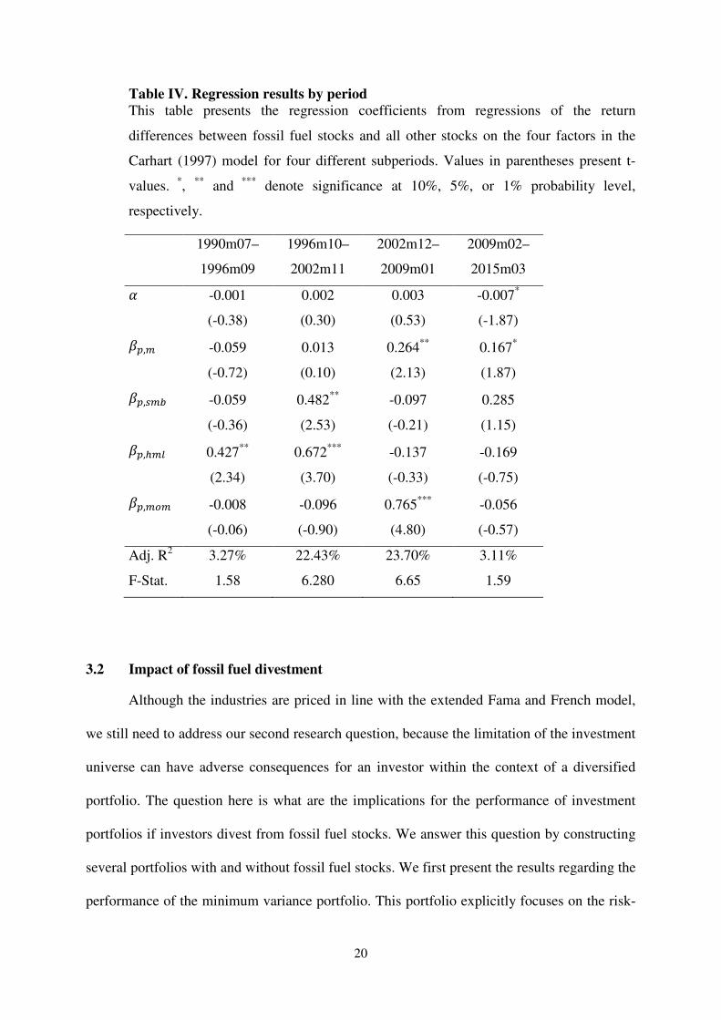
As a robustness check, Table IV presents the estimation results of the regression

explaining the return differences between fossil fuels stocks and all other stocks in four

subperiods of equal length.2 This table supports the main conclusion, namely, that investment

performance of the fossil fuel industry does not significantly differ from an investment

universe without fossil fuel stocks over a prolonged period of time. However, the risk-

adjusted returns on fossil fuel stocks are negative and marginally significant in the final

period. Exposure to systematic risk varies over time, where fossil fuels in comparison with the

other stocks have only higher exposure to the HML factor in the first two periods, higher

exposure to the SMB factor in the second period, and higher exposure to momentum stocks in

the third period.

2 The first period has only 71 months, due to data availability.

20

Table IV. Regression results by period

This table presents the regression coefficients from regressions of the return

differences between fossil fuel stocks and all other stocks on the four factors in the

Carhart (1997) model for four different subperiods. Values in parentheses present t-

values. *

, **

and ***

denote significance at 10%, 5%, or 1% probability level,

respectively.

1990m07–

1996m09

1996m10–

2002m11

2002m12–

2009m01

2009m02–

2015m03

� -0.001 0.002 0.003 -0.007*

(-0.38) (0.30) (0.53) (-1.87)

�, -0.059 0.013 0.264**

0.167*

(-0.72) (0.10) (2.13) (1.87)

�,�� -0.059 0.482**

-0.097 0.285

(-0.36) (2.53) (-0.21) (1.15)

�,�� 0.427**

0.672***

-0.137 -0.169

(2.34) (3.70) (-0.33) (-0.75)

�,� -0.008 -0.096 0.765***

-0.056

(-0.06) (-0.90) (4.80) (-0.57)

Adj. R2 3.27% 22.43% 23.70% 3.11%

F-Stat. 1.58 6.280 6.65 1.59

3.2 Impact of fossil fuel divestment

Although the industries are priced in line with the extended Fama and French model,

we still need to address our second research question, because the limitation of the investment

universe can have adverse consequences for an investor within the context of a diversified

portfolio. The question here is what are the implications for the performance of investment

portfolios if investors divest from fossil fuel stocks. We answer this question by constructing

several portfolios with and without fossil fuel stocks. We first present the results regarding the

performance of the minimum variance portfolio. This portfolio explicitly focuses on the risk-

21

reduction benefits of diversification, since this portfolio has the lowest risk given the

covariance structure.

Table V presents the estimation results regarding the out-of-sample performance of the

minimum variance portfolios. For most subperiods, the difference between the returns on

portfolios based on all assets and those based on all assets excluding fossil fuel stocks is very

small. There are some exceptions, however. During the period 1995–2000, the monthly return

of portfolios including fossil fuel stocks exceeds that of portfolios excluding fossil fuel stocks

by 0.25%, which is marginally statistically significant. This difference implies that when both

portfolios have the same value at the start in 1995, the value of the portfolio excluding fossil

fuel stocks is 24% lower compared to the portfolio with all stocks at the end of 2000.

While out-of-sample results are most relevant from a practical point of view, it may be

instructive to see some in-sample results. We have calculated the returns from the minimum

variance portfolio constructed at the beginning of the estimation window using the covariance

structure from the estimation window. These results can be interpreted as being representative

for a world where covariance matrices and expected returns are stationary and are known

beforehand without any estimation uncertainty. These results, which are presented in

Appendix Table A.2, show that restricting the investment universe indeed increases the risk of

the minimum variance portfolio. However, the differences in monthly standard deviations are

very small: the difference in standard deviation between other stocks and fossil fuel stocks is

3 basis points in the first period, and becomes 10 and 15 basis points, respectively, in the

periods 1995–2000 and 2010–2015. Thus, even in the theoretical case where estimation errors

can be avoided, the elimination of fossil fuel stocks only has a limited impact on risk

reduction.

22

Table V. Return on minimum variance portfolios with and without fossil fuel

stocks

This table presents out-of-sample average returns from investing in a minimum

variance portfolio with and without stocks related to the fossil fuel industry. It also

present the difference in mean return and the associated paired t-test. The monthly

standard deviation of the asset returns is presented in parentheses, as is the Bartlett test

statistic of equal variances. *,

** and

*** denote significance at 10%, 5%, and 1%

probability level, respectively.

Period

All assets

Excl. fossil

fuels

Difference in

mean returns

Diff. test t-test

(chi2)

1980–1985 1.73% 1.79% 0.06% -0.74

(3.73%) (3.82%) (0.04)

1985–1990 1.63% 1.64% 0.01% -0.43

(4.20%) (4.24%) (0.00)

1990–1995 1.10% 1.14% 0.03% -0.26

(3.01%) (3.23%) (0.30)

1995–2000 1.48% 1.22% -0.25% 1.96**

(4.30%) (4.20%) (0.04)

2000–2005 0.42% 0.41% -0.01% 0.48

(3.35%) (3.35%) (0.00)

2005–2010 0.64% 0.61% -0.03% 0.65

(3.90%) (3.91%) (0.00)

2010–2015 1.80% 1.64% -0.15% 1.37

(3.26%) (3.08%) (0.17)

Table VI presents the out-of-sample results for the tangency portfolios; it presents both

mean returns and standard deviations. In general, the differences between both portfolios in

terms of means and standard deviation tend to be small. The portfolios including fossil fuels

have statistically significant higher out-of-sample returns in the period 2010–2015 and have

marginally significant higher returns in the period 1995–2000. However, in economic terms,

23

the difference in performance is very limited as it translates into only 6 basis points per month

for 1995–2000 and 8 basis points for 2010–2015.

Table VI. Performance of tangency portfolios with and without fossil fuel stocks

This table presents out-of-sample average returns and standard deviations from investing

in the tangency portfolio with and without stocks related to the fossil fuel industry. It also

presents the difference in mean return and the associated t-test on the difference in mean

returns. The monthly standard deviation of returns is presented in parentheses. The table

also presents the Bartlett test statistic of equal variances in parentheses. *,

** and

*** denote

significance at 10%, 5%, or 1% probability level, respectively.

Period

All assets

Excl. fossil

fuels

Difference in

mean returns

Diff. test

t-test

(chi2)

1980–1985 1.36% 1.42% 0.07% -0.69

(3.46%) (3.34%) (0.08)

1985–1990 1.79% 1.84% 0.05% -0.48

(4.48%) (4.58%) (0.03)

1990–1995 0.78% 0.78% 0.00% 0.07

(4.05%) (4.20%) (0.08)

1995–2000 1.38% 1.32% -0.06% 1.86*

(3.91%) (3.92%) (0.00)

2000–2005 0.03% 0.05% 0.02% -0.53

(4.70%) (4.70%) (0.00)

2005–2010 0.72% 0.74% 0.02% -0.60

(5.85%) (5.76%) (0.01)

2010–2015 0.74% 0.67% -0.08% 2.26**

(4.51%) (4.53%) (0.00)

The risk of the portfolio excluding fossil fuel is sometimes higher (e.g., during the

period 1990–1995, the portfolio without fossil fuel had 15 basis points more risk), and

sometimes lower (e.g., during the period 2005–2010, the portfolio without fossil fuel had 9

basis points less risk). None of the differences between the pairs of standard deviations is

24

statistically significant, as is indicated in the column labeled “Diff. Test,” which presents the

Bartlett test statistic.

Summarizing both the evidence on the minimum variance portfolios and the tangency

portfolios, it is reasonable to conclude that screening for fossil fuel stocks and excluding them

from the investment portfolio has almost no impact on the returns of a globally diversified

portfolio of industry indices, although there is weak evidence that including fossil fuel stocks

may improve a portfolio’s performance.

3.3 Utility and constraining the investment universe

In the above analyses, we examine separately the impact of excluding fossil fuel

stocks from the investment universe in terms or return and risk. To study the joint impact on

return and risk, we calculate certainty equivalents according to equation (4). This approach

also allows us to study the impact of the restriction on higher levels of risk. To provide a

better understanding of the impact of excluding fossil fuel stocks on portfolios with different

risk levels, we calculate two sets of portfolios using different risk tolerance (RT) coefficients,

one using RT = 1 and the other RT = 2. The portfolios based on a RT = 1 are less risky than

the tangency portfolio, while the portfolios based on RT = 2 are more risky than the tangency

portfolio.

We calculate certainty equivalents based on the out-of-sample average returns and

standard deviations of both strategies. The outcomes are presented in Table A.3 of the

Appendix. These results are consistent with the previous results in the main analysis. The

differences in mean return between the investment universe including all assets and the

investment universe excluding fossil fuel stocks ranges between minus 8 basis points and plus

9 basis points, for a risk tolerance coefficient of 1. During the first two subperiods, excluding

fossil fuel stocks increases the mean return by 8 basis points, while, in the last period,

25

excluding fossil fuel stocks decreases the mean return by 9 basis points or less for a risk

tolerance coefficient of 1. For investors with a higher level of risk tolerance, the differences

are larger. The largest difference occurs in the period 1995–2000, when the portfolio

excluding fossil fuel stocks outperforms, at a statistically significant level, the unrestricted

portfolio by 34 basis points. However, risk, as measured using standard deviation during this

period, is also higher than during other periods.

By comparing the difference in the certainty equivalents of portfolios with and without

fossil fuels, we arrive at a measure of efficiency gains from excluding fossil fuels. The

certainty equivalent gains are presented in Table VII. Panel A shows the results for a risk

tolerance coefficient of 1. The restriction on the investment universe results in an average

utility loss of 0.05% for the minimum variance portfolio and as a result of the restriction on

fossil fuel stocks. Given this same risk tolerance coefficient, the utility loss for the tangency

portfolio is, on average, zero, while there is actually a utility gain of 0.03% for the portfolio

with risk level RT = 1. Overall, these results show that imposing a restriction on fossil fuel

stocks has only a modest impact on utility. The impact is negative for investors with low risk

tolerance and positive for investors with high risk tolerance.

Panel B of Table VII shows the results for an investor with a risk tolerance coefficient

of 2. Although we observe the same pattern, the differences are greater than in Panel A. The

investor experiences a utility loss of, on average, 0.13% for the minimum variance portfolio,

and 0.07% for the tangency portfolio, while the restriction results in substantial gains for the

portfolios constructed with RT = 2. At the same time, we observe that the pattern of utility

gains and losses shows substantial variation over time.

26

Table VII. Monthly increases in certainty equivalent from restricting the

investment universe

This table presents the out-of-sample monthly increases in certainty equivalent for the

Minimum Variance Portfolio (MVP), the Tangency Portfolio (TP), and a risky

portfolio with risk tolerance (RT) levels of 1 or 2, respectively. Panel A presents the

monthly utility gain based on a risk tolerance of 1, while Panel B presents the monthly

utility gains measured based on a risk tolerance of 2. The risky portfolio in panel A is

constructed using a risk tolerance of 1 and the risky portfolio in panel B is constructed

using a risk tolerance of 2.

Panel A: Results for RT = 1

MVP TP Risky

portfolio

1980–1985 0.05% 0.07% 0.09%

1985–1990 0.01% 0.04% 0.07%

1990–1995 0.02% -0.01% 0.00%

1995–2000 -0.24% -0.06% 0.04%

2000–2005 -0.01% 0.02% 0.03%

2005–2010 -0.03% 0.03% 0.05%

2010–2015 -0.16% -0.08% -0.08%

Average -0.05% 0.00% 0.03%

Panel B: Results for RT = 2

MVP TP Risky

portfolio

1980–1985 -0.67% 0.90% 5.37%

1985–1990 -0.32% -0.90% 2.60%

1990–1995 -1.35% -1.24% 3.43%

1995–2000 0.64% -0.18% -0.62%

2000–2005 -0.04% 0.09% -0.61%

2005–2010 -0.14% 1.10% 7.55%

2010–2015 0.93% -0.27% 0.17%

Average -0.13% -0.07% 2.56%

27

3.4 Robustness analysis

Our analysis relies on the use of historical data during a period when the fossil fuel

industry served an important role in the economy. The big question is to what extent the

parameters used in our analysis will also hold in the future. They will probably change as a

result of changes in the future role of fossil fuel in the economy. Whether or not fossil fuel

stocks are essentially investments in stranded assets depends on the question of the viability

of alternative sources of energy. Proponents of fossil fuel investing may argue that alternative

sources of energy will be only available on a limited scale and may become available much

later than might be desirable from the perspective of climate protection. They may also argue

that even in a world with an abundance of alternative energy sources, oil, gas, and coal may

remain important as inputs for the chemical industry.

On the other hand, opponents of fossil fuel stocks in an investment portfolio may

follow the stranded assets argument. They may argue that the economic viability of

alternative sources of energy will drive out fossil fuels and erode the future profitability of the

fossil fuel industry. Although it will be difficult to forecast which reality will materialize, we

provide an additional analysis that would enable an investor to get an impression of the

impact of each scenario on a portfolio of stocks. For this reason, we consider two specific

scenarios.

In the first scenario, we assume that fossil fuels will become even more important as a

result of increasing scarcity. We will model this by increasing the beta of fossil fuel stocks

with a factor 1.5. As result, the expected monthly return for fossil fuel stocks based on the

CAPM specification increases from 0.85% to 1.09%. For the second scenario we consider a

decrease in the importance of fossil fuels. We model this by decreasing the beta of fossil fuel

stocks with a factor 2/3, which results in a expected monthly return of 0.7%. We compare

28

both scenarios with a baseline scenario using historical expectations based on the full

historical sample from 1973 to 2015. For all scenarios, we calculate efficient portfolios using

a covariance matrix based on the single index model, using the market portfolio as the index.

For each scenario, we calculate the expected return, standard deviation and Sharpe ratios.

Since we cannot use our initial methodology of using realized returns as we did in the

previous analysis, these results provide expectations given the parameters that we used to

estimate the portfolios. Therefore, the analysis provides us with a robustness analysis of the

importance of fossil fuel stocks with respect to changes in return expectations.

Table VIII: Scenario analysis

This table presents the expected return, standard deviation and the Sharpe ratio for a

portfolio excluding fossil fuel stocks, and for the portfolio based on all stocks based on

three scenarios. The base line scenario uses the historical estimates of beta. Scenario 1 is

based on a beta that is 1.5 times the historical beta and scenario 2 is based on a beta that

is 2/3 times the historical beta for fossil fuel stocks.

E[r]

Excluding

fossil fuel Baseline

Scenario

1

Scenario

2

MV E[R] 0.664% 0.663% 0.663% 0.634%

Std 3.416% 3.402% 3.267% 3.214%

Sharpe 0.082 0.082 0.077 0.078

TP E[R] 0.889% 0.888% 0.888% 0.884%

Std 4.583% 4.568% 4.676% 4.537%

Sharpe 0.111 0.111 0.111 0.111

Table VIII provides the results of this analysis for the minimum variance portfolio and

the tangency portfolio. Since the scenarios only differ with respect to the betas of fossil fuel

stocks, the outcomes for the portfolios excluding fossil fuel stocks are the same for each

scenario. These results are presented in the first column (ie, excluding fossil fuels). The last

29

three columns present the outcomes for the base line scenario, the high fuel stock beta and the

low fuel stock beta scenario respectively. Table VIII shows very little variation in the

outcomes between the different scenarios in terms of expected return, standard deviation or

Sharpe ratios. The biggest difference in return yields a lower expected return of 0.29% for the

minimum variance portfolio in the scenario with lower expected returns for fossil fuel stocks

and a lower standard deviation of 0.188%. The differences in return and risk for the tangency

portfolio are very small, without a noticeable impact on risk and return, resulting in a virtually

unchanged Sharpe ratio.

30

4 Conclusion

If global warming by 2050 is not to exceed 2°C above pre-industrial levels, only a

fraction of known fossil fuel reserves should be emitted (Meinshausen et al., 2009). This

finding has been used to ask investors to divest from fossil fuel. We investigate the effects of

divesting from fossil fuel stocks on the investors’ portfolio performance. To this extent, we

study the impact of a restriction on the investment universe of a global investor by excluding

fossil fuel stocks from her investment portfolio. We create an industry index including fossil

fuel stocks only and one excluding fossil fuel stocks. Our analysis of the returns in terms of

the Carhart (1997) model shows that fossil fuel stocks do not earn risk-adjusted returns that

are statistically different from zero and have significantly higher exposure to systematic risk.

This suggests that the fossil fuel investment restriction as such does not seem to harm

investment performance.

We also investigate the impact of the fossil fuel restriction on portfolio construction.

Here, the main result is that the impact of the restriction is very small for typical investors.

Portfolios with the restriction do not systematically differ in terms of risk and return from

portfolios without the restriction. For investors with a preference for less risky portfolios,

however, the restriction is likely to have a small and negative impact on their utility. For

investors with a desire for more risky portfolios, the restriction actually appears to be

beneficial. A technical explanation for this result is that for the latter investors, estimation

errors are likely to become more important, since the results for these portfolios are driven

more by the expected returns of individual industries. As it happens, the average return for

stocks in the fossil fuel industry show a decline in average returns, which implies that the

portfolios tend to be overweighed in fossil fuels relative to the return realized in the post-

formation period.

31

Given that the impact of the restriction is sometimes positive and sometimes negative,

and only statistically significant in a few cases, we conclude that imposing an investment

restriction by excluding fossil fuel stocks does not have a material impact on the performance

of the minimum variance portfolio and the tangency portfolio. The reason that this restriction

does not have a material impact is probably due to the fact that the restriction involves the

reduction of the investment universe by less than 10% on average. This is in line with the

findings of Bello (2005), who studies mutual funds with self-imposed restrictions on the

investment universe based on criteria with respect to socially responsible investing. Bello

(2005) finds no difference between the typical returns from funds imposing responsibility

screens and funds that do not impose such restrictions.

We point out that we specifically focus on the impact of fossil fuel divestment on

financial performance for the investor. However, apart from “voting with your feet,” there are

several alternative strategies for investors to show their concern over climate change. For

example, they can use their shareholder rights to convince management to change course. Or

they can invest in renewable and sustainable energy technologies. It is outside the scope of

this paper to assess what strategy would be best from a climate change perspective.

Our findings are more or less in line with the conclusion of Griffin et al. (2015), who

report a small drop in stock market prices of about 1.5% to 2% for U.S. oil and gas firms.

However, our results contrast with Cornell (2015) who reports a major negative impact of

divesting from including fossil fuel stocks on the portfolio values of the endowment funds of

a sample of U.S. Universities. This difference is probably due to the fact that the portfolios in

the study of Cornell (2015) are actually portfolios with below optimal levels of

diversification.

32

A practical limitation of our approach is that we study diversification benefits

separately from the context of an already-existing portfolio. Divesting from fossil fuel stocks

implies that the investor will incur costs by selling the stocks of firms active in the fossil fuel

industry and buying stocks in other industries. Large institutional investors may face

additional costs due to the liquidity impact of their trades. However, these liquidity costs can

be largely avoided by slowly rebalancing the portfolio towards the new strategy. Other

limitations of our approach are the use of a historical perspective to assess the impact of

eliminating one asset class from a portfolio. This approach assumes that eliminating an entire

asset class from the investment universe will have no impact on the other asset classes. The

demand pressures arising from tastes or preferences for specific assets may actually have an

impact on expected returns, as suggested in Fama and French (2007). To estimate the impact

on investor expectations as a result of a massive change in investor tastes for specific assets

on their returns is beyond the scope of this study. Further, one needs to realize that divesting

from fossil fuel stocks as such does not guarantee that the 2°C global warming threshold will

not be exceeded.

An implication of our research is that the debate should actually focus on the validity

of non-financial arguments for including or excluding fossil fuel stocks. Our results do not

confirm the conventional wisdom that reducing the number of stocks in a portfolio results in a

less-diversified portfolio and a deterioration in portfolio performance. Nevertheless, our

results are firmly grounded in modern portfolio theory.

33

References

Allen, M., Frame, D., Huntingford, C., Jones, C., Lowe, J., Meinshausen, M., Meinshausen,

N., 2009. Warming caused by cumulative carbon emissions towards the trillionth tonne.

Nature 458 (7242), 1163–1166.

Banerjee, P.S., Doran, J.S., Peterson, D.R., 2007. Implied volatility and future portfolio

returns. Journal of Banking and Finance 31, 3183–3199.

Bello, Z.Y., 2005. Socially responsible investing and portfolio diversification. Journal of

Financial Research 28, 41–57.

Best, M.J., Grauer, R.R., 1991. On the sensitivity of mean-variance-efficient portfolios to

changes in asset means: Some analytical and computational results. Review of Financial

Studies 4, 315–342.

Carhart, M.M., 1997. On persistence in mutual fund performance. Journal of Finance 30, 57–

82.

Chan, L.K.C., Lakonishok, J., 1999. On portfolio optimization: Forecasting covariances and

choosing the risk model. Review of Financial Studies 12, 937–974.

Chopra, V.K. Ziemba, W.T., 1993. The effects of errors in means, variances, and covariances

on optimal portfolio choice. Journal of Portfolio Management 19, 6–12.

Cornell, B., 2015. The divestment penalty: Estimating the cost of fossil fuel divestment to

select university endowments. Paper for the Independent Petroleum Association of America

[http://papers.ssrn.com/sol3/papers.cfm?abstract_id=2655603&download=yes].

Eurosif (2014). European SRI Study 2014. http://www.eurosif.org/semantics/uploads/

2014/09/Eurosif-SRI-Study-2014.pdf (accessed: September 10, 2015).

Evans, J.L., Archer, S.H., 1968. Diversification and the reduction of dispersion: An empirical

analysis. Journal of Finance 23, 761-767.

Fama, E.F., French, K.R., 1993. Common risk factors in the returns on stocks and bonds.

Journal of Financial Economics 33, 3–56.

Fama, E.F., French, K.R., 2007. Disagreement, tastes, and asset prices. Journal of Financial

Economics 83, 667–689.

34

Freund, R.A., 1956. The introduction of risk into a programming problem. Econometrica 24,

253-263.

Goyal, A., 2012. Empirical cross-sectional asset pricing: A survey. Financial Markets and

Portfolio Management 26, 3–28.

Griffin, P.A., Jaffe, A.M., Lont, D.H., Dominguez-Faus, R., 2015. Science and the stock

market: Investors’ recognition of unburnable carbon. Energy Economics 52, 1-12.

Hong, H., Kacperczyk, M., 2009. The price of sin: The effect of social norms on markets.

Journal of Financial Economics 93, 15–36.

Humphrey, J.E., Tan, D.T., 2014. Does it really hurt to be responsible? Journal of Business

Ethics 122, 375–386.

Jorion, P., 1991. Bayesian and CAPM estimators of the means: Implications for portfolio

selection. Journal of Banking and Finance 15, 717–727.

Meinshausen, M., Meinshausen, N., Hare, W., Raper, S., Frieler, K., Knutti, R., Frame, D.,

Allen, M., 2009. Greenhouse-gas emission targets for limiting global warming to 2 degrees C.

Nature 458 (7242), 1158–1163.

Renneboog, L., ter Horst, J., Zhang, C., 2008. Socially responsible investments: Institutional

aspects, performance and investment behavior. Journal of Banking and Finance 32, 1723–

1742.

Sharpe, W.F., 1966. Mutual fund performance. Journal of Business 39, 119–138.

Statman, M., 1987. How many stocks make a diversified portfolio? Journal of Financial and

Quantitative Analysis 22, 353–363.

35

Appendix

Table A.1: Average monthly returns over time

This table presents average monthly returns over individual indices for different subperiods.

1973–

1980

1980–

1985

1985–

1990

1990–

1995

1995–

2000

2000–

2005

2005–

2010

2010–

2015

Fossil 1.39% 0.52% 1.65% 0.75% 1.44% 1.19% 0.79% 0.55%

Basic Material 0.90% 0.67% 2.05% 0.52% 0.36% 1.05% 1.47% 0.29%

Industrials 0.75% 1.04% 1.91% 0.52% 1.50% 0.15% 0.61% 1.18%

Consumer Goods 0.43% 1.10% 1.96% 0.37% 0.85% 0.36% 0.74% 1.24%

Health Care 0.28% 1.49% 2.12% 0.99% 1.41% 0.38% 0.28% 1.70%

Consumer Services 0.12% 1.46% 2.00% 0.60% 1.14% 0.07% 0.27% 1.41%

Telecommunications 0.60% 1.76% 1.41% 0.82% 2.05% -0.75% 0.55% 0.98%

Utilities 0.67% 1.48% 1.74% 0.91% 0.60% 0.81% 0.58% 0.45%

Financials 0.59% 1.58% 2.03% 0.65% 1.01% 0.64% 0.18% 0.97%

Technologies 0.23% 1.47% 1.33% 1.21% 3.33% -1.17% 0.46% 1.40%

ASEFFI 0.47% 1.30% 1.85% 0.69% 1.44% -0.01% 0.43% 1.10%

ALL 0.59% 1.17% 1.82% 0.70% 1.43% 0.07% 0.46% 1.05%

36

Table A.2: Standard deviation on minimum variance portfolios with and without

fossil fuel stocks

This table presents in-sample standard deviations from investing in a minimum

variance portfolio with and without stocks related to the fossil fuel industry. The

monthly standard deviation of the asset returns is presented and the Bartlett test

statistic of equal variances. *,

** and

*** denote significance at 10%, 5%, and 1%

probability level, respectively.

Period All assets Excl. fossil fuels

Bartlett test

(chi2)

1980–1985 3.46% 3.49% 0.0041

1985–1990 2.46% 2.47% 0.0006

1990–1995 3.13% 3.33% 0.2334

1995–2000 2.59% 2.69% 0.0850

2000–2005 2.22% 2.22% 0.0001

2005–2010 2.65% 2.67% 0.0018

2010–2015 2.54% 2.69% 0.2012

37

Table A.3: Performance of portfolios with higher risk levels

This table presents average returns and standard deviations from investing in an optimal

portfolio for an investor with risk tolerance of 1 and 2, respectively. The table presents out-of-

sample results as well as the test statistic of a paired t-test of the difference in mean returns.

The monthly standard deviation of returns is presented between parentheses, as is the Bartlett

test statistic of equal variances. *,

** and

*** denote significance at 10%, 5%, or 1% probability

level, respectively.

Risk tolerance 1 Risk tolerance 2

Period

All

assets

Excl.

fossil

fuels

Diff. test

t-test

(chi2)

All

assets

Excl.

fossil

fuels

Diff. test

t-test

(chi2)

1980–1985 0.54% 0.64% -0.74 -0.65% -0.50% -0.74

10.15% 9.77% 0.083 21.66% 21.11% 0.038

1985–1990 2.13% 2.24% -0.43 2.64% -1.36% -0.43

8.57% 8.53% 0.002 16.45% 18.11% 0.015

1990–1995 -0.05% -0.11% 0.26 -1.21% -2.78% 0.26

10.19% 9.55% 0.245 19.69% 26.41% 0.408

1995–2000 1.24% 1.44% -1.96** 1.01% -1.14% -1.96**

8.74% 8.77% 0.001 18.93% 11.70% 0.000

2000–2005 13.65% -1.18% -0.48 -2.97% 0.00% -0.48

13.65% 13.71% 0.001 26.27% 0.00% 0.002

2005–2010 0.86% 0.98% -0.65 1.08% 21.11% -0.65

11.03% 10.52% 0.129 19.83% 0.00% 0.247

2010–2015 0.24% 0.25% -1.37 -1.33% 18.11% -1.37

6.01% 6.03% 0.000 11.45% 11.70% 0.027

1

List of research reports 12001-HRM&OB: Veltrop, D.B., C.L.M. Hermes, T.J.B.M. Postma and J. de Haan, A Tale of Two Factions: Exploring the Relationship between Factional Faultlines and Conflict Management in Pension Fund Boards 12002-EEF: Angelini, V. and J.O. Mierau, Social and Economic Aspects of Childhood Health: Evidence from Western-Europe 12003-Other: Valkenhoef, G.H.M. van, T. Tervonen, E.O. de Brock and H. Hillege, Clinical trials information in drug development and regulation: existing systems and standards 12004-EEF: Toolsema, L.A. and M.A. Allers, Welfare financing: Grant allocation and efficiency 12005-EEF: Boonman, T.M., J.P.A.M. Jacobs and G.H. Kuper, The Global Financial Crisis and currency crises in Latin America 12006-EEF: Kuper, G.H. and E. Sterken, Participation and Performance at the London 2012 Olympics 12007-Other: Zhao, J., G.H.M. van Valkenhoef, E.O. de Brock and H. Hillege, ADDIS: an automated way to do network meta-analysis 12008-GEM: Hoorn, A.A.J. van, Individualism and the cultural roots of management practices 12009-EEF: Dungey, M., J.P.A.M. Jacobs, J. Tian and S. van Norden, On trend-cycle decomposition and data revision 12010-EEF: Jong-A-Pin, R., J-E. Sturm and J. de Haan, Using real-time data to test for political budget cycles 12011-EEF: Samarina, A., Monetary targeting and financial system characteristics: An empirical analysis 12012-EEF: Alessie, R., V. Angelini and P. van Santen, Pension wealth and household savings in Europe: Evidence from SHARELIFE 13001-EEF: Kuper, G.H. and M. Mulder, Cross-border infrastructure constraints, regulatory measures and economic integration of the Dutch – German gas market 13002-EEF: Klein Goldewijk, G.M. and J.P.A.M. Jacobs, The relation between stature and long bone length in the Roman Empire 13003-EEF: Mulder, M. and L. Schoonbeek, Decomposing changes in competition in the Dutch electricity market through the Residual Supply Index 13004-EEF: Kuper, G.H. and M. Mulder, Cross-border constraints, institutional changes and integration of the Dutch – German gas market

2

13005-EEF: Wiese, R., Do political or economic factors drive healthcare financing privatisations? Empirical evidence from OECD countries 13006-EEF: Elhorst, J.P., P. Heijnen, A. Samarina and J.P.A.M. Jacobs, State transfers at different moments in time: A spatial probit approach 13007-EEF: Mierau, J.O., The activity and lethality of militant groups: Ideology, capacity, and environment 13008-EEF: Dijkstra, P.T., M.A. Haan and M. Mulder, The effect of industry structure and yardstick design on strategic behavior with yardstick competition: an experimental study 13009-GEM: Hoorn, A.A.J. van, Values of financial services professionals and the global financial crisis as a crisis of ethics 13010-EEF: Boonman, T.M., Sovereign defaults, business cycles and economic growth in Latin America, 1870-2012 13011-EEF: He, X., J.P.A.M Jacobs, G.H. Kuper and J.E. Ligthart, On the impact of the global financial crisis on the euro area 13012-GEM: Hoorn, A.A.J. van, Generational shifts in managerial values and the coming of a global business culture 13013-EEF: Samarina, A. and J.E. Sturm, Factors leading to inflation targeting – The impact of adoption 13014-EEF: Allers, M.A. and E. Merkus, Soft budget constraint but no moral hazard? The Dutch local government bailout puzzle 13015-GEM: Hoorn, A.A.J. van, Trust and management: Explaining cross-national differences in work autonomy 13016-EEF: Boonman, T.M., J.P.A.M. Jacobs and G.H. Kuper, Sovereign debt crises in Latin America: A market pressure approach 13017-GEM: Oosterhaven, J., M.C. Bouwmeester and M. Nozaki, The impact of production and infrastructure shocks: A non-linear input-output programming approach, tested on an hypothetical economy 13018-EEF: Cavapozzi, D., W. Han and R. Miniaci, Alternative weighting structures for multidimensional poverty assessment 14001-OPERA: Germs, R. and N.D. van Foreest, Optimal control of production-inventory systems with constant and compound poisson demand 14002-EEF: Bao, T. and J. Duffy, Adaptive vs. eductive learning: Theory and evidence 14003-OPERA: Syntetos, A.A. and R.H. Teunter, On the calculation of safety stocks 14004-EEF: Bouwmeester, M.C., J. Oosterhaven and J.M. Rueda-Cantuche, Measuring the EU value added embodied in EU foreign exports by consolidating 27 national supply and use tables for 2000-2007

3

14005-OPERA: Prak, D.R.J., R.H. Teunter and J. Riezebos, Periodic review and continuous ordering 14006-EEF: Reijnders, L.S.M., The college gender gap reversal: Insights from a life-cycle perspective 14007-EEF: Reijnders, L.S.M., Child care subsidies with endogenous education and fertility 14008-EEF: Otter, P.W., J.P.A.M. Jacobs and A.H.J. den Reijer, A criterion for the number of factors in a data-rich environment 14009-EEF: Mierau, J.O. and E. Suari Andreu, Fiscal rules and government size in the European Union 14010-EEF: Dijkstra, P.T., M.A. Haan and M. Mulder, Industry structure and collusion with uniform yardstick competition: theory and experiments 14011-EEF: Huizingh, E. and M. Mulder, Effectiveness of regulatory interventions on firm behavior: a randomized field experiment with e-commerce firms 14012-GEM: Bressand, A., Proving the old spell wrong: New African hydrocarbon producers and the ‘resource curse’ 14013-EEF: Dijkstra P.T., Price leadership and unequal market sharing: Collusion in experimental markets 14014-EEF: Angelini, V., M. Bertoni, and L. Corazzini, Unpacking the determinants of life satisfaction: A survey experiment 14015-EEF: Heijdra, B.J., J.O. Mierau, and T. Trimborn, Stimulating annuity markets 14016-GEM: Bezemer, D., M. Grydaki, and L. Zhang, Is financial development bad for growth? 14017-EEF: De Cao, E. and C. Lutz, Sensitive survey questions: measuring attitudes regarding female circumcision through a list experiment 14018-EEF: De Cao, E., The height production function from birth to maturity 14019-EEF: Allers, M.A. and J.B. Geertsema, The effects of local government amalgamation on public spending and service levels. Evidence from 15 years of municipal boundary reform 14020-EEF: Kuper, G.H. and J.H. Veurink, Central bank independence and political pressure in the Greenspan era 14021-GEM: Samarina, A. and D. Bezemer, Do Capital Flows Change Domestic Credit Allocation? 14022-EEF: Soetevent, A.R. and L. Zhou, Loss Modification Incentives for Insurers Under ExpectedUtility and Loss Aversion

4

14023-EEF: Allers, M.A. and W. Vermeulen, Fiscal Equalization, Capitalization and the Flypaper Effect. 14024-GEM: Hoorn, A.A.J. van, Trust, Workplace Organization, and Comparative Economic Development. 14025-GEM: Bezemer, D., and L. Zhang, From Boom to Bust in de Credit Cycle: The Role of Mortgage Credit. 14026-GEM: Zhang, L., and D. Bezemer, How the Credit Cycle Affects Growth: The Role of Bank Balance Sheets. 14027-EEF: Bružikas, T., and A.R. Soetevent, Detailed Data and Changes in Market Structure: The Move to Unmanned Gasoline Service Stations. 14028-EEF: Bouwmeester, M.C., and B. Scholtens, Cross-border Spillovers from European Gas Infrastructure Investments. 14029-EEF: Lestano, and G.H. Kuper, Correlation Dynamics in East Asian Financial Markets. 14030-GEM: Bezemer, D.J., and M. Grydaki, Nonfinancial Sectors Debt and the U.S. Great Moderation. 14031-EEF: Hermes, N., and R. Lensink, Financial Liberalization and Capital Flight: Evidence from the African Continent. 14032-OPERA: Blok, C. de, A. Seepma, I. Roukema, D.P. van Donk, B. Keulen, and R. Otte, Digitalisering in Strafrechtketens: Ervaringen in Denemarken, Engeland, Oostenrijk en Estland vanuit een Supply Chain Perspectief. 14033-OPERA: Olde Keizer, M.C.A., and R.H. Teunter, Opportunistic condition-based maintenance and aperiodic inspections for a two-unit series system. 14034-EEF: Kuper, G.H., G. Sierksma, and F.C.R. Spieksma, Using Tennis Rankings to Predict Performance in Upcoming Tournaments 15001-EEF: Bao, T., X. Tian, X. Yu, Dictator Game with Indivisibility of Money 15002-GEM: Chen, Q., E. Dietzenbacher, and B. Los, The Effects of Ageing and Urbanization on China’s Future Population and Labor Force 15003-EEF: Allers, M., B. van Ommeren, and B. Geertsema, Does intermunicipal cooperation create inefficiency? A comparison of interest rates paid by intermunicipal organizations, amalgamated municipalities and not recently amalgamated municipalities 15004-EEF: Dijkstra, P.T., M.A. Haan, and M. Mulder, Design of Yardstick Competition and Consumer Prices: Experimental Evidence 15005-EEF: Dijkstra, P.T., Price Leadership and Unequal Market Sharing: Collusion in Experimental Markets

5

15006-EEF: Anufriev, M., T. Bao, A. Sutin, and J. Tuinstra, Fee Structure, Return Chasing and Mutual Fund Choice: An Experiment 15007-EEF: Lamers, M., Depositor Discipline and Bank Failures in Local Markets During the Financial Crisis 15008-EEF: Oosterhaven, J., On de Doubtful Usability of the Inoperability IO Model 15009-GEM: Zhang, L. and D. Bezemer, A Global House of Debt Effect? Mortgages and Post-Crisis Recessions in Fifty Economies 15010-I&O: Hooghiemstra, R., N. Hermes, L. Oxelheim, and T. Randøy, The Impact of Board Internationalization on Earnings Management 15011-EEF: Haan, M.A., and W.H. Siekman, Winning Back the Unfaithful while Exploiting the Loyal: Retention Offers and Heterogeneous Switching Costs 15012-EEF: Haan, M.A., J.L. Moraga-González, and V. Petrikaite, Price and Match-Value Advertising with Directed Consumer Search 15013-EEF: Wiese, R., and S. Eriksen, Do Healthcare Financing Privatisations Curb Total Healthcare Expenditures? Evidence from OECD Countries 15014-EEF: Siekman, W.H., Directed Consumer Search 15015-GEM: Hoorn, A.A.J. van, Organizational Culture in the Financial Sector: Evidence from a Cross-Industry Analysis of Employee Personal Values and Career Success 15016-EEF: Te Bao, and C. Hommes, When Speculators Meet Constructors: Positive and Negative Feedback in Experimental Housing Markets 15017-EEF: Te Bao, and Xiaohua Yu, Memory and Discounting: Theory and Evidence 15018-EEF: Suari-Andreu, E., The Effect of House Price Changes on Household Saving Behaviour: A Theoretical and Empirical Study of the Dutch Case 15019-EEF: Bijlsma, M., J. Boone, and G. Zwart, Community Rating in Health Insurance: Trade-off between Coverage and Selection 15020-EEF: Mulder, M., and B. Scholtens, A Plant-level Analysis of the Spill-over Effects of the German Energiewende 15021-GEM: Samarina, A., L. Zhang, and D. Bezemer, Mortgages and Credit Cycle Divergence in Eurozone Economies 16001-GEM: Hoorn, A. van, How Are Migrant Employees Manages? An Integrated Analysis 16002-EEF: Soetevent, A.R., Te Bao, A.L. Schippers, A Commercial Gift for Charity 16003-GEM: Bouwmeerster, M.C., and J. Oosterhaven, Economic Impacts of Natural Gas Flow Disruptions

6

16004-MARK: Holtrop, N., J.E. Wieringa, M.J. Gijsenberg, and P. Stern, Competitive Reactions to Personal Selling: The Difference between Strategic and Tactical Actions 16005-EEF: Plantinga, A. and B. Scholtens, The Financial Impact of Divestment from Fossil Fuels

7