the “fastest fourier transform in the west”stevenj/18.335/fftw-alan-2008.pdf · the “fastest...
TRANSCRIPT

The “Fastest Fourier Transformin the West”
Steven G. Johnson, MIT Applied MathematicsMatteo Frigo, Cilk Arts Inc.
:

In the beginning (c. 1805):Carl Friedrich Gauss
J
J
JJ
J
J
J
JJ
J
J
J
-5
0
5
10
15
20
25
30
0 60 120 180 240 300 360
ascension angle (°)
decl
inat
ion
angl
e (°
) asteroid Pallas
• Data— Fit
trigonometric interpolation:
€
y j = ckei2πnkj
k=0
n−1
∑generalizing workof Clairaut (1754)and Lagrange (1762)
€
ck =1n
y je− i2π
nkj
k=0
n−1
∑discrete Fourier transform (DFT):(before Fourier)

Gauss’ fast Fourier transform (FFT)
€
ck =1n
y je−2πnkj
k=0
n−1
∑how do we compute: ?— not directly: O(n2) operations … for Gauss, n=12
J
J
JJ
J
J
J
JJ
J
J
J
-5
0
5
10
15
20
25
30
0 60 120 180 240 300 360
• Data— Fit
Gauss’ insight: “Distribuamus hancperiodum primo in tres periodosquaternorum terminorum.”
= We first distribute this period [n=12] into 3 periods of length 4 …
Divide and conquer.(any composite n)

But how fast was it?“illam vero methodum calculi mechanici taedium magis minuere”
= “truly, this method greatly reduces the tedium of mechanical calculation”
(For Gauss, being less boring was good enough.)

two (of many) re-inventors:Danielson and Lanczos (1942)
[ J. Franklin Inst. 233, 365–380 and 435–452]
Given Fourier transform of density (X-ray scattering) find density:
discrete sine transform (DST-1) = DFT of real, odd-symmetry
J
J
J J
J
J
JJ
sample the spectrum at n points: DFT
J J
J
JJ
J
J
J
0
radius r
atomicdensity × r2
n=8 n=8
J
J
J
J
J
J
JJ
J
J
J
J
JJ J
J
n=16
J J
J
J
J
J
J
J
J J
J
J
J
J
J
JE E
E
EE
E
E
E
n=16
J
J
J
JJJ
J
J
J
JJ
J
J
J
J
J
JJ
J
JJ
J
JJJJJJJ
JJJ
n=32
J J
J
J
J
J
JJ
J
J
J
J
J
J
J
J
J
J
J
J
J
E E
E
E
E
E
E
E
E E
E
E
E
E
E
E
n=32
…double sampling until density (DFT) converges…

Gauss’ FFT in reverse:Danielson and Lanczos (1942)
[ J. Franklin Inst. 233, 365–380 and 435–452]
J
J
J J
J
J
JJ
double samplingre-using results
n=8
J
J
J
J
J
J
JJ
J
J
J
J
JJ J
J
n=16
“By a certain transformation process, it ispossible to double the number of ordinateswith only slightly more than double the labor.”
fromO(n2) to ???
64-point DST in only 140 minutes!

re-inventing Gauss (for the last time)
Cooley and Tukey (1965)1d DFT of size n:
= ~2d DFT of size p x q (+ phase rotation by twiddle factors)
= Recursive DFTs of sizes p and q
O(n2) O(n log n)
n = pq
n=2048, IBM 7094, 36-bit float: 1.2 seconds(~106 speedup vs. Dan./Lanc.)
[ Math. Comp. 19, 297–301 ]
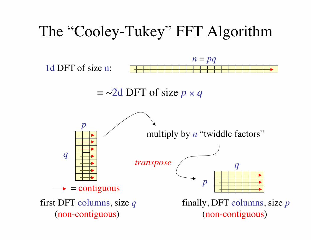
The “Cooley-Tukey” FFT Algorithm
1d DFT of size n:n = pq
= ~2d DFT of size p × q
first DFT columns, size q(non-contiguous)
multiply by n “twiddle factors”
q
p
transpose
finally, DFT columns, size p(non-contiguous)
p
q
= contiguous

“Cooley-Tukey” FFT, in math
twiddlessize-p DFTs size-q DFTs

…but how do we make it faster?
We (probably) cannot do better than Θ(n log n).(the proof of this remains an open problem)
[ unless we give up exactness ]
We’re left with the “constant” factor…
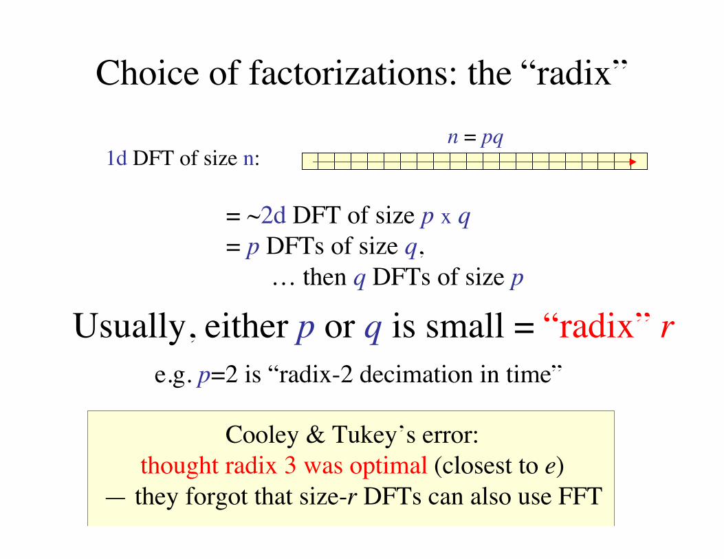
Choice of factorizations: the “radix”
1d DFT of size n:n = pq
= ~2d DFT of size p x q= p DFTs of size q, … then q DFTs of size p
Usually, either p or q is small = “radix” re.g. p=2 is “radix-2 decimation in time”
Cooley & Tukey’s error:thought radix 3 was optimal (closest to e)
— they forgot that size-r DFTs can also use FFT

The Next 30 Years…Assume “time” = # multiplications # multiplications + # additions (= flops)
Winograd (1979): # multiplications = Θ(n)(…realizable bound! … but costs too many additions)
Yavne (1968): split-radix FFT, saves 20% over radix-2 flops[ unsurpassed until last 2007, another ~6% saved
by Lundy/Van Buskirk and Johnson/Frigo ]

Are arithmetic counts so important?

The Next 30 Years…Assume “time” = # multiplications # multiplications + # additions (= flops)
Winograd (1979): # multiplications = Θ(n)(…realizable bound! … but costs too many additions)
Yavne (1968): split-radix FFT, saves 20% over radix-2 flops[ unsurpassed until last 2007, another ~6% saved]
last 15+ years: flop count (varies by ~20%)no longer determines speed (varies by factor of ~10+)

a basic question:
If arithmetic no longer dominates,what does?

The Memory Hierarchy (not to scale)
disk (out of core) / remote memory (parallel)(terabytes)
L2 cache (megabytes)
L1 cache (10s of kilobytes)
registers (~100)
RAM (gigabytes)
the name of the game:• do as much work as possible before going out of cache
…what matters is nothow much work youdo, but when and whereyou do it.
…difficult for FFTs…many complications…continually changing

What’s the fastest algorithm for _____?(computer science = math + time = math + $)
1
3
Find best asymptotic complexitynaïve DFT to FFT: O(n2) to O(n log n)
Find variant/implementation that runs fastesthardware-dependent — unstable answer!
2 Find best exact operation count?
Better to change the question…

What’s the smallestset of “simple” algorithmic steps
whose compositions ~alwaysspan the ~fastest algorithm?
A question with a more stable answer?

FFTW
• C library for real & complex FFTs (arbitrary size/dimensionality)
• Computational kernels (80% of code) automatically generated
• Self-optimizes for your hardware (picks best composition of steps)= portability + performance
(+ parallel versions for threads & MPI)
free software: http://www.fftw.org/
the “FastestFourier Tranform
in the West”

FFTW performancepower-of-two sizes, double precision
833 MHz Alpha EV6 2 GHz PowerPC G5
2 GHz AMD Opteron 500 MHz Ultrasparc IIe

FFTW performancenon-power-of-two sizes, double precision
833 MHz Alpha EV6
2 GHz AMD Opteron
unusual: non-power-of-two sizesreceive as much optimization
as powers of two
…because welet the code do the optimizing
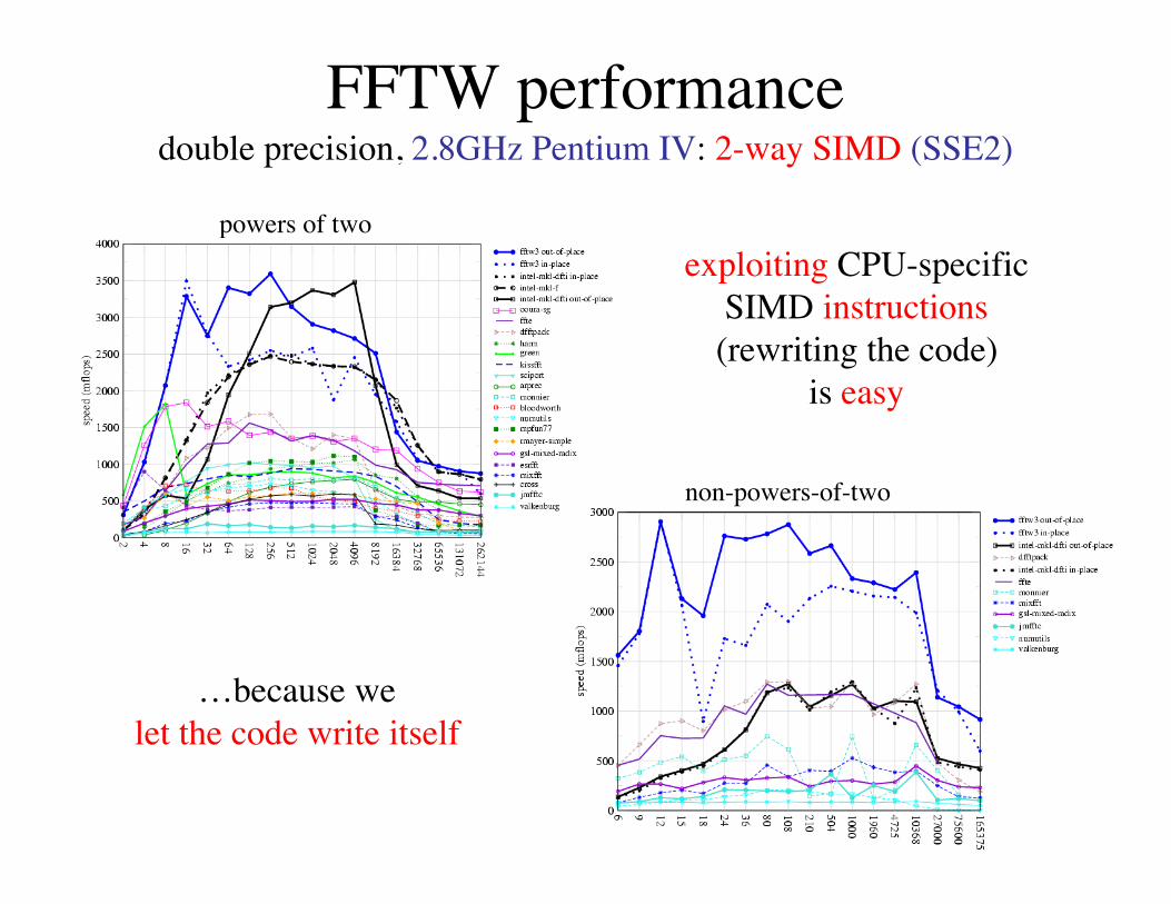
FFTW performancedouble precision, 2.8GHz Pentium IV: 2-way SIMD (SSE2)
powers of two
…because welet the code write itself
non-powers-of-two
exploiting CPU-specificSIMD instructions(rewriting the code)
is easy

Why is FFTW fast?FFTW implements many FFT algorithms:
A planner picks the best composition (plan)by measuring the speed of different combinations.
A recursive framework enhances locality.
3
1
2
Three ideas:
Computational kernels (codelets)should be automatically generated.
Determining the unit of composition is critical.

FFTW is easy to use{
complex x[n];plan p;
p = plan_dft_1d(n, x, x, FORWARD, MEASURE);...execute(p); /* repeat as needed */...destroy_plan(p);
}
Key fact: usually,many transforms of same size
are required.

Why is FFTW fast?FFTW implements many FFT algorithms:
A planner picks the best composition (plan)by measuring the speed of different combinations.
A recursive framework enhances locality.
3
1
2
Three ideas:
Computational kernels (codelets)should be automatically generated.
Determining the unit of composition is critical.

Why is FFTW slow?1965 Cooley & Tukey, IBM 7094, 36-bit single precision:
size 2048 DFT in 1.2 seconds2003 FFTW3+SIMD, 2GHz Pentium-IV 64-bit double precision:
size 2048 DFT in 50 microseconds (24,000x speedup)(= 30% improvement per year)
(= doubles every ~30 months)
don’t get “peak” CPU speedespecially for large n,
unlike e.g. dense matrix multiply
FFTs are hard:
Moore’s prediction:30 nanoseconds( )
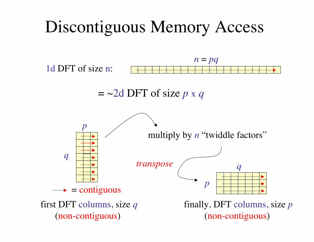
Discontiguous Memory Access
1d DFT of size n:n = pq
= ~2d DFT of size p x q
first DFT columns, size q(non-contiguous)
multiply by n “twiddle factors”
q
p
transpose
finally, DFT columns, size p(non-contiguous)
p
q
= contiguous

But traditional implementation is non-recursive,breadth-first traversal:
log2 n passes over whole array
Cooley-Tukey is NaturallyRecursive
Size 8 DFT
Size 4 DFT Size 4 DFT
Size 2 DFT Size 2 DFT Size 2 DFT Size 2 DFT
p = 2 (radix 2)

breadth-first, but with blocks of size = cacheoptimal choice: radix = cache size
radix >> 2
Traditional cache solution: Blocking
Size 8 DFT
Size 4 DFT Size 4 DFT
Size 2 DFT Size 2 DFT Size 2 DFT Size 2 DFT
p = 2 (radix 2)
…requires program specialized for cache size…multiple levels of cache = multilevel blocking

Recursive Divide & Conquer is Good
Size 8 DFT
Size 4 DFT Size 4 DFT
Size 2 DFT Size 2 DFT Size 2 DFT Size 2 DFT
p = 2 (radix 2)
eventually small enough to fit in cache…no matter what size the cache is
(depth-first traversal) [Singleton, 1967]

Cache Obliviousness• A cache-oblivious algorithm does not know the cache size
— for many algorithms [Frigo 1999], can be provably “big-O” optimal for any machine
& for all levels of cache simultaneously
… but this ignores e.g. constant factors, associativity, …
cache-obliviousness is a good beginning,but is not the end of optimization
we’ll see: FFTW combines both styles(breadth- and depth-first) with self-optimization

Why is FFTW fast?FFTW implements many FFT algorithms:
A planner picks the best composition (plan)by measuring the speed of different combinations.
A recursive framework enhances locality.
3
1
2
Three ideas:
Computational kernels (codelets)should be automatically generated.
Determining the unit of composition is critical.

The Codelet Generator
• Generates fast hard-coded C for FFT of a given size
a domain-specific FFT “compiler”
Necessary to give the planner alarge space of codelets to
experiment with (anyfactorization).
Exploits modern CPUdeep pipelines & large register sets.
Allows easy experimentation withdifferent optimizations & algorithms.
…CPU-specific hacks (SIMD) feasible
(& negates recursion overhead)
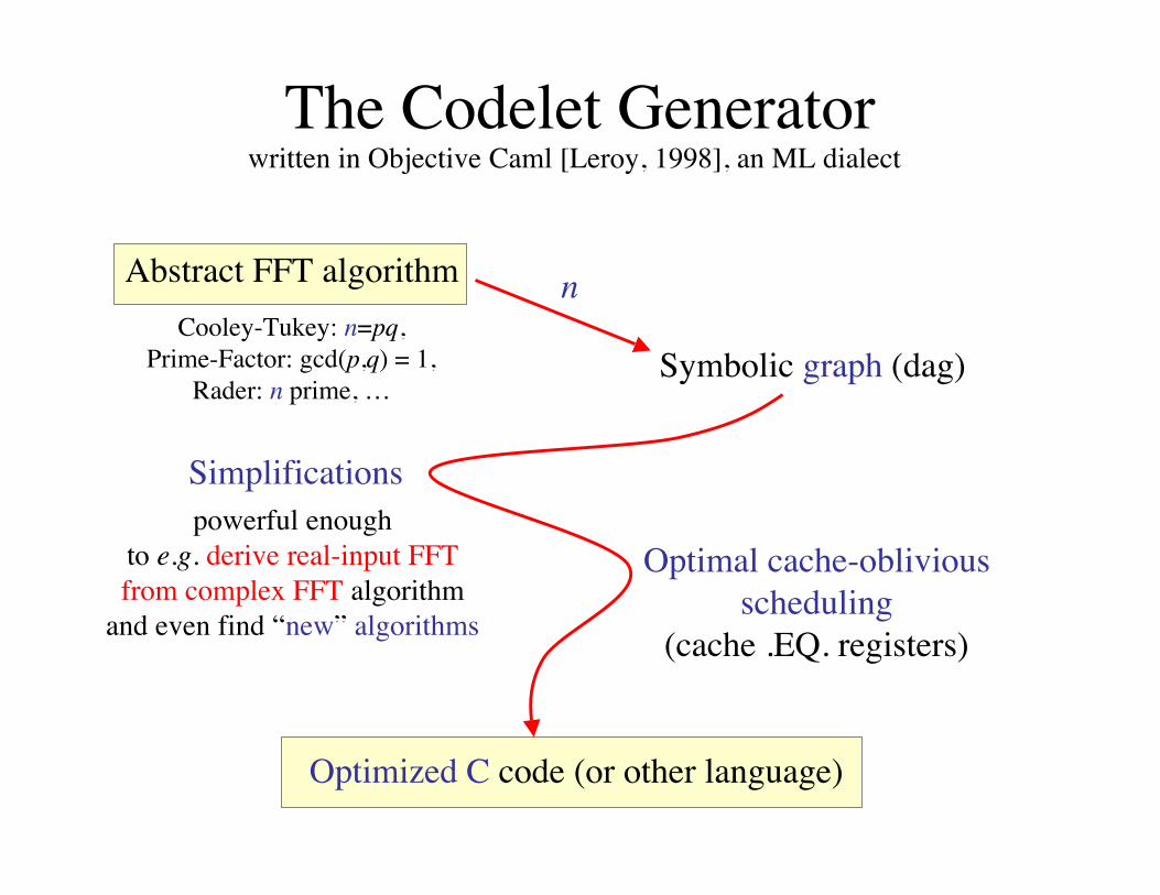
The Codelet Generator
Symbolic graph (dag)
Simplifications
Optimal cache-obliviousscheduling
(cache .EQ. registers)
Optimized C code (or other language)
written in Objective Caml [Leroy, 1998], an ML dialect
n
powerful enoughto e.g. derive real-input FFTfrom complex FFT algorithm
and even find “new” algorithms
Abstract FFT algorithmCooley-Tukey: n=pq,
Prime-Factor: gcd(p,q) = 1,Rader: n prime, …

The Generator Finds Good/New FFTs

Symbolic Algorithms are EasyCooley-Tukey in OCaml

Simple Simplifications
Well-known optimizations:
Algebraic simplification, e.g. a + 0 = a
Constant folding
Common-subexpression elimination

Symbolic Pattern Matching in OCaml
stimesM = function | (Uminus a, b) -> stimesM (a, b) >>= suminusM | (a, Uminus b) -> stimesM (a, b) >>= suminusM | (Num a, Num b) -> snumM (Number.mul a b) | (Num a, Times (Num b, c)) -> snumM (Number.mul a b) >>= fun x -> stimesM (x, c) | (Num a, b) when Number.is_zero a -> snumM Number.zero | (Num a, b) when Number.is_one a -> makeNode b | (Num a, b) when Number.is_mone a -> suminusM b | (a, b) when is_known_constant b && not (is_known_constant a) -> stimesM (b, a) | (a, b) -> makeNode (Times (a, b))
The following actual code fragment issolely responsible for simplifying multiplications:
(Common-subexpression elimination is implicit via “memoization” and monadic programming style.)

Simple Simplifications
Well-known optimizations:
Algebraic simplification, e.g. a + 0 = a
Constant folding
Common-subexpression elimination
FFT-specific optimizations:
_________________ negative constants…
Network transposition (transpose + simplify + transpose)

A Quiz: Is One Faster?
a = 0.5 * b;c = 0.5 * d;e = 1.0 + a;f = 1.0 - c;
a = 0.5 * b;c = -0.5 * d;e = 1.0 + a;f = 1.0 + c;
Both compute the same thing, andhave the same number of arithmetic operations:
Faster because noseparate load for -0.5
10–15% speedup

Non-obvious transformationsrequire experimentation

Quiz 2: Which is Faster?
array[stride * i] array[strides[i]]
strides[i] = stride * iusing precomputed stride array:
accessing strided arrayinside codelet (amid dense numeric code), nonsequential
…namely, Intel Pentia:integer multiplication
conflicts with floating-point
This is faster, of course!Except on brain-dead architectures…
up to ~10–20% speedup
(even better to bloat: pregenerate various constant strides)

Machine-specific hacksare feasible
if you just generate special code
stride precomputation
SIMD instructions (SSE, Altivec, 3dNow!)
fused multiply-add instructions…
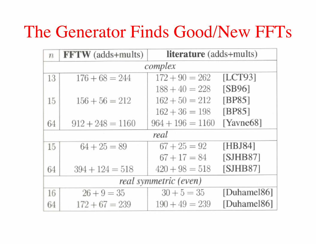
The Generator Finds Good/New FFTs

Why is FFTW fast?FFTW implements many FFT algorithms:
A planner picks the best composition (plan)by measuring the speed of different combinations.
A recursive framework enhances locality.
3
1
2
Three ideas:
Computational kernels (codelets)should be automatically generated.
Determining the unit of composition is critical.

What does the planner compose?• The Cooley-Tukey algorithm presents many choices:
— which factorization? what order? memory reshuffling?
FFTW 1 (1997):
Find simple steps that combine without restrictionto form many different algorithms.
steps solve out-of-place DFT of size n
… steps to do WHAT?

“Composable” Steps in FFTW 1
SOLVE — Directly solve a small DFT by a codelet
CT-FACTOR[r] — Radix-r Cooley-Tukey step = execute loop of r sub-problems of size n/r
Many algorithms difficult to express via simple steps.
— e.g. expresses only depth-first recursion(loop is outside of sub-problem)
— e.g. in-place without bit-reversalrequires combining
two CT steps (DIT + DIF) + transpose

What does the planner compose?• The Cooley-Tukey algorithm presents many choices:
— which factorization? what order? memory reshuffling?
FFTW 1 (1997):
Find simple steps that combine without restrictionto form many different algorithms.
steps solve out-of-place DFT of size n
… steps to do WHAT?
Steps cannot solve problems that cannot be expressed.
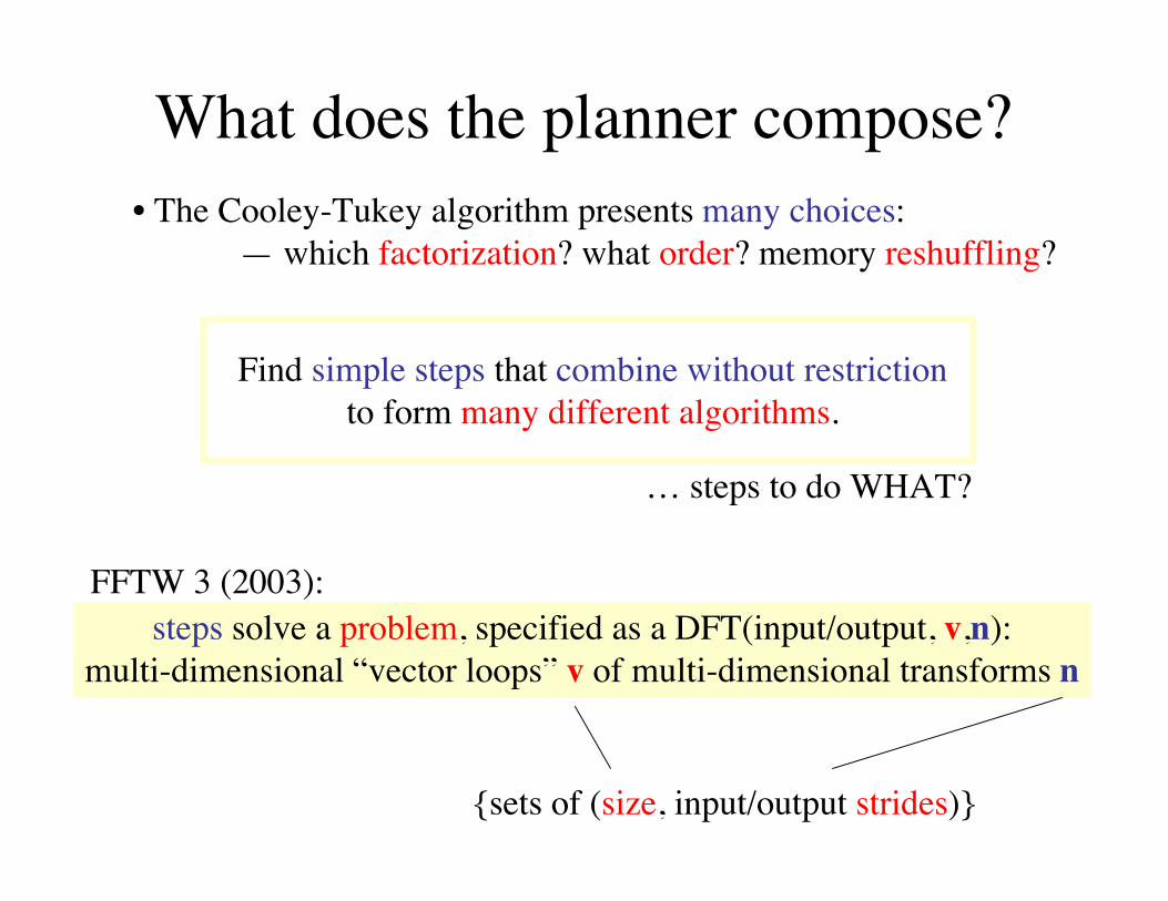
What does the planner compose?• The Cooley-Tukey algorithm presents many choices:
— which factorization? what order? memory reshuffling?
FFTW 3 (2003):
Find simple steps that combine without restrictionto form many different algorithms.
steps solve a problem, specified as a DFT(input/output, v,n):multi-dimensional “vector loops” v of multi-dimensional transforms n
{sets of (size, input/output strides)}
… steps to do WHAT?
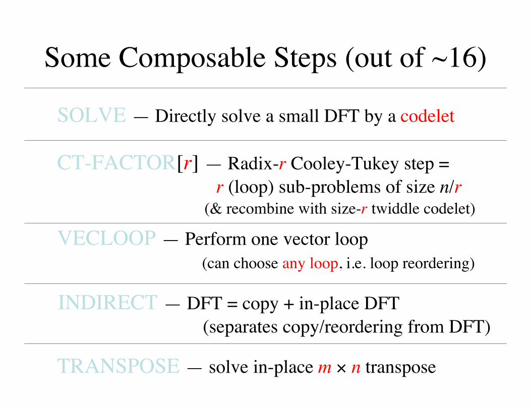
Some Composable Steps (out of ~16)
SOLVE — Directly solve a small DFT by a codelet
CT-FACTOR[r] — Radix-r Cooley-Tukey step = r (loop) sub-problems of size n/r
VECLOOP — Perform one vector loop(can choose any loop, i.e. loop reordering)
INDIRECT — DFT = copy + in-place DFT(separates copy/reordering from DFT)
TRANSPOSE — solve in-place m × n transpose
(& recombine with size-r twiddle codelet)

Many Resulting “Algorithms”• INDIRECT + TRANSPOSE gives in-place DFTs,
— bit-reversal = product of transpositions… no separate bit-reversal “pass”
[ Johnson (unrelated) & Burrus (1984) ]
• CT-FACTOR then VECLOOP(s) gives “breadth-first” FFT,— erases iterative/recursive distinction
• VECLOOP can push topmost loop to “leaves”— “vector” FFT algorithm [ Swarztrauber (1987) ]
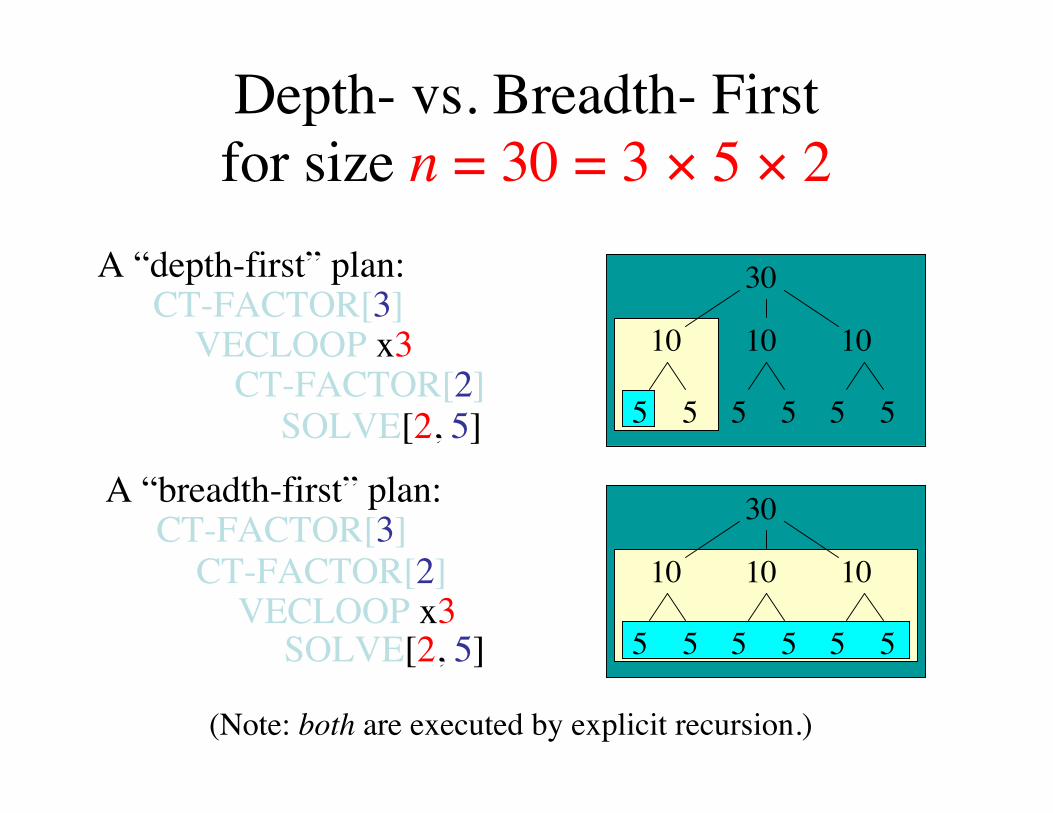
Depth- vs. Breadth- Firstfor size n = 30 = 3 × 5 × 2
A “depth-first” plan:CT-FACTOR[3]
VECLOOP x3CT-FACTOR[2]
SOLVE[2, 5]
CT-FACTOR[3]
VECLOOP x3CT-FACTOR[2]
SOLVE[2, 5]
A “breadth-first” plan:
(Note: both are executed by explicit recursion.)
30
10 10 10
5 5 5 5 5 5
30
10 10 10
5 5 5 5 5 5

Many Resulting “Algorithms”• INDIRECT + TRANSPOSE gives in-place DFTs,
— bit-reversal = product of transpositions… no separate bit-reversal “pass”
[ Johnson (unrelated) & Burrus (1984) ]
• CT-FACTOR then VECLOOP(s) gives “breadth-first” FFT,— erases iterative/recursive distinction
• VECLOOP can push topmost loop to “leaves”— “vector” FFT algorithm [ Swarztrauber (1987) ]

In-place plan for size 214 = 16384(2 GHz PowerPC G5, double precision)
CT-FACTOR[32]CT-FACTOR[16]
INDIRECT
SOLVE[512, 32]TRANSPOSE[32 × 32] x16
Radix-32 DIT + Radix-32 DIF = 2 loops = transpose… where leaf SOLVE ~ “radix” 32 x 1

Out-of-place plan for size 219=524288(2GHz Pentium IV, double precision)
CT-FACTOR[4] (buffered variant)CT-FACTOR[32] (buffered variant)
VECLOOP (reorder) x32CT-FACTOR[64]
INDIRECT
VECLOOP x4SOLVE[64, 64]
VECLOOP (reorder) x64VECLOOP x4
COPY[64]
Unpredictable: (automated) experimentation is the only solution.
INDIRECT+
VECLOOP (reorder)(+ …)
=huge improvements
for large 1d sizes
~2000 lineshard-coded C!
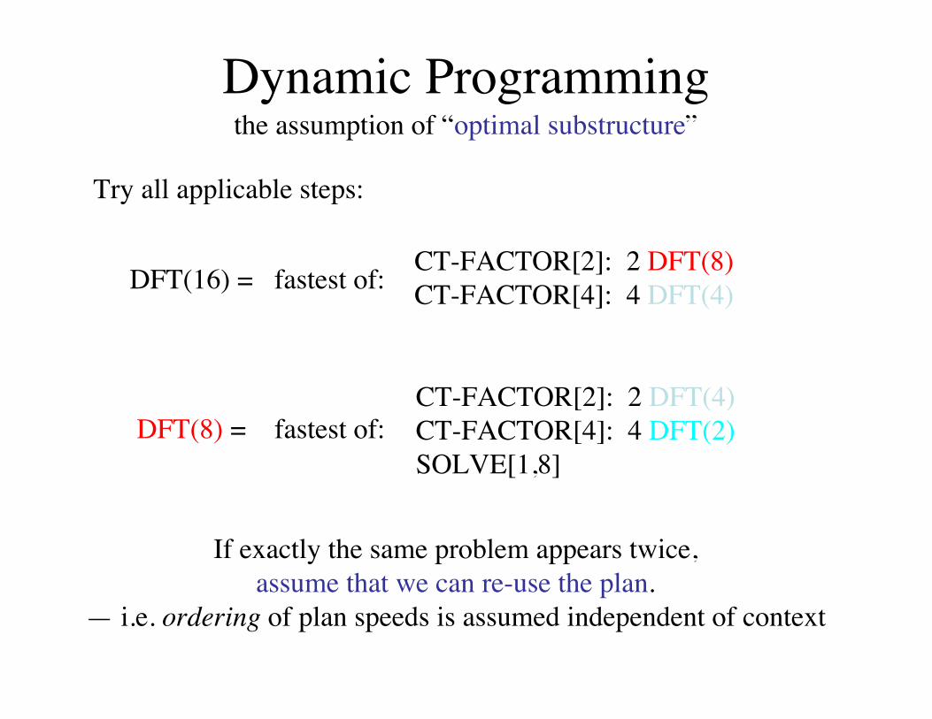
Dynamic Programmingthe assumption of “optimal substructure”
DFT(16) = fastest of: CT-FACTOR[2]: 2 DFT(8)CT-FACTOR[4]: 4 DFT(4)
DFT(8) = fastest of:CT-FACTOR[2]: 2 DFT(4)CT-FACTOR[4]: 4 DFT(2)SOLVE[1,8]
Try all applicable steps:
If exactly the same problem appears twice,assume that we can re-use the plan.
— i.e. ordering of plan speeds is assumed independent of context

Planner Unpredictabilitydouble-precision, power-of-two sizes, 2GHz PowerPC G5
FFTW 3
heuristic: pick planwith fewest
adds + multiplies + loads/stores
Classic strategy:minimize op’s
fails badly
Use plan from:another machine?e.g. Pentium-IV?… lose 20–40%
another test:

We’ve Come a Long Way?In the name of performance, computers have become complex & unpredictable.
•
Optimization is hard: simple heuristics (e.g. fewest flops) no longer work.
•
One solution is to avoid the details, not embrace them:(Recursive) composition of simple modules
+ feedback (self-optimization)High-level languages (not C) & code generation are a powerful tool for high performance.
•