fastest fourier transform in the west · fastest fourier transform in the west devendra ghate and...
TRANSCRIPT
Fastest Fourier Transform in theWest
Devendra Ghate and Nachi Gupta
[email protected], [email protected]
Oxford University Computing Laboratory
MT 2006 Internal Seminar – p. 1/33
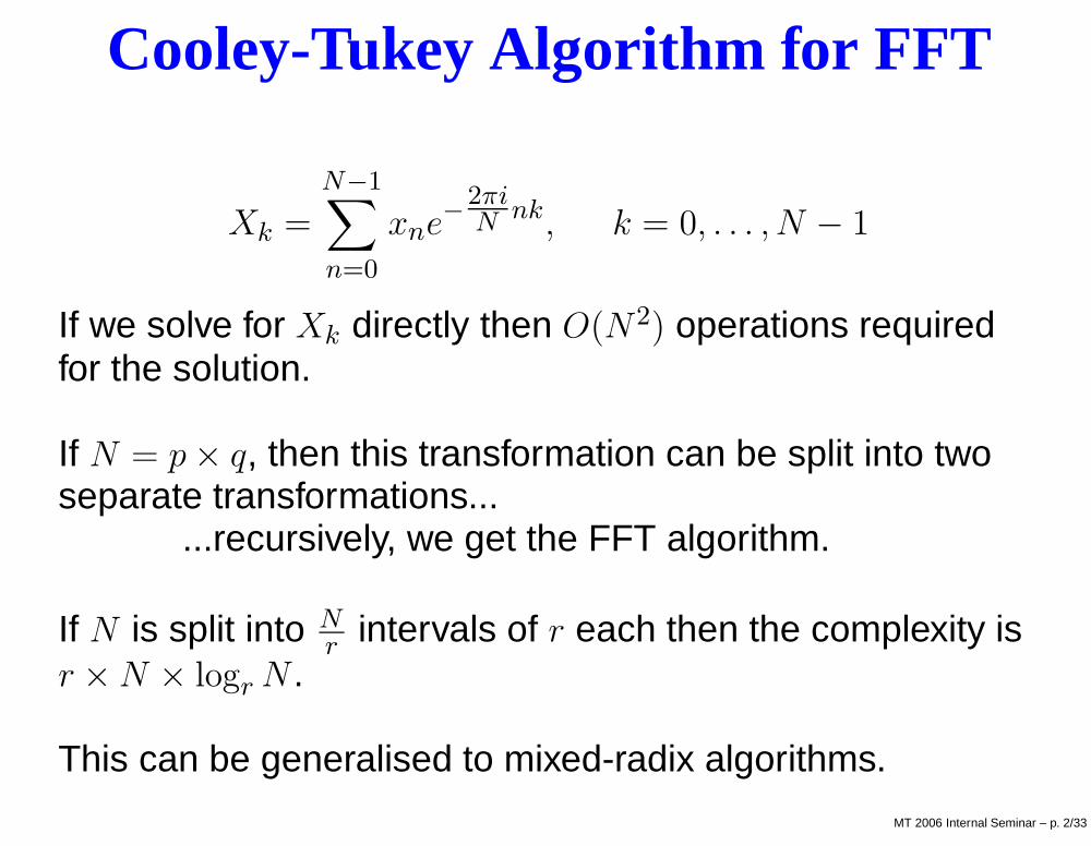
Cooley-Tukey Algorithm for FFT
Xk =N−1∑
n=0
xne−2πi
Nnk, k = 0, . . . , N − 1
If we solve for Xk directly then O(N2) operations requiredfor the solution.
If N = p × q, then this transformation can be split into twoseparate transformations...
...recursively, we get the FFT algorithm.
If N is split into N
rintervals of r each then the complexity is
r × N × logr N .
This can be generalised to mixed-radix algorithms.
MT 2006 Internal Seminar – p. 2/33
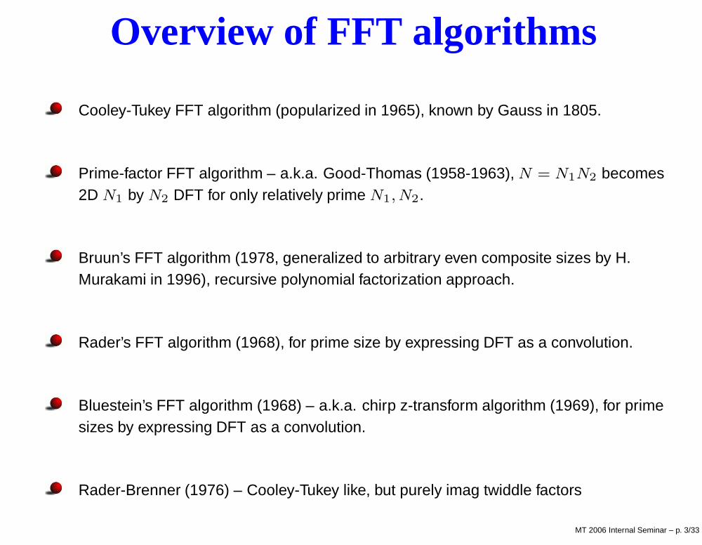
Overview of FFT algorithms
Cooley-Tukey FFT algorithm (popularized in 1965), known by Gauss in 1805.
Prime-factor FFT algorithm – a.k.a. Good-Thomas (1958-1963), N = N1N2 becomes2D N1 by N2 DFT for only relatively prime N1, N2.
Bruun’s FFT algorithm (1978, generalized to arbitrary even composite sizes by H.Murakami in 1996), recursive polynomial factorization approach.
Rader’s FFT algorithm (1968), for prime size by expressing DFT as a convolution.
Bluestein’s FFT algorithm (1968) – a.k.a. chirp z-transform algorithm (1969), for primesizes by expressing DFT as a convolution.
Rader-Brenner (1976) – Cooley-Tukey like, but purely imag twiddle factors
MT 2006 Internal Seminar – p. 3/33
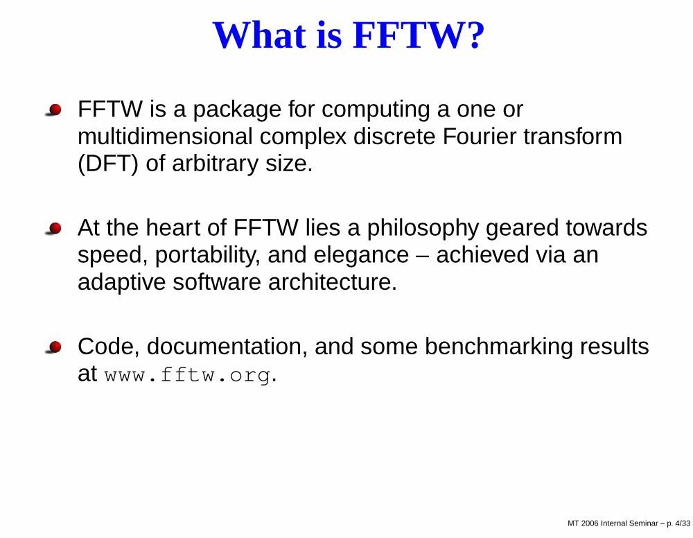
What is FFTW?
FFTW is a package for computing a one ormultidimensional complex discrete Fourier transform(DFT) of arbitrary size.
At the heart of FFTW lies a philosophy geared towardsspeed, portability, and elegance – achieved via anadaptive software architecture.
Code, documentation, and some benchmarking resultsat www.fftw.org.
MT 2006 Internal Seminar – p. 4/33
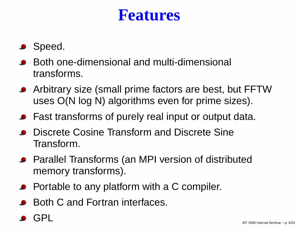
Features
Speed.
Both one-dimensional and multi-dimensionaltransforms.
Arbitrary size (small prime factors are best, but FFTWuses O(N log N) algorithms even for prime sizes).
Fast transforms of purely real input or output data.
Discrete Cosine Transform and Discrete SineTransform.
Parallel Transforms (an MPI version of distributedmemory transforms).
Portable to any platform with a C compiler.
Both C and Fortran interfaces.
GPLMT 2006 Internal Seminar – p. 5/33
Wilkinson Prize
FFTW received the 1999 J. H. Wilkinson Prize forNumerical Software, which is awarded every four years tothe software that “best addresses all phases of thepreparation of high quality numerical software.”
Wilkinson, a seminal figure in modern numerical analysis,was a key proponent of the notion of reusable commonlibraries for scientific computing.
MT 2006 Internal Seminar – p. 6/33
Why FFTW is fast!
The transform is computed by an executor, composed ofhighly optimized composable blocks of C code calledcodelets.
At runtime, a planner finds an efficient way to mix thesecodelets: it measures the speeds of different plans andchooses the best using a dynamic programmingalgorithm.
The executor then interprets this plan with negligibleoverhead.
Codelets are generated automatically and fast.
MT 2006 Internal Seminar – p. 7/33
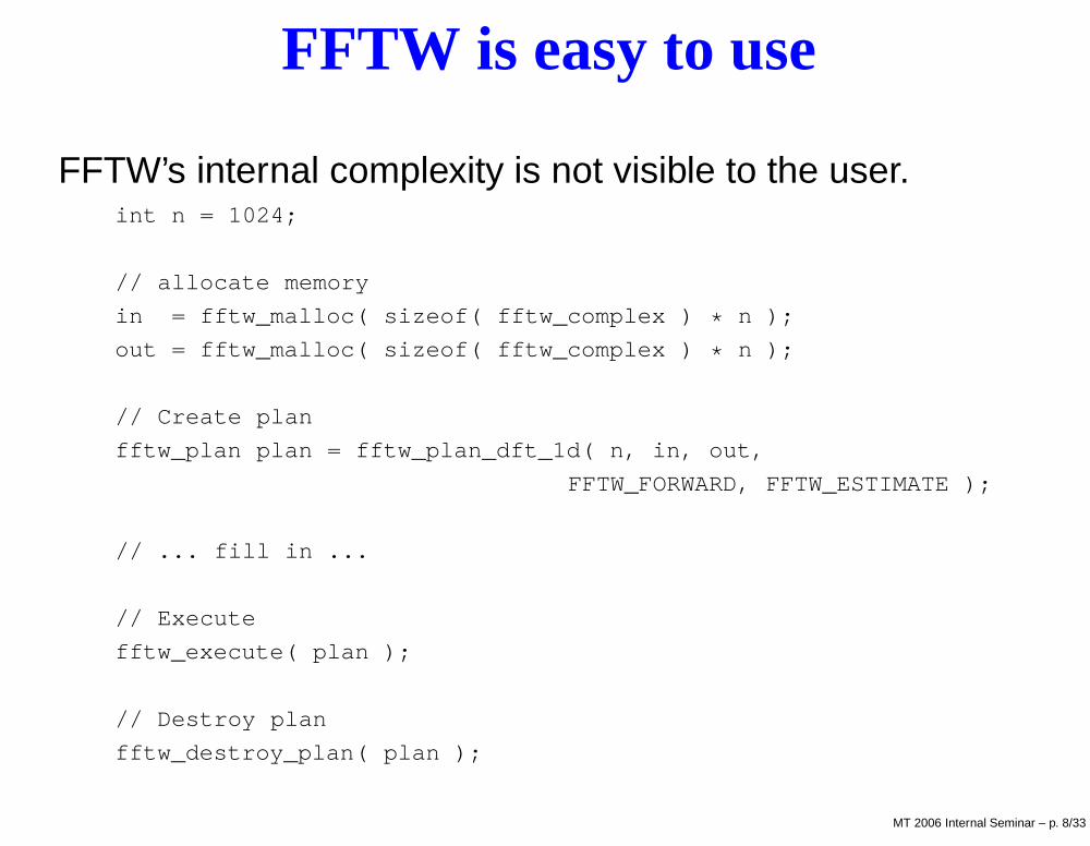
FFTW is easy to use
FFTW’s internal complexity is not visible to the user.int n = 1024;
// allocate memory
in = fftw_malloc( sizeof( fftw_complex ) * n );
out = fftw_malloc( sizeof( fftw_complex ) * n );
// Create plan
fftw_plan plan = fftw_plan_dft_1d( n, in, out,
FFTW_FORWARD, FFTW_ESTIMATE );
// ... fill in ...
// Execute
fftw_execute( plan );
// Destroy plan
fftw_destroy_plan( plan );
MT 2006 Internal Seminar – p. 8/33
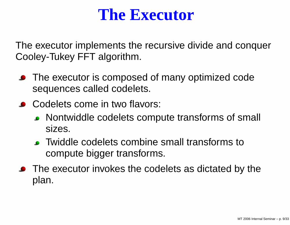
The Executor
The executor implements the recursive divide and conquerCooley-Tukey FFT algorithm.
The executor is composed of many optimized codesequences called codelets.
Codelets come in two flavors:Nontwiddle codelets compute transforms of smallsizes.Twiddle codelets combine small transforms tocompute bigger transforms.
The executor invokes the codelets as dictated by theplan.
MT 2006 Internal Seminar – p. 9/33
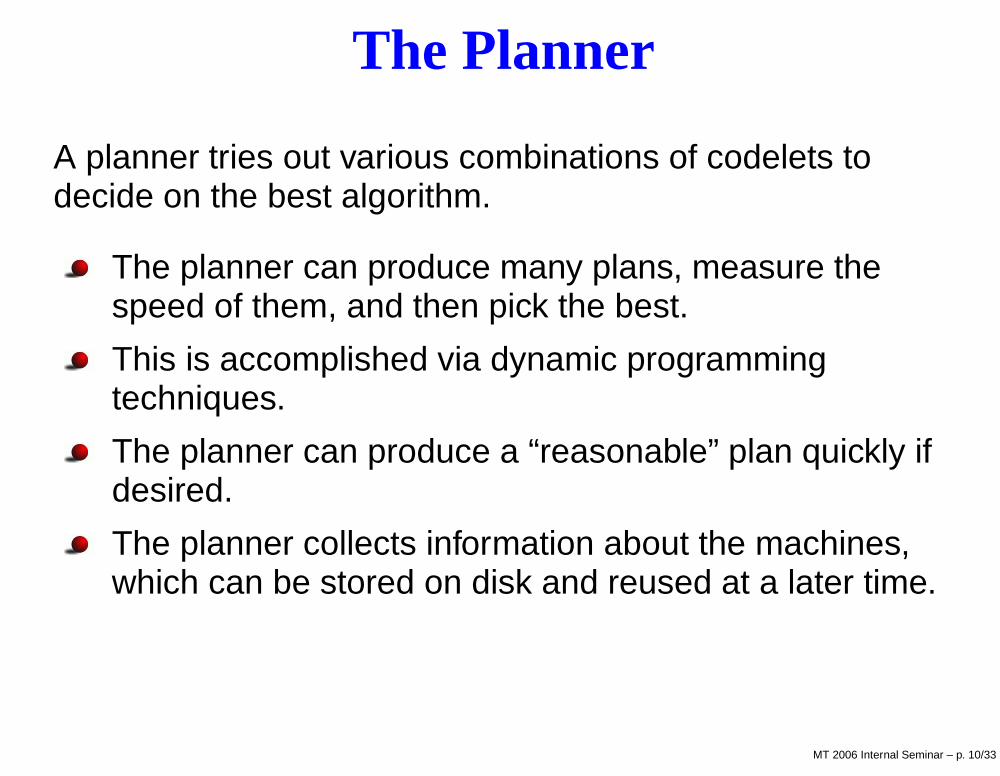
The Planner
A planner tries out various combinations of codelets todecide on the best algorithm.
The planner can produce many plans, measure thespeed of them, and then pick the best.
This is accomplished via dynamic programmingtechniques.
The planner can produce a “reasonable” plan quickly ifdesired.
The planner collects information about the machines,which can be stored on disk and reused at a later time.
MT 2006 Internal Seminar – p. 10/33
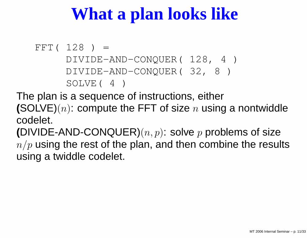
What a plan looks like
FFT( 128 ) =DIVIDE-AND-CONQUER( 128, 4 )DIVIDE-AND-CONQUER( 32, 8 )SOLVE( 4 )
The plan is a sequence of instructions, either(SOLVE)(n): compute the FFT of size n using a nontwiddlecodelet.(DIVIDE-AND-CONQUER)(n, p): solve p problems of sizen/p using the rest of the plan, and then combine the resultsusing a twiddle codelet.
MT 2006 Internal Seminar – p. 11/33
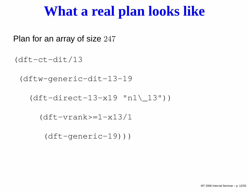
What a real plan looks like
Plan for an array of size 247
(dft-ct-dit/13
(dftw-generic-dit-13-19
(dft-direct-13-x19 "n1\_13"))
(dft-vrank>=1-x13/1
(dft-generic-19)))
MT 2006 Internal Seminar – p. 12/33
FFTW Plans
FFTW_ESTIMATE - no run-time tuning, probablysuboptimal
FFTW_MEASURE - experiment with differentalgorithms and choose fastest
FFTW_PATIENT - experiment with more algorithms, ...
FFTW_EXHAUSTIVE - even more, ...
Creating a plan for an array of size 823467 inFFTW_EXHAUSTIVE modes takes 25 minutes.
MT 2006 Internal Seminar – p. 13/33
Wisdom
A central or local database of plans for various array sizesfor a given hardware configuration.
Helps greatly in the estimate mode
Reduces computation time for the exhaustive mode
Wisdom from the other array sizes is also utilised
Can be exported from one architecture to another
Matlab uses a wisdom database by default.
MT 2006 Internal Seminar – p. 14/33
FFTW Compiler
Various basic algorithms written in CamL (a functionallanguage)
Directed acyclic graph (DAG) created for all thesealgorithms
Optimisation rules defined especially suited for FFTalgorithms (these also include standard optimisationscarried out by a compiler)
Small snippets of code, “codelets”, generated for FFTalgorithms of size N = 2 : 16
MT 2006 Internal Seminar – p. 15/33
Multi-dimensional Arrays
FFTW does not accept multidimensional arrays.
A single dimensional array in the "row-major" format (Cstandard)
Use of fftw_malloc for contiguous array allocation
MKL routines accept multi-dimensinal arrays. Variouscompact formats are also defined.
MT 2006 Internal Seminar – p. 16/33
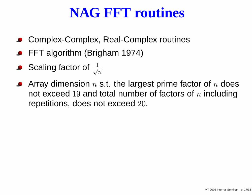
NAG FFT routines
Complex-Complex, Real-Complex routines
FFT algorithm (Brigham 1974)
Scaling factor of 1√
n
Array dimension n s.t. the largest prime factor of n doesnot exceed 19 and total number of factors of n includingrepetitions, does not exceed 20.
MT 2006 Internal Seminar – p. 17/33
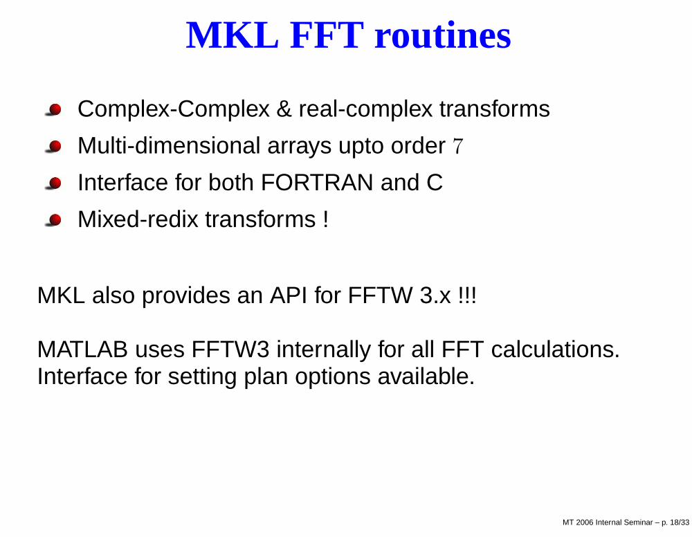
MKL FFT routines
Complex-Complex & real-complex transforms
Multi-dimensional arrays upto order 7
Interface for both FORTRAN and C
Mixed-redix transforms !
MKL also provides an API for FFTW 3.x !!!
MATLAB uses FFTW3 internally for all FFT calculations.Interface for setting plan options available.
MT 2006 Internal Seminar – p. 18/33
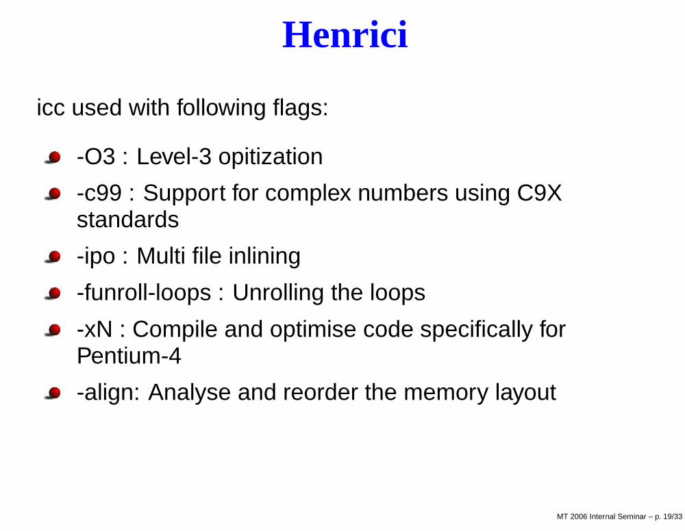
Henrici
icc used with following flags:
-O3 : Level-3 opitization
-c99 : Support for complex numbers using C9Xstandards
-ipo : Multi file inlining
-funroll-loops : Unrolling the loops
-xN : Compile and optimise code specifically forPentium-4
-align: Analyse and reorder the memory layout
MT 2006 Internal Seminar – p. 19/33
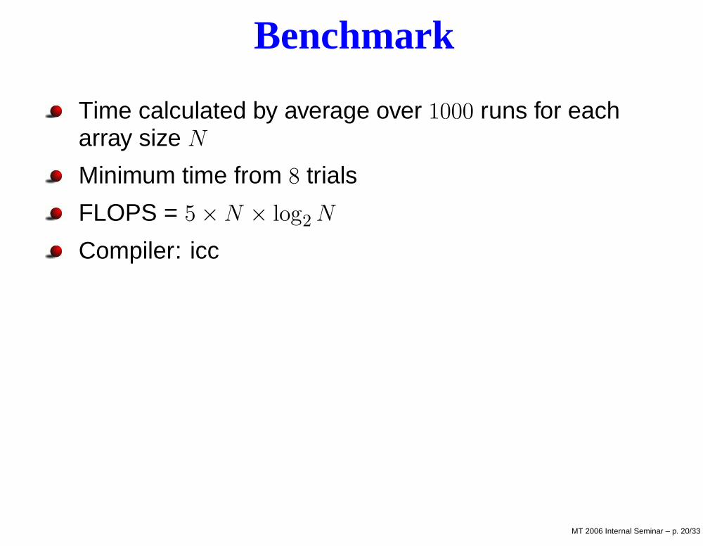
Benchmark
Time calculated by average over 1000 runs for eacharray size N
Minimum time from 8 trials
FLOPS = 5 × N × log2 N
Compiler: icc
MT 2006 Internal Seminar – p. 20/33
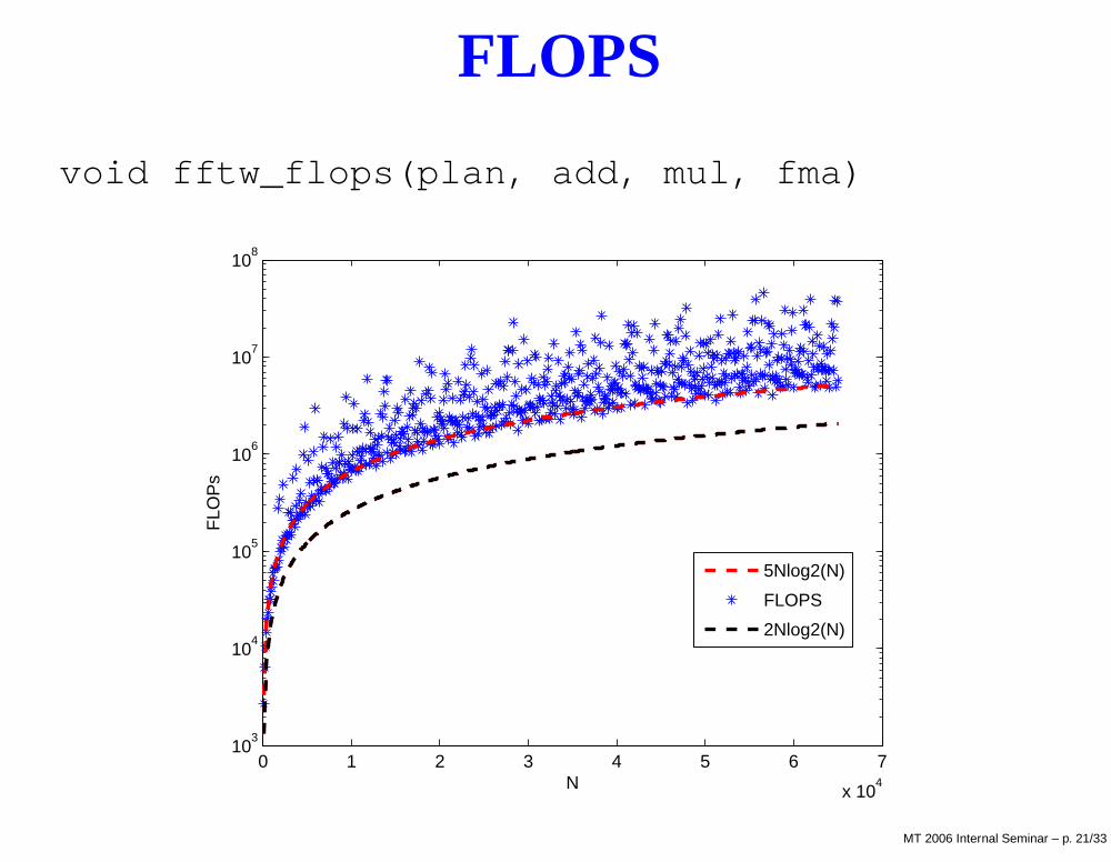
FLOPS
void fftw_flops(plan, add, mul, fma)
0 1 2 3 4 5 6 7
x 104
103
104
105
106
107
108
N
FLO
Ps
5Nlog2(N)
FLOPS
2Nlog2(N)
MT 2006 Internal Seminar – p. 21/33
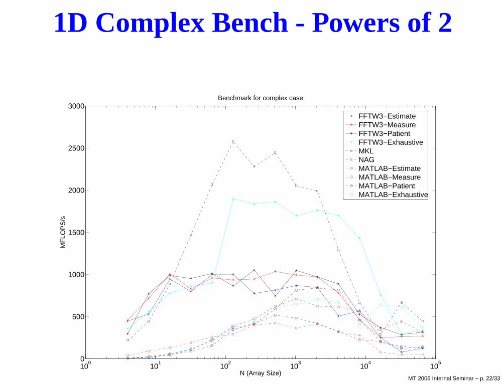
1D Complex Bench - Powers of 2
100
101
102
103
104
105
0
500
1000
1500
2000
2500
3000
N (Array Size)
MF
LOP
S/s
Benchmark for complex case
FFTW3−EstimateFFTW3−MeasureFFTW3−PatientFFTW3−ExhaustiveMKLNAGMATLAB−EstimateMATLAB−MeasureMATLAB−PatientMATLAB−Exhaustive
MT 2006 Internal Seminar – p. 22/33
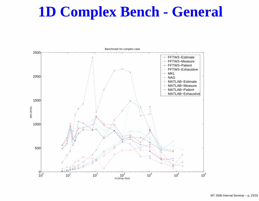
1D Complex Bench - General
100
101
102
103
104
105
106
0
500
1000
1500
2000
2500
N (Array Size)
MF
LOP
S/s
Benchmark for complex case
FFTW3−EstimateFFTW3−MeasureFFTW3−PatientFFTW3−ExhaustiveMKLNAGMATLAB−EstimateMATLAB−MeasureMATLAB−PatientMATLAB−Exhaustive
MT 2006 Internal Seminar – p. 23/33
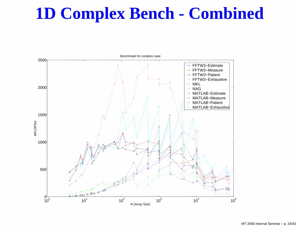
1D Complex Bench - Combined
100
101
102
103
104
105
0
500
1000
1500
2000
2500
N (Array Size)
MF
LOP
S/s
Benchmark for complex case
FFTW3−EstimateFFTW3−MeasureFFTW3−PatientFFTW3−ExhaustiveMKLNAGMATLAB−EstimateMATLAB−MeasureMATLAB−PatientMATLAB−Exhaustive
MT 2006 Internal Seminar – p. 24/33
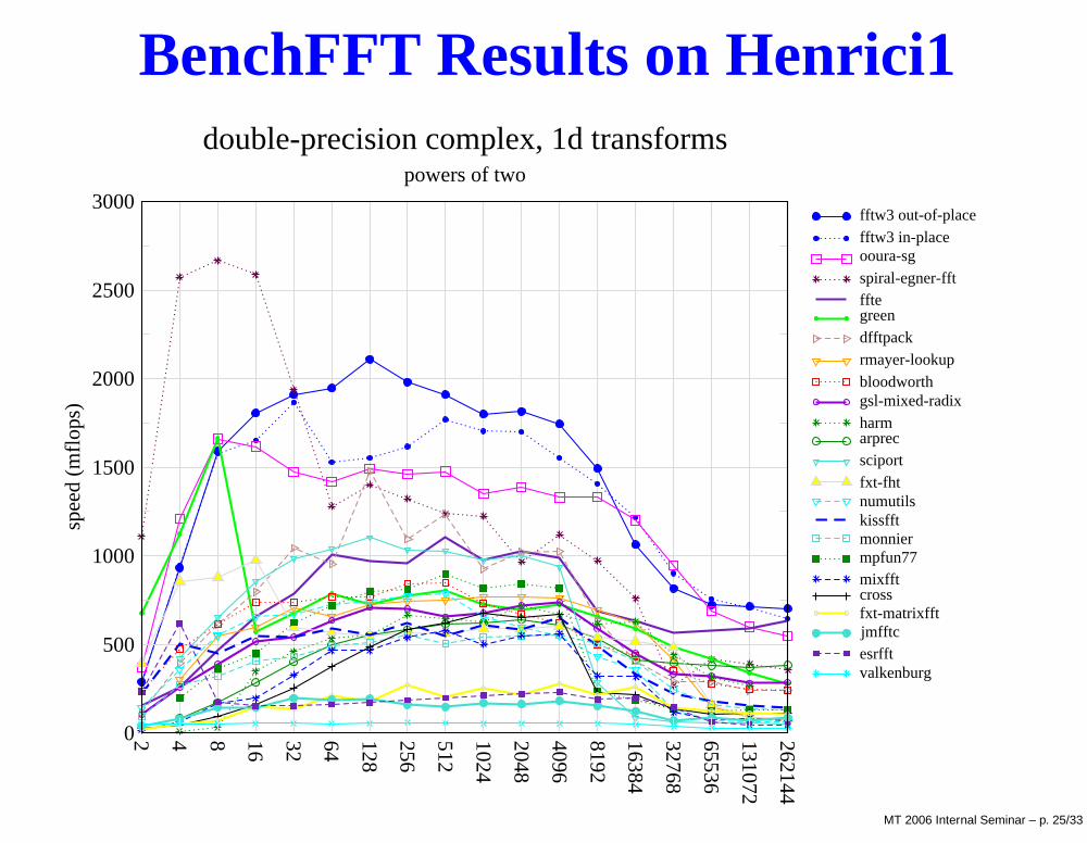
BenchFFT Results on Henrici1
2 4 8 16 32 64 128
256
512
1024
2048
4096
8192
16384
32768
65536
131072
262144
0
500
1000
1500
2000
2500
3000
spee
d (m
flop
s)
fftw3 out-of-placefftw3 in-placeooura-sg
spiral-egner-fftfftegreendfftpackrmayer-lookupbloodworthgsl-mixed-radixharmarprecsciportfxt-fhtnumutilskissfftmonniermpfun77mixfftcrossfxt-matrixfftjmfftcesrfftvalkenburg
double-precision complex, 1d transformspowers of two
MT 2006 Internal Seminar – p. 25/33
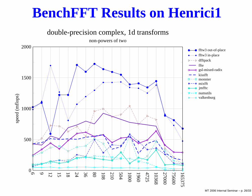
BenchFFT Results on Henrici1
6 9 12 15 18 24 36 80 108
210
504
1000
1960
4725
10368
27000
75600
165375
0
500
1000
1500
2000
spee
d (m
flop
s)
fftw3 out-of-placefftw3 in-placedfftpackfftegsl-mixed-radixkissfftmonniermixfftjmfftcnumutilsvalkenburg
double-precision complex, 1d transformsnon-powers of two
MT 2006 Internal Seminar – p. 26/33
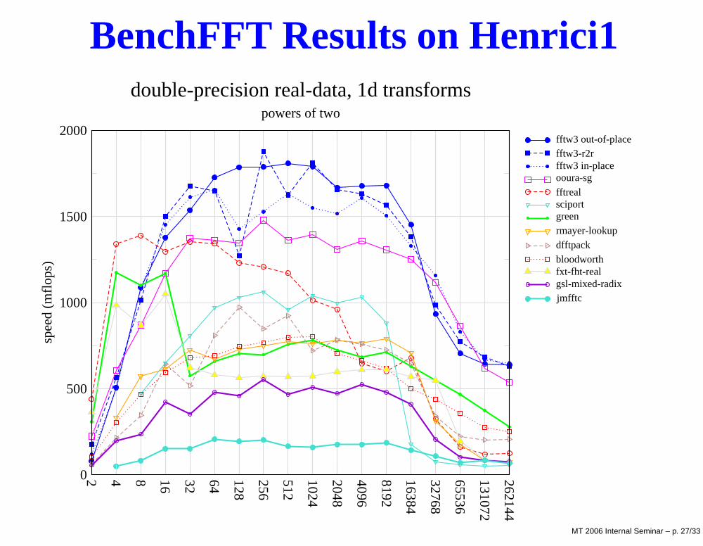
BenchFFT Results on Henrici1
2 4 8 16 32 64 128
256
512
1024
2048
4096
8192
16384
32768
65536
131072
262144
0
500
1000
1500
2000
spee
d (m
flop
s)
fftw3 out-of-placefftw3-r2rfftw3 in-placeooura-sg
fftrealsciportgreenrmayer-lookupdfftpackbloodworthfxt-fht-realgsl-mixed-radixjmfftc
double-precision real-data, 1d transformspowers of two
MT 2006 Internal Seminar – p. 27/33
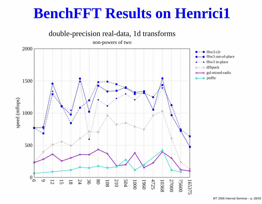
BenchFFT Results on Henrici1
6 9 12 15 18 24 36 80 108
210
504
1000
1960
4725
10368
27000
75600
165375
0
500
1000
1500
2000
spee
d (m
flop
s)
fftw3-r2rfftw3 out-of-placefftw3 in-place
dfftpackgsl-mixed-radixjmfftc
double-precision real-data, 1d transformsnon-powers of two
MT 2006 Internal Seminar – p. 28/33
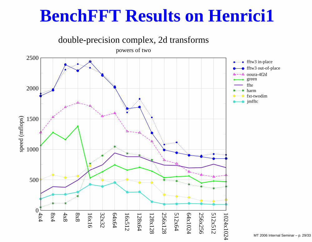
BenchFFT Results on Henrici1
4x4
8x4
4x8
8x8
16x16
32x32
64x64
16x512
128x64
128x128
256x128
512x64
64x1024
256x256
512x512
1024x1024
0
500
1000
1500
2000
2500
spee
d (m
flop
s)
fftw3 in-placefftw3 out-of-placeooura-4f2dgreenffteharmfxt-twodimjmfftc
double-precision complex, 2d transformspowers of two
MT 2006 Internal Seminar – p. 29/33
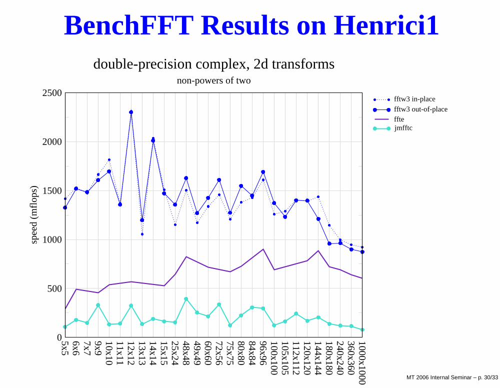
BenchFFT Results on Henrici1
5x56x67x79x910x1011x1112x1213x1314x1415x1525x2448x4849x4960x6072x5675x7580x8084x8496x96100x100105x105112x112120x120144x144180x180240x240360x3601000x1000
0
500
1000
1500
2000
2500
spee
d (m
flop
s)
fftw3 in-placefftw3 out-of-placefftejmfftc
double-precision complex, 2d transformsnon-powers of two
MT 2006 Internal Seminar – p. 30/33
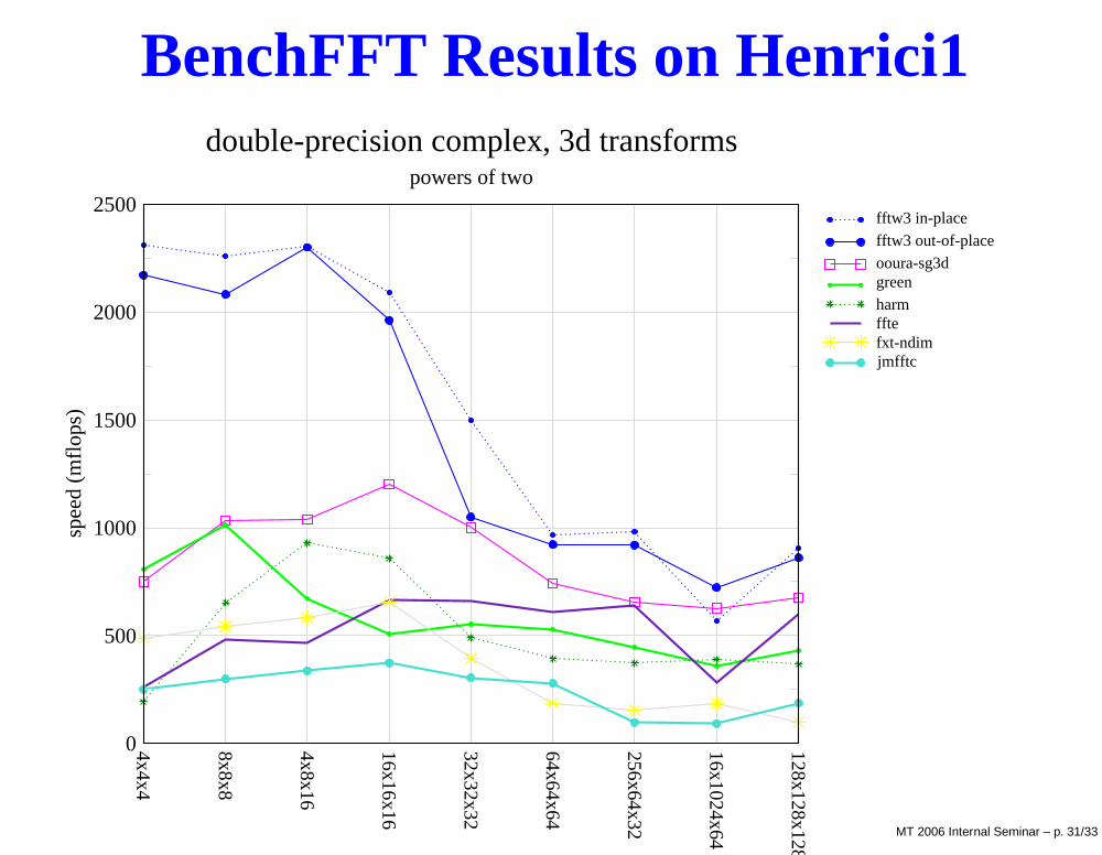
BenchFFT Results on Henrici1
4x4x4
8x8x8
4x8x16
16x16x16
32x32x32
64x64x64
256x64x32
16x1024x64
128x128x128
0
500
1000
1500
2000
2500
spee
d (m
flop
s)
fftw3 in-placefftw3 out-of-placeooura-sg3dgreenharmfftefxt-ndimjmfftc
double-precision complex, 3d transformspowers of two
MT 2006 Internal Seminar – p. 31/33
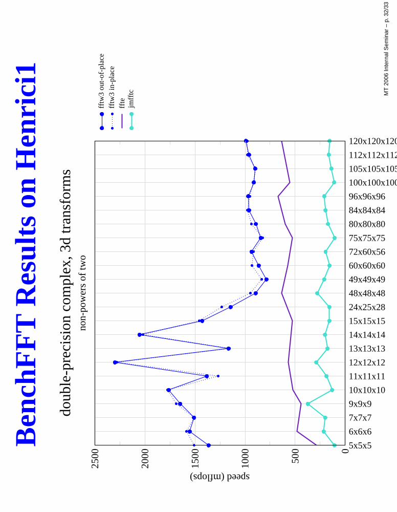
Ben
chF
FT
Res
ults
onH
enri
ci1
5x5x5
6x6x6
7x7x7
9x9x9
10x10x10
11x11x11
12x12x12
13x13x13
14x14x14
15x15x15
24x25x28
48x48x48
49x49x49
60x60x60
72x60x56
75x75x75
80x80x80
84x84x84
96x96x96
100x100x100
105x105x105
112x112x112
120x120x120
0
500
1000
1500
2000
2500
speed (mflops)
fftw
3 ou
t-of
-pla
ceff
tw3
in-p
lace
ffte
jmff
tc
doub
le-p
reci
sion
com
plex
, 3d
tran
sfor
ms
non-
pow
ers
of tw
o
MT
2006
Inte
rnal
Sem
inar
–p.
32/3
3
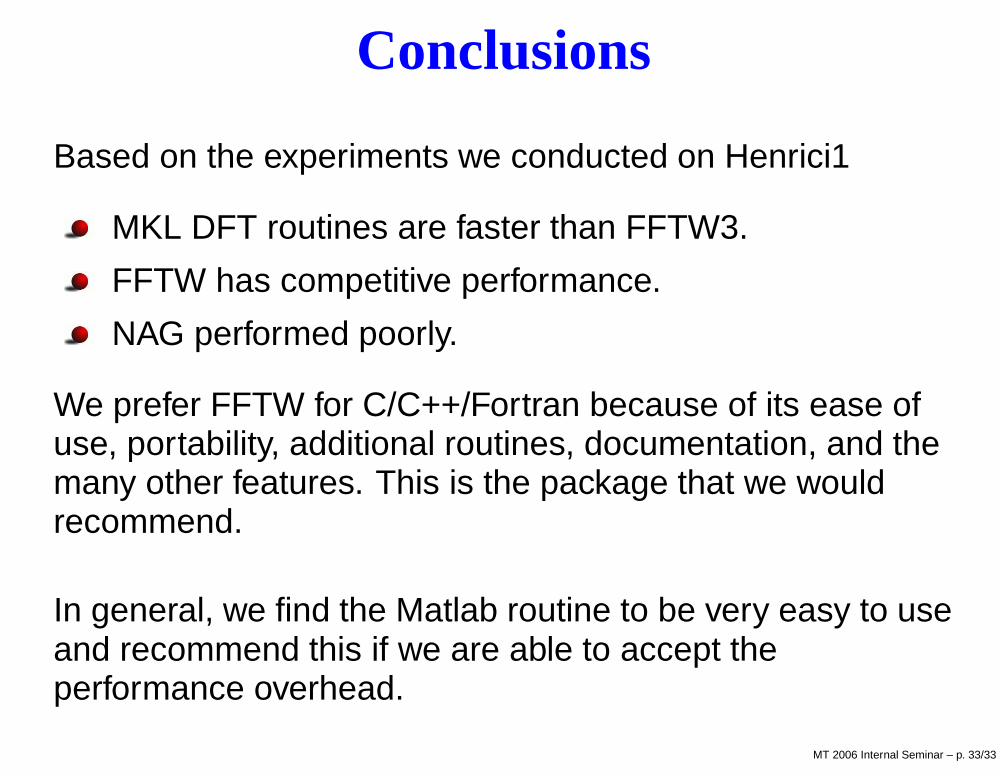
Conclusions
Based on the experiments we conducted on Henrici1
MKL DFT routines are faster than FFTW3.
FFTW has competitive performance.
NAG performed poorly.
We prefer FFTW for C/C++/Fortran because of its ease ofuse, portability, additional routines, documentation, and themany other features. This is the package that we wouldrecommend.
In general, we find the Matlab routine to be very easy to useand recommend this if we are able to accept theperformance overhead.
MT 2006 Internal Seminar – p. 33/33