arX

iv:a

stro

-ph/

0501

360v

1 1

7 Ja

n 20

05

The Evolution of Structure in X-ray Clusters of Galaxies

Tesla E. Jeltema1, Claude R. Canizares, Mark W. Bautz

Center for Space Research and Department of Physics

Massachusetts Institute of Technology

70 Vassar Street, Cambridge, MA 02139

tesla@ociw.edu

David A. Buote

Department of Physics and Astronomy

University of California at Irvine

4129 Frederick Reines Hall, Irvine, CA 92697

ABSTRACT

Using Chandra archival data, we quantify the evolution of cluster morphology

with redshift. Clusters form and grow through mergers with other clusters and

groups, and the amount of substructure in clusters in the present epoch and how

quickly it evolves with redshift depend on the underlying cosmology. Our sample

includes 40 X-ray selected, luminous clusters from the Chandra archive, and we

quantify cluster morphology using the power ratio method (Buote & Tsai 1995).

The power ratios are constructed from the moments of the X-ray surface bright-

ness and are related to a cluster’s dynamical state. We find that, as expected

qualitatively from hierarchical models of structure formation, high-redshift clus-

ters have more substructure and are dynamically more active than low-redshift

clusters. Specifically, the clusters with z > 0.5 have significantly higher aver-

age third and fourth order power ratios than the lower redshift clusters. Of the

power ratios, P3/P0 is the most unambiguous indicator of an asymmetric cluster

structure, and the difference in P3/P0 between the two samples remains signifi-

cant even when the effects of noise and other systematics are considered. After

correcting for noise, we apply a linear fit to P3/P0 versus redshift and find that

the slope is greater than zero at better than 99% confidence. This observation of

structure evolution indicates that dynamical state may be an important system-

atic effect in cluster studies seeking to constrain cosmology, and when calibrated

against numerical simulations, structure evolution will itself provide interesting

bounds on cosmological models.

– 2 –

Subject headings: galaxies: clusters: general — X-rays: galaxies:clusters — cos-

mology:observations

1. INTRODUCTION

Clusters form and grow through mergers with other clusters and groups. These mergers

are observed as multiple peaks in the cluster density distribution or as disturbed cluster

morphologies. The cluster relaxation time is relatively short, on the order of a Gyr, and the

fraction of unrelaxed clusters should reflect their formation rate. The formation epoch of

clusters depends on both Ωm and Λ, so the amount of substructure in clusters in the present

epoch and how quickly it evolves with redshift depend on these parameters. In low density

universes, clusters form earlier and will be on average more relaxed in the present epoch.

Clusters at high redshift, closer to the epoch of cluster formation, should be on average

dynamically younger and show more structure. In addition, mergers introduce systematic

errors in other cosmological studies with clusters. Mergers can lead to large deviations in

cluster luminosity, temperature, and velocity dispersion (Rowley, Thomas, & Kay 2004; Ran-

dall, Sarazin, & Ricker 2002; Mathiesen & Evrard 2001) and therefore errors in estimating

cluster mass and gas mass fraction as well as deviations from equilibrium. For these reasons,

a method of measuring cluster dynamical state and an understanding of how it evolves are

important.

A number of studies have been done on the structure of clusters at low-redshift. One of

the first systematic studies was conducted by Jones & Forman (1992) who visually examined

208 clusters observed with the Einstein X-ray satellite. They separated these clusters into

6 morphological classes including SINGLE, ELLIPTICAL, OFFSET CENTER, PRIMARY

WITH SMALL SECONDARY, DOUBLE, and COMPLEX. They found that 40% of their

clusters fell into the latter five categories, and 22% fell into the three categories exhibiting

multiple peaks. This study established that merging is common in clusters. However, in

order to test cosmology, a more quantitative measure of cluster structure and dynamical

state is needed. Methods to quantify structure have used both the X-ray surface brightness

distribution and, at optical wavelengths, the distribution of cluster galaxies. However, optical

studies require a large number of galaxies (Dutta 1995), at least a few hundred, and are more

susceptible to contamination from foreground and background objects. The only method of

observing clusters that directly probes cluster mass is lensing. However, lensing is sensitive

1current address: Carnegie Observatories; 813 Santa Barbara St; Pasadena, CA 91101

– 3 –

to the projection of mass along the line of sight and does not have good resolution outside

the core of the cluster. For the above reasons, we chose to study X-ray cluster observations.

X-ray studies of cluster substructure use a number of different statistics (see Buote 2002

for a review). For example, Mohr et al. (1995) measured centroid variation, axial ratio or

ellipticity, orientation, and radial fall-off for a sample 65 clusters. Several other studies have

also used ellipticity (Gomez et al. 1997; Kolokotronis et al. 2001; Melott, Chambers, &

Miller 2001; Plionis 2002); however, ellipticity is not a clear indicator of morphology. Re-

laxed systems can be elliptical, and substructure can be distributed symmetrically. Centroid

variation is a better method in which the cluster centroid is calculated in a number of circular

annuli of increasing radius. The emission weighted variation of this centroid is a measure

of cluster structure (Mohr, Fabricant, & Geller 1993; Mohr et al. 1995; Gomez et al. 1997;

Rizza et al. 1998; Kolokotronis et al. 2001). This method is most sensitive to equal mass

double clusters.

Another method developed by Buote & Tsai (1995, 1996) to study a sample of 59

clusters observed with ROSAT is the power ratio method. The power ratios are constructed

from the moments of the X-ray surface brightness. This method has the advantages that it

is both related to cluster dynamical state, and it is capable of distinguishing a large range

of cluster morphologies. For our study, we chose to use the power ratio method, and we

describe it in more detail in section 3.

Richstone, Loeb, & Turner (1992) performed the first theoretical study of the rela-

tionship of substructure to cosmology. In their analytical calculations, they assumed that

substructure is wiped out in a cluster crossing time, and they calculated the fraction of

clusters in the spherical growth approximation which formed within the last crossing time

as a function of Ωm and Λ. They find that this fraction primarily depends on Ωm, and they

estimated that Ωm ≥ 0.5 based on estimates of the frequency of substructure in low-redshift

clusters (Jones & Forman 1992). This method, like the observational study of Jones & For-

man (1992), predicts the ill-defined fraction of clusters with substructure. A more recent

semi-analytical approach was developed by Buote (1998). He assumes that the amount of

substructure depends on the amount of mass accreted by a cluster over a relaxation timescale

and relates the fractional accreted mass to the power ratios.

Although these semi-analytic methods give an indication of the expected evolution

of cluster substructure and its dependence on cosmological parameters, perhaps the best

method of constraining cosmological models is through the comparison to cluster simula-

tions. Numerical simulations show that both the centroid (or center-of-mass) shift and the

power ratios are capable of distinguishing cosmological models (Evrard et al. 1993; Jing et al

1995; Dutta 1995; Crone, Evrard, & Richstone 1996; Buote & Xu 1997; Thomas et al. 1998;

– 4 –

Valdarnini, Ghizzardi, & Bonometto 1999; Suwa et al. 2003). Unfortunately, comparison

of the different observational studies to simulations have led to contradictory conclusions.

Mohr et al. (1995) found that their centroid shifts were consistent with Ωm = 1, and Buote

& Xu (1997) find that the power ratios of their ROSAT clusters indicate an Ωm < 1 universe.

Both of these studies have weaknesses. Buote & Xu (1997) used dark matter only simula-

tions and approximated the power ratios of the X-ray surface brightness as the power ratios

of the dark matter density squared. Mohr et al. (1995) used simulations which incorporate

the cluster gas, but which only included eight clusters. In addition, these hydrodynamic

simulations have poor force resolution for the gas.

Cluster structure has also been examined in two more recent sets of hydrodynamic

simulations. Valdarnini et al. (1999) compute power ratios for clusters formed in three

cosmological models: flat CDM, ΛCDM with Λ = 0.7, and CHDM with Ωh = 0.2 and

one species of massive neutrino. For each model, they simulated 40 clusters and compared

the results to the ROSAT sample studied by Buote & Tsai (1996). They find that the

ΛCDM model is inconsistent with the data, but neither CDM or CHDM are ruled out.

However, these simulations used σ8 = 1.1. This value of σ8 is fairly high and may cause

the disagreement between the ΛCDM model and the data. In addition, these simulations

neglect the effect of the tidal field at large scales. Suwa et al. (2003) compare simulated

clusters in a ΛCDM and an OCDM cosmology, at both z = 0 and z = 0.5, using several

methods of quantifying structure. They find that axial ratio and cluster clumpiness are

not successful at distinguishing the two models. However, the center shifts and the power

ratios of both the surface brightness and the projected mass density are able to discriminate

between the models at z = 0. The power ratios of the surface brightness are also successful at

z = 0.5. They restrict themselves to comparing the ability of different statistical indicators

to distinguish cosmologies and do not compare to observations, but their results do show

that cluster structure can potentially constrain Λ or a time dependent vacuum energy.

Obviously this situation needs further examination. In a future study, we will examine

cluster morphology and its evolution in simulated clusters from two independent hydrody-

namic simulations. The current work will focus on the observational side. Specifically, we

seek to place an additional constraint on cosmological models by examining the evolution of

cluster structure with redshift.

All of the observational studies described above are limited to clusters with redshifts

less than approximately 0.3. Until recently, the number of clusters known with z > 0.5 has

been limited to a few. However, recent surveys, notably the many ROSAT surveys, have

increased this number by an order of magnitude (Rosati et al. 1998; Perlman et al. 2002;

Gioia et al. 2003; Vikhlinin et al. 1998). It is now possible to study the evolution of cluster

– 5 –

structure out to z ∼ 1. Using a sample of 40 clusters observed with the Chandra X-ray

Observatory we show that the amount of substructure in clusters increases with redshift,

as expected qualitatively from hierarchical models of structure formation. This paper is

organized as follows: In section 2, we describe our sample selection. In §3, we give a more

detailed description of the power ratio method. In §4, we describe the data reduction and

the calculation of uncertainties, and in section 5 we give our results. Finally, we discuss the

systematic effects which could influence our results, and we give our conclusions. We assume

a cosmology of H0 = 70h70 km s−1 Mpc−1, Ωm = 0.3, and Λ = 0.7 throughout.

2. SAMPLE

For this project, we used data from the Chandra archive, which allowed us to select clus-

ters over a large redshift range with observations of sufficient depth. In addition, Chandra’s

superb resolution aids in the identification and exclusion of point sources from the analysis.

A lower limit of z = 0.1 was placed on the redshift to ensure that a reasonable area of each

cluster would be visible on a Chandra CCD. To ensure that the sample was relatively unbi-

ased, all clusters were selected from flux-limited X-ray surveys. The majority of the sample

came from the Einstein Medium Sensitivity Survey (EMSS; Gioia & Luppino 1994) and the

ROSAT Brightest Cluster Sample (BCS; Ebeling et al. 1998). Clusters were also required

to have a luminosity greater than 5 × 1044 ergs s−1, as listed in those catalogs. Additional

high-redshift clusters were selected from recent ROSAT surveys including the ROSAT Deep

Cluster Survey (RDCS), the Wide Angle ROSAT Pointed Survey (WARPS), the ROSAT

North Ecliptic Pole Survey (NEP), and the 160 deg2 survey (Rosati et al. 1998; Perlman

et al. 2002; Gioia et al. 2003; Vikhlinin et al. 1998). The added clusters were required to

come from X-ray flux-limited surveys, have high-redshifts (z > 0.5), be luminous, and have

observations of sufficient depth to allow structure analysis. They represent all such clusters

with published redshifts available in the archive at the time of sample selection and many

of the highest-redshift, highest-luminosity clusters discovered in the above surveys at that

time. The requirement of sufficient depth limited us to clusters with z < 0.9, but did not

exclude any clusters with lower redshifts. The resulting sample contains 40 clusters with

redshifts between 0.11 and 0.89. The initial sample contained about 50 clusters; however,

several clusters were removed due to complications in the data reduction such as a high soft

X-ray background flux or background flares.

The clusters along with their redshifts, observation IDs, clean exposure times, and

luminosities within a radius of 0.5 Mpc are listed in Table 1. These luminosities were

estimated from the Chandra observations in a 0.3-7.0 keV band and using a Raymond-Smith

– 6 –

thermal plasma model with NH = 3 × 1020 atoms cm−2, kT = 5 keV, and an abundance of

0.3 relative to the abundances of Anders & Grevesse (1989). Changes in the column density

and temperature did not have a large effect on the luminosities. The Chandra luminosities

range from 2.0 × 1044 ergs s−1 to 2.3 × 1045 ergs s−1.

In the following analysis, the clusters were divided into two samples. The high-redshift

sample contains the 14 clusters with z > 0.5, and the low-redshift sample contains the 26

clusters with z < 0.5. The two samples have average redshifts of 0.24 and 0.71, respectively.

The average luminosities of the two samples are 7.4 × 1044 ergs s−1 for the high-redshift

sample and 9.1 × 1044 ergs s−1 for the low-redshift sample. As discussed later, this small

difference in average luminosity does not effect our results.

3. POWER RATIO METHOD

Here we present the power ratio method as developed by Buote & Tsai (1995, 1996). The

power ratios are capable of distinguishing a large range of cluster morphologies. Essentially,

this method entails calculating the multipole moments of the X-ray surface brightness in a

circular aperture centered on the cluster’s centroid. The moments, am and bm given below,

are sensitive to asymmetries in the surface brightness distribution and are, therefore, sensitive

to substructure. For example, for a perfectly round cluster the m > 0 moments are all zero,

for a perfectly elliptical cluster or a perfectly equal mass, symmetric double cluster the odd

moments are zero but the even moments are not, and for all of the other Jones & Forman

(1992) classifications the moments are all non-zero.

The physical motivation for this method is that it is related to the multipole expansion

of the two-dimensional gravitational potential. Large potential fluctuations drive violent

relaxation, and therefore, the power ratios are related to a cluster’s dynamical state. The

multipole expansion of the two-dimensional gravitational potential is

Ψ(R, φ) = −2Ga0 ln

(

1

R

)

− 2G

∞∑

m=1

1

mRm(am cos mφ + bm sin mφ) . (1)

and the moments am and bm are

am(R) =

∫

R′≤R

Σ(~x′) (R′)m

cos mφ′d2x′,

bm(R) =

∫

R′≤R

Σ(~x′) (R′)m

sin mφ′d2x′,

where ~x′ = (R′, φ′) and Σ is the surface mass density. In the case of X-ray studies, X-ray

surface brightness replaces surface mass density in the calculation of the power ratios. X-

– 7 –

ray surface brightness is proportional to the gas density squared and generally shows the

same qualitative structure as the projected mass density, allowing a similar quantitative

classification of clusters.

The powers are formed by integrating the magnitude of Ψm, the mth term in the mul-

tipole expansion of the potential given in equation (1), over a circle of radius R,

Pm(R) =1

2π

∫ 2π

0

Ψm(R, φ)Ψm(R, φ)dφ. (2)

Ignoring factors of 2G, this gives

P0 = [a0 ln (R)]2 (3)

Pm =1

2m2R2m

(

a2m + b2

m

)

. (4)

Rather than using the powers themselves, we divide by P0 to normalize out flux forming the

power ratios, Pm/P0.

Here we consider only the observable two-dimensional cluster properties. As we cannot

know a cluster’s three-dimensional structure, there is a degeneracy in the interpretation

of the dynamical state of any individual cluster due to projection effects. Since we are

only concerned with relatively large-scale, cosmologically significant structure, it should be

rare that a very disturbed cluster appears very relaxed in projection. The power ratios

essentially provide a lower limit on a cluster’s true structure. For a reasonable sample size,

projection will not have a large effect. In addition, cosmological constraints placed through

the comparison of observed clusters to numerical simulations will be valid, because the power

ratios can be calculated in a consistent way from projection of the simulated clusters.

For each cluster in our sample, we calculate P2/P0, P3/P0, and P4/P0 in a circular

aperture centered on the centroid of cluster emission. P1 vanishes with the origin at the

centroid, and the higher order terms are sensitive to successively smaller scale structures

which are both more affected by noise and less cosmologically significant. The results given

here are for an aperture radius with a physical size of 0.5 Mpc. The choice of aperture size

will be discussed in more detail in the next section.

4. DATA REDUCTION AND UNCERTAINTIES

4.1. Image Preparation

For the most part, the data were prepared using the standard data processing, including

updating the gain map, applying the pixel and PHA randomizations, and filtering on ASCA

– 8 –

grades 0, 2, 3, 4, and 6 and a status of zero2. In the case of ACIS-I observations performed in

VFAINT (VF) mode, the additional background cleaning for VF mode data was also applied.

Events are graded to distinguish good X-ray events from cosmic rays. In the standard data

processing, events are graded based on the pulse height in a 3x3 pixel island; in VF mode, the

data includes the pixel values in a 5x5 island, allowing the extra pixels to be used to flag bad

events. This extra cleaning was not applied to VF mode ACIS-S observations or observations

at a focal plane temperature of −110C due to the lack of corresponding background data

(see section 4.2). We also did not apply the charge transfer inefficiency (CTI) correction.

This correction was released half-way through our analysis, and it was not released for all

chips and all time periods. As a test, we applied the CTI correction to a few of the clusters

in our sample and found that it had virtually no effect on the flux in the energy band we

use.

The energy range was restricted to the 0.3-7.0 keV band. The data were then filtered to

exclude time periods with background flares using the script lc clean. The filtering excluded

time periods when the count rate, excluding point sources and cluster emission, in the 0.3-10

keV band was not within 20% of the quiescent rate. This filtering matches the filtering

applied to the background fields we use3. For ACIS-S observations, flares were detected

on S3 only when the cluster emission did not cover more than 20% of the chip; otherwise,

flares were detected using the other back-illuminated CCD, S1. Observations with high

background rates compared to the background fields were removed from the sample. We

then normalized the cluster images by a map of the exposure. Exposure maps were weighted

according to a Raymond-Smith spectrum with NH = 3×1020 atoms cm−2, kT = 5 keV, and

an abundance of 0.3 relative to solar.

The last step in the preparation of cluster images was the removal of point sources. We

detected point sources using the CIAO routine wavdetect with the significance threshold set

to give approximately one false detection per cluster image and with wavelet scales of 1, 2,

4, 8, and 16 pixels. Elliptical background regions were defined around each source such that

they contained at least five background counts. We adjusted source and background regions

by hand to ensure that they did not overlap other sources or extend off the image. In some

cases, sources containing only a few counts that did not appear to be real were excluded, and

the regions around bright sources were expanded to include more of the counts in the wings

of the PSF. Finally, we removed the sources and filled the source regions using the CIAO

2Chandra Proposers’ Observatory Guide http://cxc.harvard.edu/proposer/POG/, section “ACIS”

3See http://cxc.harvard.edu/cal/Acis/Cal prods/bkgrnd/acisbg/COOKBOOK and the note about ver-

sions in the next section.

– 9 –

tool dmfilth. This tool fits a polynomial to each background region, and it computes pixel

values within the source region according to this fit. For many clusters, wavdetect found

a source at the center of the cluster which we did not remove. In most cases, this source

was simply the peak of the surface brightness distribution rather than a central X-ray point

source. In all cases, the flux of the “source” was small compared to the cluster flux. We

computed the power ratios for several clusters both with and without the central “source”

and found that they did not change significantly.

For one cluster, MS2053.7-0449, we merged two observations. Several of the clusters in

our sample had multiple observations in the archive, but in the other cases these observations

were made at different focal plane temperatures or with different detectors. Under these

circumstances we chose to use only the longest observation. Both observations of MS2053.7-

0449 were prepared separately according to the steps described above. The two observations

were aligned by hand using six bright X-ray point sources that appear in both images. After

the exposure correction, we merged the two images. Point sources were then detected and

filled in the combined image.

4.2. Background

To account for the X-ray background, we chose to use the ACIS “blank-sky” data sets4.

The X-ray background consists of a combination of the cosmic X-ray background, including

two soft thermal components arising from the Galactic halo and power-law component arising

from unresolved AGN, and unrejected particle background. The blank-sky data sets are a

combination of several relatively source free observations with any obvious sources removed.

An observation specific local background was not used because it is difficult to find an area of

the detector free of cluster emission for the low-redshift clusters. In addition, the blank-sky

data sets allow us to extract a background from the same region of the CCD as the cluster

emission which more accurately models spatial variation in the background. The background

files are divided into four time periods to account for changes in the background due to a

changing focal plane temperature. Our sample includes observations from the last three time

periods (B, C, and D). Period B includes the time period when the focal plane temperature

was −110C, and periods C and D are for a focal plane temperature of −120C.

4See the web pages http://cxc.harvard.edu/contrib/maxim/bg/index.html and

http://cxc.harvard.edu/cal/Acis/Cal prods/bkgrnd/acisbg/COOKBOOK. In order to maintain consis-

tency throughout our analysis and between different focal plane temperatures and CCDs, we have used the

version of the background files released before CALDB v2.17.

– 10 –

The backgrounds were matched to the observation dates with a couple of exceptions.

The period D background files contained only observations performed in VF mode allowing

these files to be filtered using the additional VF background cleaning, but the period B and

C files did not. For cluster observations performed in VF mode during period C, we used

the period D background files. Periods C and D have the same focal plane temperature,

and the backgrounds are not very different. For VF mode, period B cluster observations, we

used the period B background files and did not perform the VF background cleaning. The

period C background files for the ACIS-S detector included observations in the North Polar

Spur, and they have a high soft background rate. Therefore, period D background files were

also used for ACIS-S, period C observations.

To prepare background images for each cluster observation we took the following steps.

First, the gain file of the background was updated to match the gain file used on the corre-

sponding cluster observation. The background events were then reprojected using the cluster

aspect file to match the coordinates of the observation. We limited the energy range to 0.3-

7.0 keV, and for the D, VF backgrounds we applied the VF filtering. The background files

have a much longer exposure time than the observations and must be normalized to match

them. We normalized the backgrounds by the ratio of the counts in the 10-12 keV band in the

observation to the 10-12 keV band counts in the background. These numbers were calculated

after removing cluster and source regions from both the observation and the background,

and they were calculated separately for each CCD in the image. The 10-12 keV energy band

is used because it is above the passband of the grazing incidence optics. Therefore, it is

relatively free of sky emission, and the count rate in this band is fairly constant between

observations5. We checked these normalizations against the ratio of the exposure times to

make sure they were not too different. Another check performed was a comparison of the

soft band flux for the cluster pointings versus the pointings included in the background files

using the ROSAT All-Sky Survey (RASS) R4-R5 band data (Snowden et al. 1997). This

check is necessary to ensure that the background files will sufficiently match the background

in the observations. A few clusters located in regions of high RASS flux were excluded from

the sample.

The last step in the preparation of the background images was to properly account for

bad pixels and columns. Pixels flagged as bad include “hot” pixels, node boundaries, pixels

with bias errors, and pixels adjacent to bad pixels. Individual pixels flagged as bad would

have little effect on the power ratios; however, bad columns may be important. Unfortu-

nately, the bad pixel lists excluded from the background files do not match the observation

5http://cxc.harvard.edu/cal/Acis/Cal prods/bkgrnd/acisbg/COOKBOOK

– 11 –

bad pixel files. For example, pixels and columns adjacent to bad pixels/columns were not

excluded from the backgrounds but are excluded from the observations. To account for this

mismatch, we made two instrument only exposure maps (i.e. they do not include the effects

of the mirror and quantum efficiency) for each background image, one with the background

bad pixels and one with the observation bad pixels. We then divided the background image

by the background bad pixel exposure map and multiplied it by the observation bad pixel

map. Finally, the background image was exposure corrected using the full observation ex-

posure map (including the mirror and QE). For MS2053.7-0449, the background images for

each observation were prepared separately and then added.

4.3. Power Ratio Calculation and Estimation of Uncertainties

The power ratios were calculated in circular apertures for a range of aperture radii

varying from physical sizes of 0.1 Mpc to 1.2 Mpc (or the largest aperture which completely

fit in the area of the detector) in 0.1 Mpc intervals. We assumed a cosmology of H0 = 70h70

km s−1 Mpc−1, Ωm = 0.3, and Λ = 0.7. First, the centroids (where P1 vanishes) were

calculated for each aperture starting with the largest aperture that fit on the detector and

iterating in to an aperture radius of 0.1 Mpc. For each aperture, we then calculated P0,

P2, P3, and P4. In the calculation of the powers, the X-ray background was accounted

for by calculating the moments (a0 − a4 and b0 − b4) separately for the cluster image and

the background image and then subtracting the background moments from the observed

moments. We then used the net cluster moments to find the powers.

Some of the high-redshift clusters have relatively small fluxes, so it was desirable to set

cutoffs for the minimum acceptable number of cluster counts and the minimum signal-to-

noise (S/N) level. We, therefore, only considered apertures with more than 500 net counts

and with a S/N in the annulus surrounding the next smaller aperture of greater than 3.0.

Below this signal-to-noise level the program often had difficulty locating the centroid. We

found that an aperture radius of 0.5 Mpc was the largest radius for which all of the high-

redshift clusters had an acceptable S/N and which was small enough not to extend beyond

the detector for any of the low-redshift clusters. The following analysis and discussion will

be limited to this aperture size. The power ratios for a radius of 0.5 Mpc are listed in Table

2.

To estimate the uncertainty in the power ratios due to noise, we employed a Monte Carlo

method (Buote & Tsai 1996). First, the exposure corrected cluster images were adaptively

binned, using the program AdaptiveBin developed by Sanders and Fabian (2001), to give a

minimum of two counts per bin. The counts in each bin are averaged over the pixels in that

– 12 –

bin to retain the same pixellation as the original image. This procedure removed almost

all zero pixels, although a few remained because we required that only adjacent pixels be

binned together. To add back instrumental effects, the binned image was multiplied by the

exposure map. We then added Poisson noise by taking each pixel value as the mean for a

Poisson distribution and then randomly selecting a new pixel value from that distribution.

Finally, the image was exposure corrected. This process was repeated 100 times for each

cluster creating 100 mock cluster observations. A few of the clusters in our sample had

background moments similar to the cluster moments. For these clusters, the effects of noise

in the background images become important, and we also created 100 mock background

images.

We calculated the power ratios for each of the 100 mock cluster images, and the 90%

confidence limits were defined to be the fifth highest and fifth lowest ratios. These confidence

intervals are listed in Table 3. In the case of MS2053.7-0449, we created 100 mock images for

each of the two cluster observations and merged them before calculating the power ratios.

For three of the clusters in our sample, one of the observed power ratios falls below the

uncertainties. We expect that a few clusters will fall outside of their errors, because the

errors are only 90% limits. In all three cases, the power ratios for the surrounding R = 0.4

Mpc and R = 0.6 Mpc aperture sizes are more reflective of the position of the uncertainties.

We did not include the effects of point sources in the error estimation because neither

unresolved sources nor the details of the source filling have a large effect on the power

ratios. We estimated the flux from unresolved sources for a high-redshift, low-exposure

cluster, CLJ0152.7-1357, using the LogN-LogS relation from the Chandra Deep Field South

(Campana et al. 2001; Tozzi et al. 2001). This flux amounted to at most 13% of the total

cluster flux. At this flux level, the distribution of unresolved X-ray sources would have to

be very non-uniform to have a significant effect on the power ratios. As far as the source

removal and filling, the number of source counts removed from the 0.5 Mpc aperture only

exceeded 10% of the cluster counts in a few cases and was never greater than 25% of the

cluster counts. The percentage of the counts added by the filling of the source regions was

quite a bit smaller. For three clusters, we experimented with the level of binning by trying

both binning to give 25 counts per bin and not binning at all. The binning criteria did not

seem to have a large effect on the errors derived. However, large amounts of binning tended

to smooth out cluster structure and led to a shift in the derived errors toward lower values

of the power ratios.

An additional systematic effect considered was the normalization of the background.

To estimate the size of the possible error in the background normalizations, we compared

the source free 0.3-7.0 keV flux in the observations to the same flux in the normalized

– 13 –

backgrounds. We estimate that the background normalizations could be off by a factor

between 0.9 and 1.2. We, therefore, reran the error calculations using both a background

of 0.9∗(background image) and 1.2∗(background image) to bound the possible effect on the

power ratios. For cluster observations where the 0.5 Mpc aperture fell on multiple CCDs, we

renormalized each CCD by 0.9 and 1.2 separately creating 2#ofchips background images, and

we ran the error calculation for each of these backgrounds. The systematic errors are listed

in brackets in Table 3 next to the corresponding noise errors. We defined the systematic

error to be the difference between the average of the 100 power ratios calculated with the

original background and the average of the 100 power ratios calculated with the renormalized

background. The renormalization of 0.9 creates a shift toward smaller power ratios, and the

renormalization of 1.2 creates a shift toward larger power ratios. In a couple of cases, both

renormalizations caused a shift of the same sign (P4/P0 for RXJ0439.0+0715 and P3/P0 for

MS0015.9+1609) and the corresponding error was set to zero. For the eight clusters where

the 0.5 Mpc aperture fell on multiple CCDs, we list the maximum offset in the average power

ratios of the 2#ofchips renormalized runs from the original background run as the systematic

error.

5. RESULTS

Figure 1 illustrates the ability of the power ratios to distinguish different cluster mor-

phologies. The central plot shows P2/P0 versus P3/P0 (the quadrupole ratio versus the

octupole ratio) for the 40 clusters in our sample. The different power ratios are sensitive

to different types of structure and the correlations among them aid in differentiating cluster

morphologies. In this plot, one could imagine a roughly diagonal line with the most dis-

turbed clusters appearing at the upper-right and the most relaxed clusters appearing at the

lower-left. Smoothed Chandra images for six clusters are also shown with their power ratios

indicated. These images all have the same physical scale of 1.4 Mpc on a side, and while the

images contain X-ray point sources, these sources were removed before calculating the power

ratios. Both the double cluster CLJ0152.7-1357 and the complex cluster V1121.0+2327 have

high power ratios (upper-right), while RXJ0439.0+0520, a relatively round, relaxed cluster,

has small power ratios. In between these are two clusters with smaller scale substructure.

A1413, an elliptical cluster, has similar P3/P0 but higher P2/P0 than RXJ0439.0+0520 (odd

multipoles are not sensitive to ellipticity).

Figures 2-4 show the three possible projections of the power ratios. Here the high-

redshift clusters are plotted with diamonds and have red error bars. The low-redshift clusters

are plotted with asterisks and have blue error bars. These error bars represent the noise only

– 14 –

ZW1953, z=0.38

A1413, z=0.14

RXJ0439+05, z=0.21

CL0152−13, z=0.83

V1121+23, z=0.56

RXJ1716+67, z=0.81

Fig. 1.— The central plot shows P2/P0 versus P3/P0. Smoothed images for six clusters are

shown with their power ratios indicated. Both the double cluster CLJ0152.7-1357 and the

complex cluster V1121.0+2327 have high power ratios (upper-right), while RXJ0439.0+0520,

a relatively round, relaxed cluster, has small power ratios. In between these are clusters with

smaller scale substructure. A1413, an elliptical cluster, has similar P3/P0 but higher P2/P0

than RXJ0439.0+0520 (odd multipoles are not sensitive to ellipticity). Power ratios are

computed in a 0.5 Mpc radius aperture. High-redshift clusters (z > 0.5) are plotted with

diamonds and have red error bars. Low-redshift clusters are plotted with asterisks and have

blue error bars. The images were adaptively smoothed using the CIAO routine csmooth.

– 15 –

90% confidence limits. It is apparent from these plots that the two samples have a similar

distribution of P2/P0; however, the high-redshift clusters tend to have both higher P3/P0

and higher P4/P0 than the low-redshift clusters. In particular, in the plot of P3/P0 versus

P4/P0 the high-redshift clusters appear for the most part in the upper corner of the plot,

while the low-redshift clusters tend toward the lower corner. These results indicate that

the high-redshift clusters have, on average, more substructure and are dynamically young

compared to the low-redshift clusters. The fact that P2/P0 does not distinguish the two

samples could stem from its sensitivity to ellipticity. As mentioned before, ellipticity is not

a clear indicator of dynamical state. In Figure 1, CLJ0152.7-1357 has significant ellipticity,

but V1121.0+2327, which also shows significant substructure, is comparatively round. In

addition, A1413 is fairly elliptical but also fairly relaxed. Ellipticity also contributes to

P4/P0, but this ratio is more sensitive to smaller scale structure than P2/P0. P3/P0 best

distinguishes the high and low-redshift clusters. As an odd multipole term, this ratio is

not sensitive to ellipticity, and a large P3/P0 is a clear indication of an asymmetric cluster

structure.

We performed a number of tests to establish the statistical significance of the difference

in power ratios between the high and low-redshift samples. A Wilcoxon rank-sum test (e.g.,

Walpole & Myers 1993) gives a probability of 4.6×10−5 that the high and low-redshift clusters

have the same mean P3/P0 and a probability of 0.025 for P4/P0. A Kolmogorov-Smirnov

test (e.g., Press et al. 1992, §14.3) also shows that the distributions of P3/P0 and P4/P0

differ significantly for the high and low-redshift samples, giving probabilities of 0.00064 and

0.041 for P3/P0 and P4/P0, respectively. These tests do not show a significant difference in

the distributions of P2/P0.

Unfortunately, the above tests do not include the uncertainties in the power ratios.

However, we have the results of the Monte Carlo simulations from which we can resample

the power ratios for each cluster. To account for both the noise and systematic errors we

combined the results of the error calculations for the three background normalizations, giving

300 sets of power ratios for each cluster. We then randomly selected P3/P0 and P4/P0 from

these 300 for each cluster and reran the rank-sum and Kolmogorov-Smirnov (KS) tests. This

process was repeated 1000 times. For P3/P0, the rank-sum test never gives a probability

higher than 0.018. The KS test gives an average probability of 0.0023 and only gives a

probability greater than 0.05 for 5 out of 1000 runs. The result that the high-redshift

clusters generally have higher P3/P0 is therefore highly significant. For P4/P0, the average

rank-sum probability is 0.0082 with 28 of 1000 runs yielding a probability greater than 0.05.

For the KS test, these numbers are 0.037 and 204 out of 1000, respectively. The difference

in the average P4/P0 between the two samples is more marginal than for P3/P0 but still

fairly significant. Table 4 summarizes these results and lists the average power ratios for

– 16 –

Fig. 2.— P2/P0 versus P3/P0. Power ratios are computed in a 0.5 Mpc radius aperture.

High-redshift clusters (z > 0.5) are plotted with diamonds and have red error bars. Low-

redshift clusters are plotted with asterisks and have blue error bars.

Fig. 3.— Same as Figure 2 for P2/P0 versus P4/P0.

– 17 –

each sample.

Buote & Tsai (1996) reported a significant correlation between the power ratios of the

clusters in their sample. As can be seen from Figures 2-4, this correlation is also present in

our data. The Spearman Rank-Order Correlation test (e.g., Press et al. 1992, §14.6) gives

probabilities of 0.017, 9.2× 10−6, and 2.5× 10−5 for the P2/P0 −P3/P0, P2/P0 −P4/P0, and

P3/P0 − P4/P0 correlations. A probability of one indicates no correlation, and the test in-

cluded all 40 clusters. The same test applied to the low and high-redshift samples separately

gave mixed results. The P2/P0 − P4/P0 correlation is significant for both samples, and the

P3/P0 −P4/P0 correlation is significant for the low-redshift sample. The correlations among

the high-redshift clusters generally gave marginal results, which is perhaps not surprising

given the small sample size and relatively large errors. Similar to Buote & Tsai (1996), we

find the most significant correlation in P2/P0 − P4/P0.

Finally, we compare our results to the 59 z ≤ 0.2 clusters studied by Buote & Tsai

(1996) with ROSAT. The overall range of power ratios in our sample is very similar to

their sample. A possible problem in comparing these results is the significantly larger PSF

of ROSAT compared to Chandra, which could lead to generally smaller power ratios as

measured with ROSAT. However, for the low-redshift clusters studied by Buote & Tsai

(1996) and an aperture radius of 0.5 Mpc, the ROSAT PSF should not have large effect.

For the five clusters common to both samples, our power ratios are all contained within

the Buote & Tsai (1996) confidence ranges except P4/P0 for A1914, and these clusters do

not have consistently higher or lower power ratios for Chandra versus ROSAT. We find no

significant difference between our low-redshift sample and the Buote & Tsai (1996) sample;

however, all three power ratios are significantly higher for our high-redshift sample. Figure 5

shows P3/P0 versus P4/P0 for the 59 Buote & Tsai (1996) clusters compared to our clusters.

6. SYSTEMATICS

Here we discuss several systematic effects which could influence our results.

6.1. Luminosity and Aperture Radius

First, we investigate whether the difference in power ratios could be caused by a differ-

ence in luminosity between the two samples. In calculating the power ratios, we normalize

by cluster flux to get a “shape only” measure; however, one could imagine that massive

clusters and groups could have different amounts of substructure. In selecting the sample,

– 18 –

Fig. 4.— Same as Figure 2 for P3/P0 versus P4/P0.

Fig. 5.— P3/P0 versus P4/P0 for an aperture radius of 0.5 Mpc. Plotted with squares are

59 z ≤ 0.2 clusters observed with ROSAT (Buote & Tsai 1996). Diamonds represent our

low-redshift sample, and asterisks represent our high-redshift sample.

– 19 –

we chose only clusters with relatively high luminosities. The range of cluster luminosities is

only about an order of magnitude, implying that we are comparing reasonably similar clus-

ters, but we will consider further whether the distribution of luminosities is different for the

high and low-redshift clusters. The average luminosities of the two samples are 7.4 × 1044

ergs s−1 for the high-redshift sample and 9.1 × 1044 ergs s−1 for the low-redshift sample.

This difference in average luminosity is not large and is well within the standard deviations

of the two samples. On the other hand, investigation of Table 1 reveals that a few of the

high-redshift clusters have lower luminosities than the rest of the sample. A KS-test does

not show a significant difference between the two samples (probability 0.12), but a rank-sum

test gives a probability of 0.047 that the samples have the same mean luminosity.

We decided to remove the five lowest luminosity clusters from the sample to test whether

it would affect our results. With these clusters removed, the high-redshift sample has an

average luminosity of 10.4×1044 ergs s−1, and the KS and rank-sum tests of the luminosities

give probabilities of 0.54 and 0.42, respectively. The difference in the average P3/P0 between

the two samples is still very significant, with KS and rank-sum probabilities of 0.013 and

0.0018. The difference in P4/P0, on the other hand, is no longer significant at the 0.05 level,

giving probabilities for the two tests of 0.17 and 0.10. While it is still only a marginal result,

the high luminosity sample shows a more significant difference in P2/P0 between the high and

low-redshift clusters. For P2/P0, the KS-test gives a probability of 0.12 and the rank-sum

test gives a probability of 0.051. P3/P0 is the most unambiguous indicator of an asymmetric

cluster morphology, and the significant difference in P3/P0 between the two samples even

without the low-luminosity clusters shows that the high-redshift clusters tend to have more

structure than the low-redshift clusters. With five clusters removed, the high-redshift sample

only contains nine clusters, perhaps leading to the marginal results for P4/P0.

As a final test of a possible correlation between luminosity and the power ratios, we

divided the full cluster sample by luminosity into a low-luminosity half and a high-luminosity

half. After correcting for noise as discussed in the next section, which has a larger effect on the

power ratios of the low-luminosity clusters, we find no significant difference in power ratios

between the low-luminosity and high-luminosity clusters. The average P3/P0 for the low-

luminosity sample is a factor of 2.5 greater than for the high-luminosity sample compared

to the almost order of magnitude difference in P3/P0 between the high and low-redshift

samples, and the rank-sum and KS-tests give probabilities of 0.40 and 0.77 for a difference

in P3/P0 based on luminosity. The two luminosity samples show even less of a difference in

P2/P0 and P4/P0 than they do for P3/P0.

The second effect we consider is our choice of aperture radius; we chose to use a radius of

a fixed physical size rather than a fixed over-density. A radius of fixed over-density, such as

– 20 –

r500, would be difficult to determine accurately for both the disturbed and low S/N clusters,

but it is worth considering whether we are comparing the same relative scale of structure in

the high and low-redshift clusters. To approximate the difference in physical radius between

the high and low-redshift samples that would result from using a radius of fixed over-density

we examine our results for an aperture radius of 0.4 Mpc. For the high-redshift clusters, we

substitute the power ratios for R = 0.4 Mpc and compare these to the power ratios of the

low-redshift clusters at R = 0.5 Mpc. The shift in the power ratios of high-redshift clusters

is generally within the errors and is not consistently either positive or negative. The 0.4

Mpc and 0.5 Mpc high-redshift power ratios also do not have significantly different means.

Both a rank-sum test and a KS-test show that P3/P0 is still significantly higher for the high-

redshift sample. A rank-sum test also shows a significant difference in P4/P0, but the KS

probability is 0.10. We also considered an aperture radius of 0.3 Mpc for the high-redshift

clusters compared to a radius of 0.5 Mpc for the low-redshift clusters, because this radius

is closer to the correct comparison radius for the z > 0.8 clusters. We found that all three

power ratios were then significantly higher for the high-redshift sample.

6.2. Noise

Finally, we look into the effect of noise, because the high-redshift clusters generally have

lower S/N than the low-redshift clusters. As a test, we first experimented with both lowering

the S/N of a few of our cluster observations and with adding noise to model clusters with

a range of morphologies. We find that for clusters with distinct substructure and relatively

large power ratios, noise has little effect as it only contributes a few percent to the power

ratios. For fairly relaxed clusters with small power ratios, the effects of noise are more

important. Noise can artificially inflate the power ratios in this case.

We then employed an analytical method to calculate the expected contribution of noise

to the power ratios for each cluster. The contribution of noise to the square of the moments

is taken to be

a2m,noise(R) =

∫

R′≤R

Σ(~x′) (R′)2m

cos2 mφ′d2x′ +

∫

R′≤R

Σb(~x′)

A(R′)

2mcos2 mφ′d2x′, (5)

b2m,noise(R) =

∫

R′≤R

Σ(~x′) (R′)2m

sin2 mφ′d2x′ +

∫

R′≤R

Σb(~x′)

A(R′)

2msin2 mφ′d2x′, (6)

where Σ is the observed surface brightness, Σb is the surface brightness due to the back-

ground, and A is the exposure normalization applied to the background images. The deriva-

tion of these equations can be found in Appendix B. We applied these formulas to the

adaptively binned images of each cluster to estimate the net increase in the power ratios

– 21 –

due to noise and then subtracted these noise contributions from the observed ratios. The

noise corrected power ratios are listed in Table 5. After the noise correction, some of the net

power ratios are negative, which is unphysical but valid for our comparison of cluster ratios.

The difference in P3/P0 between the high and low-redshift samples remains significant

with rank-sum and KS-test probabilities of 0.013 and 0.015, respectively. However, we no

longer find a significant difference in P4/P0 between the two samples. Given our somewhat

small sample size, particularly at high-redshift, we employed a bootstrap resampling method

to test the effects of sample size and selection. The clusters were randomly resampled with

replacement, meaning that some clusters will be selected multiple times and other will not

be selected at all, for both the high and low-redshift samples, and the rank-sum and KS-

tests for P3/P0 were repeated. For 1000 resamplings more than 70% of the resamplings

gave probabilities less than 0.05 for both tests with average probabilities for the two tests of

0.062 and 0.053. Our results are therefore fairly robust to sample selection and our sample

size is reasonable, but as expected it does have some effect. This situation will improve as

more high-redshift clusters are observed. The average power ratios, rank-sum, and KS-test

probabilities after noise correction are listed in Table 6. Figure 6 shows the three projections

of the power ratios after both the ratios and their errors have been corrected for noise. Where

the ratios are negative, they have been plotted at their upper limits with an arrow indicating

the limit.

Given the observed significant difference in P3/P0 between the high and low-redshift

samples, we sought to fit the slope of this evolution in structure. Using a least absolute

deviation method (e.g., Press et al. 1992, §15.7), we fit a line to redshift versus noise-

corrected P3/P0. To incorporate the uncertainties in the power ratios, we randomly selected

values of P3/P0 for each cluster from the Monte Carlo simulations, as in section 5, and

repeated the fit 1000 times. We find an average slope of 4.09 × 10−7 and 90% confidence

limits on the slope of 8.19×10−8−8.03×10−7, where the limits were taken to be the fiftieth

lowest and fiftieth highest slopes. Only 5 of the 1000 fits gave negative slopes, confirming

the significant evolution in P3/P0 with redshift. A least-squares fitting method gave even

larger values of the slope. We also fit redshift versus noise-corrected P4/P0 using the same

procedure. For the least absolute deviation method, we found an average slope of 7.47×10−8;

however, 161 of 1000 fits gave negative slopes. The average slopes and their confidence limits

are also listed in Table 6.

Longer observations of the high-redshift, single clusters would help to better determine

their structure and place stronger constraints on structure evolution. Buote & Tsai (1995)

also looked at the effect of noise on the power ratios of model clusters. Their results show that

for cluster models with small or zero power ratios the addition of noise significantly increases

– 22 –

the power ratios, but not enough to make a relaxed cluster look like a disturbed cluster. For

a cluster model with a perfectly round surface brightness distribution the increase in the

power ratios after the addition of noise above the true value of zero is roughly consistent

with our estimates of the effect of noise on our observed clusters for clusters with a similar

signal-to-noise.

To summarize, we have tested three possible sources of systematic error: the inclusion of

a few lower luminosity high-redshift clusters in our sample, our use of an aperture radius of

fixed physical size versus fixed over-density, and the generally lower S/N of the high-redshift

cluster data compared to the low-redshift data. The fact that the high-redshift clusters

typically have higher P3/P0 than the low-redshift clusters remains highly significant under

all of these tests. The difference in P4/P0 between the two samples is still significant for the

change in aperture radius but is marginal for the other two tests. We also fit redshift versus

the noise-corrected values of P3/P0 and find a significant positive slope.

7. DISCUSSION AND CONCLUSIONS

We investigate the observed evolution of cluster structure with redshift out to z ∼ 1

using a sample of 40 clusters observed with Chandra. We find that, as expected from

hierarchical models of structure formation, high-redshift clusters have more substructure and

are dynamically younger than low-redshift clusters. Specifically, the clusters in our sample

with z > 0.5 tend to have both higher P3/P0 and higher P4/P0 than the clusters with z < 0.5.

We do not find a significant difference in P2/P0 between the two samples. The results for

P3/P0 are robust when compared to the effects of noise, luminosity, and the choice of aperture

radius. The results for P4/P0 are also fairly robust but show more sensitivity to these effects.

As even multipoles, both P2/P0 and P4/P0 are sensitive to ellipticity. Ellipticity is not a

clear indicator of dynamical state; a double cluster and a relaxed, but elliptical single cluster

can have the same ellipticity. A high P3/P0 is an unambiguous indicator of an asymmetric

cluster structure, and the evolution of P3/P0 remains highly significant despite all of the

possible systematic effects that we considered. Given the observation of a significant positive

evolution, we fit for the slope of this effect. Using a least absolute deviation fitting method

and randomly selecting values of P3/P0 for each cluster from Monte Carlo simulations, we

fit redshift versus P3/P0, after noise correction, and find an average slope of 4.09× 10−7 and

90% confidence limits of 8.19× 10−8 − 8.03× 10−7. The slope is greater than zero at better

than 99% confidence.

The observation of structure evolution in the redshift range probed by current cluster

surveys indicates that dynamical state should be taken into account by cosmological cluster

– 23 –

Fig. 6.— Noise corrected power ratios and uncertainties. Where the power ratios are neg-

ative, they have been plotted with arrows at their upper limits. Top: P2/P0 versus P3/P0.

Middle: P2/P0 versus P4/P0. Bottom: P3/P0 versus P4/P0. High-redshift clusters (z > 0.5)

are plotted with diamonds and have red error bars. Low-redshift clusters are plotted with

asterisks and have blue error bars.

– 24 –

studies. Mergers can lead to large deviations in cluster luminosity, temperature, and velocity

dispersion (Rowley, Thomas, & Kay 2004; Randall, Sarazin, & Ricker 2002; Mathiesen &

Evrard 2001) and therefore errors in estimating cluster mass and gas mass fraction as well

as possible selection effects in cluster surveys. In the future, we will use these results to

place constraints on cosmological models by comparing the observed evolution in cluster

morphology to the evolution predicted by hydrodynamic simulations. Alternatively, this

comparison can be seen as a test of whether current simulations reproduce the observed

structure in clusters on the scales probed by the power ratios. Our findings and method

may also prove useful in understanding the relationship of dynamical state to other observed

cluster properties such as galaxy evolution and strong lensing. Increased star-formation

rates have been observed in clusters undergoing mergers (e.g., Miller & Owen 2003; Metevier,

Romer, & Ulmer 2000; Caldwell & Rose 1997), and an increase in merging with redshift could

contribute to the Butcher-Oemler effect. Gladders et al. (2003) found a high incidence of

giant arcs at high-redshift in the Red Sequence Cluster Survey, which could also be influenced

by cluster structure.

We would like to thank E. Bertschinger, S. Burles, and H. Marshall for useful discussions,

as well as the MIT CXC group. This work was supported by NASA through contract NAS8-

01129.

A. NOTES ON INDIVIDUAL CLUSTERS

Here we give a brief description of the clusters in our sample. Also listed are any specific

notes on their processing. For the clusters that were not selected from either the EMSS or

BCS, we indicate the survey in which they were discovered. Images of all of the clusters can

be found in Appendix C.

MS0015.9+1609 (z = 0.54) - This cluster is elliptical and has an asymmetric core structure.

CLJ0152.7-1357 (z = 0.83) - This cluster is a well-separated double cluster with nearly

equal mass subclusters. Discovered in a number of surveys including RDCS (Rosati et al.

1998), WARPS (Perlman et al. 2002), and the bright SHARC (Romer et al. 2000). It was

also discovered by Einstein, but its significance was underestimated due to its morphology,

and it was not included in the EMSS cluster catalog.

A267 (z = 0.23) - A267 appears to be a disturbed, single component cluster. Its core is very

elliptical, offset from the center, and twists from being extended in the NE-SW direction

to extending S. The cluster as a whole is also extended in the NE-SW direction. A smaller

– 25 –

extended source appears 2 Mpc east of the cluster. There were three observations of this

cluster in the archive, but one was very short and another had a high background count rate.

We used only the longest observation.

MS0302.7+1658 (z = 0.42) - This cluster is elliptical, the core is offset to the south, and

it has excess emission to the NW making the outer contours look triangular.

RXJ0439.0+0715 (z = 0.24) - RXJ0439.0+0715 is a single, elliptical cluster. The core is

offset a bit from the center of the cluster, but otherwise it appears fairly symmetric. This

cluster had three observations in the archive. However, one of these observations was for less

than a kilosecond, and another observation had a high background rate. We only used the

longest of the three observations.

RXJ0439.0+0520 (z = 0.21) - A fairly round, relaxed looking single cluster. For this

cluster, the 0.5 Mpc aperture fell on two of the ACIS-I CCDs.

A520 (z = 0.20) - This cluster has clear substructure in the form of a bright arm of emission

leading to a bright knot to the SW. This clump is cooler than the surrounding gas, and it

appears to be a group of galaxies that has recently passed through the main cluster (Govoni

et al. 2004).

MS0451.6-0305 (z = 0.54) - This cluster is elliptical and extended in a roughly E-W

direction, with excess emission to the E. The core is lumpy and extended, and there is

evidence that the BCG has not yet settled into the center of the cluster (Donahue et al.

2003). There were two observations of this cluster in the archive, but both the instrument

and the focal plane temperature differed between the observations. We chose to use only the

longer, ACIS-S observation.

CLJ0542.8-4100 (z = 0.63) - This cluster is extended in the E-W direction. The core is

elliptical, offset from the center, and shows a position angle twist from E-W to SE.

A665 (z = 0.18) - A665 is a very odd looking cluster with a twisted, almost S-shaped core

and a large extension to the NW. Several observation suggest that this cluster is currently

undergoing a merger (Govoni et al. 2004; Gomez, Hughes, & Birkinshaw 2000; Buote & Tsai

1996). The 0.5 Mpc aperture fell on two of the ACIS-I CCDs.

ZWCL1953 (z = 0.38) - This cluster has a double peaked core which is offset from the

centroid. It is also extended in a roughly N-S direction.

MS0906.5+1110 (z = 0.18) - This cluster is elliptical and fairly relaxed with some possible

extension in the core. There is a second extended structure at the edge of the CCD which

may or may not be associated with MS0906.5+1110. However, this component does not fall

– 26 –

in the 0.5 Mpc aperture.

A773 (z = 0.22) - A773 is roughly elliptical and has a very elongated, slightly curved core.

The temperature map and galaxy distribution suggest that it is undergoing a merger (Govoni

et al. 2004). In this observation, the 0.5 Mpc aperture fell on two of the ACIS-I CCDs.

A781 (z = 0.30) - This is a complex cluster with multiple peaks. The core is offset from

the center and has an extension that curves toward a peak to the north. There is also an

extension toward a peak to the east, but the peak itself falls outside the 0.5 Mpc aperture.

To the E-SE there are two other extended X-ray sources which may form part of line of

clusters along a filament. The closest of these is over 1.2 Mpc from the center of A781.

A963 (z = 0.21) - A963 is elliptical and very relaxed looking with some possible very small

scale structure in the core. We included the effects of background noise when calculating the

uncertainties in the power ratios of this cluster.

ZWCL3146 (z = 0.29) - This cluster is elliptical and fairly relaxed and has a slightly offset

core. ZWCL3146 is a cooling flow cluster with a complicated core structure (Forman et al.

2003), but this structure is very small scale and therefore not important to this analysis.

The 0.5 Mpc aperture fell on two of the ACIS-I CCDs.

MS1054.5-0321 (z = 0.83) - MS1054.5-0321 is a nearly equal mass, double cluster and the

highest redshift cluster in the EMSS.

CLJ1113.1-2615 (z = 0.73) - A single, relatively relaxed looking cluster. Discovered in

WARPS. For this cluster, the background moments were similar to the cluster moments, and

we included the effects of background noise in the calculation of the uncertainties.

V1121.0+2327 (z = 0.56) - V1121.0+2327 is a complicated cluster with 2-3 peaks and

very twisted emission. Discovered in the 160 deg2 survey (Vikhlinin et al. 1998). This

cluster has background moments similar to the cluster moments, and we included the effects

of background noise in the uncertainties.

MS1137.5+6625 (z = 0.78) - A relaxed looking single cluster. We included the effects of

background noise in the calculation of the uncertainties for this cluster.

A1413 (z = 0.14) - An elliptical, but otherwise relaxed looking cluster. There were two ob-

servations of this cluster in the archive, but one of these observations had a high background

rate.

V1221.4+4918 (z = 0.70) - This cluster has two peaks surrounded by an outer envelope

that is extended in the NW-SE direction. Discovered in the 160 deg2 survey.

– 27 –

CLJ1226.9+3332 (z = 0.89) - CLJ1226.9+3332 is the highest redshift cluster in our sam-

ple, and it is a fairly relaxed single cluster. Maughan et al. (2004) observed this cluster with

XMM-Newton. They find it to be very hot and fairly isothermal. There are possibly two

other extended sources near this cluster, one 1.8 Mpc to the east and one 4.5 Mpc to the

north. CLJ1226.9+3332 was discovered in WARPS. We included the effects of background

noise in the calculation of the uncertainties in the power ratios for this cluster.

A1758 (z = 0.28) - One of the most complicated looking low-redshift clusters. A1758 has

approximately two main clumps but these are lumpy and disrupted, probably due to an

ongoing merger where the two clusters have already passed through each other. The outer

envelope of this cluster is elliptical.

RXJ1350.0+6007 (z = 0.80) - A disturbed looking single cluster with an offset core and

a large position angle twist from E-W to SE. Discovered in the RDCS. For this cluster, the

background moments were similar to the cluster moments, and we included the effects of

background noise in the calculation of the uncertainties.

MS1358.4+6245 (z = 0.33) - MS1358.4+6245 is a relaxed, cooling flow cluster (Arabadjis,

Bautz, & Garmire 2002). In the smoothed image, it is elliptical and has some extension

in the core; however, this core structure is fairly small scale. We included the effects of

background noise in the calculation of the uncertainties.

A1914 (z = 0.17) - This cluster has two peaks surrounded by an outer roughly elliptical

envelope. The SE peak extends and curves toward the NW peak. The temperature map

shows a hot region between the two peaks suggesting shock heated gas (Govoni et al. 2004).

In this observation, the 0.5 Mpc aperture fell on two of the ACIS-I CCDs.

A2034 (z = 0.11) - A2034 is fairly round but has some small scale core structure, including

a curved structure extending away from the peak. It also shows both a northern cold front

and a southern excess (Kempner, Sarazin, & Markevitch 2003). It is currently unclear if the

southern excess is associated with A2034, and Kempner et al. (2003) suggest that it may

be a background cluster. Most of the southern excess is not in the 0.5 Mpc aperture, but

our aperture does overlap the top of this feature. Comparing to the 0.3 Mpc and 0.4 Mpc

apertures which do not contain the excess, P3/P0 and P4/P0 do shift somewhat. However,

this shift is toward smaller values of the power ratios which would only strengthen our

conclusions. This cluster has the lowest redshift in our sample, and the 0.5 Mpc aperture

overlapped all four ACIS-I CCDs.

RXJ1532.9+3021 (z = 0.35) - Relaxed, slightly elliptical single cluster. There is some

very small scale extension in the core of this cluster. There were two 10 ksec observations

of RXJ1532.9+3021, one with ACIS-I and one with ACIS-S. We used only the ACIS-S

– 28 –

observation which appeared to have a higher net cluster count rate.

A2111 (z = 0.23) - This cluster is very elongated and extended toward the NW. It also has

a double peaked core.

A2218 (z = 0.18) - A2218 looks fairly relaxed and symmetric except for a slightly offset

core and some very small scale core structure. Govoni et al. (2004) find an asymmetric

temperature structure, and they suggest that this cluster is a late-stage merger. This cluster

had three observations in the archive, including two short observations at a focal plane tem-

perature of −110C and a longer observation at −120C. We used only the last observation

which had more than double the exposure time of the other two. The 0.5 Mpc aperture fell

on three of the ACIS-I CCDs.

A2219 (z = 0.23) - This cluster is very elliptical and elongated in the NW-SE direction. It

also has some small scale lumpiness in the center. This cluster has both an elongated galaxy

distribution and an elongated radio halo (Boschin et al. 2004). Boschin et al. (2004) suggest

that A2219 is a late-stage merger.

RXJ1716.9+6708 (z = 0.81) - This cluster has a small subcluster or group to the NE of

the main cluster. In addition, the core is elongated in the direction of the subcluster. In the

NASA/IPAC Extragalactic Database (NED), we found two cluster galaxies associated with

this small clump. RXJ1716.9+6708 was discovered in the NEP (Gioia et al. 2003). The

optical galaxy distribution resembles an inverted S-shaped filament (Gioia et al. 1999).

RXJ1720.1+2638 (z = 0.16) - A fairly round, relaxed cluster. It becomes somewhat

elliptical outside the 0.5 Mpc aperture. There were three observations of this cluster, one

was very short and the other two were at different focal plane temperatures. We use only

the longest observation performed at a focal plane temperature of −110C. The 0.5 Mpc

aperture fell on three of the ACIS-I CCDs.

A2261 (z = 0.22) - This cluster has a small secondary clump to the west of the main cluster.

This clump does not fall in the 0.5 Mpc aperture, and within the aperture A2261 is very

round and relaxed.

MS2053.7-0449 (z = 0.58) - A single cluster; it is extended in the NW-SE direction.

For this cluster, we merged two observations. Both observations were made with ACIS-I

at a focal plane temperature of −120C, one in F mode and one in VF mode. The two

observations were aligned by hand using six bright X-ray point sources that appear in both

images.

RXJ2129.6+0005 (z = 0.24) - An elliptical, relaxed looking single cluster. It is elongated

in the NE-SW direction.

– 29 –

MS2137.3-2353 (z = 0.31) - MS2137.3-2353 is a very relaxed looking, slightly elliptical

cluster.

A2390 (z = 0.23) - This cluster has a large scale extension to the east as well as a pointy

or triangular extension to the NW, giving it an odd appearance. It also has some very small

scale structure in the core. A2390 was observed twice with Chandra, but we use only the

observation at a focal plane temperature of −120C.

CLJ2302.8+0844 (z = 0.73) - This cluster is a fairly relaxed looking single cluster. There is

a large foreground galaxy near this cluster, but it is not in the 0.5 Mpc aperture. Discovered

in WARPS. For this cluster, the background moments were similar to the cluster moments,

and we included the effects of background noise in the calculation of the uncertainties.

B. CALCULATION OF THE NOISE CONTRIBUTION TO THE POWER

RATIOS

Let oi be the surface brightness in pixel i of the cluster image, where oi = ci + bi is the

sum of the observed cluster and background surface brightnesses, and let βi be the surface

brightness in pixel i in the background image before normalization. We assume that ci, bi,

and βi are Poisson random variables with means equal to their true values. The expected

value of oi is then

〈oi〉 = Ci + Bi, (B1)

where Ci is the true cluster surface brightness in pixel i, and Bi is the true background

surface brightness in pixel i. In addition,

〈βi〉 = BiA, (B2)

where A is the normalization for exposure between the cluster observation and the back-

ground image. The expected values of the moments then are

〈am〉 =n

∑

i=1

〈oi〉 (R′i)

mcos mφi −

n∑

i=1

〈βi〉

A(R′

i)m

cos mφi

=

n∑

i=1

Ci (R′i)

mcos mφi (B3)

〈bm〉 =

n∑

i=1

〈oi〉 (R′i)

msin mφi −

n∑

i=1

〈βi〉

A(R′

i)m

sin mφi

=n

∑

i=1

Ci (R′i)

msin mφi, (B4)

– 30 –

where∑n

i=1 indicates a sum over all pixels in a circular aperture with radius R. It follows

that the expected value of a2m is

〈a2m〉 =

n∑

i,j=1

(

〈cicj〉 + 〈cibj〉 −〈ciβj〉

A+ 〈bicj〉 + 〈bibj〉 −

〈biβj〉

A

−〈βicj〉

A−

〈βibj〉

A+

〈βiβj〉

A2

)

(R′i)

m (

R′j

)mcos mφi cos mφj. (B5)

Assuming that different pixels are independent (i.e. 〈cicj〉 = 〈ci〉〈cj〉) and using the property

〈c2i 〉 = 〈ci(ci − 1)〉 + 〈ci〉 = C2

i + Ci for Poisson random variables

n∑

i,j=1

〈cicj〉 (R′i)

m (

R′j

)mcos mφi cos mφj =

n∑

i,j=1

CiCj (R′i)

m (

R′j

)mcos mφi cos mφj

+n

∑

i=1

Ci (R′i)

2mcos2 mφi

n∑

i,j=1

〈bibj〉 (R′i)

m (

R′j

)mcos mφi cos mφj =

n∑

i,j=1

BiBj (R′i)

m (

R′j

)mcos mφi cos mφj

+n

∑

i=1

Bi (R′i)

2mcos2 mφi

n∑

i,j=1

〈βiβj〉

A2(R′

i)m (

R′j

)mcos mφi cos mφj =

n∑

i,j=1

BiBj (R′i)

m (

R′j

)mcos mφi cos mφj

+n

∑

i=1

Bi

A(R′

i)2m

cos2 mφi

〈cibj〉 =〈ciβj〉

A

〈bicj〉 =〈βicj〉

A〈biβj〉

A=

〈βibj〉

A= BiBj.

Substituting the above into equation B5, the expected value of a2m reduces to

〈a2m〉 =

n∑

i,j=1

CiCj (R′i)

m (

R′j

)mcos mφi cos mφj +

n∑

i=1

(

Ci + Bi +Bi

A

)

(R′i)

2mcos2 mφi. (B6)

The first term in this equation is simply the true a2m of the cluster while the last three terms

are the additional contribution to the power from noise. Estimating the true surface bright-

nesses as the observed surface brightnesses, Σi = Ci +Bi and Σb,i = Bi, and transforming to

– 31 –

an integral, we recover equation 5 for the noise contribution to a2m. Equation 6 for b2

m,noise

is derived similarly.

C. CLUSTER IMAGES

In this appendix, we show smoothed Chandra images of the clusters in our sample in

order of increasing redshift. These images were created using the CIAO program csmooth,

and they are approximately 1.4 Mpc on a side. The point source removal and exposure

correction have not been applied to these images. For those clusters where the aperture used

to calculate the power ratios fell on multiple CCDs the low exposure regions (chip gaps and

some bad columns) of the image have been masked out.

(For a version of the paper including cluster images see http://www.ociw.edu/∼tesla/structure.ps.gz)

– 32 –

REFERENCES

Anders, E., & Grevesse, N. 1989, Geochimica et Cosmochimica Acta, 53, 197

Arabadjis, J. S., Bautz, M. W., & Garmire, G.P. 2002, ApJ, 572, 66

Boschin, W., Girardi, M., Barrena, R., Biviano, A., Feretti, L., & Ramella, M. 2004, A&A,

416, 839

Buote, D. A., & Tsai, J. C. 1995, ApJ, 452, 522

Buote, D. A., & Tsai, J. C. 1996, ApJ, 458, 27

Buote, D. A. & Xu, G. 1997, MNRAS, 284, 439

Buote, D. A. 1998, MNRAS, 293, 381

Buote, D. A. 2002, in Merging Processes in Galaxy Clusters, ed. L. Feretti, I.M. Gioia, &

G. Giovannini (Dordrecht: Kluwer), 79, astro-ph/0106057

Campana, S., Moretti, A., Lazzati, D., & Tagliaferri, G. 2001, ApJ, 560, L19

Caldwell, N. & Rose, J. A. 1997, AJ, 113, 492

Crone, M. M., Evrard, A. E., & Richstone, D. O. 1996, ApJ, 467, 489

Donahue, M., Gaskin, J. A., Patel, S. K., Joy, M., Clowe, D., & Hughes, J. P. 2003, ApJ,

598, 190

Dutta, S. N. 1995, MNRAS, 276, 1109

Ebeling, H., Edge, A. C., Bohringer, H., Allen, S. W., Crawford, C. S., Fabian, A. C., Voges,

W., & Huchra, J. P. 1998, MNRAS, 301, 881

Evrard, A. E., Mohr, J. J., Fabricant, D. G., & Geller, M. J. 1993, ApJ, 419, L9

Forman, W., Churazov, E., David, L., Durret, F., Jones, C., Markevitch, M., Murray, S.,

Sun, M., & Vikhlinin, A. 2003, in IAU Symposium 214, High Energy Processes and

Phenomena in Astrophysics, ed. X. D. Li, V. Trimble & Z. R. Wang, astro-ph/0301476

Gioia, I. M., & Luppino, G. A. 1994, ApJS, 94, 583

Gioia, I. M., Henry, J. P., Mullis, C. R., Ebeling, H., & Wolter, A. 1999, AJ, 117, 2608

Gioia, I. M., Henry, J. P., Mullis, C. R., Bohringer, H., Briel, U. G., Voges, W., & Huchra,

J. P. 2003, ApJS, 149, 29

Gladders, M. D., Hoekstra, H., Yee, H. K. C., Hall, P. B., & Barrientos, L. F. 2003, ApJ,

593, 48

Gomez, P. L., Pinkney, J., Burns, J. O., Wang, Q., Owen, F. N., & Voges, W. 1997, ApJ,

474, 580

Gomez, P. L., Hughes, J. P., & Birkinshaw, M. 2000, ApJ, 540, 726

Govoni, F., Markevitch, M., Vikhlinin, A., VanSpeybroeck, L., Feretti, L., & Giovannini, G.

2004, ApJ, 605, 695

Jing, Y. P., Mo, H. J., Borner, G., & Fang, L. Z. 1995, MNRAS, 276, 417

Jones, C. & Forman, W. 1992, in Clusters and Superclusters of Galaxies (NATO ASI Vol.

– 33 –

366), ed. A.C. Fabian, (Dordrecht/Boston/London: Kluwer), 49

Kempner, K. C., Sarazin, C. L., & Markevitch, M. 2003, ApJ, 593, 291

Kolokotronis, V., Basilakos, S., Plionis, M., & Georgabtopoulos, I. 2001, MNRAS, 320, 49

Mathiesen, B. F., & Evrard, A. E. 2001, ApJ, 546, 100

Maughan, B. J., Jones, L. R., Ebeling, H., & Scharf, C. 2004, MNRAS, 351, 1193

Melott, A., Chambers, S. W., Miller, C. J. 2001, ApJ, 559, 75

Metevier, A. J., Romer, A. K., & Ulmer, M. P. 2000, AJ, 119, 1090

Miller, N. A., & Owen, F. N. 2003, AJ, 125, 2427

Mohr, J. J., Fabricant, D. G., & Geller, M. J. 1993, ApJ, 413, 492

Mohr, J. J., Evrard, A. E., Fabricant, D. G., & Geller, M. J. 1995, ApJ, 447, 8

Perlman, E. S., Horner, D. J., Jones, L. R., Scharf, C. A., Ebeling, H., Wegner, G., &

Malkan, M. 2002, ApJS, 140, 265

Plionis, M. 2002, ApJ, 572, 67

Press, W. H., Teukolsky, S. A., Vetterling, W. T., & Flannery, B. P. 1992, Numerical Recipes

in C (2d ed.; New York: Cambridge University Press)

Randall, S. W., Sarazin, C. L., & Ricker, P. M. 2002, ApJ, 577, 579

Richstone, D., Loeb, A., & Turner, E. L. 1992, ApJ, 393, 477

Rizza, E., Burns, J. O., Ledlow, M. J., Owen, F. N., Voges, W., & Bliton, M. 1998, MNRAS,

301, 328

Romer, A. K., et al. 2000, ApJS, 126, 209

Rosati, P., Della Ceca, R., Burg, R., Norman, R., & Giacconi, R. 1998, ApJ, 492, L21

Rowley, D. R., Thomas, P. A., & Kay, S. T. 2004, MNRAS, 352, 508

Sanders, J. S. & Fabian, A. C. 2001, MNRAS, 325, 178

Snowden, S. L., Egger, R., Freyberg, M. J., McCammon, D., Plucinsky, P. P., Sanders, W.

T., Schmitt, J. H. M. M., Truemper, J., & Voges, W. 1997, ApJ, 485, 125

Suwa, T., Habe, A., Yoshikawa, K., & Okamoto, T. 2003, ApJ, 588, 7

Thomas, P. A., & the Virgo Consortium 1998, MNRAS, 296, 1061

Tozzi, P., et al. 2001, ApJ, 562, 42

Valdarnini, R., Ghizzardi, S., & Bonometto, S. 1999, New Astronomy, 4, 71

Vikhlinin, A., McNamara, B. R., Forman, W., Jones, C., Quintana, H., & Hornstrup, A.

1998, ApJ, 502, 558

Walpole, R. E., & Myers, R. H. 1993, Probability and Statistics for Engineers and Scientists

(5th ed.; New York: Macmillan Publishing Company)

This preprint was prepared with the AAS LATEX macros v5.2.

– 34 –

Table 1. The Sample

Cluster Redshift ObsID Exposure (ks) Luminosity

(1044h−270 ergs s−1)

MS0015.9+1609 0.54 520 66 16.

CLJ0152.7-1357 0.83 913 36 5.0

A267 0.23 1448 7.0 6.0

MS0302.7+1658 0.42 525 9.9 2.8

RXJ0439.0+0715 0.24 1449 6.2 7.7

RXJ0439.0+0520 0.21 527 9.5 4.6

A520 0.20 528 9.3 6.2

MS0451.6-0305 0.54 902 42 17.

CLJ0542.8-4100 0.63 914 50 4.2

A665 0.18 531 8.9 7.6

ZWCL1953 0.38 1659 18 9.0

MS0906.5+1110 0.18 924 29 3.9

A773 0.22 533 11 7.2

A781 0.30 534 9.6 4.4

A963 0.21 903 36 7.9

ZWCL3146 0.29 909 45 23.

MS1054.5-0321 0.83 512 75 14.

CLJ1113.1-2615 0.73 915 96 2.0

V1121.0+2327 0.56 1660 69 2.4

MS1137.5+6625 0.78 536 115 6.6

A1413 0.14 1661 8.8 7.5

V1221.4+4918 0.70 1662 76 4.8

CLJ1226.9+3332 0.89 932 9.2 20.

A1758 0.28 2213 48 7.9

RXJ1350.0+6007 0.80 2229 57 2.3

MS1358.4+6245 0.33 516 47 7.1

A1914 0.17 514 6.9 14.

A2034 0.11 2204 52 4.0

RXJ1532.9+3021 0.35 1649 9.2 20.

A2111 0.23 544 10 4.4

– 35 –

– 36 –

Table 1—Continued

Cluster Redshift ObsID Exposure (ks) Luminosity

(1044h−270 ergs s−1)

A2218 0.18 1666 34 5.4

A2219 0.23 896 42 16.

RXJ1716.9+6708 0.81 548 51 5.6

RXJ1720.1+2638 0.16 1453 7.7 9.9

A2261 0.22 550 8.4 11.

MS2053.7-0449 0.58 1667, 551 44, 44 2.2

RXJ2129.6+0005 0.24 552 9.8 9.7

MS2137.3-2353 0.31 928 31 14.

A2390 0.23 500 9.7 17.

CLJ2302.8+0844 0.73 918 105 2.1

Note. — Column 4 gives the net exposure after the removal of background

flares. Column 5 lists cluster luminosity in the 0.3-7.0 keV band estimated

using a Raymond-Smith thermal plasma model with NH = 3 × 1020 atoms

cm−2, kT = 5 keV, and an abundance of 0.3. Luminosities are calculated in a

circular aperture with a radius of 0.5 Mpc.

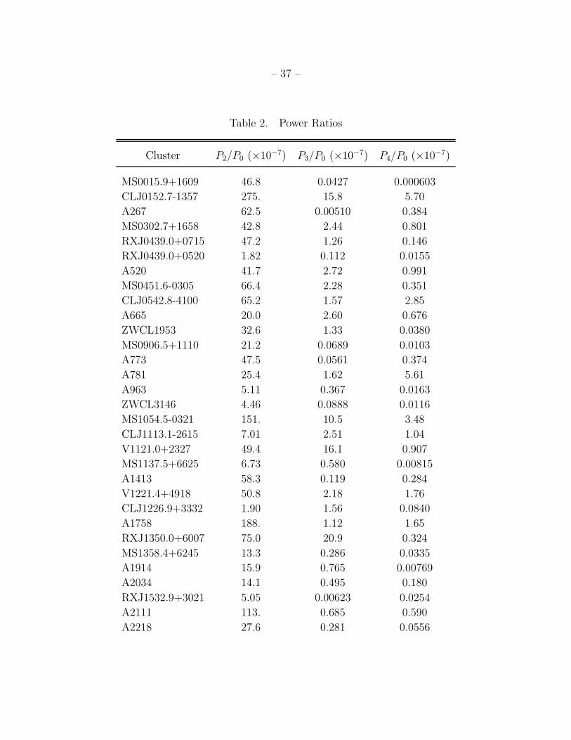
– 37 –

Table 2. Power Ratios

Cluster P2/P0 (×10−7) P3/P0 (×10−7) P4/P0 (×10−7)

MS0015.9+1609 46.8 0.0427 0.000603

CLJ0152.7-1357 275. 15.8 5.70

A267 62.5 0.00510 0.384

MS0302.7+1658 42.8 2.44 0.801

RXJ0439.0+0715 47.2 1.26 0.146

RXJ0439.0+0520 1.82 0.112 0.0155

A520 41.7 2.72 0.991

MS0451.6-0305 66.4 2.28 0.351

CLJ0542.8-4100 65.2 1.57 2.85

A665 20.0 2.60 0.676

ZWCL1953 32.6 1.33 0.0380

MS0906.5+1110 21.2 0.0689 0.0103

A773 47.5 0.0561 0.374

A781 25.4 1.62 5.61

A963 5.11 0.367 0.0163

ZWCL3146 4.46 0.0888 0.0116

MS1054.5-0321 151. 10.5 3.48

CLJ1113.1-2615 7.01 2.51 1.04

V1121.0+2327 49.4 16.1 0.907

MS1137.5+6625 6.73 0.580 0.00815

A1413 58.3 0.119 0.284

V1221.4+4918 50.8 2.18 1.76

CLJ1226.9+3332 1.90 1.56 0.0840

A1758 188. 1.12 1.65

RXJ1350.0+6007 75.0 20.9 0.324

MS1358.4+6245 13.3 0.286 0.0335

A1914 15.9 0.765 0.00769

A2034 14.1 0.495 0.180

RXJ1532.9+3021 5.05 0.00623 0.0254

A2111 113. 0.685 0.590

A2218 27.6 0.281 0.0556

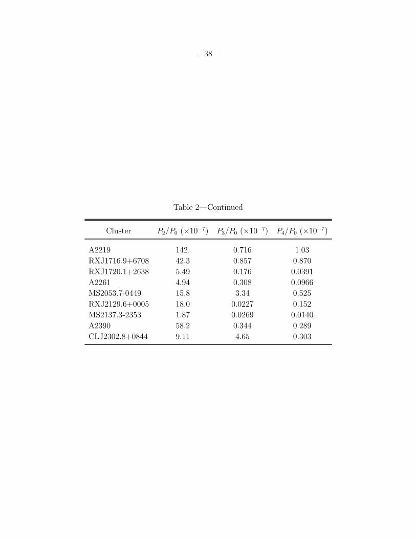
– 38 –

Table 2—Continued

Cluster P2/P0 (×10−7) P3/P0 (×10−7) P4/P0 (×10−7)

A2219 142. 0.716 1.03

RXJ1716.9+6708 42.3 0.857 0.870

RXJ1720.1+2638 5.49 0.176 0.0391

A2261 4.94 0.308 0.0966

MS2053.7-0449 15.8 3.34 0.525

RXJ2129.6+0005 18.0 0.0227 0.152

MS2137.3-2353 1.87 0.0269 0.0140

A2390 58.2 0.344 0.289

CLJ2302.8+0844 9.11 4.65 0.303

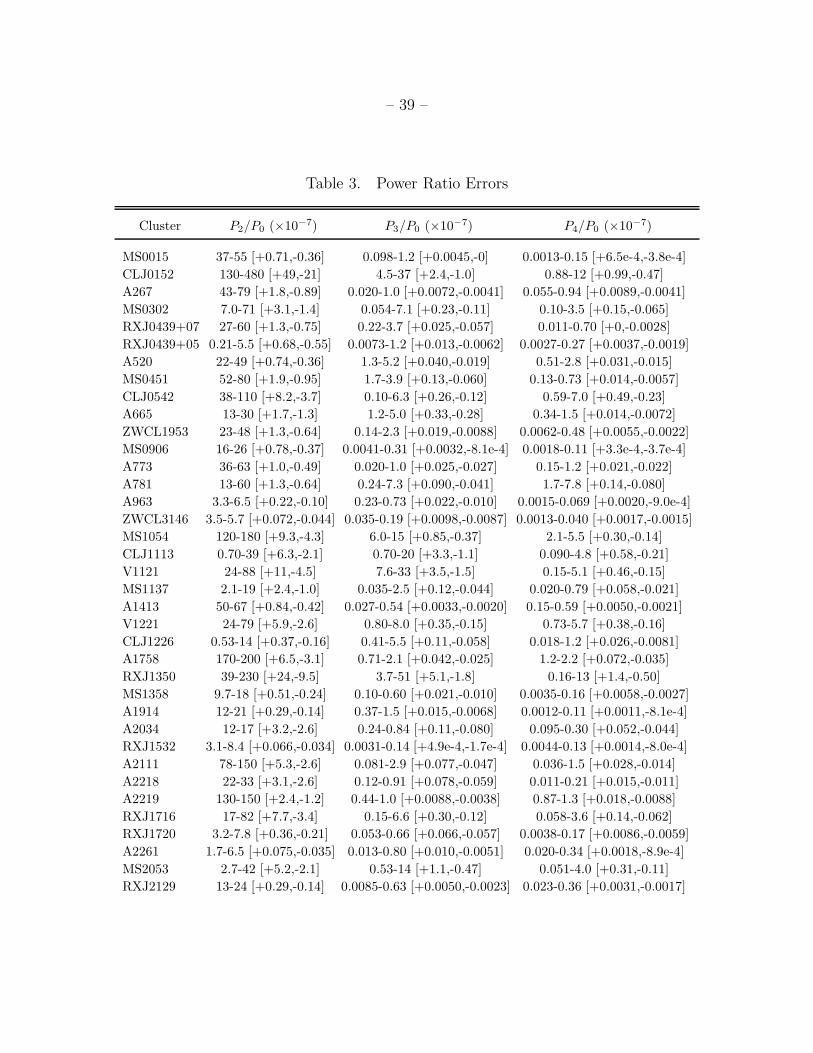
– 39 –

Table 3. Power Ratio Errors

Cluster P2/P0 (×10−7) P3/P0 (×10−7) P4/P0 (×10−7)

MS0015 37-55 [+0.71,-0.36] 0.098-1.2 [+0.0045,-0] 0.0013-0.15 [+6.5e-4,-3.8e-4]

CLJ0152 130-480 [+49,-21] 4.5-37 [+2.4,-1.0] 0.88-12 [+0.99,-0.47]

A267 43-79 [+1.8,-0.89] 0.020-1.0 [+0.0072,-0.0041] 0.055-0.94 [+0.0089,-0.0041]

MS0302 7.0-71 [+3.1,-1.4] 0.054-7.1 [+0.23,-0.11] 0.10-3.5 [+0.15,-0.065]

RXJ0439+07 27-60 [+1.3,-0.75] 0.22-3.7 [+0.025,-0.057] 0.011-0.70 [+0,-0.0028]

RXJ0439+05 0.21-5.5 [+0.68,-0.55] 0.0073-1.2 [+0.013,-0.0062] 0.0027-0.27 [+0.0037,-0.0019]

A520 22-49 [+0.74,-0.36] 1.3-5.2 [+0.040,-0.019] 0.51-2.8 [+0.031,-0.015]

MS0451 52-80 [+1.9,-0.95] 1.7-3.9 [+0.13,-0.060] 0.13-0.73 [+0.014,-0.0057]

CLJ0542 38-110 [+8.2,-3.7] 0.10-6.3 [+0.26,-0.12] 0.59-7.0 [+0.49,-0.23]

A665 13-30 [+1.7,-1.3] 1.2-5.0 [+0.33,-0.28] 0.34-1.5 [+0.014,-0.0072]

ZWCL1953 23-48 [+1.3,-0.64] 0.14-2.3 [+0.019,-0.0088] 0.0062-0.48 [+0.0055,-0.0022]

MS0906 16-26 [+0.78,-0.37] 0.0041-0.31 [+0.0032,-8.1e-4] 0.0018-0.11 [+3.3e-4,-3.7e-4]

A773 36-63 [+1.0,-0.49] 0.020-1.0 [+0.025,-0.027] 0.15-1.2 [+0.021,-0.022]

A781 13-60 [+1.3,-0.64] 0.24-7.3 [+0.090,-0.041] 1.7-7.8 [+0.14,-0.080]

A963 3.3-6.5 [+0.22,-0.10] 0.23-0.73 [+0.022,-0.010] 0.0015-0.069 [+0.0020,-9.0e-4]

ZWCL3146 3.5-5.7 [+0.072,-0.044] 0.035-0.19 [+0.0098,-0.0087] 0.0013-0.040 [+0.0017,-0.0015]

MS1054 120-180 [+9.3,-4.3] 6.0-15 [+0.85,-0.37] 2.1-5.5 [+0.30,-0.14]

CLJ1113 0.70-39 [+6.3,-2.1] 0.70-20 [+3.3,-1.1] 0.090-4.8 [+0.58,-0.21]

V1121 24-88 [+11,-4.5] 7.6-33 [+3.5,-1.5] 0.15-5.1 [+0.46,-0.15]

MS1137 2.1-19 [+2.4,-1.0] 0.035-2.5 [+0.12,-0.044] 0.020-0.79 [+0.058,-0.021]

A1413 50-67 [+0.84,-0.42] 0.027-0.54 [+0.0033,-0.0020] 0.15-0.59 [+0.0050,-0.0021]

V1221 24-79 [+5.9,-2.6] 0.80-8.0 [+0.35,-0.15] 0.73-5.7 [+0.38,-0.16]

CLJ1226 0.53-14 [+0.37,-0.16] 0.41-5.5 [+0.11,-0.058] 0.018-1.2 [+0.026,-0.0081]

A1758 170-200 [+6.5,-3.1] 0.71-2.1 [+0.042,-0.025] 1.2-2.2 [+0.072,-0.035]

RXJ1350 39-230 [+24,-9.5] 3.7-51 [+5.1,-1.8] 0.16-13 [+1.4,-0.50]

MS1358 9.7-18 [+0.51,-0.24] 0.10-0.60 [+0.021,-0.010] 0.0035-0.16 [+0.0058,-0.0027]

A1914 12-21 [+0.29,-0.14] 0.37-1.5 [+0.015,-0.0068] 0.0012-0.11 [+0.0011,-8.1e-4]

A2034 12-17 [+3.2,-2.6] 0.24-0.84 [+0.11,-0.080] 0.095-0.30 [+0.052,-0.044]

RXJ1532 3.1-8.4 [+0.066,-0.034] 0.0031-0.14 [+4.9e-4,-1.7e-4] 0.0044-0.13 [+0.0014,-8.0e-4]

A2111 78-150 [+5.3,-2.6] 0.081-2.9 [+0.077,-0.047] 0.036-1.5 [+0.028,-0.014]

A2218 22-33 [+3.1,-2.6] 0.12-0.91 [+0.078,-0.059] 0.011-0.21 [+0.015,-0.011]

A2219 130-150 [+2.4,-1.2] 0.44-1.0 [+0.0088,-0.0038] 0.87-1.3 [+0.018,-0.0088]

RXJ1716 17-82 [+7.7,-3.4] 0.15-6.6 [+0.30,-0.12] 0.058-3.6 [+0.14,-0.062]

RXJ1720 3.2-7.8 [+0.36,-0.21] 0.053-0.66 [+0.066,-0.057] 0.0038-0.17 [+0.0086,-0.0059]

A2261 1.7-6.5 [+0.075,-0.035] 0.013-0.80 [+0.010,-0.0051] 0.020-0.34 [+0.0018,-8.9e-4]

MS2053 2.7-42 [+5.2,-2.1] 0.53-14 [+1.1,-0.47] 0.051-4.0 [+0.31,-0.11]

RXJ2129 13-24 [+0.29,-0.14] 0.0085-0.63 [+0.0050,-0.0023] 0.023-0.36 [+0.0031,-0.0017]

– 40 –

Table 3—Continued

Cluster P2/P0 (×10−7) P3/P0 (×10−7) P4/P0 (×10−7)

MS2137 1.2-2.8 [+0.024,-0.0095] 0.0038-0.12 [+0.0014,-6.7e-4] 0.0035-0.066 [+2.1e-4,-8.7e-5]

A2390 52-67 [+0.074,-0.038] 0.17-1.0 [+0.0079,-0.044] 0.13-0.59 [+0.0036,-0.0021]

CLJ2302 0.74-42 [+6.5,-2.3] 0.81-19 [+3.7,-1.2] 0.067-3.7 [+0.58,-0.20]

Note. — 90% confidence intervals for the power ratios based on Monte Carlo simula-

tions. The average systematic errors from the normalization of the background are listed

in brackets.

Table 4. Statistical Significance of Results

Average Average Rank-Sum KS Prob. Average Average

Low-z High-z Prob. RS Prob. KS Prob.

P2/P0 3.92e-6 6.16e-6 0.10 0.34 - -

P3/P0 6.93e-8 5.95e-7 4.6e-5 0.00064 0.00036 0.0023

P4/P0 5.20e-8 1.30e-7 0.025 0.041 0.0082 0.037

Note. — Columns 1 and 2 give the average power ratios for the high and

low-redshift samples, respectively. Column 3 lists the probability from a rank-

sum test that the low and high-redshift clusters have the same average power

ratios. The probability from a KS-test that the two samples have the same

distribution is given in column 4. The last two columns list the average rank-

sum and KS probabilities for 1000 runs where the power ratios were randomly

selected from the Monte Carlo simulations.

– 41 –

Table 5. Noise Corrected Power Ratios

Cluster P2/P0 (×10−7) P3/P0 (×10−7) P4/P0 (×10−7)

MS0015.9+1609 46.4 0.316 -0.0459

CLJ0152.7-1357 264. 12.4 4.20

A267 61.4 -0.306 0.254

MS0302.7+1658 36.9 0.658 0.0479

RXJ0439.0+0715 46.2 0.961 0.0191

RXJ0439.0+0520 1.29 -0.0455 -0.0509

A520 40.7 2.43 0.870

MS0451.6-0305 66.1 2.19 0.316

CLJ0542.8-4100 61.3 0.332 2.31

A665 19.4 2.43 0.603

ZWCL1953 31.7 1.05 -0.0848

MS0906.5+1110 21.0 0.00166 -0.0181

A773 46.9 -0.125 0.297

A781 21.7 0.512 5.14

A963 5.03 0.342 0.00607

ZWCL3146 4.42 0.0780 0.00715

MS1054.5-0321 150. 10.3 3.37

CLJ1113.1-2615 -2.16 -0.482 -0.302

V1121.0+2327 45.0 14.7 0.322

MS1137.5+6625 5.24 0.115 -0.195

A1413 58.0 0.0525 0.256

V1221.4+4918 47.9 1.29 1.37

CLJ1226.9+3332 -0.821 0.770 -0.243

A1758 188. 1.06 1.62

RXJ1350.0+6007 58.8 15.7 -1.98

MS1358.4+6245 13.2 0.228 0.00851

A1914 15.7 0.709 -0.0157

A2034 14.1 0.476 0.172

RXJ1532.9+3021 4.89 -0.0389 0.00664

A2111 112. 0.210 0.386

A2218 27.4 0.233 0.0353

– 42 –

Table 5—Continued

Cluster P2/P0 (×10−7) P3/P0 (×10−7) P4/P0 (×10−7)

A2219 142. 0.700 1.02

RXJ1716.9+6708 37.8 -0.541 0.266

RXJ1720.1+2638 5.32 0.124 0.0175

A2261 4.57 0.201 0.0516

MS2053.7-0449 12.1 2.16 0.00641

RXJ2129.6+0005 17.6 -0.0814 0.108

MS2137.3-2353 1.81 0.00772 0.00588

A2390 58.0 0.291 0.267

CLJ2302.8+0844 1.41 2.21 -0.767

Table 6. Results After Noise Correction

Average Average Rank-Sum KS Prob. Slope

Low-z High-z Prob. vs. z

P2/P0 3.84e-6 5.67e-6 0.25 0.34 -

P3/P0 4.67e-8 4.39e-7 0.013 0.015 4.09e-7 (8.19e-8, 8.03e-7)

P4/P0 4.25e-8 6.17e-8 0.31 0.15 7.47e-8 (-2.57e-8, 2.22e-7)

Note. — Columns 1 and 2 give the average power ratios for the high and low-

redshift samples after the noise correction. Column 3 lists the probability from

a rank-sum test that the low and high-redshift clusters have the same average

power ratios. The probability from a KS-test that the two samples have the same

distribution is given in column 4. The last column lists the average slope of the

power ratios vs. z from 1000 fits using a least absolute deviation method and where

the power ratios were randomly selected from the Monte Carlo simulations. The

90% confidence limits on the slope are given in parentheses.