The evolution of popular music: USA 1960-2010:

Supporting Information

Matthias Mauch, Robert M. MacCallum, Mark Levy, Armand M. Leroi

15 October, 2014

Contents

M Materials and Methods 2M.1 The origin of the songs . . . . . . . . . . . . . . . . . . . . . . . . . . . . . . . . . . . 2M.2 Measuring Harmony. . . . . . . . . . . . . . . . . . . . . . . . . . . . . . . . . . . . . 2M.3 Measuring Timbre. . . . . . . . . . . . . . . . . . . . . . . . . . . . . . . . . . . . . . 3M.4 Making musical lexica . . . . . . . . . . . . . . . . . . . . . . . . . . . . . . . . . . . . 3M.5 Semantic lexicon annotation . . . . . . . . . . . . . . . . . . . . . . . . . . . . . . . . 4M.6 Topic extraction . . . . . . . . . . . . . . . . . . . . . . . . . . . . . . . . . . . . . . . 5M.7 Semantic topic annotations . . . . . . . . . . . . . . . . . . . . . . . . . . . . . . . . . 6M.8 User-generated tags . . . . . . . . . . . . . . . . . . . . . . . . . . . . . . . . . . . . . 7M.9 Identifying musical Styles clusters: k-means and silhouette scores . . . . . . . . . . . 7M.10 Diversity metrics . . . . . . . . . . . . . . . . . . . . . . . . . . . . . . . . . . . . . . 8M.11 Identifying musical revolutions . . . . . . . . . . . . . . . . . . . . . . . . . . . . . . . 9M.12 Identifying Styles that change around each revolution . . . . . . . . . . . . . . . . . . 10

S Supplementary Text & Tables 11

1

M Materials and Methods

M.1 The origin of the songs

Metadata on the complete Billboard Hot 100 charts were obtained through the (now defunct) BillboardAPI, consisting of artist name, track name, and chart position in every week of the charts from 1957 toearly 2010. We use only songs from 1960 through 2009 since these years have complete coverage. Usinga Last.fm’s proprietary matching procedure, we associated Last.fm MP3 audio recordings with the chartentries. Each recording is 30 seconds long. We use 17,094 songs, covering 86% of the weekly Billboardcharts (84% before 2000, 95% from 2000 onward (figure M1). This amounts to 69% of unique audiorecordings. The total duration of the music data is 143 hours.

1960 1970 1980 1990 2000 2010

020

4060

8010

0

by week

num

ber

of s

ongs

Figure M1: Coverage of the Billboard Hot 100 Charts by week.

To validate our impression that data quality was good, a random sub-sample of 9928 songs was vettedby hundreds of volunteers recruited on the internet. The participants were presented with two recordings,and for each were asked to to answer the question “Does recording [...] have very poor audio quality?”. Weanalysed those 5593 recordings that were judged at least twice. A recording was considered poor qualityif it was marked as such by a majority vote. Overall, this was the case in only 3.8% of the recordings,with a bias towards worse quality recordings in the 1960s (9.1%; 1970 and later: 1.8%). To examine theeffect of bad songs, we removed them and compared the estimated mean q of each topic (Section M.6) forthe total population versus the population of ‘good’ songs for each year of the 1960s. In no case did wefind that they were significantly different. We conclude that recording quality will have a negligible effecton our results.

All songs were decoded to PCM WAV format (44100 Hz, 16 bit). The songs were then band-pass-filtered using the Audio Degradation Toolbox [1] to reduce differences in recording equalisation in thebass and high treble frequencies (stop-band frequencies: 67 Hz, 6000 Hz).

M.2 Measuring Harmony.

The harmony features consist of 12-dimensional chroma features (also: pitch class profiles) [2]. Chromais widely used in MIR as a robust feature for chord and key detection [3], audio thumbnailing [4], andautomatic structural segmentation [5]. In every frame chroma represents the activations (i.e. the strength)

c = (c1, . . . , c12)

corresponding to the 12 pitch classes in the chromatic musical scale (i.e. that of the piano): A, B[, B C,. . . , G, A[. We use the NNLS Chroma implementation [6] to extract chroma at the same frame rate asthe timbre features (step size: 1024 samples = 23ms, i.e. 43 per second), but with the default frame size

2

of 16384 samples. The chroma representation (often called chromagram) of the complete 30 s excerpt of“Bohemian Rhapsody” is shown in figure 1 (main text).

M.3 Measuring Timbre.

The timbre features consist of 12 Mel-frequency cepstral coefficients (MFCCs), one delta-MFCC value, andone Zero-crossing Count (ZCC) feature. MFCCs are spectral-domain audio features for the descriptionof timbre and are routinely used in speech recognition [7] and Music Information Retrieval (MIR) tasks[8]. For every frame, they provide a low-dimensional parametrisation of the overall shape of the signal’sMel-spectrum, i.e. a spectral representation that takes into account human near-logarithmic perceptionof sound in magnitude (log-magnitude) and frequency (Mel scale). We use the first 12 MFCCs (excludingthe 0th component) and additionally one delta-MFCC, calculated as the difference between any twoconsecutive values of the 0th MFCC component. The MFCCs were extracted using a plugin from theVamp library (link retrieved 27.03.2014) with the default parameters (block size: 2048 samples = 46ms,step size: 1024 samples = 23ms). This amounts to ≈ 43 frames per second. The ZCC (also: zero-crossingrate, ZCR) is a time-domain audio feature which has been used in speech recognition [9] and has beenapplied successfully to discern drum sounds [10]. It is calculated by simply counting the number of timesconsecutive samples in a frame are of opposite sign. ZCC is high for noisy signals and transient sounds atthe onset of consonants and percussive events. To extract the ZCC we also used a Vamp plugin, extractingfeatures at the same frame rate (43 per second, step size: 1024 sampes = 23ms), but with a block sizeof 1024 samples. MFCCs and zero crossing counts of “Bohemian Rhapsody” are shown in figure 1 (maintext).

M.4 Making musical lexica

Since we aim to apply topic models to our data (see Section M.6), we need to discretise our raw featuresinto musical lexica. We have one timbral lexicon (T-Lexicon) and one harmonic lexicon (H-Lexicon).

Timbre.

In order to define the T-Lexicon we followed an unsupervised feature learning approach by quantisingthe feature space into 35 discrete classes as follows. First, we randomly selected 20 frames from eachof 11350 randomly selected songs (227 from every year), a total of 227,000 frames. The features werethen standardised, and de-correlated using principal component analysis (PCA). The PCA componentswere once more standardised. We then applied model-based clustering (Gaussian mixture models, GMM)to the standardised de-correlated data, using the built-in Matlab function gmdistribution.fit with fullcovariance matrix [11]. The GMM with 35 mixtures (clusters) was chosen as it minimised the BayesInformation Criterion. We then transformed all songs according to the same PCA, scaling and clustermapping transformations. In particular, every audio frame was assigned to its most likely cluster accordingto the GMM. Frames with cluster probabilities of < 0.5 were removed.

Harmony.

Our H-Lexicon consists of all 192 possible changes between the most frequently used chord types inpopular music [12]: major (M), minor (m), dominant 7 (7) and minor 7 chords (m7). We use chordchanges because they offer a key-independent way of describing the temporal dynamics of harmony. As achord is defined by its root pitch class (A,Bb,B,C,. . . ,Ab[) and its type, our system gives rise to 4×12 = 48chords. Each of the chords can be represented as a binary chord template with 12 elements correspondingto the twelve pitch classes. For example, the four chords with root A are these.

CTAM = (1, 0, 0, 0, 1, 0, 0, 1, 0, 0, 0, 0)

3

-�

m8→ M

Gm to E[M

Figure M2: Chord activation, with the most salient chords at any time highlighted in blue. Excerpt of“Bohemian Rhapsody” by Queen.

CTAm = (1, 0, 0, 1, 0, 0, 0, 1, 0, 0, 0, 0)

CTA7 = (1, 0, 0, 0, 1, 0, 0, 1, 0, 0, 1, 0)

CTAm7 = (1, 0, 0, 1, 0, 0, 0, 1, 0, 0, 1, 0)

At every frame we estimate the locally most likely chord by correlating the chroma vectors (Section M.2)with the binary chord templates (see, e.g. [13]), i.e. a given chroma frame c = (c1, . . . , c12) is correlatedto a chord template CT = (CT 1, . . . ,CT 12) by using Pearson’s rho,

ρCT ,c =

12∑i=1

(CT i − CT )(ci − c)

σCTσc,

where the bar over variables denotes the sample mean and σ· denotes the sample standard deviation ofthe corresponding vector. To smooth these correlation scores over time, we apply a median filter of length43 (1 second). An example of the resulting smoothed chord activation matrix is shown in figure M2. Wethen choose the chord with the highest median-smoothed correlation and combine the two chord labelsspaced 1 second apart into one chord change label, retaining only the relative root positions of the chordsand both chord types [14], as demonstrated in figure M2. If the chord change was ambiguous (meancorrelation of the two chords < 0.4), the chord change label was set to an additional 193rd label NA.

In summary, we have obtained two lexica of frame-wise discrete labels, one for timbre (35 classes) andone for harmony (193 chord changes). Each allows us to describe a piece of music as a count vector givingcounts of timbre classes and chord changes, respectively.

M.5 Semantic lexicon annotation

Since we can now express our music in terms of lexica of discrete items, we can attach human-readablelabels to these items. In the case of the 193 chord changes (H-Lexicon), an intrinsic musical interpretationexists. The most frequent chord changes are given in additional online tables (Section 3), along with someexplanations and counts over the whole corpus.

The 35 classes in the T-Lexicon do not have a priori interpretations, so we obtained human annotationson a subset of our data. First, we randomly selected 100 songs, two from each year, and concatenated

4

the audio that belonged to the same of the 35 sound classes from our T-Lexicon using an overlap-addapproach. That is, each audio file contained frames from only one of the timbre classes introduced inSection M.4, but from up to 100 songs. The resulting 35 sound class files can be accessed on SoundCloud1).We noticed that each of the files does indeed have a timbre characteristic; some captured a particularvowel sound, others noisy hi-hat and crash cymbal sounds, others again very short, percussive sounds.We then asked ten human annotators to individually describe these sounds. Each annotator listened toall 35 files and, for each, subjectively chose 5 terms that described the sound from a controlled vocabularyconsisting of the following 34 labels manually compiled from initial free-vocabulary annotations:

mellow, aggressive, dark, bright, calm, energetic, smooth, percussive, quiet, loud, harmonic, noisy,melodic, rounded, harsh, vocal, instrumental, speech, instrument: drums, instrument: guitar, instrument:piano, instrument: orchestra, instrument: male voice, instrument: female voice, instrument: synthesiser,‘ah’, ‘ay’, ‘ee’, ‘er’, ‘oh’, ‘ooh’, ‘sh’, ‘ss’, [random – I find it hard to judge].

On average, the most agreed-upon label per class was chosen by 7.5 (mean) of the 10 annotators,indicating good agreement. Even the second- and third-ranking labels were chosen by more than half ofthe annotators (means 6.4 and 5.68). Figure M3 shows the agreement of the top labels from rank 1 to 8.

●

●

●

●

●●

●●

1 2 3 4 5 6 7 8

0

2

4

6

8

rank of most agreed−upon sound labels

mea

n #

of a

nnot

ator

s (o

f 10)

Figure M3: Agreement of the 10 annotators in the semantic sound annotation task.

M.6 Topic extraction

For timbre and harmony separately, a topic model is estimated from the song-wise counts, using theimplementation of Latent Dirichlet Allocation (LDA) [15] provided in the topicmodels library [16] forR. LDA is a hierarchical generative model of a corpus. The original model was formulated in the contextof a text corpus in which

a) every document (here: song) is represented as a discrete distribution over NT topics

b) every every topic is represented as a discrete distribution over all possible words (here: H-Lexiconor T-Lexicon entries)

Since the T- and H-Lexicon count vectors introduced in Section M.4 are of the same format as wordcounts, we can apply the same modelling procedure. That is, by means of probabilistic inference on themodel, the LDA method estimates the topic distributions of each song (probabilities of a song using aparticular topic) and the topics’ lexical distribution (probabilities over the H- and T-lexica) from thelexicon count vectors.

We used the LDA function, which implements the variational expectation-maximization (VEM) algo-rithm to estimate the parameters, setting the number of topics to 8. Hence, we obtained one model with

1https://soundcloud.com/descent-of-pop/sets/cluster-sounds

5

8 T-Topics, and one with 8 H-Topics. Topic models allow us to encode every song as a distribution overT- and H-Topics,

qT = (qT1 , qT2 , . . . , q

T8 )

qH = (qH1 , qH2 , . . . , q

H8 )

The probabilities can be interpreted as the proportion of frames in the song belonging to the topic.When it is clear from the context which T- or H-Topic we are concerned with we denote these by theletter q, and their mean over a group of songs by q. Mean values by year for all topics are shown infigure 2 in the main text with 95% confidence intervals based on quantile bootstrapping.

In the same manner, we calculate means and bootstrap confidence intervals for all artists with at least10 chart entries and all Last.fm tags (introduced in Section M.8) with at least 200 occurrences. Theartists with the highest and lowest mean q of each topic and the respective listing of tags can be found inadditional online tables (Sections 1 and 2).

M.7 Semantic topic annotations

In this section we show how to map the semantic interpretations of our harmony and timbre lexica (seeSection M.5) to the 8 T-Topics and 8 H-Topics. This allows us to work with the topics rather than thelarge number of chord changes and sound classes.

Harmony.

Each H-Topic is defined as a distribution P (EHi ) over all H-lexicon entries EH

i , i = 1, . . . , 193 (the 193different chord changes). The most most probable chord changes for each topic can be found in ouradditional online tables (Section 3). For example, the most likely chord change in H-Topic 4 is a Majorchord followed by another Major chord 7 semitones higher, e.g. C to G. The interpretation of a topic,then, is the coincidence of such chord changes in a piece of music. Interpretations of the 8 H-Topics canbe found in Table 1.

Timbre.

In order to obtain interpretations for the T-Topics we map the semantic annotations of the T-lexicon(Section M.5) to the topics. The semantic annotations of the T-lexicon come as a matrix of countsW ∗ = (w∗

ij) of annotation labels j = 1, . . . , 34 for each of the sound classes i = 1, . . . , 35. We firstnormalise the columns w∗

·,j by root-mean-square normalisation to obtain a scaled matrix Wij with theelements

wij =w∗

ij√(1/34)

∑i(w

∗ij)

2. (1)

The matrix W = (wij) expresses the relevance of the jth label for the ith sound class. Since T-Topics arecompositions of sound classes, we can now simply map these relevance values to the topics by multipli-cation. The weight Lj of the jth label for a T-Topic in which sound class ET

i appears with probabilityP (ET

i ) is

Lj =

35∑i=1

wijP (ETi ). (2)

The top 3 labels for each T-Topic can be found in Table 1.

6

Table 1: Topic interpretations.

harmonic topics

H1 changes involving dominant 7th chordsH2 natural minor key changesH3 changes involving minor 7th chordsH4 simple diatonic changes used in major keysH5 unrecognised changes or no chordal contentH6 stepwise changes indicating modal harmonyH7 ambiguous major/minor attributionH8 sustained major chords

timbral topics

T1 drums, aggressive, percussiveT2 calm, quiet, mellowT3 energetic, speech, brightT4 piano, orchestra, harmonicT5 guitar, loud, energeticT6 ay, male voice, vocalT7 oh, rounded, mellowT8 female voice, melodic, vocal

M.8 User-generated tags

The Last.fm recordings are also associated with tags, generated by Last.fm users, which we obtained via aproprietary process. The tags are usually genre-related (POP, SOUL), but a few also contain informationabout the instrumentation (e.g. PIANO), feel (e.g. SUMMER), references to particular artists and others.We removed references to particular artists and joined some tags that were semantically identical. Afterthe procedure we had tags for 16085 (94%) of the songs, with a mean tag count of 2.7 per song (median:3, mode: 4).

M.9 Identifying musical Styles clusters: k-means and silhouette scores

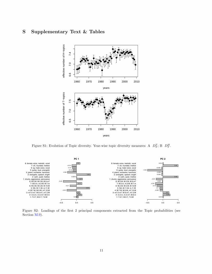
In order to identify musical styles from our data measurements, we first used the 17094 × 16 (i.e. songs× topics) data matrix of all topic probabilities qT and qH , and de-correlated the data using PCA (seealso figure S2). The resulting data matrix has 14 non-degenerate principal components, which we usedto cluster the data using k-means clustering. We chose a cluster number of 13 based on analysing ofthe mean silhouette width [17] over a range of k = 2, . . . , 25 clusters, each started with 50 randominitialisations. The result of the best clustering at k = 13 is chosen, and each song is thus classified to astyle s ∈ {1, . . . , 13} (figure M4).

7

5 10 15 20 25

0.11

00.

115

0.12

00.

125

0.13

00.

135

0.14

0

number of clusters

mea

n si

lhou

ette

sco

re

●

●

●●

●

●

●

●

●●

● ●

●●

●

●

●

●

●

●

●

●

●●

●

Figure M4: Mean silhouette scores. The optimal number of clusters, k = 13 is highlighted in blue.

M.10 Diversity metrics

In order assess the diversity of a set of songs (usually the songs having entered the charts in a certainyear) we calculate four different metrics: number of songs (DN ), effective number of styles (style diversity,DC), effective number of topics (topic diversity, DT ) and disparity (total standard deviation, DY ). Thefollowing paragraphs explain these metrics.

Number of songs.

The simplest measure of complexity is the number of songs DN . We use it to show that other diversitymetrics are not intrinsically linked to this measure.

Effective number of Styles.

In the ecology literature, diversity refers to the effective number of species in an ecosystem. Maximumdiversity is achieved when the species’ frequencies are all equal, i.e. when they are uniformly distributed.Likewise, minimum diversity is assumed when all organisms belong to the same species. According to[18], diversity for a population of Ns species can formally be defined as

DS = exp

(−

Ns∑i=1

si ln si

)(3)

where si, i = 1, . . . , Ns represents the relative frequency distribution over the Ns species such that∑

i si =1. In particular, the maximum value assumed when all species’ relative frequencies are equal is D = Ns.If, on the other hand, only one species remains, and all others have frequencies of zero, then D = 1, theminimum value.

We use this exact definition to describe the year-wise diversity of acoustical Style clusters in ourdata (recall that each song has only one Style, but a mixture of Topics). For every year we calculate

8

the proportion songs si, i = 1, . . . , 13 belonging to each of the 13 Styles, and hence we use Ns = 13 tocalculate DS ∈ [1, 13].

Effective number of Topics.

The probability q of a certain topic in a song (see Section M.6) provides an estimate of the proportionof frames in a song that belong to that topic. By averaging over the year, we can get an estimate of theproportion q of frames in the whole year, i.e. for all T- and H-Topics we obtain the yearly measurements

qT = (qT1 , qT2 , . . . , q

T8 )

qH = (qH1 , qH2 , . . . , q

H8 ).

Figuratively, we throw all audio frames of all songs into one big bucket pertaining to a year, and estimatethe proportion of each topic in the bucket. From these yearly estimates of topic frequencies we can nowcalculate the effective number of T- and H-Topics in the same way we calculated the effective number ofStyles (figure S1).

DTT = exp

(−

8∑i=1

qTi ln qTi

)(4)

DHT = exp

(−

8∑i=1

qHi ln qHi

)(5)

DT :=DT

T +DHT

2, (6)

where we define DT as the overall measure of topic diversity. DT is shown in the main manuscript (figure4). The individual H- and T-Topic diversities DT

T and DHT are provided in figure S1. It is evident that

the significant diversity decline in the 1980s is mainly due to a decline in timbral topic diversity, whileharmonic diversity shows no sign of sustained decline.

Disparity.

In contrast to diversity, disparity corresponds to morphological variety, variety of measurements. Twoecosystems of equal diversity can have different disparity, depending on the extent to which the phenotypesof species differ. A variety of measures, such as average pairwise character dissimilarity and the totalvariance (sum of univariate variance) [19, 20] have been used to measure disparity. We adopt the squareroot of total variance, a metric called total standard deviation [21, p. 37] as our measure of disparity, i.e.given a set of N observations on T traits as a matrix X = (xn,m), we define it as

DY =

√√√√ T∑t=1

Var(x·,m). (7)

We apply our disparity measure DY to the 14-dimensional matrix of principal components (derivedfrom the topics, as described in Section M.9).

M.11 Identifying musical revolutions

In order to identify points at which the composition of the charts significantly changes, we employ Footenovelty detection [22], a technique often used in MIR [23]. First we pool the 14-dimensional principalcomponent data (see Section M.9) into quarters by their first entry into the charts (January-March, April-June, July-September, October-December) using the quarterly mean of each principal component. We

9

then construct a matrix (see figure 5 in main text) of pairwise distances between each quarter. Foote’smethod consists of convolving such a distance matrix with a so-called checkerboard kernel along the maindiagonal of the matrix. Checkerboard kernels represent the stylised case of homogeneity within regions(low values in the upper right and bottom-left quadrants) and dissimilarity between regions (high valuesin the other two quadrants). In such a situation, i.e. when one homogenous era transitions to another,the convolution results in high values.

A kernel with a half-width of 12 quarters (3 years) compares the 3 years prior to the current quarter tothose following the current quarter (figure M5). We follow Foote [22] in using checkerboard kernels withGaussian taper (standard deviation: 0.4 times the half-width). The kernel matrix entries correspondingto the central, “current” quarter are set to zero.

Many different kernel widths are possible. Figure 5B in the main text shows the novelty score forkernels with half-widths between 4 quarters (1 year) and 50 quarters (12.5 years). We can clearly makeout three major ‘revolutions’ (early 1960s, early 1980s, early 1990s) that result in high novelty scores fora wide range of kernel sizes.

−10 −5 0 5 10

−10

−50

510

lag/months

lag/months

Figure M5: Foote checkerboard kernel for novelty detection.

In order to be able to assess the significance of these regions we compared their novelty scores againstnovelty values obtained from randomly permuted distance matrices. We first repeated the process 1000times on distance matrices with randomly permuted quarters. For every kernel size we then calculatedthe quantiles at confidence levels α = 0.95, 0.99 and 0.999. The results are shown as contour lines infigure 5B in the main text.

For further analysis we choose the time scale depicted with a half-width lag of 12 quarters (3 years).This results in three change regions at confidence p < 0.01. The ‘revolution’ points are the points ofmaximum Foote novelty within the three regions of significant change.

M.12 Identifying Styles that change around each revolution

To identify the styles (clusters) that change around each revolution, we obtained the frequencies of eachstyle for the 24 quarters flanking the peak of a revolution, and estimated the rate of change per annumby a quadratic model. We then used a tag-enrichment analysis to identify those tags associated with eachstyle just around each revolution, see Table S2.

10

S Supplementary Text & Tables

●●●

●●

●●●

●●

●

●

●●

●

●●

●●

●●

●

●●●

●

●

●

●●

●

●●

●

●

●

●

●●●

●●

●●

●●

●

●●

●

1960 1970 1980 1990 2000 2010

6.6

7.0

7.4

years

effe

ctiv

e nu

mbe

r of

H−

topi

cs

●●●

●●

●●●

●●

●

●

●●

●

●●

●●

●●

●

●●●

●

●

●

●●

●

●●

●

●

●

●

●●●

●●

●●

●●

●

●●

●

●

●●●

●●

●●

●●●

●●

●

●●

●●

●

●●

●

●

●

●

●

●●

●●

●●

●

●●

●●

●

●

●

●●●●

●

●

●

●●

●

1960 1970 1980 1990 2000 2010

6.5

7.0

7.5

years

effe

ctiv

e nu

mbe

r of

T−

topi

cs

●

●●●

●●

●●

●●●

●●

●

●●

●●

●

●●

●

●

●

●

●

●●

●●

●●

●

●●

●●

●

●

●

●●●●

●

●

●

●●

●

Figure S1: Evolution of Topic diversity. Year-wise topic diversity measures: A DTT ; B DH

T .

1: 7.0.7, M.0.7, 7.0.M2: m.0.m, m.0.m7, M.9.m

3: m7.0.m7, M.9.m7, m7.3.M4: M.7.M, M.5.M, m7.10.M

5: NA, M.11.M, m.11.M6: M.2.M, M.5.M, M.10.M

7: M.0.m, m.0.M, M.7.m8: M.0.M, M.5.M, M.9.m7

1: drums, aggressive, percussive2: calm, quiet, mellow

3: energetic, speech, bright4: piano, orchestra, harmonic

5: guitar, loud, energetic6: ay, male voice, vocal7: oh, rounded, mellow

8: female voice, melodic, vocal

PC 1

−0.5 0.0 0.5

0.0580.17

0.12−0.32

0.43−0.21

0.17−0.43

0.20.0078

0.46−0.29

−0.12−0.14−0.16

0.12

1: 7.0.7, M.0.7, 7.0.M2: m.0.m, m.0.m7, M.9.m

3: m7.0.m7, M.9.m7, m7.3.M4: M.7.M, M.5.M, m7.10.M

5: NA, M.11.M, m.11.M6: M.2.M, M.5.M, M.10.M

7: M.0.m, m.0.M, M.7.m8: M.0.M, M.5.M, M.9.m7

1: drums, aggressive, percussive2: calm, quiet, mellow

3: energetic, speech, bright4: piano, orchestra, harmonic

5: guitar, loud, energetic6: ay, male voice, vocal7: oh, rounded, mellow

8: female voice, melodic, vocal

PC 2

−0.5 0.0 0.5

0.0130.240.2

−0.091−0.1

−0.19−0.24

−0.021−0.22

0.49−0.039−0.038

−0.49−0.043

0.490.014

1: X7.0.7, M.0.7, X7.0.M2: m.0.m, m.0.m7, M.9.m

3: m7.0.m7, M.9.m7, m7.3.M4: M.7.M, M.5.M, m7.10.M

5: NA, M.11.M, m.11.M6: M.2.M, M.5.M, M.10.M

7: M.0.m, m.0.M, M.7.m8: M.0.M, M.5.M, M.9.m7

1: drums, aggressive, percussive2: calm, quiet, mellow

3: energetic, speech, bright4: piano, orchestra, harmonic

5: guitar, loud, energetic6: ay, male voice, vocal7: oh, rounded, mellow

8: female voice, melodic, vocal

PC 3

−0.5 0.0 0.5

−0.09−0.36

−0.450.27

0.40.073

−0.120.3

−0.190.13

0.36−0.3

−0.160.120.11

0.031

1: X7.0.7, M.0.7, X7.0.M2: m.0.m, m.0.m7, M.9.m

3: m7.0.m7, M.9.m7, m7.3.M4: M.7.M, M.5.M, m7.10.M

5: NA, M.11.M, m.11.M6: M.2.M, M.5.M, M.10.M

7: M.0.m, m.0.M, M.7.m8: M.0.M, M.5.M, M.9.m7

1: drums, aggressive, percussive2: calm, quiet, mellow

3: energetic, speech, bright4: piano, orchestra, harmonic

5: guitar, loud, energetic6: ay, male voice, vocal7: oh, rounded, mellow

8: female voice, melodic, vocal

PC 4

−0.5 0.0 0.5

0.610.056

−0.42−0.32

−0.01−0.18

0.320.037

−0.22−0.12−0.045

0.19−0.1

0.290.11

−0.016

1: X7.0.7, M.0.7, X7.0.M2: m.0.m, m.0.m7, M.9.m

3: m7.0.m7, M.9.m7, m7.3.M4: M.7.M, M.5.M, m7.10.M

5: NA, M.11.M, m.11.M6: M.2.M, M.5.M, M.10.M

7: M.0.m, m.0.M, M.7.m8: M.0.M, M.5.M, M.9.m7

1: drums, aggressive, percussive2: calm, quiet, mellow

3: energetic, speech, bright4: piano, orchestra, harmonic

5: guitar, loud, energetic6: ay, male voice, vocal7: oh, rounded, mellow

8: female voice, melodic, vocal

PC 5

−0.5 0.0 0.5

−0.20.34

−0.016−0.0081

−0.092−0.039

−0.140.035

−0.5−0.22

0.096−0.026

0.120.13

−0.140.67

1: X7.0.7, M.0.7, X7.0.M2: m.0.m, m.0.m7, M.9.m

3: m7.0.m7, M.9.m7, m7.3.M4: M.7.M, M.5.M, m7.10.M

5: NA, M.11.M, m.11.M6: M.2.M, M.5.M, M.10.M

7: M.0.m, m.0.M, M.7.m8: M.0.M, M.5.M, M.9.m7

1: drums, aggressive, percussive2: calm, quiet, mellow

3: energetic, speech, bright4: piano, orchestra, harmonic

5: guitar, loud, energetic6: ay, male voice, vocal7: oh, rounded, mellow

8: female voice, melodic, vocal

PC 6

−0.5 0.0 0.5

0.190.0033

−0.23−0.06

−0.20.063

0.250.11

−0.0270.34

−0.16−0.39

0.32−0.57

0.0480.23

1: X7.0.7, M.0.7, X7.0.M2: m.0.m, m.0.m7, M.9.m

3: m7.0.m7, M.9.m7, m7.3.M4: M.7.M, M.5.M, m7.10.M

5: NA, M.11.M, m.11.M6: M.2.M, M.5.M, M.10.M

7: M.0.m, m.0.M, M.7.m8: M.0.M, M.5.M, M.9.m7

1: drums, aggressive, percussive2: calm, quiet, mellow

3: energetic, speech, bright4: piano, orchestra, harmonic

5: guitar, loud, energetic6: ay, male voice, vocal7: oh, rounded, mellow

8: female voice, melodic, vocal

PC 7

−0.5 0.0 0.5

−0.510.54

−0.38−0.15

−0.00870.23

0.30.056

0.0430.0240.029

−0.016−0.0032

0.0630.12

−0.32

1: X7.0.7, M.0.7, X7.0.M2: m.0.m, m.0.m7, M.9.m

3: m7.0.m7, M.9.m7, m7.3.M4: M.7.M, M.5.M, m7.10.M

5: NA, M.11.M, m.11.M6: M.2.M, M.5.M, M.10.M

7: M.0.m, m.0.M, M.7.m8: M.0.M, M.5.M, M.9.m7

1: drums, aggressive, percussive2: calm, quiet, mellow

3: energetic, speech, bright4: piano, orchestra, harmonic

5: guitar, loud, energetic6: ay, male voice, vocal7: oh, rounded, mellow

8: female voice, melodic, vocal

PC 8

−0.5 0.0 0.5

0.0530.11

−0.24−0.056

0.230.049

−0.310.079

0.049−0.19

0.110.55

−0.088−0.62

0.0740.054

Figure S2: Loadings of the first 2 principal components extracted from the Topic probabilities (seeSection M.9).

11

Table S1: Enrichment analysis: Last.fm user tag over-representation for all Styles over the complete dataset (only those with P < 0.05)

Style 1 Style 2 Style 3 Style 4 Style 5 Style 6 Style 7

northernsoul hiphop easylistening funk rock femalevocal countrysoul rap country blues classicrock pop classiccountryhiphop gangstarap lovesong jazz pop rnb comb folkdance oldschool piano soul newwave motown rockabillyrap dirtysouth ballad instrumental garage soul southernrockvocaltrance dance classiccountry rocknroll comb hardrock gleehouse dancehall jazz northernsoul garagerock soundtrack

westcoast doowop rockabilly british musicalparty swingcomedy loungereggae malevocalnewjackswing 50sclassic singersongwritersexy romanticurban softrock

christmasacoustic

Style 8 Style 9 Style 10 Style 11 Style 12 Style 13

dance classicrock lovesong funk soul rocknewwave country slowjams blues rnb comb hardrockpop rock soul dance funk alternativeelectronic singersongwriter folk bluesrock disco classicrocksynthpop folkrock rnb comb newwave slowjams alt indi rock combfreestyle folk neosoul electronic dance hairmetalrock pop femalevocal synthpop neosoul poppunkeurodance softrock singersongwriter hiphop newjackswing punkrocknewjackswing acoustic hardrock smooth punktriphop romantic oldschoolsoul poprockfunk mellow metal

easylistening powerpopjazz emobeautiful numetalsmooth heavymetalsoftrock glamrockballad grunge

british

12

Table S2: Identifying Styles that change around each revolution and the associated over-represented genretags in the 24 quarters flanking the revolutions.

revo- style estim. estim.lution cluster (linear) p (quad.) p tags

1964 1 0.044 0.019 0.050 0.009 northernsoul, motown, soul, easylistening, jazz2 -0.014 0.291 0.008 0.528 comedy, funny, jazz, easylistening3 -0.177 0.000 0.014 0.631 easylistening, jazz, swing, lounge, doowop4 -0.060 0.118 -0.009 0.806 jazz, northernsoul, soul, instrumental, blues5 0.060 0.014 -0.041 0.081 garagerock, garage, british, psychedelic6 -0.171 0.000 -0.045 0.282 femalevocal, motown, northernsoul, soul, doowop7 -0.018 0.495 -0.003 0.908 british, folk, surf, malevocal, rocknroll comb8 0.062 0.000 0.010 0.441 garagerock, instrumental, northernsoul, surf, soul9 0.083 0.014 0.006 0.861 rocknroll comb, northernsoul, motown, soul, garage

10 -0.020 0.349 0.034 0.109 folk, easylistening, jazz, swing11 0.037 0.131 -0.022 0.349 garagerock, blues, soul, northernsoul, instrumental12 0.043 0.001 0.000 0.996 northernsoul, soul, motown13 0.121 0.000 -0.005 0.821 psychedelic, garagerock, psychedelicrock, motown, british

1983 1 0.031 0.350 -0.050 0.136 newwave, synthpop, disco2 0.024 0.189 0.010 0.569 oldschool, funk, comedy3 -0.112 0.000 0.021 0.426 lovesong, softrock, easylistening, romantic4 -0.022 0.448 -0.005 0.846 newwave, disco, progressiverock5 0.020 0.614 -0.019 0.617 newwave, rock, classicrock, progressiverock, pop, synthpop6 -0.013 0.598 -0.005 0.828 femalevocal, disco, pop, reggae, musical, soundtrack7 -0.098 0.003 0.015 0.598 newwave, classiccountry, softrock, newromantic, rock, southernrock8 0.173 0.000 -0.029 0.190 newwave, pop, rock, disco, synthpop9 -0.065 0.057 0.065 0.055 classicrock, rock, softrock, progressiverock, newwave, pop

10 -0.047 0.110 -0.004 0.882 lovesong, softrock11 0.048 0.089 -0.058 0.043 newwave, synthpop, rock, classicrock, hardrock12 -0.095 0.001 0.011 0.664 funk, disco, soul, smoothjazz, dance13 0.150 0.000 0.034 0.236 rock, classicrock, hardrock, newwave, progressiverock, southernrock,

powerpop, heavymetal, hairmetal

1991 1 0.034 0.161 -0.018 0.457 house, freestyle, synthpop, newwave, electronic, dance2 0.325 0.000 0.043 0.187 hiphop, rap, oldschool, newjackswing, gangstarap, eurodance, westcoast, dance3 0.056 0.011 0.011 0.596 ballad, lovesong4 0.005 0.822 -0.034 0.153 dance, hairmetal, hardrock, metal, newjackswing5 -0.085 0.003 0.003 0.901 rock, hardrock, hairmetal, pop, freestyle6 0.000 0.999 0.015 0.344 femalevocal, pop, slowjams, dance, rnb comb, ballad7 0.023 0.307 0.007 0.742 rock, hardrock, hairmetal8 -0.023 0.584 -0.023 0.576 dance, newjackswing, freestyle, pop, electronic, synthpop, newwave, australian9 -0.015 0.690 0.046 0.224 rock, pop, softrock, ballad, hardrock

10 0.042 0.235 0.008 0.813 slowjams, lovesong, rnb comb11 -0.065 0.016 0.030 0.248 newwave, dance, synthpop, hairmetal, rock, freestyle12 -0.035 0.447 -0.017 0.712 newjackswing, rnb comb, dance, slowjams, house, pop, soul13 -0.207 0.000 -0.112 0.023 hardrock, hairmetal, rock, classicrock, metal, heavymetal, thrashmetal,

madchester

13

References

[1] Mauch M, Ewert S. The Audio Degradation Toolbox and its Application to Robustness Evaluation.In: Proceedings of the 14th International Society of Music Information Retrieval Conference (ISMIR2013); 2013. p. 83–88.

[2] Fujishima T. Real Time Chord Recognition of Musical Sound: a System using Common Lisp Music.In: Proceedings of the International Computer Music Conference (ICMC 1999); 1999. p. 464–467.

[3] Mauch M, Dixon S. Simultaneous Estimation of Chords and Musical Context from Audio. IEEETransactions on Audio, Speech, and Language Processing. 2010;18(6):1280–1289.

[4] Bartsch MA, Wakefield GH. Audio thumbnailing of popular music using chroma-based representa-tions. IEEE Transactions on Multimedia. 2005;7(1):96–104.

[5] Muller M, Kurth F. Towards structural analysis of audio recordings in the presence of musicalvariations. EURASIP Journal on Applied Signal Processing. 2007;2007(1):163–163.

[6] Mauch M, Dixon S. Approximate note transcription for the improved identification of difficult chords.Proceedings of the 11th International Society for Music Information Retrieval Conference (ISMIR2010). 2010;p. 135–140.

[7] Davis S, Mermelstein P. Comparison of parametric representations for monosyllabic word recognitionin continuously spoken sentences. IEEE Transactions on Acoustics, Speech and Signal Processing.1980;28(4):357–366.

[8] Foote JT. Content-Based Retrieval of Music and Audio. Proceedings of SPIE. 1997;138:138–147.

[9] Ito M, Donaldson RW. Zero-crossing measurements for analysis and recognition of speech sounds.IEEE Transactions on Audio and Electroacoustics. 1971;19(3):235–242.

[10] Gouyon F, Pachet F, Delerue O. On the use of zero-crossing rate for an application of classification ofpercussive sounds. In: Proceedings of the COST G-6 Conference on Digital Audio Effects (DAFX-00);2000. p. 1–6.

[11] McLachlan GJ, Peel D. Finite Mixture Models. Hoboken, NJ: John Wiley & Sons; 2000.

[12] Burgoyne JA, Wild J, Fujinaga I. An expert ground-truth set for audio chord recognition andmusic analysis. In: Proceedings of the 12th International Conference on Music Information Retrieval(ISMIR 2011); 2011. p. 633–638.

[13] Papadopoulos H, Peeters G. Large-scale Study of Chord Estimation Algorithms Based on ChromaRepresentation and HMM. In: International Workshop on Content-Based Multimedia Indexing;2007. p. 53–60.

[14] Mauch M, Dixon S, Harte C, Fields B, Casey M. Discovering chord idioms through Beatles and RealBook songs. In: Proceedings of the 8th International Conference on Music Information Retrieval(ISMIR 2007); 2007. p. 255–258.

[15] Blei DM, Ng AY, Jordan MI. Latent dirichlet allocation. Journal of Machine Learning Research.2003;3:993–1022.

[16] Hornik K, Grun B. topicmodels: An R package for fitting topic models. Journal of StatisticalSoftware. 2011;40(13):1–30.

[17] Rousseeuw PJ. Silhouettes: a graphical aid to the interpretation and validation of cluster analysis.Journal of computational and applied mathematics. 1987;20:53–65.

14

[18] Jost L. Entropy and diversity. Oikos. 2006;113(2):363–375.

[19] Erwin DH. DISPARITY: MORPHOLOGICAL PATTERN AND DEVELOPMENTAL CONTEXT.Palaeontology. 2007;50(1):57–73.

[20] Foote M. The evolution of morphological diversity. Annual Review of Ecology and Systematics.1997;.

[21] Hallgrımsson B, Hall BK. Variation: A Central Concept in Biology. Academic Press; 2011.

[22] Foote J. Automatic audio segmentation using a measure of audio novelty. In: IEEE InternationalConference on Multimedia and Expo. vol. 1; 2000. p. 452–455.

[23] Smith JBL, Chew E. A Meta-Analysis of the MIREX Structure Segmentation Task. In: Proceedingsof the 14th International Society for Music Information Retrieval Conference; 2013. .

15