The Evolution of Popular Music: USA 1960–2010

Matthias Mauch,1∗ Robert M. MacCallum,2 Mark Levy,3 Armand M. Leroi2

1School of Electronic Engineering and Computer Science, Queen Mary University of London, E1 4NS.

United Kingdom, 2Division of Life Sciences, Imperial College London, SW7 2AZ. United Kingdom,3Last.fm, 5–11 Lavingdon Street, London, SE1 0NZ. United Kingdom

In modern societies, cultural change seems ceaseless. The flux of fashion is especiallyobvious for popular music. While much has been written about the origin and evolutionof pop, most claims about its history are anecdotal rather than scientific in nature. Torectify this we investigate the US Billboard Hot 100 between 1960 and 2010. Using MusicInformation Retrieval (MIR) and text-mining tools we analyse the musical properties of∼17,000 recordings that appeared in the charts and demonstrate quantitative trendsin their harmonic and timbral properties. We then use these properties to produce anaudio-based classification of musical styles and study the evolution of musical diversityand disparity, testing, and rejecting, several classical theories of cultural change. Finally,we investigate whether pop musical evolution has been gradual or punctuated. We showthat, although pop music has evolved continuously, it did so with particular rapidity duringthree stylistic “revolutions” around 1964, 1983 and 1991. We conclude by discussinghow our study points the way to a quantitative science of cultural change.

Introduction

The history of popular music has long been debated by philosophers, sociologists, journal-ists and pop stars [1–6]. Their accounts, though rich in vivid musical lore and aestheticjudgements, lack what scientists want: rigorous tests of clear hypotheses based on quanti-tative data and statistics. Economics-minded social scientists studying the history of musichave done better, but they are less interested in music than the means by which it is mar-keted [7–14]. The contrast with evolutionary biology—a historical science rich in quantitativedata and models—is striking; the more so since cultural and organismic variety are both con-sidered to be the result of modification-by-descent processes [15–18]. Indeed, linguists andarchaeologists, studying the evolution of languages and material culture, commonly applythe same tools that evolutionary biologists do when studying the evolution of species [19–24].Inspired by their example, here we investigate the “fossil record” of American popular music.We adopt a diachronic, historical approach to ask several general questions: Has the varietyof popular music increased or decreased over time? Is evolutionary change in popular musiccontinuous or discontinuous? If discontinuous, when did the discontinuities occur?

Our study rests on the recent availability of large collections of popular music with asso-ciated timestamps, and computational methods with which to measure them [25]. Analysisin traditional musicology and earlier data-driven ethnomusicology [26], while rich in struc-ture [18], is slow and prone to inconsistencies and subjectivity. Promising diachronic studieson popular music exist, but they either lack scientific rigour [4], focus on technical aspectsof audio such as loudness, vocabulary statistics and sequential complexity [25, 27], or arehampered by sample size [28]. The present work uniquely combines the power of a big,clearly defined diachronic dataset with the detailed examination of musically meaningfulaudio features.

To delimit our sample, we focused on songs that appeared in the US Billboard Hot 100between 1960 and 2010. We obtained 30-second-long segments of 17,094 songs covering86% of the Hot 100, with a small bias towards missing songs in the earlier years. Since

1

arX

iv:1

502.

0541

7v1

[ph

ysic

s.so

c-ph

] 1

7 Fe

b 20

15

AUDIO

MFC

Cs

16 18 20 22 24time/s

ABbBC

C#DEbEF

F#GAb

HarmonyTimbre

MFC

C0

0

16 18 20 22 24time/s

16 18 20 22 24time/s

123456789

101112

TOPICVECTOR

q q

z 050100150

LOW-LEVELFEATURES

LEXICONCONSTRUCTION

TOPICCONSTRUCTION

T-Topics H-Topics

H1 - H8T1 - T8

chro

ma

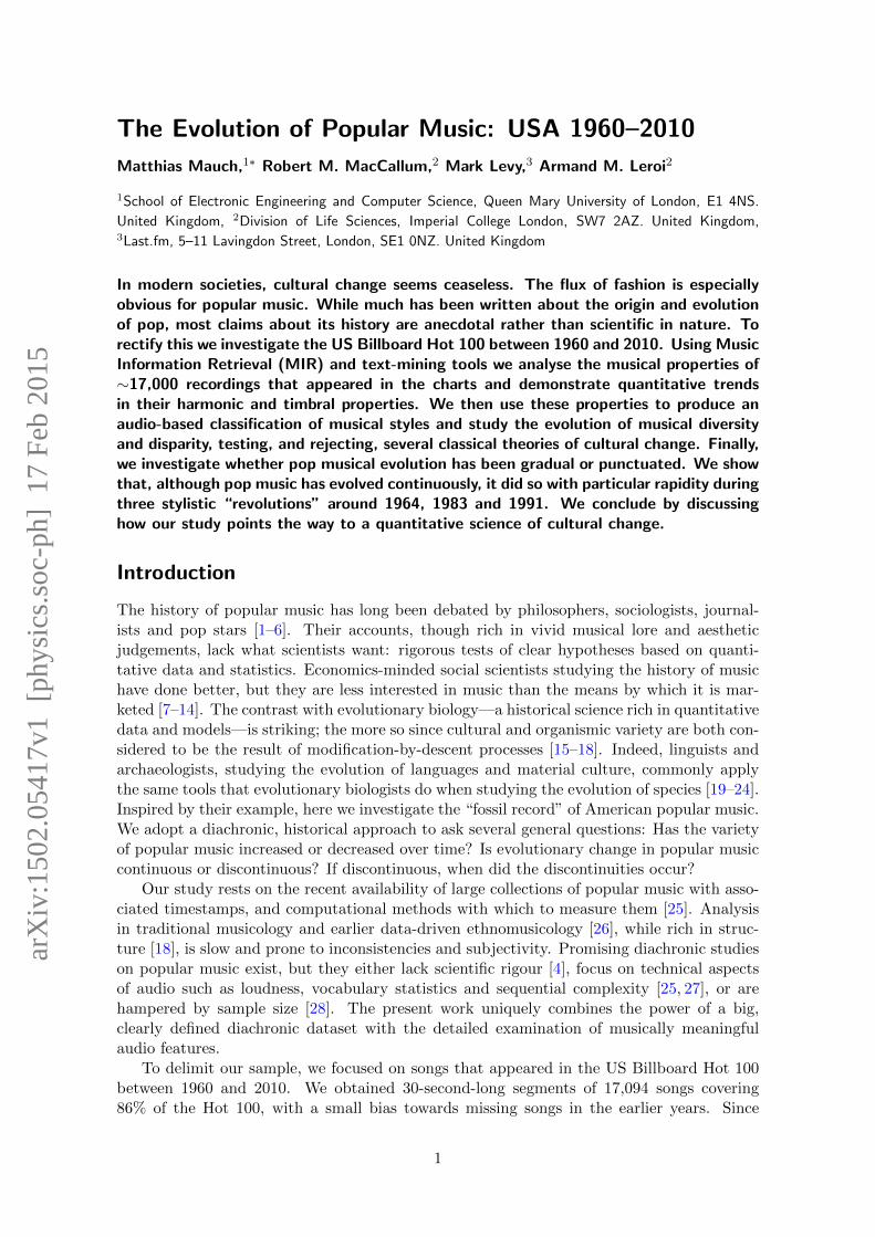
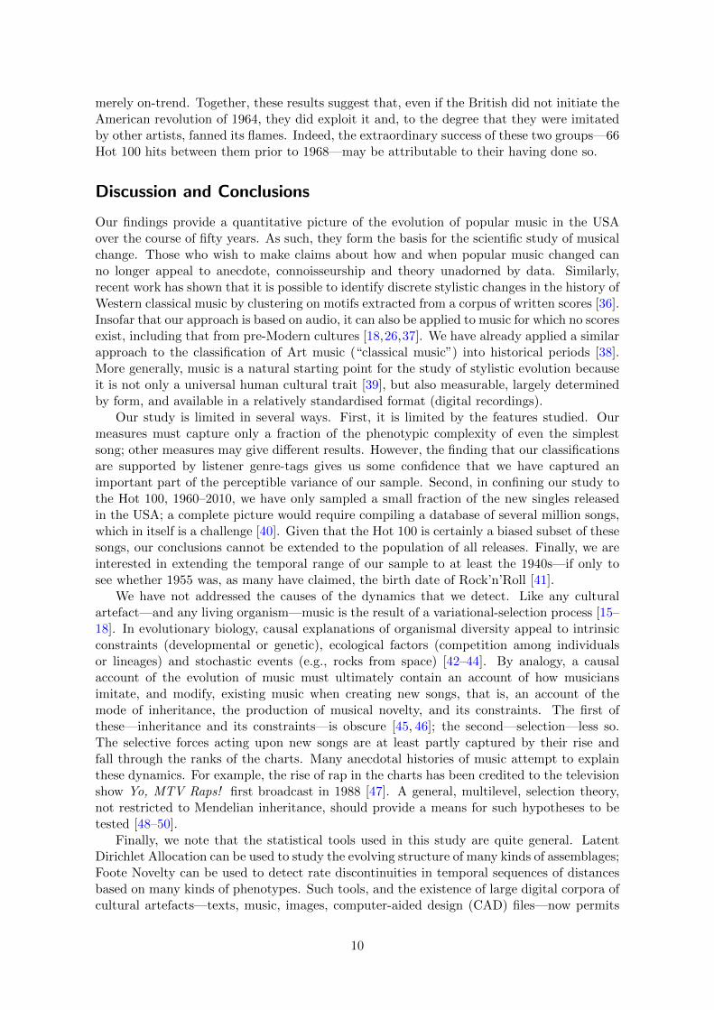
Figure 1: Data processing pipeline illustrated with a segment of Queen’s Bohemian Rhapsody, 1975,one of the few Hot 100 hits to feature an astrophysicist on lead guitar.

1960 1980 2000 1960 1980 2000 1960 1980 2000 1960 1980 2000year

H1 H2 H3 H4 T1 T2 T3 T4

T8T7T6T5H8H7H6H5

0.1

0.2

0.3

0.1

0.2

0.3

qq

dominant 7th chords

natural minor

standard diatonic

major chords, no changes

drums, aggressive, percussive

calm, quiet, mellow

energetic, speech, bright

piano, orchestra, harmonic

guitar, loud, energetic

/ay/, male voice, vocal

/oh/, rounded, mellow

female voice, melodic, vocal

ambiguous tonality

stepwise chord changes

no chords

minor 7th chords

1960 1980 2000 1960 1980 2000 1960 1980 2000 1960 1980 2000year

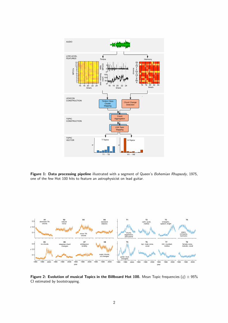
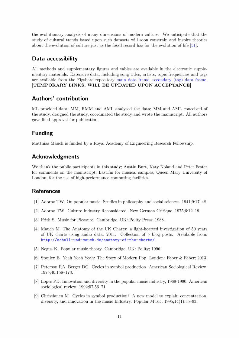
Figure 2: Evolution of musical Topics in the Billboard Hot 100. Mean Topic frequencies (q) ± 95%CI estimated by bootstrapping.

2

our aim is to investigate the evolution of popular taste, we did not attempt to obtain arepresentative sample of all the songs that were released in the USA in that period of time,but just those that were most commercially successful. To analyse the musical propertiesof our songs we adopted an approach inspired by recent advances in text mining (figure 1).We began by measuring our songs for a series of quantitative audio features, 12 descriptorsof tonal content and 14 of timbre (Supplementary Information M.2–3). These were thendiscretised into “words” resulting in a harmonic lexicon (H-lexicon) of chord changes, and atimbral lexicon (T-lexicon) of timbre clusters (SI M.4). To relate the T-lexicon to semanticlabels in plain English we carried out expert annotations (SI M.5). The musical words fromboth lexica were then combined into 8+8=16 “Topics” using Latent Dirichlet Allocation(LDA). LDA is a hierarchical generative model of a text-like corpus, in which every document(here: song) is represented as a distribution over a number of topics, and every topic isrepresented as a distribution over all possible words (here: chord changes from the H-lexicon,and timbre clusters from the T-lexicon). We obtain the most likely model by means ofprobabilistic inference (SI M.6). Each song, then, is represented as a distribution over 8harmonic Topics (H-Topics) that capture classes of chord changes (e.g., “dominant 7th chordchanges”) and 8 timbral Topics (T-Topics) that capture particular timbres (e.g., “drums,aggressive, percussive”, “female voice, melodic, vocal”, derived from the expert annotations),with Topic proportions q. These Topic frequencies were the basis of our analyses.

Results

The Evolution of Topics

Between 1960 and 2010, the frequencies of the Topics in the Hot 100 varied greatly: someTopics became rarer, others became more common, yet others cycled (figure 2). To helpus interpret these dynamics we made use of associations between the Topics and particularartists as well as genre-tags assigned by the listeners of Last.fm, a web-based music discoveryservice with ∼50m users (electronic supplementary material, M.8). Considering the H-Topicsfirst, the most frequent was H8 (mean ± 95%CI: q = 0.236 ± 0.003)—major chords withoutchanges. Nearly two-thirds of our songs show a substantial (> 12.5%) frequency of this Topic,particularly those tagged as classic country, classic rock and love (online tables). Itspresence in the Hot 100 was quite constant, being the most common H-Topic in 43 of 50years.

Other H-Topics were much more dynamic. Between 1960 and 2009 the mean frequency ofH1 declined by about 75%. H1 captures the use of dominant-7th chords. Inherently dissonant(because of the tritone interval between the third and the minor seventh) these chords arecommonly used in Jazz to create tensions that are eventually resolved to consonant chords;in Blues music, the dissonances are typically not resolved and thus add to the characteristic“dirty” colour. Accordingly we find that songs tagged blues or jazz have a high frequencyof H1; it is especially common in the songs of Blues artists such as B.B. King and Jazz artistssuch as Nat “King” Cole. The decline of this Topic, then, represents the lingering death ofJazz and Blues in the Hot 100.

The remaining H-Topics capture the evolution of other musical styles. H3, for example,embraces minor-7th chords used for harmonic colour in funk, disco and soul—this Topic isover-represented in funk and disco and artists like Chic and KC & The Sunshine Band.Between 1967 and 1977, the mean frequency of H3 more than doubles. H6 combines severalchord changes that are a mainstay in modal rock tunes and therefore common in artistswith big-stadium ambitions (e.g., Motley Crue, Van Halen, REO Speedwagon, Queen, Kissand Alice Cooper). Its increase between 1978 and 1985, and subsequent decline in the early

3

1990s, slightly earlier than predicted by the BBC [29], marks the age of Arena Rock. Of allH-Topics, H5 shows the most striking change in frequency. This Topic, which captures theabsence of an identifiable chord structure, barely features in the 1960s and 1970s when, afew spoken-word-music collages aside (e.g., those of Dickie Goodman), nearly all songs hadclearly identifiable chords. H5 starts to become more frequent in the late 1980s and thenrises rapidly to a peak in 1993. This represents the rise of Hip Hop, Rap and related genres,as exemplified by the music of Busta Rhymes, Nas, and Snoop Dog, who all use chordsparticularly rarely (online tables).

The frequencies of the timbral Topics, too, evolve over time. T3, described as “energetic,speech, bright”, shows the same dynamics as H5 and is also associated with the rise of HipHop-related genres. Several of the other timbral Topics, however, appear to rise and fallrepeatedly, suggesting recurring fashions in instrumentation. For example, the evolutionof T4 (“piano, orchestra, harmonic”) appears sinusoidal, suggesting a return in the 2000sto timbral qualities prominent in the 1970s. T5 (“guitar, loud, energetic”) underwent twofull cycles with peaks in 1966 and 1985, heading upward once more in 2009. The second,larger, peak coincides with a peak in H6, the chord-changes also associated with stadium rockgroups such as Motley Crue (online tables). Finally, T1 (“drums, aggressive, percussive”)rises continuously until 1990 which coincides with the spread of new percussive technologysuch as drum machines and the gated reverb effect famously used by Phil Collins on In theair tonight, 1981. Accordingly, T1 is overrepresented in songs tagged dance, disco andnew wave and artists such as The Pet Shop Boys. After 1990, the frequency of T1 declines:the reign of the drum machine was over.

The varieties of music

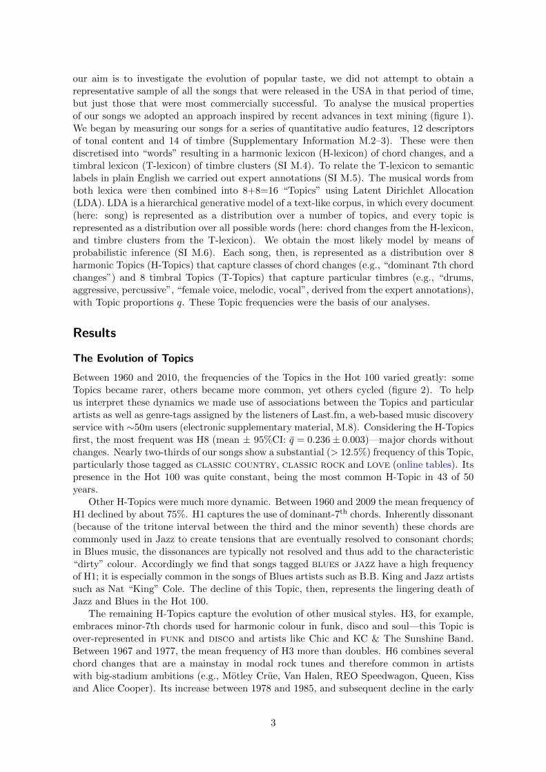
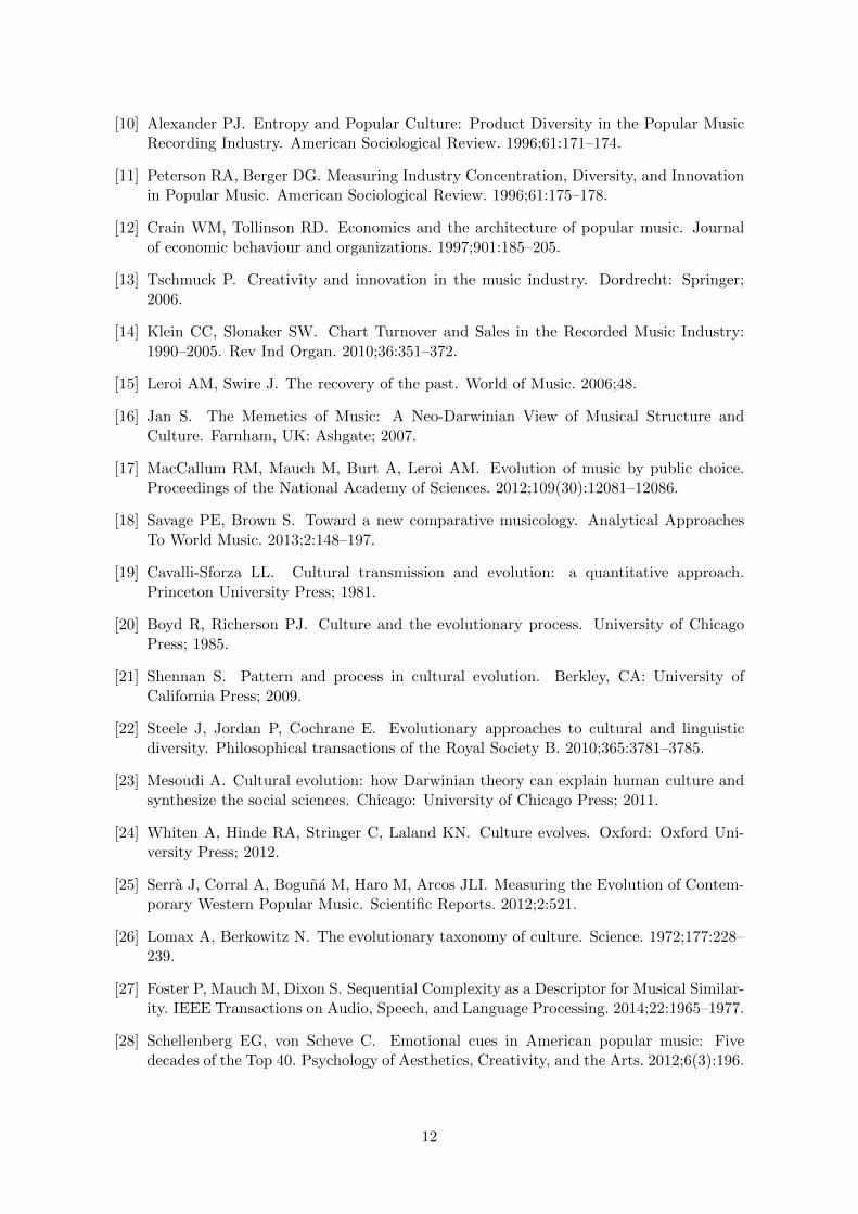
To analyse the evolution of musical variety we began by classifying our songs. Popular musicis classified into genres such as country, rock and roll, rhythm and blues (R’n’B)as well as a multitude of subgenres (dance-pop, synthpop, heartland rock, rootsrock etc.). Such genres are, however, but imperfect reflections of musical qualities. Popularmusic genres such as country and rap partially capture musical styles but, besides beinginformal, are also based on non-musical factors such as the age or ethnicity of performers(e.g., classic rock and K[orean]-Pop) [5]. For this reason we constructed a taxonomy of13 Styles by k-means clustering on principal components derived from our Topic frequencies(figure 3 and electronic supplementary material M.9). We investigated all k < 25 and foundthat the best clustering solution, as determined by mean silhouette score, was k = 13.

In order to relate Last.fm tags to the style Style clusters, we used a technique calledenrichment analysis from bio-informatics. This technique is usually applied to arrive atbiological interpretations of sets of genes, i.e. to find out what the “function” of a set ofgenes is. Applying the GeneMerge enrichment-detection algorithm [30] to our Style data, wefound that all Styles are strongly enriched for particular tags, i.e. for each Style some Last.fmtags are significantly over-represented (table S1), so we conclude that they capture at leastsome of the structure of popular music perceived by consumers. The evolutionary dynamicsof our Styles reflect well-known trends in popular music. For example, the frequency ofStyle 4, strongly enriched for jazz, funk, soul and related tags, declines steadily from 1960onwards. By contrast, Styles 5 and 13, strongly enriched for rock-related tags, fluctuate infrequency, while Style 2, enriched for rap-related tags, is very rare before the mid-1980s butthen rapidly expands to become the single largest Style for the next thirty years, contractingagain in the late 2000s.

What do our Styles represent? Figure 3 shows that Styles and their evolution relateto discrete sub-groups of the charts (genres), and hierarchical cluster analysis suggests thatstyles can be grouped into a higher hierarchy. However, we suppose that, unlike organisms of

4

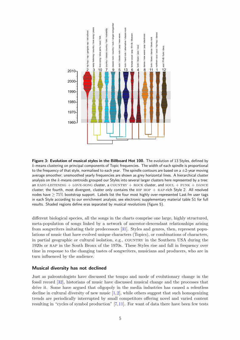
FIGURE 3

hip

hop

/ rap

/ ga

ngst

a ra

p / o

ld s

choo

l

easy

list

enin

g / c

ount

ry /

love

son

g / p

iano

love

-son

g / s

low

jam

s / s

oul /

folk

coun

try /

clas

sic

coun

try /

folk

/ ro

ckab

illy

clas

sic

rock

/ co

untry

/ ro

ck /

sing

er-s

ongw

riter

rock

/ cl

assi

c ro

ck /

pop

/ new

wav

e

rock

/ ha

rd ro

ck /

alte

rnat

ive

/ cla

ssic

-rock

soul

/ R’

nB /

funk

/ di

sco

north

ern

soul

/ so

ul /

hip

hop

/ dan

ce

funk

/ bl

ues

/ dan

ce /

blue

s ro

ck

danc

e / n

ew w

ave

/ pop

/ el

ectro

nic

funk

/ bl

ues

/ jaz

z / s

oul

fem

ale-

voca

l / p

op /

R’n

’B /

Mot

own

1960

1970

1980

1990

2000

2010 12 1110 9 87 65 43 13 12

Figure 3: Evolution of musical styles in the Billboard Hot 100. The evolution of 13 Styles, defined byk-means clustering on principal components of Topic frequencies. The width of each spindle is proportionalto the frequency of that style, normalised to each year. The spindle contours are based on a ±2-year movingaverage smoother; unsmoothed yearly frequencies are shown as grey horizontal lines. A hierarchical clusteranalysis on the k-means centroids grouped our Styles into several larger clusters here represented by a tree:an easy-listening + love-song cluster, a country + rock cluster, and soul + funk + dancecluster; the fourth, most divergent, cluster only contains the hip hop + rap-rich Style 2. All resolvednodes have ≥ 75% bootstrap support. Labels list the four most highly over-represented Last.fm user tagsin each Style according to our enrichment analysis; see electronic supplementary material table S1 for fullresults. Shaded regions define eras separated by musical revolutions (figure 5).

different biological species, all the songs in the charts comprise one large, highly structured,meta-population of songs linked by a network of ancestor-descendant relationships arisingfrom songwriters imitating their predecessors [31]. Styles and genres, then, represent popu-lations of music that have evolved unique characters (Topics), or combinations of characters,in partial geographic or cultural isolation, e.g., country in the Southern USA during the1920s or rap in the South Bronx of the 1970s. These Styles rise and fall in frequency overtime in response to the changing tastes of songwriters, musicians and producers, who are inturn influenced by the audience.

Musical diversity has not declined

Just as paleontologists have discussed the tempo and mode of evolutionary change in thefossil record [32], historians of music have discussed musical change and the processes thatdrive it. Some have argued that oligopoly in the media industries has caused a relentlessdecline in cultural diversity of new music [1,2], while others suggest that such homogenizingtrends are periodically interrupted by small competitors offering novel and varied contentresulting in “cycles of symbol production” [7,11]. For want of data there have been few tests

5

200 400

●●

●●

●●●●

●●

●●

●●

●●

●●●●

●●

●●

●●●

●●●

●●●●●●

●●●

●●●●●●●

●●

●●

DN

FIGURE 4

600

●●

●●

●●●

●●

●●

●●

●●

●●

●●

●●

●●

●●

●●

●●

●●

●●

●●●

●●

●●

●●

●●

●●

●●

●●

9 10 11 12D

S

●●●

●●●

●●

●●

●●

●●

●●

●●

●●

●●

●●

●●●

●●

●●

●●

●●●

●●●

●●●●

●●

●●●

●●

DT

6.8 7.2 7.6

●●

●●

●●●

●●

●●●

●●

●●

●●

●●

●●

●●

●●●

●●

●●●

●●

●●

●●●●

●●●

●●

●●

●●

●

-2 0 2D

Y

1960

1970

1980

1990

2000

2010

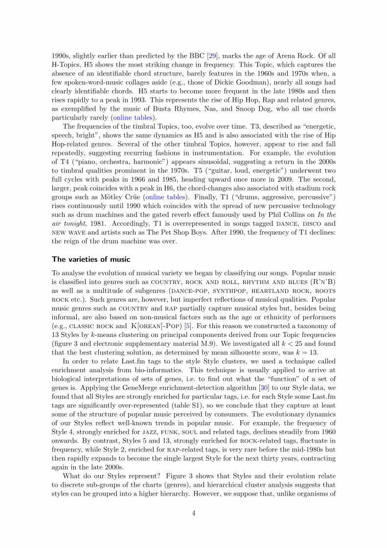
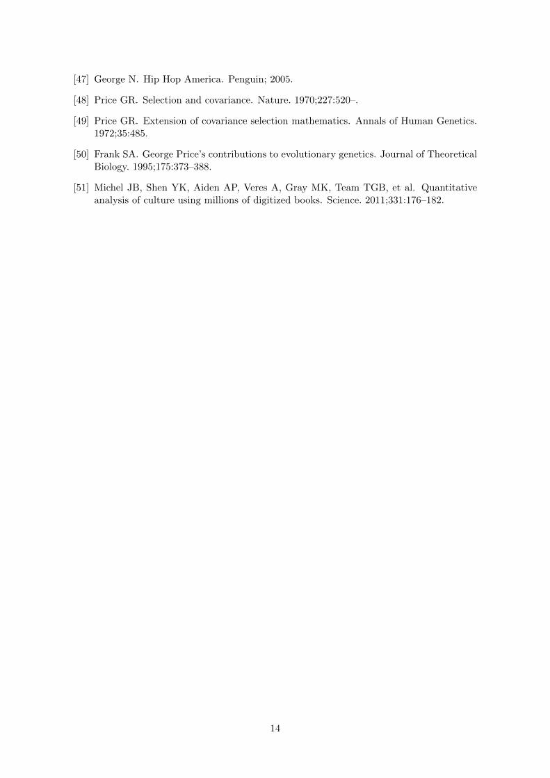
Figure 4: Evolution of musical diversity in the Billboard Hot 100. We estimate four measures ofdiversity. From left to right: Song number in the charts, DN, depends only on the rate of turnover ofunique entities (songs), and takes no account of their phenotypic similarity. Class diversity, DS, is theeffective number of Styles and captures functional diversity. Topic diversity, DT, is the effective numberof musical Topics used each year, averaged across the Harmonic and Timbral Topics. Disparity, DY, orphenotypic range is estimated as the total standard deviation within a year. Note that although in ecologyDS and DY are often applied to sets of distinct species or lineages they need not be; our use of themimplies nothing about the ontological status of our Styles and Topics. For full definitions of the diversitymeasures see electronic supplementary material, M.11. Shaded regions define eras separated by musicalrevolutions (figure 5).

of either theory [8–10,13].To test these ideas we estimated four yearly measures of diversity (figure 4). We found

that although all four evolve, two—Topic diversity and disparity—show the most strikingchanges, both declining to a minimum around 1984, but then rebounding and increasingto a maximum in the early 2000s. Since neither of these measures track song number,their dynamics cannot be due to varying numbers of songs in the Hot 100; nor, since oursampling over 50 years is nearly complete, can they be due to the over-representation ofrecent songs—the so-called “pull of the recent” [33]. Instead, their dynamics are due tochanges in the frequencies of musical styles.

The decline in Topic diversity and disparity in the early 1980s is due to a decline oftimbral rather than harmonic diversity (electronic supplementary material, figure S1). Thiscan be seen in the evolution of particular topics (figure 2). In the early 1980s timbral Top-ics T1 (drums, aggressive, percussive) and T5 (guitar, loud, energetic) become increasinglydominant; the subsequent recovery of diversity is due to the relative decrease in frequencyof the these topics as T3 (energetic, speech, bright) increases. Put in terms of Styles, thedecline of diversity is due to the dominance of genres such as new wave, disco, hardrock;its recovery is due to their waning with the rise of rap and related genres (figure 2). Con-trary to current theories of musical evolution, then, we find no evidence for the progressivehomogenisation of music in the charts and little sign of diversity cycles within the 50 yeartime frame of our study. Instead, the evolution of chart diversity is dominated by historicallyunique events: the rise and fall of particular ways of making music.

Musical evolution is punctuated by revolutions

The history of popular music is often seen as a succession of distinct eras, e.g., the “RockEra”, separated by revolutions [3,6,13]. Against this, some scholars have argued that musicaleras and revolutions are illusory [5]. Even among those who see discontinuities, there is little

6

B

0.05

0.001

1960 1970 1980 1990 2000 2010

1960

1970

1980

1990

2000

2010A

0.01

year

s

1960 1970 1980 1990 2000 2010

12

510

kern

el h

alf-w

idth

(ye

ars)

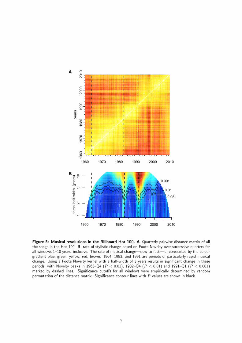
Figure 5: Musical revolutions in the Billboard Hot 100. A. Quarterly pairwise distance matrix of allthe songs in the Hot 100. B. rate of stylistic change based on Foote Novelty over successive quarters forall windows 1–10 years, inclusive. The rate of musical change—slow-to-fast—is represented by the colourgradient blue, green, yellow, red, brown: 1964, 1983, and 1991 are periods of particularly rapid musicalchange. Using a Foote Novelty kernel with a half-width of 3 years results in significant change in theseperiods, with Novelty peaks in 1963–Q4 (P < 0.01), 1982–Q4 (P < 0.01) and 1991–Q1 (P < 0.001)marked by dashed lines. Significance cutoffs for all windows were empirically determined by randompermutation of the distance matrix. Significance contour lines with P values are shown in black.

7

agreement about when they occurred. The problem, again, is that data have been scarceand objective criteria for deciding what constitutes a break in a historical sequence, scarceryet.

To determine directly whether rate discontinuities exist we divided the period 1960–2010into 200 quarters and used the principal components of the Topic frequencies to estimate apairwise distance matrix between them (figure 5A). This matrix suggested that, while musicalevolution was ceaseless, there were periods of relative stasis punctuated by periods of rapidchange. To test this impression we applied a method from Music Information Retrieval,Foote Novelty, which estimates the magnitude of change in a distance matrix over a giventemporal window [34]. The method relies on a kernel matrix with a checkerboard pattern.Since a distance matrix exposes just such a checkerboard pattern at change points [34],convolving it with the checkerboard kernel along its diagonal directly yields the noveltyfunction (SI M.11). We calculated Foote Novelty for all windows between 1 and 10 years and,for each window, determined empirical significance cutoffs based on random permutation ofthe distance matrix. We identified three revolutions: a major one around 1991 and twosmaller ones around 1964 and 1983 (figure 5B). From peak to succeeding trough, the rate ofmusical change during these revolutions varied 4- to 6-fold.

This temporal analysis, when combined with our Style clusters (figure 3), shows howmusical revolutions are associated with the expansion and contraction of particular musicalstyles. Using quadratic regression models, we identified the Styles that showed significant(P < 0.01) change in frequency against time in the six years surrounding each revolu-tion (electronic supplementary material, table S2). We also carried out a Style-enrichmentanalysis for the same periods (electronic supplementary material, table S2). Of the threerevolutions 1964 was the most complex, involving the expansion of several Styles—1, 5, 8,12 and 13—enriched at the time for soul and rock-related tags. These gains were boughtat the expense of Styles 3 and 6 both enriched for doowop among other tags. The 1983revolution is associated with an expansion of three Styles—8,11 and 13—here enriched fornew wave, disco and hard rock-related tags and the contraction of three Styles—3, 7and 12—here enriched for soft rock, country-related or soul + r’n’b-related tags. Thelargest revolution of the three, 1991, is associated with the expansion of Style 2, enrichedfor rap-related tags, at the expense of Styles 5 and 13, here enriched for rock-related tags.The rise of rap and related genres appears, then, to be the single most important event thathas shaped the musical structure of the American charts in the period that we studied.

The British did not start the American revolution of ’64

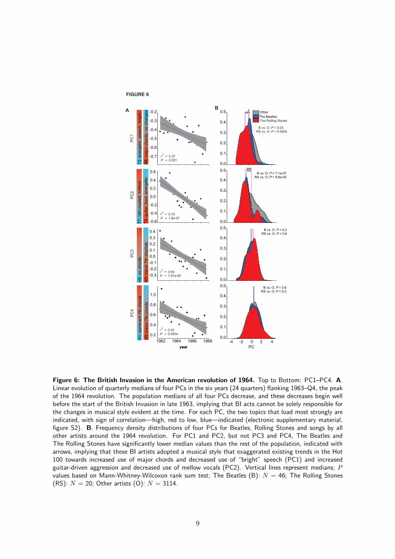
Our analysis does not reveal the origins of musical styles; rather, it shows when changes instyle frequency affect the musical structure of the charts. Bearing this in mind we investigatedthe roles of particular artists in one revolution. On 26 December, 1963, The Beatles released Iwant to hold your hand in the USA. They were swiftly followed by dozens of British acts who,over the next few years, flooded the American charts. It is often claimed that this “BritishInvasion” (BI) was responsible for musical changes of the time [35]. Was it? As noted above,around 1964 many Styles were changing in frequency; many principal components of theTopic frequencies show linear changes in this period too. Inspection of the first four PCsshows that their evolutionary trajectories were all established before 1964, implying that,while the British may have contributed to this revolution, they could not have been entirelyresponsible for it (figure 6A). We then compared two of the most successful BI acts, TheBeatles and The Rolling Stones, to the rest of the Hot 100 (figure 6B). In the case of PC1and PC2, the songs of both bands have (low) values that anticipate the Hot 100’s trajectory:for these musical attributes they were literally ahead of the curve. In the case of PC3 andPC4 their songs resemble the rest of the Hot 100: for these musical attributes they were

8

-0.7

-0.6

-0.5

-0.4

-0.3

-0.2

-0.6

-0.4

-0.2

0.0

0.2

0.4

0.6

-0.3

-0.2

-0.1

0.0

0.1

0.2

0.3

0.4

0.2

0.4

0.6

0.8

1.0

1962 1964 1966 1968

year

0.0

0.1

0.2

0.3

0.4

0.5

0.0

0.1

0.2

0.3

0.4

0.5

0.0

0.1

0.2

0.3

0.4

0.5

0.0

0.1

0.2

0.3

0.4

0.5

-4 -2 0 2 4

OtherThe BeatlesThe Rolling Stones

year

PC

1P

C2

PC

3P

C4

PC

FIGURE 6

r2

=P =

0.370.001

r2

=P =

0.701.8e-07

r2

=P =

0.501.91e-05

r2

=P =

0.420.0004

B vs. O: P = 0.03RS vs. O: P = 0.0004

B vs. O: P = 7.1e-07RS vs. O: P = 8.9e-05

B vs. O: P = 0.2RS vs. O: P = 0.6

B vs. O: P = 0.8RS vs. O: P = 0.5

A B

T4

H8:

maj

or c

hord

s, n

o ch

ange

s

T3:

ene

rget

ic, s

peec

h, b

right

T5:

gui

tar,

loud

, ene

rget

ic

T7:

/oh/

,rou

ded,

mel

low

H3:

min

or 7

th c

horh

ds

H5:

no

chor

ds

H3:

min

or 7

th c

hord

s

H1:

dom

inan

t 7th

cho

rds

******

****

Figure 6: The British Invasion in the American revolution of 1964. Top to Bottom: PC1–PC4. A.Linear evolution of quarterly medians of four PCs in the six years (24 quarters) flanking 1963–Q4, the peakof the 1964 revolution. The population medians of all four PCs decrease, and these decreases begin wellbefore the start of the British Invasion in late 1963, implying that BI acts cannot be solely responsible forthe changes in musical style evident at the time. For each PC, the two topics that load most strongly areindicated, with sign of correlation—high, red to low, blue—indicated (electronic supplementary material,figure S2). B. Frequency density distributions of four PCs for Beatles, Rolling Stones and songs by allother artists around the 1964 revolution. For PC1 and PC2, but not PC3 and PC4, The Beatles andThe Rolling Stones have significantly lower median values than the rest of the population, indicated witharrows, implying that these BI artists adopted a musical style that exaggerated existing trends in the Hot100 towards increased use of major chords and decreased use of “bright” speech (PC1) and increasedguitar-driven aggression and decreased use of mellow vocals (PC2). Vertical lines represent medians; Pvalues based on Mann-Whitney-Wilcoxon rank sum test; The Beatles (B): N = 46; The Rolling Stones(RS): N = 20; Other artists (O): N = 3114.

9

merely on-trend. Together, these results suggest that, even if the British did not initiate theAmerican revolution of 1964, they did exploit it and, to the degree that they were imitatedby other artists, fanned its flames. Indeed, the extraordinary success of these two groups—66Hot 100 hits between them prior to 1968—may be attributable to their having done so.

Discussion and Conclusions

Our findings provide a quantitative picture of the evolution of popular music in the USAover the course of fifty years. As such, they form the basis for the scientific study of musicalchange. Those who wish to make claims about how and when popular music changed canno longer appeal to anecdote, connoisseurship and theory unadorned by data. Similarly,recent work has shown that it is possible to identify discrete stylistic changes in the history ofWestern classical music by clustering on motifs extracted from a corpus of written scores [36].Insofar that our approach is based on audio, it can also be applied to music for which no scoresexist, including that from pre-Modern cultures [18,26,37]. We have already applied a similarapproach to the classification of Art music (“classical music”) into historical periods [38].More generally, music is a natural starting point for the study of stylistic evolution becauseit is not only a universal human cultural trait [39], but also measurable, largely determinedby form, and available in a relatively standardised format (digital recordings).

Our study is limited in several ways. First, it is limited by the features studied. Ourmeasures must capture only a fraction of the phenotypic complexity of even the simplestsong; other measures may give different results. However, the finding that our classificationsare supported by listener genre-tags gives us some confidence that we have captured animportant part of the perceptible variance of our sample. Second, in confining our study tothe Hot 100, 1960–2010, we have only sampled a small fraction of the new singles releasedin the USA; a complete picture would require compiling a database of several million songs,which in itself is a challenge [40]. Given that the Hot 100 is certainly a biased subset of thesesongs, our conclusions cannot be extended to the population of all releases. Finally, we areinterested in extending the temporal range of our sample to at least the 1940s—if only tosee whether 1955 was, as many have claimed, the birth date of Rock’n’Roll [41].

We have not addressed the causes of the dynamics that we detect. Like any culturalartefact—and any living organism—music is the result of a variational-selection process [15–18]. In evolutionary biology, causal explanations of organismal diversity appeal to intrinsicconstraints (developmental or genetic), ecological factors (competition among individualsor lineages) and stochastic events (e.g., rocks from space) [42–44]. By analogy, a causalaccount of the evolution of music must ultimately contain an account of how musiciansimitate, and modify, existing music when creating new songs, that is, an account of themode of inheritance, the production of musical novelty, and its constraints. The first ofthese—inheritance and its constraints—is obscure [45, 46]; the second—selection—less so.The selective forces acting upon new songs are at least partly captured by their rise andfall through the ranks of the charts. Many anecdotal histories of music attempt to explainthese dynamics. For example, the rise of rap in the charts has been credited to the televisionshow Yo, MTV Raps! first broadcast in 1988 [47]. A general, multilevel, selection theory,not restricted to Mendelian inheritance, should provide a means for such hypotheses to betested [48–50].

Finally, we note that the statistical tools used in this study are quite general. LatentDirichlet Allocation can be used to study the evolving structure of many kinds of assemblages;Foote Novelty can be used to detect rate discontinuities in temporal sequences of distancesbased on many kinds of phenotypes. Such tools, and the existence of large digital corpora ofcultural artefacts—texts, music, images, computer-aided design (CAD) files—now permits

10

the evolutionary analysis of many dimensions of modern culture. We anticipate that thestudy of cultural trends based upon such datasets will soon constrain and inspire theoriesabout the evolution of culture just as the fossil record has for the evolution of life [51].

Data accessibility

All methods and supplementary figures and tables are available in the electronic supple-mentary materials. Extensive data, including song titles, artists, topic frequencies and tagsare available from the Figshare repository main data frame, secondary (tag) data frame.[TEMPORARY LINKS, WILL BE UPDATED UPON ACCEPTANCE]

Authors’ contribution

ML provided data; MM, RMM and AML analysed the data; MM and AML conceived ofthe study, designed the study, coordinated the study and wrote the manuscript. All authorsgave final approval for publication.

Funding

Matthias Mauch is funded by a Royal Academy of Engineering Research Fellowship.

Acknowledgments

We thank the public participants in this study; Austin Burt, Katy Noland and Peter Fosterfor comments on the manuscript; Last.fm for musical samples; Queen Mary University ofLondon, for the use of high-performance computing facilities.

References

[1] Adorno TW. On popular music. Studies in philosophy and social sciences. 1941;9:17–48.

[2] Adorno TW. Culture Industry Reconsidered. New German Critique. 1975;6:12–19.

[3] Frith S. Music for Pleasure. Cambridge, UK: Polity Press; 1988.

[4] Mauch M. The Anatomy of the UK Charts: a light-hearted investigation of 50 yearsof UK charts using audio data; 2011. Collection of 5 blog posts. Available from:http://schall-und-mauch.de/anatomy-of-the-charts/.

[5] Negus K. Popular music theory. Cambridge, UK: Polity; 1996.

[6] Stanley B. Yeah Yeah Yeah: The Story of Modern Pop. London: Faber & Faber; 2013.

[7] Peterson RA, Berger DG. Cycles in symbol production. American Sociological Review.1975;40:158–173.

[8] Lopes PD. Innovation and diversity in the popular music industry, 1969-1990. Americansociological review. 1992;57:56–71.

[9] Christianen M. Cycles in symbol production? A new model to explain concentration,diversity, and innovation in the music Industry. Popular Music. 1995;14(1):55–93.

11

[10] Alexander PJ. Entropy and Popular Culture: Product Diversity in the Popular MusicRecording Industry. American Sociological Review. 1996;61:171–174.

[11] Peterson RA, Berger DG. Measuring Industry Concentration, Diversity, and Innovationin Popular Music. American Sociological Review. 1996;61:175–178.

[12] Crain WM, Tollinson RD. Economics and the architecture of popular music. Journalof economic behaviour and organizations. 1997;901:185–205.

[13] Tschmuck P. Creativity and innovation in the music industry. Dordrecht: Springer;2006.

[14] Klein CC, Slonaker SW. Chart Turnover and Sales in the Recorded Music Industry:1990–2005. Rev Ind Organ. 2010;36:351–372.

[15] Leroi AM, Swire J. The recovery of the past. World of Music. 2006;48.

[16] Jan S. The Memetics of Music: A Neo-Darwinian View of Musical Structure andCulture. Farnham, UK: Ashgate; 2007.

[17] MacCallum RM, Mauch M, Burt A, Leroi AM. Evolution of music by public choice.Proceedings of the National Academy of Sciences. 2012;109(30):12081–12086.

[18] Savage PE, Brown S. Toward a new comparative musicology. Analytical ApproachesTo World Music. 2013;2:148–197.

[19] Cavalli-Sforza LL. Cultural transmission and evolution: a quantitative approach.Princeton University Press; 1981.

[20] Boyd R, Richerson PJ. Culture and the evolutionary process. University of ChicagoPress; 1985.

[21] Shennan S. Pattern and process in cultural evolution. Berkley, CA: University ofCalifornia Press; 2009.

[22] Steele J, Jordan P, Cochrane E. Evolutionary approaches to cultural and linguisticdiversity. Philosophical transactions of the Royal Society B. 2010;365:3781–3785.

[23] Mesoudi A. Cultural evolution: how Darwinian theory can explain human culture andsynthesize the social sciences. Chicago: University of Chicago Press; 2011.

[24] Whiten A, Hinde RA, Stringer C, Laland KN. Culture evolves. Oxford: Oxford Uni-versity Press; 2012.

[25] Serra J, Corral A, Boguna M, Haro M, Arcos JLI. Measuring the Evolution of Contem-porary Western Popular Music. Scientific Reports. 2012;2:521.

[26] Lomax A, Berkowitz N. The evolutionary taxonomy of culture. Science. 1972;177:228–239.

[27] Foster P, Mauch M, Dixon S. Sequential Complexity as a Descriptor for Musical Similar-ity. IEEE Transactions on Audio, Speech, and Language Processing. 2014;22:1965–1977.

[28] Schellenberg EG, von Scheve C. Emotional cues in American popular music: Fivedecades of the Top 40. Psychology of Aesthetics, Creativity, and the Arts. 2012;6(3):196.

12

[29] Barfield S. Seven Ages of Rock: We Are The Champions. BBC; 2007.Accessed: 2015-01-16. http://www.bbc.co.uk/music/sevenages/programmes/

we-are-the-champions/.

[30] Castillo-Davis CI, Hartl DL. GeneMerge – post genomic analysis, data mining, andhypothesis testing. Bioinformatics. 2003;19:891–892.

[31] Zollo P. Songwriters on songwriting. Da Capo Press; 2003.

[32] Simpson GG. Tempo and mode in evolution. Columbia University Press; 1944.

[33] Jablonski D, Roy K, Valentine JW, Price RM, Anderson PS. The impact of the Pull ofthe Recent on the history of bivalve diversity. Science. 2003;300:1133–1135.

[34] Foote J. Automatic audio segmentation using a measure of audio novelty. In: IEEEInternational Conference on Multimedia and Expo. vol. 1; 2000. p. 452–455.

[35] Fitzgerald J. When the Brill building met Lennon-McCartney: Continuity and change inthe early evolution of the mainstream pop song. Popular Music & Society. 1995;19(1):59–77.

[36] Rodriguez Zivica PH, Shifresb F, Cecchic GA. Perceptual basis of evolving Westernmusical styles. Proceedings of the National Academy of Sciences, USA. 2013;110:10034–10038.

[37] Lomax A. Folk song style and culture. Washington, D. C.: American Association forthe Advancement of Science; 1968.

[38] Weiß C, Mauch M, Dixon S. Timbre-invariant Audio Features for Style Analysis ofClassical Music. In: Proceedings of the 11th Music Computing Conference (SMC 2014);2014. p. 1461–1468.

[39] Brown DE. Human universals. Temple University Press, Philadelphia; 1991. Pp. 1–160.

[40] Bertin-Mahieux T, Ellis DPW, Whitman B, Lamere P. The million song dataset. In:Proceedings of the 12th International Society for Music Information Retrieval Confer-ence (ISMIR 2011); 2011. p. 591–596.

[41] Peterson RA. Why 1955? Explaining the Advent of Rock Music. Popular Music.1990;9:97–116.

[42] Erwin DH. DISPARITY: MORPHOLOGICAL PATTERN AND DEVELOPMENTALCONTEXT. Palaeontology. 2007;50(1):57–73.

[43] Gould SJ. The Structure of Evolutionary Theory. Cambridge, MA: Harvard UniversityPress; 2002.

[44] Jablonski D. Species selection: Theory and data. Annual Review of Ecology andSystmatics. 2008;39(501-524).

[45] Pachet F. Creativity studies and musical interaction. In: Deliege I, Wiggins GA,editors. Musical Creativity: Multidisciplinary Research in Theory and Practice. Hove,UK: Psychology Press; 2006. p. 347–358.

[46] McIntyre P. Creativity and cultural production: a study of contemporary Westernpopular music songwriting. Creativity Research Journal. 2008;20(1):40–52.

13

[47] George N. Hip Hop America. Penguin; 2005.

[48] Price GR. Selection and covariance. Nature. 1970;227:520–.

[49] Price GR. Extension of covariance selection mathematics. Annals of Human Genetics.1972;35:485.

[50] Frank SA. George Price’s contributions to evolutionary genetics. Journal of TheoreticalBiology. 1995;175:373–388.

[51] Michel JB, Shen YK, Aiden AP, Veres A, Gray MK, Team TGB, et al. Quantitativeanalysis of culture using millions of digitized books. Science. 2011;331:176–182.

14

The evolution of popular music: USA 1960-2010:

Supporting Information

Matthias Mauch, Robert M. MacCallum, Mark Levy, Armand M. Leroi

15 October, 2014

Contents

M Materials and Methods 2M.1 The origin of the songs . . . . . . . . . . . . . . . . . . . . . . . . . . . . . . . . . . . 2M.2 Measuring Harmony. . . . . . . . . . . . . . . . . . . . . . . . . . . . . . . . . . . . . 2M.3 Measuring Timbre. . . . . . . . . . . . . . . . . . . . . . . . . . . . . . . . . . . . . . 3M.4 Making musical lexica . . . . . . . . . . . . . . . . . . . . . . . . . . . . . . . . . . . . 3M.5 Semantic lexicon annotation . . . . . . . . . . . . . . . . . . . . . . . . . . . . . . . . 4M.6 Topic extraction . . . . . . . . . . . . . . . . . . . . . . . . . . . . . . . . . . . . . . . 5M.7 Semantic topic annotations . . . . . . . . . . . . . . . . . . . . . . . . . . . . . . . . . 6M.8 User-generated tags . . . . . . . . . . . . . . . . . . . . . . . . . . . . . . . . . . . . . 7M.9 Identifying musical Styles clusters: k-means and silhouette scores . . . . . . . . . . . 7M.10 Diversity metrics . . . . . . . . . . . . . . . . . . . . . . . . . . . . . . . . . . . . . . 8M.11 Identifying musical revolutions . . . . . . . . . . . . . . . . . . . . . . . . . . . . . . . 9M.12 Identifying Styles that change around each revolution . . . . . . . . . . . . . . . . . . 10

S Supplementary Text & Tables 11

1

M Materials and Methods

M.1 The origin of the songs

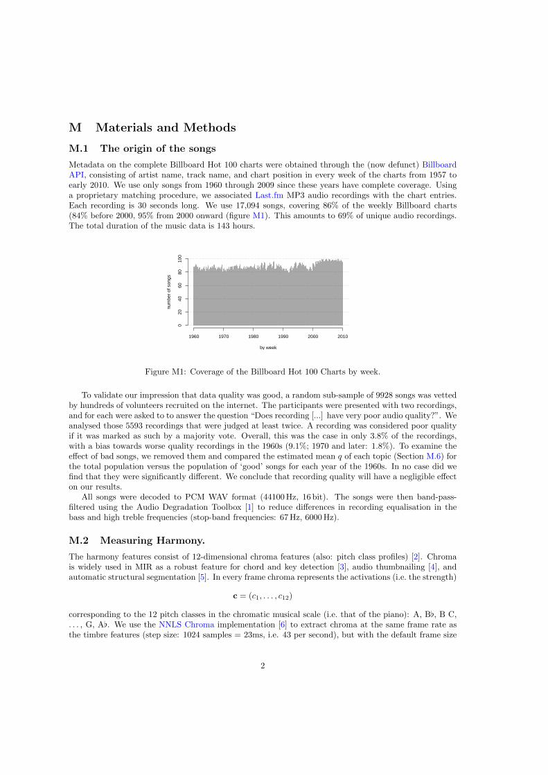
Metadata on the complete Billboard Hot 100 charts were obtained through the (now defunct) BillboardAPI, consisting of artist name, track name, and chart position in every week of the charts from 1957 toearly 2010. We use only songs from 1960 through 2009 since these years have complete coverage. Usinga proprietary matching procedure, we associated Last.fm MP3 audio recordings with the chart entries.Each recording is 30 seconds long. We use 17,094 songs, covering 86% of the weekly Billboard charts(84% before 2000, 95% from 2000 onward (figure M1). This amounts to 69% of unique audio recordings.The total duration of the music data is 143 hours.

1960 1970 1980 1990 2000 2010

020

4060

8010

0

by week

num

ber

of s

ongs

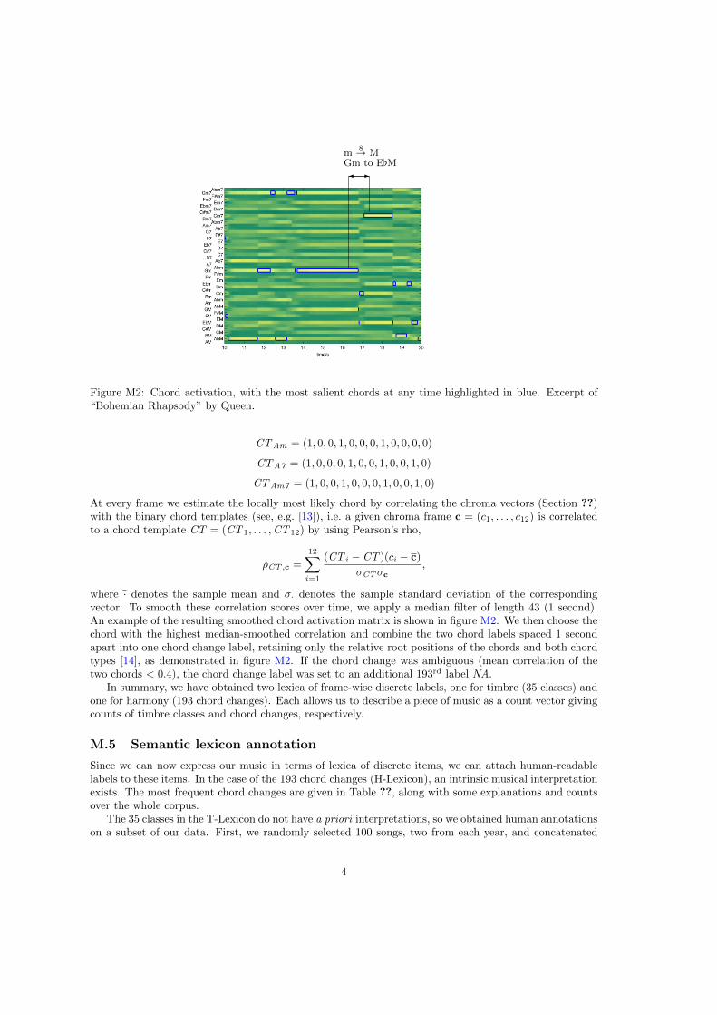
Figure M1: Coverage of the Billboard Hot 100 Charts by week.

To validate our impression that data quality was good, a random sub-sample of 9928 songs was vettedby hundreds of volunteers recruited on the internet. The participants were presented with two recordings,and for each were asked to to answer the question “Does recording [...] have very poor audio quality?”. Weanalysed those 5593 recordings that were judged at least twice. A recording was considered poor qualityif it was marked as such by a majority vote. Overall, this was the case in only 3.8% of the recordings,with a bias towards worse quality recordings in the 1960s (9.1%; 1970 and later: 1.8%). To examine theeffect of bad songs, we removed them and compared the estimated mean q of each topic (Section M.6) forthe total population versus the population of ‘good’ songs for each year of the 1960s. In no case did wefind that they were significantly different. We conclude that recording quality will have a negligible effecton our results.

All songs were decoded to PCM WAV format (44100 Hz, 16 bit). The songs were then band-pass-filtered using the Audio Degradation Toolbox [1] to reduce differences in recording equalisation in thebass and high treble frequencies (stop-band frequencies: 67 Hz, 6000 Hz).

M.2 Measuring Harmony.

The harmony features consist of 12-dimensional chroma features (also: pitch class profiles) [2]. Chromais widely used in MIR as a robust feature for chord and key detection [3], audio thumbnailing [4], andautomatic structural segmentation [5]. In every frame chroma represents the activations (i.e. the strength)

c = (c1, . . . , c12)

corresponding to the 12 pitch classes in the chromatic musical scale (i.e. that of the piano): A, B[, B C,. . . , G, A[. We use the NNLS Chroma implementation [6] to extract chroma at the same frame rate asthe timbre features (step size: 1024 samples = 23ms, i.e. 43 per second), but with the default frame size

2

of 16384 samples. The chroma representation (often called chromagram) of the complete 30 s excerpt of“Bohemian Rhapsody” is shown in figure 1 (main text).

M.3 Measuring Timbre.

The timbre features consist of 12 Mel-frequency cepstral coefficients (MFCCs), one delta-MFCC value, andone Zero-crossing Count (ZCC) feature. MFCCs are spectral-domain audio features for the descriptionof timbre and are routinely used in speech recognition [7] and Music Information Retrieval (MIR) tasks[8]. For every frame, they provide a low-dimensional parametrisation of the overall shape of the signal’sMel-spectrum, i.e. a spectral representation that takes into account human near-logarithmic perceptionof sound in magnitude (log-magnitude) and frequency (Mel scale). We use the first 12 MFCCs (excludingthe 0th component) and additionally one delta-MFCC, calculated as the difference between any twoconsecutive values of the 0th MFCC component. The MFCCs were extracted using a plugin from theVamp library (seen 27.03.2014) with the default parameters (block size: 2048 samples = 46ms, stepsize: 1024 samples = 23ms). This amounts to ≈ 43 frames per second. The ZCC (also: zero-crossingrate, ZCR) is a time-domain audio feature which has been used in speech recognition [9] and has beenapplied successfully to discern drum sounds [10]. It is calculated by simply counting the number of timesconsecutive samples in a frame are of opposite sign. ZCC is high for noisy signals and transient sounds atthe onset of consonants and percussive events. To extract the ZCC we also used a Vamp plugin, extractingfeatures at the same frame rate (43 per second, step size: 1024 sampes = 23ms), but with a block sizeof 1024 samples. MFCCs and zero crossing counts of “Bohemian Rhapsody” are shown in figure 1 (maintext).

M.4 Making musical lexica

Since we aim to apply topic models to our data (see Section M.6), we need to discretise our raw featuresinto musical lexica. We have one timbral lexicon (T-Lexicon) and one harmonic lexicon (H-Lexicon).

Timbre.

In order to define the T-Lexicon we followed an unsupervised feature learning approach by quantisingthe feature space into 35 discrete classes as follows. First, we randomly selected 20 frames from eachof 11350 randomly selected songs (227 from every year), a total of 227,000 frames. The features werethen standardised, and de-correlated using principal component analysis (PCA). The PCA componentswere once more standardised. We then applied model-based clustering (Gaussian mixture models, GMM)to the standardised de-correlated data, using the built-in Matlab function gmdistribution.fit with fullcovariance matrix [11]. The GMM with 35 mixtures (clusers) was chosen as it minimised the BayesInformation Criterion. We then transformed all songs according to the same PCA, scaling and clustermapping transformations. In particular, every audio frame was assigned to its most likely cluster accordingto the GMM. Frames with cluster probabilities of < 0.5 were removed.

Harmony.

Our H-Lexicon consists of all 192 possible changes between the most frequently used chord types inpopular music [12]: major (M), minor (m), dominant 7 (7) and minor 7 chords (m7). We use chordchanges because they offer a key-independent way of describing the temporal dynamics of harmony. As achord is defined by its root pitch class (A,Bb,B,C,. . . ,Ab[) and its type, our system gives rise to 4×12 = 48chords. Each of the chords can be represented as a binary chord template with 12 elements correspondingto the twelve pitch classes. For example, the four chords with root A are these.

CTAM = (1, 0, 0, 0, 1, 0, 0, 1, 0, 0, 0, 0)

3

-�

m8→ M

Gm to E[M

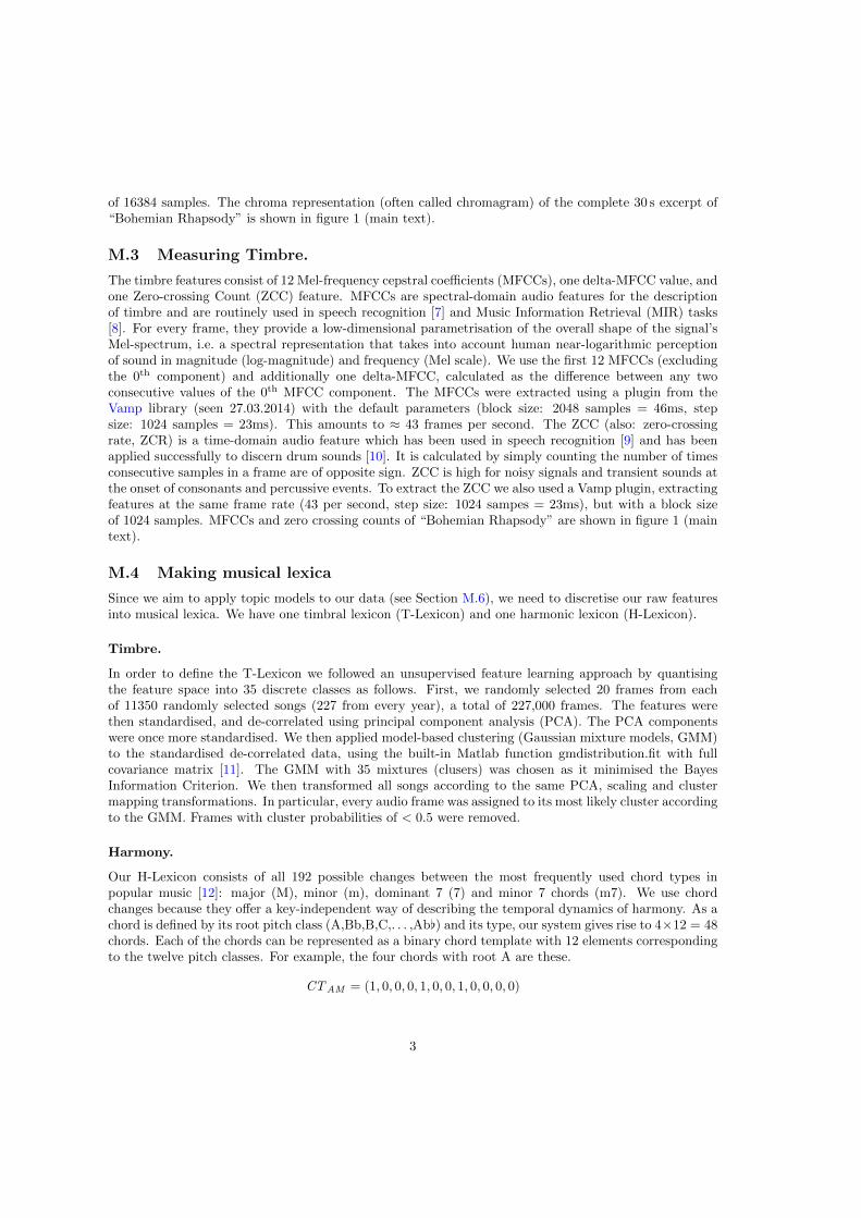
Figure M2: Chord activation, with the most salient chords at any time highlighted in blue. Excerpt of“Bohemian Rhapsody” by Queen.

CTAm = (1, 0, 0, 1, 0, 0, 0, 1, 0, 0, 0, 0)

CTA7 = (1, 0, 0, 0, 1, 0, 0, 1, 0, 0, 1, 0)

CTAm7 = (1, 0, 0, 1, 0, 0, 0, 1, 0, 0, 1, 0)

At every frame we estimate the locally most likely chord by correlating the chroma vectors (Section ??)with the binary chord templates (see, e.g. [13]), i.e. a given chroma frame c = (c1, . . . , c12) is correlatedto a chord template CT = (CT 1, . . . ,CT 12) by using Pearson’s rho,

ρCT ,c =

12∑

i=1

(CT i − CT )(ci − c)

σCTσc,

where · denotes the sample mean and σ· denotes the sample standard deviation of the correspondingvector. To smooth these correlation scores over time, we apply a median filter of length 43 (1 second).An example of the resulting smoothed chord activation matrix is shown in figure M2. We then choose thechord with the highest median-smoothed correlation and combine the two chord labels spaced 1 secondapart into one chord change label, retaining only the relative root positions of the chords and both chordtypes [14], as demonstrated in figure M2. If the chord change was ambiguous (mean correlation of thetwo chords < 0.4), the chord change label was set to an additional 193rd label NA.

In summary, we have obtained two lexica of frame-wise discrete labels, one for timbre (35 classes) andone for harmony (193 chord changes). Each allows us to describe a piece of music as a count vector givingcounts of timbre classes and chord changes, respectively.

M.5 Semantic lexicon annotation

Since we can now express our music in terms of lexica of discrete items, we can attach human-readablelabels to these items. In the case of the 193 chord changes (H-Lexicon), an intrinsic musical interpretationexists. The most frequent chord changes are given in Table ??, along with some explanations and countsover the whole corpus.

The 35 classes in the T-Lexicon do not have a priori interpretations, so we obtained human annotationson a subset of our data. First, we randomly selected 100 songs, two from each year, and concatenated

4

the audio that belonged to the same of the 35 sound classes from our T-Lexicon using an overlap-addapproach. That is, each audio file contained frames from only one of the timbre classes introduced inSection M.4, but from up to 100 songs. The resulting 35 sound class files can be accessed on SoundCloud1).We noticed that each of the files does indeed have a timbre characteristic; some captured a particularvowel sound, others noisy hi-hat and crash cymbal sounds, others again very short, percussive sounds.We then asked ten human annotators to individually describe these sounds. Each annotator listened toall 35 files and, for each, subjectively chose 5 terms that described the sound from a controlled vocabularyconsisting of the following 34 labels manually compiled from initial free-vocabulary annotations:

mellow, aggressive, dark, bright, calm, energetic, smooth, percussive, quiet, loud, harmonic, noisy,melodic, rounded, harsh, vocal, instrumental, speech, instrument: drums, instrument: guitar, instrument:piano, instrument: orchestra, instrument: male voice, instrument: female voice, instrument: synthesiser,‘ah’, ‘ay’, ‘ee’, ‘er’, ‘oh’, ‘ooh’, ‘sh’, ‘ss’, [random – I find it hard to judge].

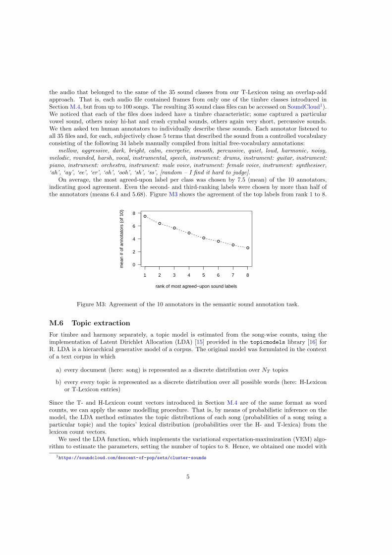
On average, the most agreed-upon label per class was chosen by 7.5 (mean) of the 10 annotators,indicating good agreement. Even the second- and third-ranking labels were chosen by more than half ofthe annotators (means 6.4 and 5.68). Figure M3 shows the agreement of the top labels from rank 1 to 8.

●

●

●

●

●●

●●

1 2 3 4 5 6 7 8

0

2

4

6

8

rank of most agreed−upon sound labels

mea

n #

of a

nnot

ator

s (o

f 10)

Figure M3: Agreement of the 10 annotators in the semantic sound annotation task.

M.6 Topic extraction

For timbre and harmony separately, a topic model is estimated from the song-wise counts, using theimplementation of Latent Dirichlet Allocation (LDA) [15] provided in the topicmodels library [16] forR. LDA is a hierarchical generative model of a corpus. The original model was formulated in the contextof a text corpus in which

a) every document (here: song) is represented as a discrete distribution over NT topics

b) every every topic is represented as a discrete distribution over all possible words (here: H-Lexiconor T-Lexicon entries)

Since the T- and H-Lexicon count vectors introduced in Section M.4 are of the same format as wordcounts, we can apply the same modelling procedure. That is, by means of probabilistic inference on themodel, the LDA method estimates the topic distributions of each song (probabilities of a song using aparticular topic) and the topics’ lexical distribution (probabilities over the H- and T-lexica) from thelexicon count vectors.

We used the LDA function, which implements the variational expectation-maximization (VEM) algo-rithm to estimate the parameters, setting the number of topics to 8. Hence, we obtained one model with

1https://soundcloud.com/descent-of-pop/sets/cluster-sounds

5

8 T-Topics, and one with 8 H-Topics. Topic models allow us to encode every song as a distribution overT- and H-Topics,

qT = (qT1 , qT2 , . . . , q

T8 )

qH = (qH1 , qH2 , . . . , q

H8 )

The probabilities can be interpreted as the proportion of frames in the song belonging to the topic.When it is clear from the context which T- or H-Topic we are concerned with we denote these by theletter q, and their mean over a group of songs by q. Mean values by year for all topics are shown infigure ?? in the main text with 95% confidence intervals based on quantile bootstrapping.

In the same manner, we calculate means and bootstrap confidence intervals for all artists with at least10 chart entries and all Last.fm tags (introduced in Section M.8) with at least 200 occurrences. Theartists with the highest and lowest mean q of each topic and the respective listing of tags can be foundonline.

M.7 Semantic topic annotations

In this section we show how to map the semantic interpretations of our harmony and timbre lexica (seeSection M.5) to the 8 T-Topics and 8 H-Topics. This allows us to work with the topics rather than thelarge number of chord changes and sound classes.

Harmony.

Each H-Topic is defined as a distribution P (EHi ) over all H-lexicon entries EH

i , i = 1, . . . , 193 (the 193different chord changes). The lower half of Table ?? shows the 10 most probable chord changes foreach topic with those that have P (Ei) > 0.01 emphasised in bold. For example, the most likely chordchange in H-Topic 4 is a Major chord followed by another Major chord 7 semitones higher, e.g. C toG. The interpretation of a topic, then, is the coincidence of such chord changes in a piece of music.Interpretations of the 8 H-Topics can be found in Table 1.

Timbre.

In order to obtain interpretations for the T-Topics we map the semantic annotations of the T-lexicon(Section M.5) to the topics. The semantic annotations of the T-lexicon come as a matrix of countsW ∗ = (w∗

ij) of annotation labels j = 1, . . . , 34 for each of the sound classes i = 1, . . . , 35. We firstnormalise the columns w∗

·,j by root-mean-square normalisation to obtain a scaled matrix Wij with theelements

wij =w∗

ij√(1/34)

∑i(w

∗ij)

2. (1)

The matrix W = (wij) expresses the relevance of the jth label for the ith sound class. Since T-Topics arecompositions of sound classes, we can now simply map these relevance values to the topics by multipli-cation. The weight Lj of the jth label for a T-Topic in which sound class ET

i appears with probabilityP (ET

i ) is

Lj =35∑

i=1

wijP (ETi ). (2)

The top 3 labels for each T-Topic can be found in Table 1.

6

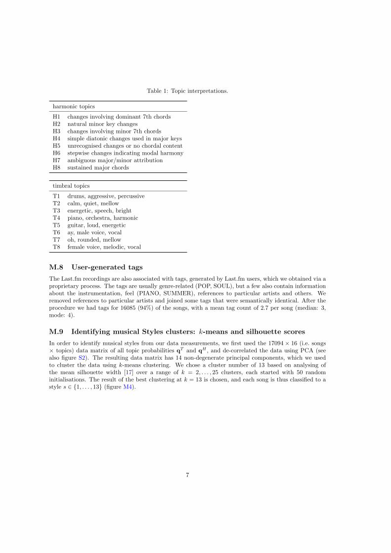
Table 1: Topic interpretations.

harmonic topics

H1 changes involving dominant 7th chordsH2 natural minor key changesH3 changes involving minor 7th chordsH4 simple diatonic changes used in major keysH5 unrecognised changes or no chordal contentH6 stepwise changes indicating modal harmonyH7 ambiguous major/minor attributionH8 sustained major chords

timbral topics

T1 drums, aggressive, percussiveT2 calm, quiet, mellowT3 energetic, speech, brightT4 piano, orchestra, harmonicT5 guitar, loud, energeticT6 ay, male voice, vocalT7 oh, rounded, mellowT8 female voice, melodic, vocal

M.8 User-generated tags

The Last.fm recordings are also associated with tags, generated by Last.fm users, which we obtained via aproprietary process. The tags are usually genre-related (POP, SOUL), but a few also contain informationabout the instrumentation, feel (PIANO, SUMMER), references to particular artists and others. Weremoved references to particular artists and joined some tags that were semantically identical. After theprocedure we had tags for 16085 (94%) of the songs, with a mean tag count of 2.7 per song (median: 3,mode: 4).

M.9 Identifying musical Styles clusters: k-means and silhouette scores

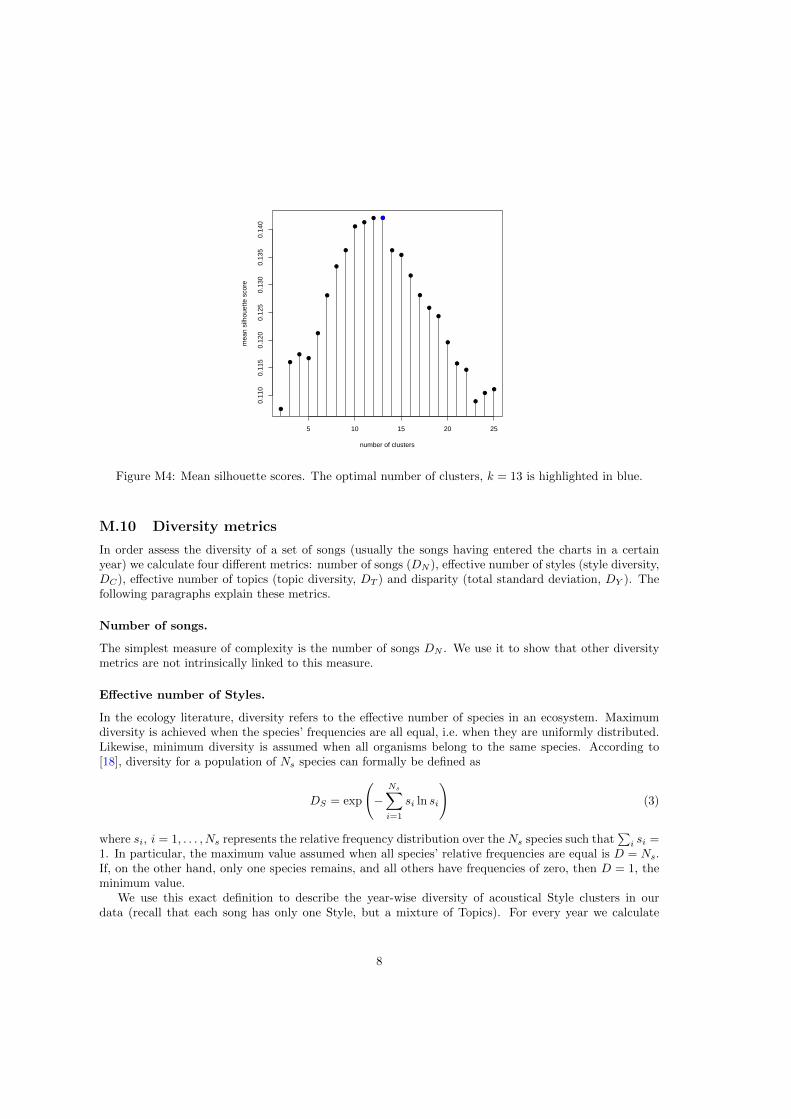
In order to identify musical styles from our data measurements, we first used the 17094 × 16 (i.e. songs× topics) data matrix of all topic probabilities qT and qH , and de-correlated the data using PCA (seealso figure S2). The resulting data matrix has 14 non-degenerate principal components, which we usedto cluster the data using k-means clustering. We chose a cluster number of 13 based on analysing ofthe mean silhouette width [17] over a range of k = 2, . . . , 25 clusters, each started with 50 randominitialisations. The result of the best clustering at k = 13 is chosen, and each song is thus classified to astyle s ∈ {1, . . . , 13} (figure M4).

7

5 10 15 20 25

0.11

00.

115

0.12

00.

125

0.13

00.

135

0.14

0

number of clusters

mea

n si

lhou

ette

sco

re

●

●

●●

●

●

●

●

●●

● ●

●●

●

●

●

●

●

●

●

●

●●

●

Figure M4: Mean silhouette scores. The optimal number of clusters, k = 13 is highlighted in blue.

M.10 Diversity metrics

In order assess the diversity of a set of songs (usually the songs having entered the charts in a certainyear) we calculate four different metrics: number of songs (DN ), effective number of styles (style diversity,DC), effective number of topics (topic diversity, DT ) and disparity (total standard deviation, DY ). Thefollowing paragraphs explain these metrics.

Number of songs.

The simplest measure of complexity is the number of songs DN . We use it to show that other diversitymetrics are not intrinsically linked to this measure.

Effective number of Styles.

In the ecology literature, diversity refers to the effective number of species in an ecosystem. Maximumdiversity is achieved when the species’ frequencies are all equal, i.e. when they are uniformly distributed.Likewise, minimum diversity is assumed when all organisms belong to the same species. According to[18], diversity for a population of Ns species can formally be defined as

DS = exp

(−

Ns∑

i=1

si ln si

)(3)

where si, i = 1, . . . , Ns represents the relative frequency distribution over the Ns species such that∑

i si =1. In particular, the maximum value assumed when all species’ relative frequencies are equal is D = Ns.If, on the other hand, only one species remains, and all others have frequencies of zero, then D = 1, theminimum value.

We use this exact definition to describe the year-wise diversity of acoustical Style clusters in ourdata (recall that each song has only one Style, but a mixture of Topics). For every year we calculate

8

the proportion songs si, i = 1, . . . , 13 belonging to each of the 13 Styles, and hence we use Ns = 13 tocalculate DS ∈ [1, 13].

Effective number of Topics.

The probability q of a certain topic in a song (see Section M.6) provides an estimate of the proportionof frames in a song that belong to that topic. By averaging over the year, we can get an estimate of theproportion q of frames in the whole year, i.e. for all T- and H-Topics we obtain the yearly measurements

qT = (qT1 , qT2 , . . . , q

T8 )

qH = (qH1 , qH2 , . . . , q

H8 ).

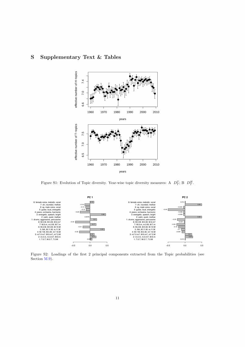
Figuratively, we throw all audio frames of all songs into one big bucket pertaining to a year, and estimatethe proportion of each topic in the bucket. From these yearly estimates of topic frequencies we can nowcalculate the effective number of T- and H-Topics in the same way we calculated the effective number ofStyles (figure S1).

DTT = exp

(−

8∑

i=1

qTi ln qTi

)(4)

DHT = exp

(−

8∑

i=1

qHi ln qHi

)(5)

DT :=DT

T +DHT

2, (6)

where we define DT as the overall measure of topic diversity. DT is shown in the main manuscript (figure4). The individual H- and T-Topic diversities DT

T and DHT are provided in figure ??. It is evident that

the significant diversity decline in the 1980s is mainly due to a decline in timbral topic diversity, whileharmonic diversity shows no sign of sustained decline.

Disparity.

In contrast to diversity, disparity corresponds to morphological variety, variety of measurements. Twoecosystems of equal diversity can have different disparity, depending on the extent to which the phenotypesof species differ. A variety of measures, such as average pairwise character dissimilarity and the totalvariance (sum of univariate variance) [19, 20] have been used to measure disparity. We adopt the squareroot of total variance, a metric called total standard deviation [21, p. 37] as our measure of disparity, i.e.given a set of N observations on T traits as a matrix X = (xn,m), we define it as

DY =

√√√√T∑

t=1

Var(x·,m). (7)

We apply our disparity measure DY to the 14-dimensional matrix of principal components (derivedfrom the topics, as described in Section M.9).

M.11 Identifying musical revolutions

In order to identify points at which the composition of the charts significantly changes, we employ Footenovelty detection [22], a technique often used in MIR [23]. First we pool the 14-dimensional principalcomponent data (see Section M.9) into quarters by their first entry into the charts (January-March, April-June, July-September, October-December) using the quarterly mean of each principal component. We

9

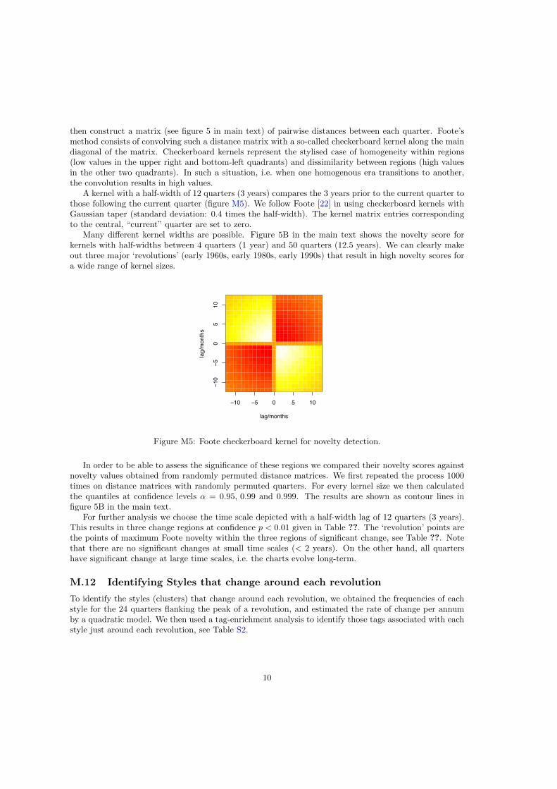
then construct a matrix (see figure 5 in main text) of pairwise distances between each quarter. Foote’smethod consists of convolving such a distance matrix with a so-called checkerboard kernel along the maindiagonal of the matrix. Checkerboard kernels represent the stylised case of homogeneity within regions(low values in the upper right and bottom-left quadrants) and dissimilarity between regions (high valuesin the other two quadrants). In such a situation, i.e. when one homogenous era transitions to another,the convolution results in high values.

A kernel with a half-width of 12 quarters (3 years) compares the 3 years prior to the current quarter tothose following the current quarter (figure M5). We follow Foote [22] in using checkerboard kernels withGaussian taper (standard deviation: 0.4 times the half-width). The kernel matrix entries correspondingto the central, “current” quarter are set to zero.

Many different kernel widths are possible. Figure 5B in the main text shows the novelty score forkernels with half-widths between 4 quarters (1 year) and 50 quarters (12.5 years). We can clearly makeout three major ‘revolutions’ (early 1960s, early 1980s, early 1990s) that result in high novelty scores fora wide range of kernel sizes.

−10 −5 0 5 10

−10

−50

510

lag/months

lag/months

Figure M5: Foote checkerboard kernel for novelty detection.

In order to be able to assess the significance of these regions we compared their novelty scores againstnovelty values obtained from randomly permuted distance matrices. We first repeated the process 1000times on distance matrices with randomly permuted quarters. For every kernel size we then calculatedthe quantiles at confidence levels α = 0.95, 0.99 and 0.999. The results are shown as contour lines infigure 5B in the main text.

For further analysis we choose the time scale depicted with a half-width lag of 12 quarters (3 years).This results in three change regions at confidence p < 0.01 given in Table ??. The ‘revolution’ points arethe points of maximum Foote novelty within the three regions of significant change, see Table ??. Notethat there are no significant changes at small time scales (< 2 years). On the other hand, all quartershave significant change at large time scales, i.e. the charts evolve long-term.

M.12 Identifying Styles that change around each revolution

To identify the styles (clusters) that change around each revolution, we obtained the frequencies of eachstyle for the 24 quarters flanking the peak of a revolution, and estimated the rate of change per annumby a quadratic model. We then used a tag-enrichment analysis to identify those tags associated with eachstyle just around each revolution, see Table S2.

10

S Supplementary Text & Tables

●●●

●●

●●●

●●

●

●

●●

●

●●

●●

●●

●

●●●

●

●

●

●●

●

●●

●

●

●

●

●●●

●●

●●

●●

●

●●

●

1960 1970 1980 1990 2000 2010

6.6

7.0

7.4

years

effe

ctiv

e nu

mbe

r of

H−

topi

cs

●●●

●●

●●●

●●

●

●

●●

●

●●

●●

●●

●

●●●

●

●

●

●●

●

●●

●

●

●

●

●●●

●●

●●

●●

●

●●

●

●

●●●

●●

●●

●●●

●●

●

●●

●●

●

●●

●

●

●

●

●

●●

●●

●●

●

●●

●●

●

●

●

●●●●

●

●

●

●●

●

1960 1970 1980 1990 2000 2010

6.5

7.0

7.5

years

effe

ctiv

e nu

mbe

r of

T−

topi

cs

●

●●●

●●

●●

●●●

●●

●

●●

●●

●

●●

●

●

●

●

●

●●

●●

●●

●

●●

●●

●

●

●

●●●●

●

●

●

●●

●

Figure S1: Evolution of Topic diversity. Year-wise topic diversity measures: A DTT ; B DH

T .

1: 7.0.7, M.0.7, 7.0.M2: m.0.m, m.0.m7, M.9.m

3: m7.0.m7, M.9.m7, m7.3.M4: M.7.M, M.5.M, m7.10.M

5: NA, M.11.M, m.11.M6: M.2.M, M.5.M, M.10.M

7: M.0.m, m.0.M, M.7.m8: M.0.M, M.5.M, M.9.m7

1: drums, aggressive, percussive2: calm, quiet, mellow

3: energetic, speech, bright4: piano, orchestra, harmonic

5: guitar, loud, energetic6: ay, male voice, vocal7: oh, rounded, mellow

8: female voice, melodic, vocal

PC 1

−0.5 0.0 0.5

0.0580.17

0.12−0.32

0.43−0.21

0.17−0.43

0.20.0078

0.46−0.29

−0.12−0.14−0.16

0.12

1: 7.0.7, M.0.7, 7.0.M2: m.0.m, m.0.m7, M.9.m

3: m7.0.m7, M.9.m7, m7.3.M4: M.7.M, M.5.M, m7.10.M

5: NA, M.11.M, m.11.M6: M.2.M, M.5.M, M.10.M

7: M.0.m, m.0.M, M.7.m8: M.0.M, M.5.M, M.9.m7

1: drums, aggressive, percussive2: calm, quiet, mellow

3: energetic, speech, bright4: piano, orchestra, harmonic

5: guitar, loud, energetic6: ay, male voice, vocal7: oh, rounded, mellow

8: female voice, melodic, vocal

PC 2

−0.5 0.0 0.5

0.0130.240.2

−0.091−0.1

−0.19−0.24

−0.021−0.22

0.49−0.039−0.038

−0.49−0.043

0.490.014

1: X7.0.7, M.0.7, X7.0.M2: m.0.m, m.0.m7, M.9.m

3: m7.0.m7, M.9.m7, m7.3.M4: M.7.M, M.5.M, m7.10.M

5: NA, M.11.M, m.11.M6: M.2.M, M.5.M, M.10.M

7: M.0.m, m.0.M, M.7.m8: M.0.M, M.5.M, M.9.m7

1: drums, aggressive, percussive2: calm, quiet, mellow

3: energetic, speech, bright4: piano, orchestra, harmonic

5: guitar, loud, energetic6: ay, male voice, vocal7: oh, rounded, mellow

8: female voice, melodic, vocal

PC 3

−0.5 0.0 0.5

−0.09−0.36

−0.450.27

0.40.073

−0.120.3

−0.190.13

0.36−0.3

−0.160.120.11

0.031

1: X7.0.7, M.0.7, X7.0.M2: m.0.m, m.0.m7, M.9.m

3: m7.0.m7, M.9.m7, m7.3.M4: M.7.M, M.5.M, m7.10.M

5: NA, M.11.M, m.11.M6: M.2.M, M.5.M, M.10.M

7: M.0.m, m.0.M, M.7.m8: M.0.M, M.5.M, M.9.m7

1: drums, aggressive, percussive2: calm, quiet, mellow

3: energetic, speech, bright4: piano, orchestra, harmonic

5: guitar, loud, energetic6: ay, male voice, vocal7: oh, rounded, mellow

8: female voice, melodic, vocal

PC 4

−0.5 0.0 0.5

0.610.056

−0.42−0.32

−0.01−0.18

0.320.037

−0.22−0.12−0.045

0.19−0.1

0.290.11

−0.016

1: X7.0.7, M.0.7, X7.0.M2: m.0.m, m.0.m7, M.9.m

3: m7.0.m7, M.9.m7, m7.3.M4: M.7.M, M.5.M, m7.10.M

5: NA, M.11.M, m.11.M6: M.2.M, M.5.M, M.10.M

7: M.0.m, m.0.M, M.7.m8: M.0.M, M.5.M, M.9.m7

1: drums, aggressive, percussive2: calm, quiet, mellow

3: energetic, speech, bright4: piano, orchestra, harmonic

5: guitar, loud, energetic6: ay, male voice, vocal7: oh, rounded, mellow

8: female voice, melodic, vocal

PC 5

−0.5 0.0 0.5

−0.20.34

−0.016−0.0081

−0.092−0.039

−0.140.035

−0.5−0.22

0.096−0.026

0.120.13

−0.140.67

1: X7.0.7, M.0.7, X7.0.M2: m.0.m, m.0.m7, M.9.m

3: m7.0.m7, M.9.m7, m7.3.M4: M.7.M, M.5.M, m7.10.M

5: NA, M.11.M, m.11.M6: M.2.M, M.5.M, M.10.M

7: M.0.m, m.0.M, M.7.m8: M.0.M, M.5.M, M.9.m7

1: drums, aggressive, percussive2: calm, quiet, mellow

3: energetic, speech, bright4: piano, orchestra, harmonic

5: guitar, loud, energetic6: ay, male voice, vocal7: oh, rounded, mellow

8: female voice, melodic, vocal

PC 6

−0.5 0.0 0.5

0.190.0033

−0.23−0.06

−0.20.063

0.250.11

−0.0270.34

−0.16−0.39

0.32−0.57

0.0480.23

1: X7.0.7, M.0.7, X7.0.M2: m.0.m, m.0.m7, M.9.m

3: m7.0.m7, M.9.m7, m7.3.M4: M.7.M, M.5.M, m7.10.M

5: NA, M.11.M, m.11.M6: M.2.M, M.5.M, M.10.M

7: M.0.m, m.0.M, M.7.m8: M.0.M, M.5.M, M.9.m7

1: drums, aggressive, percussive2: calm, quiet, mellow

3: energetic, speech, bright4: piano, orchestra, harmonic

5: guitar, loud, energetic6: ay, male voice, vocal7: oh, rounded, mellow

8: female voice, melodic, vocal

PC 7

−0.5 0.0 0.5

−0.510.54

−0.38−0.15

−0.00870.23

0.30.056

0.0430.0240.029

−0.016−0.0032

0.0630.12

−0.32

1: X7.0.7, M.0.7, X7.0.M2: m.0.m, m.0.m7, M.9.m

3: m7.0.m7, M.9.m7, m7.3.M4: M.7.M, M.5.M, m7.10.M

5: NA, M.11.M, m.11.M6: M.2.M, M.5.M, M.10.M

7: M.0.m, m.0.M, M.7.m8: M.0.M, M.5.M, M.9.m7

1: drums, aggressive, percussive2: calm, quiet, mellow

3: energetic, speech, bright4: piano, orchestra, harmonic

5: guitar, loud, energetic6: ay, male voice, vocal7: oh, rounded, mellow

8: female voice, melodic, vocal

PC 8

−0.5 0.0 0.5

0.0530.11

−0.24−0.056

0.230.049

−0.310.079

0.049−0.19

0.110.55

−0.088−0.62

0.0740.054

Figure S2: Loadings of the first 2 principal components extracted from the Topic probabilities (seeSection M.9).

11

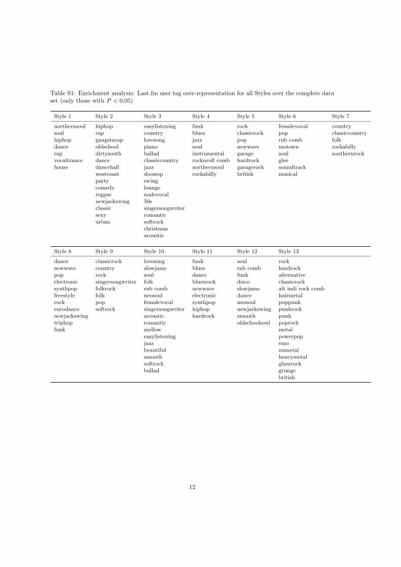
Table S1: Enrichment analysis: Last.fm user tag over-representation for all Styles over the complete dataset (only those with P < 0.05)

Style 1 Style 2 Style 3 Style 4 Style 5 Style 6 Style 7

northernsoul hiphop easylistening funk rock femalevocal countrysoul rap country blues classicrock pop classiccountryhiphop gangstarap lovesong jazz pop rnb comb folkdance oldschool piano soul newwave motown rockabillyrap dirtysouth ballad instrumental garage soul southernrockvocaltrance dance classiccountry rocknroll comb hardrock gleehouse dancehall jazz northernsoul garagerock soundtrack

westcoast doowop rockabilly british musicalparty swingcomedy loungereggae malevocalnewjackswing 50sclassic singersongwritersexy romanticurban softrock

christmasacoustic

Style 8 Style 9 Style 10 Style 11 Style 12 Style 13

dance classicrock lovesong funk soul rocknewwave country slowjams blues rnb comb hardrockpop rock soul dance funk alternativeelectronic singersongwriter folk bluesrock disco classicrocksynthpop folkrock rnb comb newwave slowjams alt indi rock combfreestyle folk neosoul electronic dance hairmetalrock pop femalevocal synthpop neosoul poppunkeurodance softrock singersongwriter hiphop newjackswing punkrocknewjackswing acoustic hardrock smooth punktriphop romantic oldschoolsoul poprockfunk mellow metal

easylistening powerpopjazz emobeautiful numetalsmooth heavymetalsoftrock glamrockballad grunge

british

12

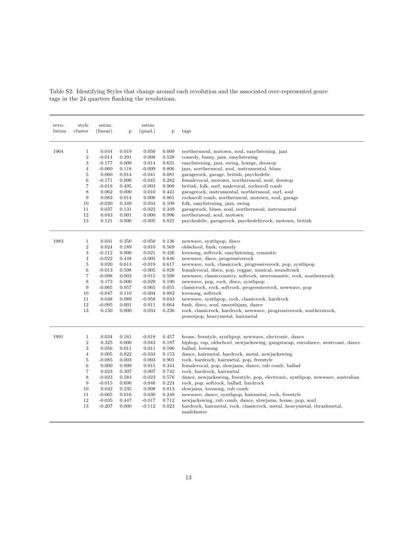
Table S2: Identifying Styles that change around each revolution and the associated over-represented genretags in the 24 quarters flanking the revolutions.

revo- style estim. estim.lution cluster (linear) p (quad.) p tags

1964 1 0.044 0.019 0.050 0.009 northernsoul, motown, soul, easylistening, jazz2 -0.014 0.291 0.008 0.528 comedy, funny, jazz, easylistening3 -0.177 0.000 0.014 0.631 easylistening, jazz, swing, lounge, doowop4 -0.060 0.118 -0.009 0.806 jazz, northernsoul, soul, instrumental, blues5 0.060 0.014 -0.041 0.081 garagerock, garage, british, psychedelic6 -0.171 0.000 -0.045 0.282 femalevocal, motown, northernsoul, soul, doowop7 -0.018 0.495 -0.003 0.908 british, folk, surf, malevocal, rocknroll comb8 0.062 0.000 0.010 0.441 garagerock, instrumental, northernsoul, surf, soul9 0.083 0.014 0.006 0.861 rocknroll comb, northernsoul, motown, soul, garage

10 -0.020 0.349 0.034 0.109 folk, easylistening, jazz, swing11 0.037 0.131 -0.022 0.349 garagerock, blues, soul, northernsoul, instrumental12 0.043 0.001 0.000 0.996 northernsoul, soul, motown13 0.121 0.000 -0.005 0.821 psychedelic, garagerock, psychedelicrock, motown, british

1983 1 0.031 0.350 -0.050 0.136 newwave, synthpop, disco2 0.024 0.189 0.010 0.569 oldschool, funk, comedy3 -0.112 0.000 0.021 0.426 lovesong, softrock, easylistening, romantic4 -0.022 0.448 -0.005 0.846 newwave, disco, progressiverock5 0.020 0.614 -0.019 0.617 newwave, rock, classicrock, progressiverock, pop, synthpop6 -0.013 0.598 -0.005 0.828 femalevocal, disco, pop, reggae, musical, soundtrack7 -0.098 0.003 0.015 0.598 newwave, classiccountry, softrock, newromantic, rock, southernrock8 0.173 0.000 -0.029 0.190 newwave, pop, rock, disco, synthpop9 -0.065 0.057 0.065 0.055 classicrock, rock, softrock, progressiverock, newwave, pop

10 -0.047 0.110 -0.004 0.882 lovesong, softrock11 0.048 0.089 -0.058 0.043 newwave, synthpop, rock, classicrock, hardrock12 -0.095 0.001 0.011 0.664 funk, disco, soul, smoothjazz, dance13 0.150 0.000 0.034 0.236 rock, classicrock, hardrock, newwave, progressiverock, southernrock,

powerpop, heavymetal, hairmetal

1991 1 0.034 0.161 -0.018 0.457 house, freestyle, synthpop, newwave, electronic, dance2 0.325 0.000 0.043 0.187 hiphop, rap, oldschool, newjackswing, gangstarap, eurodance, westcoast, dance3 0.056 0.011 0.011 0.596 ballad, lovesong4 0.005 0.822 -0.034 0.153 dance, hairmetal, hardrock, metal, newjackswing5 -0.085 0.003 0.003 0.901 rock, hardrock, hairmetal, pop, freestyle6 0.000 0.999 0.015 0.344 femalevocal, pop, slowjams, dance, rnb comb, ballad7 0.023 0.307 0.007 0.742 rock, hardrock, hairmetal8 -0.023 0.584 -0.023 0.576 dance, newjackswing, freestyle, pop, electronic, synthpop, newwave, australian9 -0.015 0.690 0.046 0.224 rock, pop, softrock, ballad, hardrock

10 0.042 0.235 0.008 0.813 slowjams, lovesong, rnb comb11 -0.065 0.016 0.030 0.248 newwave, dance, synthpop, hairmetal, rock, freestyle12 -0.035 0.447 -0.017 0.712 newjackswing, rnb comb, dance, slowjams, house, pop, soul13 -0.207 0.000 -0.112 0.023 hardrock, hairmetal, rock, classicrock, metal, heavymetal, thrashmetal,

madchester

13

References

[1] Mauch M, Ewert S. The Audio Degradation Toolbox and its Application to Robustness Evaluation.In: Proceedings of the 14th International Society of Music Information Retrieval Conference (ISMIR2013); 2013. p. 83–88.

[2] Fujishima T. Real Time Chord Recognition of Musical Sound: a System using Common Lisp Music.In: Proceedings of the International Computer Music Conference (ICMC 1999); 1999. p. 464–467.

[3] Mauch M, Dixon S. Simultaneous Estimation of Chords and Musical Context from Audio. IEEETransactions on Audio, Speech, and Language Processing. 2010;18(6):1280–1289.

[4] Bartsch MA, Wakefield GH. Audio thumbnailing of popular music using chroma-based representa-tions. IEEE Transactions on Multimedia. 2005;7(1):96–104.

[5] Muller M, Kurth F. Towards structural analysis of audio recordings in the presence of musicalvariations. EURASIP Journal on Applied Signal Processing. 2007;2007(1):163–163.

[6] Mauch M, Dixon S. Approximate note transcription for the improved identification of difficult chords.Proceedings of the 11th International Society for Music Information Retrieval Conference (ISMIR2010). 2010;p. 135–140.

[7] Davis S, Mermelstein P. Comparison of parametric representations for monosyllabic word recognitionin continuously spoken sentences. IEEE Transactions on Acoustics, Speech and Signal Processing.1980;28(4):357–366.

[8] Foote JT. Content-Based Retrieval of Music and Audio. Proceedings of SPIE. 1997;138:138–147.

[9] Ito M, Donaldson RW. Zero-crossing measurements for analysis and recognition of speech sounds.IEEE Transactions on Audio and Electroacoustics. 1971;19(3):235–242.

[10] Gouyon F, Pachet F, Delerue O. On the use of zero-crossing rate for an application of classification ofpercussive sounds. In: Proceedings of the COST G-6 Conference on Digital Audio Effects (DAFX-00);2000. p. 1–6.

[11] McLachlan GJ, Peel D. Finite Mixture Models. Hoboken, NJ: John Wiley & Sons; 2000.

[12] Burgoyne JA, Wild J, Fujinaga I. An expert ground-truth set for audio chord recognition andmusic analysis. In: Proceedings of the 12th International Conference on Music Information Retrieval(ISMIR 2011); 2011. p. 633–638.

[13] Papadopoulos H, Peeters G. Large-scale Study of Chord Estimation Algorithms Based on ChromaRepresentation and HMM. In: International Workshop on Content-Based Multimedia Indexing;2007. p. 53–60.

[14] Mauch M, Dixon S, Harte C, Fields B, Casey M. Discovering chord idioms through Beatles and RealBook songs. In: Proceedings of the 8th International Conference on Music Information Retrieval(ISMIR 2007); 2007. p. 255–258.

[15] Blei DM, Ng AY, Jordan MI. Latent dirichlet allocation. Journal of Machine Learning Research.2003;3:993–1022.

[16] Hornik K, Grun B. topicmodels: An R package for fitting topic models. Journal of StatisticalSoftware. 2011;40(13):1–30.

[17] Rousseeuw PJ. Silhouettes: a graphical aid to the interpretation and validation of cluster analysis.Journal of computational and applied mathematics. 1987;20:53–65.

14

[18] Jost L. Entropy and diversity. Oikos. 2006;113(2):363–375.

[19] Erwin DH. DISPARITY: MORPHOLOGICAL PATTERN AND DEVELOPMENTAL CONTEXT.Palaeontology. 2007;50(1):57–73.

[20] Foote M. The evolution of morphological diversity. Annual Review of Ecology and Systematics.1997;.

[21] Hallgrımsson B, Hall BK. Variation: A Central Concept in Biology. Academic Press; 2011.

[22] Foote J. Automatic audio segmentation using a measure of audio novelty. In: IEEE InternationalConference on Multimedia and Expo. vol. 1; 2000. p. 452–455.

[23] Smith JBL, Chew E. A Meta-Analysis of the MIREX Structure Segmentation Task. In: Proceedingsof the 14th International Society for Music Information Retrieval Conference; 2013. .

15