the emergence of range limits in advective · the emergence of range limits in advective...

THE EMERGENCE OF RANGE LIMITS IN ADVECTIVE

ENVIRONMENTS

KING-YEUNG LAM1, YUAN LOU1,2, AND FRITHJOF LUTSCHER3

Abstract. In this paper, we study the asymptotic profile of the steady state of a reaction-diffusion-advection model in ecology proposed in [13, 17]. The model describes the populationdynamics of a single species experiencing a uni-directional flow. We show the existence ofone or more internal transition layers and determine their locations. Such locations can beunderstood as the upstream invasion limits of the species. It turns out that these invasionlimits are connected to the upstream spreading speed of the species and is sometimes subjectto the effect of migration from upstream source patches.

1. Introduction

Most species have spatially limited distributions [1]. Ecologists have identified a few basicaspects of dispersal and birth-death dynamics that can explain several mechanisms underlyingrange limits [7]. For example, local biotic and abiotic conditions determine the basic rate ofincrease of a population. The species is expected to be present where its rate of increase ispositive (its “niche”) and absent where this rate is negative. A range limit then indicates asign change of this rate of increase. Dispersal can enlarge a species’ range and maintain apopulation in regions where the intrinsic growth rate is negative (source-sink dynamics). Instreams and rivers, water flow can induce a strong directional bias in dispersal. What then isthe effect of this biased dispersal on the emergence of range limits?

Abiotic conditions can change considerably along the course of a river or stream. Tem-perature and nutrient loading tend to increase downstream whereas shading decreases [18].But conditions need not change monotonically. Local habitat attributes are also affectedby substrate, confluences, dams, or point source disturbances such as waste-water treatmentplants. Accordingly, algal community composition varies considerably between upstream anddownstream [16, 21] and with it the food chain that it can support. These assemblages areformed by the combined effects of local growth conditions (source and sinks) and of passivetransport in the water column. Because of the strong bias of transport, one could expect aspecies to be absent from the upstream end of its niche or source region and persist in sinkhabitats further downstream. Can one quantify this effect of hydrology on the actual rangeof a species?

1Department of Mathematics, Ohio State University, Columbus, OH 432102Institute for Mathematical Sciences, Renmin University of China, Beijing, 100872, PRC3Department of Mathematics and Statistics, and Department of Biology, University of Ot-

tawa, Ottawa, ON, K1N6N5, CanadaE-mail addresses: [email protected], [email protected], [email protected]: November 28, 2015.KYL and YL are partially supported by the NSF grant DMS–1411476. YL is also partially supported by

the Fundamental Research Funds for the Central Universities, and the Research Funds of Renmin Universityof China. FL is partially funded by an Individual Discovery Grant from NSERC.

Key words: reaction-diffusion, advection, range limit, transition layer, dispersal.AMS subject classification: 35K57, 92D15, 92D25.

1

2 RANGE LIMITS IN ADVECTIVE ENVIRONMENTS

The dynamics of a spatially distributed species, moving passively in a stream or river, havebeen modeled with a reaction-advection-diffusion equation to explore population persistenceand the so-called “drift paradox” [13, 17]. In the simplest case, the equation for the densityu(x, t) of a population at time t and location x is given by

(1) ut = Duxx − qux + u(r − κu),

where D > 0 is the diffusion coefficient, q > 0 is the flow speed in the direction of increasingx, r is the population growth rate at low density, and κ denotes the strength of intra-specificcompetition. (Subscripts denote partial derivatives.) Lutscher and coauthors studied thismodel (and a two-species extension) with linearly increasing growth function r = r(x) (i.e.the habitat quality of downstream location is better than the upstream location) and observedthe emergence of upstream range limits [11]. Specifically, when the stream was long, the steadystate population showed a sharp transition layer from low to high density, much steeper thanthe local growth conditions would predict. Numerically, the authors found that a speciesinitially occupying a downstream region may propagate upstream in a wave-like fashion withdecreasing speed. This upstream invasion wave comes to a halt at some location x, eventhough local growth conditions are favorable upstream of that location, i.e. r(x) > 0 forx < x.

Traveling waves are well studied for the Fisher model, given by equation (1) with q = 0 and

constant r. They arise at a minimal speed c∗ = 2√rD, the asymptotic spreading speed [20].

In an environment with unidirectional flow of speed q > 0, there are two spreading speeds, onein the direction of the flow (downstream), given by c∗+q, and one against the flow (upstream),given by c∗−q [13]. When the flow speed is lower than c∗, then the upstream spreading speedis positive and the population can spread against the flow. When the flow speed is higherthan c∗, then the upstream speed is negative and the population retreats downstream.

When growth conditions vary spatially, r = r(x) is a non-constant function. It is then

tempting to define the “local upstream spreading speed” as 2√r(x)D − q [7]. A range limit

then emerges where the local upstream spreading speed is zero. For a monotone growth

function r(x), there is a unique location x∗ defined by r(x∗) = q2

4D . Numerical simulations formodel (1) indicated that, indeed, x = x∗ [11].

To see why the steady state density u can be very small even though the local growth rater(x) is positive, we introduce the transformation u(x, t) = w(x, t)eqx/(2D). Then w satisfiesthe equation

(2) wt = Dwxx + w

(r(x)− q2

4D− weqx/(2D)

),

with local intrinsic growth rate r(x)− q2

4D . Hence, the stream flow can be viewed as decreasing

the local growth rate. Specifically, regions with r(x) > q2

4D are population dynamic sources

whereas regions with r(x) < q2

4D are sinks.The first purpose of this paper is to prove the existence of a steady state profile with the

steep transition layer as observed in numerical simulations [11] when the growth functionis monotone increasing and the stream segment is long. In the second part of the paper,

we consider the case that the adjusted growth function r(x) − q2

4D changes sign more thanonce. In this case, we could expect multiple transition layers of u occurring at locations x∗iwith r(x∗i ) −

q2

4D = 0. We show that there is at most one transition layer per source patch,i.e. an interval where r > 0. More specifically, when there is only one source patch and thepopulation persists, then there is only one transition layer, even if the adjusted growth rate is

RANGE LIMITS IN ADVECTIVE ENVIRONMENTS 3

negative somewhere. If there are two or more disjoint source patches, then a second transitionlayer maybe located further upstream than would be predicted by the locations x∗i . Thisphenomenon arises when emigrants from high-density regions upstream contribute to localpopulation growth at the next downstream source patch. We give a precise characterizationof the location of a second transition layer.

We introduce the model with boundary conditions and scalings in detail in Section 2.We state all the main results in Section 3, and present numerical illustrations in Section 4.Auxiliary lemmas are given in Section 5. Proofs of the main theorems are presented in Section6. Finally, an extension of our results concerning a boundary transition layer is discussed inSection 7.

2. Model description

We denote the density of the species at time t and location x in the bounded interval [0, L]with u(x, t), where L is the length of the river. We denote the diffusion constant by D > 0and the flow speed by q > 0 so that advection points to increasing x-values. We supplementthe equation in model (1) with generalized Danckwerts boundary condition at the upstream(x = 0) and downstream (x = L) end. The model then reads

(3)

{ut = Duxx − qux + u(r(x)− κu) for 0 < x < L, t > 0,Dux(0)− qu(0) = qbuu(0), Dux(L)− qu(L) = −qbdu(L) for t > 0.

The (dimensionless) parameters bu and bd determine the magnitude of population loss at theupstream and downstream boundaries, respectively. No-flux condition at the downstreamboundary corresponds to bd = 0, whereas hostile condition results as bd →∞. An importantintermediate case is bd = 1, when net-movement across the boundary results only from dif-fusion. For a more detailed discussion and derivation from a random walk model, we referto [8, 10]. The function r(x) stands for the quality of the habitat; the population can growwhere r > 0 and will decline where r < 0.

Based on the numerical results in [11], we consider the case where the river is very longcompared to the scales of advective and diffusive movement. We introduce non-dimensionalvariables t = t/τ, x = x/L and u = κu, and a small parameter ε = qτ/L. Since we will studythe steady-sate problem, we may choose the time scale τ = 1. With this scaling, the modelbecomes

(4)

{ut = ε2Duxx − εux + u(r − u) for 0 < x < 1, t > 0,

εDux(0, t)− u(0, t) = buu(0, t), εDux(1, t)− u(1, t) = −bdu(1, t), for t > 0,

where D = D/q2 is the rescaled diffusion coefficient and r(x) = r(x) denotes the rescaledgrowth profile on [0, 1]. After dropping “ˆ” for ease of notation, we finally obtain our dimen-sionless model system as

(5)

{ut = ε2Duxx − εux + u(r − u) for 0 < x < 1, t > 0,εDux(0, t)− u(0, t) = buu(0, t), εDux(1, t)− u(1, t) = −bdu(1, t), for t > 0.

The dynamics of this model are completely determined by the linear stability of the trivialsolution since the system is monotone [4]. If the zero solution is locally asymptotically stable,then it is globally stable. If it is unstable, then there is a unique positive steady state, whichis globally stable among non-negative, non-trivial solutions. The non-trivial steady-statesolution u(x) of (5) satisfies the equation

(6)

{ε2Duxx − εux + u(r − u) = 0 for 0 < x < 1,εDux(0)− u(0) = buu(0), εDux(1)− u(1) = −bdu(1).


In this paper, we study existence conditions for u and its spatial profile.

3. Main Results

In this section, we explain and interpret our main results about the existence and spatialprofile of the positive solution u(x) of (6). We formulate all of our results in terms of the localupstream spreading speed, which, in the parametrization of (5) is given by

c(x) =

{ε(2√r(x)D − 1) when r(x) ≥ 0,

−ε when r(x) < 0.

Note that when r < 0, then c is simply the transformed flow speed −ε.

3.1. Persistence Results. It is well-known that the persistence of the single species governedby diffusive-logistic equation (5) is characterized by the principal eigenvalue λ1 of{

ε2Dφxx − εφx + rφ+ λ1φ = 0 for 0 < x < 1,εDφx(0)− φ(0) = buφ(0), εDφx(1)− φ(1) = −bdφ(1).

Namely, if λ1 < 0 then there exists a unique positive steady state of (5) which is also globallyasymptotically stable among all non-negative, non-trivial solutions; and if λ1 ≥ 0, then thezero solution is globally asymptotically stable. See, e.g. [4, P. 150] and also [3, 6, 12, 15]. Theprincipal eigenvalue λ1 is in general a nonlinear function of coefficients ε,D, r(x), bu, bd.

We state below two practical persistence/extinction results that are uniform for all (small)values of ε which are relevant to our investigation.

Theorem 3.1. If max[0,1] c > 0, i.e. max[0,1] r >14D , then there exists ε0 > 0 such that for

all ε ∈ (0, ε0) (and all bu, bd ≥ 0), equation (6) has a unique positive solution u that is theglobally asymptotically stable steady state for equation (5), among all non-negative and notidentically zero initial data.

Theorem 3.2. If max[0,1] c ≤ 0, i.e. max[0,1] r ≤ 14D , and if bd ≥ 1

2 , then for all ε > 0, equation(6) has no positive solution, and the zero solution of equation (5) is globally asymptoticallystable among all non-negative and not identically zero initial data.

Theorem 3.1 states that when the upstream spreading speed is positive somewhere, then alocally introduced population can spread in both directions and persist in the habitat. Thisresult holds only when the habitat is sufficiently long so that potential boundary loss doesnot impact population survival. Specifically, we are not considering a minimal domain-sizeproblem here.

As a complement to Theorem 3.1, Theorem 3.2 shows that the population cannot persistin any upstream portion of the river if its upstream invasion speed is non-positive. Thisresult arises only when there is some population loss at the downstream end of the habitat.For example, if both boundary conditions are no-flux conditions (i.e. bu = bd = 0), then thepopulation will persist as long as some appropriate average of the growth rate is positive,

i.e.∫ 10 r(x) exp(x/(εD))dx > 0.

We refer the interested reader to previous work on population persistence [8, 17, 19]. Wenote that if no-flux boundary conditions are imposed at both ends (i.e. bu = bd = 0), and ifr(x) > 0, then the population always persists, regardless of ε,D. In particular, the conditionthat bd ≥ 1

2 is indispensable. A recent detailed study of the influence of upstream anddownstream loss rates is given in [9].

In the rest of this section, we will focus on the Danckwerts boundary condition, whichcorresponds to no-flux upstream conditions (bu = 0) and Neumann downstream conditions


(bd = 1). We note also that Neumann conditions only describe a no-flux scenario when thereis no advection (q = 0).

3.2. Single Internal Transition Layer. We define the upstream invasion limit as the fur-thest upstream location where the upstream invasion speed is positive, i.e.

(7) z1 = inf{x ∈ (0, 1) : c(x) > 0} = inf{x ∈ (0, 1) : r(x) > 1/4D}.We note that when max[0,1] c > 0, i.e. max[0,1] r >

14D , then z1 is well defined and z1 ∈ [0, 1].

In addition, z1 is uniquely defined even when r(x) is constant in some intervals.The following result shows that, in the case of z1 > 0, how the range of species can be

characterized by the upstream invasion limit:

Theorem 3.3. Suppose that max[0,1] c > 0, z1 ∈ (0, 1) and that r(x) > 0 for x > z1. Then,as ε→ 0,

u→ r(x)1[z1,1] locally uniformly in [0, 1] \ {z1},where 1[z1,1] denotes the characteristic function of the interval [z1, 1].

The statement of Theorem 3.3 is illustrated in Figure 1. See also Figure 2 for a numericalexample. When the upstream invasion limit z1 is below the upstream end of the habitat, then,in a long river, the population will approach a spatial profile with a single internal transitionlayer from near zero density upstream of z1 to carrying capacity downstream of z1.

3.3. Multiple Internal Transition Layers. Theorem 3.3 requires r > 0 downstream ofz1 = inf{x ∈ [0, 1] : r(x) > 1/(4D)}. When r < 0 for some intermediate region downstreamof z1 and r(1) > 1/(4D), then there will be a second internal transition layer. The mainquestion is the location of this second layer. To this end, we study a representative situation.

Suppose that there exists a partition 0 < x1 < x2 < x3 < 1, such that

(8) r(x) < 0 in [0, x1) ∪ (x2, x3) and r(x) > 0 in (x1, x2) ∪ (x3, 1].

Naively, we would expect another internal transition layer located at the second invasion limitz2, given by

(9) z2 := inf{x ∈ (x3, 1) : r(x) > 1/4D}.Our next theorem shows that while this situation can occur, more subtle effects may arise.In fact, the second transition layer may be located upstream of z2; see Figure 3.

Specifically, we require the maximum upstream invasion speed to be positive in both patches[x1, x2] and [x3, 1], i.e.

max[x1,x2]

c(x) > 0 and max[x3,1]

c(x) > 0,

or equivalently,

(10) max[x1,x2]

r(x) > 14D and max

[x3,1]r(x) > 1

4D .

When c(x) < 0 (i.e. r(x) < 1/(4D)), we can define the quantities

(11) α±(x) :=1±√

1−4Dr(x)2D .

Note that α+ is always positive whereas α− has the same sign as r(x).It turns out that the sign of

∫ z2x2α−(t) dt plays a critical role in determining the location of

the second internal transition layer.

Theorem 3.4. Suppose r(x) satisfies conditions (8) and (10).


(a) Assume that∫ z2x2α−(t) dt ≤ 0. Then as ε→ 0,

u→ r(x)[1[z1,x2] + 1[z2,1]

]locally uniformly in [0, 1] \ {z1, z2},

where z1 and z2 are defined in (7) and (9), respectively.(b) Assume that

∫ z2x2α−(t) dt > 0. Then as ε→ 0,

u→ r(x)[1[z1,x2] + 1[z2,1]

]locally uniformly in [0, 1] \ {z1, z2},

where z2 ∈ (x3, z2) is uniquely determined by the relation

∫ z2

x2

α−(t) dt = 0.

The statement of this theorem is illustrated in Figures 1 and 3. The first transition layer islocated at the upstream invasion limit z1 as before. Downstream of the region where r < 0,there is a second point, z2, where the upstream invasion speed is zero. If we only consider theregion downstream of r < 0, then we would expect a transition layer at z2 based on the samereasoning as the layer at z1. This reasoning is correct when the region r < 0 is large. However,if this region is small, then there will be immigration of individuals from the upstream patch[z1, x2] to the downstream patch. This influx of individuals allows the population to establishfurther upstream of z2, more specifically, at z2.

Figure 1. Left panel: Illustration of Theorem 3.3. Right panel: Illustrationof Theorem 3.4.

4. Numerical Results

In this section, we present some numerical results that complement and illustrate ouranalytical results from the previous section. We begin with the shape and location of a singletransition layer in the case of a monotone, increasing resource function as in Theorem 3.3.

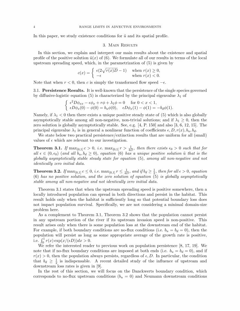
We choose the simple linear function r(x) = x to represent how habitat quality is increasingdownstream, and we fix a diffusion coefficient of D = 1/2. The condition r(z1) = 1/(4D) givesa theoretical upstream invasion limit of z1 = 1/2. We illustrate the statement of Theorem 3.3in Figure 2. We plot the resource function, r(x), and the steady state solution, u(x), for thethree different values of ε. As ε decreases, the steady state profile becomes steeper and thetransition layer “moves closer” to the theoretical value z1. We evaluated the latter distanceby numerically calculating the value y1 such that u(y1) = r(z1)/2 = 1/2. The results aresummarized in Table 1.


ε 0.02 0.01 0.005y1 − z1 0.139 0.0775 0.022

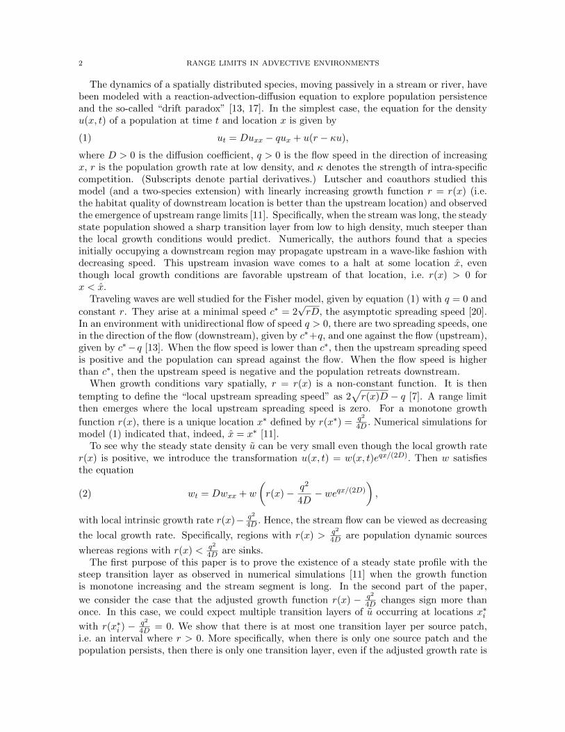
Table 1. Distance between the transition layer and the upstream invasionlimit for linearly increasing r(x). We conjecture that y1 − z1 is of the order ofε, i.e. the actual location of the transition layer lies in an ε-neighborhood ofz1.

Figure 2. Monotone increasing resource function r(x) and steady-state profileu(x) for three values of ε = 0.02 (dash-dot), ε = 0.01 (dashed), and ε = 0.005(solid).

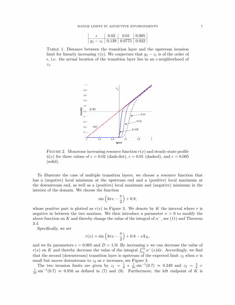
To illustrate the case of multiple transition layers, we choose a resource function thathas a (negative) local minimum at the upstream end and a (positive) local maximum atthe downstream end, as well as a (positive) local maximum and (negative) minimum in theinterior of the domain. We choose the function

sin(

3πx− π

2

)+ 0.8,

whose positive part is plotted as r(x) in Figure 3. We denote by K the interval where r isnegative in between the two maxima. We then introduce a parameter ν > 0 to modify theabove function on K and thereby change the value of the integral of α−, see (11) and Theorem3.4.

Specifically, we set

r(x) = sin(

3πx− π

2

)+ 0.8− ν1K ,

and we fix parameters ε = 0.005 and D = 1/6. By increasing ν we can decrease the value ofr(x) on K and thereby decrease the value of the integral

∫ z2x2α−(x)dx. Accordingly, we find

that the second (downstream) transition layer is upstream of the expected limit z2 when ν issmall but moves downstream to z2 as ν increases, see Figure 3.

The two invasion limits are given by z1 = 16 + 1

3π sin−1(0.7) ≈ 0.249 and z2 = 56 +

13π sin−1(0.7) ≈ 0.916 as defined in (7) and (9). Furthermore, the left endpoint of K is


Figure 3. An oscillating resource function, r(x), (dashed) and the steady-state profile u(x) for various values of ν = 0, 0.5, 1, 2. Increasing ν changesr(x) in the region where r < 0 between the two maxima. Fixed parametersare ε = 0.005 and D = 1/6.

x2 = 12 + 1

3π sin−1(0.8) ≈ 0.598. The values of the integral∫ z2

x2

α−(x)dx =

∫ z2

x2

1−√

1− 4Dr(x)

2Ddx.

are listed in Table 2.

ν 0 0.5 1 2 5∫ z2x2α−(x)dx 0.1613 0.1003 0.046 -0.0488 -0.2726

y1 − z1 -0.017 -0.017 -0.017 -0.017 -0.017y2 − z2 -0.076 -0.044 -0.0225 -0.0175 -0.0175

Table 2. Summary values for the first and second transition layer for differentvalues of ν

We note that the integral∫ z2x2α−(x)dx is positive for c = 0, 0.5, 1, whereas it is negative for

c = 2, 5. While the location of the first transition layer (as determined by the distance y1−z1)is independent of ν, the second transition layer (as determined by the distance y2− z2) movesdownstream as ν increases. The locations yi are calculated as u(yi) = 1/2 and u′(yi) > 0.

5. Preliminaries

We introduce the notion of weak upper (lower) solution, which will play an instrumentalrole for the rest in the paper. We refer to [5, Ch. 4] for the following definitions and results.

Definition 5.1. We say that w ∈ H1([0, 1]) is a weak upper (resp. lower) solution to (6) if∫ 1

0

[−(ε2Dwx − εw

)ηx + w(r − w)η

]dx− ε (buw(0) + bdw(1)) ≤ 0 (resp. ≥ 0)

for any η ∈ C∞([0, 1]) such that η ≥ 0 in [0, 1].


If bu = bd = ∞, then we say that w ∈ H1([0, 1]) is a weak upper (resp. lower) solution to(6) if w(0), w(1) ≥ 0 (resp. ≤ 0), and that∫ 1

0

[−(ε2Dwx − εw

)ηx + w(r − w)η

]dx ≤ 0 (resp. ≥ 0)

for any non-negative test functions η ∈ C∞0 ([0, 1]).

The next observation will be used frequently in this paper to construct weak upper andlower solutions.

Lemma 5.2. When 0 ≤ bu, bd < +∞, a function w is a weak upper (resp. lower) solution to(6) if

(i) w ∈ C([0, 1]);

and there exists a partition 0 = x0 < x1 < x2 < · · · < xk−1 < xk = 1 such that for alli = 0, . . . , k − 1,

(ii) w = min1≤j≤ji{wi,j}, where wi,j ∈ C2([xi, xi+1]) and satisfies

Lwi,j := ε2D(wi,j)xx − ε(wi,j)x + wi,j(r − wi,j) ≤ 0 (resp. ≥ 0) in (xi, xi+1);

(iii) for all i = 1, . . . , k − 1, wx(xi−) ≥ wx(xi+) (resp. ≤),

and at the boundary points x = 0, 1,

(iv) εDwx(0)−w(0) ≤ buw(0) (resp. ≥) and εDwx(1)−w(1) ≥ −bdw(1) (resp. ≤).

Proof. The lemma can be verified in a straightforward manner, via integration by parts. Weskip the details here. �

Theorem 5.3 ([14]). If w and w are respectively weak upper and lower solutions of (6), andw ≤ w, then (6) has at least one solution u such that w ≤ u ≤ w. In particular, if w ≥ 0, 6≡ 0,then u is a positive solution of (6).

We refer to [5, Theorem 4.15] for the proof of Theorem 5.3.

Theorem 5.4. Let D, r0 be given positive numbers.(a) If 4Dr0 ≤ 1, then there exists a unique positive solution wD,r0 to{

Dwyy − wy + (r0 − w)w = 0 in (−∞,+∞),w(−∞) = 0, w(0) = r0/2, w(+∞) = r0.

Moreover, wy > 0, wy/w ↗ α− as y → −∞, where α− = 1−√1−4Dr02D . And if 4Dr0 < 1, then

w(y) ∼ exp(α−y) as y → −∞.(b) If 4Dr0 > 1, then there exists a unique positive solution wD,r0 to{

Dwyy − wy + (r0 − w)w = 0 in (0,+∞),w(0) = 0, w(+∞) = r0.

Moreover, wy > 0.

The proof of Theorem 5.4 is based on standard phase plane analysis. We refer to [22] for theproof of (a), and [2] for the proof of (b).


6. Proofs

6.1. Proof of Persistence Results. The following results hold true for diffusive logisticequations of indefinite weight, see [4, P. 150] and also [3, 6, 12, 15].

Lemma 6.1. (a) If (5) has a positive steady state u, then it is globally asymptoticallystable among all non-negative, non-trivial solutions.

(b) If (5) has no positive steady state, then the trivial solution is globally asymptoticallystable among all non-negative solutions.

Proof of Theorem 3.2. By Lemma 6.1, it suffices to show that (6) has no positive solution.Suppose to the contrary that (6) has a positive solution u.

By the assumption r ≤ 1/(4D), bu ≥ 0 and bd ≥ 1/2, it is easy to see that for any positive

constant M > 0, w := Mex/(2εD) ∈ C∞([0, 1]) is an upper solution of (6), i.e. w satisfies

(12)

{ε2Dwxx − εwx + (r − w)w < 0 in [0, 1],−εDwx(0) + w(0) ≥ −buw(0), εDwx(1)− w(1) ≥ −bdw(1).

Next, let M0 = inf{M > 0 : u(x) ≤Mex/(2εD) for all x ∈ [0, 1]}, and define z := M0ex/2εD−u.

Then it can be verified that z satisfies

(13)

{ε2Dzxx − εzx + (r − u−M0e

x/(2εD))z < 0 in [0, 1],−εDzx(0) + z(0) ≥ −buz(0), and εDzx(1)− z(1) ≥ −bdz(1).

Moreover, by the definition of M0,

(14) z ≥ 0 in [0, 1], and z(x0) = 0 for some x0 ∈ [0, 1].

We consider the following cases separately: (i) bu = bd = +∞, (ii) bu < +∞ = bd, (iii)bd < +∞ = bu, (iv) bu, bd < +∞.

Case (i): Then z(0) and z(1) are positive and x0 ∈ (0, 1), but then by (14), we deduce thatz(x0) = zx(x0) = 0 and zxx(x0) ≥ 0, which contradicts (13).

Case (ii): Then z(1) > 0. By the arguments in Case (i), the minimum value cannot beattained in (0, 1), hence we deduce that x0 = 0, i.e. z(0) = 0. Then (14) implies thatzx(0) ≥ 0. But then the boundary condition in (13) implies that zx(0) ≤ (1 + bu)z(0) = 0.Hence zx(0) = 0. By (13), we deduce that zxx(0) < 0, and hence z(x) < 0 for all 0 < x� 1.This is a contradiction to the non-negativity of z.

Cases (iii) and (iv) can be handled similarly.Therefore, (6) has no positive solution. We thus conclude by Lemma 6.1 that the zero

solution is globally asymptotically stable among all non-negative initial data. �

Proof of Theorem 3.1. By Lemma 6.1, it is enough to show that (6) has a positive solution. In

view of Theorem 5.3, and the fact that u = Mex/(εD) is an upper solution for all large M > 0,it suffices to construct a non-trivial, non-negative weak lower solution. (See, e.g. [4, Theorem1.24].) Since max[0,1] r >

14D , there exist positive constants r0 and δ, and x0 ∈ (0, 1−3δ) such

that r0 >14D , and r(x) > r0 in [x0, x0 + δ] ⊂ [0, 1].

Define

w(x) := ρ

(x− x0ε

),

where

ρ(s) =

{exp

(s2D

)sin(√

4r0D−12D s

)for 0 < s < 2πD√

4r0D−1,

0 otherwise.


Then, since ρ satisfies Dρss − ρs + r0ρ = 0, one can easily verify that ηw is a weak upper

solution of (6), provided[x0, x0 + ε 2πD√

4r0D−1

]⊂ [x0, x0 + δ], i.e. ε < δ/ 2πD√

4r0D−1and η is a

sufficiently small positive constant. �

6.2. Proof of Theorem 3.3.

Lemma 6.2. Suppose r(0) < 14D < max[0,1] r, then for all δ small, there is a weak upper

solution u1 such that

(i) u1 ≤ max{r(x), 0}+ δ,(ii) u1 = δ and (u1)x = 0 in {x ∈ [z1, 1] : r(x) ≤ 0},(iii) u1 ≤ δ in [0, z1 − δ], where z1 = inf{x ∈ [0, 1] : r(x) ≥ 1/(4D)}.

Here and throughout this article we denote z1 = inf{x ∈ [0, 1] : r(x) > 1/(4D)}.

Figure 4. Lemma 6.2: Construction of weak upper solution u1.

Proof of Lemma 6.2. Fix δ > 0. Define

w1(x) = r(z1 − δ) exp

(x− z1 + δ

2εD

).

Then take any smooth function ρ1 such that (ρ1)x(1) = 0, and

(15) max{r(x), 0} < ρ1 ≤ max{r(x), 0}+ δ in [0, 1],

ρ1,x(1) = 0 and

(16) ρ1 ≡ δ and ρ1,x ≡ 0 when r(x) ≤ 0.

Then define

u1 :=

w1 (x) in [0, z1 − δ),min {w1 (x) , ρ1} in [z1 − δ, z1 − δ/2],ρ1 in (z1 − δ/2, 1].

We claim that u1 is a weak upper solution of (6). Firstly, we verify the continuity of u1, whichfollows from the fact that at x = z1 − δ, by definition of w1,

w1(z1 − δ) = r(z1 − δ) < ρ1(z1 − δ),


which implies that, in a neighborhood of x = z1 − δ, u1 ≡ w1 is smooth. On the other hand,at x = z1 − δ/2, one can deduce by (15) that for all ε small,

w1(z1 − δ/2) = r(z1 − δ) exp

(δ

2εD

)> max{r(z1 − δ/2), 0}+ δ > ρ1(z1 − δ/2).

This implies that, in a neighborhood of x = z1 − δ/2, u1 ≡ ρ1 is smooth. Hence u1 iscontinuous.

Secondly, we check that u1 satisfies the required differential inequality,

L[u1] := ε2D(u1)xx − ε(u1)x + u1(r − u1) ≤ 0,

whenever it is smooth. This follows from the fact that in [0, z1 − δ/2], r(x) ≤ 1/(4D) and

L [w1] = w1

(1

4D− 1

2D+ r − w1

)< 0.

And that in [z1 − δ/2, 1], for all ε sufficiently small,

L[ρ1] ≤ ε(1 + εD)‖ρ1‖C2 −(

inf[z1−δ/2,1]

ρ1

)(inf

[z1−δ/2,1](ρ1 − r)

)< 0.

Finally, we check the boundary conditions.

[−εD(u1)x + u1]x=0 = [−εD(w1)x + w1]x=0 = w1

[−εD 1

2εD+ 1

]> 0,

and (u1)x(1) = (ρ1)x(1) = 0 by definition of ρ1. This completes the proof. �

Lemma 6.3. Suppose max[0,1] r >14D , and there exists x1 ∈ (0, 1) such that

r ≤ 0 in [0, x1], and r > 0 in (x1, 1].

Then for each δ0 > 0, for ε sufficiently small, there is weak lower solution u1 such that

u1 =

{0 in [0, z1],r(x)− δ0 ≤ u1 ≤ r(x) in [z1 + δ0, 1].

Figure 5. Left panel: Lemma 6.3: Construction of weak lower solution u1.Right Panel: Lemma 6.4: Construction of weak lower solution u1.


Lemma 6.4. Suppose 0 < x1 < x2 < 1 satisfies

r(x1) = r(x2) = 0 and r > 0 in (x1, x2).

Assume 14D ∈ (0,max[x1,x2] r). Then for each δ0 > 0, if ε is sufficiently small, there is a weak

lower solution u1 such that

u1 =

0 in [0, z1] ,r(x)− δ0 ≤ u1 ≤ r(x) in [z1 + δ0, x2 − 3δ0),ε at x = x2,0 in [x2 + 2δ0, 1],

where z1 = inf{x ∈ (x1, x2) : r(x) > 1/(4D)}.

Note that Theorem 3.3 follows directly from Lemmas 6.2 and 6.3. We will prove Lemma6.3, and indicate the modifications to get Lemma 6.4. The latter result plays an importantrole in the construction of the second transition layer.

Proof of Lemma 6.3. Let δ0 > 0 be given. By definition of z1 = inf{x ∈ [0, 1] : r(x) >1/(4D)}, we may choose z1 ∈ (z1, z1 + δ0/2), such that r(z1) > 1/(4D). Given any 0 < δ <min {δ0/2, r(z1)− 1/(4D)}, there exists δ1 = δ1(δ) ∈ (0, δ0/2) such that

(17) |r(x)− r(y)| < δ

2for any x, y ∈ [0, 1] such that |x− y| < δ1.

Next, let w2 be the unique positive solution to{Dwyy − wy + (r(z1)− δ/2− w)w = 0 in (0,+∞),w(0) = 0, w(+∞) = r(z1)− δ/2,

which exists since 4D(r(z1)− δ/2) > 1 (Theorem 5.4). Next, choose ρ2 ∈ C∞([z1 + δ1/2, 1])such that

(18)

{r(x)− δ < ρ2(x) < r(x) in [z1 + δ1/2, 1], (ρ2)x(1) = 0,ρ2(z1 + δ1/2) < r(z1)− δ/2, ρ2(z1 + δ1) > r(z1)− δ/2,

which is possible, as r(z1 + δ1/2)− δ < r(z1)− δ/2 < r(z1 + δ1) by (17). Finally, we define

u1 :=

0 in [0, z1),

w2

(x−z1ε

)in [z1, z1 + δ1/2),

max{w2

(x−z1ε

), ρ2(x)

}in [z1 + δ1/2, z1 + δ1),

ρ2(x) in [z1 + δ1, 1].

It remains to check, for ε sufficiently small, that u1 is a weak lower solution of (6). Firstly,we check that u1 is continuous at x = z1, z1 + δ1/2, z1 + δ1. This follows from

u1(z1+) = w2(0) = 0 = u1(z1−)

and that when x = z1 + δ1/2, (and ε small), by (18),

w2

(x− z1ε

)∣∣∣∣x=z1+δ1/2

≈ r(z1)− δ/2 > ρ2(z1 + δ1/2)

which implies that u1 ≡ w2 is smooth in a neighborhood of z1+δ1/2; and that when x = z1+δ1,by (18),

w2

(x− z1ε

)∣∣∣∣x=z1+δ1

≈ r(z1)− δ/2 < ρ2(z1 + δ1)

which implies that, in a neighborhood of z1 + δ1, u1 ≡ ρ2 is smooth.


Secondly, we check that at x = z1, z1 + δ1/2, z1 + δ1, (u1)x satisfies (u1)x(x−) ≤ (u1)x(x+).This is clearly satisfied when x = z1, and also at x = z1 + δ1/2, z1 + δ1 since u1 is smoothnear those points.

Finally, we check that u1 satisfies the required differential inequality L[u1] ≥ 0 whenever itis smooth. Now, in (z1, z1 + δ1), r(x) > r(z1)− δ/2 (from (17)) and

L

[w2

(x− z1ε

)]≥ Dw2,yy − w2,y + w2(r(z1)− δ/2− w2) = 0,

whereas in [z1 + δ1/2, 1],

L[ρ2] ≥ −ε(1 +D)‖ρ2‖C2 +

(inf

[z1+δ1/2,1]ρ2

)(inf

[z1+δ1/2,1](r − ρ2)

)> 0

for all ε sufficiently small. This completes the proof of Lemma 6.3. �

Next, we indicate the modifications to show Lemma 6.4.

Proof of Lemma 6.4. We first modify ρ2 to satisfy, in addition to (18),

(19) ρ2 =

{12δ

(inf [x2−2δ,x2−δ] r

)(x2 − δ − x) in [x2 − 2δ, x2 − δ],

0 in (x2 − δ, 1],

and let

(20) ρ2 = ε

[2

x− x2(x2 − 2δ)− x2

+x− (x2 − 2δ)

x2 − (x2 − 2δ)

]= ε

x2 + 2δ − x2δ

.

Then it can be easily seen that, for ε > 0 sufficiently small,

u1 :=

0 in [0, z1) ∪ [x2 + 2δ, 1],

w2

(x−z1ε

)in [z1, z1 + δ1/2),

max{w2

(x−z1ε

), ρ2(x)} in [z1 + δ1/2, z1 + δ1),

ρ2(x) in [z1 + δ1, x2 − 2δ),max{ρ2(x), ρ2(x)} in [x2 − 2δ, x2 − δ),ρ2(x) in [x2 − δ, x2 + 2δ)

is a weak lower solution. The boundary inequalities are satisfied, as u1 ≡ 0 near to theboundary points. The continuity of u1 follows from previous arguments, and the fact that{

ρ2(x2 − 2δ) = 12 inf [x2−2δ,x2−δ] r > 2ε = ρ2(x2 − 2δ),

ρ2(x2 − δ) = 0 < ρ2(x2 − δ),

so that u1 is smooth near x = z1+δ1/2, z1+δ1, x2−2δ, x2−δ. It remains to check the differentialinequalities for ρ2 and ρ2. The differential inequality L[ρ2] ≥ 0 in [z1 + δ1/2, x2 − 2δ] can beverified as in proof of Lemma 6.3. In [x2− 2δ, x2− δ], ρ2 is linear and satisfies ρ2(r− ρ2) ≥ 0,so L[ρ2] ≥ −ε

(−12δ inf [x2−2δ,x2−δ] r

)> 0. Also, in [x2 − 2δ, x2 + 2δ], 0 ≤ ρ2 ≤ 2ε and

L[ρ2] ≥ −ερ2,x − (ρ2)2 ≥ −ε

(− ε

2δ

)− (2ε)2 > 0

independent of all small ε, since δ is a small and fixed constant. �


Figure 6. Construction of upper solution u in the proof of Theorem 3.4(a).

6.3. Proof of Theorem 3.4(a).

Proof of Theorem 3.4(a). Let α− be given by (11) for x ∈ (x2, z2). By choosing δ smaller, wemay assume without loss that r(x) > δ for all x ∈ [z2 − 2δ, z2].

Claim 6.5. There exists a smooth function α such that

(i) α− < α < α+ in [x2, z2),

(ii) there exists x2 ∈ (x2, x3) such that α(x2) < 0 and∫ z2−δx2

α = 0, and α change sign

exactly once, from negative to positive, in [x2, z2 − δ],(iii) α(z2 − δ) > α−(z2) = 1

2D .

To see the claim, observe that α− < 0 in (x2, x3) and α− > 0 in (x3, z2). Therefore forδ > 0 small ∫ z2−δ

x2

α− <

∫ z2

x2

α− ≤ 0.

Therefore, we may choose a function α satisfying (i) and (iii) such that∫ z2−δx2

α < 0 and thatit changes sign exactly twice, i.e.

(21) α > 0 in [x2, x′) ∪ (x′′, z2 − δ], and α < 0 in (x′, x′′)

for some x′, x′′ ∈ (x2, x3) such that x2 < x′ < x′′ < x3 < z2. Finally, (21) implies (ii) withsome x2 ∈ (x′, x′′). We then define

u :=

u1 in [0, x2),

δ exp(1ε

∫ xx2α)

in (x2, z2 − δ),min {w3(x), ρ3} in [z2 − δ, z2 − δ/2),ρ3 in [z2 − δ/2, 1],

where u1 is given by Lemma 6.2, so that

(22) u1(x2) = δ and (u1)x(x2) = 0.

We also choose the smooth function ρ3 such that r < ρ3 < r + δ in [z2 − δ, 1], ρ3(z2 − δ/2) <r(z2) = 1

4D and ρ3,x(1) = 0. And that w3 is given by

w3(x) = δ exp

(x− z2 + δ

2εD

).


Now, we proceed to show that u is a weak upper solution of (6). First, we check the continuity.The continuity at x = x2 follows since

u1(x2) = δ = δ exp

(1

ε

∫ x

x2

α

)∣∣∣∣x=x2

by Lemma 6.2(ii). At x = z2 − δ, by Claim 6.5(ii), u((z2 − δ)−) = δ exp(1ε

∫ z2−δx2

α)

= δ,

while w3 (z2 − δ) = δ < r(z2− δ) < ρ(z2− δ), which implies that u((z2− δ)+) = δ as well. Atx = z2 − δ/2,

w3(z2 − δ/2) = δ exp

(δ

4εD

)> ρ(z2 − δ/2),

for all ε small. Hence u ≡ ρ3 near z2 − δ/2.Next, we check that discontinuities of ux at x = x2, z2 − δ, z2 − δ/2 are consistent with the

definition of weak upper solutions. At x2, ux(x2−) = 0 > δεα(x2) = ux(x2+), by (22) and

Claim 6.5(ii). At x = z2 − δ,

ux((z2 − δ)−) =δ

εα(z2 − δ) >

δ

ε

1

2D= (w3)x(z2 − δ) = ux((z2 − δ)+),

by Claim 6.5(iii). Hence ux((z2− δ)−) > ux((z2− δ)−). Also, u ≡ ρ3 is smooth near z2− δ/2.

Next, we check the differential inequality. By Lemma 6.2, L[u1] ≤ 0. Let w = δ exp(1ε

∫ xx2α)

,

then, for x ∈ [x2, z2 − δ],

L[w] ≤ ε2Dwxx − εwx + rw

= w[Dα2 + εDαx − α+ r

]≤ w

[sup

[x2,z2−δ](Dα2 − α− rα) +Dε‖α‖C1

]< 0

for all ε sufficiently small, where the last inequality holds since α− < α < α+ on a compactinterval [x2, z2 − δ], whence sup[x2,z2−δ](Dα

2 − α − r) < 0. Also, in [z2 − δ1, z2 − δ1/2],

r(x) ≤ 1/(4D) and

L [w3] = w3

(1

4D− 1

2D+ r − w3

)≤ 0.

Also, L[ρ3] ≤ 0 for all ε sufficiently small as before.Finally, the boundary conditions are satisfied since u ≡ u1 in a neighborhood of 0, and

ux(1) = ρ3,x(1) = 0. Hence u is a weak upper solution.Next, we construct the weak lower solution. To this end, we take the lower solution u1

supported within (x1, x2) which was constructed in Lemma 6.4, and construct a lower solutionu2 analogously to Lemma 6.3, supported within (z2, 1]. Finally, define

u =

u1 in [0, x2),0 in [x2, z2 + δ),u2 in [z2 + δ, 1].

Then u clearly satisfies (i) - (iv) of Lemma 5.2. Hence u qualifies as a weak lower solution.The pair of weak upper and lower solutions given by u and u proves that (6) has a positivesolution u with the asserted profile. By uniqueness of positive solution u, Theorem 3.4(a) isproved. �


Figure 7. Left panel: Construction of upper solution in the proof of Theorem3.4(b). Right panel: Construction of lower solution in the proof of Theorem3.4(b).

6.4. Proof of Theorem 3.4(b).

Proof of Theorem 3.4(b). Fix δ > 0, and let δ1 be given by the uniform continuity of r asin (17). Suppose

∫ z2x2α− > 0. By the fact that α− changes sign exact once from negative to

positive in (x2, z2), there exists a unique number z2 ∈ (x3, z2) such that∫ z2x2α− = 0. Let

α : [x2 + δ1, z2] be a smooth function that changes sign only once from negative to positive,

(23) α− < α < α+ for [x2 + δ1, z2 − δ1],∫ z2−δ1

x2+δ1

α = 0,

and

(24) α(x2 + δ1) < 0, α(z2 − δ1) > 0.

We claim that this is possible for δ1 small (and still satisfy (17)). To see the claim, let

g(t) =∫ z2−tx2+t

α−, then g(0) = 0 and

g′(0) = −α−(z2)− α−(x2) = −α−(z2) < 0.

So∫ z2−δ1x2+δ1

α− < 0 for all δ1 > 0 small. And we may choose a function α that approximates

α− such that it changes sign exactly once from negative to positive, and that (23) and (24)hold.

Choose a smooth function ρ4 defined on [z2 − δ1, 1] such that r(x) < ρ4(x) < r(x) + δ,ρ4,x(1) = 0. We also define

w = δ exp

(1

ε

∫ x

x2+δ1

α

),

and define our weak upper solution by

u :=

u1 in [0, x2 + δ1),min {u1, w} in [x2 + δ1, z2 − δ1),min {w, ρ4} in [z2 − δ1, z2 − δ1/2),ρ4 in [z2 − δ1/2, 1],

where u1(x2+δ1) = δ and (u1)x(x2+δ1) = 0. The continuity of u at x = x2+δ1, z2−δ1, z2−δ1/2follows from (i) u1(x2 + δ1) = δ = w(x2 + δ1); (ii) at z2 − δ1, u1(z2 − δ1) = δ = w(z2 − δ1),and (u1)x(z2 − δ1) = 0 < α(z2 − δ1) = wx(z2 − δ1), so u ≡ w for x ↗ z2 − δ1. Since alsow(z2− δ1) = δ < r(z2− δ1) < ρ4(z2− δ1), we have u ≡ w in a neighborhood of z2− δ1; (iii) at


x = z2 − δ1/2: w(z2 − δ1/2) = δ exp(1ε

∫ z2−δ1/2z2−δ1 α

)> ρ4(z2 − δ1/2) for 0 < ε� 1 since α > 0

in (z2 − δ1, z2 − δ1/2). So u ≡ ρ4 in a neighborhood of z2 − δ1/2.Next, we claim that the discontinuities of ux have the correct signs: At x = x2 + δ1, it is a

minimum of two smooth functions, so ux((x2 + δ1)−) ≥ ux((x2 + δ1)+). In a neighborhoodof x = z2 − δ1, u ≡ w as explained previously, so u is smooth near z2 − δ1. Also u ≡ ρ4 issmooth in a neighborhood of z2 − δ1/2.

Next, we check the differential inequalities. We already have L[u1] ≤ 0 by Lemma 6.2.Also, we may deduce that for [x2 + δ1, z2 − δ1/2),

L [w] ≤ w(Dα2 + εDαx − α+ r − w) ≤

(sup

[x2+δ1,z2−δ1](Dα2 − α+ r) + ε‖α‖C1

)< 0,

for all ε small, similar as proof of Theorem 3.4(a). Next, L[ρ4] ≤ 0 in [z2 − δ1, 1] for all εsufficiently small same as before.

The function u satisfies the boundary conditions for upper solution, as u1 satisfies theboundary conditions at x = 0, −εDu1,x(0) + u1(0) ≥ 0 and ρ4,x(1) = 0 (by definition of ρ4).This proves that u is a weak upper solution. Since α changes sign only once, from negative

to positive in [x2 + δ1, z2 − δ1] and that∫ z2−δ1x2+δ1

α = 0, we see that w ≤ δ in [x2 + δ1, z2 − δ1],which proves the desired property for the upper solution u.

Next, we construct the weak lower solution u. Given δ > 0, let u1 be given by Lemma 6.4.Choose a smooth function α : [x2, z2 + δ1] which satisfies(25)∫ z2+δ1/3

x2

α = 0, α < α− in [x2, z2 + δ1], α(z2 + δ1/3) < α0 :=1−

√1− 4D(r(z2)− δ/2)

2D,

and α changes sign only once in [x2, z2 + δ1], from negative to positive.Next, let w5 be the unique positive solution to{

Dwyy − wy + w(r(z2)− δ/2− w) = 0 in (−∞,+∞),w(−∞) = 0, w(+∞) = r(z2)− δ/2, w(0) = (r(z2)− δ/2)/2.

Again, w5 exists since 4D(r(z2) + δ/2) < 1 for δ small. By Theorem 5.4,

(26) w5(y) ∼ O (exp(α0y)) andw5,y

w5↗ α0, as y → −∞.

Since wy > 0 in (−∞,∞), let yε be the unique number such that w5(yε) = ε, then (by (26))yε < 0 satisfies |yε| ∼ O(log ε). In particular, for any fixed constant K > 0,

(27) limε→0

w5

(yε +

K

ε

)= w5(+∞) = r(z2)−

δ

2.

Next, choose ρ5 ∈ C2([z2, 1]) such that r(x)− δ < ρ5(x) < r(x) in [z2, 1],

(28) ρ5(z2 + 2δ1/3) < r(z2)− δ/2, ρ5(z2 + δ1) > r(z2)− δ/2, (ρ5)x(1) = 0.


Such a choice of ρ5 is possible since r(z2 + 2δ1/3)− δ < r(z2)− δ/2 < r(z2 + δ1) by (17). Withthat, we define

u :=

u1 in [0, x2),

max{u1, ε exp

(1ε

∫ xx2α)}

in [x2, z2 + δ1/3),

w5

(x−z2−δ1/3

ε + yε

)in [z2 + δ1/3, z2 + 2δ1/3),

max{w5

(x−z2−δ1/3

ε + yε

), ρ5(x)

}in [z2 + 2δ1/3, z2 + δ1),

ρ5(x) in [z2 + δ1, 1].

We verify that u is a weak lower solution for (6) in detail. We claim that u is continuous

at x = x2, z2 + δ1/3, z2 + 2δ1/3, z2 + δ1. At x = x2, u1(x2) = ε = ε exp(1ε

∫ xx2α)∣∣∣x=x2

, so u is

continuous at x = x2. At z2 + δ1/3, since u1 = 0, we have, by (25) and definition of yε,

u((z2 + δ1/3)−) =

[ε exp

(1

ε

∫ x

x2

α

)]x=z2+δ1/3

= ε = w(yε) = u((z2 + δ1/2)+).

At x = z2 + 2δ1/3, by (27) and (28), we have

w5

(x− z2 − δ1/3

ε+ yε

)= w5

(δ13ε

+ yε

)≈ r(z2)− δ/2 > ρ5(z2 − 2δ1/3).

Hence u ≡ w5 in a neighborhood of z2 + 2δ1/3. Similarly, at x = z2 + δ1,

w5

(x− z2 − δ1/3

ε+ yε

)= w5

(2δ13ε

+ yε

)≈ r(z2)− δ/2 < ρ5(z2 − δ1).

Hence u ≡ ρ5 is smooth in a neighborhood of z2 + δ1. This proves the continuity of thefunction u.

Secondly, we verify that at x = x2, z2 + δ1/3, z2 + 2δ1/3, z2 + δ, we have ux(x−) ≤ ux(x+).This holds when x = x2, as u is a maximum of two functions there. For x less than and close

to z2 + δ1/3, u1(x) ≡ 0, so u(x) = ε exp(1ε

∫ xx2α)

. Hence ux((z2 + δ1/3)−) = α(z2 + δ1/3).

Next, by (26)

ux((z2 + δ1/3)+) =1

εw5,y(yε) =

w5,y

w5

∣∣∣∣y=yε

≈ w5,y

w5(−∞) = α0.

Hence, ux((z2 + δ1/3)+) ≥ ux((z2 + δ1/3)−) by (25). The remaining possible discontinuitiesof ux are consistent, as u is smooth in some neighborhoods of x = z2 + 2δ1/3, z2 + δ1.

Thirdly, we claim that L[u] ≥ 0 whenever it is smooth. This has already been verified for

u1. Letting w = ε exp(1ε

∫ xx2α)

, we then proceed to compute in [x2, z2 + δ1/2],

L [w] = w[(Dα2 − α+ r) + εDαx − w

]Since inf [x2,z2+δ1/3](Dα

2− α+ r) > 0 independent of ε, it suffices to show the following claim.

Claim 6.6. w = ε exp(1ε

∫ xx2α)≤ ε in [x2, z2 + δ1/3].

To see the claim, first recall that α, changing sign only once (from negative to positive)in [x2, z2 + δ1/3], and hence

∫ xxxα, which vanishes when x = x2 and z2 + δ1/3, is always

non-positive in [x2, z2 + δ1/3]. This proves Claim 6.6.Hence, L[w] ≥ 0 in [x2, z2 + δ1/3] for ε sufficiently small. It follows as before that

L[w5

(x−z2−δ1/3+yε

ε

)]≥ 0 in [z2 + δ1/3, z2 + δ1] and L[ρ5] ≥ 0 in [z2 + 2δ1/3, 1].


Finally, we verify that u has the correct boundary conditions. Now, we have verifiedpreviously that u1 has the correct boundary condition at x = 0. The other boundary conditionat x = 1 follows by (28). �

7. Extension

In this work, we focused on internal transition layers. When the upstream invasion limitis at the upstream end, i.e. z1 = 0, then the population is only limited by the boundarycondition at the upstream habitat end. We expect there to be a boundary transition layer atthe upstream end, in which the population is below the carrying capacity.

Remark 7.1. Suppose that z1 = 0. We can show that as ε→ 0, u→ r+(x) (i.e. the positivepart of r(x)) locally uniformly in (0, 1] and that limε→0 u(0) exists.

We illustrate this case in Figure 8. We choose the linearly decreasing resource functionr(x) = 0.8 − x and fix D = 1/4. As ε decreases, the transition layer decreases in width, andthe value u(0) converges, as Table 3 indicates.

ε 0.02 0.01 0.005u(0) 0.0116 0.014 0.016

Table 3. Linearly decreasing r.

Figure 8. Decreasing resource function r(x) and steady state u(x) for thethree values of ε = 0.020 (dash-dot), ε = 0.01 (dashed), and ε = 0.005 (solid).

References

[1] J.H. Brown and M.V. Lomolino. Biogeography. Sinauer, Massachusetts, 1998.[2] G. Bunting, Y. Du, and K. Krakowski. Spreading speed revisited: Analysis of a free boundary model.

Netw. and Heterog. Media, 7:583–603, 2012.[3] R.S. Cantrell and C. Cosner. Diffusive logistic equations with indefinite weights: Population models in

disrupted environments ii. SIAM J. Math. Anal., 22(4):1043–1064, 1991.[4] R.S. Cantrell and C. Cosner. Spatial Ecology via Reaction-Diffusion Equations. Mathematical and Com-

putational Biology. Wiley, 2003.


[5] Y. Du. Order Structure and Topological Methods in Nonlinear Partial Differential Equations, vol. 1. Max-imum Principles and Applications, volume 2 of Ser. Partial Differ. Equ. Appl. World Scientific PublishingCo. Pte. Ltd., Hackensack, NJ, 2006.

[6] P. Hess. Periodic-parabolic boundary value problems and positivity, volume 247 of Pitman Research Notesin Mathematics Series. Longman Scientific & Technical, Harlow, 1991.

[7] R.D. Holt, T.H. Keitt, M.A. Lewis, B.A. Maurer, and M.L. Taper. Theoretical models of species’ borders:single species approaches. Oikos, 108:18–27, 2005.

[8] Y. Lou and F. Lutscher. Evolution of dispersal in open advective environments. J. Math. Biol., 69(6-7):1319–1342, 2014.

[9] Y. Lou and P. Zhou. Evolution of dispersal in advective homogeneous environments: the effect of boundaryconditions. J. Diff. Eqs., 259:141–171, 2015.

[10] F. Lutscher, M.A. Lewis, and E. McCauley. The effects of heterogeneity on population persistence andinvasion in rivers. Bull. Math. Biol., 68(8):2129–2160, 2006.

[11] F. Lutscher, E. McCauley, and M.A. Lewis. Spatial patterns and coexistence mechanisms in rivers.Theor. Pop. Biol., 71(3):267–277, 2007.

[12] W.-M. Ni. The Mathematics of Diffusion, volume 82 of CBMS Regional Conference Series in Mathematics.Society for Industrial and Applied Mathematics (SIAM), Philadelphia, PA, 2011.

[13] E. Pachepsky, F. Lutscher, R. Nisbet, and M. A. Lewis. Persistence, spread and the drift paradox.Theor. Pop. Biol., 67:61–73, 2005.

[14] J. Schoenenberger-Deuel and P. Hess. A criterion for the existence of solutions of non-linear elliptic bound-ary value problems. Proc. Roy. Soc. Edinburgh Sect. A, 74:49–54, 1974/75.

[15] H. Smith. Monotone dynamical systems. An introduction to the theory of competitive and cooperative sys-tems, volume 41 of Mathematical Surveys and Monographs. American Mathematical Society, Providence,RI, 1995.

[16] E.B. Snyder, C.T. Robinson, G.W. Minshall, and S.R. Rushforth. Regional patterns in periphyton accuraland diatom assemblage structure in a heterogeneous nutrient landscape. Canadian Journal of Fisheriesand Aquatic Sciences, 59:564–577, 2002.

[17] D.C. Speirs and W.S.C. Gurney. Population persistence in rivers and estuaries. Ecology, 82(5):1219–1237,2001.

[18] R.L. Vannote, G.W. Minshall, K.W. Cummins, J.R. Sedell, and C.E. Cushing. The river continuumconcept. Can. J. Fish. Aquat. Sci., 37:130–137, 1980.

[19] O. Vasilyeva and F. Lutscher. Population dynamics in rivers: analysis of steady states.Can. Appl. Math. Quart., 18(4):439–469, 2011.

[20] H. F. Weinberger. Long-time behavior of a class of biological models. SIAM J. Math. Anal., 13:353–396,1982.

[21] K.K. Wright and J.L. Li. From continua to patches: Examining stream community structure over largeenvironmental gradients. Canadian Journal of Fisheries and Aquatic Sciences, 59(8):1404–1417, 2002.

[22] Q.X. Ye, Z.Y. Li, M.X. Wang, and Y.P. Wu. An Introduction to Reaction-Diffusion Equations. ScientificPress, second (chinese) edition, 2011.

the emergence of range limits in advective · the emergence of range limits in advective...

Documents