forecasting advective sea fog with the … forecasting advective sea fog with the use of...
TRANSCRIPT

FORECASTING ADVECTIVE SEA FOG WITH THE USE OF
CLASSIFICATION AND REGRESSION TREE ANALYSES FOR KUNSAN AIR BASE
THESIS
Danielle M. Lewis, Captain, USAF
AFIT/GM/ENP/04-08
DEPARTMENT OF THE AIR FORCE AIR UNIVERSITY
AIR FORCE INSTITUTE OF TECHNOLOGY
Wright-Patterson Air Force Base, Ohio
APPROVED FOR PUBLIC RELEASE; DISTRIBUTION UNLIMITED

The views expressed in this thesis are those of the author and do not reflect the official policy or position of the United States Air Force, Department of Defense, or the United States Government.

AFIT/GM/ENP/04-08
FORECASTING ADVECTIVE SEA FOG WITH THE USE OF
CLASSIFICATION AND REGRESSION TREE ANALYSES FOR KUNSAN AIR BASE
THESIS
Presented to the Faculty
Department of Engineering Physics
Graduate School of Engineering and Management
Air Force Institute of Technology
Air University
Air Education and Training Command
In Partial Fulfillment of the Requirements for the
Degree of Master of Science in Meteorology
Danielle M. Lewis, BS
Captain, USAF
March 2004
APPROVED FOR PUBLIC RELEASE; DISTRIBUTION UNLIMITED


iv
AFIT/GM/ENP/04-08
Abstract
Advective sea fog frequently plagues Kunsan Air Base (AB), Republic of Korea,
in the spring and summer seasons. It is responsible for a variety of impacts on military
operations, the greatest being to aviation. To date, there are no suitable methods
developed for forecasting advective sea fog at Kunsan, primarily due to a lack of
understanding of sea fog formation under various synoptic situations over the Yellow
Sea. This work explored the feasibility of predicting sea fog development with a 24-hour
forecast lead time. Before exploratory data analysis was performed, a geographical
introduction to the region was provided along with a discussion of basic elements of fog
formation, the physical properties of fog droplets, and its dissipation.
Examined in this work were data sets of Kunsan surface observations, upstream
upper air data, sea surface temperatures over the Yellow Sea, and modeled analyses of
gridded data over the Yellow Sea. A complete ten year period of record was examined
for inclusion into data mining models to find predictive patterns. The data were first
examined using logistic regression techniques, followed by classification and regression
tree analysis (CART) for exploring possible concealed predictors. Regression revealed
weak relationships between the target variable (sea fog) and upper air predictors, with
stronger relationships between the target variable and sea surface temperatures. CART
results determined the importance between the target variable and upstream upper air
predictors, and established specific criteria to be used when forecasting target variable
events. The results of the regression and CART data mining analyses are summarized as
forecasting guidelines to aid forecasters in predicting the evolution of sea fog events and
advection over the area.

v
Acknowledgments
I would like to thank many people who made this research possible. First, I
would like to thank my thesis advisor, Lt Col Ronald Lowther, for his guidance and
mentorship throughout this project. I would also like to express my gratitude to my other
committee members, Lt Col Michael Walters and Mr. Daniel Reynolds for the expertise
they provided.
I would like to thank the staff at the Air Force Combat Climatology Center and
the Air Force Weather Library in Asheville, North Carolina for providing me with all the
data and research materials I needed to complete this project. Additionally, I would like
to thank my sponsor at the 8th Operational Support Squadron Weather Flight at Kunsan
Air Base, Korea, for providing the funding necessary to accomplish this task.
Next I would like to thank my classmates, particularly Captains Jonathan Leffler,
Kevin Bartlett, Scott Miller, and Lou Lussier. Without their help and tips, I would most
likely still be formatting my data.
And finally, I would like to thank my family for supporting me in all my
endeavors. I would not have made it this far without them.
Danielle M. Lewis

vi
Table of Contents
Page
Abstract ....................................................................................................................... iv
Acknowledgments .........................................................................................................v List of Figures ........................................................................................................... viii List of Tables ...............................................................................................................x I. Introduction ............................................................................................................1 Statement of the Problem........................................................................................1 Scope of Research...................................................................................................2 Research Objectives................................................................................................4 II. Background and Literature Review ........................................................................7 Background............................................................................................................7 Fog Formation........................................................................................................8 Physical Properties of Sea Fog ............................................................................19 Dissipation ...........................................................................................................22 III. Data Collection and Review ................................................................................24 Data Collection ....................................................................................................24 Kunsan AB, ROK Weather Observations............................................................24 Sea Surface Temperature (SST) Data ..................................................................25 Upper Air Data.....................................................................................................27 Data Limitations ..................................................................................................30 IV. Methodology..........................................................................................................31 Data Examination.................................................................................................32 Surface Observation Database .............................................................................32 NOGAPS Upper Air Data....................................................................................33 SST Data ..............................................................................................................34 Results..................................................................................................................35 Statistical Analysis...............................................................................................35 Logistical Regression...........................................................................................36 Logistical Regression Results..............................................................................36

vii
Page V. CART Overview, Method, and Results .................................................................42 CART Overview ..................................................................................................42 Tree Splitting Methods ........................................................................................43 Priors ....................................................................................................................45 Pruning Trees .......................................................................................................46 Testing .................................................................................................................46 Cross Validation ..................................................................................................46 Fraction of Cases selected at Random for Testing ..............................................47 Class Assignment.................................................................................................47 CART Methodology and Results.........................................................................48 Initial Classification Testing................................................................................49 Testing with the Removal of 0° through 135° NOGAPS Winds.........................52 Reclassified Sea Fog Target Variable..................................................................62 Addition of new predictor variables ....................................................................71 VI. Conclusion and Recommendations........................................................................77 Conclusions..........................................................................................................77 Recommendations................................................................................................80 Appendix A. Decision Tree One for Forecasting Sea Fog at Kunsan AB .................82 Appendix B. Decision Tree Two for Forecasting Sea Fog at Kunsan AB .................83 Appendix C. Land/Sea Breeze Front Checklist ..........................................................84 Acronyms.....................................................................................................................85 Bibliography ................................................................................................................87 Vita...............................................................................................................................90

viii
List of Figures
Figure Page 1. Map of South Korea................................................................................................7 2. Ocean currents surrounding the Korean Peninsula for (a) Winter (b) Summer............................................................................................9 3. Percentage of fog, January....................................................................................14 4. Percentage of fog, April........................................................................................14 5. Percentage of fog, July..........................................................................................15 6. Percentage of fog, October ...................................................................................15 7. Mean sea surface temperature in (a) Dec and (b) Jun...........................................17 8. Mean frequency day of sea fog occurrence for (a) Jan and (b) Jul.......................18 9. Relation between visibility and relative humidity at Los Angeles Airport .........20 10. Number of fog drops in relation to their diameter ...............................................21 11. Polar stereographic grid for RTNEPH model.......................................................26 12. Sample of instrument errors..................................................................................28 13. NOGAPS grid points used in this study ...............................................................29 14. Forecast decision tree using Gini, 10-fold cross-validation .................................53 15. Forecast decision tree using Gini, random sampling...................................... 54-55 16. Wind circle diagram..............................................................................................56 17. Forecast decision tree for Test 2, 10-fold cross-validation...................................58 18. Predictor variables used for splitting Test 2 data with 10-fold cross-validation ........................................................................................60

ix
19. Pruned forecast decision tree from Test 2 data using 10-fold cross validation .......................................................................................61 20. Forecast decision tree produces from Test 3 data, 10-fold cross-validation .................................................................................. 64-65 21. Forecast decision tree from Test 4 data, 10-fold cross-validation........................67 22. Predictor variables used for splitting Test 4 data with 10-fold cross-validation .......................................................................................69 23. Forecast decision tree from pruned Test 4 data, 10-fold cross-validation............70 24. Forecast decision tree with AT-SST and DP-SST predictor variables.................72 25. Forecast decision tree splitters with new predictor variables ...............................74 26. Forecast decision tree with AT-SST and DP-SST predictor variables.................75

x
List of Tables
Table Page 1. Percent frequency of ceiling/visibility less than 3000 feet/3 statute miles...........31 2. Predictor variables used in JMP............................................................................38 3. JMP results for Grid Point A .................................................................................38 4. JMP results for Grid Point B.................................................................................39 5. JMP results for Grid Point C.................................................................................39 6. JMP results for Grid Point D ................................................................................40 7. Results from stepwise logistic regression performed on JMP..............................41 8. List of predictor variables used for CART ...........................................................50 9. Initial relative cost comparison for Grid B data set ...............................................50 10. 10-fold cross-validation misclassification rates for Grid B data set.....................50 11. Random sampling misclassification rates for Grid B data set ..............................51 12. Relative cost comparison for Test 2 Grid B data set ............................................56 13. 10-fold cross-validation classification rates for Test 2 Grid B data set................57 14. Random sampling misclassification rates for Test 2 Grid B data set ...................57 15. Terminal node details for Test 2 data set ..............................................................59 16. Misclassification rates for pruned Test 2 data set, 10-fold cross-validation ........................................................................................62 17. Misclassification rates for Test 3 data set, 10-fold cross-validation ....................63 18. Misclassification rates for Test 4 data set, 10-fold cross-validation ....................67

xi
19. Terminal node details for Test 4 data set ..............................................................68 20. Misclassification rates for pruned Test 4 data set, 10-fold cross-validation ........69 21. Misclassification rates with AT-SST and DP-SST predictor variables................71 22. Terminal node details with new AT-SST and DP-SST predictor variable...........73 23. Misclassification rates for pruned tree with AT-SST and DP-SST variables ......74

1
FORECASTING ADVECTIVE SEA FOG WITH THE USE OF
CLASSIFICATION AND REGRESSION TREE ANALYSES FOR
KUNSAN AIR BASE
I. Introduction
Due to the geography of the East Asian continent, the formation of sea fog over
Korea is very difficult to forecast. This weather phenomenon occurs year-round, with a
maximum frequency in the spring and summer months. The result is significant impacts
to the planning and execution of military operations in the region. A tool to predict the
onset and duration of sea fog events with a 24-hour lead time would be of immense
benefit to military personnel, with positive impacts on flight safety, training, and mission
execution. The 8th Operation Support Squadron Weather Flight (8th OSS/OSW) based at
Kunsan Air Base, Republic of Korea (Kunsan AB, ROK) requested this product to aid in
the successful planning of these events instead of reacting to them as they occur.
1.1 Statement of the Problem
Advective sea fog, usually a spring and summer phenomena, causes dramatic
decreases in ceiling and visibilities, with significant operational impacts to Kunsan AB.
During each sea fog episode, ceilings and visibilities can fluctuate through several
forecast categories over a short period of time. Fog is the most frequent cause of ground
visibilities decreasing below three miles (FAA and Dept. of Commerce 1965), and stratus
clouds can also lower ceilings below flight minimums. Since fog and low stratus are

2
near-surface phenomena, they are a hazard to aviation primarily on takeoffs and landings
(Venne 1997) at Kunsan AB and can obscure targets at other locations.
In an attempt to provide more accurate forecasting methods for the occurrence of
sea fog, it is necessary to understand the mechanisms that control the formation of this
weather phenomenon. Advection fog is a type of fog caused by the movement of moist
air over a cold surface, and the cooling of that air to below its dew point temperature
(Glickman 2000). Sea fog is a common type of advection fog whereby the moist air
moves over a body of cooler water. To date, there are no reliable forecast techniques
(with 24 hours or more lead time) for advection fog at Kunsan AB, mainly due to the lack
of understanding of sea fog under various synoptic conditions in this region (Cho et al.
2000), and a lack of understanding of offshore predictors. An analysis of advection fog
formation, and its meteorological and oceanographic environments, could provide useful
information to understanding the physical processes of fog development over this area.
The capability to provide mission commanders with this planning weather is essential for
high combat effectiveness and flight safety. A method for advance advective sea fog
forecasting must be devised whereby forecasters can provide commanders with accurate
weather intelligence information.
1.2 Scope of Research
The first step of this research was to provide the reader with a complete
familiarization of the surrounding geography and its effects on Kunsan AB’s climate. An
understanding of the large-scale global circulation patterns affecting the region is
necessary to understand the synoptic situations which lead to sea fog formation. A
thorough literature review of fog formation, types of fogs, physical properties, and a

3
detailed analysis of sea fog was also necessary before proceeding with the predictive
work.
There are many causes of sea fog generation. Some sea fog events are dominated
by air advection, others by radiation, and some events have several causes occurring
simultaneously. Since all mechanisms of sea fog generation in the sea region west of
Kunsan AB are still not clearly understood, there exist certain difficulties in the
development of forecast equations and numerical modeling solutions for the prediction of
sea fog.
At the current time, statistical analysis of empirical methods is the most logical
approach for conducting further research on this subject. Internal relationships (known
and unknown) exist between all meteorological and hydrological elements with regards
to sea fog. Therefore, it is beneficial to use statistical methods to analyze the multiple
weather and hydrological parameters, and to determine empirical relationships which are
conducive to advection sea fog impacting Kunsan AB.
By using statistical methods, it may be possible to locate a clear relationship
within seemingly irregular meteorological data through statistical analyses; objective
laws showing the relationships among various weather and oceanic elements may be
found. Within the last 10 years, interest has increased in the use of classification and
regression tree (CART) analyses (Lewis 2000) for prediction when standard statistical
analyses have failed to find any predictive patterns. CART analysis is a decision forecast
tree-building technique, which is unlike traditional statistical analysis techniques. CART
is often able to uncover complex interactions between predictor variables which may be
difficult to uncover using traditional multivariate techniques.

4
Lewis (2000) used CART techniques for clinical studies, stating that traditional
statistical methods are sometimes poorly suited for multiple comparisons. Lewis states
that predictor variables are seldom normally distributed and complex interactions or
patterns may exist in the data, making it difficult to develop a reliable clinical decision
rule without the assistance of CART. When considering the difficulty in forecasting sea
fog for Kunsan AB, and the large number of possible predictor variables, CART is a
logical solution to use in this climatological research.
Lewis (2000) described a classification problem as consisting of four main
components. The first component is a categorical outcome or dependent variable. This
target variable, advection sea fog for this research, is the characteristic to be predicted,
based on the predictor variables which are the second component. These predictors are
the characteristics which are potentially related to the target variable of interest. For this
study, sea surface temperature, air temperature, and dew point depression are some of the
predictors considered, which are gathered from surface observations and modeled upper
air data. The third component is a learning dataset, which is the dataset the model is built
from, while the fourth component of the problem is a test or validation dataset, which is
used to validate the model with independent data.
1.3 Research Objectives
The occurrence of sea fog has been analyzed for many years. Multiple studies
were conducted at the Naval Postgraduate School for sea fog frequency off the California
coastline, but few studies have been conducted for the seas surrounding Korea. Cho et al.
(2000), conducted a study based on historical data on sea fog and investigated the
relationship between sea fog occurrence and its environmental factors around the Korean

5
Peninsula. Cho’s study determined which surface level predictors had a significant
impact on sea fog occurrence, but failed to develop methods for forecasting the events in
advance.
This research is unique in that it uses offshore analysis data from the Navy
Operational Global Atmospheric Prediction System (NOGAPS) model, not just from the
surface but through the 850 mb level, to find predictors relevant to the formation of sea
fog that may not have been considered previously. To determine which of these
predictors may be of importance, the CART approach is applied to formulate a forecast
decision tree.
Upon gathering a reasonable sampling of data, the CART technique is used to
determine a reliable method for forecasting advective sea fog with a 24-hour lead time.
The overall goal of this research is to find some indicators in the meteorological data
analyzed that would suggest a reliable forecast of advection fog at least 24 hours in
advance. The results of this research are then translated into an operational forecast
decision tool (such as a conditional forecast decision tree) for use by forecasters and
mission planners to increase weather intelligence capabilities at Kunsan AB.
The following specific objectives are necessary to achieve the overall goal of this
research: perform a geographical and climatological overview of the Kunsan AB area;
define fog types and formation processes and how they relate to this region; collect sea
surface temperature data, upper air data, and surface observational data for Kunsan AB,
as well as upstream locations (both over land and the Yellow Sea); properly format and
quality check all data to perform thorough statistical examinations in order to compare
the dependent variable (sea fog) with various predictors; use data mining CART analysis

6
on all sets of data to determine predictive relationships of the predictors; if standard
statistical methods fail to find any predictive relationships, develop forecast decision
trees to assist in choosing the best predictors for forecasting advection fog, after detecting
and verifying all statistical relationships; and finally provide the 8th OSS/OSW with a
useful product to forecast advective sea fog for Kunsan AB.

7
II. Background and Literature Review
2.1 Background
Kunsan AB is located in southwest Korea, about 13 km southwest of the town of
Kunsan, a port on the Kum River. The base is bordered on the west and south by the
Yellow Sea (Fig. 1). The terrain immediately to the north and east is rugged, consisting
of numerous hills reaching heights of 27 to 37 meters. About 55 km to the north is an
east-west oriented range, with heights approximately 600 meters above sea level. This
range is high enough to have significant effect on air moving over Kunsan from the
north. Farther east is the Sobaek Range, which forms a north-south interior divide on the
Korean peninsula. These mountains have a maximum elevation of 1,067 meters, but
have little effect on the weather at Kunsan.
SOUTH KOREA
YELLOW SEA
SEAOF
JAPANSOUTH KOREA
YELLOW SEA
SEAOF
JAPAN
Figure 1. Map of South Korea (adapted from Microsoft, 2001).

8
There are four major surface ocean currents off the shores of the Korean
peninsula (Fig. 2), with the Yellow Sea Current impacting Kunsan AB the most. The
Yellow Sea is a shelf sea with maximum depth of less than 100 meters (Cho et al. 2000).
The Yellow Sea Current flows with variable speeds and directions depending on the time
of year. It is at its strongest in winter, and is driven south along the coastline by northerly
winds. In winter, warm currents parallel the south and southeast coasts, while waters off
the west coast are colder because of the direction of flow of the Yellow Sea Current from
the north and the shallowness of the Yellow Sea (607th WS, 1998). With the weakening
of the northerly winds, the Yellow Sea Current becomes variable in speed and direction
by the end of March. By June, the Yellow Sea Current is reversed along the southwest
coast, and begins to move northward along the western shores. Finally by July, the
Yellow Sea Current develops into a closed cyclonic circulation off the west coast of
Korea, which causes an upwelling effect and provides conditions favorable for sea fog
formation. It is this sea fog which on occasion advects onto the western coastal areas.
2.2 Fog Formation
Before discussing the processes involved with fog formation, the various classifications
of fog involved with this study must be defined. According to Glickman (2000), fog is
defined as “water droplets suspended in the atmosphere in the vicinity of the earth’s
surface that affect visibility.” As the relative humidity increases gradually towards 100
percent, condensation begins on the nuclei. The available nuclei have water condensing
onto them, until they eventually become visible to the naked eye (Ahrens 1994). Once

9
Yellow SeaCurrent
Kuroshio Current
Tsushima CurrentKunsan
a.
Yellow SeaCurrent
Kuroshio Current
Tsushima CurrentKunsan
a.
Yellow SeaCurrent
Kuroshio Current
Tsushima CurrentKunsan
b.
Yellow SeaCurrent
Kuroshio Current
Tsushima CurrentKunsan
b.Figure 2. Ocean currents surrounding the Korean Peninsula for (a) Winter (b) Summer (adapted
from 607 Weather Squadron, 1998).

10
the air is filled with millions of tiny floating water droplets, a cloud is visible near the
ground which is termed fog.
Advection fog is caused by the movement of moist air over a cold surface, and the
consequent cooling of that air to below its dew point temperature. Sea fog is a type of
advection fog formed when air that has been lying over a warm surface is transported
over a colder water surface, resulting in cooling of the lower layer of air below its dew
point temperature. Depending on the wind speed and fetch over water, the interaction
between the cooler surface layer and the overlying air may result in low-level stratus as
well as fog formation. Advection fogs prevail in locations where two ocean currents with
different temperatures flow next to one another (Ahrens 1994). A common location for
this is off the coast of Newfoundland in the Atlantic Ocean. The cold southward flowing
Labrador Current lies almost parallel to the warm northward moving Gulf Stream. Warm
southerly air advecting over the cold current produces fog in that region two out of three
days during summer (Ahrens 1994). It is this same type of advective sea fog which is a
major forecasting problem at Kunsan AB.
Fog occurs in the lower atmosphere with a height of a few meters, a few tens of
meters, or at most hundreds of meters in vertical extent, where the strongest atmospheric
influence is the air temperature and water vapor content. Over land, and particularly in
the warm season when sea fog is most prevalent, it is difficult to distinguish between
radiation fogs and advection fogs (Petterssen 1956). Most land fogs develop as a result
of advection followed by radiative cooling. Since the diurnal variation of temperature is
large over land, most fogs tend to form in the late evening and dissipate after sunrise. At
sea however, the diurnal variation of temperature is small (generally less than 0.5ºC).

11
Nocturnal cooling plays only a negligible part while air advection is the primary cause of
fog formation. Instead of dissipating after sunrise like radiation fog, a sea breeze which
develops in the late morning can advect the fog inland, where it may persist through the
entire day.
Like other general fogs, sea fog forms when the air is saturated and reaches a
degree of supersaturation through some atmospheric process (Binhua 1985). There are
two ways to increase relative humidity for air saturation, increasing the vapor pressure
and lowering the air temperature. Generally speaking, the formation of sea fog is caused
by the process of either evaporation or cooling (Binhua 1985). When the two processes
occur simultaneously, the effect is more significant.
For the formation of sea fog, an increase in moisture takes place under specific
conditions. Increasing moisture is due to the evaporation of water from the sea surface
and mixing of air (where moisture decreases in one part of mixing air while increasing in
another). Evaporation can only occur when the saturation vapor pressure ew over the
water surface is higher than the vapor pressure e in the air, and the saturated vapor
pressure of the air ea is much lower than e. In simple notation, only when
ew> e> ea (1)
can evaporation increase vapor content in the air, which is favorable for the formation of
fog (Binhua 1985). Therefore, evaporation can continue only when the sea surface
temperature is higher than the air temperature. In other words, only when a cold air mass
moves over a warm water surface can sea fog form through continuous evaporation. Sea
fog formation through continuous evaporation is also known as steam fog, and can be

12
seen over lakes on autumn mornings, when cooler air settles over water still warm from
the summer season.
The second process involved with the formation of fog is cooling. Cooling occurs
with one or more of the following processes: (1) outgoing long-wave radiation and
resultant cooling of the near-surface air; (2) advection of air over a colder surface;
(3) adiabatic cooling by orographic, frontal, or turbulent lifting; and (4) evaporative
cooling by falling precipitation (Venne 1997). The focus of this study is mostly dealing
with cooling caused by advection of air over a colder surface.
The main feature of advection fog is the presence of an advective motion
component of air over the sea surface. Both sensible heat exchange and latent heat
exchange can occur between the sea surface and the air flowing over it (Binhua 1985).
The exchange of sensible heat and latent heat during the formation of sea fog varies with
the difference between the air temperature, water temperature, and the relative humidity
of the air. Generally speaking, when the air temperature is higher than the water
temperature, the sensible heat transfer from air to sea dominates. This is favorable for fog
formation by condensation due to cooling of warm air near the surface advecting over the
cooler sea surface. Such fog is known as advection cooling fog, with the dew point
temperature equal to the surface water temperature. If the surface water temperature is
too high, advection cooling fog cannot form. On the other hand, when the air
temperature is lower than the water temperature, sea water will be evaporated into the
cold air increasing the water vapor content. Such fog is known as advection evaporation
fog (or steam fog as previously mentioned). Its formation and dissipation are determined
by the range between air temperature and water temperature, as well as saturation vapor

13
pressure ew corresponding to the surface water temperature and the actual vapor pressure
in the air e. If the temperature range between air and water is large, the evaporation of
the water surface will continue to increase water vapor content in the air. In this case,
even if the wind is strong, it is possible that the fog will persist (Binhua 1985).
The formation and dissipation of sea fog are related to hydrological factors,
among which the local sea current and surface water temperature are the most significant
(Binhua 1985). Meteorological factors such as air temperature, humidity, wind, and
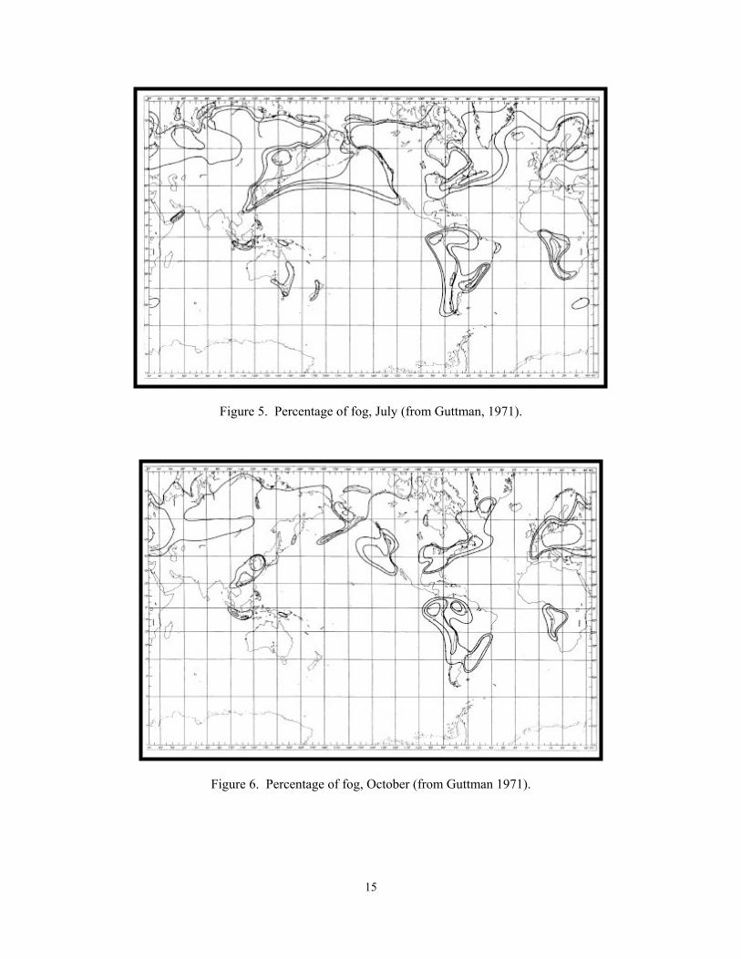
stability also play key roles. As can be seen from the distribution and variation of sea fog
in Figures 3 through 6, the fog favored regions are closely related to the locations of
major sea currents. In regions near the shore, such as in the eastern Yellow Sea, fog
often occurs where the cold and warm currents meet.
Sea surface temperature, in addition to sea current motion, is one of the most
important factors in the occurrence of sea fog. Figure 7 shows the mean sea surface
temperature in winter and summer around the southern Korean peninsula. There are a
few noticeable cold water regions depicted in the Yellow Sea during the early summer,
which are consistent with the high frequency of sea fog occurrences during this time.
The cold regions are characterized by shallow water under the strong tidal currents. The
shallow water and currents provides enough energy to mix the water column, resulting in
a relatively cold sea surface (Cho et al. 2000).

14
Figure 3. Percentage of fog, January (from Guttman, 1971).
Figure 4. Percentage of fog, April (from Guttman, 1971).
15
Figure 5. Percentage of fog, July (from Guttman, 1971).
Figure 6. Percentage of fog, October (from Guttman 1971).

16
A study on monthly mean frequencies of sea fog occurrences was conducted by
Cho et al. (2000) for nine coastal and 15 island stations around South Korea. The
average rate of occurrence showed that most sea fog occurs during the summer season
(Fig. 8), which is similar to the formation of sea fog around the United Kingdom, where
sea fog most commonly occurs in spring and early summer (Roach 1995). Cho et al.
(2000) also concluded the mean frequency of sea fog occurrence in the Yellow Sea is
higher than that of the Sea of Japan. Considering that both the Yellow Sea and Sea of
Japan are located at the same latitude, this difference most likely result from the
difference in sea surface temperatures.
The formation of sea fog cannot be determined solely from the evaluation of air
and sea surface temperatures. The maximum water vapor content at low levels and its
variation to surface water temperature must also be considered. As part of their sea fog
study, Cho et al. (2000) collected dew point temperature data and made comparisons to
sea surface temperatures. It was shown that the highest frequencies of fog (more than
30%) occurred when the difference between the dew point and sea surface temperature
was greater than 2º C. The frequency of fog increases with a higher difference between
the two values. It is generally accepted that higher dew points relative to the sea surface
temperature increases fog probability. If the dew point at the initial forecast time is less
than the coldest water temperature, the formation of fog is unlikely (5 WW 1979).

17
Kunsan
Longitude
Latit
ude
38
37
36
35
34
33
126 127124 125 129 130128 131
SST (° C)December
8
10
12
14
12
18
14
16
16
14
Kunsan
Longitude
Latit
ude
38
37
36
35
34
33
126 127124 125 129 130128 131
SST (° C)December
8
10
12
14
12
18
14
16
16
14
Kunsan
Longitude
Latit
ude
38
37
36
35
34
33
126 127124 125 129 130128 131
SST (° C)June
14
16
18
15
17
20
18
Kunsan
Longitude
Latit
ude
38
37
36
35
34
33
126 127124 125 129 130128 131
SST (° C)June
14
16
18
15
17
20
18
Figure 7. Mean sea surface temperature in (a) Dec and (b) Jun (adapted from Cho et al., 2000).

18
Longitude
Latit
ude
38
37
36
35
34
33
126 127124 125 129 130128 131
Kunsan
Sea FogFrequency (Days)January
0.0
0.0
0.41.6
Longitude
Latit
ude
38
37
36
35
34
33
126 127124 125 129 130128 131
Kunsan
Sea FogFrequency (Days)January
0.0
0.0
0.41.6
Longitude
Latit
ude
38
37
36
35
34
33126 127124 125 129 130128 131
Kunsan
Sea FogFrequency (Days)July
98
5
6
4
8
4
6
2
3
Longitude
Latit
ude
38
37
36
35
34
33126 127124 125 129 130128 131Longitude
Latit
ude
38
37
36
35
34
33126 127124 125 129 130128 131
Kunsan
Sea FogFrequency (Days)July
98
5
6
4
8
4
6
2
3
Figure 8. Mean frequency day of sea fog occurrence for (a) Jan and (b) Jul (adapted from Cho et al., 2000).

19
2.3 Physical Properties of Sea Fog
The density and visibility within sea fog depends on the number concentration
and size of fog droplets, as well as liquid water content (Binhua 1985). Neiburger and
Wurtele (1949) analyzed observations of visibility and relative humidity off the coast of
Los Angeles, California (Fig. 9). It is shown that, on average, the visibility decreases
almost uniformly as the relative humidity increases, with the decrease being due to
further condensation on the nuclei as air parcels approach saturation (Petterssen 1956).
Under certain conditions, Koschmieder (1924) proposed a formula for the visual
range V in a fog as:
V=[log(1/ε)] / πr2n (2)
where V is the visibility in centimeters, ε is the ratio of the difference in brightness
between the background and the object to the brightness of the background, n is the
number of drops per cubic centimeter, and r is the average radius of the drops in µm. In
most cases, ε is in the range of 0.01 to 0.02. It is seen from Eq. (2) that the visual range
is inversely proportional to the total projected area of the drops. Taking ε as a constant,
Eq. (2) may be written as:
V=[C rm] / wL (3)
where C is a constant, rm is the radius of the fog drop in µm, and wL is the liquid water
content in g/m3. For any given liquid water content, the visual range decreases as the
radius of the fog drops decrease. Cloud condensation nuclei are sparse in maritime air,
more plentiful in continental air, and abundant in urban air (Orgill 1993). Therefore, in

20
sea fog, where the drops are relatively large, the visual range would be larger than in a
city fog, where the drops are numerous and small.
Relative Humidity
Visi
bilit
y (m
iles)
40 80706050 10090
1
6
5
4
3
2
8
7
Relative Humidity
Visi
bilit
y (m
iles)
40 80706050 10090
1
6
5
4
3
2
8
7
Figure 9. Relation between visibility and relative humidity at Los Angeles Airport (adapted from Neiburger and Wurtele, 1949). The density of a sea fog expressed in terms of horizontal visibility depends not
only on the concentration of fog drops, but also on the liquid water content within the
fog. The distribution of liquid water in fog is relatively uniform over large horizontal
areas (Wallace and Hobbs 1977). The larger the liquid water content, the greater the
density of fog and the lower the visibility. Measurements of liquid water content were
taken during the period of June 15-23, 1951, by the Japanese research ship Yksek Maru
(Binhua 1985). The results showed that the liquid water content in sea fog averaged in a
range of 0.1 g/m3 to 2.0 g/m3. The average liquid water content range for land fog is 0.01
21
g/m3 to 1.0 g/m3. In general, the liquid water content in sea fog tends to be higher than
that for land fog.
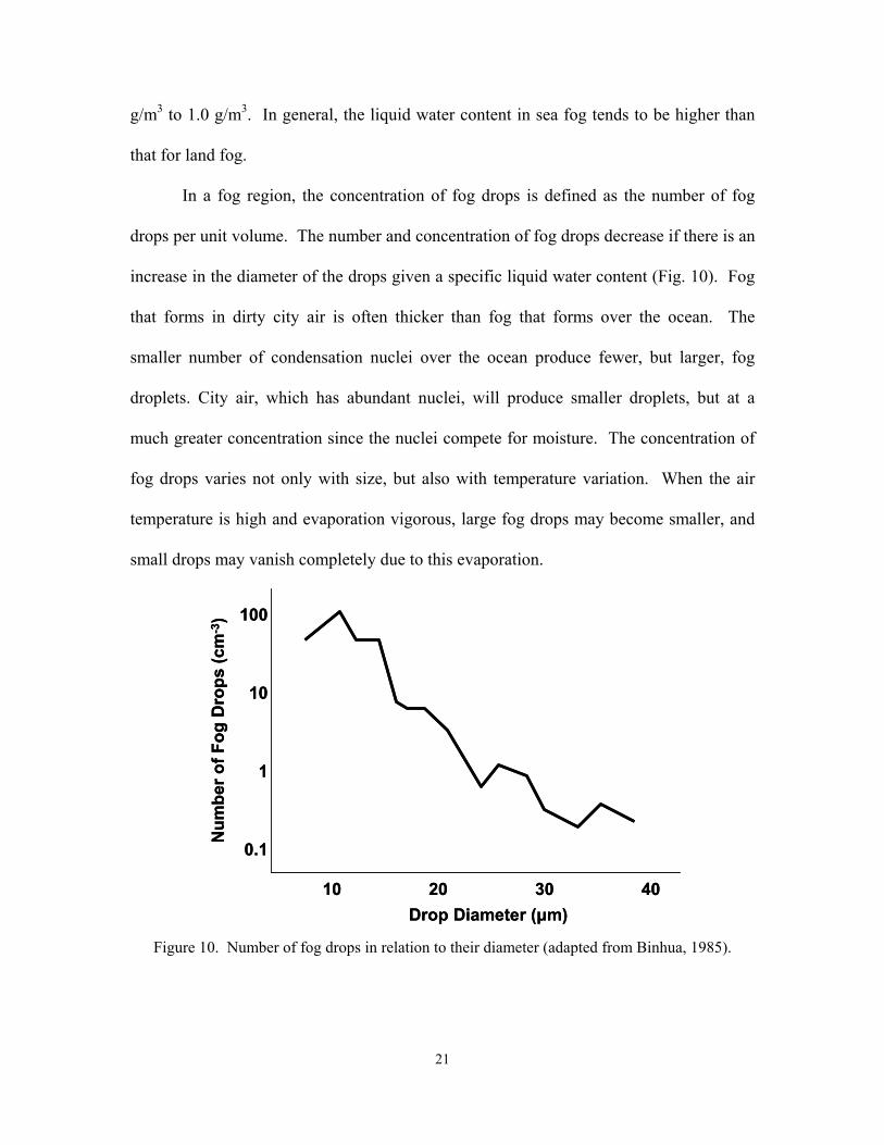
In a fog region, the concentration of fog drops is defined as the number of fog
drops per unit volume. The number and concentration of fog drops decrease if there is an
increase in the diameter of the drops given a specific liquid water content (Fig. 10). Fog
that forms in dirty city air is often thicker than fog that forms over the ocean. The
smaller number of condensation nuclei over the ocean produce fewer, but larger, fog
droplets. City air, which has abundant nuclei, will produce smaller droplets, but at a
much greater concentration since the nuclei compete for moisture. The concentration of
fog drops varies not only with size, but also with temperature variation. When the air
temperature is high and evaporation vigorous, large fog drops may become smaller, and
small drops may vanish completely due to this evaporation.
Drop Diameter (µm)
Num
ber o
f Fog
Dro
ps (c
m-3
)
10 20 30 40
0.1
1
10
100
Drop Diameter (µm)
Num
ber o
f Fog
Dro
ps (c
m-3
)
10 20 30 40
0.1
1
10
100
Figure 10. Number of fog drops in relation to their diameter (adapted from Binhua, 1985).

22
2.4 Dissipation
Fogs have a tendency to dissipate through heating. There is a marked diurnal
variation in the frequency of fogs, with a maximum in the early hours and a minimum in
the later afternoon. Naturally, a shallow fog will tend to burn off at a higher rate than a
deep fog. Most advection fogs are relatively deep, and the deeper ones will withstand
diurnal heating (Petterssen 1956). The same is true for fogs which have formed as a
result of advection followed by radiation. Since the variation of temperatures over
oceans is typically small, sea fogs are not as sensitive to diurnal variations as land fogs.
A light fog without much pollution will have an average liquid water content of
0.03 g/m3, while a dense fog may have a value in excess of 0.3 g/m3 (Petterssen 1956).
In order to dissipate a fog, the liquid water needs to be evaporated and the air temperature
must be increased so the water vapor resulting from evaporation can be accommodated in
the air. When the air temperature is high, only a slight increase is necessary to
accommodate the fog water, but a much greater temperature increase is needed with low
air temperatures. Fogs that occur at higher temperatures are more sensitive to diurnal
variations, while fogs over colder surfaces may persist all day.
One mechanism for dissipating advection fogs near coastlines is the advection
over warmer surfaces heated by solar radiation or heated artificially (Orgill 1993).
During the dissipation, the fog top moves upward, apparently in response to the increase
in turbulence that accompanies the development of an unstable temperature layer over the
warmer surface. However, fog movement over a warmer surface is not necessarily
sufficient for complete dissipation unless the heat from the surface is distributed
throughout the fog layer (Orgill 1993).

23
This past chapter described the geography of the region and its impacts to the
local climate at Kunsan AB. In addition, details on the dynamics of fog formation were
reviewed, with specific emphasis on the formation of sea fog. It was determined that
hydrological factors and weather conditions within the lower levels of the atmosphere are
the most significant for forecasting sea fog phenomena. Using this knowledge, data
containing these elements were analyzed for further study.
24
III. Data Collection and Review
3.1 Data Collection
The period of record (POR) examined in this research is from 1 January 1993
through 31 December 2002 in order to provide a 10 year sample size. Three different
sets of data were examined, with multiple variables within each data set. Surface weather
observations for Kunsan AB, ROK and sea surface temperature data for the Yellow Sea
were obtained from AFCCC databases. Upper air grid data for the Yellow Sea region
were obtained from the Navy Operational Global Atmospheric Prediction System
(NOGAPS) model, originating from the Fleet Numerical Meteorology and Oceanography
Center (FNMOC).
3.1.1 Kunsan AB, ROK Weather Observations. The Kunsan AB weather flight is
responsible for providing hourly Aviation Routine Weather Reports (METAR) for the
base airfield. The operating hours are seven days a week, 24 hours a day. The observing
site is located at 35°55'N, 126°37'E and is at an elevation of 29 feet. The POR for the
observations was 10 years, culminating in 101,249 total surface observations.
METAR is a routine scheduled observation as well as the primary observation
code used by the United States to satisfy requirements for reporting surface
meteorological data (AFMAN 2001). It contains a report of wind speed and direction,
visibility, sky condition, present weather, temperature, dew point, and altimeter setting.
Normally, points of observation are confined to an area within two statute miles of the
observing station, to include phenomena affecting the runway complex, drop zones or
landing zones. METAR observations normally reflect the conditions observed at, or seen

25
from, the usual point of observation within 15 minutes of the time ascribed to the
observation (AFMAN 2001).
The observations taken at Kunsan AB for the POR were obtained by a certified
weather observer, as opposed to an automated observing system. Limited observer
visibility to the northwest makes detection of advection fog difficult for the Kunsan
airfield (607th WS 2002). Therefore, while sea fog may have advected into the operating
area, documentation may not exist due to observer limitations.
3.1.2 Sea Surface Temperature (SST) Data. SST data were obtained from the
Surface Temperature (SFCTMP) model produced at the Air Force Global Weather
Central (AFGWC) and collected from the archives at AFCCC. The POR was from 1993
to 2002 and contains surface temperatures from 2816 grid points in the East Asian region.
Each grid point contains the surface temperature every three hours, for a total of 8
observations each day. For the purposes of this study, only four of the 2816 grid points
were used to correspond with the upper air data obtained from the NOGAPS model.
The SFCTMP model primarily supports the AFGWC Real-Time Nephanalysis
(RTNEPH) model at Offutt AFB, Nebraska. The RTNEPH model requires the surface
temperature data to make a cloud/no-cloud decision in its infrared thresholding algorithm
(Kopp 1995). SFCTMP runs separate analyses for the northern and southern
hemispheres, with each hemisphere mapped onto a polar stereographic grid with 1/8th-
mesh resolution. The array of gridpoints in each hemisphere is organized into 64 boxes,
laid out in an 8 x 8 array (Fig. 11).
Navy SSTs are received once every 12 hours at AFGWC from FNMOC over a
whole mesh grid (2.5 x 2.5 degree latitude/longitude). These data are ingested into the

26
Sea-Surface Processor, which is responsible for skin temperature analyses over all ice-
free water points. The data are then remapped over the smaller grid used by SFCTMP.
Figure 11. Polar stereographic grid for RTNEPH model (Department of the Air Force, 1986). The highlighted box is the area of interest for this study.
The SSTs then undergo a data quality check each six hour cycle. If any water point
contains a temperature colder than 270° K or warmer than 310° K, all SSTs in that

27
RTNEPH box are carried over from the previous cycle (Kopp 1995). This procedure
prevents unrealistic SSTs and avoids an excessively noisy analysis.
3.1.3 Upper Air Data. Upper air data for a POR from 1993 to 2002 was gathered
from the NOGAPS model output for the Yellow Sea region. NOGAPS data was obtained
on a 2.5 x 2.5 degree latitude and longitude grid, with analysis times of 00Z, 06Z, 12Z,
and 18Z daily. Data was collected from a variety of sources; such as land stations, ships,
buoys, aircraft, RAOB’s, and satellites. The data originates from FNMOC and is sent via
the Air Force Weather Agency (AFWA) to AFCCC.
The NOGAPS data for this study are considered to be reliable, considering the
techniques used to process the information. Optimum interpolation (OI) is an analysis
technique which takes into account three factors: distance between the observation and
the grid point, accuracy of the observing instrument, and expected accuracy of the first
guess (Department of the Air Force 1991). The first factor, distance between the
observation and grid point, is the foundation of nearly every numerical analysis scheme.
This factor assigns a weight to the observations around each grid point, with the weight
decreasing exponentially with distance. The closer the observation to the grid point, the
more weight it receives. Another advantage of OI is its ability to account for differences
between various instruments used to record observations. Every instrument is assigned
an expected error; the lower the expected error, the more weight the observation from
that instrument will have in the analysis. For example, an 850 mb temperature recorded
from a Rawinsonde Observation (RAOB) will have more influence in the analysis than
an 850 mb temperature

28
Less error assigned to RAOB thanSatellite at 850mb level
Less error assigned to RAOB thanSatellite at 850mb level
Figure 12. Sample of instrument errors (adapted from Department of the Air Force, 1991).
measured from a satellite (Fig. 12). The reverse would be true for temperature
measurements at levels above 250 mb. Finally, OI considers the expected accuracy of
the model’s first guess by producing error fields, estimating how accurate the analysis is
at each grid point. When more observations are available at a particular location, the
expected error will be lower, producing a more accurate analysis. For data rich areas
such as Europe and Asia, there will be less error than for data sparse areas like the South
Pacific. In addition, an inaccurate observation taken in one of the data rich areas will
have less impact on the analysis. The techniques used by OI increase the likelihood of
accurate analyses, and given the data rich region of this study, the data obtained for this
research can be considered reliable.

29
The data used for this research included temperature, dew point depression, wind
direction and wind speed for the surface, 1000 mb, 850 mb, 700 mb, 500 mb, and 300 mb
levels. These data include four points covering a square grid west of Kunsan:
122.5E/35N, 125E/35N, 122.5E/37.5N, and 125E/37.5N (Fig. 13). While data were
acquired from the surface through 300mb, only the lower atmospheric levels (surface to
850mb) were evaluated as predictors for this study, since sea fog is a lower atmospheric
phenomenon.
Kunsan
LONGITUDE
LATI
TUD
E
38
37
36
35
34
33 126 127124 125 129 130128 131122 123
A B
C D
Kunsan
LONGITUDE
LATI
TUD
E
38
37
36
35
34
33 126 127124 125 129 130128 131122 123
A B
C D
Figure 13. NOGAPS grid points used in this study.
3.2 Data Limitations
A major concern within this research is the relatively short POR of ten years.
There are a limited number of sea fog events which impacted Kunsan to analyze within
the surface observational data. While sea fog generally moves directly into Kunsan AB

30
from the southwest, it is possible for it to advect on land further to the west, impacting
other operating areas. On these occasions, a lack of observational data may occur due to
the limitations of the weather observer’s in detecting this phenomenon to the northwest,
where sea fog may have advected into the operating area, but not the airfield itself.
A second limitation with the research data is the NOGAPS grid. While the grid
box does cover a large portion of the Yellow Sea, there are no data points available for
the area immediately to the west of Kunsan. Since past authors have found SST is the
most significant predictor to sea fog formation, the lack of SST data directly west of
Kunsan may have an impact on determining an exact relationship between the predictor
variables and sea fog occurrence at Kunsan.
Finally, some of the data sets had incomplete, erroneous, or missing information.
Each of the data sets was carefully reviewed and corrections or deletions were made
based on the extent of the errors or absent information. Details on the processes used
during quality control are described in the next chapter.

31
IV. Methodology
This objective of this chapter is to examine the data and focus on producing
conditional climatology to aid forecasters in predicting low visibilities associated with
advective sea fog. The visibility categories evaluated are derived from the airfield
minimum categories used in the Operational Climatic Data Summary (OCDS) from
AFCCC (2000). Table 1 is a sample of the frequency for ceilings of 3000 feet and/or
visibility less than three statute miles. The table shows the percent frequency of
occurrence for each month during different times of the day in Local Standard Time
(LST). According to the OCDS, the highest probability of visibility dropping below
three miles occurs during June and July, which is consistent with the seasonal frequency
of sea fog. Typically for most locations, the highest probability of visibility dropping
below category is in the early to mid morning hours when the air temperature approaches
the dew point temperature. During June and July at Kunsan AB, the probabilities remain
relatively high throughout the day, which is common with a sea fog event.
Table 1. Percent frequency of ceiling/visibility less than 3000 feet/3 statute miles.
LST Jan Feb Mar Apr May Jun Jul Aug Sep Oct Nov Dec All 0-2 24 24 20 21 23 37 37 19 16 14 21 23 23 3-5 30 28 26 28 30 50 48 29 26 23 25 28 31 6-8 32 32 35 37 36 61 58 39 35 30 29 32 38
9-11 31 28 29 26 27 47 45 25 19 19 24 31 29 12-14 22 20 17 18 17 30 30 14 8 8 14 22 18 15-17 21 19 16 17 15 24 23 13 9 6 13 23 16 18-20 24 20 16 18 17 25 25 14 11 6 12 22 17 21-23 26 21 17 18 20 31 30 15 9 8 14 21 19 ALL 27 24 22 23 23 39 37 21 17 14 19 25 24

32
4.1 Data Examination
An examination of the data sets was necessary to determine a correlation between
the multiple weather parameters and the occurrence of sea fog. Prior to any statistical
studies being performed, extensive formatting was required on the data sets to ensure
they were usable for regression and data mining tests. This process involved extensive
manipulation of the three different sets of data: Kunsan AB surface observations,
NOGAPS upper air, and SST.
4.1.1 Surface Observational Database. Upon receiving the Kunsan AB surface
observations, quality control (QC) was performed on the data. The review was
conducted to determine any typographical errors or locate missing data. There were
several cases in 1996 and 1997 when visibility was less than seven statute miles, but
present weather condition data was missing. This particular category is important for this
research as it is necessary to distinguish between the causes of reduced visibilities,
whether it is due to fog, snow, rainshowers, etc. In the event of missing weather
information, present weather was manually inputted, as long as the inputted data was
supported by meteorological reasoning. For example, if the surface observations prior to
or after the observation in question contained reduced visibilities with mist (BR), or BR
was mentioned in the remarks section of the observation, then BR was inputted into the
data gap. If there were sections of data with excessive missing information, and there
were doubts as to the specific weather conditions, the observation was not used for this
study.
Upon completion of the QC, classification was completed on the present weather
conditions. The goal was to isolate those weather events where visibility was reduced

33
specifically by BR or fog (FG) from the snow, dust, or rain events. AFMAN 15-111
(2001) defines BR as “hydroscopic water droplets or ice crystals suspended in the
atmosphere that reduces visibility to less than 7 miles but equal to or greater than 5/8
mile.” FG is similar to BR, but with visibilities less than 5/8 mile. For the purposes of
simplifying the data set for this research, all weather events that are defined as either BR
or FG were reclassified as BR. Therefore, if a weather observation has ½ mile visibility
with present weather FG, it was reclassified as BR.
4.1.2 NOGAPS Upper Air Data. The second set of data contained the
atmospheric conditions for each of the four grid points depicted in Figure 13. The data
were provided every six hours beginning at 00Z for the ten year POR. QC was
performed on the data to located missing information and erroneous values. For any
missing data points, the information from the previous six hour model run was used to fill
the data gap. If data were missing for two or more consecutive model runs (12 or more
hours), the weather information for that time period was not used for the study. In
addition, any erroneous data located in the model run (a value of 5000 listed for dew
point depression) was replaced with the value from the previous six hour model run.
Upon completion of QC, the NOGAPS data were inputted into an Excel workbook, with
a specific sheet for each of the four grid points.
For the purposes of using the information in statistical and forecast decision tree
programs, it was necessary to merge the surface observations for Kunsan AB and the
NOGAPS data into one datasheet. NOGAPS had one set of values for 00Z, 06Z, 12Z,
and 18Z, while the surface observations contained a minimum of one entry per hour. In
34
order to synchronize the surface observations and NOGAPS data on one spreadsheet, the
surface observations were reduced from 24 or more a day to four. To accomplish this
task, the observations for 00Z, 06Z, 12Z, and 18Z were highlighted for study. The
weather information for the previous six hours from each of those highlighted
observations was evaluated to determine the average conditions. These average
conditions were inputted into the NOGAPS spreadsheet for each of the four time periods
of interest. In events of reduced visibilities due to fog, the minimum visibility to occur
during the six hour time period was used in the final spreadsheet. The Kunsan AB
surface observations were inputted into worksheets for each of the four NOGAPS grid
points.
The objective of this study was to produce a tool for providing a 24 hour forecast
of sea fog advecting into the Kunsan operating areas. In order to do this, the surface
observations were aligned with the NOGAPS data from the previous 24 hours. For
example, a 00Z surface observation for 2 January 2000 was inputted next to the 00Z
NOGAPS value for 1 January 2000. The purpose was to isolate the fog events, and relate
them to the atmospheric conditions which were occurring 24 hours previously, locating
parameters that may lead to sea fog formation.
4.1.3 SST Data. The final data set to be examined contained the SST from the
SFCTMP model, covering the 10 year POR. The original dataset contained values every
three hours with 2816 grid points covering the boxed area depicted in Figure 11. To
maintain consistency, the SST data were formatted for inclusion into the main NOGAPS
spreadsheet.

35
The first step was to focus on the SST grid points that were located in close
proximity to the four selected NOGAPS grid points. This involved reducing 2816 grid
points down to four by comparing the NOGAPS grid in Figure 11 to Figure 13. Next it
was necessary to ensure the time periods of the SST coincided with those already
selected for the NOGAPS and surface observations. This was a simple procedure
involving the removal of the 3Z, 9Z, 15Z, and 21Z from the datasheet, leaving the four
selected times of interest. The SST data were then inputted into the main spreadsheet,
with the data times and grid points aligned with the NOGAPS data. Any time period
with missing SST data was excluded from the study.
4.1.4 Results. The result for the first part of the objective was a thorough dataset
to be used for further statistical and data mining study. This dataset contains the
observed weather conditions at Kunsan AB aligned with upstream atmospheric and sea
surface temperature conditions for the preceding 24 hour time period. There is a separate
worksheet for each of the chosen grid points. The next step in the study involves
individually testing the target variable against the predictors for each of the four grid
points, and determining if a specific upstream location has a greater impact on sea fog
advection at Kunsan AB.
4.2 Statistical Analysis
Regression methods have become an integral component of any data analysis
concerned with describing the relationship between a target variable and one or more
predictor variables. The target variable for this research has only two qualitative
outcomes, and is represented by a binary indicator variable taking on values of 0

36
(visibility greater than 4800 meters) or 1 (visibility less than or equal to 4800 meters). In
many fields, the logistic regression model has become the standard method of analysis in
a categorical situation (Hosmer and Lemeshow 2000).
4.2.1 Logistic Regression. The difference between logistic regression and the
more familiar linear regression is reflected in the use of a binary outcome variable. Once
this difference is accounted for, the methods employed in an analysis using logistic
regression follow the same general principles used in linear regression.
The accuracy of a model is typically judged by the coefficient of determination
R2. R2 can be interpreted as the proportion of the variation of the predictand that is
described or accounted for by the regression (Wilks 1995). R2 values rarely reach unity,
and higher values typically indicate better effectiveness. However, this is not the case in
logistic regression. Hosmer and Lemeshow (2000) displayed several examples where the
value of R2 was relatively low when compared to R2 values typically encountered with
good linear regression models. Low R2 values in logistic regression are the norm and
present a problem when reporting their values to an audience accustomed to seeing linear
regression values. Therefore, R2 values were not considered with this research. For a
more detailed discussion on the specifics of logistic regression, reference Hosmer and
Lemeshow (2000).
4.2.2 Logistic Regression Results. It is important to determine if there is a
relationship between the target variable and the predictors early in the research. To do

37
this, initial testing was performed using a statistical software program from the SAS
Institute called JMP.
Nominal logistic regression was used when running the tests in JMP. Nominal
logistic regression estimates the probability of choosing one of the response levels as a
smooth function of the target variable. The fitted probabilities must be between 0 and 1,
and must sum to 1 across the response levels for a given target (SAS Institute 2000).
Two values calculated in JMP were considered when reviewing the significance
of the predictor variables to the target variable: Chi-Square and Prob>ChiSq. Chi-square
is the likelihood-ratio Chi-square test of the hypothesis that the model fits no better than
fixed response rates across the whole sample. Typically, the higher the value of Chi-
square, the more significant the predictor variable is to the target. Prob>ChiSq is the
observed significance probability, often called the p-value, for the Chi-square test. It is
the probability of getting, by chance alone, a Chi-square value greater than the one
computed. Models are often judged significant if this probability is below 0.05 (SAS
Institute 2000).
The data from each of the four grid points in the Yellow Sea were individually
inputted into JMP to test for the significance of the predictor variables to the formation of
sea fog. The target variable for these tests was Fog < 4800 meters. The predictor
variables used in JMP, along with a brief description of each variable, are listed in Table
2. For each grid point, there were thirteen predictor variables considered in the research.
The Chi-Square and p-value (Prob>ChiSq) results for the variables from each of the grid
points is displayed in Tables 3 through 6.

38
Table 2. Predictor variables used in JMP.
Predictor Description Deg C SST Sea surface temperature in degree Celsius SFCTEMP Surface temperature at grid point SFCDPD Surface dew point depression at grid point SFCDIR Surface wind direction at grid point SFCSPD Surface wind speed at grid point
1000TEMP 1000mb temperature at grid point 1000DPD 1000mb dew point depression at grid point 1000DIR 1000mb wind direction at grid point 1000SPD 1000mb wind speed at grid point 850TEMP 850mb temperature at grid point 850DPD 850mb dew point depression at grid point 850DIR 850mb wind direction at grid point 850SPD 850mb wind speed at grid point
Table 3. JMP results for Grid Point A.
Term Chi-Square p-value Deg C SST 26.24 <0.0001 SFCTEMP 0.05 0.8166 SFCDPD 21.65 <0.0001 SFCDIR 8.20 0.0042 SFCSPD 3.45 0.0631
1000TEMP 4.04 0.0445 1000DPD 8.58 0.0034 1000DIR 8.57 0.0034 1000SPD 36.66 <0.0001 850TEMP 17.63 <0.0001 850DPD 44.66 <0.0001 850DIR 4.33 0.0375 850SPD 27.69 <0.0001
Reviewing the information in Table 3, it can be seen that Deg C SST, 1000SPD,
850SPD, and 850DPD are the most significant predictors for grid point A. The overall
Chi-square calculated for this location was 950.2238, with a p-value of <0.0001. This
indicates there is a low probability of getting a higher Chi-square by chance alone.

39
Table 4. JMP results for Grid Point B.
Term Chi-Square p-value Deg C SST 46.42 <0.0001 SFCTEMP 0.05 0.8275 SFCDPD 6.53 0.0106 SFCDIR 9.69 0.0019 SFCSPD 5.94 0.0148
1000TEMP 0.02 0.8915 1000DPD 66.74 <0.0001 1000DIR 6.25 0.0124 1000SPD 26.40 <.0001 850TEMP 2.99 0.0840 850DPD 20.04 <0.0001 850DIR 0.70 0.4018 850SPD 10.55 0.0012
In Table 4, Deg C SST was an important predictor, as well as 1000DPD,
1000SPD, and 850DPD. The overall Chi-square value was 907.9326 with a p-value of
<0.0001. For grid point C shown in Table 5, 850DPD had the highest value, followed by
SFCDPD and Deg C SST. The overall Chi-square was 1072.539 and the p-value was
<0.0001.
Table 5. JMP results for Grid Point C.
Term Chi-Square p-value Deg C SST 48.53 <0.0001 SFCTEMP 0.11 0.7364 SFCDPD 51.43 <0.0001 SFCDIR 23.81 <0.0001 SFCSPD 0.40 0.5273
1000TEMP 8.20 0.0042 1000DPD 2.72 0.0994 1000DIR 0.01 0.9307 1000SPD 19.79 <0.0001 850TEMP 32.12 <0.0001 850DPD 80.03 <0.0001 850DIR 0.49 0.4838 850SPD 30.10 <0.0001

40
Table 6. JMP results for Grid Point D.
Term Chi-Square p-value Deg C SST 82.71 <0.0001 SFCTEMP 2.52 0.1121 SFCDPD 34.22 <0.0001 SFCDIR 14.86 0.0001 SFCSPD 0.17 0.6792
1000TEMP 8.40 0.0037 1000DPD 40.42 <0.0001 1000DIR 0.06 0.8069 1000SPD 75.41 <0.0001 850TEMP 20.87 <0.0001 850DPD 36.58 <0.0001 850DIR 3.83 0.0503 850SPD 0.48 0.4875
Table 6 shows that Deg C SST is once again an important predictor, along with
1000DPD, 1000SPD and 850 DPD. The Chi-square value was 1146.565 with the p-value
once again <0.0001.
One final modeling test, stepwise logistic regression, was run in JMP with the
four difference datasets. Stepwise selection of variables is widely used in regression.
Employing a stepwise selection procedure can provide a fast and effective means to
screen a large number of variables, and to fit a number of logistic regression equations
simultaneously. Any stepwise procedure for selection or deletion of variables from a
model is based on a statistical algorithm that checks for the “importance” of variables,
and either includes or excludes them on the basis of a fixed decision rule. The
“importance” of a variable is defined in terms of a measure of the statistical significance
of the coefficient for the variable (Hosmer and Lemeshow 2000).
Stepwise logistic regression was performed in JMP for each of the datasets, with
the results shown in Table 7. The probability required to be used in the model was set at

41
0.05. Predictor variables with a p-value value greater than 0.05 will be excluded from the
model produced by stepwise regression. The variables are listed in order of importance.
In other words, the variables that contribute most to the target variable (formation of sea
fog) are shown from most significant to least significant. What these tables suggest is
that SST and the upper air predictors have an impact on the formation of sea fog.
Table 7. Results from stepwise logistic regression performed on JMP.
Grid Point A Grid Point B Grid Point C Grid Point D SFCDPD 1000DPD SFCDPD 1000DPD 1000SPD 1000SPD 850DPD 1000SPD 850DPD Deg C SST 1000SPD 850DPD SFCDIR 850DPD SFCDIR SFCDPD 850SPD 850TEMP 850SPD Deg C SST
850TEMP SFCSPD Deg C SST 850TEMP Deg C SST 850SPD 850TEMP SFCDIR 1000DPD SFCDPD 1000TEMP 1000TEMP 1000DIR SFCDIR 850DIR 1000DIR
1000TEMP
While using JMP has shown that each of the grid points has some predictor
variables that relate to the target variable, they do not provide a means for developing a
forecast decision tool. It is necessary to establish specific numerical criterion for the
predictor variables to aid forecasters in determining whether or not sea fog will advect
into the Kunsan AB region. To accomplish this goal, forecast decision trees are produced
from a software program designed by Salford Systems called Classification and
Regression Tree (CART) analysis, discussed in the next chapter.

42
V. CART Overview, Method, and Results
5.1 CART Overview
Classification and regression tree (CART) analysis is one of the main techniques
employed in data mining (Benz 2003). CART is a single procedure that can be used to
analyze either categorical (classification) or continuous (regression) data. A defining
feature of CART is that it presents its results in the form of decision trees. The tree
structure of the output allows CART to handle massively complex data while producing
diagrams that are easy to interpret.
The CART methodology is technically known as binary recursive partitioning
(Breiman et al. 1984). The process is binary because the root node is always split into
exactly two child nodes and recursive by treating the child nodes as root nodes and
repeating the process. In order to split a root node into two child nodes, CART operates
by determining a set of questions with “yes” or “no” answers that permit accurate
prediction or classification of cases. For example, the question may be:
Is TEMP <= 7°C?
For each case the question is used to split the node by sending the “yes” answers to the
left child node and the “no” answers to the right.
Once a best split is found, CART repeats the search process for each child node,
continuing recursively until further splitting is impossible or stopped. Splitting is
impossible if only one case remains in a particular node, or if all the cases in that node
have the same predictor variables. CART also allows splitting to be stopped if the node

43
has too few cases, with the default lower limit set at ten cases for this research. The total
number of splits is determined by multiplying the total number of predictors by the
amount of records in the data set. For example, if there are ten predictors and 1000
records, then there will be 10,000 different splits considered in formulating the optimal
tree.
Once the maximal tree is grown, CART determines the best tree by testing for
error rates or costs. With sufficient data, the simplest method is to divide the sample into
learning and test sub-samples. The learning sample is used to grow an overly large tree,
while the test sample is used to estimate the rate at which cases are misclassified. The
misclassification error rate is calculated for the largest tree and every sub-tree. The best
sub-tree is the one with the lowest or near-lowest cost.
5.1.1 Tree Splitting Methods. There are six different splitting functions available
in the classification analysis: Gini, Symmetric Gini, Entropy, Class Probability, Twoing,
and Ordered Twoing. The best known rules for binary recursive partitioning are Gini and
Twoing, which were the two methods employed for this research. Because each rule
represents a different philosophy as to the purpose of the decision tree, each may grow a
different style of tree.
The Gini rule looks for the largest class in the database, and strives to isolate it
from all other classes. For example, with two Classes, 0 and 1, the Gini rule would
immediately attempt to pull all the Class 0 records into one node. In theory, a perfect
split would leave two pure child nodes of Class 0 and Class 1. A pure decision tree is
attainable only in very rare circumstances; in most real-world applications, database

44
fields that clearly partition classes are not available. Gini will attempt to come as close to
this ideal as possible by focusing on one class at a time. It will always favor working on
the largest class in the node. Gini performance is frequently so good that it is the default
rule in CART.
The Gini split searches for the best separation that produces a high amount of
purity (homogeneity or lack of variety) in the node (Benz 2003). The Gini impurity
criterion for the dataset t is given by:
i(t) = 1 – S (4)
where S is the sum of the squared probabilities p(j / t) from each class. For a two class
example node with 50 observations, 40 in Class 0 and 10 in Class 1, the impurity
calculation would be written as follows:
i(t) = 1 – [(40/50)2 + (10/50)2] = 0.32 (5)
Therefore, the impurity calculated for the above sample node would be 32 percent.
An alternative splitting criterion in CART is the Twoing function, which operates
by separating the classes into two groups that add up to 50 percent of the data. The
concept is based on class separation rather than node heterogeneity. The objective is to
make the likelihood that a given class j case goes to the left as different as possible from
the probability that it goes to the right (Benz 2003). The function sums the absolute
value of the probability differences over all j classes, with the formula given as:
( ) ( )2
| |4
L RL R
j
p p p j t p j t
− ∑ (6)
where p(j | tL) and p(j | tR) are the probabilities of an object being distributed into Class j
given left and right terminal nodes respectively (Breiman et al. 1984).
45
The rationale for the Twoing function is quite different from that of Gini. For a
multi-class problem, Twoing operates by dividing the classes into two groups, gathering
similar classes together, and attempting to separate the two groups in the descendant
nodes. It thus treats every multi-class split as if it were a two-class problem.
For the two-class problem, such as this research, the Gini and Twoing criteria are
mathematically equivalent. The tree structures are the same, as is the overall predictive
tree accuracies. If there are multiple classes and the performances of the criteria differ
substantially, Gini tends to yield the better splits and therefore is the default in CART
(Salford Systems 2001).
5.1.2 Priors. To further assist the algorithm in making the best splits, the
researcher must inform CART of the nature of the categorical class distribution (Benz
2003). When data are gathered from samples stratified on the target variable, the class
proportions observed in the data may be far from the population proportions (Salford
Systems 2001). The method used for adjusting the analysis for this circumstance is
known as Priors.
Priors equal is the default setting used in CART, and treats the classes in the
sample as if they were uniformly distributed in the population regardless of the observed
sample proportions. With the priors equal setting, CART pays no attention to how rare a
class is in the dataset. Instead, CART looks at whether a given node is more or less rich
in that class as compared to the root node. This default setting frequently gives the most
satisfactory results because each class is treated as equally important for classification
accuracy (Salford Systems 2002). Another setting is priors data, which means the

46
probabilities of each class occurring match the total sample frequency (Benz 2003). The
other options provided in CART are priors mix, learn, test, and specify, which are not
evaluated for this research.
5.1.3 Pruning Trees. CART will continue to grow trees until it is not possible to
grow them any further, either because it is no longer able to split or until the maximum
node size is reached. Breimen et al. (1984) recommends letting the splits continue until
pure classification is achieved. This pure result, containing thousands of nodes and
thereby unrealistic to use in a climatological study, would then be pruned upwards
providing results that have a more meaningful interpretation.
5.1.4 Testing. The best tree is determined by estimating its expected cost.
Generally, using a separate test data set provides the most accurate assessment of the true
error rate of a sequence of trees, providing there are a sufficient number of test cases.
There are five testing options available in CART, two of which were used in this
research: cross validation and fraction of cases selected at random for testing.
5.1.4.1 Cross Validation. 10-fold cross validation is typically used when there is
insufficient data available for a test sample, typically less than 3,000 observations.
However, cross validation can also be useful when analyzing a dataset with a rare target
class, such as sea fog which is the target in this research. In this instance, the total
number of observations is well above 3,000, but the class of interest has only a small
proportion of records.

47
Using cross validation, CART grows a maximal tree on the entire learning
sample. This is the tree that will be pruned back. CART then proceeds by dividing the
learning sample into 10 roughly equal parts, each containing a similar distribution of the
target variable. CART takes the first nine parts of the data, constructs the largest possible
tree, and uses the remaining 1/10 of the data to obtain initial estimates of the error rate of
selected sub-trees. The same process is repeated on another 9/10 of the data while using
a different 1/10 part as the test sample. The process continues until each part of the data
has been held in reserve one time as a test sample. The results of the 10 mini-samples are
combined to form error rates for trees of each possible size (Salford Systems 2001).
5.1.4.2 Fraction of cases selected at random for testing. This option allows
CART to automatically separate a specified percentage of cases of data for testing
purposes. This method is only recommended when there are a minimum of 3,000
observations available within the data set. The data selected for testing is random, and
there is no way to find out which records were used for the learning data set and the test
data set.
5.1.5 Class Assignment. It is important to understand the methods used in CART
when assessing the class assignment for each particular node; the percent error
misclassification stems directly from class assignment. The probability of a record going
into the left child node with Class n is computed with Bayes’ Theorem:
( ) ( ) ( )( ) ( ) ( ) ( ) ( ) ( )
0 00
0 0 1 1 2 2
|| .
| | |p L n p n
p n Lp L n p n p L n p n p L n p n
=+ +
(7)
where nx is Class 0,1 or 2. When using priors equal, the probability of Class n is the
number of cases in the left node over the total number of cases for that class. Consider an

48
example with two classes calculated with priors equal. The distribution of each class for
the root and child nodes is shown as:
Root Left Right Class 0 10560 6633 3927 Class 1 2026 1714 312 Using Bayes’ Theorem, the within node probabilities are calculated as:
Left Right Class 0 0.426 0.707 Class 1 0.574 0.293
where the class assignment for the left node is 1 and 0 for the right node. All the records
not of the assigned class contained in the node are misclassified. The percent error
misclassification is the sum of the misclassifications per class of each terminal node of
the entire tree.
5.2 Cart Methodology and Results
Prior to the construction of the classification trees, the data were properly
formatted with the fog target variable reclassified from continuous to categorical values
(for details on formatting, see section 4.1). Table 8 shows a list of all the variables
considered for CART testing. The overall goal when testing the data is to find a decision
tree which yields 30 percent or less misclassification error rates for the Class 1 fog
variable.
Before running the primary tests on CART, it was determined to use only grid
point B for producing the forecast decision trees. Although some correlation was found
between the target variable and predictor variables for each of the four locations, grid

49
point B maintained some of the strongest correlations for each of the predictor variables.
It was decided to focus on the data from this particular point for developing forecast
decision trees.
5.2.1 Initial Classification Testing. The initial dataset used for this research was
for grid point B (see Fig. 13), which contained a total of 12,586 records. Given this
amount of data, there were over 100,000 splits possible when running classification trees
in CART. The initial Class 1 target variable established for this research included all
events with visibility less than or equal to 4800 meters and present weather coded as BR
(fog). This eliminated those weather events where visibility was reduced due to rain,
snow, or other weather phenomena. One significant limitation to this categorization is it
does not distinguish advection fog events from radiation fog events, which could have a
severe impact on the final outcome.
To begin the testing, the data set was run using the first 13 predictor variables
from Table 8 against the target variable Fog ≤ 4800. The number of observations for fog
events accounts for approximately 16 percent of the data; therefore, priors equal was
used for all the classification trees so each class would be treated as equally important.
Testing was performed twice, once with 10-fold cross-validation and another with
random sampling (20 percent of the data set aside for testing). The results from the Gini
and Twoing methods were compared during the initial test to confirm mathematical
equivalency. It is noted in Table 9 that there is not a difference in the relative cost
(percent error left unexplained by the decision tree) between Gini and Twoing, due to the
nature of this research as a two class problem. Therefore, Gini will be the primary

50
method used for the classification trees. The percent misclassification and percent
prediction success rates are documented in Tables 10 and 11, with the classification trees
produced through 10-fold cross-validation and random sampling depicted in Figures 14
and 15.
Table 8. List of predictor variables used for CART.
Predictor DescriptionDeg C SST Sea surface temperature in degree CelsiusSFCTEMP Surface temperature at grid pointSFCDPD Surface dew point depression at grid pointSFCDIR Surface wind direction at grid pointSFCSPD Surface wind speed at grid point
1000TEMP 1000mb temperature at grid point1000DPD 1000mb dew point depression at grid point1000DIR 1000mb wind direction at grid point1000SPD 1000mb wind speed at grid point850TEMP 850mb temperature at grid point850DPD 850mb dew point depression at grid point850DIR 850mb wind direction at grid point850SPD 850mb wind speed at grid pointDP-SST Difference between dew point and SSTAT-SST Difference between air temperature at SST
RKJKDIR Wind direction at Kunsan ABRKJKSPD Wind speed at Kunsan AB
Table 9. Initial relative cost comparison for Grid B data set.
Gini Twoing Cross Validation 0.690 0.690 Random Testing 0.712 0.712
Table 10. 10-fold cross-validation misclassification rates for Grid B data set.
Class Total Cases Learn Data Error
Test Data Error
Learn Data Success
Test Data Success
0 10560 34.53% 34.37% 65.5% 65.6% 1 2026 31.15% 34.60% 68.9% 65.4%

51
Table 11. Random sampling misclassification rates for Grid B data set.
Class Total Cases Learn Data Error
Test Data Error
Learn Data Success
Test Data Success
0 8414 40.56% 41.89% 59.4% 58.1% 1 1613 25.67% 29.30% 74.3% 70.7%
The percent error misclassification rate for 10-fold cross-validation of Class 1, the
fog target variable, is 31.15% and 34.60% for learn and test data respectively. The
misclassification rates of Class 1 for random sampling testing were lower at 25.67% and
29.30%. As indicated from Table 9, the overall relative costs associated with random
sampling for this data set is higher, indicating a higher error rate covering all the data. It
is noted that Class 0 events have better results with 10-fold cross validation and Class 1
events have better results with random sampling. With the smaller percentage error rates
associated with Class 1 individually, it would seem the random sampling is an acceptable
test to use with this data set since classifying Class 1 events is the primary goal.
Figure 14 displays the classification tree produced from 10-fold cross-validation.
It is important to recognize that four of the root nodes had the same splitting criteria and
ranked in the same order of importance that was determined from the stepwise regression
performed on JMP (Table 7): 1000DPD, 1000SPD, Deg C SST and 850DPD. Similar
results from two statistical programs give confidence that these particular predictor
variables are of importance to the forecasting of fog events.
Figure 15 is the decision tree for the same data set using the random sampling
method. From Table 9, the overall relative cost was higher for this test, but the fog event
misclassification was lower. One thing to observe from the decision tree is the similarity

52
in split criteria for nodes 1 through 6 for each of the methods. The predictor variables are
the same for those particular nodes, although the specific split criteria (ex. 1000DPD ≤
6.250 versus 1000DPD ≤ 5.050) differ somewhat. In random sampling, a slightly higher
percentage of Class 1 fog events are split to the right of the tree from node 1 to node 8,
resulting in further splitting on that side of tree that did not occur with 10-fold cross-
validation. This percentage is still fairly minor when compared to the number of events
on the left side of the decision tree, which is where the primary focus will be.
Upon studying the split criteria from the first two trees, a potential problem with
the arrangement of the wind data was observed for node 5 and terminal nodes 2 and 3.
The split criterion for these terminal nodes was 850DIR, the 850 mb wind direction. The
winds were split at 850DIR ≤ 293.500° and 850DIR ≤ 289.500° for Figure 14 and Figure
15 consecutively. The wind direction is arranged around a 360° circle as depicted in
Figure 16. As can be seen from the shaded area of the graph, any winds that would be
less than 293.5° could fall within quadrants I, II, III or part of IV. Since this covers such
a large spectrum of values, the splitting of node 5 would only be of minimal use. The
method employed to overcome this dilemma was to review the data, and determine if
there were any sections of wind that could be deleted from the data set.
5.2.2 Testing with the removal of 0° through 135° NOGAPS winds. By reviewing
the complete data set, it was determined that observations with winds from the northeast
at grid point B could be deleted from the data set, with the assumption those winds would
advect sea fog away from the Kunsan operating area. Observations with SFCDIR,
1000DIR, and 850DIR NOGAPS values between 0° and 135° accounted for 35 percent
of

53
DEG_C_SST <= 22.100
TerminalNode 1
Class = 1Class Cases %
0 2505 71.01 1022 29.0
B850DIR <= 293.500
TerminalNode 2
Class = 0Class Cases %
0 849 89.81 96 10.2
B850DIR > 293.500
TerminalNode 3
Class = 1Class Cases %
0 97 72.91 36 27.1
B850DPD <= 6.850
Node 5Class = 0
B850DIR <= 293.500Class Cases %
0 946 87.81 132 12.2
B850DPD > 6.850
TerminalNode 4
Class = 1Class Cases %
0 388 73.81 138 26.2
DEG_C_SST > 22.100
Node 4Class = 1
B850DPD <= 6.850Class Cases %
0 1334 83.21 270 16.8
B1000SPD <= 12.500
Node 3Class = 1
DEG_C_SST <= 22.100Class Cases %
0 3839 74.81 1292 25.2
DEG_C_SST <= 22.300
TerminalNode 5
Class = 1Class Cases %
0 656 76.71 199 23.3
DEG_C_SST > 22.300
TerminalNode 6
Class = 0Class Cases %
0 335 91.81 30 8.2
SFCDPD <= 2.750
Node 7Class = 1
DEG_C_SST <= 22.300Class Cases %
0 991 81.21 229 18.8
SFCDPD > 2.750
TerminalNode 7
Class = 0Class Cases %
0 1803 90.31 193 9.7
B1000SPD > 12.500
Node 6Class = 0
SFCDPD <= 2.750Class Cases %
0 2794 86.91 422 13.1
B1000DPD <= 6.250
Node 2Class = 1
B1000SPD <= 12.500Class Cases %
0 6633 79.51 1714 20.5
B1000DPD > 6.250
TerminalNode 8
Class = 0Class Cases %
0 3927 92.61 312 7.4
Node 1Class = 0
B1000DPD <= 6.250Class Cases %
0 10560 83.91 2026 16.1
Figure 14. Forecast decision tree using Gini, 10-fold cross-validation. In node 1, the second line contains the class designation; the third line is the conditional statement. A yes response follows the next level into the left node, while a no response follows down a level to the right node.

54
DEG_C_SST <= 23.200
TerminalNode 1
Class = 1Class Cases %
0 1535 68.81 696 31.2
B850DIR <= 289.500
TerminalNode 2
Class = 0Class Cases %
0 580 89.21 70 10.8
B850DIR > 289.500
TerminalNode 3
Class = 1Class Cases %
0 83 72.21 32 27.8
B850DPD <= 9.650
Node 5Class = 0
B850DIR <= 289.500Class Cases %
0 663 86.71 102 13.3
B850DPD > 9.650
TerminalNode 4
Class = 1Class Cases %
0 64 62.71 38 37.3
DEG_C_SST > 23.200
Node 4Class = 1
B850DPD <= 9.650Class Cases %
0 727 83.91 140 16.1
B1000SPD <= 11.500
Node 3Class = 1
DEG_C_SST <= 23.200Class Cases %
0 2262 73.01 836 27.0
SFCDPD <= 2.950
TerminalNode 5
Class = 1Class Cases %
0 720 77.31 211 22.7
SFCDPD > 2.950
TerminalNode 6
Class = 0Class Cases %
0 861 87.41 124 12.6
DEG_C_SST <= 24.100
Node 7Class = 1
SFCDPD <= 2.950Class Cases %
0 1581 82.51 335 17.5
DEG_C_SST > 24.100
TerminalNode 7
Class = 0Class Cases %
0 374 94.01 24 6.0
B1000SPD > 11.500
Node 6Class = 0
DEG_C_SST <= 24.100Class Cases %
0 1955 84.51 359 15.5
B1000DPD <= 5.050
Node 2Class = 1
B1000SPD <= 11.500Class Cases %
0 4217 77.91 1195 22.1
B
C
Node 1Class = 0
B1000DPD <= 5.050Class Cases %
0 8414 83.91 1613 16.1
Figure 15. Forecast decision tree using Gini, random sampling. With random sampling, only 80% of the observations are used to produce the decision tree, as compared to 100% of the observations from 10-fold cross-validation.

55
DEG_C_SST > 24.100
TerminalNode 7
Class = 0Class Cases %
0 374 94.01 24 6.0
500
.100
55
B1000SPD <= 10.500
TerminalNode 8
Class = 1Class Cases %
0 1011 82.01 222 18.0
B1000SPD > 10.500
TerminalNode 9
Class = 0Class Cases %
0 454 90.61 47 9.4
B1000DPD <= 8.450
Node 10Class = 0
B1000SPD <= 10.500Class Cases %
0 1465 84.51 269 15.5
B1000DPD > 8.450
TerminalNode 10Class = 0
Class Cases %0 902 92.51 73 7.5
B1000SPD <= 13.500
Node 9Class = 0
B1000DPD <= 8.450Class Cases %
0 2367 87.41 342 12.6
B1000SPD > 13.500
TerminalNode 11Class = 0
Class Cases %0 1830 96.01 76 4.0
B1000DPD > 5.050
Node 8Class = 0
B1000SPD <= 13.500Class Cases %
0 4197 90.91 418 9.1
Node 1Class = 0
B1000DPD <= 5.050Class Cases %
0 8414 83.91 1613 16.1
Figure 15. (Continued).

56
the total data set, and 36 percent of all fog events (including radiation fog). Those
observations were deleted from the initial data set, renamed as “Test 2”, and another set
of tests were conducted with 10-fold cross-validation and random sampling, with the
results displayed in Tables 12 through 14.
90°270°
180°
360°
293.5° I
IIIII
IV
90°270°
180°
360°
293.5°
90°270°
180°
360°
293.5° I
IIIII
IV
Figure 16. Wind circle diagram. The wind data is given in degrees, with the numerical value giving the direction the wind is moving from. The top of the graph is north, and begins with 0°, moving about the circle in a clockwise direction. Quadrant I is all winds from the northeasterly direction, quadrant II southeasterly, quadrant III southwesterly, and quadrant IV northwesterly, completing the circle at 360° north.
Table 12. Relative cost comparison for Test 2 Grid B data set.
Gini Twoing Cross Validation 0.645 0.645 Random Testing 0.691 0.691

57
Table 13. 10-fold cross-validation misclassification rates for Test 2 Grid B data set.
Class Total Cases Learn Data Error
Test Data Error
Learn Data Success
TestData Success
0 6877 35.87% 35.61% 64.1% 64.4% 1 1300 20.46% 28.85% 79.5% 71.2%
Table 14. Random sampling misclassification rates for Test 2 Grid B data set.
Class Total Cases Learn Data Error
Test Data Error
Learn Data Success
Test Data Success
0 5465 30.69% 31.94% 69.3% 68.1% 1 1039 21.37% 37.16% 78.6% 62.8%
As indicated by Table 12, the Gini and Twoing methods once again produced
identical relative cost comparisons; therefore, the Gini method was used for all further
testing. From Table 13, the percent misclassification rate for 10-fold cross-validation of
Class 1 events is 20.46% for learn data and 28.85% for test data. This is an improvement
from the initial forecast decision tree in Table 10 of 34% for learn data and 17% for the
test data from the initial testing. From the random sampling testing results shown in
Table 14, the percent misclassification for learn and test data was 21.37% and 37.16%,
with an improvement of 16% for the learn data set. However, there was an 8% increase
in the number of Class 1 events misclassified when comparing the test data against the
learn data set when building the tree. This indicates the removal of the winds increased
the overall quality of the forecast decision tree, but for this particular data set, 10-fold
cross-validation provides better results than random sampling. 10-fold cross validation is
the preferred testing method due to the reduction in Class 1 cases after the removal of
wind data.
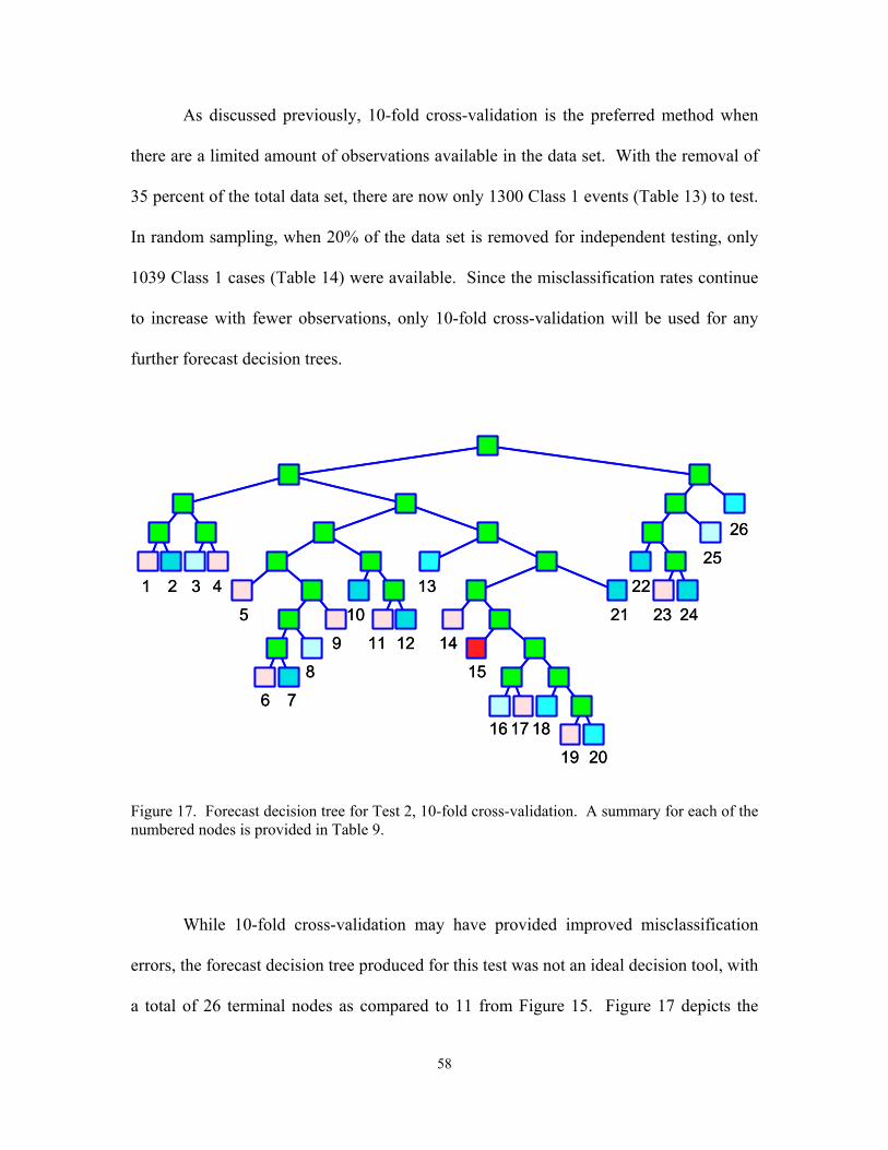
58
As discussed previously, 10-fold cross-validation is the preferred method when
there are a limited amount of observations available in the data set. With the removal of
35 percent of the total data set, there are now only 1300 Class 1 events (Table 13) to test.
In random sampling, when 20% of the data set is removed for independent testing, only
1039 Class 1 cases (Table 14) were available. Since the misclassification rates continue
to increase with fewer observations, only 10-fold cross-validation will be used for any
further forecast decision trees.
1 2 3 4
5
6 7
8
9
10
11 12
13
14
15
16 17
19 20
18
23 24
25
26
21
221 2 3 4
5
6 7
8
9
10
11 12
13
14
15
16 17
19 20
18
23 24
25
26
21
22
Figure 17. Forecast decision tree for Test 2, 10-fold cross-validation. A summary for each of the numbered nodes is provided in Table 9.
While 10-fold cross-validation may have provided improved misclassification
errors, the forecast decision tree produced for this test was not an ideal decision tool, with
a total of 26 terminal nodes as compared to 11 from Figure 15. Figure 17 depicts the
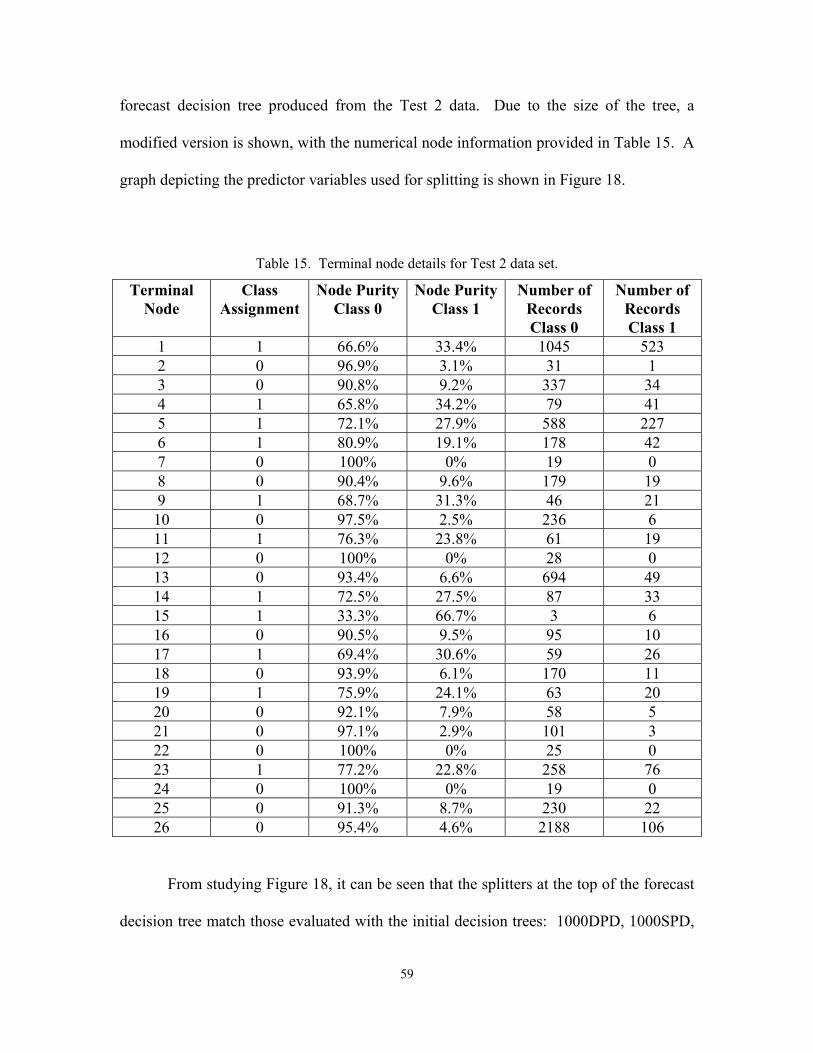
59
forecast decision tree produced from the Test 2 data. Due to the size of the tree, a
modified version is shown, with the numerical node information provided in Table 15. A
graph depicting the predictor variables used for splitting is shown in Figure 18.
Table 15. Terminal node details for Test 2 data set.
Terminal Node
Class Assignment
Node Purity Class 0
Node Purity Class 1
Number of Records Class 0
Number of Records Class 1
1 1 66.6% 33.4% 1045 523 2 0 96.9% 3.1% 31 1 3 0 90.8% 9.2% 337 34 4 1 65.8% 34.2% 79 41 5 1 72.1% 27.9% 588 227 6 1 80.9% 19.1% 178 42 7 0 100% 0% 19 0 8 0 90.4% 9.6% 179 19 9 1 68.7% 31.3% 46 21 10 0 97.5% 2.5% 236 6 11 1 76.3% 23.8% 61 19 12 0 100% 0% 28 0 13 0 93.4% 6.6% 694 49 14 1 72.5% 27.5% 87 33 15 1 33.3% 66.7% 3 6 16 0 90.5% 9.5% 95 10 17 1 69.4% 30.6% 59 26 18 0 93.9% 6.1% 170 11 19 1 75.9% 24.1% 63 20 20 0 92.1% 7.9% 58 5 21 0 97.1% 2.9% 101 3 22 0 100% 0% 25 0 23 1 77.2% 22.8% 258 76 24 0 100% 0% 19 0 25 0 91.3% 8.7% 230 22 26 0 95.4% 4.6% 2188 106
From studying Figure 18, it can be seen that the splitters at the top of the forecast
decision tree match those evaluated with the initial decision trees: 1000DPD, 1000SPD,
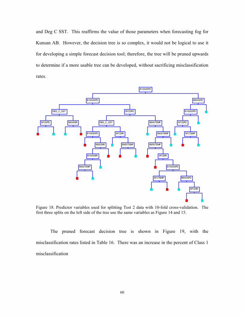
60
and Deg C SST. This reaffirms the value of those parameters when forecasting fog for
Kunsan AB. However, the decision tree is so complex, it would not be logical to use it
for developing a simple forecast decision tool; therefore, the tree will be pruned upwards
to determine if a more usable tree can be developed, without sacrificing misclassification
rates.
SFCDPD
B850DIR
DEG_C_SST
B850TEMP
B1000DIR
B850DIR
B1000DPD
B850TEMP
SFCDIR
DEG_C_SST
SFCTEMP
SFCDIR
B850SPD
B1000SPD
SFCDIR
B850TEMP
B850TEMP
B850TEMP
SFCDPD
B1000SPD
SFCTEMP
SFCDPD
B1000DPD
B850SPD
B1000DPD
Figure 18. Predictor variables used for splitting Test 2 data with 10-fold cross-validation. The first three splits on the left side of the tree use the same variables as Figure 14 and 15.
The pruned forecast decision tree is shown in Figure 19, with the
misclassification rates listed in Table 16. There was an increase in the percent of Class 1
misclassification

61
DEG_C_SST <= 23.700
TerminalNode 1
Class = 1Class Cases %
0 1076 67.31 524 32.8
B850DIR <= 290.000
TerminalNode 2
Class = 0Class Cases %
0 337 90.81 34 9.2
B850DIR > 290.000
TerminalNode 3
Class = 1Class Cases %
0 79 65.81 41 34.2
DEG_C_SST > 23.700
Node 4Class = 0
B850DIR <= 290.000Class Cases %
0 416 84.71 75 15.3
B1000SPD <= 9.500
Node 3Class = 1
DEG_C_SST <= 23.700Class Cases %
0 1492 71.41 599 28.6
DEG_C_SST <= 24.200
TerminalNode 4
Class = 1Class Cases %
0 1010 76.61 309 23.4
DEG_C_SST > 24.200
TerminalNode 5
Class = 0Class Cases %
0 325 92.91 25 7.1
SFCDPD <= 3.550
Node 6Class = 1
DEG_C_SST <= 24.200Class Cases %
0 1335 80.01 334 20.0
SFCDPD > 3.550
TerminalNode 6
Class = 0Class Cases %
0 1330 89.11 163 10.9
B1000SPD > 9.500
Node 5Class = 0
SFCDPD <= 3.550Class Cases %
0 2665 84.31 497 15.7
B1000DPD <= 6.250
Node 2Class = 1
B1000SPD <= 9.500Class Cases %
0 4157 79.11 1096 20.9
B1000DPD <= 8.950
TerminalNode 7
Class = 1Class Cases %
0 302 79.91 76 20.1
B1000DPD > 8.950
TerminalNode 8
Class = 0Class Cases %
0 230 91.31 22 8.7
B850SPD <= 12.500
Node 8Class = 0
B1000DPD <= 8.950Class Cases %
0 532 84.41 98 15.6
B850SPD > 12.500
TerminalNode 9
Class = 0Class Cases %
0 2188 95.41 106 4.6
B1000DPD > 6.250
Node 7Class = 0
B850SPD <= 12.500Class Cases %
0 2720 93.01 204 7.0
Node 1Class = 0
B1000DPD <= 6.250Class Cases %
0 6877 84.11 1300 15.9
Figure 19. Pruned forecast decision tree from Test 2 data using 10-fold cross-validation. Relative costs increased from 0.645 to 0.663 with an increase in learn data set misclassification from 20.46% to 26.92%.

62
rates from 20.46% to 26.92%, which falls within the maximum target error of 30%.
While this is tolerable, a more accurate decision tree is preferred for operational uses.
Table 16. Misclassification rates for pruned Test 2 data set, 10-fold cross-validation.
Class Total Cases Learn Data Error
Test Data Error
Learn Data Success
Test Data Success
0 6877 35.87% 37.21% 64.1% 62.8% 1 1300 26.92% 29.01% 73.1% 70.9%
5.2.3 Reclassified Sea Fog Target Variable. According to 607th Weather
Squadron (2002), there are some wind directions at Kunsan that are more conducive to
advective sea fog; it was determined it would be best to focus on those particular winds
for the next test. For Kunsan AB, typically winds from the south through northwest
result in the advection of sea fog into the operating area. Therefore, it was determined
that reclassifying the Class 1 fog target variable could possibly lead to more accurate
results. Going to the main data sheet, new criteria was established for the Class 1 target
variable. In addition to visibility less than or equal to 4800 meters and present weather
condition coded as BR, the surface winds reported at Kunsan AB must be from 140° to
340°. Only when all three of these criteria were met was the event classified as Class 1,
and the data set relabeled “Test 3” (for all observations) and “Test 4” (removal of 0°
through 135° upper air NOGAPS winds). This resulted in a reduction of Class 1 events
from 2,026 to 876 from the initial data set, and 1,300 to 681 from the Test 2 data set.
Due to the smaller number of Class 1 events, 10-fold cross-validation is the only method
used for the following forecast decision trees.

63
Table 17 shows the results for the Test 3 classification tree, with a
misclassification rate for learn data of 26.60% and test data of 30.25%, slightly out of the
target 30% error rate range. These results are from the classification tree with the lowest
relative costs. Further pruning of the tree yielded higher misclassification rates for the
Class 1 sea fog events; therefore, pruning of this decision tree was not performed.
Table 17. Misclassification rates for Test 3 data set, 10-fold cross-validation.
Class Total Cases Learn Data Error
Test Data Error
Learn Data Success
Test Data Success
0 11710 36.06% 37.48% 63.9% 62.5% 1 876 26.60% 30.25% 73.4% 69.8%
The most significant feature to note from the forecast decision tree produced from
the newly categorized target (Fig. 20) is the change in importance for the predictor
variables. In the decision trees produced from the initial data set and Test 2 data, the
primary parameters of interests were 1000DPD, 1000SPD and Deg C SST, regardless of
the testing method employed. With the updated target variable, the most significant
predictor variables are now 850TEMP, SFCDPD, SFCTEMP and 1000SPD. Using the
JMP software program to run logistic stepwise regression tests on the new target variable
yielded similar results. The top parameter considered by stepwise regression to be of
importance when building the model is 850TEMP, which does match the results from
CART. The other parameters determined by JMP in order of importance were Deg C
SST, 1000DPD, 1000SPD and SFCTEMP. The order does differ from the CART output,

64
B850TEMP <= 0.890TerminalNode 1
Class = 0Class Cases %
0 3517 97.71 84 2.3
SFCSPD <= 8.500TerminalNode 2
Class = 1Class Cases %
0 388 88.41 51 11.6
SFCSPD > 8.500TerminalNode 3
Class = 0Class Cases %
0 279 95.51 13 4.5
B1000DIR <= 104.500Node 5
Class = 1SFCSPD <= 8.500Class Cases %
0 667 91.21 64 8.8
B1000DIR > 104.500TerminalNode 4
Class = 1Class Cases %
0 1672 83.21 338 16.8
SFCTEMP <= 24.090Node 4
Class = 1B1000DIR <= 104.500Class Cases %
0 2339 85.31 402 14.7
B850DIR <= 222.500TerminalNode 5
Class = 0Class Cases %
0 524 97.01 16 3.0
B850DIR > 222.500TerminalNode 6
Class = 1Class Cases %
0 432 89.31 52 10.7
SFCTEMP > 24.090Node 6
Class = 0B850DIR <= 222.500Class Cases %
0 956 93.41 68 6.6
SFCDPD <= 3.350Node 3
Class = 1SFCTEMP <= 24.090Class Cases %
0 3295 87.51 470 12.5
B1000DPD <= 8.350TerminalNode 7
Class = 1Class Cases %
0 1203 89.81 137 10.2
B1000SN
ClB1000DClass C
01
B850TEMP > 0.890Node 2
Class = 1SFCDPD <= 3.350Class Cases %
0 8193 91.21 792 8.8
Node 1Class = 0
B850TEMP <= 0.890Class Cases %
0 11710 93.01 876 7.0
Figure 20. Forecast decision tree produced from Test 3 data, 10-fold cross-validation. This decision tree reclassifies the target, distinguishing all fog events from those events which are assumed to be specifically advective sea fog. Note that unlike prior decision trees, most of the Class 1 events now split to the right rather than the left of node 1.

65
B1000DPD <= 8.350TerminalNode 7
Class = 1Class Cases %
0 1203 89.81 137 10.2
B1000DPD > 8.350TerminalNode 8
Class = 0Class Cases %
0 342 95.51 16 4.5
B1000SPD <= 7.500Node 8
Class = 1B1000DPD <= 8.350Class Cases %
0 1545 91.01 153 9.0
SFCDIR <= 124.500TerminalNode 9
Class = 0Class Cases %
0 325 95.91 14 4.1
SFCDIR > 124.500TerminalNode 10
Class = 1Class Cases %
0 528 89.01 65 11.0
SFCDIR <= 338.500Node 12
Class = 1SFCDIR <= 124.500Class Cases %
0 853 91.51 79 8.5
SFCDIR > 338.500TerminalNode 11
Class = 0Class Cases %
0 142 97.91 3 2.1
SFCTEMP <= 27.590Node 11
Class = 1SFCDIR <= 338.500Class Cases %
0 995 92.41 82 7.6
SFCTEMP > 27.590TerminalNode 12
Class = 0Class Cases %
0 80 100.01 0 0.0
SFCDPD <= 4.850Node 10
Class = 1SFCTEMP <= 27.590Class Cases %
0 1075 92.91 82 7.1
SFCDPD > 4.850TerminalNode 13
Class = 0Class Cases %
0 2278 96.31 87 3.7
B1000SPD > 7.500Node 9
Class = 0SFCDPD <= 4.850Class Cases %
0 3353 95.21 169 4.8
SFCDPD > 3.350Node 7
Class = 0B1000SPD <= 7.500Class Cases %
0 4898 93.81 322 6.2
792 8.8
Figure 20. (Continued).

66
although SFCTEMP and 1000SPD are considered important predictors at the top of each
model.
One thing to note when studying the number of Class 1 cases contained in the
nodes is that some of them have a close to even split. For example, node 7 splits into
node 8 and node 9 based on 1000SPD criteria. In this instance, 153 cases go to node 8,
while 169 cases are split into node 9. With only a difference of 16 cases, this would
seem to be relatively weak splitting criteria, with minor value to the research.
Another major limitation with this particular forecast decision tree is the wind
direction splitting criteria. This particular data set maintained the original observational
database, including wind directions from the complete 360° wind circle. This results in
the same splitting weakness that occurred with the initial data set. Therefore, further
testing was completed with the modified NOGAPS wind data.
Ten-fold cross-validation was performed on Test 4 data, sea fog events without
NOGAPS winds from 0° to 135°. The relative cost for this decision tree was 0.597, the
lowest of all the trees produced thus far. The misclassification results are displayed in
Table 18, with the forecast decision tree in Figure 21, node report in Table 19, and
splitting parameters in Figure 22.
Unlike the forecast decision tree produced from Test 3 data, it is possible to prune
the Test 4 tree into a more manageable forecast tool, with minimal negative impacts to
the misclassification rates. Table 20 shows the misclassification results for the pruned
tree, with Figure 23 representing the pruned forecast decision tree.

67
Table 18. Misclassification rates for Test 4 data set, 10-fold cross-validation.
Class Total Cases Learn Data Error
Test Data Error
Learn Data Success
Test Data Success
0 7496 34.11% 32.52% 65.9% 67.5% 1 681 17.62% 27.17% 82.4% 72.8%
The learn data set for Test 4 has the lowest misclassification rate seen in the
research, with 17.62% error. When running the test data against the forecast decision
tree produced from the learn data sets, error increases to 27.17%, but still within the
target of 30% maximum error. As with the forecast decision tree from Test 2, there are
18 terminal nodes which provides an unrealistic forecast decision tree for operational use.
The tree is shown in Figure 21, with a report of the terminal node data given in Table 19.
1
2
3 4
5
7 8
6
9
10
11
12
13
14 15 16 17
18
1
2
3 4
5
7 8
6
9
10
11
12
13
14 15 16 17
18
Figure 21. Forecast decision tree from Test 4 data, 10-fold cross-validation. A summary for each of the numbered nodes is provided in Table 13.

68
Table 19. Terminal node details for Test 4 data set.
Terminal Node
Class Assignment
Node Purity Class 0
Node Purity Class 1
Number of Records Class 0
Number of Records Class 1
1 0 97.8% 2.2% 2519 57 2 1 80.2% 19.8% 1425 352 3 0 97% 3% 558 17 4 1 66.7% 33.3% 8 4 5 1 84.4% 15.6% 76 14 6 1 88% 12% 309 42 7 1 88.2% 11.8% 180 24 8 0 95.3% 4.7% 204 10 9 0 98.9% 1.1% 90 1 10 0 100% 0% 53 0 11 0 98.4% 1.6% 121 2 12 1 81.9% 18.1% 384 85 13 0 96% 4% 333 14 14 0 100% 0% 37 0 15 1 82.1% 17.9% 165 36 16 0 97.6% 2.4% 249 6 17 1 71.4% 28.6% 10 4 18 0 98.4% 1.6% 775 13
The pruned forecast decision tree from Figure 23 reduces the number of nodes
from the right side of the tree, while increasing the misclassification rate by less than two
percent. This ensures the tree is more manageable as a decision tool, without sacrificing
accuracy. From studying the tree, it is noted that node 2 contains a total of 624 Class 1
events, with a split of 387 into node 3 and 237 into node 4. Although there is a
difference of 150 cases, the splitting criteria does not discriminate between classes well.
From node 3 the splitting criteria is DEG C SST ≤ 23.000, resulting in a Class 1
terminal node 4. From the 237 Class 1 events in node 4, the split is 1000SPD to nodes 5
and 6, with a majority of the Class 1 events split into node 5. From node 5, the split

69
criteria is DEG C SST ≤ 23.000 (same as node 3), with the majority of Class 1 events
forming terminal node 4. Similar terminal node results for DEG C SST from different
branches of the decision tree allow a workable solution to the previously mentioned node
2 split.
SFCSPD
B850DIR
DEG_C_SST
SFCDPD
SFCTEMP
B850SPD
B850DPD
B850SPD
B1000TEMP
DEG_C_SST
B850TEMP
B850DIR
SFCTEMP
B1000DIR
B1000SPD
SFCDPD
B850TEMP
Figure 22. Predictor variables used for splitting Test 4 data with 10-fold cross-validation. Note that the first two splits of the decision tree use the same predictor variables as the Test 3 decision tree in Figure 20.
Table 20. Misclassification rates for pruned Test 4 data set, 10-fold cross-validation.
Class Total Cases Learn Data Error
Test Data Error
Learn Data Success
Test Data Success
0 7496 35.59% 34.99% 60.4% 65.0% 1 681 18.94% 28.63% 81.1% 71.4%

70
B850TEMP <= -0.210
TerminalNode 1
Class = 0Class Cases %
0 2519 97.81 57 2.2
DEG_C_SST <= 23.800
TerminalNode 2
Class = 1Class Cases %
0 1425 80.21 352 19.8
DEG_C_SST > 23.800
TerminalNode 3
Class = 0Class Cases %
0 642 94.81 35 5.2
SFCDPD <= 3.350
Node 3Class = 1
DEG_C_SST <= 23.800Class Cases %
0 2067 84.21 387 15.8
DEG_C_SST <= 23.000
TerminalNode 4
Class = 1Class Cases %
0 1341 89.11 164 10.9
DEG_C_SST > 23.000
TerminalNode 5
Class = 0Class Cases %
0 333 96.01 14 4.0
B1000SPD <= 12.500
Node 5Class = 1
DEG_C_SST <= 23.000Class Cases %
0 1674 90.41 178 9.6
SFCTEMP <= 15.790
TerminalNode 6
Class = 1Class Cases %
0 202 84.91 36 15.1
SFCTEMP > 15.790
TerminalNode 7
Class = 0Class Cases %
0 259 96.31 10 3.7
B1000DIR <= 269.000
Node 7Class = 1
SFCTEMP <= 15.790Class Cases %
0 461 90.91 46 9.1
B1000DIR > 269.000
TerminalNode 8
Class = 0Class Cases %
0 775 98.41 13 1.6
B1000SPD > 12.500
Node 6Class = 0
B1000DIR <= 269.000Class Cases %
0 1236 95.41 59 4.6
SFCDPD > 3.350
Node 4Class = 0
B1000SPD <= 12.500Class Cases %
0 2910 92.51 237 7.5
B850TEMP > -0.210
Node 2Class = 1
SFCDPD <= 3.350Class Cases %
0 4977 88.91 624 11.1
Node 1Class = 0
B850TEMP <= -0.210Class Cases %
0 7496 91.71 681 8.3
Figure 23. Forecast decision tree from pruned Test 4 data, 10-fold cross-validation. Note that the split from node 2 to nodes 3 and 4 only has a difference of 150 cases, resulting in a close split. It would seem that while SFCDPD is a split criterion, it is not a very decisive parameter.

71
5.2.4 Addition of new predictor variables. One more test was conducted using the
Test 4 data set, with the addition of two new predictor variables. According to Cho et al.
(2000), the difference between air temperature (AT) and SST, as well as the difference
between dew point (DP) and SST are important factors that affect the occurrence of sea
fog. These two parameters were calculated in the datasheet and run through the CART
program, using Gini and 10-fold cross-validation. The first forecast decision tree
produced has a relative cost of 0.604 and a total of 24 terminal nodes. The
misclassification rates are shown in Table 21, with the decision tree displayed in Figure
24, node report in Table 22, and splitter variables in Figure 25.
Table 21. Misclassification rates with AT-SST and DP-SST predictor variables.
Class Total Cases Learn Data Error
Test Data Error
Learn Data Success
Test Data Success
0 7496 31.96% 33.50% 68.0% 66.5% 1 681 17.62% 26.87% 82.4% 73.1%
Table 21 lists a misclassification rate for Class 1 events as 17.62% for learn data
and 26.87% for test data, which is similar to the rates calculated for the sea fog Test 4
data. Figure 24 shows there are 24 terminal nodes in the optimal tree, which makes this
an unrealistic tool for use in forecasting sea fog events. Figure 25 shows the splitting
variables used for the new decision tree. Although the misclassification rates are similar
from this test and the Test 4 data set, there is a significant difference in the splitting
variables from Figure 25 to those from Figure 22. The new predictor variable DP-SST
located in node 1 is now the primary splitter for the data set.

72
1
2
3
4 5
6
7
8
9
10
11
12 13
14
15
1617
19
20
18
23
24
21
22
1
2
3
4 5
6
7
8
9
10
11
12 13
14
15
1617
19
20
18
23
24
21
22
Figure 24. Forecast decision tree with AT-SST and DP-SST predictor variables. A summary for each of the numbered terminal nodes is provided in Table 16.
From reviewing the results from this latest test, the misclassification rates are
acceptable for developing a forecast tool, but the tree itself has two many terminal nodes
for adequate operational use. Therefore, the tree was pruned back to reduce the number
of nodes, and providing a reasonable forecast decision tree with the new predictor
variables. By pruning the tree upwards, the relative cost increased from 0.604 to 0.644,
but the Class 1 misclassification results did not differ significantly from the optimal tree,
as shown in Table 23.
The Class 1 test data error has an increase of near one percent for the pruned tree.
By using this particular forecasting decision tree, there is approximately a test data 72%
prediction success rate for forecasting advective sea fog for Kunsan AB. The decision
tree with the new predictor variables is shown in Figure 26.

73
Table 22. Terminal node details with new AT-SST and DP-SST predictor variable.
Terminal Node
Class Assignment
Node Purity Class 0
Node Purity Class 1
Number of Records Class 0
Number of Records Class 1
1 0 96.5% 3.5% 495 18 2 1 78.6% 21.4% 33 9 3 1 79.5% 20.5% 31 8 4 0 97.7% 2.3% 129 3 5 1 88% 12% 73 10 6 0 100% 0% 73 0 7 1 78.2% 21.8% 154 43 8 0 99.1% 4.7% 204 10 9 0 98.5% 1.5% 2605 41 10 1 83.8% 16.2% 109 21 11 1 81.8% 18.2% 45 10 12 0 94.9% 5.1% 409 22 13 1 70.6% 29.4% 12 5 14 0 100% 0% 75 0 15 1 81.1% 18.9% 163 38 16 0 97.4% 2.6% 227 6 17 1 81.3% 18.7% 1686 388 18 0 98.2% 1.8% 430 8 19 0 99.1% 0.9% 106 1 20 0 93.7% 6.3% 149 10 21 1 76.8% 23.2% 63 19 22 0 95.8% 4.2% 227 10 23 1 73% 27% 27 10 24 0 100% 0% 66 0
Studying the pruned decision tree from Figure 26 shows that the predictor
variable DP-SST is now the lead splitting criterion, as compared to 850TMP from Figure
23. The second split of importance for Class 1 events was Deg C SST, which already
proved to be a significant variable as shown in previous decision trees.
Reviewing all the tests and forecast decision trees produced for this research
problem, it is determined that the two most significant for the forecasting of sea fog are
the trees from Figure 23 and Figure 26. These two decision trees come from a data set

74
that had been filtered to remove winds that did little to contribute to the development of
sea fog. In addition, the target variable was formatted from the Kunsan AB surface
observations in a way such that the reduced visibility events that were not the direct
result
SFCTEMP
B850DPD
B1000DIR
B1000TEMP
DEG_C_SST
SFCTEMP
B850TEMP
B850DIR
B1000DIR
B850DIR
B850SPD
DEWPOINT
DP_SST
B1000TEMP
B850TEMP
DP_SST
AT_SST
AT_SST
SFCTEMP
SFCTEMP
B850DIR
DEG_C_SST
DP_SST
Figure 25. Forecast decision tree splitters with new predictor variables. Note that the primary split is based on the new variable DP-SST, while AT-SST is further down the right side of the tree.
Table 23. Misclassification rates for pruned tree with AT-SST and DP-SST variables.
Class Total Cases Learn Data Error
Test Data Error
Learn Data Success
Test Data Success
0 7496 39.91% 36.21% 60.1% 63.8% 1 681 18.21% 28.19% 81.8% 71.9%

75
B850TEMP <= -0.410
TerminalNode 1
Class = 0Class Cases %
0 495 96.51 18 3.5
SFCTEMP <= 15.590
TerminalNode 2
Class = 1Class Cases %
0 493 87.11 73 12.9
SFCTEMP > 15.590
TerminalNode 3
Class = 0Class Cases %
0 109 99.11 1 0.9
B850TEMP > -0.410
Node 4Class = 1
SFCTEMP <= 15.590Class Cases %
0 602 89.11 74 10.9
B850DIR <= 295.500
Node 3Class = 0
B850TEMP <= -0.410Class Cases %
0 1097 92.31 92 7.7
B850DIR > 295.500
TerminalNode 4
Class = 0Class Cases %
0 2605 98.51 41 1.5
DP_SST <= -9.360
Node 2Class = 0
B850DIR <= 295.500Class Cases %
0 3702 96.51 133 3.5
B1000TEMP <= 14.390
TerminalNode 5
Class = 1Class Cases %
0 813 89.41 96 10.6
B1000TEMP > 14.390
TerminalNode 6
Class = 0Class Cases %
0 227 97.41 6 2.6
B850TEMP <= 8.390
Node 7Class = 1
B1000TEMP <= 14.390Class Cases %
0 1040 91.11 102 8.9
B850TEMP > 8.390
TerminalNode 7
Class = 1Class Cases %
0 1686 81.31 388 18.7
DEG_C_SST <= 23.000
Node 6Class = 1
B850TEMP <= 8.390Class Cases %
0 2726 84.81 490 15.2
DEG_C_SST > 23.000
TerminalNode 8
Class = 0Class Cases %
0 1068 94.81 58 5.2
DP_SST > -9.360
Node 5Class = 1
DEG_C_SST <= 23.000Class Cases %
0 3794 87.41 548 12.6
Node 1Class = 0
DP_SST <= -9.360Class Cases %
0 7496 91.71 681 8.3
Figure 26. Forecast decision tree with AT-SST and DP-SST predictor variables. Note that the new variable DP-SST is the splitting criterion for node 1, with a majority of Class 1 events moving into the right side of the decision tree.

76
of sea fog were not classified as Class 1 events. Finally, these two particular trees had
the lowest misclassification results for Class 1 events when compared to all the tests
conducted.
The splitting rules established for the produced trees are to be verified with 24-
hour lead-time of the occurrence of sea fog at Kunsan AB. These rules have been
established through the CART program with 10 years of climatological analysis data.
The predictors yield a 72% accuracy rating, and should be used as a guide for a more
sound forecast decision of sea fog 24 hours in advance.

77
VI. Conclusions and Recommendations
6.1 Conclusions
The overall goal of this research was to determine a method for forecasting sea
fog events at Kunsan AB, with a 24-hour lead-time. The primary method used to satisfy
this objective was data mining with classification and regression tree analyses. This
research used observational data from Kunsan AB and analysis data from the NOGAPS
and SFCTMP models covering the Yellow Sea region.
The first objective was to perform a geographical and climatological overview of
the Kunsan AB region. Kunsan is a port city located in southwest Korea, bordered on the
west and south by the Yellow Sea. The close proximity to the water and seasonal
fluctuations of the Yellow Sea Current result in numerous advective sea fog events in the
area, particularly in the spring and summer months when cold water upwelling is
prevalent.
The second objective defined fog types and formation processes, and how they
relate to this region. The formation of sea fog is dependent on hydrological factors such
as sea current and sea surface temperature, as well as air temperature, humidity, and
wind. Advective sea fog is formed when warmer air moves over a cooler water surface,
such as when warmer air moves over the cold water upwelling off the coasts of southwest
Korea.
Third, the collection of sea surface temperature data, upper air data, and surface
observational data for Kunsan AB, as well as upstream locations (both over land and the
Yellow Sea), was necessary to continue the study. The three sets of data included
surface weather observations for Kunsan AB, sea surface temperature data for the Yellow

78
Sea (both obtained from AFCCC databases), and upper air grid data for the Yellow Sea
region covering four grid points (from the NOGAPS model).
For the fourth objective, formatting all the data was necessary in order to perform
statistical examinations. Since the target variable was defined categorically, logistic
regression (which works with a binary outcome variable) was the statistical method of
choice. These tests compared the correlation between the target variable (sea fog) and
the various predictor variables. Stepwise logistic regression was performed on JMP to
determine the importance of various predictor variables. The study was narrowed down
to one grid point of interest, which from initial testing had the most significant effect on
advective sea fog impacting Kunsan AB. The predictors were listed in order of
importance to the formation of fog, but more detailed information was needed to provide
a forecast decision tool to the 8th OSS/OSW at Kunsan AB.
To develop a forecast decision tool, the fifth objective was to use data mining
CART analysis on the data sets. Data mining was used to determine if there were
relationships between the target variable and predictor variables that was not evident
through standard statistical regression. Multiple tests were run, modifying the data sets
in an effort to produce the most effective forecast tool. The predictor variables used for
splitting in the initial forecast decision trees were similar to those variables determined
by JMP to be of most importance: 1000DPD, 1000SPD, DEG C SST, and 850DPD.
Upon changing the rules for categorizing the target variable, the key parameter of
importance as determined by JMP was 850TMP, which was the same result as the
decision tree produced by CART. A final test was performed by adding two new
predictor variables, which once again changed the splitting criteria. One of the new

79
variables, DP-SST was listed as the most significant in JMP, as well as the top splitting
criterion in CART.
The final objective was to develop forecast decision trees to assist in choosing the
best predictors for forecasting advective sea fog, and providing that product to the 8th
OSS/OSW at Kunsan AB. Beginning with the initial data set and eventually modifying
the target variable and adding two new predictors, a total of nine forecast decision trees
were produced.
The first decision tree produced a test data accuracy rating of 65.4%, well below
the standards set for this research. Upon modifying the wind data, the accuracy rating for
test data increased to 71.2%. The next decision tree of importance contained the
reclassified target variable, and produced an accuracy rating of 72.8%, but this tree was
too large to use operationally without producing a computerized forecast model. Upon
pruning the tree (Figure 23), the accuracy rating decreased to 71.4%, but still within
reasonable limits. A final tree was developed by adding two predictor variables and
pruning upwards (Figure 26), yielding an accuracy rating of 71.9%. It was determined
that the decision trees from Figure 23 and Figure 26 produced the best results, with an
almost equal prediction success of approximately 72%.
The forecast decision trees from Figures 23 and 26 contained the data set that
removed observations with SFCDIR, 1000DIR, and 850DIR NOGAPS values between
0° and 135°, which accounted for 35 percent of the total data set, and 36 percent of all
fog events (including radiation fog events). In addition, the target variable was
reclassified from the original “Fog ≤ 4800” to “Sea Fog”, which had the following
conditions: visibility less than or equal to 4800 meters, present weather condition coded
80
as BR, and the surface winds reported at Kunsan AB from 140° to 340°. This was done
in an effort to filter radiation fog events rather than advection sea fog occurrences.
It was determined to make two sea fog decision tree tools; one based off of each
of the selected CART forecast decision trees. Since each of the selected decision trees
produced an accuracy rating of approximately 72%, both should be tested for application
in real-time weather forecasting. The final Sea Fog Forecast Decision Trees are seen in
Appendices A and B. These rules are experimental and formulated as suggestive criteria
for developing more accurate sea fog forecasts. However, they are provided and
recommended for immediate operational use as they are developed from actual
observational data.
6.2 Recommendations
CART analyses used in this research provided insightful information into the
feasibility of providing forecasts by means of forecast decision trees. Given large
databases and a variety of predictors, accuracy ratings can be calculated for new methods
in forecasting which may not have been considered previously. However, given the
nature of data mining and as seen from the products produced in this research, CART
does not always yield one unambiguous method which can be used in forecast decisions.
Further research on this particular topic is desired in an effort to improve
accuracy ratings of the forecast decision trees. An extended POR will yield a greater
database for CART to work with, allowing a wider range of tests to be conducted within
the program, rather than just 10-fold cross-validation. In addition, the NOGAPS data
used for this research was on a 2.5 x 2.5 degree grid, whereas NOGAPS is now available
on a 1 x 1 degree grid. A wider range of data points in the region to the west of Kunsan

81
AB may provide a more accurate location from which to forecast the formation of
advective sea fog events.
Another recommendation for future research is to develop the forecasting
decision tree to include low level stratus conditions in addition to sea fog advecting into
the Kunsan operating area. On many occasions low stratus accompanies sea fog events,
with both having negative impacts to military air operations, and should be considered in
future forecast decision trees.
Throughout this project, accuracy ratings were sacrificed in order to produce
forecast decision trees that are easy for a forecaster to follow. In the future, the potential
to automate the process into a computer program will allow the use of the complete
decision trees without pruning. This would produce higher accuracy ratings for sea fog
forecasting, as well as provide a means for an easily generated model output statistic.
It is recommended that further weather research can be conducted in CART,
provided sufficient data and an ample POR is available for any potential study. There are
numerous ways to approach data analyses with this program, with a goal of maintaining a
low misclassification rate. Overall, CART provided useful information as to which
predictors can be used to forecast the arrival of advective sea fog into the Kunsan AB
area with 24-hour notification. Further evaluation and refining of the decision trees
provided should be conducted, so this method can be included into the important forecast
process.

82
Appendix A: Decision Tree #1 for Forecasting Sea Fog at Kunsan AB
This is a forecast decision tree based off the CART tree produced in Figure 23. This graph is provided as a supplemental tool for forecasting the formation of sea fog, and was designed to be applied for the location at 125E 35N. The lead time for this tree is 24 hours; therefore, these are the conditions that should exist at that NOGAPS model grid point 24 hours prior to the formation of sea fog. If the parameters indicate “Forecast Sea Fog”, use the Land/Sea Breeze Front Checklist (Appendix C) developed by the 607th Weather Squadron (2002) to determine if there will be a sea breeze. If yes, it is likely there is a high probability sea fog will advect into the Kunsan AB area.
START
850mb Temp ≤ - 0.2°C
NO
YES
Sfc DPD ≤ 3.5°C NO
YES
SST ≤ 23°C NO
YES
Forecast Sea Fog
Low probability of sea fog
1000mb Wind Spd ≤ 12.5 ktsNO
YES
NOYES SST ≤ 23°C
START
850mb Temp ≤ - 0.2°C
NO
YES
Sfc DPD ≤ 3.5°C NO
YES
SST ≤ 23°C NO
YES
Forecast Sea Fog
Low probability of sea fog
1000mb Wind Spd ≤ 12.5 ktsNO
YES
NOYES SST ≤ 23°C

83
Appendix B: Decision Tree #2 for Forecasting Sea Fog at Kunsan AB
This is a forecast decision tree based off the CART tree produced in Figure 26. This graph is provided as a supplemental tool for forecasting the formation of sea fog, and was designed to be applied for the location at 125E 35N. The lead time for this tree is 24 hours; therefore, these are the conditions that should exist at that NOGAPS model grid point 24 hours prior to the formation of sea fog. If the parameters indicate to “Forecast Sea Fog”, use the Land/Sea Breeze Front Checklist (Appendix C) developed by the 607th Weather Squadron (2002) to determine if there will be a sea breeze. If yes, it is likely there is a high probability sea fog will advect into the Kunsan AB area.
START
DP - SST ≤ - 9°C
NO
YES
SST ≤ 23°C NO
YES
850mb Temp ≤ 8°C
NO
YES
Forecast Sea Fog
Low probability of sea fog
START
DP - SST ≤ - 9°C
NO
YES
SST ≤ 23°C NO
YES
850mb Temp ≤ 8°C
NO
YES
Forecast Sea Fog
Low probability of sea fog

84
Appendix C: Land/Sea Breeze Front Checklist
This land/sea breeze checklist was obtained from the 607th Weather Squadron (2002). It is recommended for use when forecasting the advection of sea fog into Kunsan AB. 1. Sea surface temperature (SST) near area of interest. (°C) 2. Land temperature (LT) required today (SST + 3.5°C) (see below). (°C) 3. Maximum temperature expected today. (°C) 4. Is temperature favorable? If the value in step 2 is less than in step 1, enter NO. If it is the same or more, enter YES. _YES/NO_ 5. Wind direction at 0900L today. (deg) 6. Is direction favorable? If it is from sea to land, enter NO. If it is from land to sea or is calm, enter YES. _YES/NO_ 7. Wind speed at 0900L today. (knots) 8. Is speed favorable? If it is more than 9 knots, enter NO. If it is 9 knots or less, enter YES. _YES/NO_ 9. Will a sea breeze pass the station today? If NO has been answered for any step above, enter NO. If YES has been answered for steps 3, 5, and 7, enter YES. _YES/NO_ This table was developed using a monthly mean sea surface temperature plus 3.5 Celsius degrees. The table does not take into account the daily variations in SST each month. Temperatures are in degrees Celsius.
Month Land temp required for sea breeze (deg C) January 10 February 8 March 10 April 13 May 16 June 20 July 24
August 28 September 25
October 21 November 16 December 12

85
ACRONYMS
AFCCC Air Force Combat Climatology Center
AFGWC Air Force Global Weather Central
AFWA Air Force Weather Agency
AT Air Temperature
BR Mist
C Celsius
CART Classification and Regression Tree
DP Dew Point
DPD Dew Point Depression
FAA Federal Aviation Administration
FG Fog
FNMOC Fleet Numerical Meteorology and Oceanography Center
K Kelvin
LST Local Standard Time
METAR Aviation Routine Weather Reports
NOGAPS Navy Operational Global Atmospheric Prediction System
OCDS Operational Climatic Data Summary
OI Optimum Interpolation
OSS/OSW Operational Support Squadron Weather Flight
POR Period of Record
QC Quality Control
86
RAOB Rawinsonde Observation
ROK Republic of Korea
RTNEPH Real-Time Nephanalysis Model
SFCTMP Surface Temperature Model
SST Sea Surface Temperature
TEMP Temperature
WS Weather Squadron
WW Weather Wing

87
Bibliography 5th Weather Wing, 1979: Fog and Stratus. 5 Weather Wing (5 WW)/Field Manual- 79/001, 8 pp. 607th Weather Squadron (WS), 1998: Korean Theater Weather Support and Climatology. 607 WS Pamphlet 15-5, 198 pp. 607th Weather Squadron, 2002: Korean Theater Weather Support and Climatology. 607
WS Pamphlet 15-5, 287 pp. Ahrens, Donald C., 1994: Meteorology Today: An Introduction to Weather, Climate, and
the Environment. Fifth Edition. West Publishing Company. 592 pp. Air Force Manual (AFMAN) 15-111, Surface Weather Observations, HQ AFWA/XOW, 18 September 2001. Benz, Richard F. “Data Mining Atmospheric/Oceanic Parameters in the Design of
a Long-Range Nephelometric Forecast Tool,” Master’s Thesis, Air Force Institute of Technology, Department Engineering Physics, 42-47, 2003.
Binhua, Wang, 1985: Sea Fog. China Ocean Press. 330 pp. Breiman, L.; Friedman, J.H., Olshen, R.A. and Stone, C.J., 1984: Classification and
Regression Trees. Wadsworth, Belmont, CA, 358 pp. Cho, Yang-Ki, Kim, Moon-Ouk, and Kim, Byung-Choon, 2000: Sea Fog and the Korean
Peninsula. Journal of Applied Meteorology, 39, 2473-2479. Department of the Air Force. Surface Temperature Analysis. USAF Environmental
Technical Applications Center Climatic Database, Users Handbook 86, No. 2, October 1986.
Department of the Air Force. HIRAS: USAFETAC Climatic Database. USAF
Environmental Technical Applications Center Climatic Database, Users Handbook 88/001, No. 5, February 1991.
Federal Aviation Agency and Department of Commerce, 1965: Aviation Weather for Pilots and Flight Operations Personnel. Superintendent of Documents, US Government Printing Office, Washington DC, 299 pp.
Glickman, T.S., 2000: Glossary of Meteorology. American Meteorological Society, 855
pp.
88
Guttman, N. B., 1971: Study of Worldwide Occurrence of Fog, Thunderstorms,
Supercooled Low Clouds and Freezing Temperatures. U.S. Naval Weather Service Command, NAVAIR 50-1C-60, 67 pp.
Hosmer, David W., and Lemeshow, Stanley, 2000: Applied Logistic Regression. Second
Edition. John Wiley and Sons, Inc., 375 pp. Kopp, Thomas J., 1995: The Air Force Global Weather Central Surface Temperature
Model. Air Force Global Weather Central Technical Note 95/004, 23 pp.
Koschmeider, H., 1924: Beitr. Phys. Freien Atmosphere, 12, 33-35 and 171-181. Lewis, Roger J., 2000: An Introduction to Classification and Regression Tree (CART)
Analysis. Department of Emergency Medicine, Harbor-UCLA Medical Center, Torrance, CA.
Microsoft Encarta® Encyclopedia, 2001. South Korea. 1993-2000 Microsoft Corporation. Neiburger, M., and Wurtele, M. G., 1949: Chem. Rev., 44, 321-335. Orgill, Montie, 1993. An Examination of the Evolution of Radiation and Advection Fogs.
Science and Technology Corporation, White Sands Missile Range, New Mexico, ADA266127, 68 pp.
Petterssen, Sverre, 1956: Weather Analysis and Forecasting, 2nd Edition. Volume II:
Weather and Weather Systems. McGraw-Hill Book Co., New York, 266 pp. Roach, W.T., 1995: Back to Basics: Fog Part 3—The Formation and Dissipation of Sea
Fog. Weather. 50, 80-84.
Salford Systems, 2001: CART®: Tree Structured Non-Parametric Data Analysis. San Diego, CA, 355 pp.
Salford Systems, 2002: An Implementation of the Original CART Method. San Diego, CA, 308 pp.
SAS Institute, 2000. JMP Statistics and Graphics Guide. SAS Institute Inc., Cary, NC,
634 pp. Steinberg, D. and Colla, P., 1995: CART: Tree-structured nonparametric data analysis.
San Diego, CA: Salford Systems, 355 pp.

89
Venne, Monique G., Jasperson, William H., and Venne, David E., 1997: Difficult Weather: A Review of Thunderstorm, Fog and Stratus, and Winter Precipitation Forecasting. Center for Atmospheric and Space Sciences PL-TR-97-2125, 48 pp.
Wallace, John M., and Hobbs, Peter V., 1977: Atmospheric Science: An Introductory
Survey. Academic Press. 467 pp. Wilks, Daniel S., 1995: Statistical Methods in the Atmospheric Sciences. Academic
Press, Inc., 467 pp.

90
Vita Captain Danielle M. Lewis graduated from Nathan Bedford Forrest High School
in Jacksonville, Florida. She entered undergraduate studies at the University of South
Alabama, Mobile, Alabama where she graduated with a Bachelor of Science degree in
Geography-Meteorology. She was commissioned through Operating Location 432a
AFROTC at the University of South Alabama where she was recognized as a
Distinguished Graduate.
Her first assignment was at Keesler AFB, Mississippi as a student in the Weather
Officers Course. She was then assigned to the 347th Operational Support Squadron,
Moody AFB, Georgia, where she served as the Wing Weather Officer. While stationed
at Moody, she deployed to Panama, providing weather support to the Joint Inter-Agency
Task Force South. She was assigned to Detachment 11, 7th Weather Squadron,
supporting US Army V Corps in Heidelberg, Germany, and serving a deployment in
Bosnia-Herzegovina during that time. She moved to HQ 7th Weather Squadron in the
position of Chief, US Army Europe Support. She was selected to attend the Graduate
Meteorology program, Department of Engineering Physics, Air Force Institute of
Technology. Upon graduation, she will be assigned to Offutt AFB, Nebraska.

REPORT DOCUMENTATION PAGE Form Approved OMB No. 074-0188
The public reporting burden for this collection of information is estimated to average 1 hour per response, including the time for reviewing instructions, searching existing data sources, gathering and maintaining the data needed, and completing and reviewing the collection of information. Send comments regarding this burden estimate or any other aspect of the collection of information, including suggestions for reducing this burden to Department of Defense, Washington Headquarters Services, Directorate for Information Operations and Reports (0704-0188), 1215 Jefferson Davis Highway, Suite 1204, Arlington, VA 22202-4302. Respondents should be aware that notwithstanding any other provision of law, no person shall be subject to an penalty for failing to comply with a collection of information if it does not display a currently valid OMB control number. PLEASE DO NOT RETURN YOUR FORM TO THE ABOVE ADDRESS. 1. REPORT DATE (DD-MM-YYYY)
March-2004 2. REPORT TYPE
Master’s Thesis
3. DATES COVERED (From – To)
Jun 2003 – Mar 2004 5a. CONTRACT NUMBER
5b. GRANT NUMBER
4. TITLE AND SUBTITLE FORECASTING ADVECTIVE SEA FOG WITH THE USE OF CLASSIFICATION AND REGRESSION TREE ANALYSES FOR KUNSAN AIR BASE
5c. PROGRAM ELEMENT NUMBER
5d. PROJECT NUMBER 5e. TASK NUMBER
6. AUTHOR(S) Lewis, Danielle M., Captain, USAF
5f. WORK UNIT NUMBER
7. PERFORMING ORGANIZATION NAMES(S) AND ADDRESS(S) Air Force Institute of Technology Graduate School of Engineering and Management (AFIT/ENP) 2950 Hobson Way, Bldg 640 WPAFB OH 45433-7765
8. PERFORMING ORGANIZATION REPORT NUMBER AFIT/GM/ENP/04-08
10. SPONSOR/MONITOR’S ACRONYM(S)
9. SPONSORING/MONITORING AGENCY NAME(S) AND ADDRESS(ES) 8th Operational Support Squadron Weather Flight (8 OSS/OSW) Unit 2139 APO AE 96264-2139 Captain Marc Hidalgo DSN 315-782-4501
11. SPONSOR/MONITOR’S REPORT NUMBER(S)
12. DISTRIBUTION/AVAILABILITY STATEMENT APPROVED FOR PUBLIC RELEASE; DISTRIBUTION UNLIMITED
13. SUPPLEMENTARY NOTES 14. ABSTRACT Advective sea fog frequently plagues Kunsan Air Base (AB), Republic of Korea, in the spring and summer seasons. It is responsible for a variety of impacts on military operations, the greatest being to aviation. To date, there are no suitable methods developed for forecasting advective sea fog at Kunsan, primarily due to a lack of understanding of sea fog formation under various synoptic situations over the Yellow Sea. This work explored the feasibility of predicting sea fog development with a 24-hour forecast lead time. Examined in this work were data sets of Kunsan surface observations, upstream upper air data, sea surface temperatures over the Yellow Sea, and modeled analyses of gridded data over the Yellow Sea. A complete ten year period of record was examined for inclusion into data mining models to find predictive patterns. The data were first examined using standard statistical regression techniques, followed by classification and regression tree analysis (CART) for exploring possible concealed predictors. Regression revealed weak relationships between the target variable (sea fog) and upper air predictors, with stronger relationships between the target variable and sea surface temperatures. CART results yielded several relationships between the target variable and upstream upper air predictors, as well as, upstream model analyses over the Yellow Sea. The results of the regression and CART data mining analyses are summarized as forecasting guidelines to aid forecasters in predicting the evolution of sea fog events and advection over the area. 15. SUBJECT TERMS Sea fog, Classification and Regression Tree, CART, Advection fog, Advective sea fog
16. SECURITY CLASSIFICATION OF: 19a. NAME OF RESPONSIBLE PERSON Ronald P. Lowther, Lt Col, USAF
a. REPORT
U
b. ABSTRACT
U
c. THIS PAGE
U
17. LIMITATION OF ABSTRACT
UU
18. NUMBER OF PAGES
103
19b. TELEPHONE NUMBER (Include area code) (937) 255-3636, ext 4645
Standard Form 298 (Rev. 8-98) Prescribed by ANSI Std. Z39-18