THE ELECTRICAL CONDUCTANCES OP SOME AQUEOUS ELECTROLYTE SOLUTIONS AT AUDIO- AND

RADI O-FREQUENCIES

A Thesissubmitted to the University of Surrey for the degree of Doctor of Philosophy

in the Faculty of Chemical and Biological Sciences ^

Roger William Pengilly

The Cecil Davies Laboratory, Department of Chemistry, University of Surrey. duly, 1972.

ProQuest Number: 10804353

All rights reserved

INFORMATION TO ALL USERS The quality of this reproduction is dependent upon the quality of the copy submitted.

In the unlikely event that the author did not send a com p le te manuscript and there are missing pages, these will be noted. Also, if material had to be removed,

a note will indicate the deletion.

uestProQuest 10804353

Published by ProQuest LLC(2018). Copyright of the Dissertation is held by the Author.

All rights reserved.This work is protected against unauthorized copying under Title 17, United States C ode

Microform Edition © ProQuest LLC.

ProQuest LLC.789 East Eisenhower Parkway

P.O. Box 1346 Ann Arbor, Ml 48106- 1346

The electrical conductances of aqueous solutions of magnesium and manganese (II) sulphates and benzenedisulphonates have been measured at several frequencies from 1 KHz to 50 MHz, using two radio-frequency transformer ratio-arm bridges and an audio-frequency Wheatstone bridge. The radio-frequency conductances were determined using a relative method with potassium chloride as a reference electrolyte*

The conductance data were analysed by extrapolationand minimisation techniques using the theoretical

(47 4 5) (7 Ah)conductance equations of Fuoss~Hsiav * , Pittsv 9 ,Falkenhagen-Leist-Kelbg^^, and Murphy-Cohen^ It wasfound that the Murphy-Cohen equation was not able to yielda satisfactory interpretation of the audio-frequency dataof the bi-bivalent electrolytes examined in this work. Thefindings of Atkinson et al.^^*^^ that magnesium andmanganese benzenedisulphonates could be treated as essentiallyunassociated were not confirmed by the measurements andanalyses of the present work.

The increases in conductance brought about by the high- frequency field could be explained in terms of ion atmosphere relaxation plus the effect of the relaxation of the ion-pair equilibrium as calculated by G-ilkerson^^.All four electrolytes studied showed variations in the

values of their association constants with frequency which were attributed to relaxation of the ion-pair equilibrium. This effect, however, was not significant below about 10 MHz. Rate constants for the ion pair dissociation rate have been estimated from the Gilkerson theory.

The conductance dispersion maximum at 2 - 3 MHz for manganese sulphate found by Ranee^^ has not been detected in the present work. It is suggested that the result of Ranee was due to inconsistencies in the measurement apparatus then used.

-T k -

A C K N O W L E D G E M E N T S .

The work described in this thesis was carried out under the supervision of Dr. W.H. Lee, Reader in Physical Chemistry, University of Surrey, I wish to express my deepest gratitude to Dr, Lee for his advice and guidance throughout the work,

I would like to thank Dr. E. Pitts and Mr. B.E. Tabor of Kodak Limited for their interest in the work and Professor J.E. Prue and Dr. A.D. Pethybridge of the University of Reading for valuable discussions.

Thanks are also due to Mr. K. Fielding of the University of Surrey Computing Unit for his advice on minimisation programs and to the Technical Staff of the Chemistry Department for their help oh many occasions.

Finally I would like to thank my wife Jacqueline, for typing this thesis and for her encouragement during the course of this work.

- 5 *-

I N D E X

Summary Acknowledgements*.. Index

+ 0* 0 0 0 © 0 0 » •

• 0

O 0 0 0 0 0 0 0 0

PART ISection 1. Low-Frequency Conductance •*.

(i) The conductance of completely dissociated electrolytes

(ii) The conductance of incompletely dissociated electrolytes *•»

Section 2. High-Frequency Conductance(i) The theory of high-frequency

conductance o e o 0© 0 0 0 9 0

0 0 0 0 0 9

(ii) Experimental investigations of high-frequency conductance

PART IISection 1. Apparatus .............

(i) Audio-frequency apparatus ...(ii) Radio-frequency apparatus(iii) The complete measuring system(iv) The conductance cell(v) Temperature control ...

Section 2• Materials ......... •••(i) Conductivity water •••(ii) Solutes .......

♦ 00

Page No, 2k

5

8

1926

27

55

u-i42hixr r

hi

h9535758 58

- 6 -

Section 3 . Experimental Techniques ... .*« 65

(i) Measurement of audio-frequency conductance *........ ...... 66

(ii) The cell constant............. 69

(iii) Measurement of Radio-frequency conductance ... ... ... ... 71

PART IIISection 1 . Treatment of Results ............. 60

(i) Extrapolation methods ... ... 61

(ii) Minimisation methods.... ,....... 96Section 2. Results ... ... ... ... ... 106Section 3 . Discussion of Results ... 1 6I4.

(i) Audio-frequency results ... ... 163

(ii) Radio-frequency results ... 163

PART IVSection 1 . Conclusions • ... 201Section 2. Appendices.............. ... ... 207

(i) Example of minimisation program ... 208(ii) The Justice minimisation method .. 212(iii) Values of physical constants ... 21U

Section 3« References ... .... ... ... .it 213

7

PART I SECTION 1

LOW-FREQUENCY CONDUCTANCE

- 8

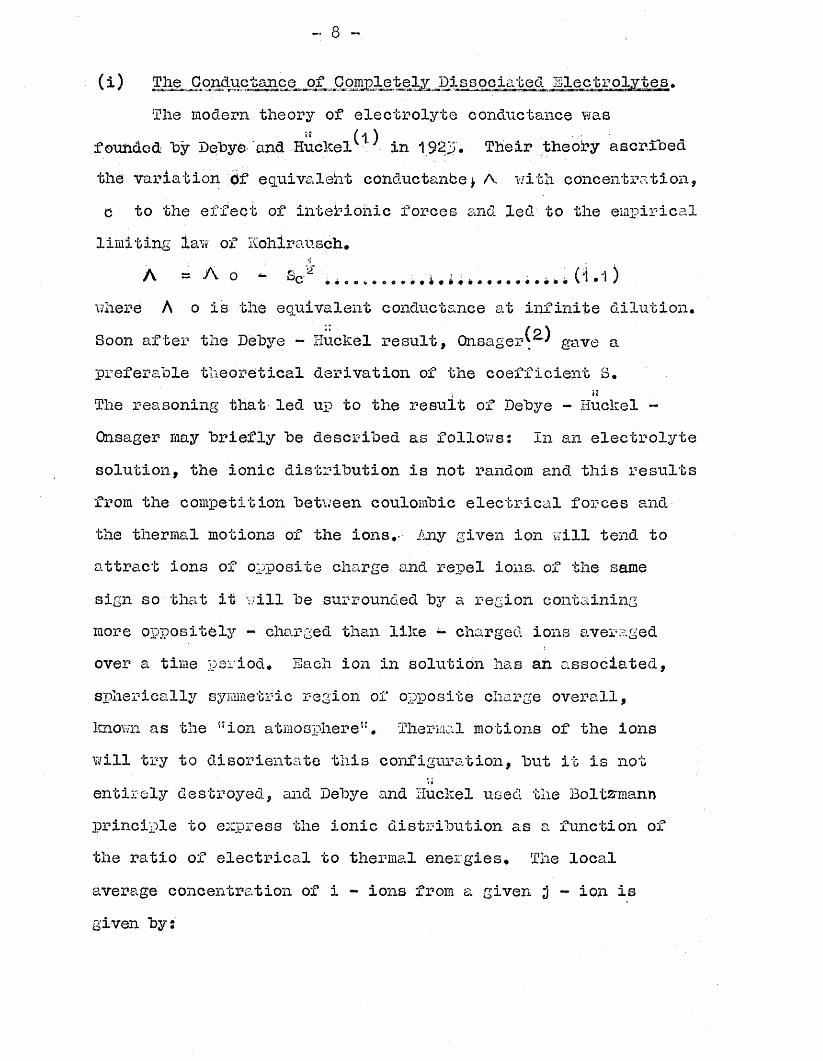
( i ) The, Conductanc e_,of,. CompletelxJD_j-s s oc ia t ed. ifThe modern theory of electrolyte conductance was

“ (1 )founded "by Debye and Huckel ' in 1923. Their theory ascr.ihed the variation df equivalent conductance* A. with concentration, c to the effect of intefriohic forces and led to the empirical limiting law of Sohlrausch.

A - A o *■ Sc 2 . w i. i. i i. i (‘S • )where A o is the equivalent conductance at infinite dilution. Soon after the Debye - Huckel result, Onsager^^ gave a preferable theoretical derivation of the coefficient S.

t * •The reasoning that led up to the result of Debye - Huckel - Onsager may briefly be described as follows: In an-electrolytesolution, the ionic distribution is not random and this results from the competition between coulombic electrical forces and the thermal motions of the ions.- Any given ion will tend to attract ions of opposite charge and repel ions, of the same sign so that it v.dll be surrounded by a region containing more oppositely - charged than like - charged ions averaged over a time period. Each ion in solution has an associated, spherically symmetric region of opposite charge overall, known as the ”ion atmosphere”. Thermal motions of the ions will try to disorientate this configuration, but it is not

i»

entirely destroyed, and Debye and Huckel used the Boltzmann principle to express the ionic distribution as a function of the ratio of electrical to thermal energies. The local average concentration of i - ions from a given j - ion is given by:

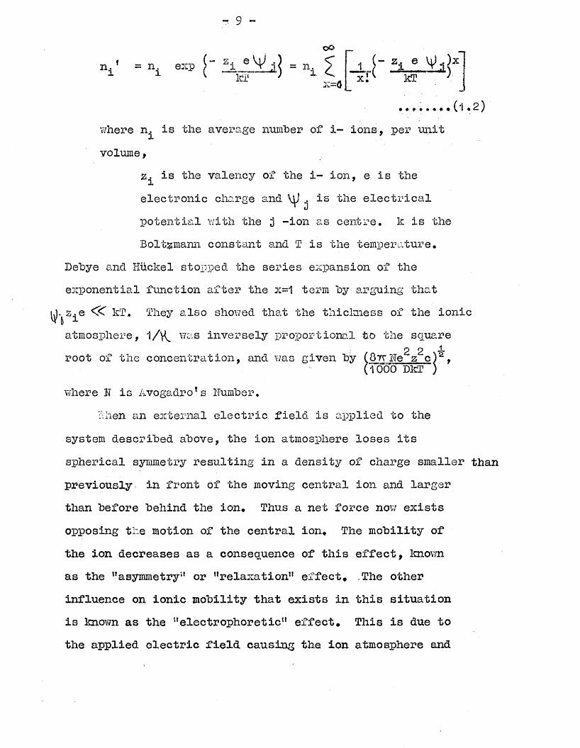
where ru is the average number of i~ ions, per unit volume#

z is the valency of the i- ion, e is theelectronic charge and \j is the electricalpotential with the 3 -ion as centre, k is theBoltzmann constant and T is the temperature.

Debye and Huckel stopped the series expansion of theexponential function after the x=1 term hy arguing that. Zje kT, They also showed that the thickness of the ionic b 1atmosphere, 1/V was inversely proportional bo the square

2 2 ~root of the concentration, and was given by (QrrHe z c}2,(1000 DkT )

where N is Avogadro’s Humber.when an external electric field is applied to the

system described above, the ion atmosphere loses its spherical symmetry resulting in a density of charge smaller than previously in front of the moving central ion and larger than before behind the ion. Thus a net force now exists opposing the motion of the central ion* The mobility of the ion decreases as a consequence of this effect, known as the ’’asymmetry” or ’’relaxation11 effect* .The other influence on ionic mobility that exists in this situation is known as the ’’electrophoretic” effect. This is due to the applied electric field causing the ion atmosphere and

- 10 -

its associated solvent molecules to move in the opposite direction to the motion of the solvated central ion. Thusthe central ion is effectively travelling in a medium whichis moving in the opposite direction. As would he expected, the electrophoretic effect is a function of the viscosity of the medium, , Finally, the motion of the ion %s opposed hy the frictional resistance, f, of the medium, described as a first approximation hy Stokes law:

f = 6 ts \rv ..... 0*3)where r is the radius of the ion and v is its velocity.

The above reasoning led to the Debye - Huckel *7

Onsager limiting equation for electrolyte condvictance:A = A Q - (S1 A Q + S2) ci ........ W . . (1.10

A 0 is the relaxation term and is the electrophoretic term. The ions are here represented as point charges.This eq.uati on may be regarded as a first approximation to

jlan equation describing a plot of A against d2. In the

f-r\ JLnomenclature of Fuoss'^ , a A/c 2 plot is called a phoreogram and so in practical terms, equation (1.4 ) represents the tangent to the phoreogram at o=0« In practice it v as found that the phoreograms of most uni-univalent salts approached the limiting law from above due to the non-zero size of the ions.

Other workers have attempted to extend and improve the Debye - Htickel treatment in order to produce conductance equations that represent more closely the phoreograms of strong electrolytes. One of the first attempts at improving

- 11 -

the limiting law was made hy Palkenhagen, Leist and Kelbgik)

who considered the ions to possess finite size. Two ions could not approach nearer than the distance r=a, and hence there could never he any charge inside a sphere of radius a around a reference ion except that of the ion itself. Instead of the Boltzmann distribution, a distribution‘function was used which allowed that not more than one ion could occupy the same site . The equation was formulated as :

and will he considered, in more detail in the high-frequency conductance section.

also made allowance for the distance of closest approach ofthe ions, and a appears in the eguation as the dimensionless

(Y )variable y (y=K a). The equation may be formulated as'

(1-5)

(6)A conductance equation produced by Pitts' 7 in 1953

1

(l+y)(2 2+y)JL2

with H = z2e2 H./3DkTc2 G = DkTHIH 09/r r r \C 21

( 8 C T z c c )2 (1OOODkT )

A = Ii(22-1 ) E = 3H2

D is the dielectric constant of the solvent and N isAvogadrofs number. and T are functions of y defined by Pitts

A series of conductance equations has "been produced by Puoss and others, resulting from revisions of the theory* The first equation, produced in 19 5 7^*'^, was in the form of a series in c :

AA ss Aq - Sc2 + Seine + Jc + ... ♦*.*•(1*7)The coefficient S is made up of two parts :

S = E1 A 0 - Ea (1 .8 )

and J is a function of a* No terms in higher powers of cwere evaluated and the first three terms of the Boltzmanndistribution (1.2) were used. Part of a term wasevaluated by Puoss and Berns^^ in a later equation :

A = A Q - Sc*' + Seine + J.c - J2c3//2... ( 1 . 9 )

In assembling the two equations (1.7) and (1.9)> a smalladditional term was included that has not been discussed

(1 1)above, resulting from inter ionic collisions' . Anion-cation attraction favours the possibility of additionalcollisions over the expected number for uncharged soluteparticles. When the asymmetry of the ion atmosphere isconsidered, the central ion will be struck more often byions of opposite charge from behind it than from in front.This will result in a slight additional component of velocityin the direction of travel. It is known as the “osmoticeffect;: and appears as a small term in the c coefficient.The complete Boltzmann distribution was retained in the 1965

( < 2 )equation of Fuoss, Qnsager and Skinner' , which also included an ion association term :

-- 2 A = A - S(coC) + Ecotf.n(c<*) + Jc<x — K-cocf A(1.1 0)

where is the association constant for the formation ofion pairs, and<*is the degree of dissociation*

A careful analysis of the differences between the Pittsand Fuoss theoretical models has been made by Pitts, Taborand Daly^^. rfTU''

(13) ,HsiaThe o'" *" terms were completed by Fuoss and

in 1967 to yield an equation of the form :A = ( A 0-AAe)(l +iOC/X )/(1+3J0/2 )A A is the electrophoretic term, e 7

(1.11 )

AX/X represents the relaxation and osmotic effects and 0 is the volume fraction of one species of ions, tp

take into account the effect of cations and aniojis moving around one another in their migrations.

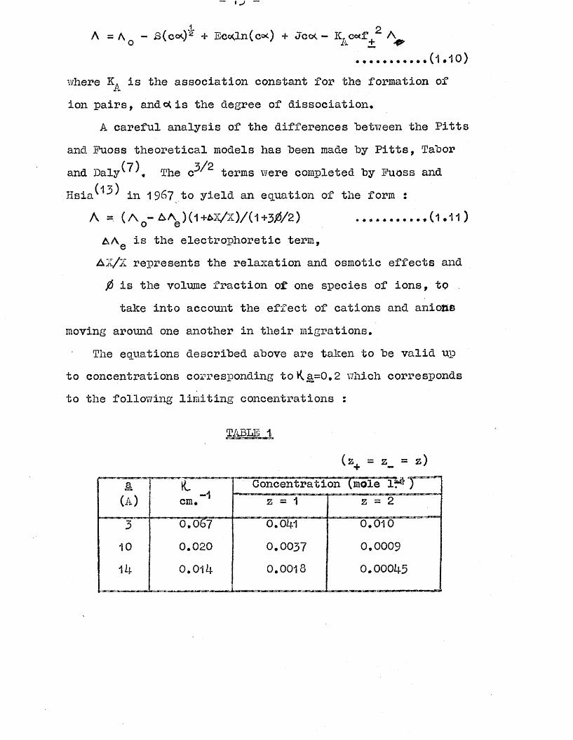
The equations described above are taken to be valid up to concentrations corresponding toKa=0,2 which corresponds to the following limiting concentrations :

TABLE 1

(z+ = z. = z)a Concentration (mole 1**0(A) cm."* z = 1 z = 23 o.oS7 O .041 0.01010 0 .0 2 0 0.0037 0.000914 0 .0 1 4 0.0018 0.00043

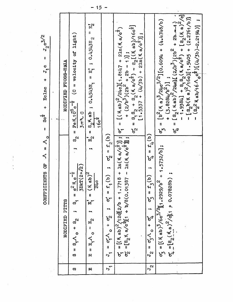
The equations of Pitts and of Fuosa-Hsia have been putinto the series form (1*9) "by Fernandez - Prini and P r u e ^ ^ ^ )who expanded the equations in pov/ers of c and neglected terms

■3/2ahove c . In the present work these expanded equationswill "be referred to as the "modified” forms of the completeequations and the expressions for their 8 , E, andcoefficients are shown overleaf, where b = ()z + 'I e )/ (a DkT)* In hoth equations the expressions for S and E arethe same* However, the functional forms of and arequite different for the modified equations of Pitts and ofFuoss - Hsia* For a given electrolyte-solvent system, Jand Jg are functions of a and A 0 ancl- are quite independentof concentration. The advantage of this method of seriesexpansion of the complete equations enables a term-by-termcomparison to be made between the Pitts and Fuoss - Hsia.equations. However, some differences may be expected betweenthe complete and modified forms due to neglect of terms above •3/2c ' in the modified equations. The differences between the

Pitts and Fuoss - Hsia equations are strongly reflected in the evaluation of the J coefficients. This may be illustrated by calculation of J and for the two modified equations for two model electrolytes in water at 2$°C. The two modelsare: 1 ) Uni-univalent (i :1 ) electrolyte with A = 130

-1 2 - 1 oohm cm. mole and a = 3*05 a, and2 ) Bi-bivalent (2 :2) electrolyte with A = 1 3 3 .0 7

—1 2 —1 0ohm cm* equiv. and a = 1^.32 A. The values of

- 15 -

CM

OCM

OhT

o£HOft

T-jjVIOCO

<II

eCO

ftHOH

o

i rrnr"N

OX ••k

•■CMft r-— i <^>CM r r ^ </—\ T"■Jcv CO J ©

II Ho* O p B . vO _©•<” s o MO Is- J "sd Is- ON+» CM X ■*— f— 1 -©• & CM T"JCS © X /■X • CM CM • CMto f t sHw -ct CO CM ••H P o + u—J ->—* CMiH i t v_/ © X 1<H

iA Pi j © + CM + +- it rH *« zsz P P

o • CM 1" "■> '—^ zd -©■ CM m fAO \— > v_' CTv ■—Mci o x

<4 + V CM Cl O O*

p *m

+3 • #v CO rH MO fA \•H r^- 1 CM • • W JO •» *-* -z t 1 o V” r-N

i O ft V p + U—J CM * Wsai-Hcsl_c0 H CO CM r~N r—l '—(■ —' •—V OCO © II • Hoi '—N CM • •» t— a CVl O Oo > V * O P X rH CO MO <p

IIV 1_» X IA «— 1 q -r-

^ CO_T-ft f t I— » CM © X O X MO

tr \ O P -=t J-CM CM CMP O i t -Pt CM -3? CM P X +

XCM\

f t fA CM v -/ X © pM i t X /—V CM + tA P * ^ f—v ©f t • CM A CO co P 4 s iH t-Jm O r~>

<Is- © CM © CO v—* X

0 1 P + A © J K> • * ON

P CMo o • «s © CM (A rs? CM CMa CO•o o p

CM IA CO • CM

IA ^ • ^ CM t-

00y Ml

COV -/

T“ ©Hw

o+ T~ P co

<__ i CO w J + U-Jt 1 1 1© CM MO II II II IIft to CO T-

II II V t w -fe ^ M *—\ /—sCM - CM P, *«s • e» P

CO f tCM

<HC = J -^

Hoi HwH t

• *

r~N

• s

••kII

V

o

>■s!s -/

H

II

V *

• •v

CMlAIs-lA

••r—

t-Km1

+CM

CM + 1+

O V_r P P 00 Is- Pzd © o S -/ T“ 00 CM p

Z iiT” r - a A P oo

CM p CM u r - T~ <H X CM© « o ON CO

IIIt T“ • II CM r -

II o ON o03 t — ** -T" V

+CO I P

CM•

»oEHEH

CO ft< P T~i

+*H CM •«v (X T 'f t V-gE# •5*

V

XfA

■r

pf t CM CM V "

CM_V

T“ OVO \

H 00 f t X H ^ ’ X CMf t + CM o + fA ^M + I <—N X ©P o P © o P A

-s ' J *v -r *

CMCO

OS O

<;T—o

< T*<;V

©S-«' CM

00

* <\P

©CO ft l—li_1 u—» u—JII (I

ii II 11 II II 11 \00 ft hT V CMh> \T >5*

* r CMCO ft h> 1*3

J, and J0 obtained are shown in Table 2 , from which It can 1 2 ’be seen that there are significant differences in and for the two modified equations, especially in the Jg terms. The value of (Pitts) is considerably larger than (Fuoss-Iisia) for both the 1:1 and 2:2 models.

Table 2

Coefficient ± • JL JlQdel p (Values x 10~ )

2:2 Model (Values x 10 )

J. ( Pitts (Fuoss-Hsia

2.41 6 1 .969

2.03941.3303

J ( Pitts (Fuoss-Hsia

3.6491.740

13.80329 .230 8

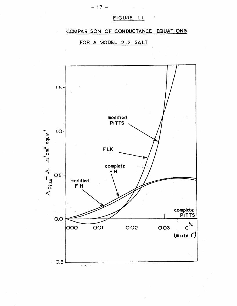
A general comparison was made between the equations used in this work in terms of their numerical predictions for a 2:2 electrolyte. The model electrolyte was chosen as above and complete dissociation was assumed. Then the values of /\ calculated from these equations v/ere compared for various values of c by plotting ( A Pitts - A ) against -- (1 6)c2. Similar comparisons have been made by Prue et al. *A Pitts is the conductance calculated by the complete Pitts equation, which is represented on the graph as the abscissa. The graph is illustrated in Figure 1.1. The numerical differences between the complete and modified forms of the Fuoss-Hsia equation are very small over the concentration range studied (0 - 0.0016 M), whereas differences between the complete and modified forms of the Pitts equation are

- 17 -

FIGURE I.)

COMPARISON OF CONDUCTANCE EQUATIONS

FOR A MODEL 2 :2 SALT

modifiedPITTS

.0-

c r

FLK

completeFH

0 .5 -modified

completePITTS

0.0

0.00 0.01 0.02 0 .0 3

-0 .5

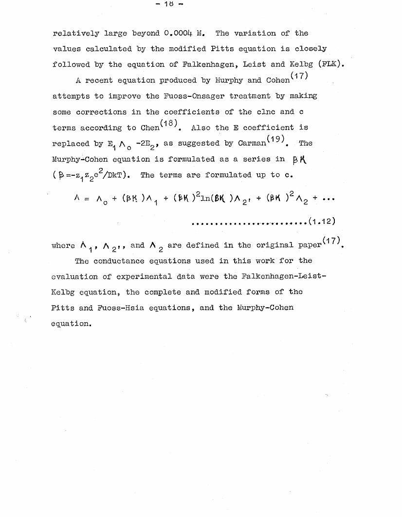
relatively large 'beyond 0.0004 M. The variation of thevalues calculated by the modified Pitts equation is closelyfollowed by the equation of Falkenhagen, Leist and Kelbg (FLK)

(i 7 )A recent equation produced by Murphy and Cohenattempts to improve the Fuoss-Onsager treatment by makingsome corrections in the coefficients of the clnc and cterms according to Chen^^. Also the E coefficient is

(1 9)replaced by A 0 ~2E2 , as ^ Carmanv TheMurphy-Cohen equation is formulated as a series in

p(p>=-z^z2e /pkT). The terms are formulated up to c.

A = A 0 + O K ) A 1 + (£K )2l n O K ) A 2( + O K )2 A 2 + •••

(1.1 2)(17)where A , A 2 «> an< A 2 are defined in the original paperx

The conductance equations used in this work for the evaluation of experimental data were the Falkenhagen-Leist- Kelbg equation5 the complete and modified forms of the Pitts and Fuoss-Hsia equations, and the Murphy-Cohen equation.

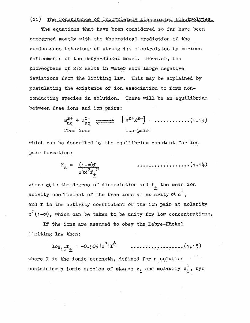
(ii) The Conductance of incompletely Dissociated Electrolytes, The equations that have "been considered so far have heen

concerned mostly with the theoretical prediction of the conductance "behaviour of strong 1:1 electrolytes hy various refinements of the Debye-Htickel model. Hov/ever, the phoreograms of 2 :2 salts in water show large negative deviations from the limiting law. This may he explained hy postulating the existence of ion association to form non­conducting species in solution. There --will he an equilibrium between free ions and ion pairs:

+ 0 +Xzi ...........(1.13)free ions ion-pair

which can he described hy the equilibrium constant for ion pair formation:

.................... . . . . . . . . . . . ( i . i i + )

c a f

where o^is the degree of dissociation and f_, the mean ion acivity coefficient of the free ions at molarity c< c ’, and f is the activity coefficient of the ion pair at molarity c‘(l-o<), which can he taken to he unity for low concentrations,

If the ions are assumed to obey the Debye-Htickel limiting lav/ then:

log10f+ = -0.509 |z2Ii ........,..........(1.15)

where I is the ionic strength, defined for. a solution containing n ionic species of charge z. and molarity c , by:

J. •*-

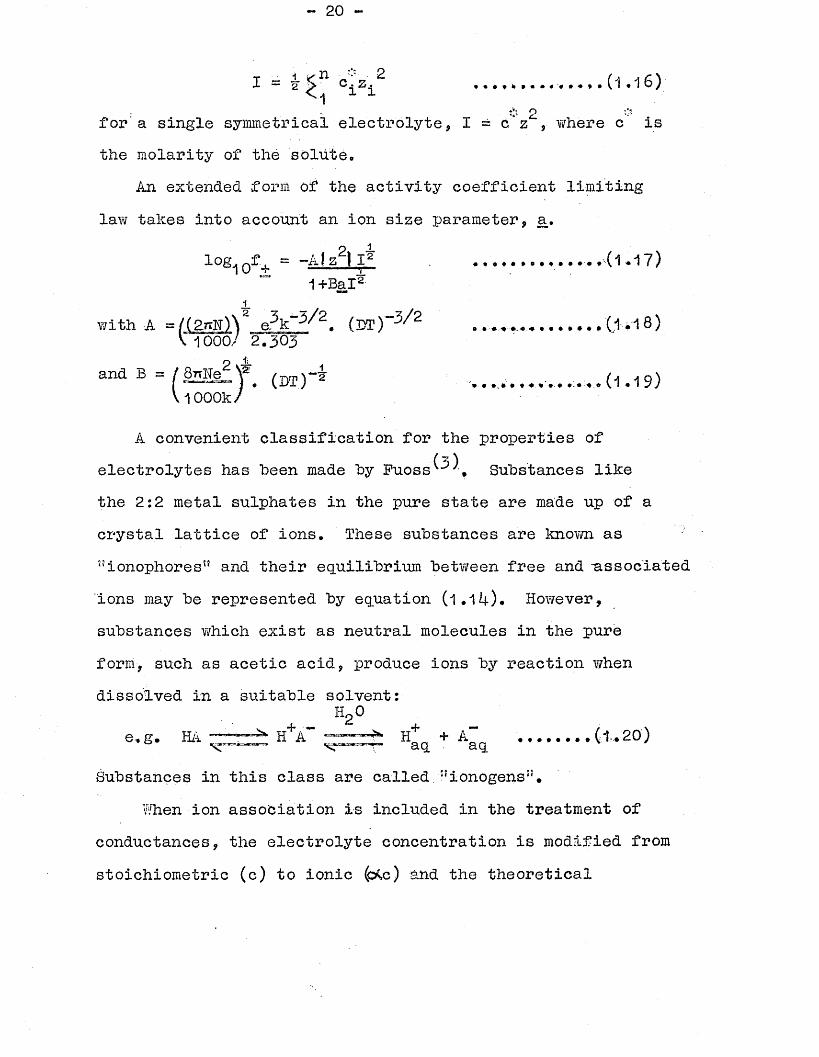
- 20 -

I = ¥ ^ n Cizi2 (1 .1 6);: b 2'for a single symmetrical electrolyte, I = c z , where c is

the molarity of the solute.An extended form Of the activity coefficient limiting

law takes into account an ion size parameter, a.

log1of + = “A is fL f l ................... . . . . . ( 1 - 1 7 )" l+Bal^

Xwith A = /(2nN) \ 2 e.3k~3/W (Kr) -3 //2 ............(1.18 )

V 1000/ 2 .303

and B = /§nm£W (m)~i ...>..........(1.19)\ 1000k/

A convenient classification for the properties of(*)electrolytes has heen made hy Fuoss % Substances like

the 2 : 2 metal sulphates in the pure state are made up of a crystal lattice of ions. These substances are known as ”ionophores!} and their equilibrium between free and "associated ions may be represented by equation (1.1/+)* However, substances which exist as neutral molecules in the pure form, such as acetic acid, produce ions by reaction when dissolved in a suitable solvent:

h2oe.g. HA ■ ■ ' 1 s H+A~ -----*■ H* + A~ ...... ( 1 . 2 0 )■\ v ' ' ‘ 1. aq aq

Substances in this class are called :jionogens5?.When ion association is included in the treatment of

conductances, the electrolyte concentration is modified from stoichiometric (c) to ionic (c*»c) and the theoretical

- 21 -

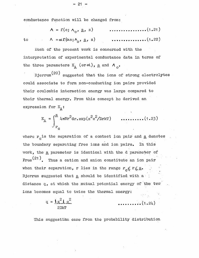
conductance function will Be changed from:

A = f(c; A0, a., z) ................(l.2 1)

to A = e*f(c*c;Ao, a, z) .....

Much of the present work is concerned with theinterpretation of experimental conductance data in terms ofthe three parameters K. (orc<), a and A .a o

B;jerrum^^ suggested that the ions of strong electrolytescould associate to form non-conducting ion pairs providedtheir coulomhic interaction energy was large compared totheir thermal energy. From this concept he derived anexpression for K :

V

= f~ .TtMr dr.exp(z2e2/DrkT) ••••••••••(1.23)

r o

where 3?cis the separation of a contact ion pair and a denotesthe Boundary separating free ions and ion pairs. In thiswork, the a parameter is identical with the d parameter of

(21 )Pruev ', Thus a cation and anion constitute an ion pair when their separation, r lies in the range rc^ /Bjerrum suggested that a should he identified with a distance q., at which the mutual potential energy of the two' ions Becomes equal to twice the thermal energy:

2 21 = i z J L e _ .........

2DkT

This suggestion came from the proBaBility distribution

of oppositely charged ions at a given distance r from a central ion, . The distribution curve showed a minimum at r = q, For aqueous solutions at 23°C, q = 3.57 z2 2„Thus for uni-univalent electrolytes the critical distance is 3*37 2 , and the value is 1 ^ *3 2 2 for bi-bivalent electrolytes,.

(22)An alternative approach due to Denison and Ramsayx 7 (2 )and Fuossv ^ 7 suggested that two ions should constitute an

ion pair only when they were in contact, with no intervening molecules betv/een them. The expression for in this case is:

KA = ^ . exp( z2e2/DrcKT ) (1.25)3

(2i )with the assumption that a = kr /3 . In both of the** cabove models the solvent is taken to be a continuous, structureless medium, characterised by a bulk viscosity and dielectric constant.

The equilibrium between free ions and ion*pairs may be further refined by the additional concept of various ion- pair states. From an analysis of the ultrasonic absorption data for 2 :2 metal sulphates, Eigen'2 proposed that the associated ions could have one or more interposing solvent molecules between the ions (outer-spbe/re ion-pairs) or they could exist with the ions in contact (inner-spheve, ion-pairs). Thus the free ion - ion-pair equilibrium would consist of the following stages:

- 23 ^

26)The upper limit,. a in this case is given "by the sum of

the ionic radii plus the diameters of two solvent molecules. - Neithei* of the ioii-pair states contributes to electrical conductancei Each, ion-pair model described above implies a different value for a. For 2:2 salts, the Bjerrum q distance is 14.32 S, the Eigen value is approximately 10 2. and the centre-to-centre distance of a contact ion-pair is of the order of 4 &«. Thus for a particular 2:2 electrolyte under consideration there is a wide range of values for the choice of the a parameter. In this context, it is important to realise how the choice of the a parameter will affect conductance values calculated from a given theoretical equation.

In the present work the effect of the variation of a in a number of theoretical equations has been investigated. Equivalent conductances were calculated using the complete and modified forms of the Pitts and Fuoss-Hsia equations, and the Falkenhagen-Lelst-'Kelbg equation* for. a values in the range 2-14 S. with- A = 1 33.0? ohm”**1 cm.2equiv..The conductances were calculated for two concentrations :

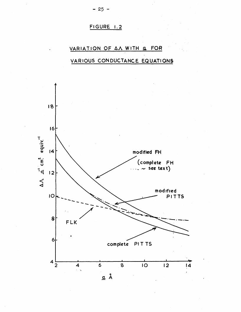
10 “ M (giving A 0 .0001 val'aes) and M (giving A 0#00ivalues). A convenient way to represent the results is then to plot A A (= Aq 0001 - A q 00i ) against a. The quantityAA is, to a first approximation, proportional to the slope

— *-3of the A/c 2 plot in the concentration range 0 - 10 ^ M,and so the variation of A A with a will indicate the effect of a on the slope of this plot. The results are illustrated in Figure 1.2. In general, an increase in a will decrease AA and so increase A values for a given A q at a particular concentration. The results for the complete Fuoss-Hsia equation were' so close to those of the modified form that they have been omitted. The A A values for the complete and modified Pitts equations are very close up to a = 4.8 for a values greater than this, the modified Pitts gives smaller A values than the complete form of the equation (c.f. Figure 1.1)# The A values calculated hy the Fallrenhagen Leist-S£elbg equation are affected much less hy a change in a than any of the othei7 equations and the values become very close to those of the modified Pitts equation for a greater than about 10 S.

AA

n cm

. eq

uiv.

- 25 -

FIGURE 1.2

VARIATION OF A A WITH a FOR

VARIOUS CONDUCTANCE EQUATIONS

I

modified FH

(complete FH .... ^ see text)

modified - P I T T S

F LK

complete P I T T S

e

PART I SECTION 2

HIGH-FREQUENCY CONDUCTANCE

- 27 -

(i) The Theory of High-Frequency Conductance.* * i.Ht r^meB3*£a*ata*s&m/ i0 iffK mm>'. * ■■ ■ IT Jlj grdW'i i «. j pii »m mdMuJlitMPi wr Mi h * I ■ i • ■ — ■». WV W » ■

It was noted in the last section that when ions in an electrolyte solution are subjected to an electric field, the ionic atmosphere takes up an asymmetric distribution relative to its reference ion. If the disturbing field is then removed, this asymmetry will disappear in a finite time, known as the relaxation time of the atmosphere, 0; if this relaxation time did not exist, there would be no electrical force of relaxation* If an alternating electric field is applied across the solution, each ion executes an oscillatory motion of the same frequency as that of the field. For low frequencies of the applied field, this situation produces an asymmetric charge distribution within each half-cycle, corresponding to the stationary or direct-current case. However, v/hen the frequency of the field is sufficiently high so that the period of oscillation of the reference ion is comparable to the ion atmosphere relaxation time, there will be insufficient time for the asymmetric charge distribution to be developed completely. Thus the relaxation force can be expected to decrease with increasing frequency of the applied field, resulting in increased ionic mobility and therefore increased conductance. Thus an increase or “dispersion5' of conductance can be expected for electrolytes at radial

/ o c frequencies of the order of 1/9, Debye and Falkenhagen^ first considered the importance of the ion atmosphere relaxation time, and they derived an expression for 0 for

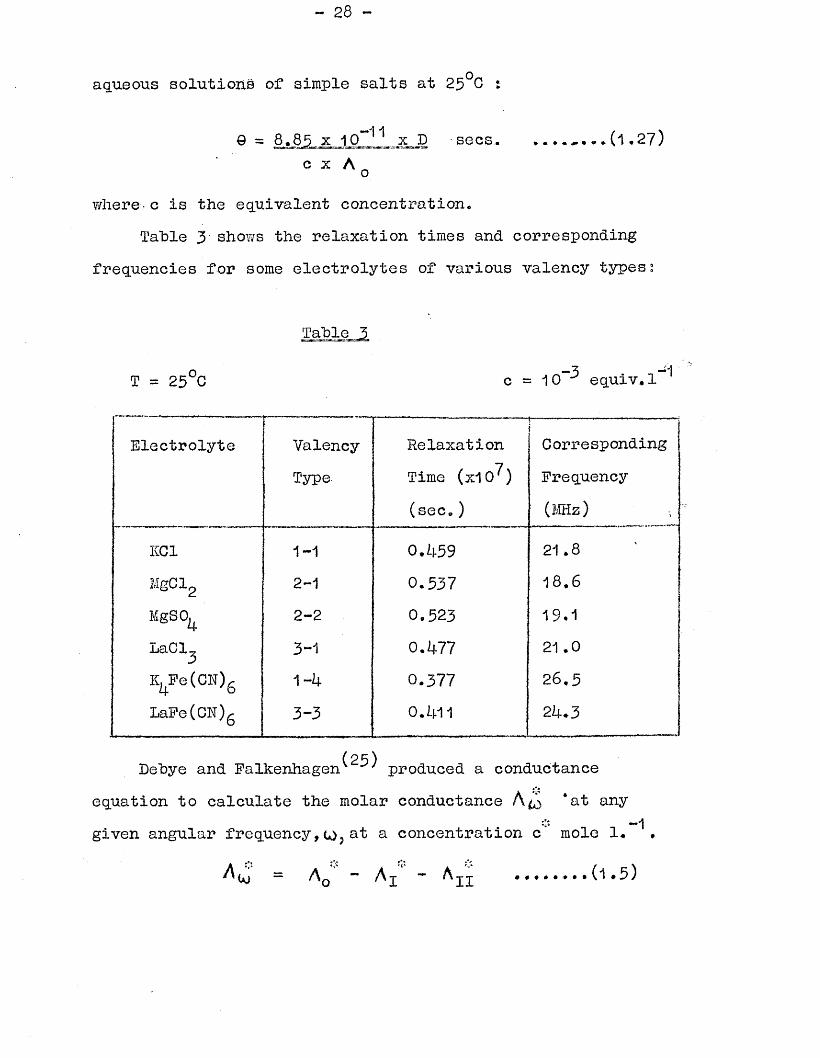
aqueous solutions of simple salts at 25°C :

Q - 8.85 x 10~11 x D secs...... ^ . (1.27)c X A o

where-■ c is the equivalent concentration,,Table 3 shows the relaxation times and corresponding

frequencies for some electrolytes of various valency types;

Table 3

T = 25°C c = 10-3 equiv. 1

Electrolyte ValencyType

Relaxation Time (x10 ) (sec,)

i-- ---- --- -—..—1CorrespondingFrequency(MHz)

KOI 1-1 0.459 21.8MgCl2 2-1 0.537 18.6MgSO^ 2-2 0.523 19.1LaCl-, 3H 0.477 21 .0K4Pe(CN)6 1-4 0.377 26.5LaPe(CN)g 3-3 0.411 21+.3

(25)Debye and Falkenhagen J produced a conductance equation to calculate the molar conductance 4at any

-1given angular frequency, u>? at a concentration c mole 1. •

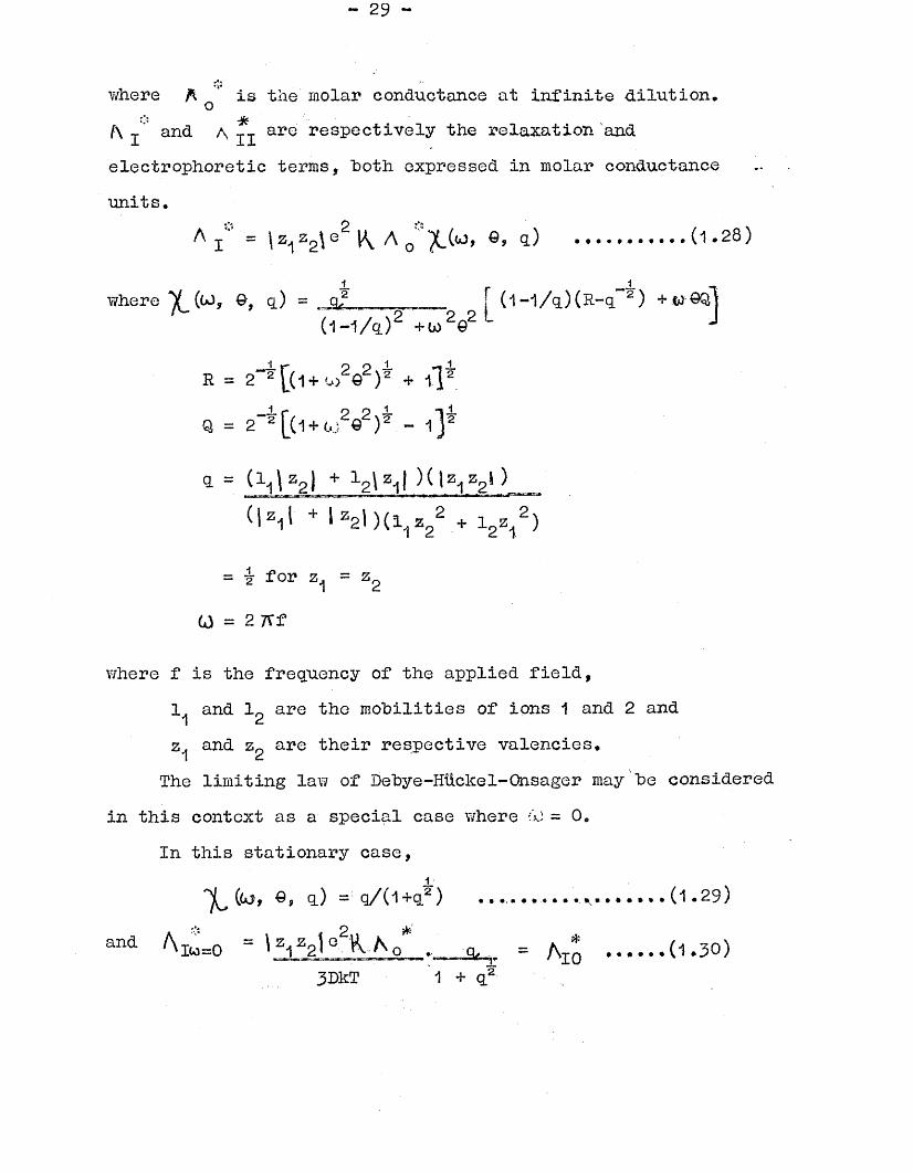
where ft ‘ is the molar conductance at infinite dilution,o* *[\ j and A arG respectively the relaxation and

electrophoretic terms, both expressed in molar conductance units.

A I° = 1Z1Z2^ 2 ^ A o:!7 (<0* 9’ .(1.2 8)

i r -- -t:where ( ^ 5 0 , a) - a.2 | (l-l/q)(R-q 2) + &)3Q|(1-1/q) 2 + w 2e2 ' -*

e = 2"^[(i+ W 2e2) + \\*

Q = 2- ? [(-i + to2e2 )1' - -i]*

a = (i.i\z2) + 1P\z-il )(lzizP>)(|^l + I z2l Hi, z22 + l ^ 2)

= i for Zjj = z2

0) = 2 7Vf

where f is the frequency of the applied field,1, and 10 are the mobilities of ions 1 and 2 and 1 2Zj and z2 are their respective valencies.

The limiting la?/ of Debye-Hiickel-Gnsager may be considered in this context as a special case v/here 6J = 0.

In this stationary case,

^ ((O, e, q) = q/(l+q2) ..(1.29)

and ^lu=0 = lz1z2^°2^ A o . Q, = A zq ..... (1.30)3DET 1 + aj

- 30 -

Only the relaxation term is frequency-dependent;the electrophoretic term will he the same for thestationary and high-freguency cases (the term high-frequency means any frequency at which the dispersionof conductance "becomes apparent - in practice this is

5 \greater than about 10* Hz.).

^11 = ^ z1> * l z2t K, ...........(1.31)6n r. n

where F is the Faraday constant and is the viscosity of the solvent*

The percentage increase in conductance, or the “dispersion” of conductance, is given by:

& % = l\i*> - Au)-p x 100% .....(1.32)^ ty =0

The Debye-Falkenhagen theory considered the ions only as point charges, and the treatment was further refined in 1952 by Falkenhagen, Leist and Kelbg^^ who accounted for the effect of finite ionic size, as an a parameter, on high-frequency conductance. The Falkenhagen-Leist-Kelbg equation is formulated as (1*5) but with modified relaxation and electrophoretic terms:

- 31 -

a ; i = W 2 » ° 2K a 11 21 n ^ o, a.3DkT ( ( l - a )2+g26j 2e2 ) ( K a(l + K a))

exp(fta(l-q.z)R)[(l-q.)cos(\ aQ<i2) +

quQsind^ aQq2) -(l-q.)| ,.....(1.33)

a

If (1.33) and (1,34) are evaluated with a = 0, the simpler Debye-Falkenhagen terms (1.28) and (1.31) will he obtained.

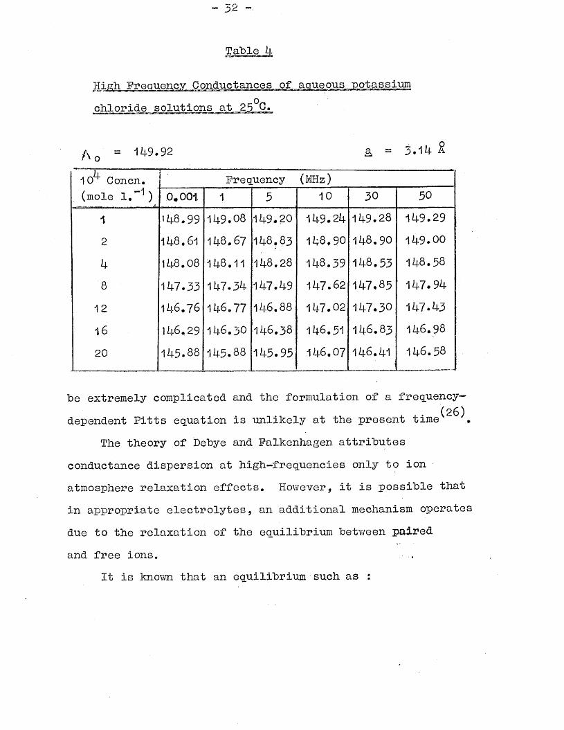
'The data of table k illustrates the effect of a high- frequency field on conductance. Equivalent conductances, calculated by the Falkenhagen-Leist-Kelbg equation are given for potassium chloride solutions for a number offrequencies and concentrations using a A value of li+9.92

—1 2 —1 P (9 0)ohm cm. equiv. and an a parameter value of 3.14 A •The equation of Falkenhagen-Leist-Kelbg has been used

in the present work for the calculation of high-frequency conductance. It is one of the very few conductance equations which treat the (w =0) condition as a special case of alternating field conductance. The possibility of extending other stationary field conductance equations to frequency dependence seems remote: an extension of the Fuoss-Onsager treatment to alternating fields appears to

High Frequency Conductanceschloride solutions_at 25

A 0 = 92 a = 3.14 £

10 Concn. (mole 1. )

Frequency (MHz)0,001. 1 5 10 30 50

1 'AS- 99 149.08 149.20 149.24 149.28 149.292 148.61 148.67 148.83 148.90 148.90 149.00

4 148.08 148.11 148.28 148.39 148.53 14 8 .5 8

8 147.33 147.34 147.49 147.62 147.85 147.9412 146.76 146.77 14 6.88 147.02 147.30 147.4316 146,29 1 4 6 .3 0 146.38 146.51 146.83 146.9820 145.88 145.88 145.95 146.07 146.41 146.58

he extremely complicated and the formulation of a frequency­'s)dependent Pitts equation is unlikely at the present time

The theory of Debye and Falkenhagen attributes conductance dispersion at high-frequencies only to ion atmosphere relaxation effects. However, it is possible that in appropriate electrolytes, an additional mechanism operates due to the relaxation of the equilibrium between paired and free ions.

It is known that an equilibrium such as :

- 33 -

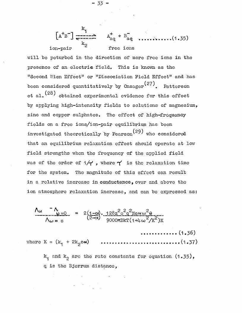
[aV ] ^--- ^ Aag + BIq. ...... ..... .(1.35)ion-pair free ions

will "be peturbed in the direction of more free ions in thepresence of an electrie field* This is known as. the"Second Wien Effect" or "Dissociation Field Effect" and has

(27)"been considered quantitatively by Onsager . Pattersonet al. obtained experimental evidence for this effectby applying high-intensity fields to solutions of magnesium,zinc and copper sulphates* The effect of high-frequencyfields on a free ions/ion-pair equilibrium has been

(29)investigated theoretically by Pearson J who considered that an equilibrium relaxation effect should operate at low field strengths when the frequency of the applied field was of the order of , where 'Y is the relaxation time for the system. The magnitude of this effect can result in a relative increase in conductance, over and above the ion atmosphere relaxation increase, and can be expressed as:

o 9000nDkT(l + i j . o j 2 / K 2 ) K

........... (1.36)where K = (k + 2kgC«t) .... ............... •*(1.37)

k and kg are the rate constants for equation (1.33), q is the Bjerrum distance,

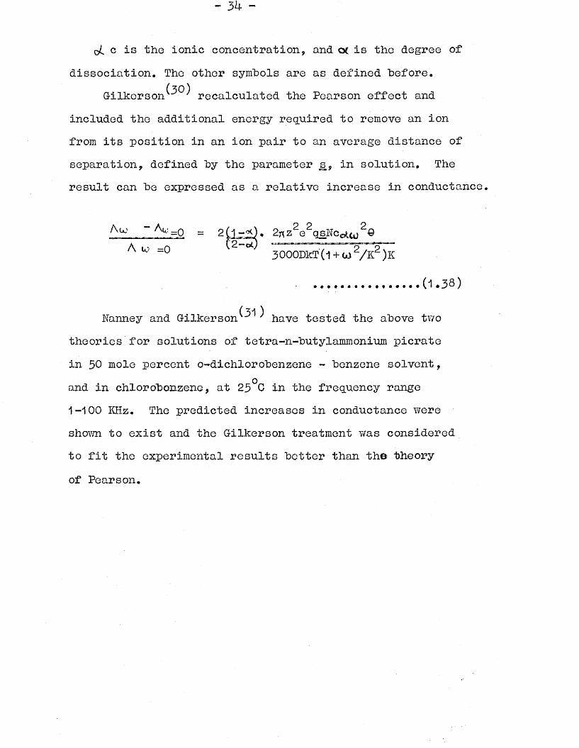
c is the ionic concentration, and at is the degree of dissociation. The other symbols are as defined before.

Gilkerson^^ recalculated the Pearson effect and included the additional energy required to remove an ion from its position in an ion pair to an average distance of separation, defined by the parameter s9 in solution. The result can be expressed as a relative increase in conductance,

2(1 -'*)♦ 2nz2e2qs,Ncotw «3000DKT (1 + W 2/K2 )K

(1.38)

( 31 )Nanney and G-ilkerson 7 have tested the above twotheories for solutions of tetra-n-butylammonium picratein 50 mole percent o-dichlorobenzene - benzene solvent,

oand in chlorobonzene, at 25 C in the frequency range 1-100 KHz. The predicted increases in conductance were' shorn to exist and the G-ilkerson treatment was considered to fit the experimental results better than the theory of Pearson.

The dependence of conductivity of an electrolyte solutionon the frequency of an applied field was first observed by

( 32 }Y/ien ' during the course of experiments on the variation ofconductance with field strength. The frequency effect was

(25) (33)treated theoretically by Debye and Falkenhagen , and Sackv y was the first to obtain quantitative results at sufficiently high radio-frequencies. The increases in conductance were found to be of the correct order of magnitude as predicted by theory.

The usual Y/heatstone bridge arrangement for the determination of conductanee cannot be used at radio-frequencies. As the frequency increases it becomes increasingly difficult to maintain the symmetry of the bridge system because the inductance of the connections and components of the bridge network will become increasingly important. Alternative measurement techniques have been devised to avoid this problem and the most important ones were devised by Sack^^ (resonance circuit), Zahn^^ (oscillatory current in electromagnetic field), Deubner^^ (valve oscillator), ?/ien^^ (resonance circuit) and Malsch^"^ (calorimetric method).

Owing to the very difficult nature of radio-frequency measurements, most authors restricted their investigations to one or two concentrations and often to one frequency.

/ 70 \,

Arnold and YYilliams^ ' made a systematic study of conductance dispersion for electrolytes of as many different valency

- 36 -

types as possible* The results showed that the dispersion of conductance increased with the valency product of the ions and with the frequency. The dependence of conductivity dispersion on the concentration, temperature, valency of ions and dielectric .constant has been • ©anaidtercd by FaIkeullagen^^ and Falkenhagen and williams

(25)The theory of Debye and Falkenhagen 7 predicted thatthe diele ctric constant of a solution at zero frequency wasa function of the solute concentration:

Dw = 0 - Dq = SD (..)* (1.39)where D , is the zero frequency, dielectric constant ofthe solution, D^ is the solvent dielectric constant and thecoefficient SD 1ms been evaluated for a number of electro-

(39)lytes . Further, the theory predicts a change m the dielectric constant of the solvent in a solution with the frequency of an alternating field. An increase in the angular frequency, w, decreases the ”solution” dielectric constant, Dy, which tends towards D^at very high-frequencies* This is illustrated in Table 5 where D*j has been calculated for magnesium sulphate solutions at several frequencies.

Under the conditions of concentration and frequency employed in this work, the dielectric constant changes have a negligible effect on the interpretation of conductances.The usual practice has been followed of assuming that the dielectric constant of the medium in which the ions are placed remains constant, independent of the ionic sti’ength of the solution.

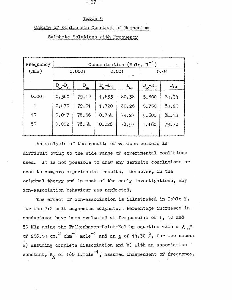
Change of Dielectric Constant _of Magnesium Sulphate Solutions with Frequency

Frequency Concentration (Mol□ . l“1)(MHz) 0

;.0001 0.001 0.01

D -Do D -D x w 0 Dto d -da1*3 00.001 0.580 79.12 1.835 80.38 5.800 84.341 0,470 79.01 1.720 80.26 5.750 84.2910 0.017 78.56 0.7 34 79.27 5.600 84.1450 0.002 78*514- 0.028 78.57 1.160 79.70

An analysis of the results of various workers isdifficult owing to the wide range of experimental conditionsused. It is not possible to draw any definite conclusions oreven to compare experimental results. Moreover, in theoriginal theory and in most of the early investigations, anyion-association behaviour was neglected.

The effect of ion-association is illustrated in Table 6•for the 2:2 salt magnesium sulphate. . Percentage increases inconductance have been evaluated at frequencies of 1 , 10 and50 MHz using the Palkenhagen-rLeist-Ker.bg equation with a Aof 266*1 If. cm.^ ohm~ mole and an a of 14.32 S, wo casesa) assuming complete dissociation and b) with an association

-1constant, of i 80 l.mole , assumed independent of frequencyA

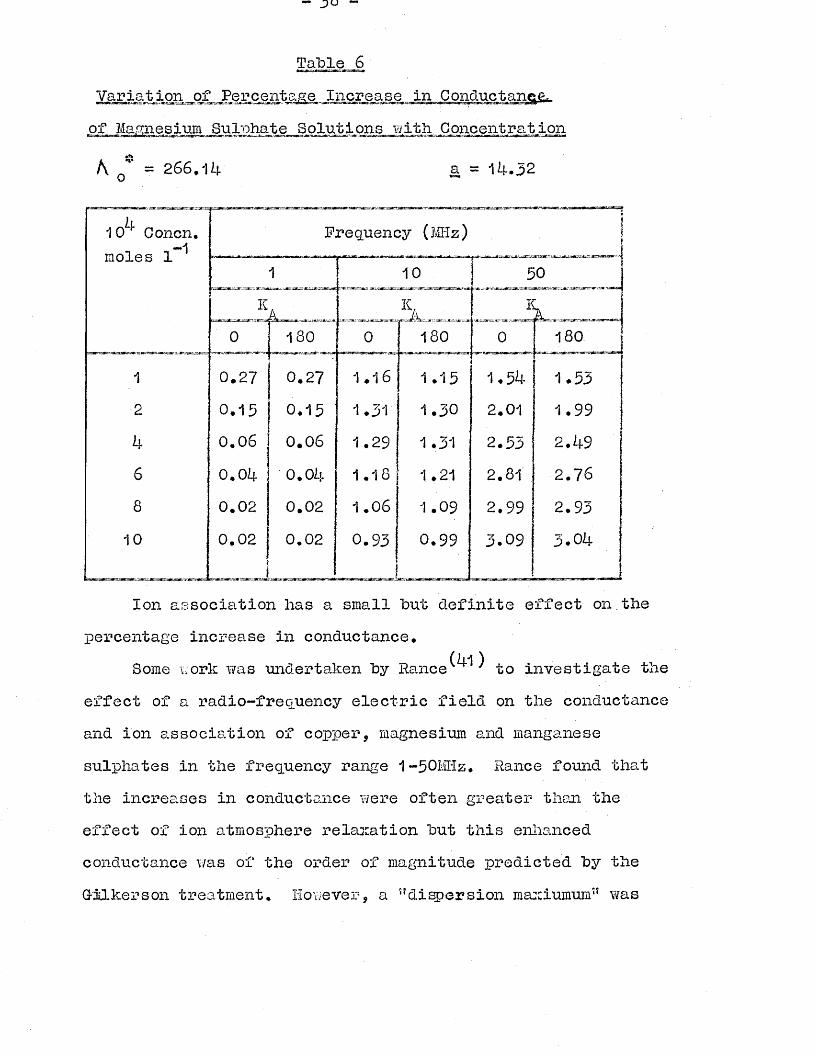
Table 6Variat.ion._of.JPer.ce_iTfcage Increase in Conductance^ of Magnesium Sulphate Solutions with Concentration

A, Qn* = 266.14 a = 14.32

Frequency (MHz)10 Concn -1moles 1

180180180

0.270.271.992.011.31

0.06 0.06 1.292.762.810.04

0.02 2.930.02 1 .09 2.990.02 0.93 0.990.02

Ion association lias a small but definite effect on.thepercentage increase in conductance.

Some work was undertaken by Ranee^ to investigate the effect of a radio-frequency electric field on the conductance and ion association of copper, magnesium and manganese sulphates in the frequency range 1-50MHz. Ranee found that the increases in conductance were often greater then the effect of ion atmosphere relaxation but this enhanced conductance was of the order of magnitude predicted by the G-ilkerson treatment. However, a ” dispersion maxiumuijfJ was

- 39 -

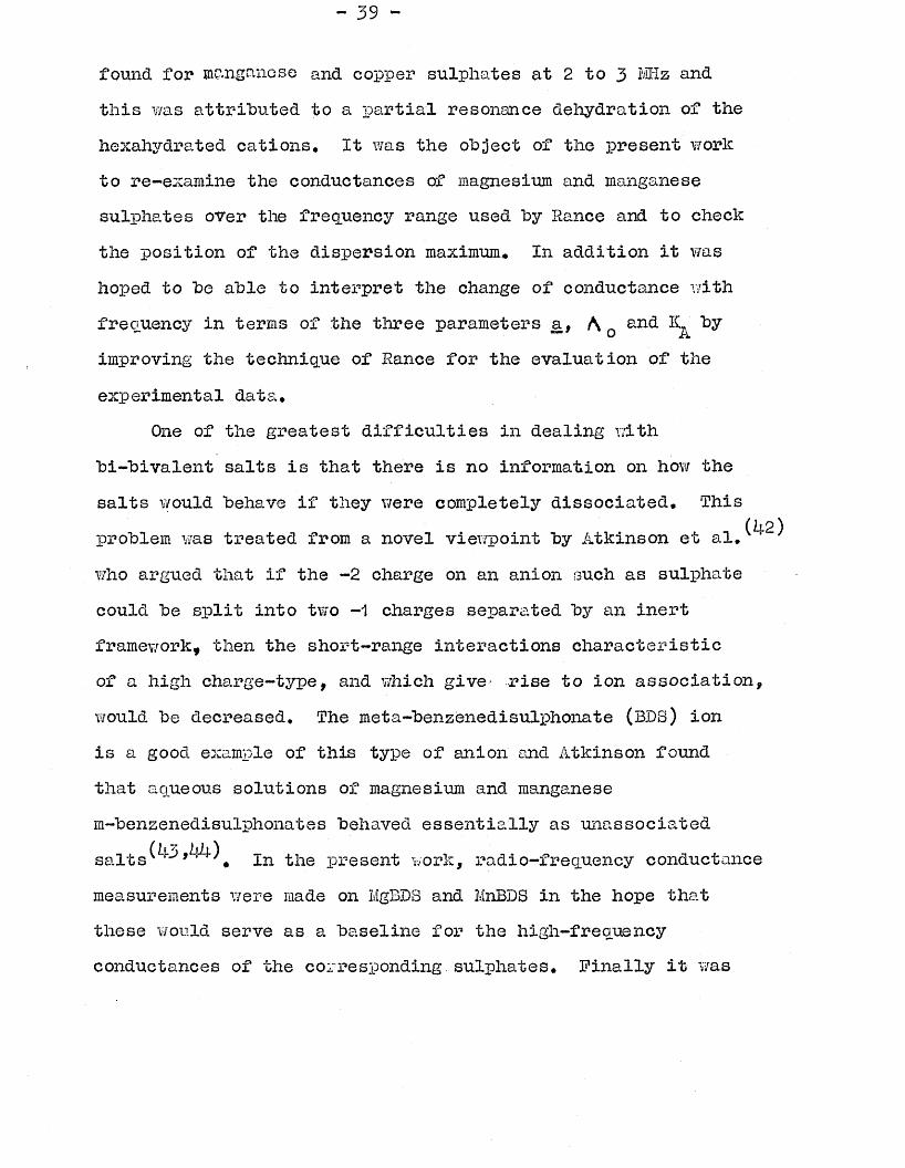
found for manganese and copper sulphates at 2 to 3 MHz. and this was attributed to a partial resonance dehydro-tion of the hexahydrated cations. It was the object of the present work to re-examine the conductances of magnesium and manganese sulphates over the frequency range used by Ranee and to check the position of the dispersion maximum.. In addition it was hoped to be able to interpret the change of conductance with frequency in terms of the three parameters a, A 0 an& ^ improving the technique of Ranee for the evaluation of the experimental data.

One of the greatest difficulties in dealing with bi-bivalent salts is that there is no information on how the salts would behave if they were completely dissociated. This

(1l2)problem was treated from a novel viewpoint by Atkinson et al. * who argued that if the -2 charge on an anion such as sulphate could be split into two -1 charges separated by an inert framework, then the short-range interactions characteristic of a high charge-type, and which give- rise to ion association, would be decreased. The meta-benzenedisulphonate (BDS) ion is a good example of this type of anion and Atkinson found that aqueous solutions of magnesium and manganese m-benzenedisulphonates behaved essentially as unassociated s a l t s I n the present work, radio-frequency conductance measurements v/ere made on MgBDS and MnBDS in the hope that these would serve as a baseline for the high-frequency conductances of the corresponding.sulphates. Finally it was

- 4 0

hoped to use the audio-frequency data of the sulphates and m^henzenedisulphonates to compare the complete and modified Pitts and Puoss-Hsia equations and the equations of Falkenhagen-Liest-Kelhg and Murphy-Cohen in terms of the three parameters \ Q, a, and

PART II SECTION 1 APPARATUS

~ 42 -

The conductance measurements that were made during the course of this work may he divided into two groups: audio­frequency (AF) measurements (made at IKKz) and those measurements made at radio-frequencies (KF). The AF measurements v/ere made using a Wheat stone bridge, and HF conductances were determined using two transformer ratio-arm bridges: one covering the range 0,1-5 MHz and the otherextending this range to 100 MHz.(i) Audio-frecmency apparatus

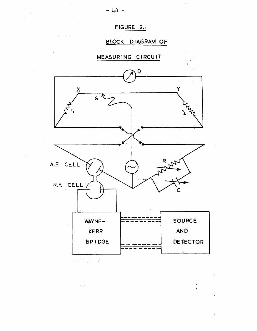
For the conductance measurements at 1 KHz, aconventional Wheatstone bridge was used, having a slide>wire modified for increased precision. This circuit isessentially the one proposed by Davies^*^ for conductancework. The circuit details are shown in Figure 2.1. Theslide wire, XY, of low temperature coefficient of resistance,was stretched over a metre rule. This arrangement togetherwith the sliding contact S v/as obtained as a slide wiredetector unit from Messrs. Griffin and George. Non-reactive100 ohm resistors, r, and r^, were connected to each end of1 2the v/ire. The wire had a resistance of 2 ohms so that the whole arrangement v/as equivalent to a 101 metre Y/ire, and each mm. of the wire had 1/101 ,000 of the resistance of the whole. The position of the balance point was read to 0.5 mm.

The non-reactive resistance R was a five-decade Sullivan box (type A.C. 1013) of total resistance 11,111 ohms in steps of 0.1, 1, 10, 100 and 1000 ohms. The capacitance

- 43 -

of the solution ■under investigation was balanced out with a general Radio decade capacitor G having a capacitance range of 1/jlF to 1 pF. The two components, R and G v/ere standardised by the National Physical Laboratory. The conductance cell v/as connected in the remaining arm of the bridge and the cell and R could be interchanged with respect to the bridge wire to give two positions of balance. These two positions v/ere not equivalent since the values of r and r were not identical and so the true balance position was determined from the arithmetic mean of two or more measurements.

The bridge source was a Farnell Instruments oscillator(type LFM2), The oscillator had a frequency range of

6(1-10 ) Hz but was usually used at 1KHz. The source was connected to the bridge with screened cables and was situated as far as possible from the bridge to reduce pick-up of stray signals by the bridge netv/ork* The symmetry of the bridge with respect to earth was checked by reversing the oscillator leads; no change in resistance was detected.

The detector, D was a General Radio timed amplifier and null detector (type 1232-A) connected to the bridge with screened cables. This detector was turned to the output frequency of the oscillator and the gain on the detector was increased as the balance point was approached. The other bridge connections were made of thick copper wire and their resistance was determined by filling the cell with mercury.The Whe at stone bridge as described had an accuracy of about 0.03%.

For the measurement of the very high resistance of conductivity water, one of the 100 ohm resistors could he shorted out. The centre point of the bridge wire then corresponded to a ratio of about 1:101 for resistance R to that of the unknown. With this arrangement, an accuracy of about 0.2% could be attained.

The Wheatstone bridge was calibrated by the method of Davies^1*”; this has been described by Rance^^, so that only a brief outline of the method will be given.

A N.P.L. standardised resistance box was substituted for the cell in the circuit. With this resistance set at 1000 ohms, various balance positions of S were obtained for different resistances R, corresponding to R : 1000 ratios of .... 0,9995* 1.0000, 1.0005, 1.0010 etc.. A graph of R/1000 vs. the bridge reading thus enabled the ratio corresponding to any bridge reading to be interpolated.The calibration of the bridge was re-checked several times during the course of this work and coincident straight line graphs were always obtained.

The bridge was also calibrated for very high resistances by shorting out r and obtaining a graph of balance positions vs. R/ (Resistance of standard). -

(ii) Radio frequency apparatus .* * i ■ • t i i i < i^i.*—* • "T ittfr~ir~i - i rrrt—rr~~rn—r

Two transformer ratio-arm bridges were used for the measurement of radio-frequency conductance. These bridges

- 45 -

were the Wayne-Kerr bridge type B201, used in the frequency range (0.1-5) MHz, and type B801 , used for frequencies in the range (10-100) MHz# The arrangement and design of this type of bridge has been described in detail by Calvert and no circuit details will be given here. Transformer ratio-arm bridges have been used with success by Calvert

/ j \et al.' ' to measure the conductances at audio-frequencyof concentrated solutions of barium chloride, magnesium sulphate and potassium ferro - and ferricyanides without the use of dipping contact electrodes.

The B201 bridge enables direct readings of conductance and capacitance to be made for an unknown component, in the frequency range (0.1-5) MHz# The source and detector for the bridge are provided as plug-in units, for use at the fixed frequencies of 100 KHz and 1MHz; alternatively, measurements can be made at any frequency within the above range when using an external source and detector. In most cases, this bridge was used with an external source and detector unit as described below. Stray conductance and reactance in the bridge network were balanced out before measurements were made by means of conductance and capacitance trim controls, which we re used before any components were connected to the bridge terminals. A source level control enabled the magnitude of the signal applied to the bridge to be adjusted and a gain control gave the detector variable sensitivity. These controls were increased near the balance

- 1+6 -

point. The conductance and capacitance of the unknown at halance were read off from two decade controls for the first two significant figures, and from two vernier controls for the third and fourth significant figures. The "bridge covers the ranges 0.0001 pF to 0.1 *. F and 0.0001 mho to 1 mho (1000 M ohm - 1 ohm), each in three stages, hut for the conductances in the present work it was only found necessary to use two ranges, extending from 100 to lOOOO Limho :(10 K ohm - 100 ohm). Conductance could he determined to a precision of better than 0.05$.

The B801 bridge is designed for the measurement of conductance and capacitance in the frequency range 1-100 MHz. The original form of the bridge enabled conductances in the range 0-100 millimhos, and capacitances in the range 0 to ± 230 pp, to be measured. Trim controls were provided for balancing out stray components in the bridge network. It was found that this form of the bridge was too insensitive for the measurements under consideration, and the circuit was modified for this work. The modifications increased the sensitivity of the trim controls and measurements were then made using these controls.

The trim and measurement controls were both 500 ohm potentiometers and they differed only in the values of their series resistances (1000 ohms in series with trim, and 5000 ohms in series with measurement, control). Thus by inter­changing these two resistances, the roles of the two controls were reversed, making the trim control more sensitive.

A 10:1 reduction drive v/as then attached to the spindle of the original trim potentiometer and a digital readout was attached to the reduction drive. The digital readout changed by some 900 units for the complete change in resistance of the potentiometer. With this arrangement, measurements of conductance were taken from the digital readout and tlie other measurement switches were used as coarse trim controls.

The B201 bridge and the B801 bridge, modified as described above, were used in this work for the measurement of conductances of electrolytes at radio-frequencies. The dial calibrations of the bridges v/ere not used for these measurements and the conductances were determined by calibration of the bridges with the known conductances of a reference electrolyte» as will be described below.

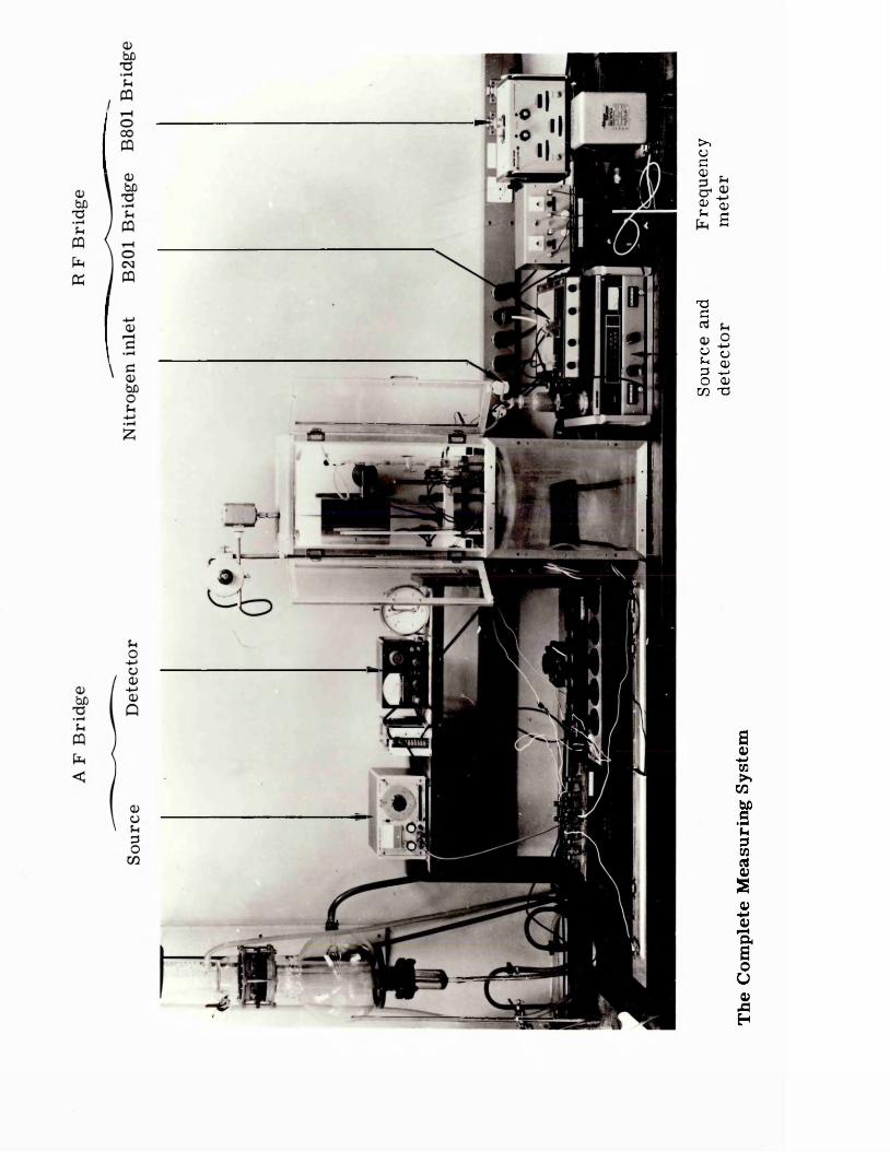
(iii) The Complete Measuring SystemA diagram of the complete measuring system is shown in

Figure 2.1. The Wheatstone bridge circuit was connected to the low-frequency electrodes of the conductance cell and the high-frequency electrodes were connected to the circuit for I’adio-frequency measurements, incorporating either the B201 or B801 bridge and a source and detector,

The bridge source and detector used in the radio­frequency circuit were combined in the Wayne-Kerr SR268 unit. v/hich is especially suitable for use in conjunction with the B801 and B201 bridges. The SR268 unit is a general purpose bridge source and null detector covering the frequency range

- 1*8 -

FIGURE 2.1

BLOCK DIAGRAM OF

MEASURING CIRCUIT

& :X Y

WAYNE- SOURCE

KERR AND

B R 1DGE DETECTOR

- 49 ~

100 KHz to 100 MHz* This frequency range is covered in nine hands, and the source and detector tuned circuits incorporate push-button attenuators* These are provided to control the source output level and the detector input sensitivity and a meter facilitates accurate visual detection of the null point.

The source output was tuned to the desired frequency with a crystal-controlled frequency meter, type CKB-74028, with an accurancy of about 0.02>o. Over a period of hours, a slight drift in the frequency of the output was noted and for this reason, the oscillator was re-tuned for each set of measurements. All external leads in the radio frequency apparatus were coaxial cables joined to the screened coaxial connectors. The power supply to all instruments was taken from a 50 Hz stabilised power suvjply (Advance Voltstat type C W 250A), giving 240 volts r.m.s. at 50 Hz.

The general layout of the instruments and apparatus described in these sections is illustrated in the Plate on the next page.

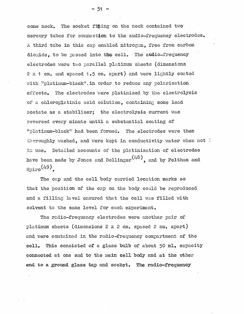
(IV) The Conductance CellThe conductance cell used in this work v/as designed

to enable conductance measurements to be made at both audio- and radio-frequencies. The cell is illustrated in Figure 2,2; the compartments were connected by thick-walled Pyrex glass tubing.

The audio-frequency compartment consisted of a cylindrical cell bodjr, of about 250 ml. capacity, with a ground glass

>> o c 0> .

0> CDu s

T3G

2 « « 0 3 -2 O 0) CO T3

The

Com

plet

e M

easu

ring

Sy

stem

- 51 -

cone neck. The socket filing on the neck contained two mercury tubes for connection to the audio-frequency electrodes. A third tube in this cap enabled nitrogen, free from carbon dioxide, to be passed into the cell. The audio-frequency electrodes were two parallel platinum sheets (dimensions 2 x 1 cm. and spaced 1.5 cm. apart) and were lightly coated with "platinum-black5', in order to reduce any polarisation effects* The electrodes were platinised by the electrolysis of a chloroplatinic acid solution, containing some lead acetate as a stabiliser; the electrolysis current was reversed every minute until a substantial coating of "platinum-black” had been formed. The electrodes were then thoroughly washed, and were kept in conductivity water when not in use. Detailed accounts of the platinisation of electrodes have been made by Jones and Bollinger and by Deltham andSpiro^^*

The cap and the cell body carried location marks so that the position of the cap on the body could be reproduced and a filling level ensured that the cell was filled with solvent to the same level for each experiment.

The radio-frequency electrodes were another pair of platinum sheets (dimensions 2 x 2 cm. spaced 2 cm. apart) and were contained in the radio-frequency compartment of the cell* This consisted of a glass bulb of about 50 ml. capacity connected at one end to the main cell body and at the other end to a ground glass tap and socket. The radio-frequency

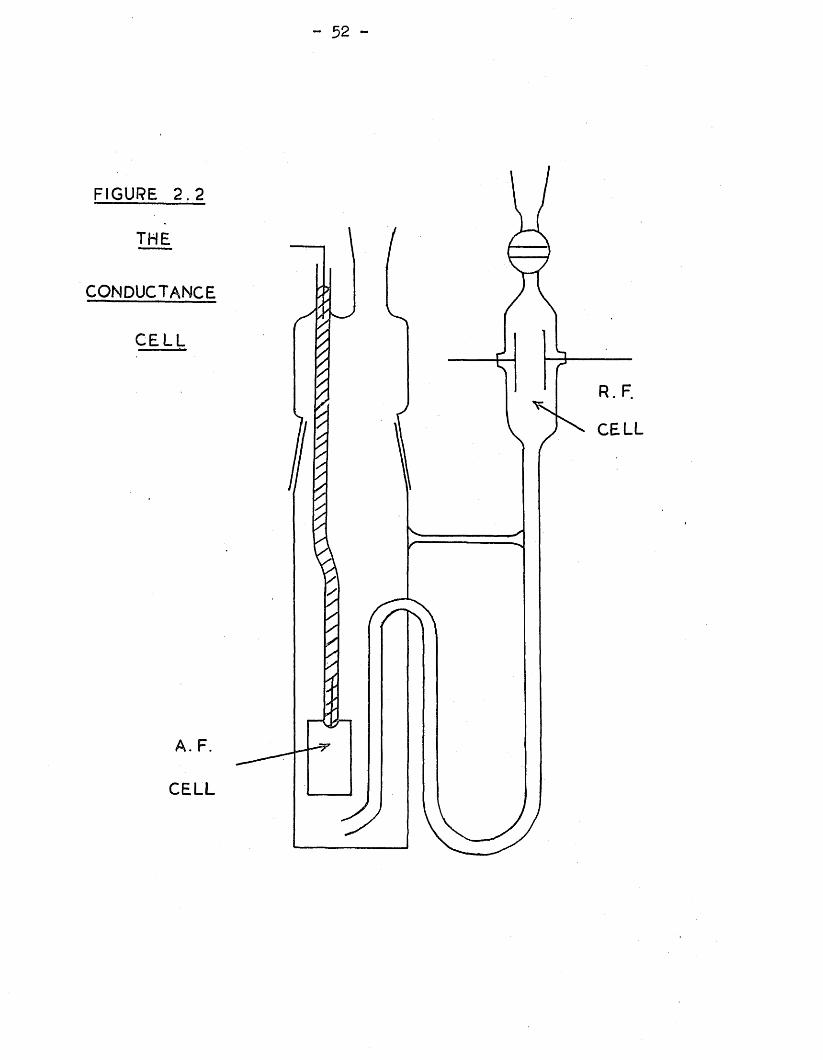
- 52 -

FIGURE 2 .2

THE

CONDUCTANCE

CELL

CELL

CELL

~ 53 -

electrodes were not platinised since polarisation effects were unlikely to occur at the high frequencies used,.

The conductance cell was used in the following way:Prior to the measurement of audio-frequency conductances, nitrogen was passed into the audio-frequency cell through the inlet above the glass tap* An opening positioned just below the audio-frequency electrodes enabled nitrogen saturated with water vapour to pass between them while measurements were not being made. The nitrogen flow mixed the solution thoroughly during thermal equilibration' of - the cell and contents. When the radio -frequency measurements were made, the solution was forced up to the radio frequency compartment by passing nitrogen into the main body of the cell* This compartment was allowed to fill completely and the glass tap above it was closed when the solution had reached the required level, leaving the electrodes in the solution.

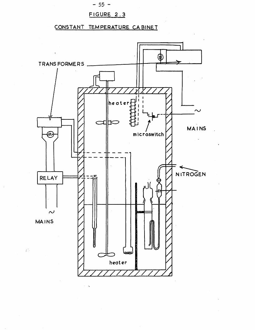
(V) Temperature Control,The conductance cell and its contents were maintained at

25*00 + 0.01°G by means of a constant temperature cabinet specially designed and constructed for this work. The cabinet was made from aluminium and efficient insulation was obtained from one inch thick polystyrene sheet lagging,'

The lower half of the cabinet contained a glass tank of about 30 litres capacity which was filled with light transformer oil, Jones and J o s e p h s h a d found water to be

- 5L ~

unsuitable for this purpose since the resistance of the cell varied with the frequency of the signal in the bridge. The oil bath was heated using a 200 watt heating coil, and temperature control was maintained using a contact thermometer regulator connected to a Sunvic Relay. The oil was stirred efficiently by means of a paddle stirrer driven by a Baird and Tatlock electric motor. A cooling coil was immersed in the bath for use during very hot weather. The bath was set to 25.00°C with a standard calibrated thermometer graduated in 0.01°C divisions, No temperature difference between the various parts of the bath could be detected with this thermometer. With the above arrangement the temperature of the thermostat could be maintained at 25.00 + 0.01°C.

The temperature of the air above the oil bath maintained at 25.0 + 0.1°C by means of a 50 watt heater connected to an air" bellows microswitch (obtained from Burgess Microswitch Ltd.). The air was circulated using a fan powered by the oil stirrer motor. Indicator bulbs were incorporated in the circuits to show when the air and oil heater circuits were switched on.

The conductance cell was placed in the oil bath through two d.ouble thickness perspex doors in the upper half of the cabinet. The cell was clamped in the bath close to one side of the cabinet so that the length of the leads from the radio- frequency electrodes could be kept to a minimum. It had been found that the use of leads more than one inch long resulted

- 55 - FIGURE 2.3

CONSTANT TEMPERATURE CABINET

TRANS FORMERS

h e a t e r

MA1NSmicroswitch

NITROGENRELAY

MAINS

heater

- 56 -

in a sharp decrease in the sensitivity of the bridge when used at frequencies above 10 MHz, although the resultant conductance reading was not affected. The measuring leads from the audio-frequency Wheatstone bridge Here dipped into two small tubes of mercury’in the oil bath. Two further leads from these tubes were dipped in the mercury in the audio-frequency electrode tubes. With this arrangement, heat losses from the audio frequency cell to the bridge via

/ i j - \the leads Y/ere kept to a minimum

PART II SECTION 2 MATERIALS

- 58 -

(i) Conductivity WaterThe conductivity water used throughout this work was

prepared as follows. Freshly prepared distilled water was passed through an Elgastat ion exchange column and the water collected was then passed through a column of i?Bio-deminrolit“ ion exchange resin. This consisted of a mixture of strong-acid and strong-base resins and was supplied ready mixed by the Permutit Company, Ltd. The water prepared ty this methodgenerally had a specific conductance in the range (0.4-0,&)

•*•(5 —1 —1 ox 10 ohm cm. at 25 C. The conductivity water wasfreshly prepared each day and was kept under nitrogen in 21. stoppered flasks. When filling the conductance cell, the water was first warmed to 25°C since it was found that this greatly decreased the time required for thermal equilibration of the cell and contents, and the thermostat.(ii) Solutes

Potassium choride. ”AnalaRw grade potassium chloride was recrystallised three times from conductivity water, dried at 110°C and then heated to dull red heat in a platinum crucible. The purified salt was allowed to cool in a desiccator, where it was finally stored in a stoppered bottle.

Magnesium Sulphate. **AnalaR-! grade magnesium sulphate heptahydrate was recrystallised three times from conductivity water and dried at 140°C. After grinding, the purified salt was dried to constant weight as the.anhydrous form at

^ 5 9 "

o (51 )320 C w . The salt was analysed for magnesium hy titrationwith the disodium salt of ethylene diamine tetracetic acid, « (62)(h.D.T.A.) using Brichrome Black T indicatorw .

Found: 20.23% MgTheory, for MgSO^ : 20.20%MgManganese '(II)-.Sulphate. wAnalaR” grade manganese

sulphate tetrahydrate was-recrystallised three times fromconductivity water and dried to constant weight at 103°Cas the monohydrate,a definite weighing form that is not

( 66)particularly h y g r o s c o p i c T h e composition of the salt was determined, hy analysis for manganese hy titration with E.D.T.A, and hy thermogravimetric analysis (T.G-.A.) for hydration using a Stanton Thermohalance (lOmg. full scale).

Found hy E.D.T.A. titration: 3 2.23% MnThe or y. f or MnSO^. Ii20: 32.51 % MnRecorded weight loss hy T.G-.A.: 10.36%Theoretical weight loss for MnSO^. K^O: 10.63% H^OMagnesium m- henzeaedisulphonate (MgBDS). This salt was

prepared, firstly hy purifying m~ henzenedisulphonic acid (Kodak Reagent, technical grade) hy hoiling an aqueous solution of the acid with decolourising carbon. Barium carbonate was then added to the filtered solution. The harium m- henzenedisulphonate (BaBDS) which formed remained in solution and some harium sulphate was precipitated due to the presence of sulphuric acid impurity. The harium sulphate was filtered off and the BaBDS precipitated hy the

- 60 -

addition of acetone. The BaBDS was dried, weighed and dissolved in conductivity water and a stoichiometric weight of magnesium sulphate (purified as ahove) was added* The harium sulphate formed was filtered off and the MgBDS so obtained was recrj stallised three times from conductivity water* An aqueous solution of the purified salt-was tested for the presence of harium and sulphate ions* The purified salt was dried to constant weight at 90°C* Analysis for magnesium content hy E.D.T.A* titration and for water content hy T.G.A* showed that the MgBDS was in the form of a definite 3i hydrate*

Found hy E.D.T.A* titration: 7*^8^ MgTheory for MgBDS* 3*5 HgO: 7*52/b MgRecorded weight loss hy T.G.A*: 19*10ysTheoretical weight loss for MgBDS* 3*5 H20 = 19»-47/& H20Duplicate analyses hy E.T.A* titration agreed towithin 0.02% of the mean*Manganese m- henzenedisulphonate (MnBDS). The preparation

of this salt was similar to that of MgBDS. In this case,BaBDS was prepared from the crude m- henzenedisulphonic acid and the stoichiometric weight of purified manganese ( IX )

sulphate was added. The MnBDS prepared in this way was recrystallised three times from conductivity water and an aqueous solution of the purified salt was tested for the presence of harium and sulphate ions. The purified salt was dried to constant weight at 90°C and analysed for

- 61. -

manganese content "by n,D.T,A, titration and for hydration by T. G-,A, The MnBDS was found to he in the form MnBDS, £jHqO

Found hy 33.D.T.A. titration: 15*11/o MnTheory for MnBDS, 15*12>o MnRecorded weight loss hy T,G-.A,: 19.60$Theoretical y/eight loss for MnBDS, IgL O = 19*75$ H^O Repeat analyses hy titi*ation differed hy no more than 0,02$ from the mean,

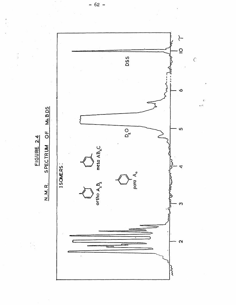
Characterisation o^ tj.ie_ _m~ henzenedisulnhonatesThe manganese and magnesium salts of m- henzenedisulphonic

acid were further examined in order to eliminate the possibility of any substantial quantities of the ortho- and para- isomers being present. The nuclear magnetic resonance spectra of MnBDS and MgBDS dissolved in deuterium oxide were recorded on a Perkin 33liner RlO 60 MHz nuclear magnetic resonsmce spectrometer using sodium 2,2- dimethyl -2-silapentane. sulphonate (DSS) as a reference. The sx ectra of the two corny)ounds were very similar and in both cases they exhibited an asymmetric series of ]?eaks in the 2^ region for aromatic protons as shown in Figure 2 If we use the convention for the labelling of aromatic nucleii^” , the three i30ssihle isomers correspond to the following systems: A^B^ (ortho),ABgC (meta), and A^ (para). In the case of the A£Bg and A^ systems, a high degree of symmetry is to he exiDected in the splitting xoatterns. HoY/ever, in both the si>ectra recorded, the pattern is decidedly asymmetric, and in this case could

- 62 -

04

llJOZ3oLL

<0aCOX

Li.o

23cch-oLlJaco

cc2z

cn

CO

a .

CO

04

~ 63 ~

only correspond to the A C case# This observation does not eliminate the possibility of the existence of the other isomers in the prepared salts but the indication is that the meta­isomer is in excess*

Additional evidence for the excess of the meta- isomer was provided by an examination of the infra-red spectra of MnBDS and MgBDS. The infra-red spectra were recorded using nujfcl mulls of the salts in the wavelength range 2-1,5 microns.In general, the 5-6 micron region of the spectra of benzenoid compounds contains weak overtone or combination absorption, bands of low intensity. These bands are characteristic of the type of substitution on the aromatic ring, and provided no interfering bands are present, they provide a reliable indication of the substitution pattern. Three weak bands were observed in this region at 5.56, 5*25 and 5.06 microns,

(93 )corresponding to a meta - disubstituted benzenoid compound'The remainder of each spectrum was generally characteristic

(55)of benzene sulphonates' .Thus the meta isomers -were not shown to be exclusively

present in the BDS salts but it was concluded that these isomers were, at least, present in large excess over the ortho- and para- forms.Preparation of stock solutions

The stock solutions were prepared by weighing the required amount of the salt under examination in a small glass tube.This was then introduced into a flask containing a known

— 6l(- —

weight of conductivity water, weighings were made to + 0.0001 g. and buoyancy corrections were applied throughout. A fresh stock solution Y/as made up for each experimental run.

PART II SECTION 3

EXPERIMENTAL TECHNIQUES

- 66 -

(i) Measurement of Audio-Frequency ConductanceThe audio-frequency conductances of the electrolyte

solutions under consideration were determined hy measurements of the resistances of the solutions. Before starting an experimental run the conductance cell was first cleaned, by passing steam through the cell for half an hour. The cell was then dried and weighed. Nitrogen was passed into the cell-, which was then filled with conductivity water (prepared at 25°C) up to the location mark. The cell and contents were re-weighed; a buoyancy correction was applied to the weight of solvent.

The cell was then firmly clamped in the thermostat and left to reach thermal equilibrium whilst a slow stream of nitrogen> saturated with water vapour, was passed through the cell. The purpose of the nitrogen stream was threefold: toprevent contamination of the solvent and solutions by carbon dioxide from the atmosphere, to facilitate mixing of the solutions and to inhibit electrolyte adsorption on the electrodes. The passage of nitrogen appeared to be successful in all these respects, but it was noted that resistances of the solutions appeared to decrease markedly after the nitrogen stream had stopped. On passing nitrogen again the resistances increased. This inconsistency in resistance readings was only observed for the most dilute solutions used. In general, the phenomenon of resistance change of an aqueous solution after the solution has ceased to be agitated has been noted by a

(56 57)number of workers' it has a.lso "been observed in(58) (59)solutions in methanol' , formamide , and dimethyl-

formamide^^. This effect was termed the "shaking effect*5by P r u e ^ \ who concluded that the phenomenon was probablycaused by concentration of electrolyte at the polar walls ofthe cell due to glass surface ion-exchange, /mother possible

/ - V

explanation is carbon dioxide contamination of solutions , but it is probable that this effect is not specifically due to carbon dioxide absorption. Prue recommended that the ^shaking effect” could be minimised either by waxing the interior of the cell or by making the diameter of the electrode chamber considerably larger than, the diameter of the electrodes In this work it was found that both these safeguards had disadvantages in cell constant measurement and cell design* Consistent resistance readings were obtained by balancing the bridge imme^ately after the nitrogen flow had been shut off. '..hen no readings were being taken, the solution was always agitated by a slow stream of nitrogen.

The conductivity water usually attained thermal equilibrium after one hour in the thermostat. After this period, resistance readings were constant for up to eight hours and so it was assumed that the resistance of the solvent would remain constant for the duration of a run. The resistance of the solvent was measured using the 55 shorted55 Y/heatstone Bridge circuit. Solutions of the electrolytes being studied were made up in the cell by the addition of small quantities of

- 68 -

stock solution from a syringe which was weighed before and after the addition. Nitrogen'was passed while the addition was "being made, and the solution was then mixed until the resistance of the solution was constant (about half an hour).

The following procedure was adopted for the measurement of the resistance of a solution. The resistance of the cell was first determined approximately by adjusting the resistance and capacitance boxes. The gain of the detector was then increased and two null positions on the slide wire were found corresponding respectively to the usual circuit of the bridge, and that with the leads to the Ratio arm reversed. These balance points were then redetermined, the solution being mixed by nitrogen between each reading. The arithmetic mean of the resistances measured was then taken to be the resistance of the solution.

The frequency of the current used was 11lls accurately sinusoidal. Possible errors due to polarisation were checked by taking series of readings at 1KHz and 3hHz. The differences between readings made at these frequencies were never more than 0mQ2% and so it was assumed that for the electrolytes and concentrations studied, polarisation effects could be neglected. The concentration of the solution used was calculated from the known weights of stock solution and solvent used.The concentration was converted to volume concentration using the density of water as 25°C as 0.99707^“ * The effect of the very small amount of the solute on the density of the

- 69 -

solution was neglected since it contributed an error much lessthan the error associated with making up the solutions hyweight. The molar conductance of the electrolyte was thendetermined hy the equation:

A = (/ R - fes) x cell constant x 10^ .......... (2.1 )concentration (m )

where R is the resistance of the solutionRs is the resistance of the solvent.

The cell constant was determined as described below, hohydrolysis corrections were applied to the electrolytes inthis investigation since no pH variation was found whensolutions were made up as in a normal conductance run, i.e.starting with solvent and adding portions of the stocksolution.

(ii) The Cell ConstantThe cell constant of the audio-frequency cell was found

hy measurement of the conductances of a series of potassiumchloride solutions of known concentration whose resistancesfell in the required range (800 - 6000 ohms). The equivalentconductances were calculated from the semi-empirical equationof Lind, Zwolerifc and Fuoss^^:

A = 1^9*93 - 94.65 c2 + 58.74 c log c + 198.4c .....(2.2)This equation represents the equivalent conductances of

potassium chloride solutions in water, at 25°C and at any-1concentration up to about 0.012 mole 1. , with an accura&cy

of about 0.013 o. The coefficients of the c2 and c log c terms

70

xiere calculated from tlie Fuoss-Onsager (1935) equation using a dielectric constant of water of 78.54 and viscosity of water of 0*008929. The limiting conductance and coefficient of the c term were 'weighted averages of nine sets of data for the conductances of dilute potassium chloride solutions, hy various

/ r p- \workers, hased on the Jones and Bradshaw standards' .

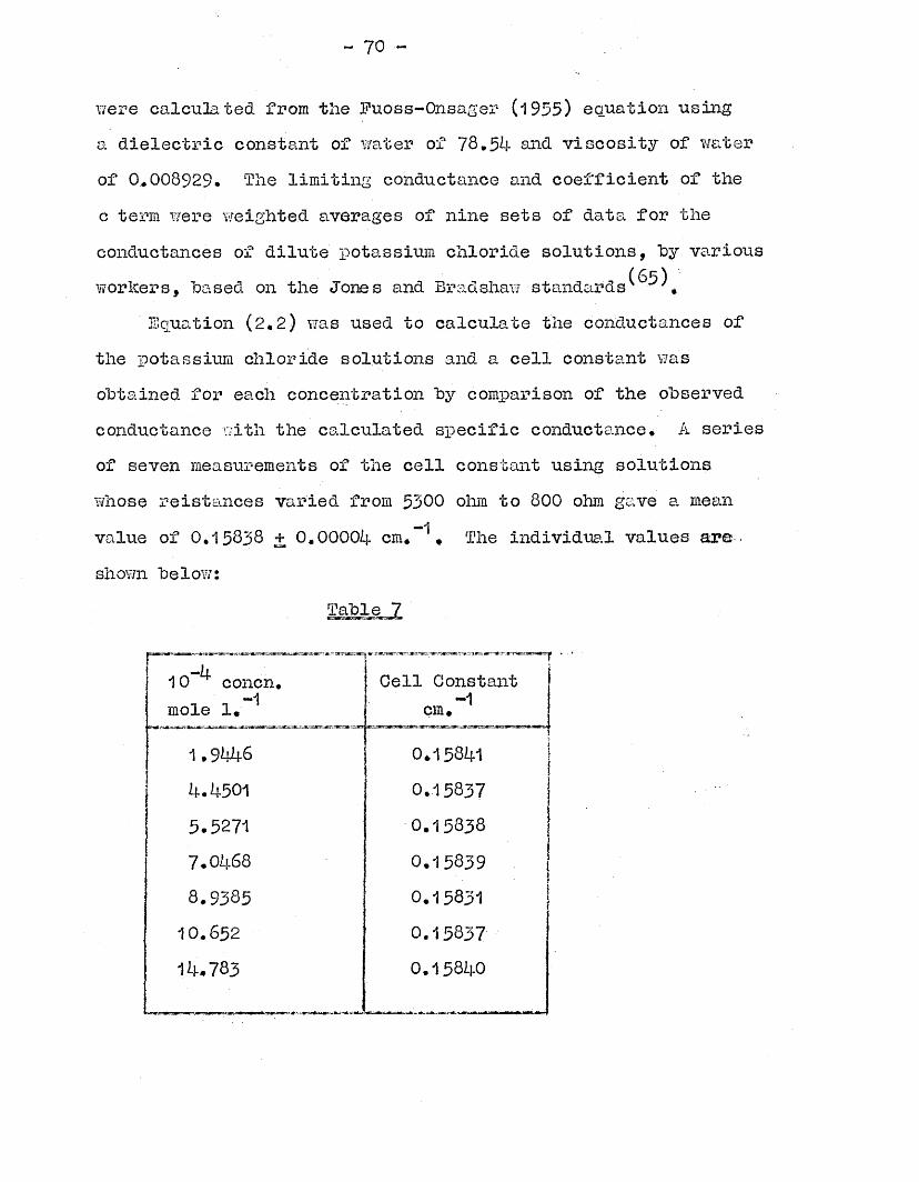
Equation (2.2) was used to calculate the conductances of the potassium chloride solutions and a cell constant was obtained for each concentration hy comparison of the observed conductance with the calculated specific conductance* A series of seven measurements of the cell constant using solutions whose reistances varied from 3300 ohm to 800 ohm gave a mean value of 0.15838 + 0.00001}. cm. * The individual values are ■ shown below:

Table 7

conczimole 1

1 .9446 0.15841

5.52717*04688.938510.65214.783

0.158390.158310.158370.15840

~ 71 -

(iii) Measurement, of Radio-Frequency ConductanceThe measurement of conductance at radio-frequencies

involved the use of a reference electrolyte* The radio- frequency compartment of the conductance cell was used for hoth reference and test electrolytes and this obviated the need for knowledge of a cell constant., which may well he expected to vary with frequency. The reference electrolyte used was potassium chloride. This was assumed to he completely dissociated in the solutions used and its variation of conductance with frequency was computed using the Falkenhagen- Le i s t—Ke Ihg e qua t ion .

The experimental technique was as follov/s: The cleaned,dried and weighed conductance cell was filled to the appropriate level with conductivity water. The cell and contents were then weighed and the cell was clamped in the thermostat. After thermal equilibration the resistance of the water was measured at 1 KHz. A weighed amount of stoch solution of the electrolyte was then added and the audio­frequency resistance of the resulting solution was measured after mixing and equilibration. The SR268 oscillator-detector, connected to the appropriate Wayne-Kerr bridge, was. tuned to the desired frequency of measurement using the heterodyne frequency meter.

Nitrogen was passed into the main cell compartment until the solution rose to the required level in the radio-frequency cell, with the radio-frequency electrodes completely immersed.

- 72 -

The W'ayne-Kerr bridge was then balanced, the sensitivity of the gain control being increased as the balance point was approached. The solution was then pumped down to the main cell body, mixed with a nitrogen stream and allowed to attain thermal equilibrium. The procedure was repeated several times to give a series of audio-frequency resistances and corresponding radio-frequency bridge readings. The arithmetic mean of each set of values was then taken. The solution was removed by blowing it to waste with nitrogen the cell was washed thoroughly with conductivity water until the conductance fell to that of fresh conductivity water. The cell was then filled with conductivity water and left to reach thermal equilibrium.

The solvent conductance was measured and potas&um ch/oride stock solution was added until the audio-frequency resistance of the solution fell to approximately that of the earlier electrolyte solution. The audio-frequency resistance and radio-frequency bridge reading were measured as before.By the addition of drops of potassium chloride stock solution or conductivity water, the conductance of the solution could be altered very slightly and values of the radio-frequency bridge reading (and the corresponding 1 KHz resiw tanCes) were obtained, which bracketed the radio-frequency bridge reading of the electrolyte solution. In this way, a calibration graph could be constructed of resistances at potassium chloride solutions at 1 KHz to the corresponding radio-frequency: bridge

- 73 ~

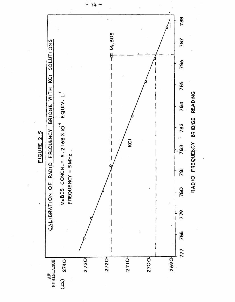
reading. A linear plot was usually obtained, and a typical

solution of MnBDS at 5 MHz* The radio-frequency readings were made using the B201 Bridge# From this graph it can he seen that the point for the MnBDS solution lies ahove the potassium chloride graph# Thus for any pair of potassium chloride and MnBDS solutions with the same audio-frequency resistance, the MnBDS has a greater radio-frequency conductance reading than the potassium chloride#

The information provided hy these measurements and the calibration graph was used to calculate the percentage dispersion and hence the radio-frequency conductance. As an example, the calculation for the MnBDS solution at 3 MHz will he given:

The MnBDS solution had an audio-frequency resistance of 2717*1 ohms with a corresponding radio-frequency dial reading of 786.4 on the B201 bridge. The potassium chloride solution having the same radio-frequency dial reading had a 1,KKz resistance of 2696*4 ohms, from the calibration graph. The dispersion of the MnBDS solution was then calculated from the

where X was the resistance equivalent to the B201 bridge reading (i.e. the radio-frequency resistance). In order to calculate X it is necessary to know the percentage conductance dispersion of the potassium chloride solution at 5 MHz. This was found by first determining the concentration of the potassium chloride solution with an audio-frequency resistance

graph is shown in Figure 2.3 for a 3*2168 x 10 equiv. 1

relation: (2.3)

- Ik

co

inCM

CM

Li-

LL

Q O r

oCM CM

Pq CQ <ij Hi ?

RADI

O FR

EQUE

NCY

BRID

GE

REA

DIN

G

- 75 -

of 2696.4 ohms. The specific conductance of this solution was—R —1 —icalculated to he 5*617x10 ohm ‘ cm* > after correction for

the solvent conductance.Using the Onsager limiting law,, values of equivalent

conductance, !\ and hence specific conductance, c/1000were calculated for a series of concentrations, c; in the range10 ^ to 10~^ equiv. 1. and a graph was constructed of

jlagainst c2, The concentration of the potassium chloride~5 “1solution having a specific conductance.of 5*617x10 ohm

—■\ ~ —I_Lcm, Y/as interpolated from the J /c2 graph to he 3,81x101 - 1.equiv. 1*

writing the Onsager limiting law in the form:1000 K. = A0 " (A, A o + V c ........ iZ.k)c

and rearranging gives:o = -iooo K . .1 .............(2.5 )

Ao A1 A oFor aqueous potassium chloride solutions at 25°G,

A = 149*93* A. = 0,2292, and An = 60,32* Using the o 1approximate value of 3*61 x 10 ^ as a first approximation, toc, the c value Y/as recycled in (2.5) until constant. A constant

— 1j “ 1value of 3*793 x 10 ** equiv. 1. Y/as quickly obtained. Thisfinal value of c v/as then used in the Falkenhagen-Leist-Kelhg equation to calculate the percentage dispersion of the potassium chloride solution. In practice, the dispersion was interpolated from a series of graphs of dispersion (calculated hy FLK) against concentration for potassium chloride at various frequencies. An a value of 3*14 S. (the sum of the

- 76 -

+ — \ (90)crystallographic radii of K and Cl ions) v Y/as used inthe computation for these graphs which are illustrated inFigures 2*6 and 2*7. In this calculation the dispersion v/asfound to he 0.11$

Then the value of X will he given by:x - 2696.h x 100 = 2692.6 ohms.

(1 oo + 0.124.)

and so the percentage dispersion for MnBDS can he calculatedfrom (2.3) to he: V;;:

A (2717.1 - 2692*6) x 100^ = 0.90fo( 2717.1 )

The eq.uivo.lent conductance of MnBDS Y/as found to he 106*27at 13XHz, therefore the equivalent conductance at 3 MHz wascalculated to he:

A = 106.27 x = 107*23 ohm equiv.

The method of using a potassium chloride reference as described ahove does not require a radio-frequency cell constant to he measured. Moreover, any variations of cell constant with frequency or concentration^^ will he eliminated since hoth test and reference electrolytes are measured at the same frequency and at_approximately the same cell resistance. The disadvantage of the method is that the test electrolyte solution has to he replaced hy potassium chloride for each run; a simple and relatively quick dilution or concentration technique could not he used. However, the conductances of several concentrations of an electrolyte were determined at two or three frequencies for each run in order to obtain as

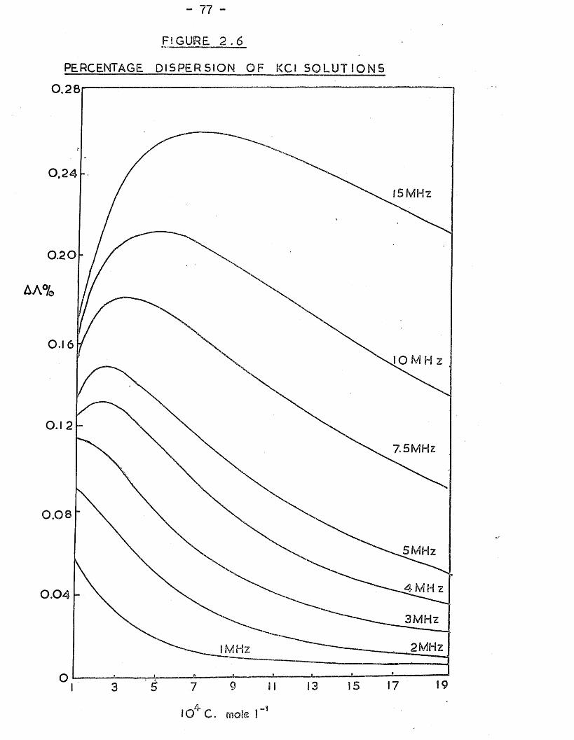
- 77 -

FIGURE 2.6

PERCENTAGE DISPERSION OF KC1 S O L U T I O N S0.28

0.2415MHz

0.20

0.16iOMH z

75MHz

0.08

5MHz

0.043MHz

2 MHzHz

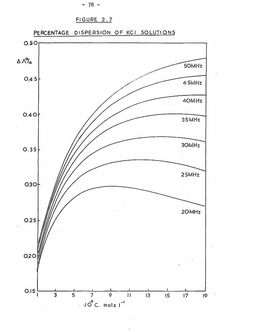
- 78 -

FIGURE 2.7

PERCENTAGE DISPERSION O F KCi SOLUTIONS0.50

A A °/(

0.4 5

0.4 0

0.35

0.30

20MHz0.25

0.20

0.154- »JO m

- 79 -

much data as possible from each experiment*Potassium chloride is particularly suitable as a reference

electrolyte. It is easily purified, completely dissociated in aqueous solution and the frequency dispersion of conductance of potassium chloride is always considerably less than the more highly charged salts investigated in this work^^#

PART III SECTION 1

TREATMENT OP RESUITS

- 81 -

The negative deviations of the phoreograms of bi-bi valent electrolytes from the limiting law may he attributed to ion association, described by the thermodynamic association constant, In the case of ion association, the conductanceequation chosen to represent the phoreogram of a given salt in a particular solvent is a function of the three parameters

A o anc a* ^ "this section to reviewthe various methods available for the computation of V A o and a from conductance data. It will be assumed that ion association consists of ion-pair formation only and so KA

je*j-

describes the equilibrium between free ions and non-conducting ion-pairs. This is a reasonable assumption for the concentr-, o'

ation range investigated in this work (0-0.0009 M) and for aqueous solutions. The methods of computation may be conveniently divided into two classes: extrapolation and minimisation. In the present work computer programs have been developed for extrapolation and minimisation techniques to analyse audio-frequency (iKHz) conductance data and conductances measured at radio-frequencies,

(i) Sxtrapolation Methods/ /* **7 \

The audio-frequency data of Dunsmore and James for magnesium sulphate will be used to illustrate the various methods of extrapolation used in this work. A A versus o'2 plot of this data is shown in Figure 3*1* The plot shows- systematic negative deviations from the Debye-Hilckel-

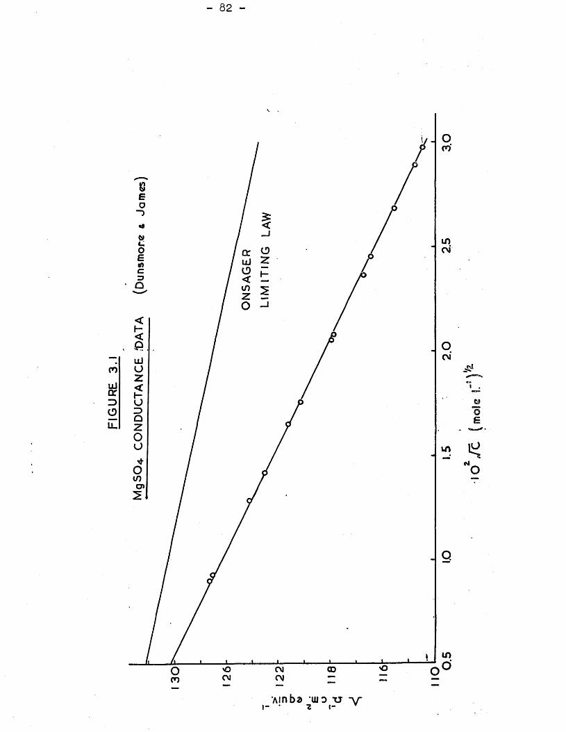
FIG

UR

E

- 82 -

co

in

CMCO

<slUo

- 83 -

Onsager limiting law, which is also illustrated in the graph, Davies attributed deviations of this kind to ion association effects and assumed that the free ions obeyed the limiting law with the introduction of the degree of dissociation, c*. :

A = «*( A o - (S1 A 0 + S2)(cxcf) (3 . 0

The degree of dissociation may be found by a series of successive approximations and so may be found from equation In the original calculations of Davies,the Debye-Huckel limiting la?/ (1 - i 5) was used for the mean ion activity coefficient of the free ions, but the calculation may be extended to include the ion size parameter, a, by use of the extended form of the limiting law (1 »1 6) or by the use of the Davies empirical equation:

“loS10f+ = Xs - 0 .3 1) .....(3.2)1 + 1 2 *31]

which corresponds to the choice of a = 4.3-S.The choice of a in these calculations will influence the

values obtained for K,• Prior knowledge of the value of /\A ois also required and this can bo conveniently set equal to the sum of the limiting ionic conductances, if known, For MgSO, , A Q = 133.07, from A 0(lig2+) = 53.05 ('69' and A o(S042_) = 80.02

The Davies method enables to be determined at eachconcentration, the final choice of K,, being made by

1*1.

- Qk -

extrapolation of a - c plot to c = Ot The method of successive approximations for K, forms the starting point forJr±alternative techniques that determine K^ and A from the slope and intercept respectively of a suitable extrapolation plot,

(71 )A method devised by Fuoss and Krausv / starts with the Debye-Hilckel-Onsager limiting law (3,1),.rearranged to give

ot = A ..(3.3)A„ - (s, A „ + s0 ) (o tc ) *

which is a cubic equation inoC . If, as a first approximation to cA , the Arrhenius value of cA = A / A 0 is substituted, this gives

ot ■= A (3.4)A o " ( s / A / ) ( c ^

Y/here S = (S A Q + iimiiin£ slope,A second approximation is then found by substitution of oi back into the denominator for -oC. in (3.3) :

c* = A ^ ....... .+-(3.5)2 A 0 - sCc^c)2

Iteration of this process causes a rapid convergence to a constant value of c£ , which can be witten as

©< = A / ( A 0P (y ) ) . . . . . v. . . . (3 -6)

85 -

where F(y) = k/3cos2(icos .y/2 )) ..••(3.7)and y = S.( A Q)~^2.(c A ) 2 ..............••.•(3.8)

(72 )F(y) values have "been tabulated by Fuossv ' for 0 ^ y 4 0-209y-2 -1corresponding to an upper limit of about 10 equiv.1,

Substitution of cX from (3.7) in the mass action equation (1.11+) and setting c' (mole 1. ) = c(equiv.l. )/z ;

p(y > = n + cAf± \ (3 .9 )A 0 z A 02F(y)

pThus a plot of F(y)/A against of\t, /F(y) will determine"TO “ .IC as the slope (K^/3 , ) an<3- A Q as 'the intercept (l/AQ).A preliminary value of A for this method can be obtainedby a freehand extrapolation of the conductance data. TheA Q from the extrapolation function (3*9) can then berecycled until a constant A Q value is obtained giving finalK. and A values,A o

The Fuoss-Kraus method depends on the limiting law.(7 ) . . .Shedlovsky J has proposed another extension of the limiting

law which was found to fit the data for 1 :1 salts in ?/ater-2 -1up to about 10 mole 1Q :

A = f \ - ( A / A 0)sc (3A0)If the observed conductance is set equal to the degree ofdissociation times the conductance given by (3.10), a

i_quadratic equation inc*,2 is obtained %

= 1 + S c ^ ^ (3.11)A A A 02

- 86 -

The solution of this quadratic may he written as :

c* = A S(y)/A0 .....

where S(y) = (y/2 + (1, + (y/2)2)2)2

(3.12)

(3.13)

with y defined hy (j>.8). Substitution of (3.12) into (1 ,14) gives :

+ c A S(y)f+'zK, A 2

Thus a plot of l/(AS(y)) against cAf, S(y) determinesand A 0 from the slope and intercept* The initial A Q

value can he determined from a freehand extrapolation of the conductance data, and can then he recycled. The S(y)

The Shedlovsky extrapolation was recommended for use in the

the effect of errors in 'concentration and specific conductance on K. and A for solutions of weak acids*A O

The Fuoss-Kraus and Shedlovsky techniques have their hasis in a limiting law conductance function! partial allowance can he made for ion size hy use of an activity coefficient equation such as the Davies or extended Debye- Hiickel law. However, a consistent extrapolation function needs to have a conductance equation incorporating a for

function has been tabulated hy Daggettof the Fuoss-Kraus and ShedlovskyA comparison

methods has shown that the two methods do not differAsignificantly for values of K, greater than 1000 l.molexA

pproximate range 1000^ K.yi . Kilpatrick

- 87 -

characterisation of the behaviour of the free ions. The extrapolation function most used in the present work utilises one of the extended conductance equations incorporating a, as described in Part I, The derivation of the function is as follows; The conductance equation is represented ass

A = f (c; A Q, a, z) ...... . (1 .21 )

and a degree of dissociation is introduced:

A = • <*f(<*c; A 0?a5 z) .....(1.22)

If this value of conductance is set equal to the experiment­ally measured value, A v * at concentration c, thenexp

= A 0X13 ....(3.15)A

At this point it is convenient to define a function where j6 - A / A > theno

** = A oz-p........ .................... .(3 .1 6)"fi A 0

substitution of (3*1$) into (1.1U) gives

P 1 + (0 A (iZPf±2) (Ka )A oxp Ao z0 ' ( AQb

..... (3.17)A plot of 00/A oxp) against (c Acxpf2/ W gives ICA/z Aq2 asslope and 1/a 0 as intercept, in applying this method, the activity coefficients were< calculated'usingvbhe extended

- 88 -

Debye-Hiickel equation with the same value of a as in the ...conductance equation. This extrapolation method wasprogrammed in Algol for an ICL 1905P computer. A basic flowdiagram of the program is shown overleaf and the various stepsmay be summarised as follows: The input data required is,a preliminary value of A 0? N pairs of conductances andconcentrations, c^A (i=l...N); M a-parametcr values,a .(;j=1 •».M); the valency of the electrolyte, z; the dielectric Dconstant of the solvent, D; its viscosity, • v ; the temperature,T, and, in the case of a frequency-dependent conductanceequation, the frequency at which measurements were made. Asa f irst approximation to the degree of dissociation, is setequal to 1 , and the concentration is modified fromstoichiometric to ionic. The theoretical conductance is thencalculated and cA is set equal to A. r / A * This value isexpthen compared with the earlier value of cA and the entirecalculation is repeated until successive values areconstant to within +0.0001. The quantities j6f )6/ A andexp2 are then calculated. This procedure is repeatedfor all N pairs of A and c and the values are treated byexpa standard least-squares procedure which yields an intercept,C and gradient, G. The A -value is recycled and the entire

r o

computation repeated until successive A 0“Valucs are constant to within +0,001 conductance units. The final values of K, ,A q and the standard deviation of the plot are then printed as output. These final values are independent of the initial

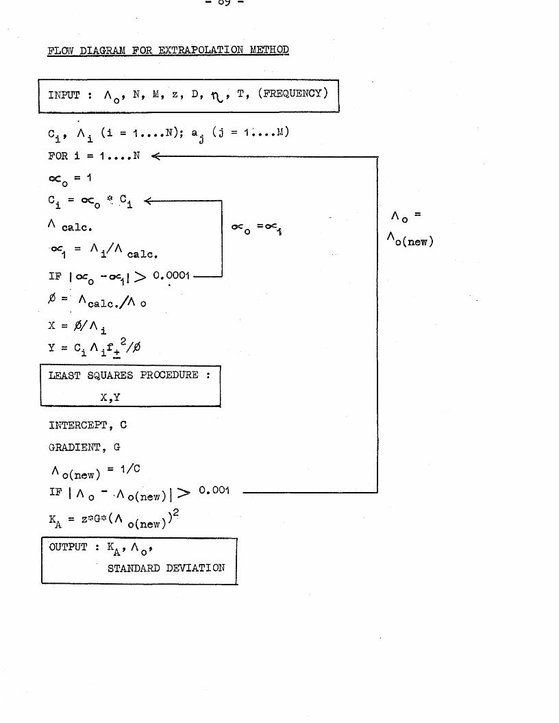
- oy -

FLOV? DIAGRAM FOR EXTRAPOLATION METHOD

INPUT : A 0, N> M, z, D, T> (FREQUENCY)

C. , A. (i = 1....N); a (j = 1....M)1 1 JFOR i = 1....N <------------------QC_ = 1C. = oc: # C.

A calc.- A^/A ca“LC>

IF | ocQ -o^j > 0.0001

^ ~ ^calc./A o X = fi/NA

=oC1

y = ci A ±f +d/j6

A o^o(new)

LEAST SQUARES PROCEDURE : X,Y

INTERCEPT, CGRADIENT, GA y = 1/C ''o(new;w U o A 0(neT/) | > °'00'1Ka = z*G*(A 0(new))2

OUTPUT : Ka> A q,STANDARD DEVIATION

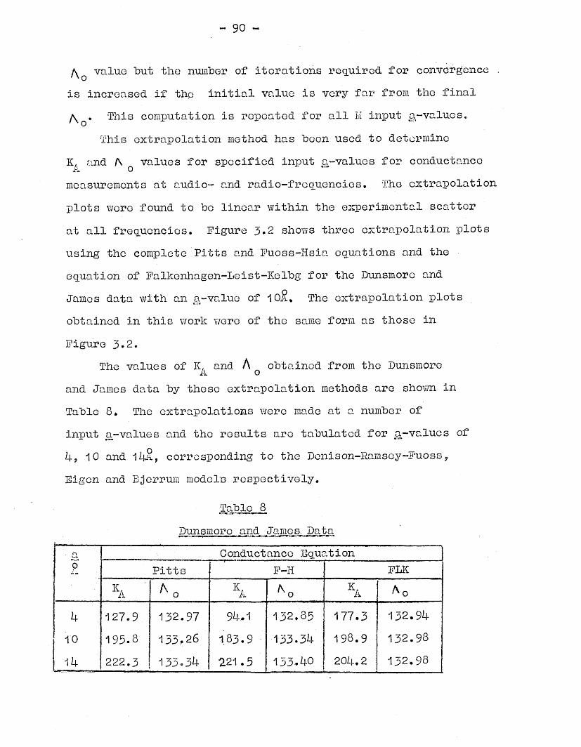
- 90 -

y\o value "but the number of iterations required for convergence is increased if the initial value is very far from the final

* 'This computation is repeated for all M input a-values*This extrapolation method has been used to determine

Ka and f\ values for specified input a-values for conductanceJri. Omeasurements at audio- and radio-frequencies, The extrapolation plots were found to he linear within the experimental scatter at all frequencies. Figure 3,2 shows three extrapolation plots using the complete Pitts and Fuoss-Hsia equations and the equation of Falkenhagen-Leist-Kelbg for the Dunsmore and James data with an a-value of 10.2, The extrapolation plots obtained in this work were of the same form as those in Figure 3.2.

The values of K, and A obtained from the Dunsmore A oand James data by these extrapolation methods are shown in Table 8* The extrapolations were made at a number of input a-values and the results arc tabulated for a-values of

10 and 14&> corresponding to the Denison-Ramsey-Puoss 9 Eigen and Bjerrum models respectively.

Table 8 Dunsmore and James. Data

■ a Conductance EquationP Pitts P-H ELK

ka ka A A o

k 127.9 132.97 94.1 132.85 177.3 132.9410 195-8 133,26 183.9 133.34 198.9 132.9814 222.3 133.34 221.5 133.40 204.2 132.98

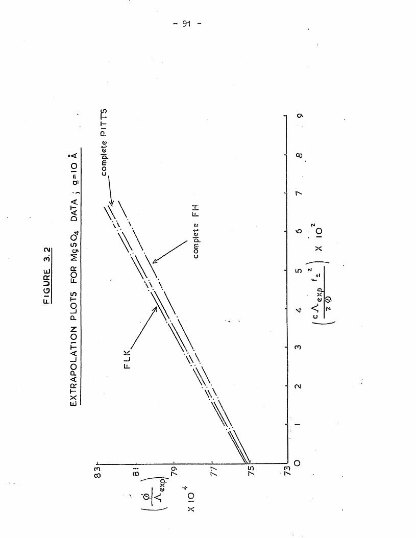
- 91 -

CMCOUJq:3OLL

o<O«Dt

<<Ca

dinC7>

q:Ollinh-Oazop<oa<orh-XLL)

CL

inma.

G O

dio • o

in *1v-Q-Xfc}U

CO

N

CM

O

"0.

x&<: o

X

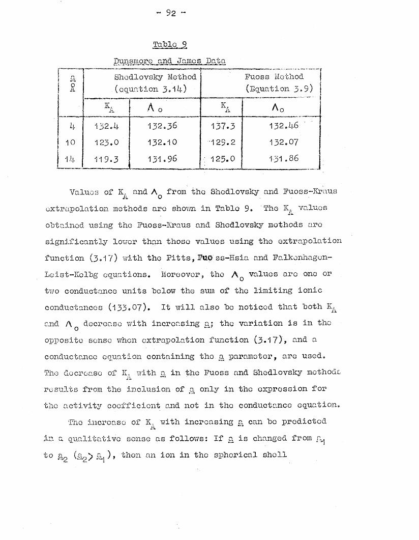
- 92 -

Dunsmore and James Data1 a

sShodlovsky Method . (equation 3*14)

Fuoss Method (Equation 3°9

JrL A 0 ka A q

L\. 132.14 1 3 2 .3 6 1 3 7 .3 132,^610 123.0 13 2 .1 0 1 2 9 .2 132,07

; 14 1 1 9 .3 1 3 1 .9 6 1 2 5 .0 131.36

Values of K, and A from the Shedlovsky and Fuoss-Kraus A oextrapolation methods are shown in Table 9* The values obtained using the Fuoss-Kraus and Shedlovsky methods are significantly lower than those values using the extrapolation function (3<w17) with the Pitts, Fup'ss-Hsia and Falkenhagon- Leist-Kelbg eq.uations. Moreover, the A Q values are one or two conductance units below the sum of the limiting ionic conductances (133.07). it will also be noticed that both K^ and A decrease with increasing a; the variation is in the opposite sense when extrapolation function (3.17), and a conductance equation containing the a parameter, are used*The decrease of K, with a in the Fuoss and Shedlovsky methods results from the inclusion of a only in the expression for the activity coefficient and not in the conductance equation.

The increase of K, with increasing a can be predicted in a qualitative sense as follows; If a is changed from a., to aQ then an ion in the spherical shell

- •9 3 -

b/3 7t( - a^), opposite in sign to a reference ion, wasformerly regarded as being free and will now be classed asassociated. Therefore the numerical value of shouldincrease, and this prediction is fulfilled according to thedata of Table 8. The dependence of upon a has beenpreviously treated in detail for a number of 2s2 salts byPrue, et al.^^ Values of from the Dunsmore and

oJames data, evaluated for a-values of 2 to 14 A have been plotted in Figure 3*3> which shows monotonic increases in K, for the three equations used. The first observation that can be made from Figure 3.3 concerns the very large variation of K^, according to the Pitts and Fuoss-Hsia equations, over the range of a-values studied. This observation adds weight to the argument of Prue, et al. that t!.«. an association constant cited without specifying also the other parameters involved and in particular d (i.e. a) is meaningless The indeterminacy of when a is not specified has also

(~7Q)been noted by Guggenheimv1'J mWhen the Falkenhagen-Leist-Kelbg equation is used in

the extrapolation method, the variation of K,, v/ith a is relatively small, and the values at 4.3» 10 and 14 2 are very close to the association constants evaluated for the Dunsmore and James data by Prue^^ using the equation of Leist^^. These two sets of results are shown in Table 10. Thus the variation of , and hence of A , with a must be very similar for both the FLK and Deist equations but significantly different from the values obtained by the

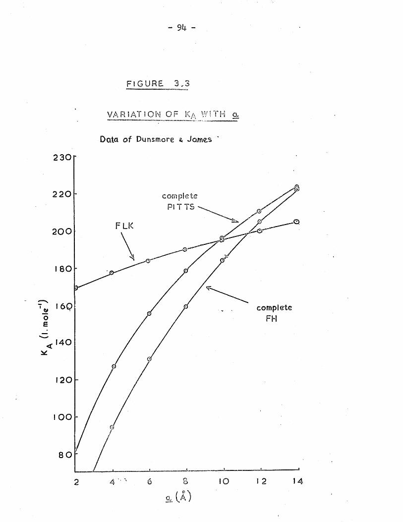
. mol

e

- 9k -

Data of Dunsmore 4 James

2 30r

220TS

200

I 80

I 60FH

140

120

IOO

8 0

SO I 2 1462 4

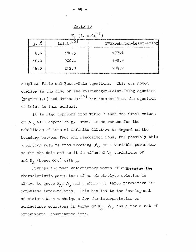
- 95 -

Table 10

IC (1. mole-1 )a, 2. F^lkenhagon- Leist-KgIbg

k.3 180.5 177.610.0 200. h 198.9Ako 0 212.0 20i|.»2

complete Pitts and Puoss-Hsia equations. This was notedearlier in the case of the Falkenhagen-Leist-Kelbg equation(Figure 1.2) and Matheson^^ has commented on the equationof Leist in this context.

It is also apparent from Table 7 that the final valuesof A will depend on a. There is no reason for the o “ —mobilities of ions at infinite dilution to depend on the boundary between free and associated ions, but possibly this variation results from treating A Q as n variable parameter to fit the data and so it is affected by variations of and (hence c* c) with a.

Perhaps the most satisfactory moans of expressing the characteristic parameters of an electrolyte solution is always to quote IC,, A and a since all three parameters arex A Odoubtless inter-related. This has led to the development of minimisation techniques for the interpretation of conductance equations in terms of K, , A and a for a set ofxx Oexperimental conductance data.

- 96 -

(ii) Minimisation MethodsIt has heen noted that hoth K, and A are sensitive toii o

the choice of the a - parameter. Extrapolation methodsprovide a useful means of evaluation of K, and A Q using apreselected range of a - values. However, in order to obtainan independent set of the three parameters K , A Q and a tocharacterise a particular electrolyte, it is necessary to usea minimisation method to treat the conductance data.

(13)Fuoss and Hsia analysed sets of data points c. ,A . (i = 1 ... N) in terms of , A and a as follows. An1 ' ii/ Oarbitrary value of K, was chosen of the correct order ofii.magnitude for the data under consideration. Then values ofA and a were found which would minimise the function:° p 2S ^ calc. ci* A o' ^ i (3.18)i=12Y/here S is the sum of the squared deviations between

(13)calculated^ ' and experimental conductances, and A calc, isthe theoretical conductance at concentration c^ using theparticular values K. , Ik*£\_7 o “

Then another value of the association constant Y/as tested 2and S was again computed. The process was repeated until the

minimising value of Kv Y/as bracketed. The minimising K, andi i.its associated A and a values were then taken to be the' o “minimising parameters between theory and experimental for theelectrolyte under consideration. In an alternative technique, 2S was computed for a number of a values and Y/as minimised

with respect to A and K,.* This was considered to produceo A

- 97 -

. . . (6 3,81*.)a sharper minimum * : i

These minimisation techniques were demonstrated hy Fuoss/gc gg 8"7 et al, * * ' to he useful evaluation techniques when

applied to some uni-univalent electrolytes. In theseinvestigations, the Debye-Hiickel limiting law (1.13) had heenused to calculate the activity coefficients of free ionsbecause ?}ions in contact are counted as pairs and long rangeinteractions between free ions cannot depend on the size of

(88 the ions hut only on their charges” . Thus a given value of the a. - parameter was used in A calc, hut a was set equal to zero in the expression for the activity coefficient. This not only introduces an inconsistency in the use of a hut isan unnecessary approximation. The use of the limiting law

(1 6) (89)has also heen criticised hy Prue et al.v'' } and hy Justice .A minimisation method has heen applied successfully to

conductance data of hi-hivalent salts hy Prue and co-workers^^and minimisation techniques were applied in the present workto evaluate 11 , a and A Q for each electrolyte and frequencystudied. The first program written for this method computedthe differences ( A calc. - A^) for incremental changes inK. , A an& a over suitable ranges. The values of the n o r'~parameters that minimised ✓ ( a , calc - A ) were ^ en

i=1 * 1found hy inspection. This program was used to analyse theaudio-frequency conductance data and an example of its structure is given in Appendix 1... The equations used in this type of program to obtain A calc, were the complete and

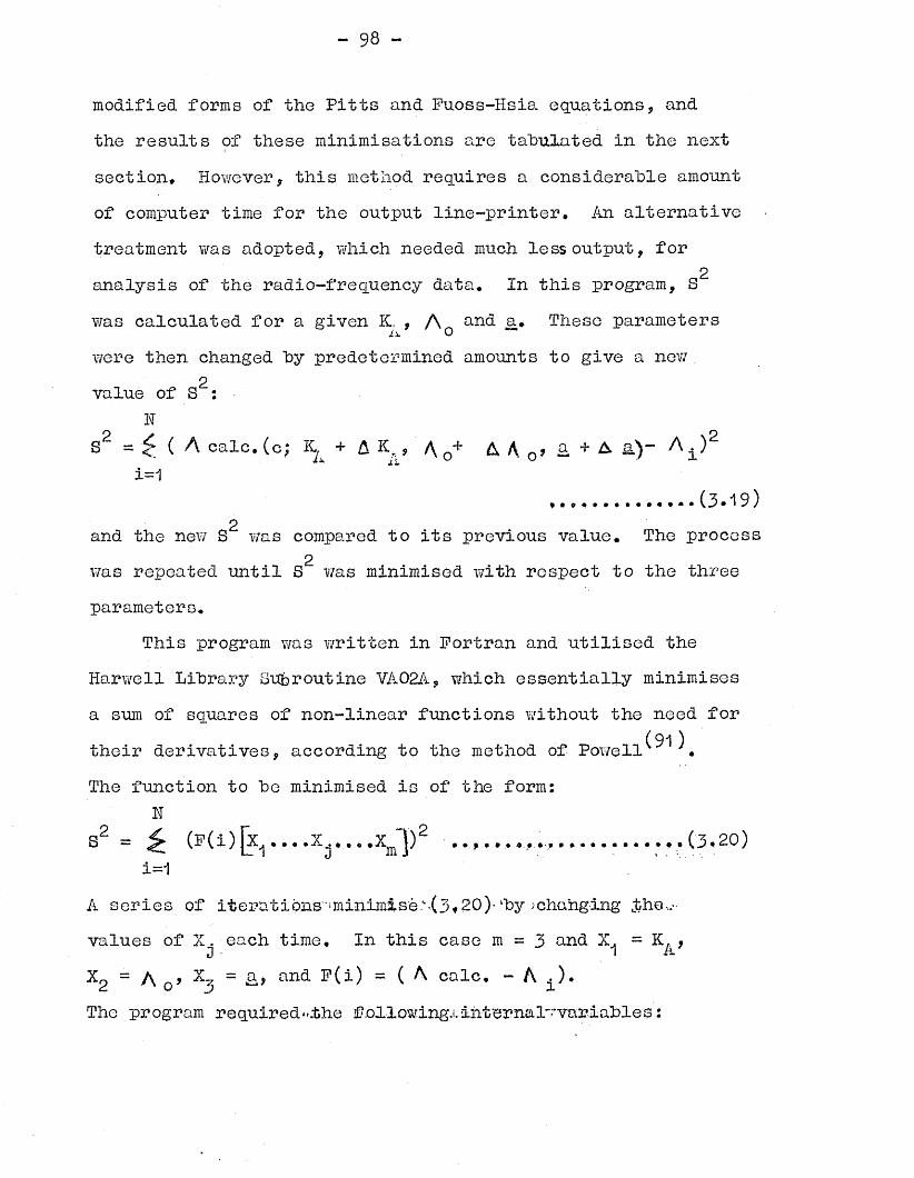
- 98 -

modified forms of the Pitts and Fuoss-Hsia equations, and the results of these minimisations are tabulated in the next section* However, this method requires a considerable amount of computer time for the output line-printer* An alternative treatment was adopted, which needed much less output, for

2analysis of the radio-frequency data, in this program, S was calculated for a given K, , an<3- a. These parametersii. o ""were then changed by predetermined amounts to give a new

2value of S :N

S2 = •<£ ( A calc* (c; K. + A , /\ A A , a + A &)- A ±)2ii.

1 = 1------------ (3.19)

2and the new S was compared to its previous value. The process2was repeated until S was minimised with respect to the three

parameters.This program was written in Fortran and utilised the

Harwell Library Subroutine VA02A, Y/hich essentially minimisesa sum of squares of non-linear functions without the need for

(91)their derivatives, according to the method of Powell •The function to be minimised is of the form:

3srs2 = ^ (E '( i ) {x i . . . . x j ------ X^)2 . (3 .20 )

i =1A series of it era t i bus • ■■ minimi s e" ■( 3 < 2 0) • lby > chang ing .the* • values of X . each time. In this case m = 3 and X. = K. ,0 1 ii.X2 = A 0> X3 = and F(i) = ^ calc, - A .).The program required-.the following.). internal~"var table s:

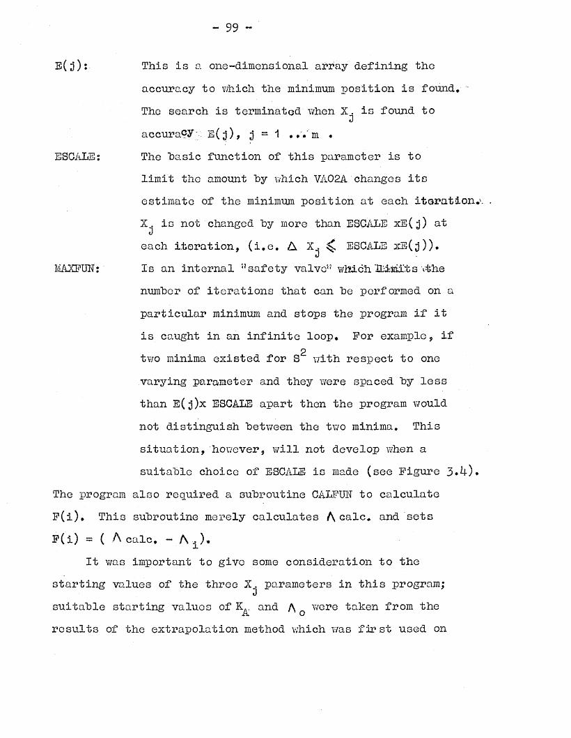
- 99 -

ESCALE;

MAXFUN:

E(3): This is a one-dimensional array defining theaccuracy to which the minimum position is found, -The search is terminated when X. is found to3accuracy;: E(j), 3 = 1 « ,. m «The "basic function of this parameter is tolimit the amount "by which VA02A.'changes itsestimate of the minimum position at each iterationsX. is not changed "by more than ESGALE xE(j) at 3each 'iteration, (i,e. A X . ^ ESCALE xE(j)).JIs an internal ”safety valve” which XDIiilis ithenumber of itei ations that can "be performed on aparticular minimum and stops the program if itis caught in an infinite loop. For example, if

2two minima existed for S with respect to onevarying parameter and they were spaced by lessthan E(3)x ESCALE apart then the program wouldnot distinguish between the two minima. Thissituation, 'however, will not develop when asuitable choice of ESCALE is made (see Figure 3»h)*

The program also required a subroutine CALFUE to calculateF(i), This subroutine merely calculates A calc, and setsF(i) = ( A calc, - A i)«

It was important to give some consideration to thestarting values of the three X. parameters in this program;3suitable starting values of KA. and A were taken from the

XT, Oresults of the extrapolation method which Y/as first used on

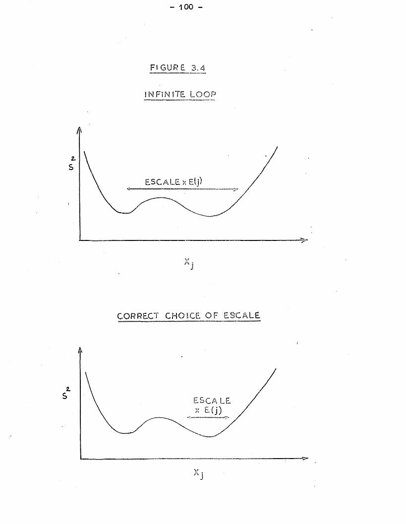
- 100 -

FIGURE 3.4

INFINITE LOOP

ESCALEx Elj)

CORRECT CHOICE OF ESC ALE

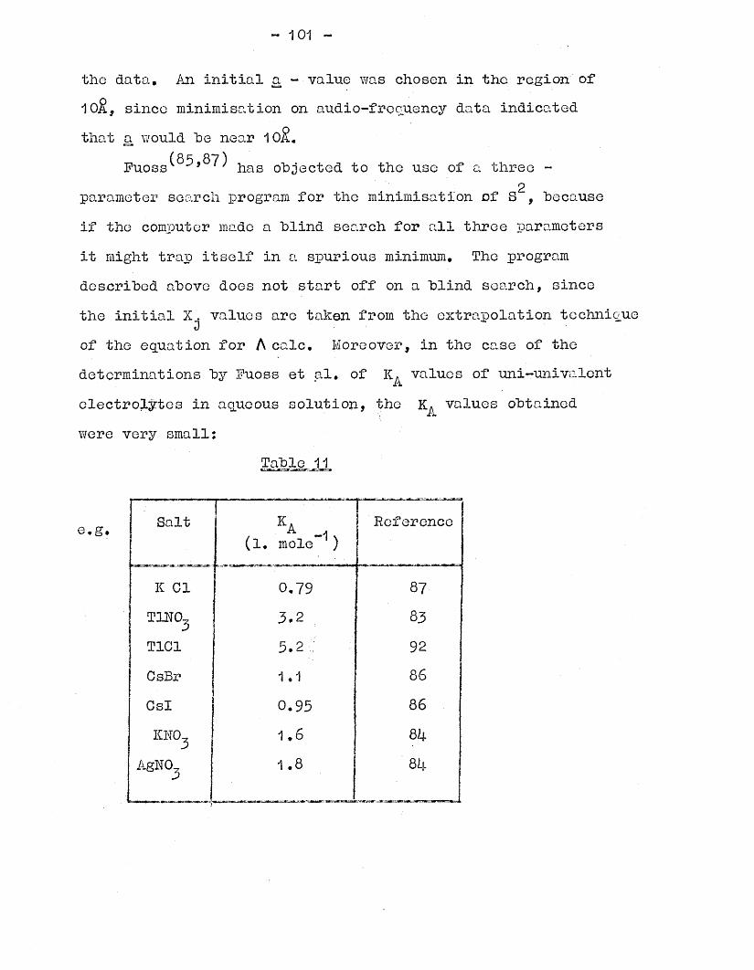
- 101 -

the data. An initial a - value was chosen in the region of10.&, since minimisation on audio-frcouency data indicatedthat a would he near 10$.

Ruoss^'^*^ has objected to the use of a three -2parameter search program for the minimisation of S , because

if the computer made a blind search for all three parameters it might trap itself in a spurious minimum. The program described above does not start off on a blind search, since the initial X. values are taken from the extrapolation technicjuet)of the equation for A calc. Moreover, in the case of the determinations by Ruoss et al. of values of uni-univalent electrolytes in aqueous solution, the E values obtained were very small:

Table 11

Salt-1(l. mole )

Reference

IC Cl 0.79 87T1RCL5 3.2 83T1C1 3.2 . 92CsBr 1.1 86Csl 0.95 86KNCa5 1.6 Qk

AgNO^ 1.8 Qk

- 1 02 -

The degrees of dissociation were very close to unity.In this case a three parameter program would produce thearithmetic minimising parameters hut the result would hewithout significance because of the lack of sensitivity of 2S to ^ as The shape of the minimum curve would also

be very dependent on the concentration range. In the caseof bi-bivalent salts, is not vanishing^ small and theS / relationship is still sensitive to variations in KThe ¥/ell-defined minima in Figure 3*5 were obtained for theconductance data of manganese sulphate measured in this work.Infinite loops were rarely encountered and sensible valuesof K , A and a were obtained for the 2:2 salts examined,A 9 o “ 9so long as attention was paid to the initial values of the X.. parameters and the choice of E SCALE. When the throa.-parameters- .were varied it was noted that A had the greatest effect ono2the value of S . This is to be expected since A q is theleading term in all the conductance equations. However, the

2^ corresponding to a minimum S was relatively insensitive to the values of the other two parameters; changes in /\Q of 0.02 conductance units were often obtained over the entire

& ji ranges studied.The VA02A minimisation program was used in this work

for the analysis of the conductancedata measured at radio­frequencies. It was found that the equation of Falkenhagen-Leist-Kelbg could not bo used for A calc, since with this

2equation, S was very insensitive to variations of a,

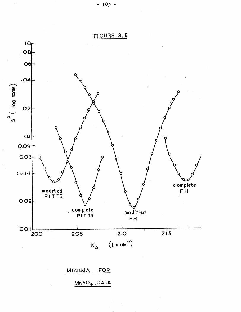
- 103 -

FIGURE 3 . 5I.Oi

0.6

0.2

O.i

0 .0 6

commodified P r T T5

FH

0.02complete

PITTS modifiedFH

0.01210

(I. mole )2 0 5200

M I N I M A FOR

MnSO^ DATA

- 10k ~

and A • This lack of sensitivity can perhaps he understood ° ±

hy considering the relatively small variation of the A / c 2slope with a (Figure 1.2) and the small change in fromextrapolation over the range a = 2-1 k R (Figure 3.3)« Theequation used to trout the high-frequency conductance datawas the complete Fuoss-Ksia equation (1.11 ) with the relaxationterms of Falkonhagen-Lcist-Kelhg added on to take account ofion atmosphere relaxation effects. The relaxation terms wereevaluated at 1 KHz (Rel.Q qq/( ) and at the frequency, f, ofmeasurement (Rel. ). This gave an equation quite sensitiveto the variations in a, K, > and A .■— 9 ii o

A = ( A - 1 \ A J ( 1 + A x /X ) / ( 1 + 3,0/2) +o eRel.0 0Q1 - Rel.f (3.21 )

In the minimisation work it has heen found useful to2consider the variation of S with two parameters in the form

of a surface. It is then possible to visualise the dependenceof S on the variations in the two parameters. Figure 3*6

2shows a 8 - K,. - a surface constructed from manganese sulphatedata using the modified Fuoss-Hsia equation with a fixed A

value of 133o09. The conditions for a minimum in this surface are then (b s2/ba a) = 0 and (bs2A A K A) A = o. A,

variation in A Q generates a scries of surfaces and application2of the condition ( 8 / ^ A A q) then leads to an overall minimum

for the data. An alternative minimisation method developed hy Justice is described in Appendix 2.

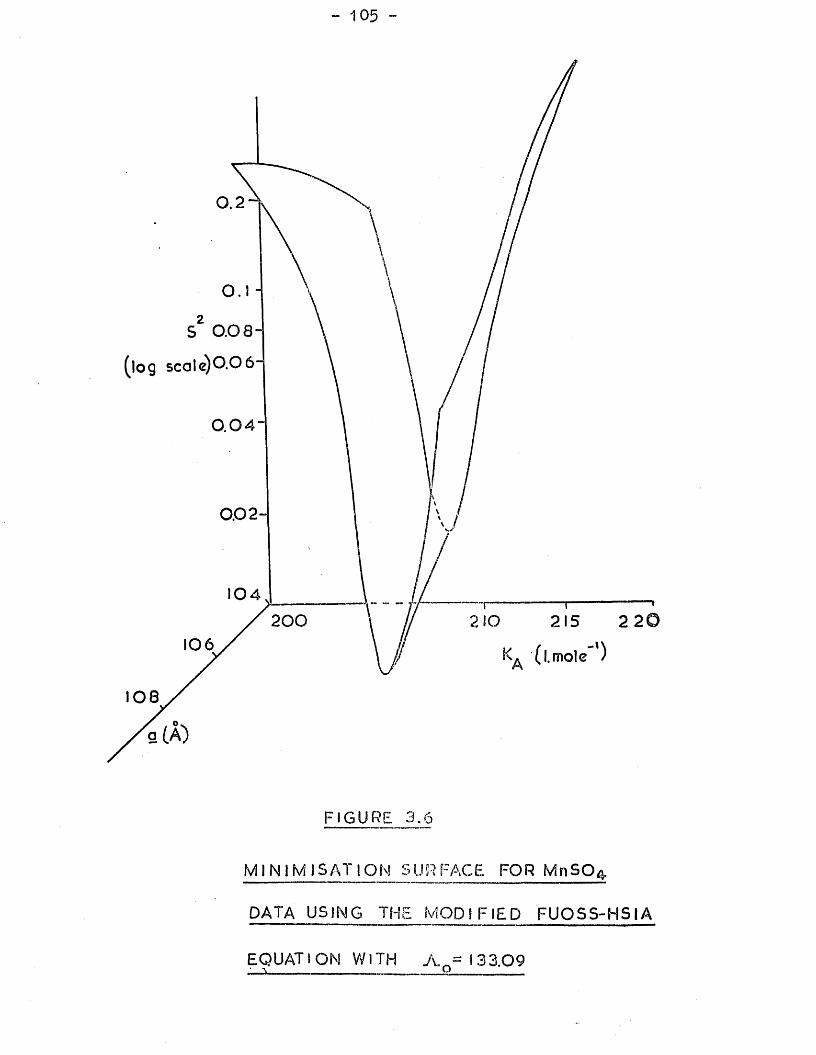
0.2

S 0 .0 8

(log s c a l e ) 0 . 0 6

O. O 4

0.02-

104

( I.mole ')

FIGURE 3.6

M IN IM IS A T IO N SURFACE FOR MnSO*

DATA USING THE M O D IF IE D FUOSS-HSIA

EQUATION WITH A = 133.09• o

EART III SECTION 2 RESULTS

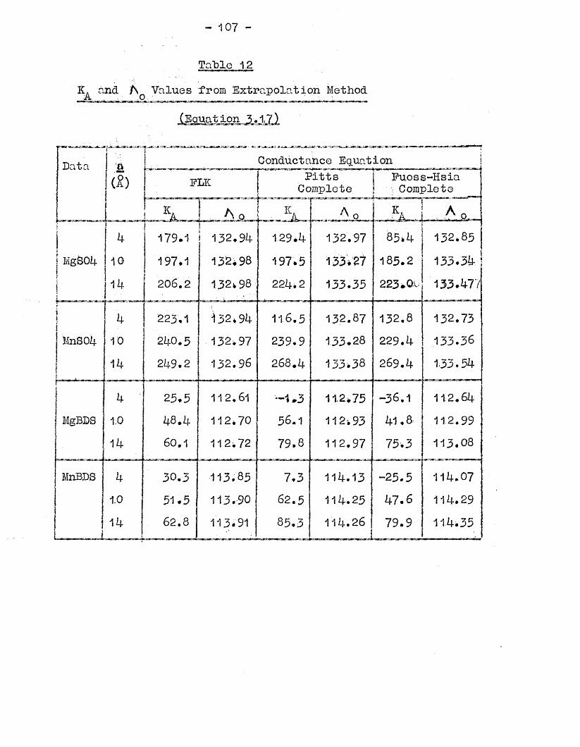
- 107 -

Table 12K. and A Values from Extrapolation Method~ A _ _ _ _ _ __ — _ _ _ _ _ __ — .

(Equation 3.1.7)

DataI

6Conductance Equation i

c£) FIK [ Pitts | Complete

| Fuoss-Hsia ! Complete

K A | A or

1 1 ,, A 0

■ h. A o

ii

i MgSOU!

i{

!

MnS04Ii!I-_ _ _ _ _ _ _ , _ _ _ _ - . . .

i

410*14

179-1'197*1206.2

132.94 132;98 132* 98

129.4197.5 224,2

132.97133.27133.35

8 5 .4

185.2223.0-

132.85133.34133.477

41014

223.1 240.5249.2

132,94132,97132.96

116.5239.9268.4

132.87133.28133,38

132.8229.4269.4

132.73133.36133.54

f IT 1

4 25.5 112.61 -1.3 112.75 -36.1 112.64MgBDS 1.0 48.4 112,70 56.1 112,93 41.8 112.99

14 60.1 112,72 79.8 112.97 75.3 113.08

MnBDS 4 30.3 113.85 7.3 114.13 -25.5 114.071.0 51.5 113.90 62.5 114.25 47.6 114.29

- - - - - - - - - -

14 62.8 113.91 85.3 114.26 79.9 114.35

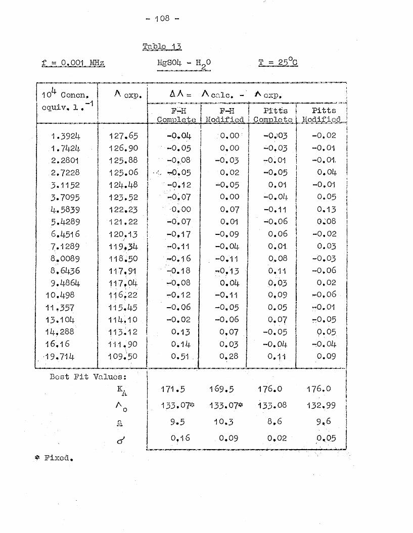
10 Concn, ] —1 !eguiv, 1.

1.3924 1.7424 2.2801

. 2.7228 3.1152 3.7095 4.5839 5.4289 6 • 4516 .7.1289 8.0089 8.6436 9.4864 10.498 11,3571 3 .1 0 414,28816.1619.714

exp,

127.65 126.90 125.88 125.06 124.48 123.52122.23 1 21.22 120.13 119.34118 .50

117,91 117.04 116 .22

115,45 114,10 113.12 111,90109.50

Best Pit Values:E/AAa

A A = A calc. - AP-H

Complete-0.Q4-0 .0 5 -0.08

• 05 - 0.12 -0.07 •0.00 -0.07-0,17 - 0.11 -0 .1 6 - 0 .18 -0.08 - 0 .1 2

- 0.06 - 0 .0 2 0.13 0 .1 4

0.51

171.5133.07*9.5 0 .1 6

P-H Modified I

exp, Pitts

169.5133.07*10.30.09

Pitts Modified

- 0.02-0J030,00-0.010,00 -0 ,0 3- 0.01-0.01

-0 .0 50.02-0.01-0 .0 5

-0 .0 40.00-0.11- 0.06

- 0.02-0 .0 9

-0 ,0 4 0 .01.-0 .0 3-0.11- 0.06-0,130.020.06- 0.11

-0.01

-0.06 r*0,05-0.05

-r0,04-0.04

1 7 6 .0

133*088,60.02

176.0 ji132,99 j9*60,05u

* Pixed.

- 109 -

Table H i.

£ = 0.001 MHz MnS04-H 0 T_=

410 Concn±, equiv. 1*

A exp. A ATm I

Complete

= A ca.

Modified

1c. - ATrltts"~

Complete

exp.“ PittsModified

1,8288 126.41 0.02 -0 .0 3 -0.08 -0.123-8173 122.69 0.03 0.05 0.03 0 .0 2 !

i

5.1959 120.65 0.01 0.06 0.06 0 .0 5

6.4233 119.07 0.00 0.06 . 0 .0 7 0 .0 7

7.4849 117.87 -0.05 0.01 0.02 0 .0 3

8.7868 11,6.52 -0.10 -0.04 -0.02 -0 .0 2.

10.236 115.07 -0.07 -0.02 0.03 0 .0 0

12.151 113.34 i. -0.03I 0.00 0.02 0.01

14.060 111.83 | -0.03 -0.04 0.00 -0 .0 4

16,241 110.22 0.03 -0.04 0.02 -0 .0 7

17.098 109.57 0.11 0.02 -0.03 -0 .0 2 j— — |

Best Fit Values:

ka 217.5 211.5 206.0 201 .5

A 0 133.25 133.09 132.98 132.95a 9.5 10.7 7.8 7.7

o ' 0.06 0.04 0.04 0.05

- 110 -

Table 15f = 0.001 MHz MgBDS-HgO Data

f| 10 Concru, j equiv. 1*1 . ■ :| ,/ / ■

ft qXv ! bh - A calc, - A. exp, |.

P-HComplete

F-H Modifi ed

PittsComplete;

PittsModifiedj

2.361+1 107.50 0.17 0 .1 6 -0.121

0.1,9 !1+. 091+5 105.91+ 0,02 0.02 -0,02 0.09 J5.961+9 101+.57 -0 .0 5 -0.03 0.02 0.067.81+39 10 3.1+3 -0,08 -0.07 0.05 0.01.8.5782 103.06 -0,12 -0.11 0.09 -0 .0 4

9.7111 102.1+1 . -0;07 ^0i06 0,01}. 0.01

11.086 101+72 -0*05 -0.03 0.02 0.01

13.152 100 ,83 -0,06 -0.05 0,0k -0 405

11+.215 100.37 -0.02 -0.01 0.01 -O.Olj.18.61+1 98.61 0,21 0 ,1 8 -0 .1 6 -0.01

Best Pit Values:

*A 50.5 3 0 .0 1+9 .0 3 0 .5

A 0 113*07 113*01 112.91 1 1 2 .9 5

a 10.5 1 1 .0 9 .0 9.70.11 0 ,0 9 0 .0 7 0 .0 7

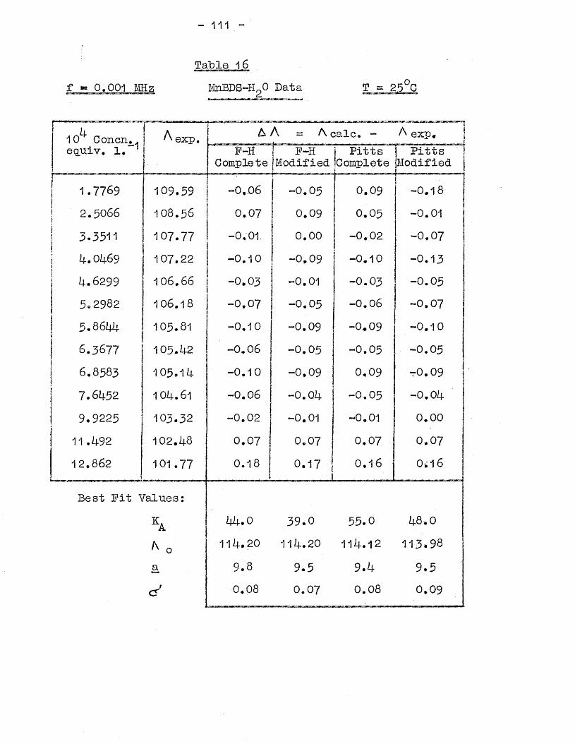
- 111 -

Tafale 16

f * 0.001 MHz MnEDS-HgO Dats

A is A = A calc. - A exp.equiv. 1. F-H | F-H I Pitts

Complete I Modified {Complete. . . - - -.. . i— . ... . iPitts

Modified

1.7769t 109.59 -0,06 -0.05 0 .0 9 -0.18f

2.5066 108,56 0.07 0 .0 9 0 ,0 3 -0.013.3511i 107.77 -0.01. 0.00 -0.02 -0.071

i i4-.oi4.69 107.22 -0.10 -0 .0 9 -0.10 -0.13u. 62991 10 6,66 -0.03 -0.01 -0 .0 3 -0.035.2982 106,18 -0 .0 7 -0 .0 5 -0.06 -0.07

| 5 .8 6 4 4E 1105.81 -0.10 -0 .0 9 -0 .0 9 -0.10

| 6 .3 67 7 105.1+2 -0.06 -0 .0 5 -0 .0 5 -0.051 6.8583 ^I j 105.11+ -0.10 -0,09 0 .0 9 T-0, 091 7.61+52 | 1 01+. 61 -0.06 -0.0 4 -0 .0 5 -0,04

9.9225 103,32 -0.02 -0.01 -0.01 0.0011.1+92 102.1+8 0 .0 7 0 .0 7 0 ,0 7 0 .0 7

12 .86 2 1 0 1 .7 7 0 .1 8 0 .1 7 0.16 0*16■ ..... I _____ -

Best Pit Values:

ka 44.0 3 9 .0 5 5 .0 48*0

^ 0 1 1 4 .2 0 114 .2 0 114 .12 113.98a 9 .8 9.5 9.4 9.5tcr 0.08 0 .0 7 0.08 0.09

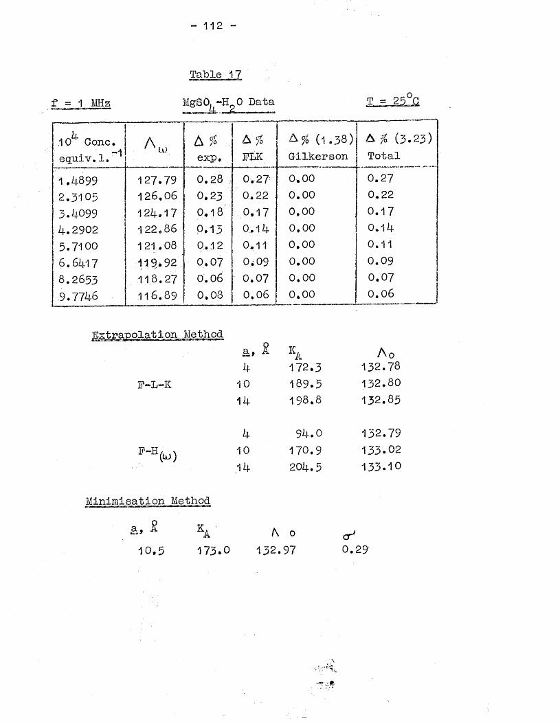
- 112 -

Table 17

f = 1 MHz MgSO. -H O Data ,T =_2_5_°CI

10 Cone. A,,

I m<3 A % (1 .3 8) A f0 (3.23)

eguiv.1. tu exp. FDK Gilkerson Total

1.4899 127.79 0.28 , 0.2? 0,00 0.272.3105 126,06 0.23 0.22 0.00 0.223.4099 124.17 0 ,1 8 .0 ,1 7 0,00 0.174.2902 122.86 0.15 0 ,1 4 0.00 0 .1 4

5.7100 121.08 0.12 0.11 0.00 0.116.6417 119>92 0,07 0i09 0.00 0.098 .2 6 5 3 118.27 0.06 0 .0 7 0,00 0.079.7746 116 .89 0,03 0 .0 6 0.00 0.06

A o132.78 132.80 132.83

132.79 133-02 133-10

<y0.29

Method

F-L-K

F-HA(w)

a,4

1014

41014

kA172.3189.5198.8

94.0170.9204.5

Minimisation Method

Ka,10.3

*A173-0

A o 132.97

- 113 -

Table 18

f = 2 MHz Data exT = 25 C

10^ Cone.• V "Iequiv.1.

A %exp.

A %FLK

A # (1 .3 8 )Gilkerson

A % (3.23)1Total

1 .5010 127 .88 0.53 0 .5 4 0 i

. 0 !

0 i

0 .5 4

2.6671 12 5 .5 8 0.43 0.47 0,00 0 .4 7

| 3.8015 123.90 0.43 0.40 0.00 0 .4 0

! 4 .6 3 8 8i 1 2 2 .7 4 0 .3 8 0 .3 6 0.00 0 .3 6

| 5.489? 121 .5 5 0.31 0 .3 2 0.00 0 .3 2

6.8012 1 2 0 .0 6 0 .3 0 0 .2 6 0.00 0 .2 6

9.0476 117.74 0.22 0.20 0.00 0 .2 0

10,1+06 116.47 0 .1 8 0 .1 7 0.00 0.1711.120 115.82 0.13 0 .1 6 0.00 0 .1 6

F-L-IC

P-H(to)

Method0a, A ka A 0

4 174.8 132.9310 192.2 132.9814 201.3 132.97

4 93.1 132.9210 173.2 133.2414 209.1 133.33

Minimisation Method

a s

1 0 .5

ka172.4

A O133.11

O0,18

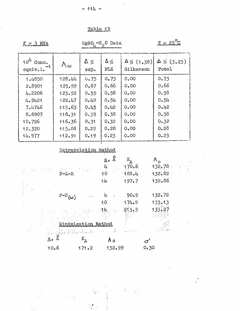
f « 5 MHz

- 112* -

Table 19

r, Ho0 Data 4 2

10 Cone.• •, “1equiv. 1. A u> A #

exp.A fa FLK

...................-

A % (1.38)G-ilkerson

A % (3.23) Total

1.4850 1 2 8 .4 4 0.75 0.73 0*00 0.732J3901 125 .59 0.67 0.66 0*00 0 .6 6 1

4 .2 20 6 1 2 3 .5 2 0.55 0.58 0*00 0 .5 8 1

4.9421 122 .47 0.49 0.54 0*00 0 .5 4 |7.4746 1 1 9 .6 3 0.45 0.42 0.00 0 .4 2 18 .6 9 0 7 118.31 0.39 0.38 0.00 0.38 |10.726 1 1 6 .3 6 0.31 0 .3 2 0,00 0*3212.320 115.08 0.29 0.28 0.00 0.28 ;14.977 112.91 0.19 0.23 0.00 .0-23

Methoda, S. ka A 04 170.6 132.78

P-Xi-K 10 188.4 1 3 2 .8 2

14 197.7 1 3 2 .8 6

P-H(W) 4 90.9 132.7210 174.9 133.13

213.5 133.27

Minimi sat i on Method

a , 1

10.6ka171.2

A o132.99

o'*0 .3 0

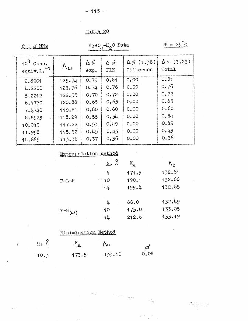
- 115 -

t = 4’ MHzm t m x i a w i iii ^ .v i f ? . *

Ta‘bl.e_jaQ

MgSO, ~H 0 Data o.T = 25 C

J+10 Cone.• -iequiv.1.

L %exp.

& %FLK

m (1 .3 8 )G-ilkerson

A /*> (p. Total

2 o 8901it. 2206 5.2212 6.14-770 7.4746 8.8923 10.049 11.958 11).. 669

125.74123.76122.35 120.88 119.81 118.29 117.22 115,32113.36

0,79 0.74 0.70 0.65 0.60 0.55 0.53 , 0.45 0.37

0.81 0.76 0.72 0.65 - 0.60 0.54 0.4-9 0.43 0 ,3 6

0 .0 00 .0 00 .0 00 .0 0

0 .0 00 .0 0

0 .0 00 .0 00 .0 0

0.810 .7 6

0 .7 2

0.650 .6 0

0.540.490.430.36

Extrapolation Methoda, ® h A 04 1 7 1 .9 132.61

F-L-K 10 190.1 132.6614 1 9 9 .4 132.65

4 8 6 .0 132.49

* " V ) 10 175.0 133.0514 212.6 133.19

Minimisation Method ■

na § r.’. ka ho d10.3 173.5 133.10 0.08

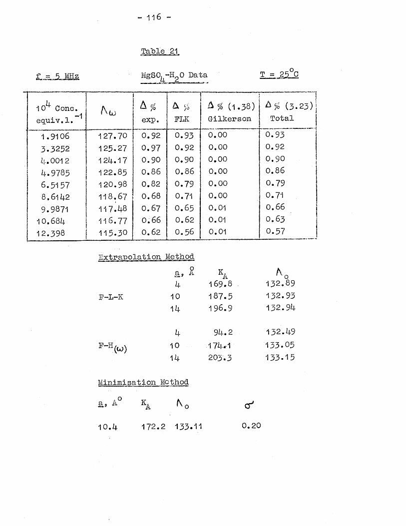
- 116 -

Table 21

f = 5 MHz McSO, -Ho0 Data T 25°C

10^ Cono.• *i -1equxv.1.

;A %exp.

A jo FLK

a % (1.3 8)G-ilkerson

(3 .2 3)Total

1.9106 1 2 7 .7 0 0.92 0.93 0.00 0.933.3252 12 5 .2 7 0 .9 7 0.92 0.00 0.924.0012 1 2 4 .1 7 0 .9 0 0.90 0.00 0.904.9785 122 .85 0 .8 6 0.86 0.00 0.866.5157 12 0 .9 8 0.82 0.79 0.00 0.798 .6142 11 8 .6 7 0.68 0.71 0.00 0.719.9871 117.48 0.67 0.63 0.01 0.6610.684 116.77 0.66 0 .6 2 0.01 0.6312.398 115.30 0.62

..... -..... -O.56 0.01 0.57

Extrapo! 1 Methoda, S. ka N 0A 1 6 9 .8 1 3 2 .8 9

F-L-K 10 1 8 7 .5 1 3 2 .9 3

1A 19 6 .9 1 3 2 .9 4

A 94.2 1 3 2 .4 9

F" V ) 10 ■ 174*1 1 3 3 .0 5

1A 203.3 1 3 3 .1 5

Minimisation Me thod

■\° a, A ka N o cr11 0.A 1 7 2.2 133.11 0 .2 0

- 117 -

Table 22

f = 10 MHz MgSO^-HgO Data T = 25 C

10 Cone.• -1 equxv.1.

K A %

MR<3

&,-■> (1 .3 8) (3 .2 3)to exp. FLK G-ilkerson Total

2.4271 127 .0 5 1.18 1 .22 0.00 1.222.8205 126 .4 9 1.28 1 .24 0.01 1 ,253*5443 1 2 5 .2 4 1.30 1 ,28 0.01 1.294.2662 1 2 4 .3 4 1.30 1 .31 0.01 1 ,32

5.4912 1 2 2 .7 9 1.33 1.33 0.01 1 .346 .8 11 5 121 .29 1.33 1.33 0.01 1.348.0007 120.06 1.32 1.31 0.02 1.338 ,6 81 0 119.31 1.28 1.29 0.02 1.3110.040 118.04 1.25 1.24 0.02 1 .2 6

11.821 116.45 1.20.........—

1.19 —

0.02 1 .21

Extrapolation Method

F-L-K

F-H(<*>)

a, S. ka ' Ao4 1 7 2 .4 13 2 .7 8

10 1 9 0 .2 13 2 .8 2

14 199.7 1 3 2 .8 2

4 93.3 1 3 2 .7 4

10 175.1 133.11

14 210.7 1 3 3 .2 2

Minimisation Method

9 A o10.5 174*0 133.09

ci 0.18

i

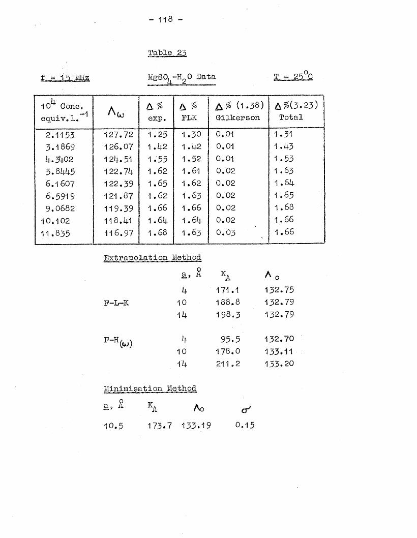
- 118 -

MgSO^-HgO Data

10 Cone, equiv.l. Ato A. %

exp.A %FLK

A % ("I *38) G-ilkerson

A^(3.23)Total

2.1153 1 2 7 .7 2 1.25 1 .30 0.01 1.313.1869 126 .07 1 .42 1 .42 0,01 1.434.3402 1 2k. 51 1.55 1.52 0.01 1.535.8445 122.74 1 .6 2 1.61 0.02 1 .6 3

6,1607 122.39 1 .6 5 1.62 0.02 1.646.5919 121.87 1.62 1 .63 0.02 1.659.0682 119.39 1.66 1.66 0.02 1.6810.102 118.41 1 .6 4 1 .6 4 0.02 1.6611.635 116.97 1.68 1 .6 3 0.03 1.66

Extrapolation Methoda, £ ka ^ 0

4 171.1 132.73F - I r - K 10 188.8 132.79

14 198.3 132.79

4 93.3 132.7010 178.0 133.1114 211.2 133.20

Minimisation Method

° kA Ao o '

1 0 .5 173*7 133.19 0 .1 5

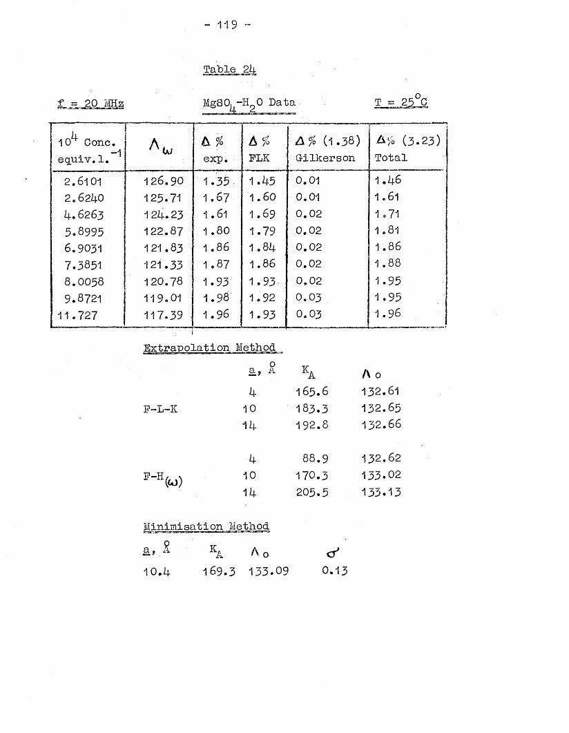
- 119

Table 2U

20 MHz MgS0^-H90 Data

10 Cone.• n “1equiv.1.

3< A S& exp.

■ & % PLK

A % (1.38)G-ilkerson

;

(3.23)Total

2.6101 1 2 6 .9 0 1.35 1.45 0.01 1 .4 6

2.6240 125.71 1.67 1 .6 0 0.01 1.61

4. 6263 124 .2 3 1.61 1 .6 9 0.02 1 *715.8995 122.87 1.80 1.79 0.02 1.816.9031 121.83 1.86 1.84 0.02 1.867.3851 121.33 1.87 1.86 0.02 1.888 .OO58 120.78 1.93 1.93 0.02 1.959.8721 119.01 1.98 1.92 0,03 1.9511.727 117.39 1.96 1.93 0 .0 3 1.96

a, A ka A 04 16 5 .6 132.61

F-L-K 10 18 3 .3 1 3 2 .6 519 2 .8 1 3 2 .6 6

4 8 8 .9 13 2 .6 2

10 170 .3 133.0214 2 0 5 .5 133.13

Minimisation Method9a, A 0<w

10.4 1 6 9 .3 1 3 3 .0 9 0 .1 3

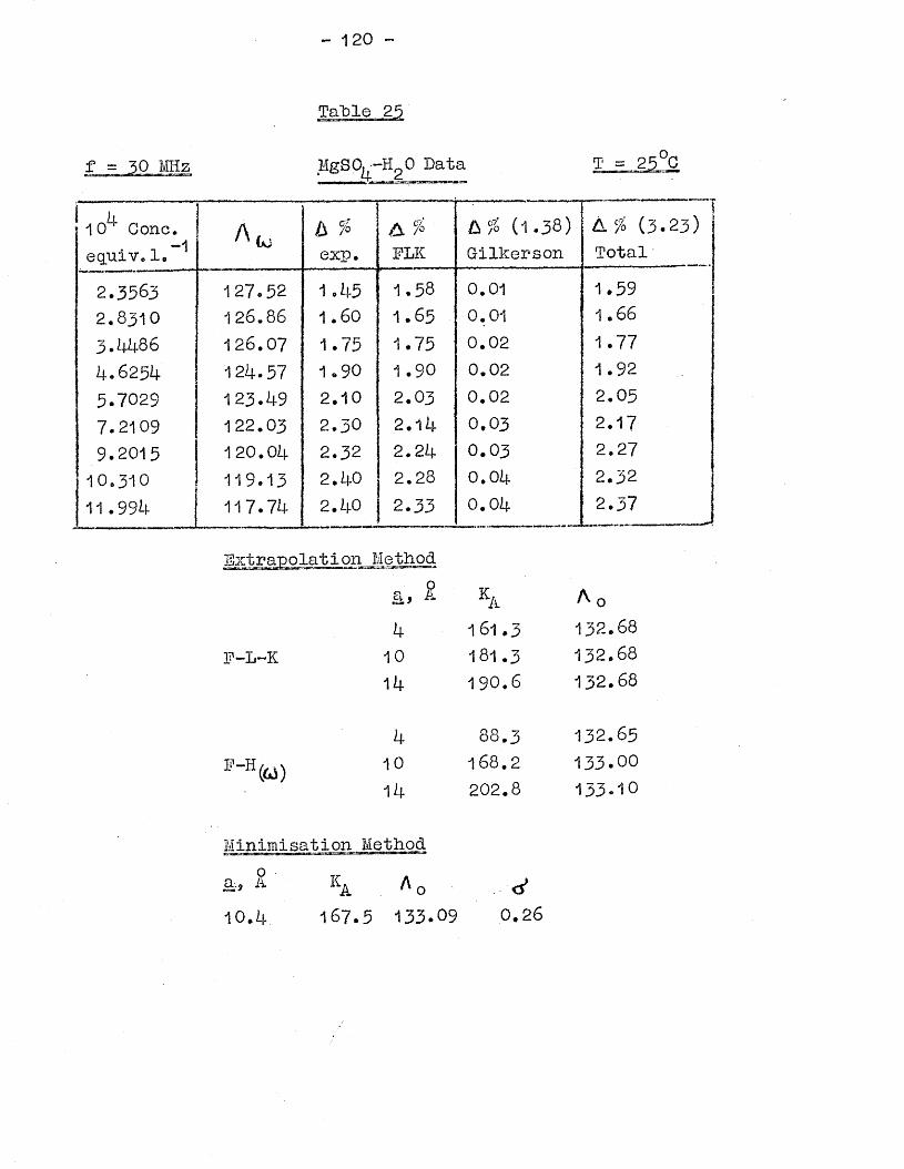
- 120 -

MgSO^-HgO Data o,T = 25 C

10 Cone, -1equiv. 1.

h % exp.

a %ELK

L % (1-38) Oillierson

A. % (3-23Total

2.3563 127.52 1.45 1.58 0.01 1.592.8310 126 .86 1.60 1 .6 5 0.01 1.663.4486 126.07 1.75 1.75 0.02 1.774.6254 124.57 1.90 1 .9 0 0.02 1.925.7029 123.49 2.10 2.03 0.02 2.057.21 09 122.03 2.30 2.14 0.03 2.179.2013 120.04 2.32 2.24 0.03 2.2710.310 119.13 2.40 2.28 0.04 2 .3 2

11.994 117.74 2.40 2.33 0 .0 4 2.37

Extrapolation Methoda, £ ka A 04 1 6 1 .3 132.68

F-L-K 10 18 1 .3 132.6814 190.6 1 3 2.68

4 8 8 .3 132.65F-H(0) 10 1 6 8 .2 133.00

14 202.8 133.10

Minimisation Methoda., 0<< o'10.4 1 6 7 .5 13 3 .0 9 0 .2 6

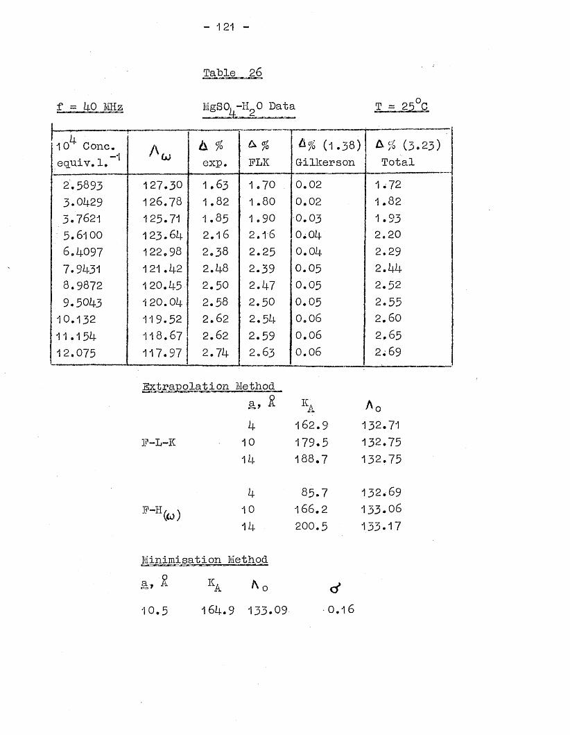
- 121 -

Table 26

f = 40 MHz MgSO^-HgO Data T = 25°C

i_L10 Cone,. n -1equiv. 1*

r..— -- —

A *b %exp.

& % FLK

(1.38)Gillierson

(3 .2 3)Total

2'. 5893 127.30 1 .6 3 1.70 0.02 1.723.0429 126.78 1 .8 2 1 .80 0.02 1.823.7621 125.71 1.85 1.90 0.03 1.935.6100 123.64 2 .1 6 2 .1 6 0.04 2.206. 4097 122.98 2.38 2.25 0.01+ 2.297.9431 121.42 2.48 2.39 0.03 2.448.9872 120.45 2.50 2.47 0.05 2.529.5043 120.04 2.58 2.50 0.03 2.55

10 .132 119.52 2 .6 2 2.54 0.06 2.6011.154 118.67 2.62 2.59 0.06 2.6512.075 117.97 2.74 2 .6 3 0.06 2; 69

Extrapolation Method>a 4 jx ^ r t ^ s a u s J rg « T : .w « .‘ .a c a « .«ajt? i»r.,j< 1 j i>w«j-smag* s«Bg«»e.‘Ba»

a, Sk

E-L-K 1011+

k1014

ka A 0162.9 132.71179.5 132.75188.7 132.75

85.7 1 3 2 .6 91 6 6 .2 133-06200.5 133.17

Minimisation Methoda, -2 Ka * q ^

10.5 164.9 133.09 0 .1 6

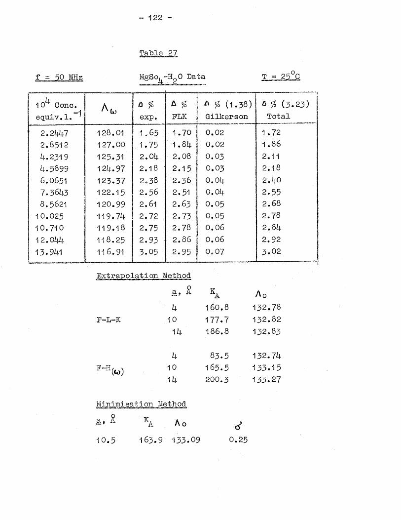
- 122 -

f = 50 MHz MgSo^-HgO Data

10 Cone.-Aequiv.1.

3 <

|

a %exp.

A %ELK

A % (1.38) Gilkerson

— 1 ----—ja % (3 .2 3)Total

2.21*7 128.01 1.65 1.70 0.02 1.722.8512 127.00 .1.75 1 • 84 0.02 1.864.2319 125.31 2.04 2.08 0 .0 3 2.114.5899 124.97 2 .1 8 2.15 0 .0 3 2 .1 8

6.O651 123.37 2 .3 8 2.36 0.04 2.407.3643 122.15 2 .5 6 2.51 0.04 2.558.5621 120.99 2.61 2.63 0.05 2.6810.025 119.74 2.72 2.73 0.05 2.7810.710 119.18 2.75 2.7 8 0.06 2.8412.044 118.25 2.93 2.86 0.06 2.9213.941 116.91 3.05 2.95 0.07 3.02

Extrapolation Methoda, R KA A 04 1 60,8 132.78

F-L-K 10 177.7 132.8214 186.8 132 .83

4 83.5 132.74F"H(«0) 1° 165.5 133.15

14 200.3 133.27

Mjjjlmisation Method

— 9 ^ Ao10.5 16 3 .9 133.09 0.25

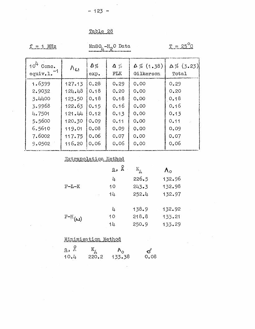
Table 28

f = 1 MHz MnSO, ~Ho0 Data k 2o.T = 25 C

IcA Cone.■ •, -1 equiv.l.

. 11. _ii ».

A w

,

exp.Ck /i> PLK

r... ~& % (1 .3 8)Gilkerson

b-% (3.2 Total

1 .6 3 9 9 12 7 .1 3 C.28 0.29 0.00 0.292 .9 03 2 124.48 0 .1 8 0.20 0.00 0.203.41+00 123.50 0 .1 8 0.18 0.00 . 0 .1 83.9968 122.63 0.15 0 .1 6 0.00 0.1 64.7501 1 2 1.44 0.12 0 .1 3 0.00 O.135 .5600 120 .3 0 0.09 0.11 0.00 O.11

6 .5610 119.01 0.08 0 .0 9 0.00 0.097.6002 117.75 0.06 0 .0 7 0.00 0.079.0502 116 .20 0 .0 6 0.06 0.00 0.06

Extrapolation Methoda, 2. ka Aok 226* 3 13 2 .9 6

P-L-K 10 2 if-3-3 132 .98252.if. 13 2 .9 7

k 138.9 13 2 .9 2

F"?(W) 10 218,8 133.21

1i+ 250.9 1 3 3 .2 9

Minimisation Method

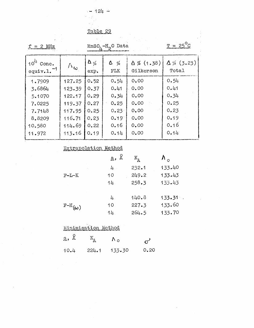
4 ~.

10^ Cone.-1equiv.1.

r. .....

■ V& </0exp.

■ & % FLK

A % (1 .3 8)Gilkerson

ij A % (3 .2 3)! Total

1.7909 127 .25 0.52 0.54 0.00 0.543 .6864 12 3 .3 9 0.37 0.41 0.00 0.415.1070 122 .17 0.29 0.34 0.00 0.347.0225 11 9 .3 7 0.27 0.25 0.00 0.257.7148 1 1 7 .9 5 0.25 0.23 0.00 0.238.8209 116.71 0.23 0.19 0.00 0 .1 910.580 1 1 4 .6 9 0.22 0 .1 6 0.00 0 .1 6

11.9721

113 .1 6 0.19 0.14 0.00 0 .1 4

Method a, 2.4

P-L-K 10

14

ka232.1

2 4 9 .2

2 5 8 .3

A 013 3 .4 0

1 3 3 .4 3

1 3 3 .4 3

P-H(w)4

10

14

1 4 0 .8

2 2 7 .32 6 4 .5

133.311 3 3 .60133.70

Minimisation Method

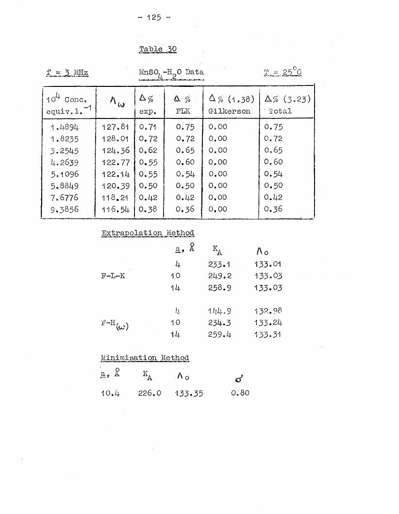
- 125 -

Table 30

f = 3.. MHz MnSO, -H_0 Data T - 25°C

ICr Cone.n “Iequiv. 1«

I

exp.A. % •ELK

(1.38)G-ilkerson

A-$ (3 .2 3)'Total

1 .4894 ’127.81 0.71 0.75 0.00 0.751.8235 128.01 0.72 0.72 0.00 0.723•2545 12 4 .36 0.62 0 .6 5 0.00 0.654.2639 122.77 0.55 0.60 0.00 0. 603 d 096 122.14 0.55 0.54 0.00 0 .5 4

5,8849 120,39 0.50 0 .5 0 0.00 0 .5 0

7.6776 118.21 0.42 0.42 0.00 0.!+29 .3 8 5 6 1 1 6.54 O.38 0 .3 6 0.00 O.3 6

Extrapolation Methoda, $ ka A 04 233.1 133.01

F-L-K 10 2 4 9 .2 133 .03

14 2 5 8 .9 133 .0 3

4 144-9 132 .9810 234.3 1 3 3 .2 4

14 259.4 133.31

jlinimi sat i on Methoda, £ Ka A 010.4 226.0 1 3 3 .3 5 0.80

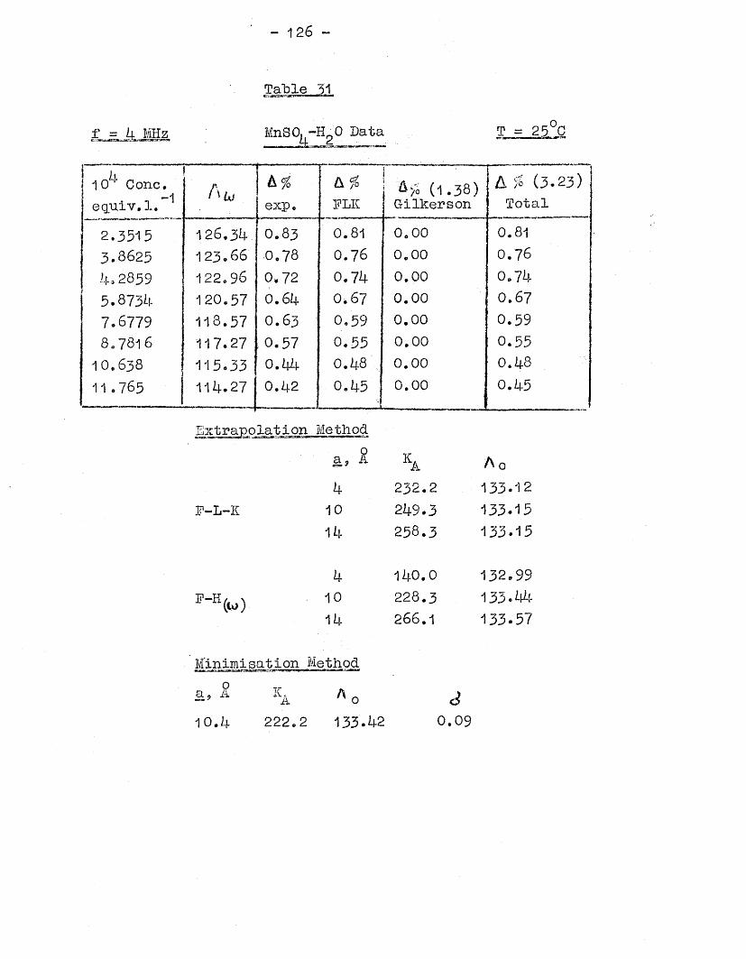
- 126 ~

MnSO, -HUO Data

; 10 * Cone.. . -1 equiv. 1. /'Ui

&%exp.

r n-.tr t ,

ts.%FLIC

(1.38)Gilkerson

■ 'A $ (3 .2 3)Total

2.3515 1 2 6 .3 4 0.83 0.81 0.00 0.813.3625 1 2 3 .6 6 0.78 0.76 0.00 0.764.2859 122 .96 0,72 0.74 0.00 0.745.8734 1 2 0 .5 7 0.64 0.67 0.00 0.677.6779 11 8 .5 7 O .63 0.59 0.00 0.598 .7 81 6 117.27 0.57 0.55 0,00 0.55

1 0 .638 115.33 0.44 0.48 0.00 0.481 1 .7 6 5 | 114.27 0.42 0.45

- .. ................i0.00 0.45

Extrapolation Method

F-L-K

a .

410

14

2 3 2 .2

249 .3

25 8 .3

A o133.12133.15133-15

F-H(hi)4

10

14

140.02 2 8 .3

266.1

1 3 2 .9 91 3 3 .4 41 3 3 .5 7

Minimisation Methoda, A1 0 .4

A,A222.2 133 .42

30 .0 9

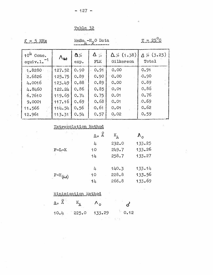
- 127 -

*LjlJLJS2 MnSo.-■H O Data T-Jg.-

10^ Cone.-1equiv.l. ! I I

>

i I

i ..

0l%exp.

A ;oFLIC

A.^ (1 .5 8) G-ilkerson

A #Tot

1.8280 127 .52 0,90 • 0.91 0.00 0.912.6826 125 .7 5 0.89 0 ,9 0 0 .0 0 •0 .9 0

4 .0 01 6 123.4? 0.88 0.89 0.00 0.894 .846O 122.24 0.86 0,85 0.01 0.866.7610 119.85 0,74 0.75 0.01 0.769.0001 117.18 0.69 0.88 0,01 0.69

11.566 114.54 0.56 0.61 0.01 0.6212.961 113.31 0.54 0.57 0, 02 0,59

F-L-K

F-H(CO)

a4

10

14

41014

KA23 2 .0

249.7258.7

140.3228.8 2 6 6 .8

*013 3 .2 51 3 3 .2 6

13 3 .2 7

1 3 3 .1 41 3 3 .5 6

1 3 3 .6 9

Minimisation Methoda, £

10.4

K, AA '' o225.O 133.29 0 .1 2

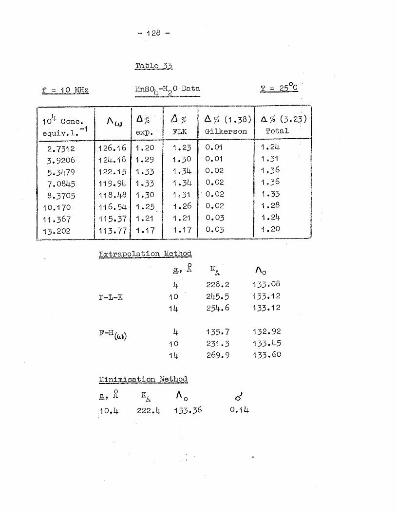
128 -

Ta~ble 35

f = 10 MHz MnSO^-H^O Data

10^ Cone.-1equiv.l.

Ac.exp.

/s %PLK

& % (1.38) G-ilkerson

Cl % (3 .2 5)Total

2.7312 .126.16 1 .2 0 1.23 0.01 1.2k3 .9 2 0 6 124.18 1 .29 1 .30 0.01 1 .315 .3479 122.15 1.33 1.3*4- 0.02 1 .3 6

7.0845 119.94 1.33 1.3k 0.02 1 .3 6

8.3705 118.48 1.30 1.31 0.02 1 .3 3

10.170 116.54 1.25 1 .2 6 0.02 1 .2 8

11.367 115.37 1.21 1.21 . 0.03 1 .2 4

13.202 113.77 1.17 1.17 0.03 1 .2 0

Extrapolation Methodci. g X-i.

F-L-K41014

ka228.2245.5254.6

A 0133.08133.12133.12

F-H(<d) 41014

135.7231.3269.9

132.92133.45133.60

Minimisation Method a, S.1 0 *2+ 2 2 2 .4

' o133 .36

<s>0 .1 4

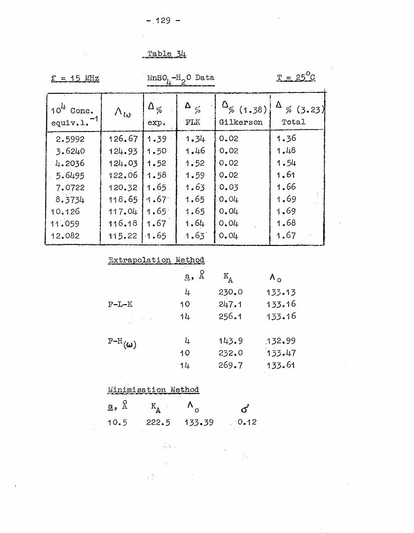
-.129 -

MnSO, -Ho0 Data

10 Cone.-1equiv.1.

^ to

<3 A %&% (1 .3 8) A $ (3.23)

exp. PLK G-ilkerson Total2 .5992 1 2 6 .6 7 1.39 1.34 0.02 1 .3 6

3.6240 121+. 93 1.50 1 *46 0.02 1.1+8

4.2036 121+.03 1.32 ■1.52 0.02 1.51+5.6495 122.06 1.58 1.59 0.02 1.61

7.0722 120.32 1 ♦ 65 1 .6 3 0 .0 3 1.668.3734 118.65 ‘1.67" 1.65 0.01+ 1.6910.126 117.01+ 1.6 5 ; 1 .6 5 0.01+ 1.691 1.059 11 6 .1 8 1.67 1.6 4 0.01+ 1.6812.082 | 115.22 ■1 .6 5 1 .63: 0.01+ 1.67

a, S.4

F-L-K 1014

F~ V ) *1014

Minimi sa t i on Methoda„ S ka A

10.5 222.5

230.0 133.1321+7.1 133.16256.1 133.16

11+3.9 132 .99232.0 153.1+7269.7 133.61

o133.39 -0.12

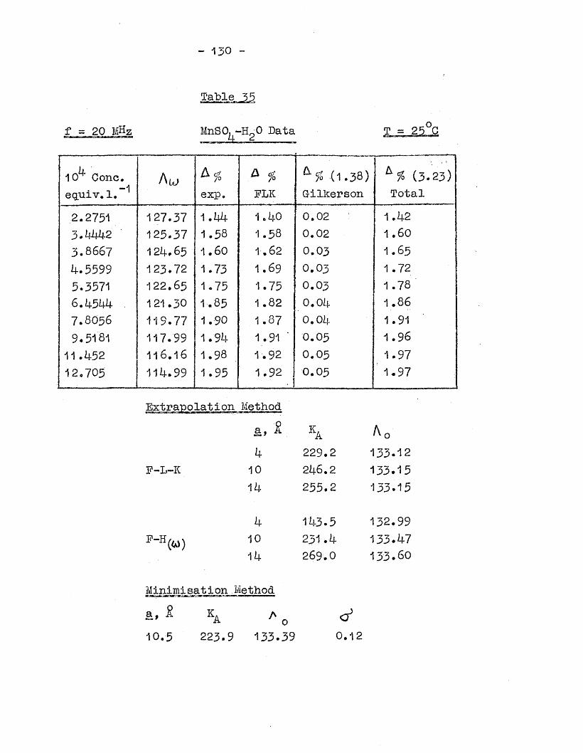
- 130 -

MnSO, ~Ho0 Bata

10 Cone, -1equiv.1,

A $exp.

& %FLK

(1,38)Bilkerson

(3.23)Total

2.2751 127.37 1.44 1.40 0.02 1 .423.4442 125-37 1.58 1.58 0.02 1.603.8667 124.65 1.60 -I .62 0.03 1 • 65

4.5599 123.72 1.73 1 .69 0 .0 3 1.725.3571 122.65 1.75 1.75 0.03 1.786.4544 121 .30 1 .8 5 1 .82 0.04 1.867 .8 05 6 119.77 1.90 1.87 0.04 1.919.5181 117.99 1.94 1.91 ' 0.05 1.96

11.452 116 .16 1.98 1.92 0.05 1.9712.705 114.99 1.95 1.92 0.05 1.97

Extrapolation Method

4F-L-K 10

14

4F-H (W) 10

14

Minimisation Method

ka Ac229 .2 1 3 3 .1 2

246.2 1 3 3 .1 52 5 5 .2 13 3 .1 5

143*5 13 2 .9 9

231.4 133.47269.0 1 3 3 .6 0

<7*a, * Ka a o10.5 223.9 133.39 0.12

- 131 -

Table 36

MnSO, -H_ 0 Data

10 Cone, eguiv.1. exp.

4 % PLK

& % (1 .3 8)Gilkerson

& fo (3.23) Total

2.5^62 1 2 7 .0 0 1.61 1.55 0.04 1.593.3052 125 .5 8 1.60 1,69 0.03 1.7!+!+. 1606 12!+. 33 1.70 1.80 0.06 1.86!+.8W+ 123.68 2.00 1.90 0 ,0 6 1.966 .1 3 0 7 122.01 2.06 2 .0 4 0.07 2.118 .2099 119.83 2.34 2.17 0.09 2 .2 6

10 .38 5 117.56 2 .3 2 2 .2 6 0 .1 0 2.3611 .67 2 116.5!+ 2.50 2 .3 0 0.11 2.1+113 .560 115.07 2.60 2.37 0.12 2.!+9

StijZu j?9/pOlation Methoda, R ka A 04 21 5 .5 1 3 3 .1 2

F-L-K 10 23 2 .5 13 3 .1 5

14 21+1.!+ 133.15

4 131.6 132.92

10 219.1 133.!+514 256.3 133-5U

Minimisation Methoda, R 1 :KA •Ao1 0 .6 211+.0 133.40 0.62

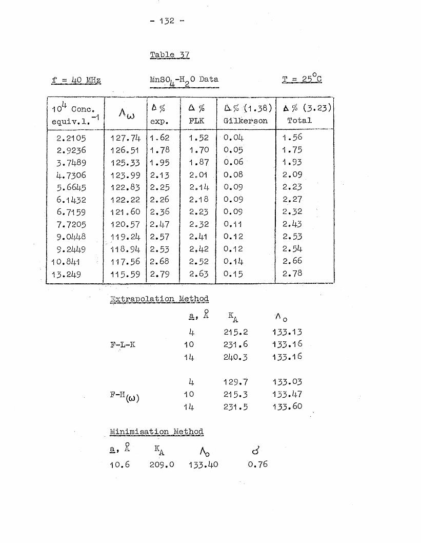
- 132 -

MnSOi-BLO Data

* 4 10 Conco-1equiv.1.

3 ;

< 4 %exp.

A f0 FLK

(1 .3 8)G-ilkerson

(3.23)Total

2.2105 127.74 1 ,62 1 .52 0 .0 4 1 .5 6

2.9236 126.51 1 .78 1.70 0.05 1 .7 5

3.7489 125.33 1 .95 1 .87 0 .0 6 1 .9 34.7306 123.99 2.13 2 c 01 0 .0 8 2 .0 9

5.6645 122 .83 2.25 2„1k 0.09 2 .2 3

6.1432 1 2 2 .2 2 2 .2 6 2 .1 8 0.09 2 .2 7

6.7159 1 2 1 .6 0 2 ,3 6 2.23 0.09 2 .3 27.7205 120.57 2. k7 2.32 0.11 2 .4 3

9.0448 119.24 2.57 2.U1 0.12 2 .5 3

9.2449 118.94 2.53 2.42 0.12 2 .5 4

10.841 117.56 2.68 2.52 0.14 2.6613.249 115.59 2.79 2.63 0.15 2.78

F-L-K

a4

10

14

ka215.2231.6240.3

^ o133.13133.16133.16

F-H(W)41014

129.7215.3231.5

133-03133.47133.60

Minimisation Methoda, £ 10.6 209.0

A<>133.40 0.76

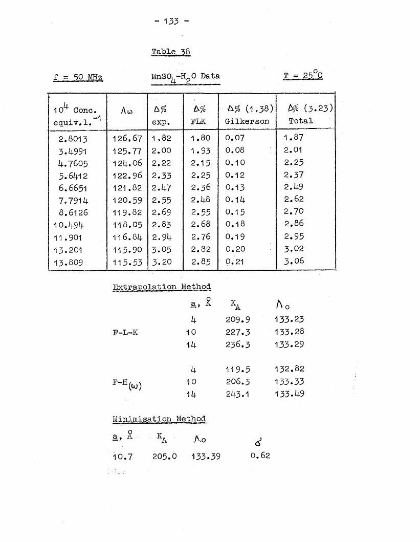
Table 38

MnSO r-HgO Data

10 Cone.--iequiv.1.Aw

exp.bs.%FLK

■h% (1.38) Gilkerson

Mi (3 .2 3)Total

2.8013 126.67 1 .82 1.80 0.07 1.873*4991 125.77 2.00 1.93 0,08 2.014.7605 124.06 2.22 2.15 0 .1 0 2.255.6412 122.96 2.33 2.25 0.12 2.376.6651 121.82 2.47 2 .3 6 0,13 2.497.7914 120.59 2.55 2.48 0 .1 4 2 .6 2

8.6126 119.82 2.69 2.55 0.15 2.7010.494 1 1 8 .0 5 2 .83 2.68 0 .1 8 2.8611.901 116.84 2.94 2.76 0.19 2.9513.201 115.90 3.05 2.82 0.20 3.0213.809 115.53 3.20 2.85 0.21 3.06

Extrapolation Method

F-L-K

p-H(W)

a, S. ka A o4 20 9 .9 1 3 3 .2 310 22 7 .3 1 3 3 .2 8

14 23 6 .3 1 3 3 .2 9

4 1 1 9 .5 1 3 2 .8 2

10 206.3 13 3 .3 3

14 243.1 1 3 3 .4 9

Minimisation Method

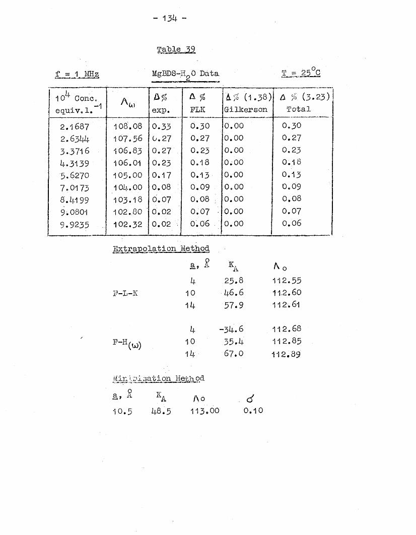
- 134 -

f = 1 MHz MgBDS-HgO Data. T = 25 C

10^ Cone..

<l r “ - - ...(1 .3 8) A % (3 .2 3

—jequiv. 1. exp. FLIC Gilkerson Total2.1687 108.08 0.33 O.3O 0.00 0.302.631+1+ 107.56 0.27 0.27 0.00 0.273.3716 106.83 0.27 0.23 0.00 0.231+.3139 106.01 0.23 0.18 0

0

' *0 0.185.6270 105.00 0.17 0.13 0.00 0.137.0173 101+. 00 0.08 0.09 0 .00 0.098.1+199 103.18 o'. 07 0.08 0 .0 0 0.089.0801 102.80 0.02 0.07 • 0 .00 0.079.9235 102.32 0 .02 •

.j0.06 0 .00 0.06

Extrapolation Method

F-L-K

■F-H(u)

a, A A ^ o4 25.8 112.5510 4 6.6 112.6014 57.9 112.61

4 -34.6 11 2.6810 35.4 112.8514 67.0 112.89

Min I d.1 sat ion Method

^ l\ o10.5 1+8.5 113.00

d0.10

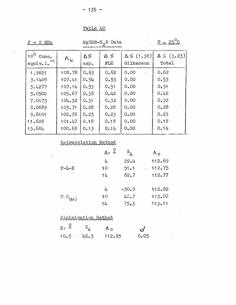
- 135 -

£ = 2 MHz

Table 40

MgBDS-HgO Data T

Extrapolation Methoda, 2.

F-L-K41014

ka 29.4 51.1 62.7

10 Cone, equiv. 1. A<o exp.

A % FLK

:

(1.38)Gdlkerson

6 % (3.23) Total

1 .9621 1 0 8 .7 8 0 .6 3 0 .6 2 0 .0 0 0 .6 2

3.1409 107.41 0.54, 0 .5 3 0.00 0.533.4277 107.1*1 0.53 0-. 51 0.00 0.515 .0502 105.67 0.38. 0.42 0.00 0.427.0173 104.32 0.31 0.32 0.00 0.328.0689 103.71 0.28 0 .2 8 0.00 0.289.6101 102.78 0.23 0.23 0.00 0.23

11.628 101.47 0 .1 8 0.1.8 0.00 0.1813.684 100.69 0 .1 3 0.14 0.00 0.14

A o112.69112.75112.77

F--H41014

-3 0.9 42.7 15*3

112.82113.06113.11

Minimi sation Method a ? 2 K10.5 46.3

A 0112.95

O*0 .0 5

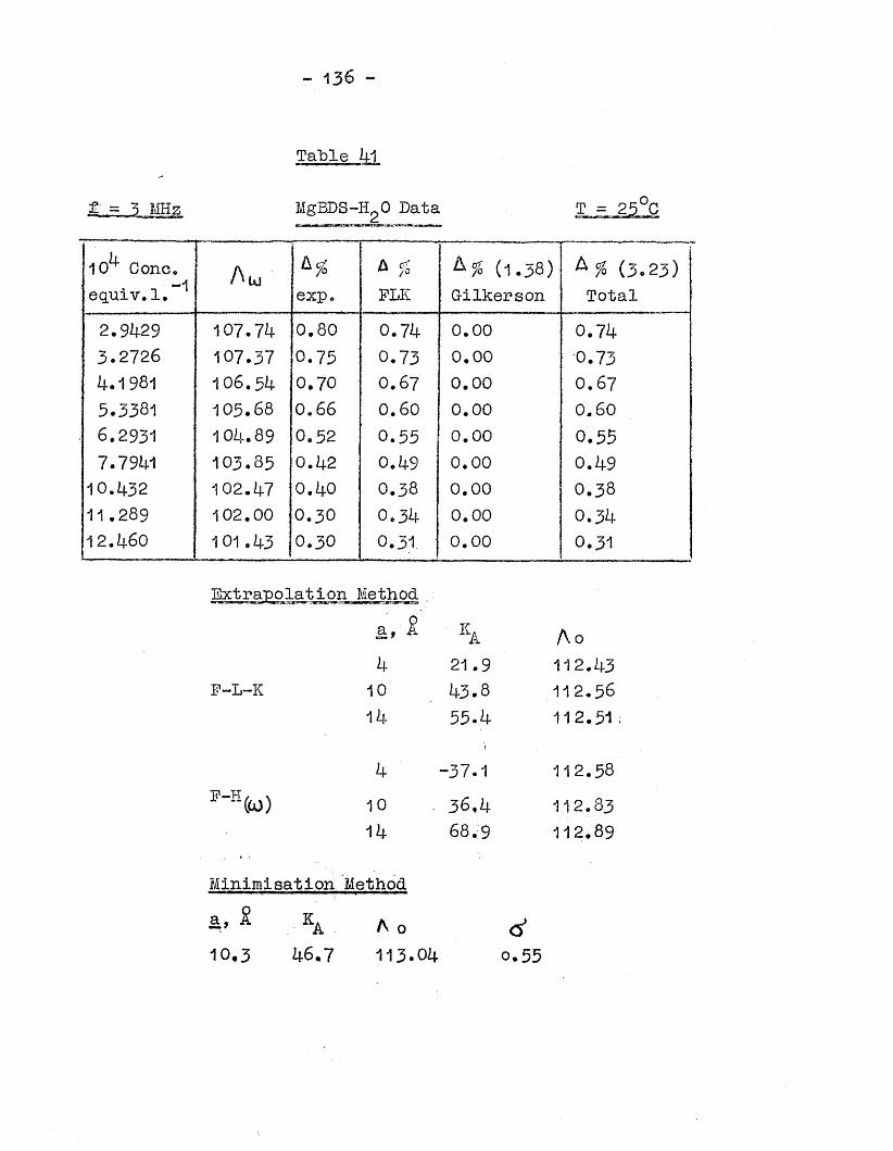
- 136 ~

Table 41m=*mesa^pcMcat ,m r a-iwi ■

& - 3 MHz MgEDS-HgO Data T = 25°C

10A Cone.• -i -1equiv.1. Am exp.

A JS FLK

(1.3 8)Gilkerson

A % (3 .2 3)Total

2.9429 107.74 0.80 0.74 0.00 0 .7 43.2726 107.37 0.75 0.73 0.00 0 .7 34.1981 106.54 0.70 0.67 0.00 0 .6 75.3381 105.68 0.66 0.60 0.00 0.606.2931 104.89 O.5 2 0.55 0.00 0.557.7941 103.85 0.42 0.49 0.00 0.4910.432 102.47 0.40 0 .3 8 0.00 0 .3 811.289 102.00 0 .3 0 0.34 0.00 0.3412.460 101.43 0 .3 0 0.31 0.00 O.31

Extrapolation Methoda ,

4P-L-K 10

14

F“H(a)) 10

14

Minimisation Method

10,3 46,7 113.

ka Ao21.9 112.4343.8 1 1 2 .5 6

55.4 112.51

-37.1 112 .58

36.4 112 .83

68.9 112 .89

<5*o,55

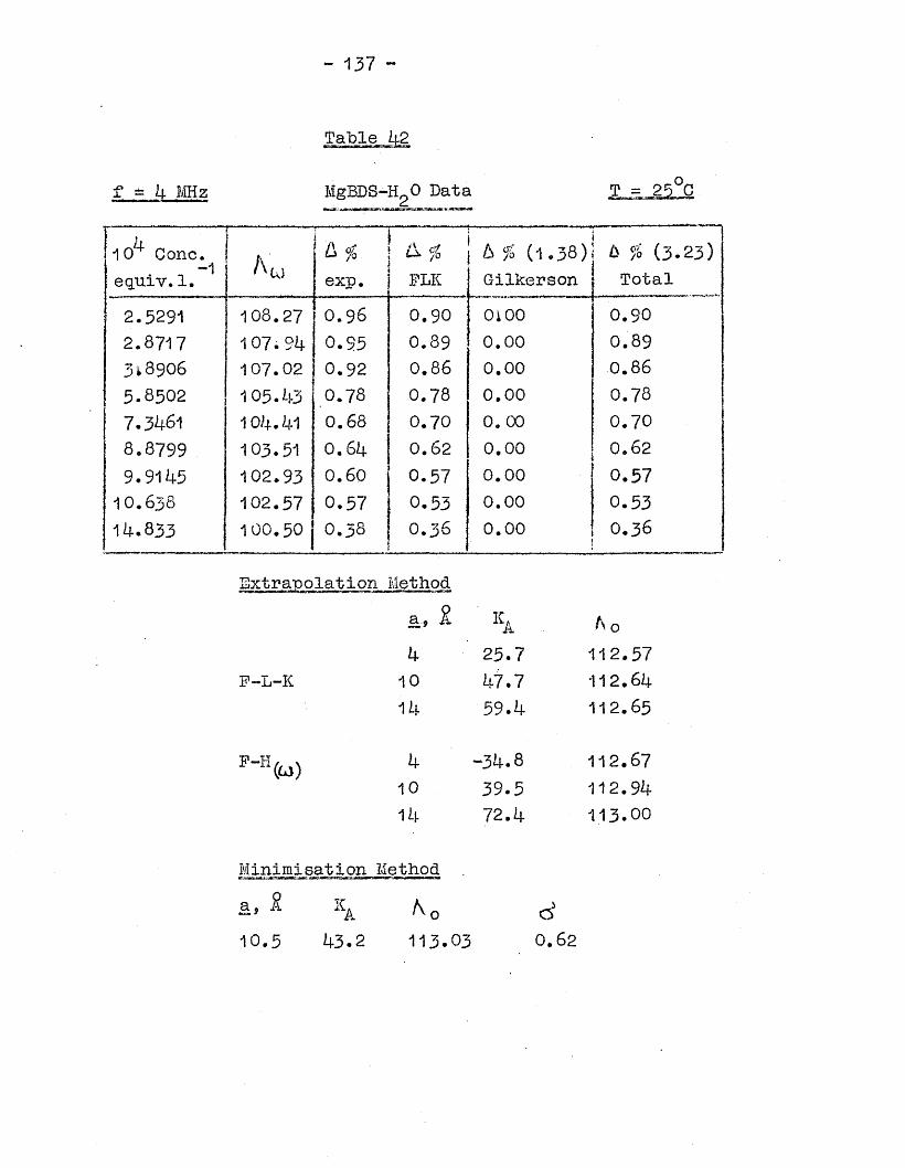
Table 42

f = 4 MHz MgBDS-H.O Data T = 25°C

Cone.. . -1 equiv.1.

-----.—& fo exp.

faFLIC

A % (1.38) Gilkerson

4 % (3.23) Total

2.5291 108.27 0.96 0.90 OiOO 0 .9 0

2.8717 107.94 0.95 0.89 0.00 0.893i8906 107.02 0.92 0.86 0.00 0.865.8502 105.43 0.78 0.78 0.00 0.787.3461 104.41 0.68 0.70 0.00 0.708.8799 103.51 0 .6 4 0 .6 2 0.00 0.629.9145 102.93 0.60 0.57 0.00 0.57■\ 0 .6 38 102.57 0.57 : 0.53 0.00 0.5314.833 100.50 0 .3 8 O.3 6 0.00

.0 .3 6

F-L-Ii

F-H(U)

Method a, £ ka t\ 04 2 5 .7 112.57

10 47.7 112.6414 59.4 112.65

4 -34.8 112.6710 39.5 112.9414 72.4 1 1 3 .0 0

Minimisation Method

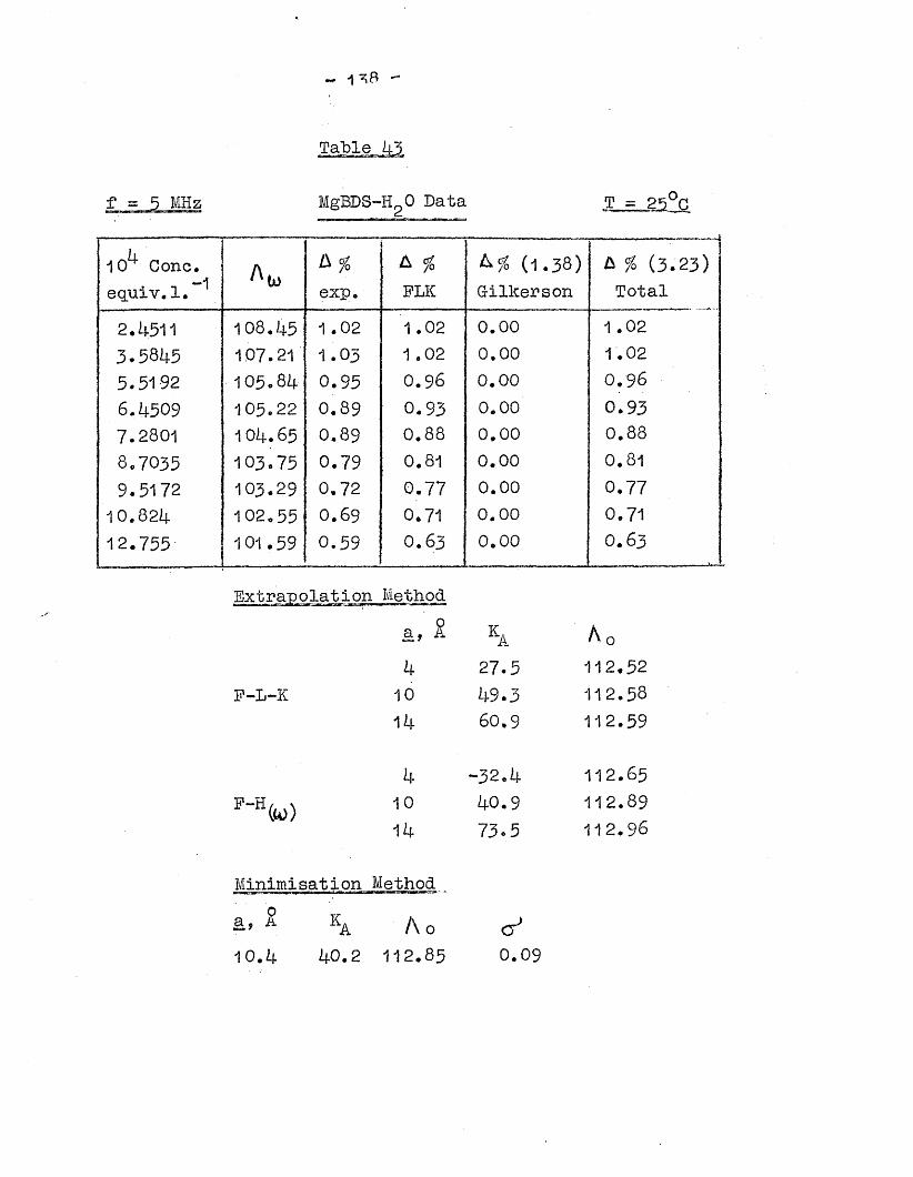
- 1 ^ 8 -

MgBDS-HgO Data T = 2

10 Gone.• n -1equiv.1.

3< A %exp.

A %FLIC

(1 .3 8)G-ilkerson

A % (3.23) Total

2.1+511 108.1+5 1 .0 2 1 .02 0 .0 0 1 .0 2

3.581+5 107.21 1.03 1 .02 0.00 1.025.5192 105.81+ 0.95 0.96 0.00 0.966.1+509 105 .22 0.89 0.93 0.00 0.937.2801 101+. 65 0.89 0.88 0.00 0.888.7035 103.75 0.79 0.81 0.00 0.81

9.5172 103.29 0.72 0.77 0.00 0.7710.821+ 102.55 0.69 0.71 0.00 0.7112.755 101.59 0.59 0 .6 3 0.00 0 .6 3

Extrapolation Methoda, £ ka A 04 2 7 .5 11 2 .5 2

F-L-K 10 1+9.3 112 .58

14 60.9 1 1 2 .5 9

4 -32.1+ 11 2 .6 5

p“H (w) 10 1+0.9 112.8914 73.5 112.96

Minimisation Methoda, £ Ka A 01 0 .4 40.2 112 .85 0.09

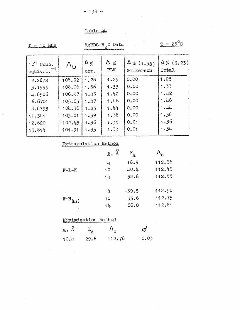
- 139 -

1(A Cone.• i -1equiv.1.

a # :exp.

A, %ELK

(1.38)Gilkerson

(3 .2 3)Total

2.2672 108.92 1 .28 1.25 0.00 1.253-1995 108.06 1.36 1.33 0.00 1.334 .6 5 0 6 106.97 1.43 1.42 0.00 1 .426.6701 105.63 1.47 1 .46 0.00 1.468.8793 104.38 1 .k3 1.44 0.00 1.4411.3U1 103.01 1.39 1 .3 8 0.00 1.381 2 .6 2 0 102.43 1 .3 6 1.35 0.01 1 .3 6

13.814 101.91 1.33 1.33 0.01 1.34

Extrapolation. Methoda, £ ka Ac4 1 8 .9 11 2 .3 6

F-L-K 10 4 0 .4 11 2 .4 3

14 5 2 .6 112.55

4 -39.5 1 1 2 .5 0

F-H(u» 10 33.6 112.7514 66.0 112.81

Minimisation Methoda? £ ka A 0 o ’10.4 29.6 1 1 2 .7 8 0 .0 3

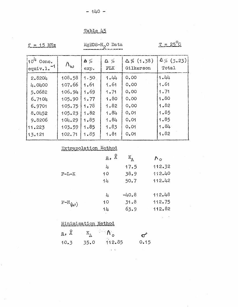
- 140 -

Table 45

MHz MgHDS-HgO Data T = 25°C

10^ Cone.• -T -1equiv.1. Ato

/bexp.

i

(1 %FLIC

(1 .3 8)Gilkerson

(3 .2 3)Total

2.8204 108. 58 1 *5 0... 1.44 0,00 1 .4 44.0400 107.66 1.61 1.61 0.00 1 . 61

5.0682 106.94 1 .6 9 1.71 0.00 1.71

6.7104 103.90 1.77 1.80 0.00 1 .806.9701 105.75 1.78 1.82 0.00 1.828.0452 105.23 1.82 1.84 0.01 1.859.8206 104.29 1,85 1.84 0.01 1 .8 5

11 .223 103.59 1 .8 5 1 .8 3 0.01 1.8413.121 102.71 1 .85 1.81 0.01 1.82

Ao112.32112.40112.42

112.48112.75112.82

a, £ Ka4 17.5

]?-L-IC 10 38.914 50.7

B'-Ha ,) 10 31.84 -40.80 31.814 6 3 .9

Minimisation Methoda, £ xA • A-010.3 35.0 112,85 0.15

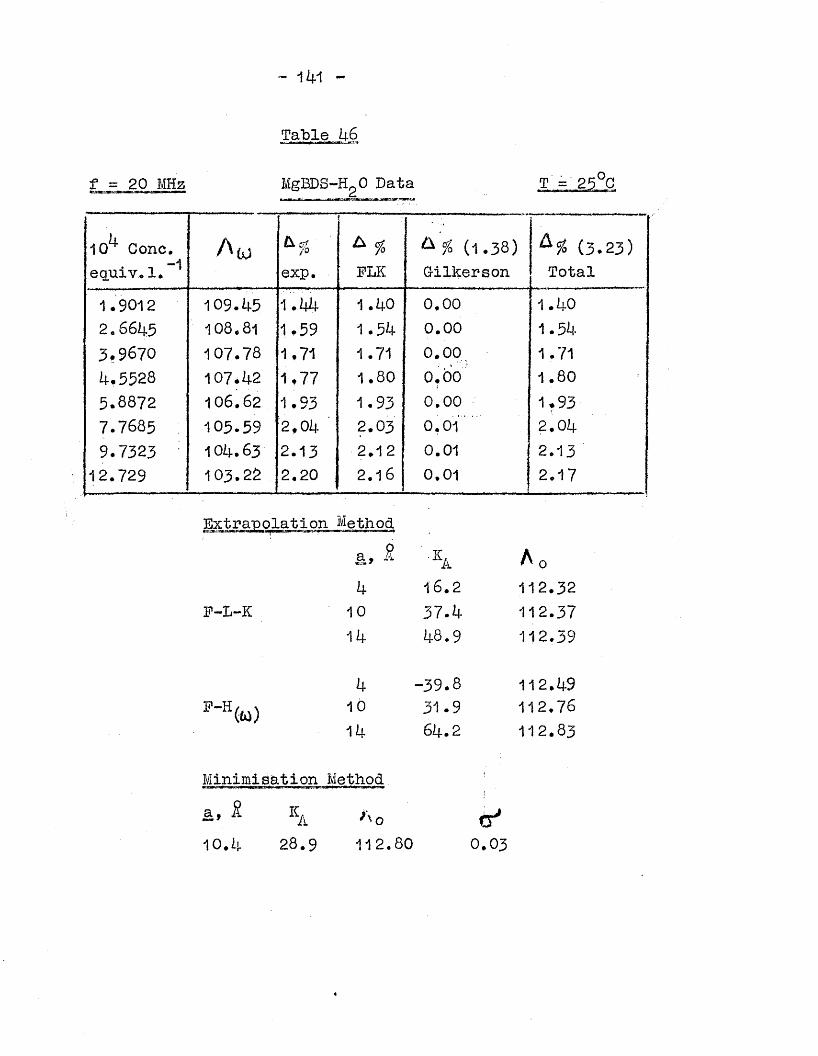
~ 141 -

Tafole 46

f = 20 MHz MgBDS-HgO Data

10 Cone.-•Iequiv. 1.Aui /o

exp.

f^ %FLK

(1.38)G-ilkerson

(3 .2 3)Total

1.9012 109.45 1 *44 1 .40 0,00 1.402.6645 108.81 1,59 1.54 0.00 1.543.9670 107.78 1*71 1.71 0.00 1.714.5528 107.42 1*77 1.80 0.00 1.805.8872 106.62 1.93 1.93 0.00 1.937.7685 : 105.59 2,04 2.03 0.01 2.049.7323 104.63 2.13 2.12 0.01 2.13

12.729 103 .2 2 2.20 2 .1 6 0.01 I2.17

Extrapolation Methoda, 8. ka Ao4 1 6 .2 1 1 2 .3 2

F-L-K 10 37.4 1 1 2 .3 7

14 48.9 112 .39

4 -39.8 112 .49

F-H(U ) 10 31.9 112.7614 64.2 112.83

Minimisation Method

^ KA a o cr*10. 4 28.9 112.80 0 .0 3

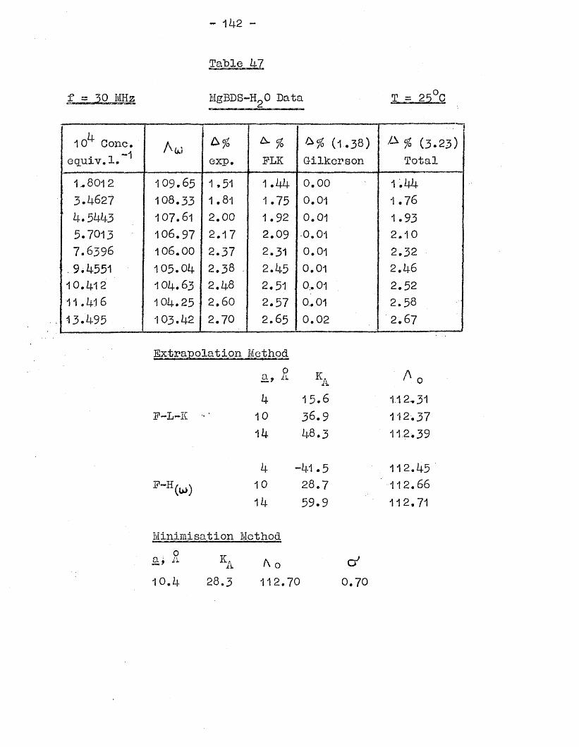
10 Cone.• i -1equiv.1.

Aw Mexp.

A- % FLK

(1.38)Gilkerson

a % (3 .2 3)Total

1.8012 1 0 9 .6 5 1.51 1.44 0.00 1.443.4627 108.33 1.81 1.75 0.01 1.764.5443 107.61 2.00 1.92 0.01 1.935.7013 106.97 2.17 2.09 ■0.01 2.107.6396 106.00 2.37 2.31 0.01 2.329.4551 105.04 2.38 . 2.45 0.01 2.46

10 .41 2 104.63 2.48 2.51 0;. 01 2.5211.416 104.25 2.60 2.57 0.01 2.5813.495 103.42 2.70 2.65 0.02 2.67

Method

F-L-K

ak1011*

0ka

15.636.948.3

/Vo 1.12.31 1 1 2 .3 7112.39

F-H(W)1*

10

11*

-1*1.528.759.9

112.1*5112.66112.71

Minimisation Method 0a

10.4KA

28.3A o 112.70

&0.70

- 1A3 -

Table A8

f = kO MHz HgEDS-HgO Data _T_2,

. ■ ••••...- I10 cone.

• -1 eguiv.l. | N exp./\ 07" /OFLK

i ■ — ~~ “! h ?o (1 .3 8)Gilkerson

u----------£70 (3 .2 3)Total

3.9256 I 108.17 2.03 1.94 0.01 1.95A.5i+A5 I 107.79 2.12 2.05 . 0.01 2.065.A691 | 107.21 2.20 2.20 0.01 2.215.9978 | 106.92 2 . 27 2.27 0.01 2 .2 8

7.8672 j 106.03 2.54 2.52 0.01 2.5311.213 i 10A.53 2.77 2.77 0.02 2.7913.061 ! 103.82 2.89 2.90 0.02 2.9214.202 j

!1 0 3 .3 6 2.95 2.95 0.02 2.97

Tl'ictra'polatioii Methoda, 2 K^ A0k 17.2 112.33

F-L-K 10 39.2 112.A21k 5 0 .6 112.A5

P-Hkill ^ -38.7 112.5110 3A.7 112 .8 21A 6 6 .6 112.89

Minimisation Methoda., £ A 010.5 26.1 112.82 0.51

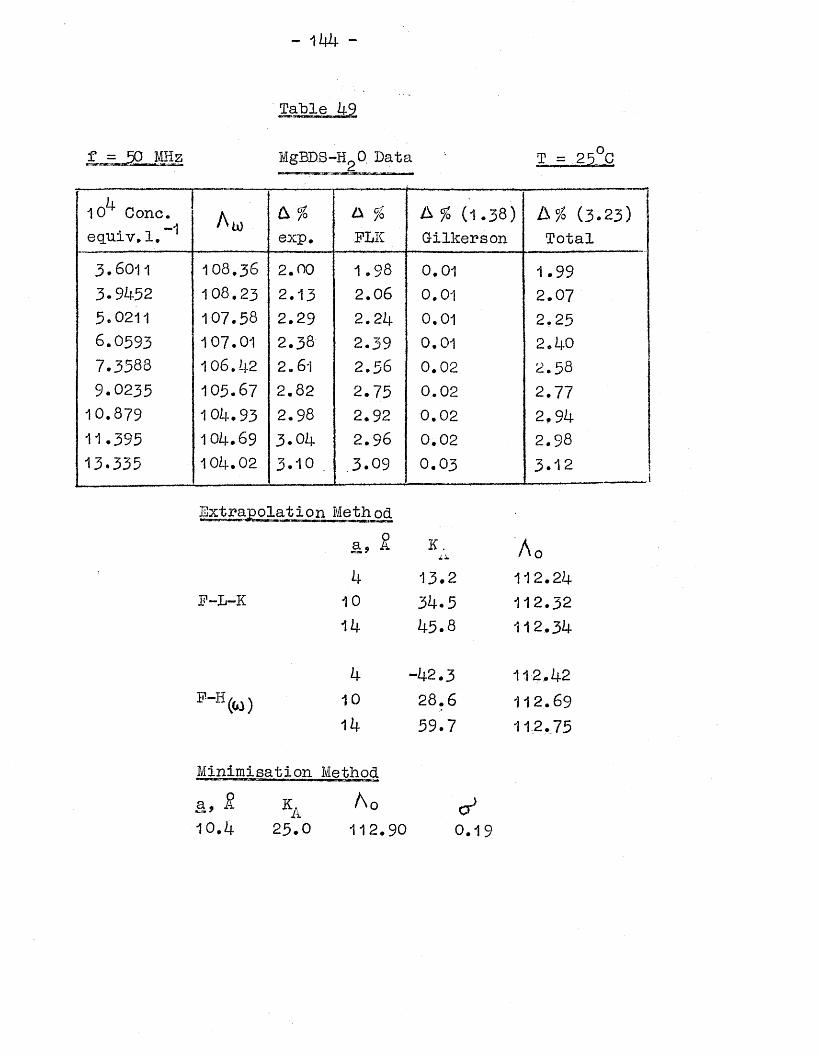
- 144

Table 49

f = 50 MHz MgBDB-HgO. Data

10 Cone, equiv, X. Aw I\ %

exp.A %FLIC

A # (1.38) Gilkerson

A # (3.23) Total

3.6011 108.36 2.00 1 .98 0.01 1.993-9452 108.23 2.13 2.06 0.01 2.075.0211 107.58 2.29 2.24 0.01 2.256.0593 107.01 2.3& 2.39 0.01 2.407.3583 106.42 2.61 2.56 0.02 2.589.0235 105.67 2.82 2.75 0.02 2.7710.879 104.93 2.98 2.92 0.02 2,9411.395 104.69 3.04 2.96 0.02 2.9813.335 104.02 3.10 . .3.09 0 .0 3 3.12

...

Extrapolation Methoda, R K,X * A o4 13.2 112.24

F-L-K 10 34.5 1 1 2 .3 2

14 45.8 112.34

4 -42.3 112.4210 28.6 112, 6914 59.7 11,2.,. 75

Minimisation\

MethodAo V

10.4 25.0 112.90 0.19

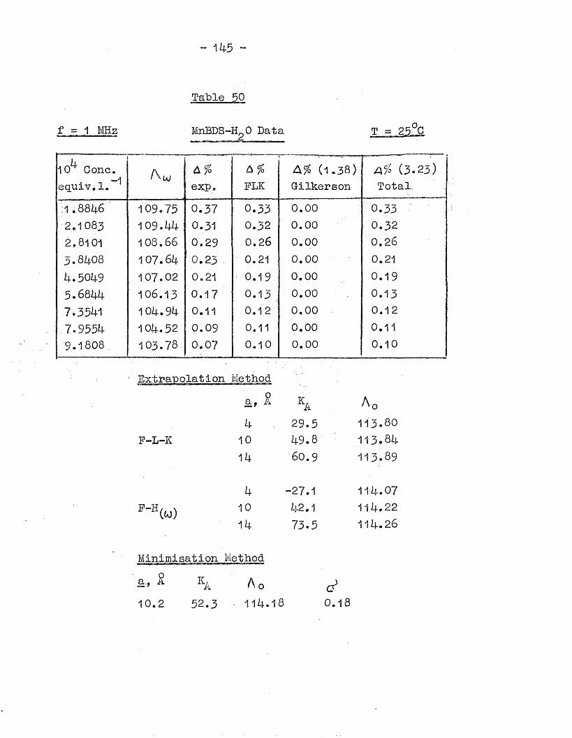
- 145 -

f = 1 MHz MnBDS-HgO Data

10 Cone.-1equiv.1. exp.

6 % FLK

(1.38)Gilkerson

A% (3.23)Total..

:1; 8846 109.75 0.37 0.33 0.00 0.332.1083 109.44 0.31 0.32 0.00 0.322.8101 108.66 0.29 0 .2 6 0.00 0 .2 6

3.8408 107.64 0.23 0.21 0.00 0.214.5049 107.02 0.21 0.19 0.00 0.193.6844 106.13 0.17 0.13 0.00 0.137.3541 104.94 0.11 0.12 0.00 . 0.12.7.9554 104.52 0.09 0.11 0.00 0.119.1808 103.78. 0.07 0.10 0.00 0.10

Method

F-L-K

F-H(«)

& ka Ao4 29.5 113.8010 49.8 113.8414 60.9 113.89

4 -27.1 114.0710 42.1 114.2214 73.5 114.26

Minimisation Method £ Ka, a

10.2A A o

52.3 114.18 0.18

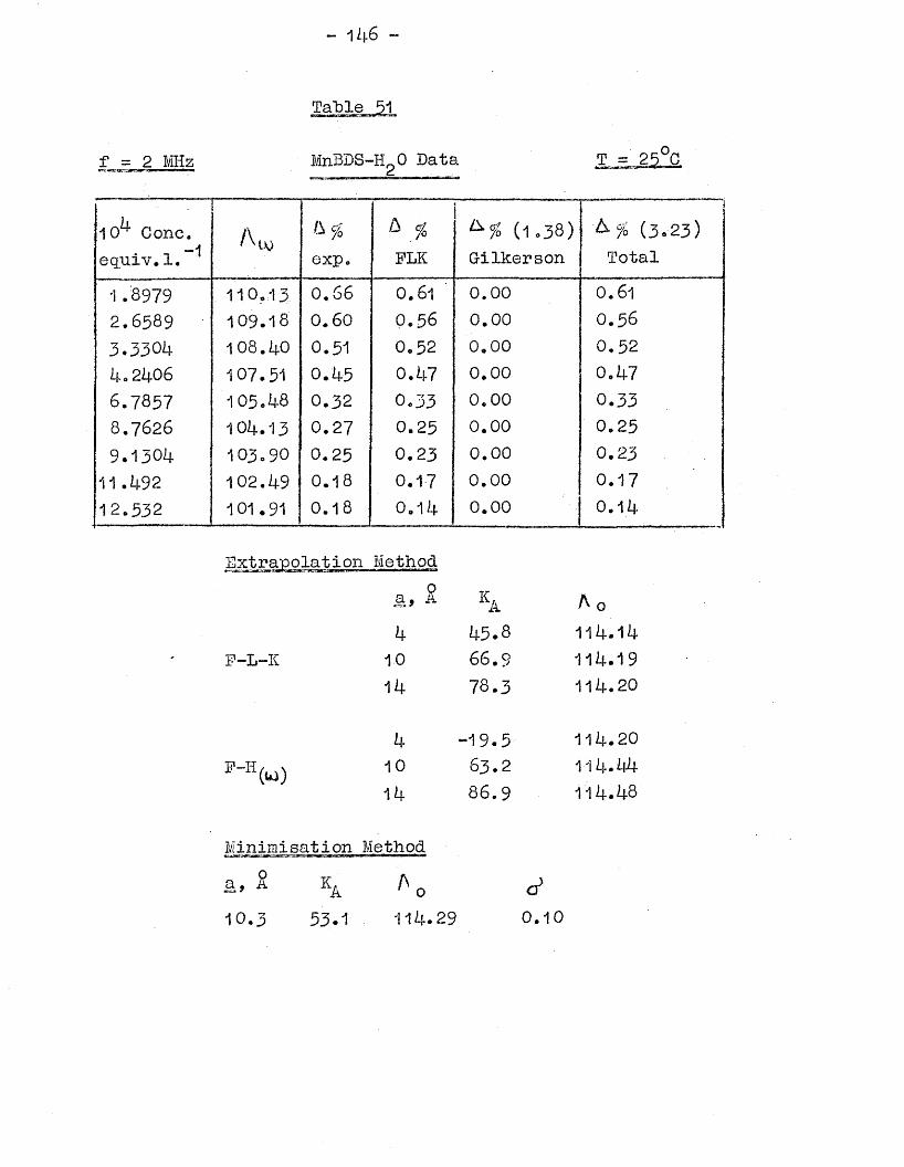
f = 2 MHz MnBDS-HgO Data T =

10^ Cone, equiv.1. Au> M

exp.A %FLK

& % (1.38) Gilkerson

(3.23) Total

1.8979 110.13 0.66 0.61 0.00 0.61

2.6589 109.18 0.60 0.56 0.00 0.563.3304 1 0 8 .4 0 0.51 0.52 0.00 0.524.2406 107.51 0.45 0.47 0.00 0.476.7857 105.48 O.32 0.33 0.00 0.338 .7626 104.13 0.27 0.25 0.00 0.259.1304 103 .90 0.25 0.23 0.00 0.2311.492 102.49 0.18 0.17 0.00 0.1712.532 101.91 0.18 0.14 0.00 0.1 4

F-L-K

F-II(W)

0a, a K.ir3u A 04 4 5 .8 114.14

10 6 6 .9 114.1914 78.3 114.20

4 -19.5 114.2010 6 3 .2 114.4414 86.9 114.48

Minimisation MethodAa

10.3ka53.1

o114.29

o’0.10

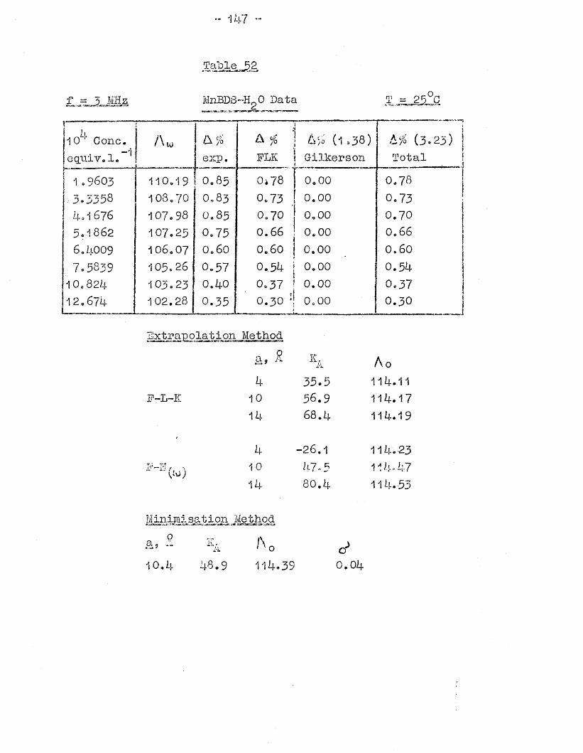
- 147 -

TaSl§J52

f =. 5. M & MnBDS-HgO Bata S.J0^£S.

V — ....]_}

10 ‘ Cone. A w /A %i

A $ ! A>o (1.38) (3 .2 3) |-j -1equiv. 1. I exp. FLK ! Gilkerson1 Total !.. .

1 .9603 110.19 O.8 5 0J8 j 0 .0 0 0.78 j3.3358 108.70 0 ,8 3 0.73 1 0 . 0 0 0.7 34.1 676 107.98 ! 0o85 0 .7 0 j 0 ,0 0 0.705,-1862 107.25 0.75 0.66 ! 0 .0 01 0.666.4009 106.07 O060 0.60 j 0.00 0.607.5839 105.26 0.57 0.54 ! 0.00 I 0.5410.824 103.23 0.40 0.37 f 0.00 0.371 2.674 102.28 0.35 0.30 0 .0 0 0 .3 0

Extrapolation Methoda, A K,.O A 04 35.5 114.11

F-L-K 10 56.9 114.1714 68.4 114.19

4 -26.1 114.23E-Hz', '

\ I m )10 47-5 114 .4 7

Minimi sat i on

14

Method

8O. 4 114.53

a , S K,•TA. Ao

10.4 48.9 114.39 0 .0 4

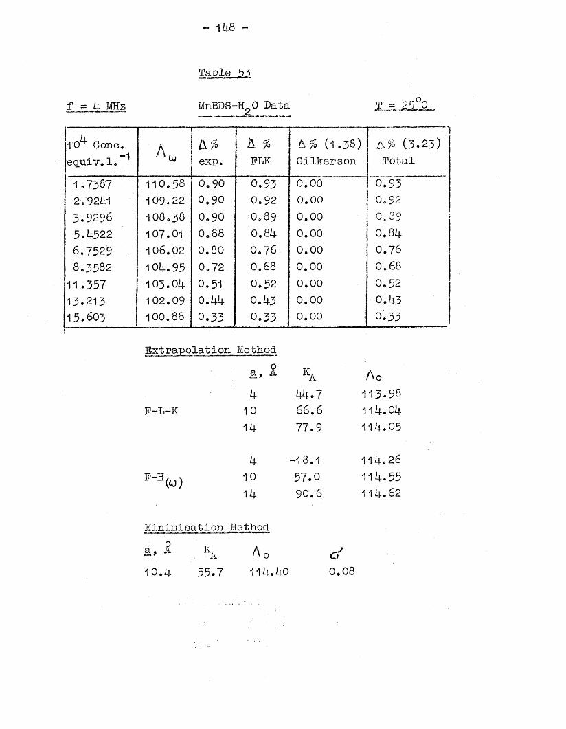
- 148 -

Table 55

MnEDS-HgO Data o.T1=_25 C

10 Cone._-teguiv.l.IX %

exp.A %FLK

/3 (1 .3 8)G-ilEerson

M ’° (3.23)Total

1.7387 110.58 0.90 0.93 0.00 0.932.9241 109.22 0.90 0.92 0.00 0.923.9296 108.38 0.90 0.89 0.00 0.395.4-522 107.01 0.88 0.84 0.00 0.846.7529 106.02 0.80 0.76 0.00 0.7 68.3582 104.95 0.72 0.68 0.00 0.6811.357 1 0 3 .0 4 0.51 0.52 0.00 0.5213.213 102.09 0.44 0.43 0.00 0.4315.603 100.88 0.33 0.33 0.00 0.33

Extrapolation Method

F-L-K

F-H(«)

a, £ ka Ao4 44.7 113.9810 66.6 114.0414 77.9 114.05

4 -18.1 114.2610 57.0 114-5514 90.6 114.62

Minimisation Method

&> 5 ka A o o '1 0 . 5 5 . 7 111).. 40 0.08

- 149 ~

.

10 Cone.• i -1equiv.1. A * exp.

A jS FLK

A ^ (1 .3 8 )Gilkerson

A # (3 . 2 3 )Total

1.9283 110 .3 9 1..04 1.01 0.00 1.013.2288 108 .9 6 0 .9 8 1.01 0.00 1 .015 .2168 1 0 7 .2 3 0.90 0.96 0.00 0 .9 6

6.7634 106.16 0.92 0.88 0.00 0.88

7.6517 105.48 0.79 0.85 0.00 0,858.9401 104.60 0.77 0.78 0.00 0.78

10.401 103.76 O.6 9 0.71 0.00 0.7112.145 102.69 0.62 O.63 0.00 O.6 3

,14.063 10 1 .74 0.52 0.55 0,00 0.5516/040.. . . ......

100.76 0.42 0.47 0.00 0.47

F-L-K

F-H

a, S. ICA A 04 4 2 .9 114.27

10 64.2 114.3414 80.0 114.35

4 -15.2 114.3210 62.6 1 1 4 .6 4

14 96.5 114.72

Minimisation Methoda, R K,10. 4

A 46.1

Ao1 1 4 .3 9

aJ 0 .1 4

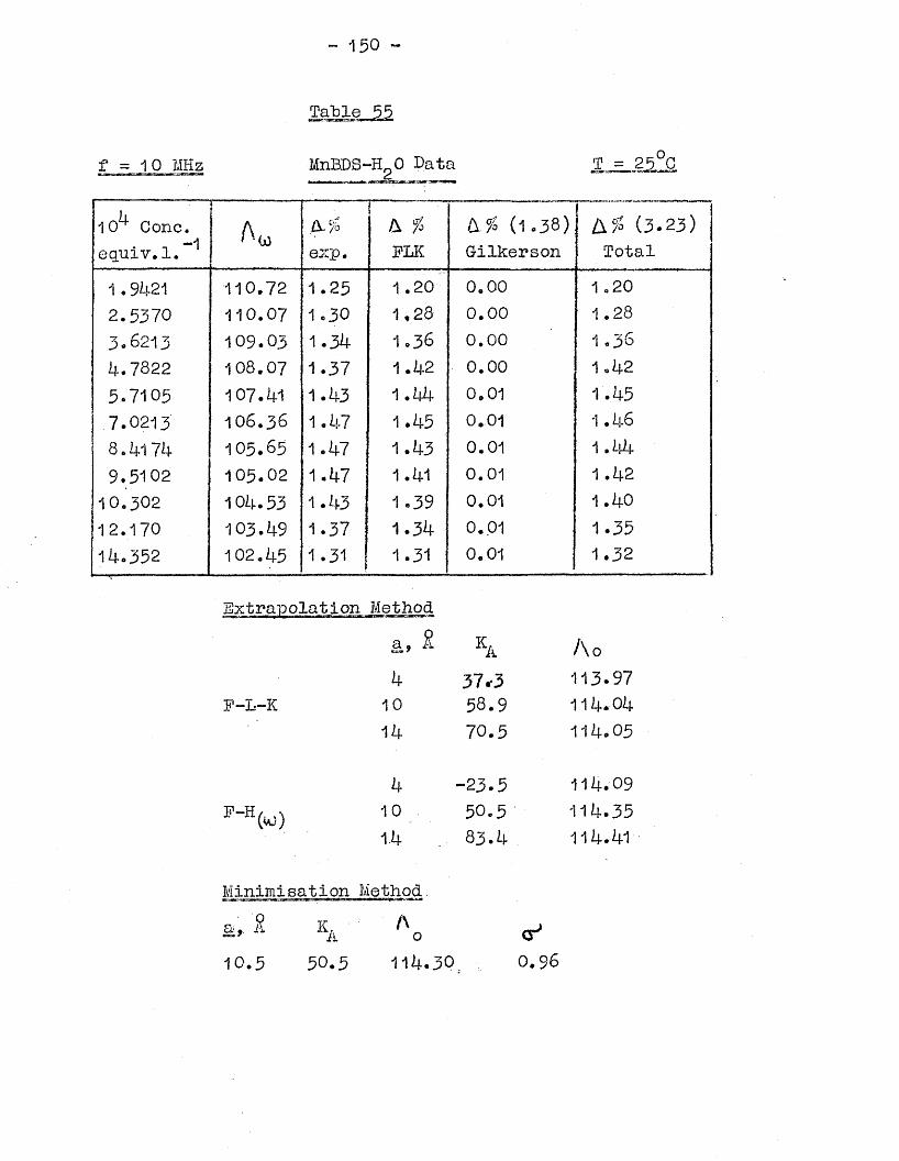
- 150 ~

Table 55

f = -I0 MHz MnEDS-H 0 Data T = 25°C

10^ Cone.-1equiv. 1.

3C A-%exp.

rA %FLK

(x% (1 .3 8)Gilkerson

L % (3.23)Total

1 ♦9421 110 .7 2 1.25 1 .20 0.00 1 .202.5370 1 1 0 .0 7 1.30 1,28 0.00 1.283^6213 1 0 9 .0 3 1-34 1.36 0.00 1 .364.7822 108.07 1.37 1 .42 0.00 1.425.7105 107.41 1.43 1.44 0.01 1.457.0213 106.36 1.47 1.45 0.01 1 • 468.4174 105.65 1.47 1.43 0.01 1.449.5102 1 0 5 .0 2 1.47 1.41 0.01 1.42

10 .302 104.53 1.43 1.39 0.01 1.4012.170 103 .49 1.37 1.34 0.01 1.3514.352 102.45 1.31 1.31 0.01 1.32

a, R ka Ao4 37 *3 113 .97

■F-L-K 10 58.9 1 1 4 .0 4

14 70.5 114.05

4 -23.5 114.09p-H(«) 10 50.5 114.35

1.4 83.4 114-41

Minimisation Method.a, R V A

0 cr*10.5 5 0 .5 11 4 .3 0 0 .9 6

- 151 -

f = 1 5 MHz MnEDS-HgO Data JjL=

10 Cone, equiv. 1.

!A,i

ti%exp.

j 6 %FLIC

11 % (1.38) Gilkerson

- ---------------

H% (3.23) Total

1.8254 110 .9 6 1.33 1 .30 0.01 1 .313.1477 1 0 9.66 1.52 1 .52 0.01 1.334.7901 108.40 1.71 1.67 0.01 1.686.3926 107.29 1.78 1 .76 0.01 1.777.3105 10 6 .6 7 1.77 1.79 0.02 1.81

8.7559 105.82 1 .8 3 1.82 0.02 1.8410.002 105.12 1 .8 3 1 .8 3 0.02 1.8511.495 104.29 1 .8 3 1 .82 0.02 1.8412.275 103.91 1.82 1 .81 0.02 1 .8 313.676 103.27 1.81 !1.80 0.02 1.82

Extrapolation Methoda, 2. ka > 0

.

4 37.9 114 .0 2

F-L-K 10 59.4 114 .09

14 70.9 1 1 4 .1 0

4 -22.3 1 1 4 .1 6

F"H(C0) 10 50.9 114.3914 63.5 114.48

Minimisation MethodP rr a y J&. 4 cr'

10.4 45.0 114.30 0 .2 4

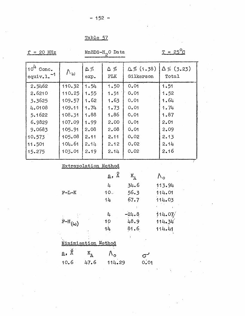
- 152 -

Table 57

f = 20 MHz MnBDS-HgO Bata

10 Cone.—1equiv.1. A to l\%

exp.a fo FLK

Afo (1.38) Gi Ike a? son

& % (3 .2 3)Total

2.51+62 110.32 1.54 1 .50 0.01 1*512.6210 110.25 1.55 1.51 ' 0.01 1*523.3625 109.57 1 .6 2 1.63 0.01 1.61+4.01 08 109.11 1.74 1.73 0.01 1.745.1622 108.31 COCO• 1.86 0.01 1.876.9829 107.09 1-99 2.00 0.01 2.019.0683 105.91 2.08 2.08 0.01 2.0910.573 105.08 2.11 2.11 0.02 2.1311.501 104.61 2.14 2.12 0.02 2.1415.275 103.01 2.19 2.14 0.02 2 .1 6

F-L-K

(<*»}

Methoda, ka Ao4 31+.6 113.9410-. 56.3 114.0114 67.7 114.03

4 -24.8 114.07;10 48.9 114.3414 81.6 114.41

Minimisation MethodS. ? S. 10*6

ka47.6

Ao111+. 29

c r 1o.oi

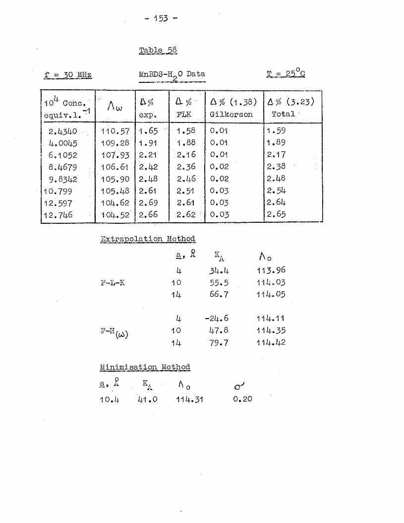
- 153 -

f = 50 MHz. MnBDS-H^O Data T = 25°G

10^ Coho.• i -1equiv.1. ;

3< IX %exp.

a . %FLK

A % (1.38)G-ilkerson

h % (3 .2 3)Total

2,4340 110.57 1.65 1.58 0.01 1 .594.0045 109.28 1.91 COCO« 0.01 1 .896.1052 107.93 2.21 2 .1 6 0.01 2.17S.i+679 106.61 2.42 2 .3 6 0.02 2.389.8342 1 0 5 .9 0 2.48 2 .4 6 0.02 2.48

10.799 105.48 2.61 2.51 0.03 2.5412.597 104.62 2.69 2.61 0.03 2.6412.746 104.52' 2.66 2.6 2 ' 0 .0 3 2.65

Extrapolation Methoda, A ka A 04 34.4 1 1 3 .9 6

F-L-K 10 55.5 114.0314 66.7 1 1 4 .0 3

4 -2 4 .6 114.1110 47.8 114.3514 79.7 1 1 4 .4 2

Minimisation Methoda <i S. ka cK1 0.4 41 .0 114.31 0 .2 0

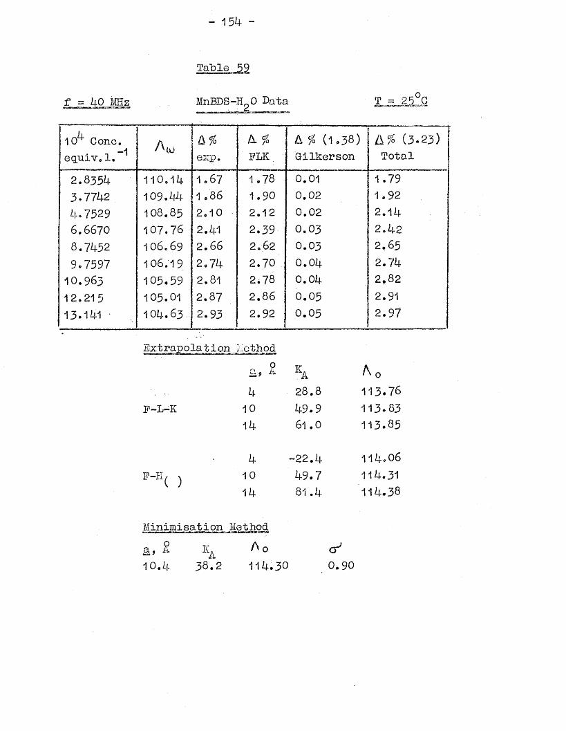
- 134 -

f = 40 MHz MnBDS-PI-0 Data T = 25°C

10 Cone.•t -1equiv. 1, Au_i

------& %0XjP e

A. % FLK.

A % (1.38) Gilkerson

....... “ ~"i(3 .2 3)

Total2.8354 1 1 0 .1 4 1.67 1.78 0.01 1.793-7742 1 0 9 .4 4 10 86 1.90 0.02 1.924.7529 108.85 2.10 2.12 0.02 2.146.6670 107.76 2.41 2.39 0.03 2.428.7452 10 6 .6 9 2.66 2 .6 2 0.03 2,659.7597 106.19 2.74 2.70 0.04 2.74

10 .963 105.59 2.81 2.78 0.04 2.8212.215 105.01 2.87 2.86 0.03 2.9113.1U1 1 0 4 .6 3 2.93 2.92 0.03 2.97

Extrapolation Method90. y 2-i. ka Ao

4 28.8 1 1 3 .7 6

10 49.9 1 1 3 .8 3

14 6 1 .0 11 3 .8 5

4 -22.4 1 1 4 .0 6

10 49.7 114.31

14 8 1.4 114 .38

Minimisation Methoda, 2 K. Ao oJ10.4 38.2 114.30 0.90

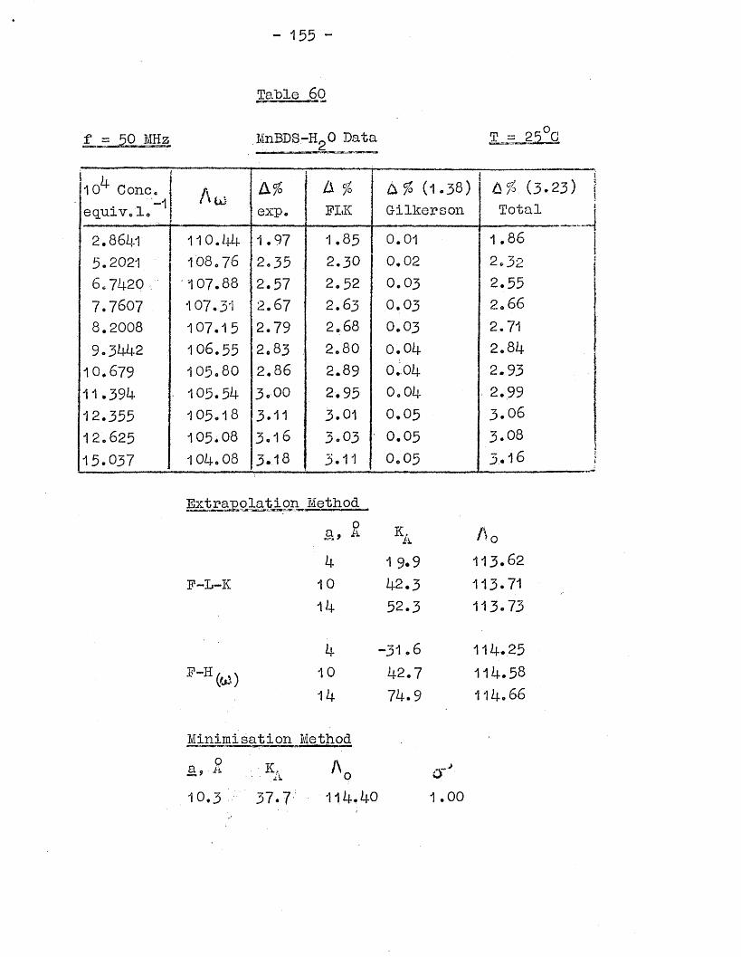
- 155 -

Table 60

MnEDS-HgO Data

[ I,lO4' Gone.,• -1 "1equiv.1. Aui exp.

l\ fo KLK

(1.38)G-ilkerson Tot

2.8641 11o.44 1.97 1.85 0.01 1 .8 6

5.2021 108 .76 2.35 2.30 0 .0 2 2.326 .7 4 2 0 . '107 .88 2.57 2 .5 2 0 .0 3 2.557.7607 107.31 2.67 2 .6 3 0 ,0 3 2.668.2008 107.15 2.79 2.68 0 .0 3 2.719.3442 106.55 2.83 . 2.80 0.04 2 08k10.679 105.80 2.86 2.89 0.0k 2.9311.394 ■ 105.54 3.00 2.95 0 ,0 4 2.9912.355 105.18 3.11 3.01 0.05 3.0612.625 105.08 3 .1 6 3.03 0.05 3.0815.037 104.08 3. .18 3.11 0 .0 5 3 .1 8

Extrapolation Methoda, iS: ka Ao4 1 9 .9 11 3 .6 2

F-L-K 10 4 2 .3 113.7114 5 2 .3 113.73

k -3 1 .6 11 4 .2 5

F“H («) 1014

42.774.9

114 .5 8 114.66

Minimisation Methoda j ii K,.ii. \ o-J10.3 37.7 1 1 4 .4 0 1 .0 0

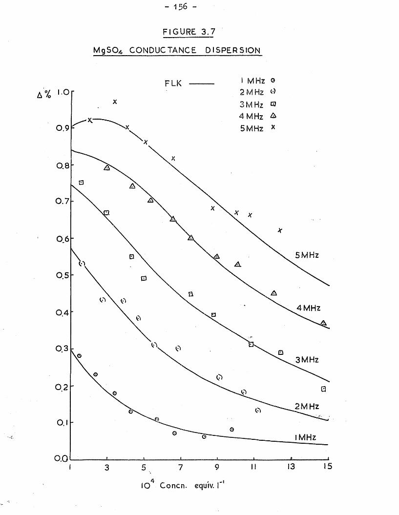
- 156 -

FIGURE. 3 .7

MgSCU CONDUCTANCE DISPERSION

FLK --------- 1 MHz ®2 M HzA %

4 MHz ^5 MHz *0.9

0 .7

0.65MHz

0.5

4 MHz0.4

0 33 MHz

0 22MHz

I MHz

0.01513973 5

4 < -iIO Concn. equiv. 1

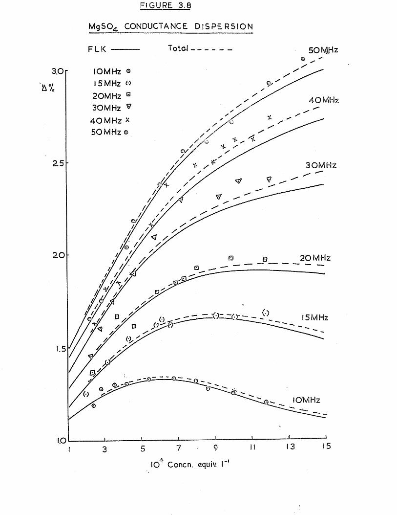
FIGURE 3.8

MgSO^ CONDUCTANCE DISPERSION

3.0 r

7•o

2.5

2.0

FLK --------

lOMHz © 5 MHz w

20MHz B 3 0 MHz *

4 0 M H z * 50M Hz

Total-------- 50K4Hz

20 MHz

X9z_ y.)i- - J

a.lO'MHz

1.03 7 II 3 5

lO4 Goncn.

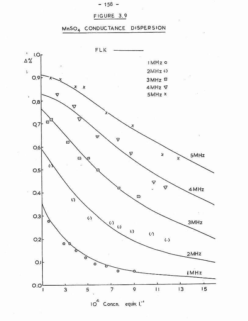
- 158 - FIGURE 3,9

M n S Q 4 CONDUCTANCE DISPERSION

FLK-Or

2MHz O

5MHz

Q7

0.65MHz

0.5

4 MHz0.4

0.33MHz

0.2

2 MHz

M H z

0.0

4-O Concn. equiv. 1.'

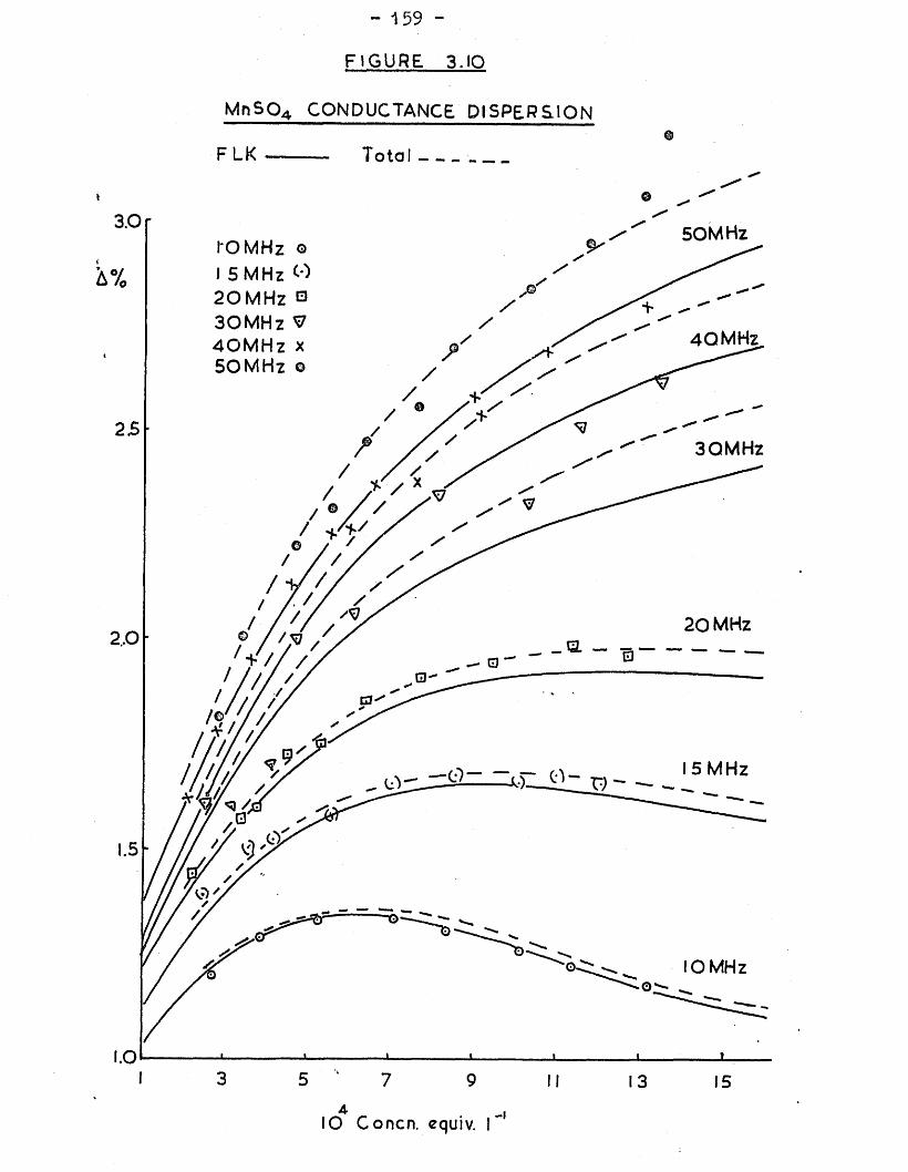
- 159 -

FIGURE 3 . IQ

MnSQ4 CONDUCTANCE DISPERSION

FLK T o ta l ------

50 MHz1*0 MHz o I 5 MHz O 2 0 MHz ° 30 M H z V 4 0 M H z x 50 M H z ©

40M H z

30M H z

20 MHz

5 MHz

lOMHz

10 Concn. equiv. -i

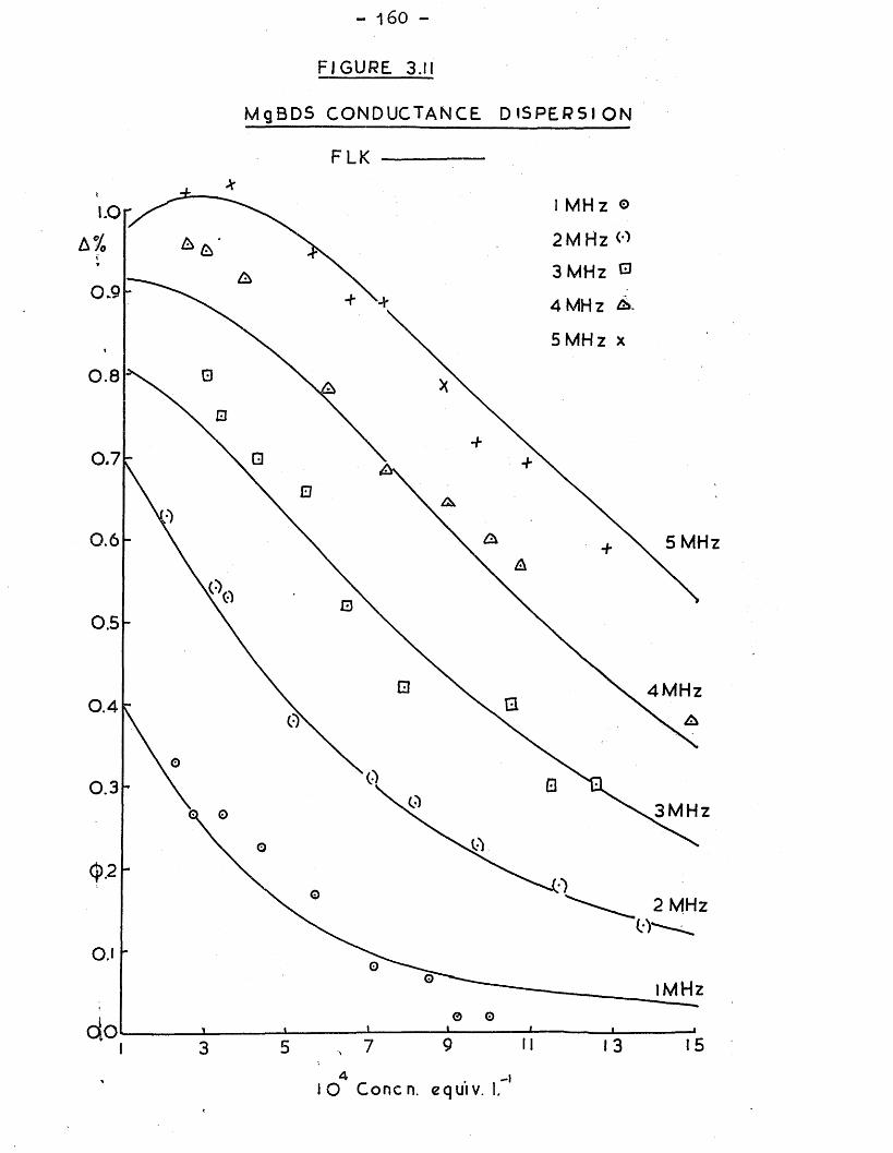
- 16o -

FIGURE 3.II

MgBDS CONDUCTANCE D IS P E R S IO N

FLK

I MHz ©

2 MHz O

3 MHz GJ

4 MHz

LO

5 MHz x

0.8

0.7

0.6 5 MHz

0.5

4M H z0.4

0.33M H z

2 MHz

O.ilMHz

4I O Cone n. equ'iv. I.

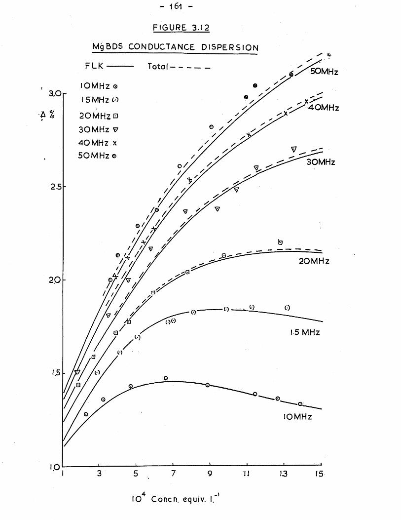
- 1 6 - 1 -

FIGURE 3.12

MgBDS CONDUCTANCE DISPERSION

Total---------------50MHz

OMHz o

I 5 MHz O

2 0 M H z 0 30M Hz

4 0 MHz SOMHz

^ 4 . 0 M H z

30MHz

20M H z

oIOMHz

, _4 , -l10 Concn. equiv. I.

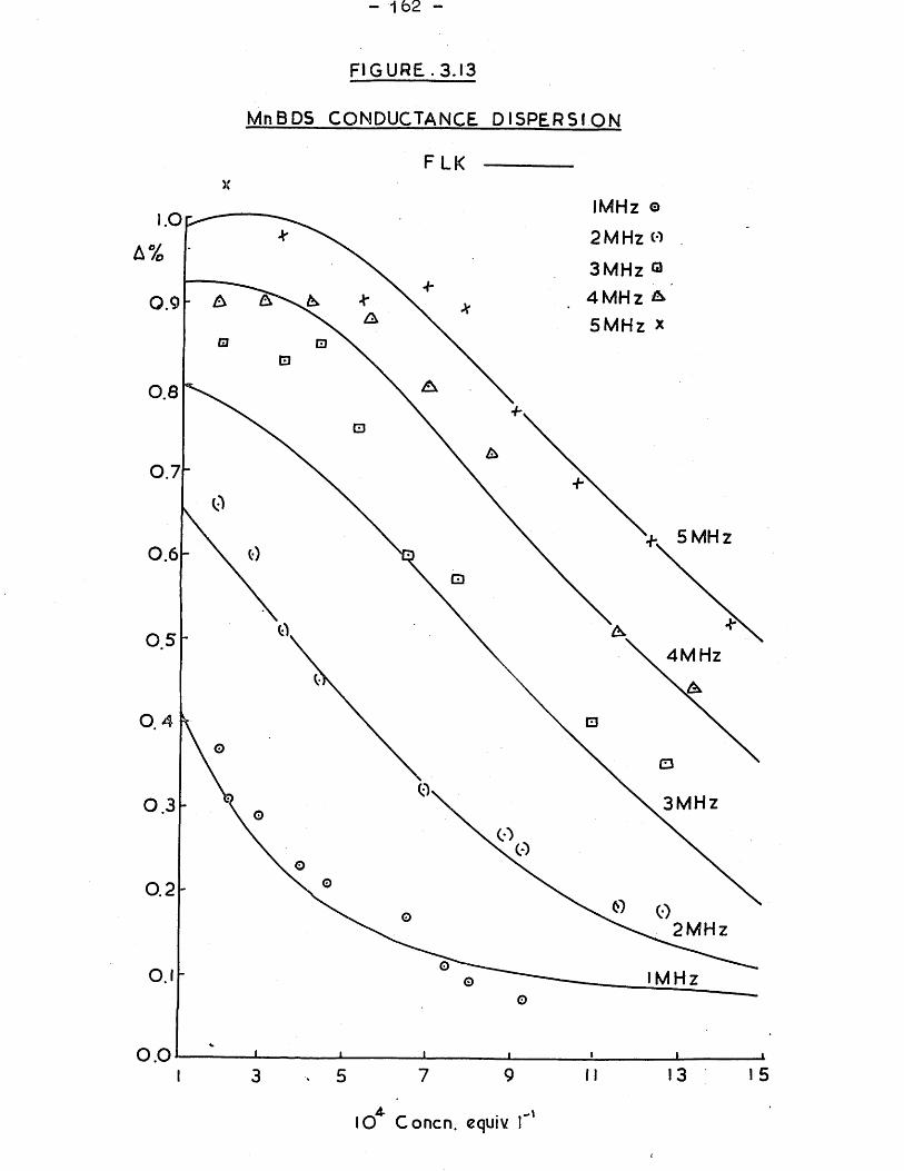
- 1 62 -

FIGURE. 3.13

MnBDS CONDUCTANCE DISPERSION

FLKx

IMHz ©

2 MHz to

3MHz Q 4 MHz 5M Hz x

A%

0.9

0.8

0.7

5 MHz0.6

0 54MHz

0 .4

3MHz0 .3

0.22MHz

O.l IM Hz

0.0I 5I 3975 II3

IO * Concn. equiv f*

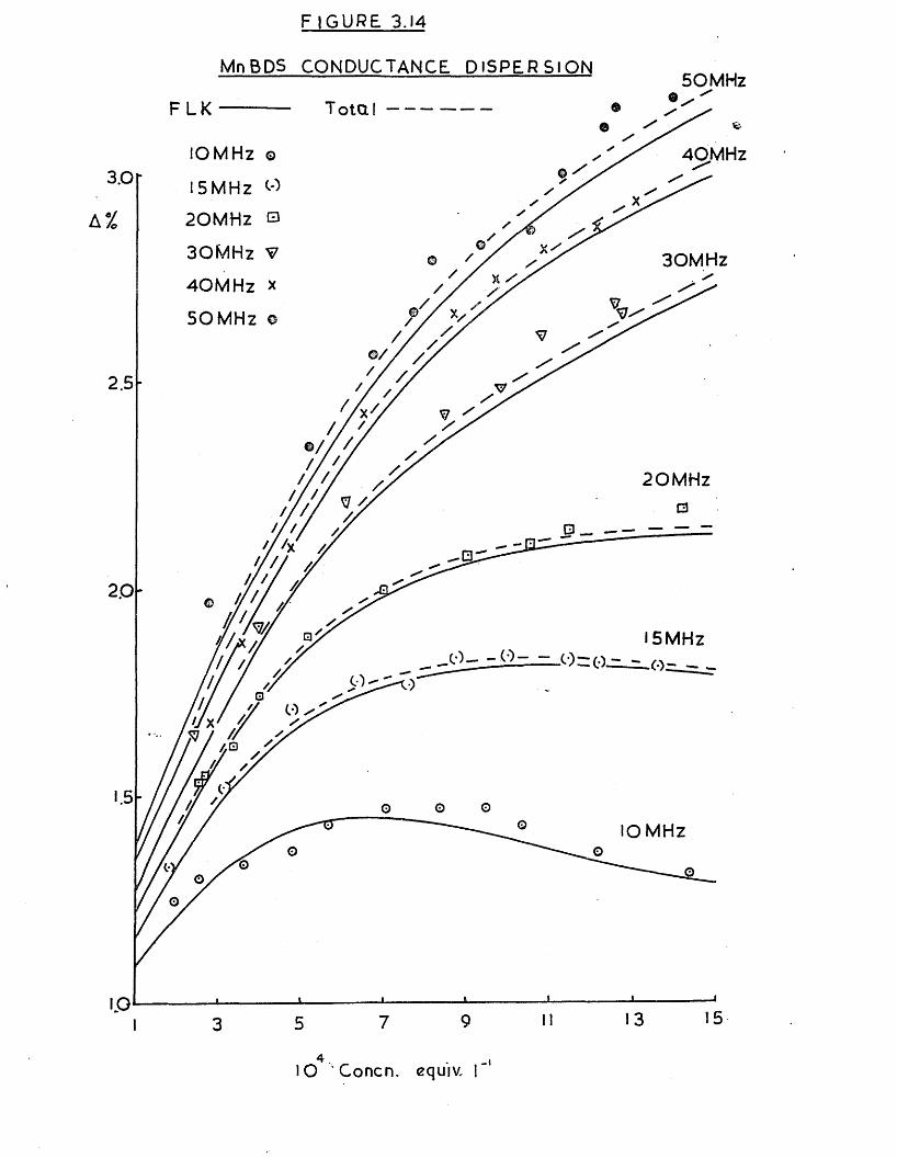
F 1GURE 3.14MnBDS CONDUCTANCE DISPERSION ---------------------------------------------------------------- 50MHz

lOMHz ©

15MHz CO

20M Hz 0

30M Hz V

40MHz

30MHz40M H z *

20M H z

15MHz

IO Concn. equiv, I

PART III SECTION 3

DISCUSSION OF RESULTS

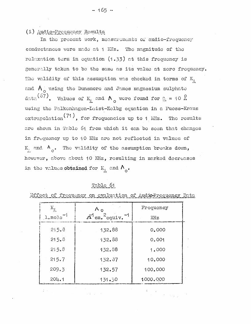
- 165 ~

(i) Audio-Prc quency _ Re suit sIn tlio present work, measurements or audio-fre quency

conductances were made at 1 KHz, The magnitude of therelaxation term in equation (1«33) at this frequency isgenerally taken to he the same as its value at zero frequency.The validity of this assumption was checked in terms ofand A 0 using the Dunsmore and James magnesium sulphateaata^ 7) Values of K, and A were found for a = •] o £A ousing the Palkenliagen-Leist-Kelhg equation in a kuoss-ICraus

(71 )extrapolation , for frequencies up to 1 mHz. The resultsare shown, in Tahle Si from which it can ho seen that changesin frequency up to 10 KHz are not reflected in va.lucs ofK, and A e The validity of the assumption breaks down, x- ohowever, above ahout 10 KHz, resulting in marked decreasesin the values obtained for K, and A *n o

Table J>1Hffect of frequency on evaluation of AudIb-ffrc quency Data

A cm. equiv

132.88132.88132.88

0.000215 0.001215 1 .00 0

10 .000

100.0001000,000

— 166 -

The results for magnesium and manganese (II) sulphatesand benzenedisulphonates measured in this work are shownin Tables 12 to 16. ‘Table 12 lists IC, and A valuesn ocorresponding to a-values of Ij., 10 and 1k £ using theextrapolation function (3*17). For the four electrolytesstudied the standard deviation of the extrapolation plotsgave variations of the order of 0.08 o in A q and 0,5/° i*1It is interesting to note that for the benzenedisulphonatesalts it is possible to obtain degrees of dissociationgreater than unity and correspondingly negative values,for a parameter values of the order of k -S. This is aconsequence of the decrease in A with decreasing a andsetting ok equal to A /A . /mother feature of Table 12expis that the complete Fuoss-Hsia equation usually yields values of A significantly larger than those given by the Falkcnhagen-Leist-Kelbg and Pitts equations.

The results of minimisations on the audio-frequency data by the complete and modified forms of the Pitts and Fuoss- Hsia equations are shown in Tables 13 to 16. The best-fit values of the three parameters K^, A Q and a are listed for each equation together with the corresponding values of the variance,CT*, defined by :

cr' = (s2A F ......... (3-22)2'where N is the number of data points and S * is the sum of

the squared deviations between experimental *and calculated conductances (equation 3.18).

- 167 -

It was noted that the minimising (\ values for the complete Fuoss-Hsia equation were always greater than those values obtained using the other equations. In the case of the magnesium sulphate data a A q value of 133*37 was obtained which was unacccptably high in comparison with the literature values (see below) and so A was fixed at 133*07 for the complete and modified Fuoss-Hsia equations. This resulted in a relatively poor fit (cr* = 0 ,1 6) with the complete equation. In general? the two forms of the Pitts equation always yielded smaller (\Q and a values than those obtained using the Fuoss-Hsia equations* The differences between the complete and modified forms of each equation in terms of their minimising parameters are very small. Hence the

7 / oeffect of neglecting the incomplete terms above c has a very small effect on KA ? A and a.

It is useful to compare the audio-frequency results for , A und a with the experimental values obtained by other investigators using various measurement and evaluation methods. Each electrolyte will be considered in turn; the IC. values are rounded off to +0.5.

i*x

Magnesium SulphateThe results of the present work on magnesium sulphate

are shown in Table 62 and the results of other workers are listed in Table 63. The values of K, that were obtained by1'Xconductance in Table 63 wore derived from the same

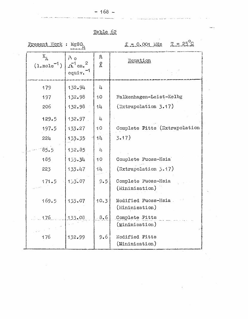
- 168

Tefcle 62«jtT7«-..aa m ,»1 i la.,'

Present Work : MgSO^ f j=l,Q.00,1. Mlig. J^LJS

h(l.mole” )

A ooTl 2 Sl cm*

. -1eguiv.

a£

Equation:

;

179 132.94 4j

197 132*98 10 Falkenhagen-Le i st-Ke rbg206 132.98 14 (Extrapolation 3.17)

129.5 132*97 . 4197.5 133^27 10 Gomplete Pitts (Extrapolation224 133.35 ' 14 3.17)

- . .85.5 132.85 k

185 133-34 10 Complete Fuoss-Hsia223 133.47 14 (Extrapolation 3.17)

171.5 133.07 9.5 Complete Fuoss-Hsia (Minimisation)

169.5 133.07 10.3 Modified Fuoss-Hsia . (Minimisation)

.. .1.7.6... . 133.08__ ,.8.6 Complete Pitts (Minimi sat i on)

176 132.-99 9*6 Modified Pitts (Minimi sat i on)

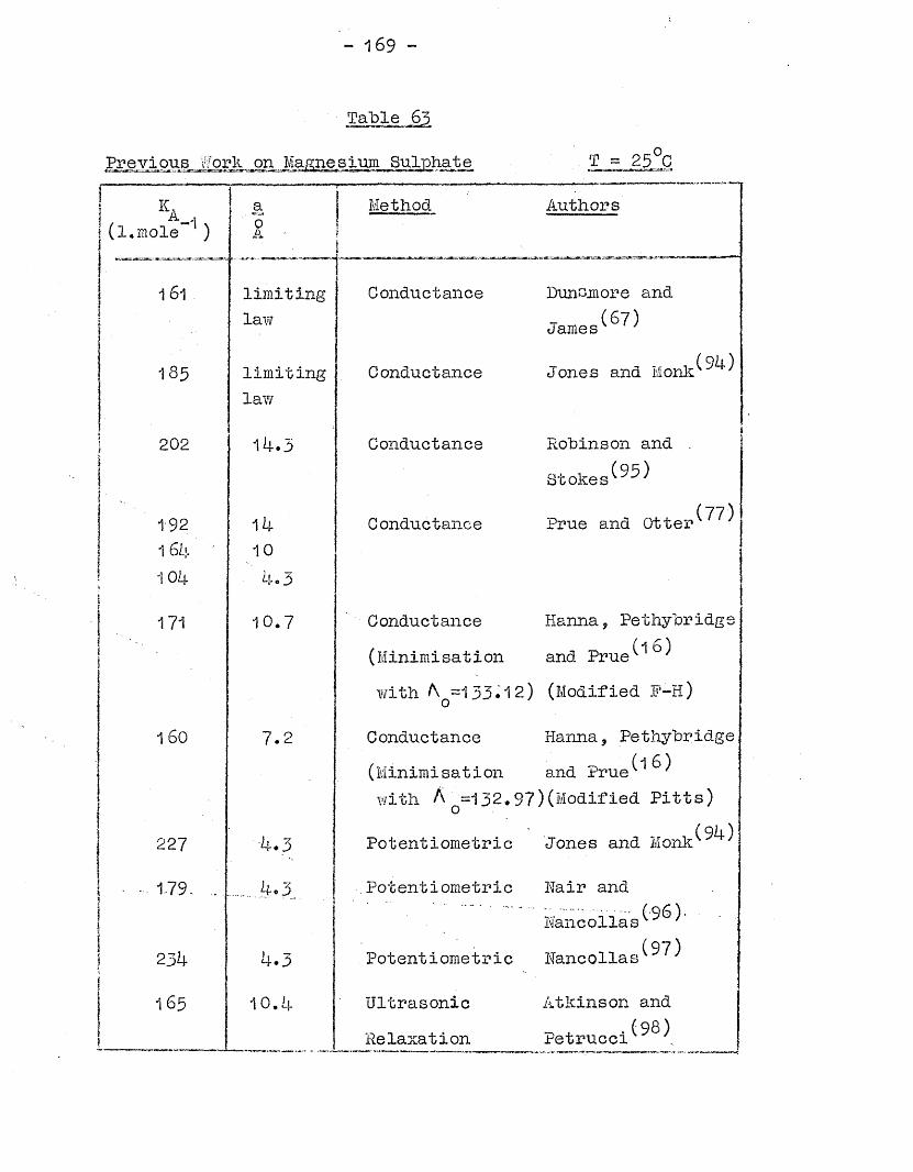
- 169 -

Table 65

Previous Work on Magnesium Sulphate T = 25°CJ| K.ij(l.mole )

aI .

j Methoditi

Authors

j _ _ _ _ _j 161 .i

limitinglaw

IConductance Dunumore and

T (67) James '

185 limitinglaw

Conductance Jones and Monk^“

202i 14.3 Conductance

iRohinson and . Stokes^"^

i ,I 1-92 1U Conductance (77)Prue and Otter| 1 64 10| 104 4.3i

171I •

10.7 Conductance(Minimisation

Hanna, Pethybridge and Prue^^

with =133.12) (Modified jj’-H)

160 7.2 Conductance(Minimisation with. A _=132.

Hanna, PethybridgeA T> (1 6 )and Prue /

97)(Modified Pitts)

227 4.3 Potentiometric (94)Jones and Monk

..179. . 4.3 .Potentiometric Hair andHancollas^^’i| 234j 1+.3 Potentiometric (97)Hancollasv

165 10.4 Ultrasonic Atkinson and! Relaxation Petrucci^^..

- 170 -

experimental data - that of Dunsrnore and James, However, the minimisations performed on this data hy Hanna, Pethybridge and Prue used only eleven of the thirteen original A/c points. The variety of technigues and models for evaluation of the data gives.rise to the wide scatter invalues of K; and a. The various experimental methods andevaluation technigues that were used "by the authors make direct comparisons difficult. Moreover, is strongly dependent on the value of a used to characterise thebehaviour of the free ions. The latter statement may befurther illustrated by reference to the analysis of the Dunsrnore and James data in the present work (Tables 8 and 9)

Manganese (il) SulphateThe results for manganese sulphate are shown in Table 6k

and the results of previous work are listed in Table 6b*Once again there is a wide scatter in the values of the parameters found in these investigations. The values found by Atkinson and Hallada and by Petrucci, Hemmes and Battistini are much lower than those obtained in the present work. This is probably due to the measurements of these authors being made on solutions more concentrated than those in this work. An analysis of these a u t h o r s * , results was made using the complete Pitts and Puoss-Hsia eguations with extrapolation function (3*17) * with a~values of 10 and 1l|. S. The results are shown in Table 66 from which it

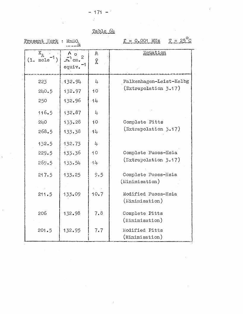
ka ■(l. mole ) 0 2cm. equiv. ^

a £ .

Equation

223 .132.94 4 Pa lkenhagen-Le i s t -Ke l“bg240.5 132.97 10 (Extrapolation 3.17)

250 132.96 14

11 6 .5 132.87 4

240 133.28 10 Complete Pitts268.5 133.38 14 (Extrapolation 3*17)

132.5 132.73 4229.5 133.36 10 Complete Fuoss-Hsia269.5 133.54 14 (Extrapolation 3.17)

217.5 133.25 9.5 Complete Fuoss-Hsia (Minimisation)

211.5 133.09 1 0 .7 Modified Fuoss-Hsia (Minimi sa t i on )

206 132.98 7.8 Complete Pitts (Minimisation)

201.5 132.95 7.7 Modified Pitts (Minimisation)

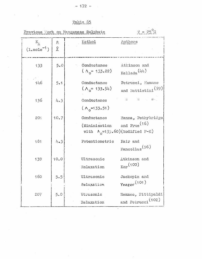
- 172 -

Table _6 5

Previous y-ork on Manganese Sulphate A3°fi

k almi*(l.mole" )

a£

Method 'Authors —— •

133 3.0 Conductance ( A 0= 133.22)

Atkinson and(kk)iiallada

Mi.6 5*1 Conductance ( A 0= 133.54)

Petrucci., Hemmes. .■(■•99) and hattistxni

136 A* 3 Conductance ( A 0=133.51 )

•• 11

201 10.7 Conductance(Minimisationwith A =133* 0

Hanna, Pethybridgeand Prue

60)(Modified P-Il)

1 81 ^•3 Potentiometric hair and Hancollas^^

139 1 0 .0 UltrasonicRelaxation

Atkinson andT, (100)Kor

1 60f3.3 Ultrasonic

RelaxationJackopin and Yeager^10|^

207 3.0 utrasonic Relaxation

Hemmes, Fittipaldi* -D - ,(102)and Pe'Gruec-L

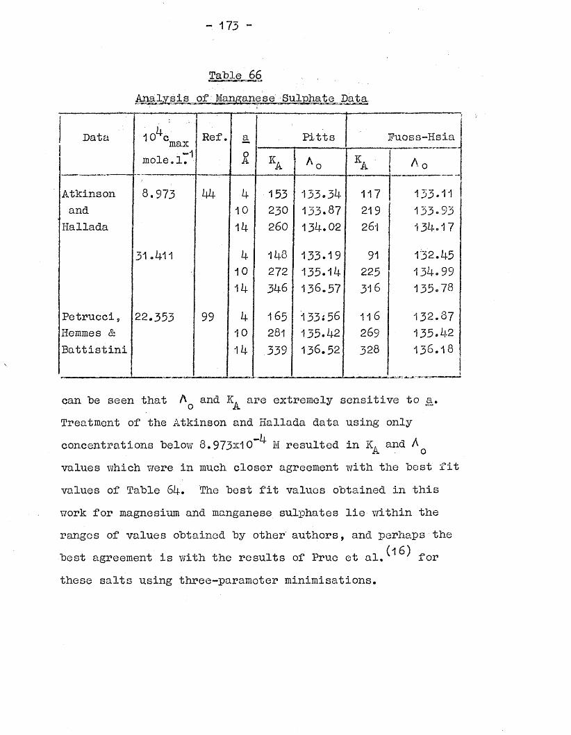
- 173 ~

Table 66Analysis of Manganese Sulphate Data

I

I Data 1 (Acmax Ref. a Pitts'

Fuoss-Hsiamole.l.^ & ka A 0 V A 0

Atkinson 8.973 44 k 153 133.34 117 133.11and 10 230 133.87 219 133.93Hallada 14 260 134.02 261 134.17

31 .411 k 11*8 133.19 91 132.4510 272 135.14 225 134.9914 346 136.57 316 135.78

Petrucci, 22.333 99 4 165 133*56 116 132.87Hemmes & 10 281 135.42 269 135.42Battistini 14 339 136.52 328 13 6.18

can be seen that Aq and are extremely sensitive to a.Treatment of the Atkinson and Hallada data using onlyconcentrations below 8.973 :10~^ M resulted in andvalues which were in much closer agreement with the best fitvalues of Table 64. The best fit values obtained in thiswork for magnesium and manganese sulphates lie within theranges of values obtained by other authors, and perhaps the

(1 6)best agreement is with the results of Prue et al, 7 for these salts using three-parameter minimisations.

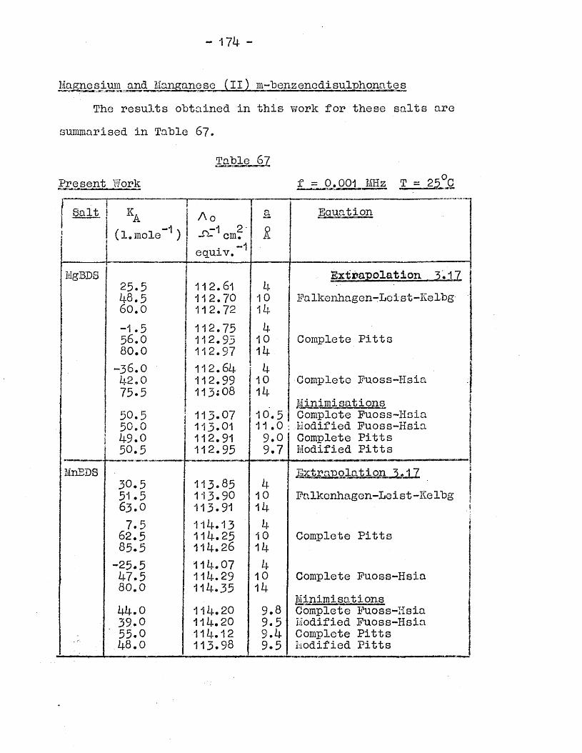
- m -

Magnesium and M a n g a n e s e ( I I ) m-benzenedisulphonatesThe resu3.ts obtained in this work for these salts are

summarised in Table 67*

Present Work f = 0,001 MHz T = 25°C

j Salt ji

kai —1 j (l.mole )t *

AofV-1 2-—- cm.

. -1equiv..

aI

“ ion

MgBDS Extrapolation 3.1725.5 112.61 448.5 1 1 2 .7 0 10 Fa lkenhagen-Le i s t-Ke 1-bg60.0 112 .7 2 14

-1.5 1 1 2 .7 5 45 6 .0 112.95 10 Complete Pitts80.0 112.97 14-3 6 .0 112.64 442.0 112.99 10 Complete Fuoss-Hsia75.5 11 3; 08 14 Minimisations50.5 113-07 1 0 .5 Complete Fuoss-Hsia5 0 .0 113.01 1 1 .0 Modified Fuoss-Hsia

i 49.0 112.91 9.0 Complete Pitts50.5 112.95 9.7 Modified Pitts

MnBDS Extrapolation 3*17 j30.5 113.85 451.5 113.90 10 Falkenhagen-Leist-Kelbg ]6 3.O 113.91 14 i

7.5 114.13 4 :

62.5 114.25 10 Complete Pitts85.5 1 1 4 .2 6 14-25.5 114.07 447.5 114.29 10 Complete Fuoss-Hsia80.0 114.35 14 Minimisations44.0 114.20 9.8 Complete Fuoss-Hsia39.0 114.20 9.5 Modified Fuoss-Hsia55.0 114 .12 9.4 Complete Pitts4 8 .0 113.98 9.5 Modified Pitts

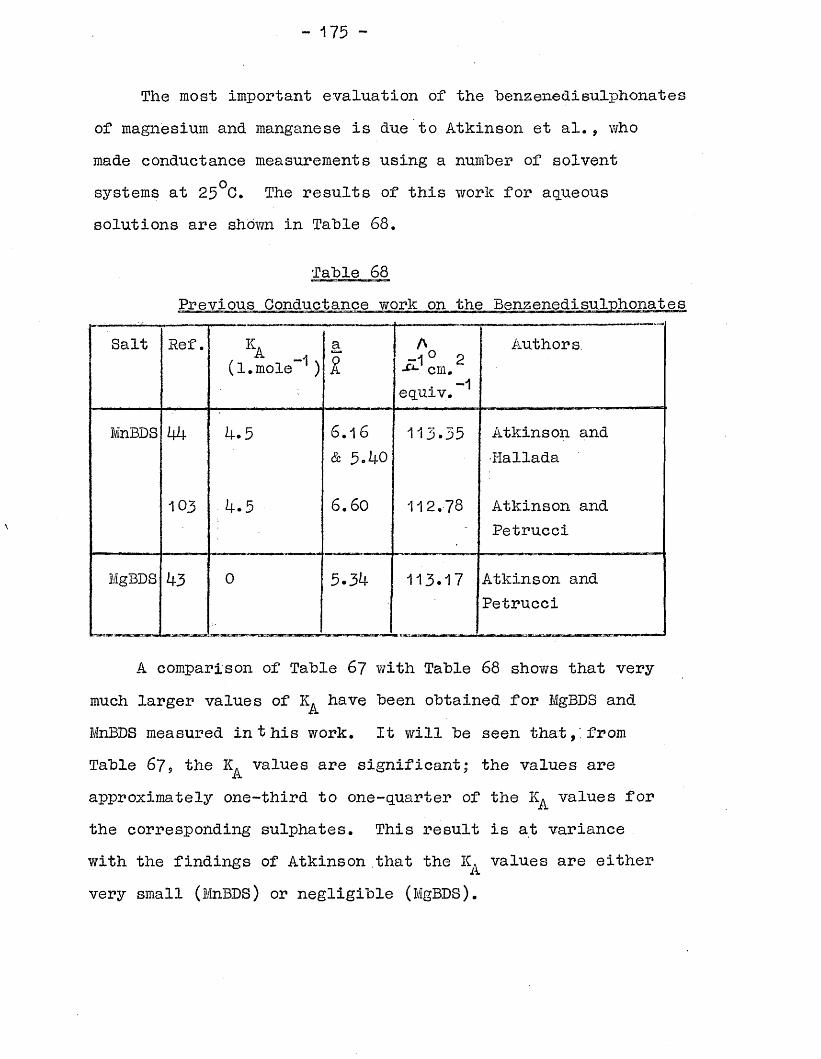
- 175 -

The most important evaluation of the benzenedisulphonates of magnesium and manganese is due to Atkinson et al., who made conductance measurements using a number of solvent systems at 23°C. The results of this work for aqueous solutions are shown in Table 68.

Table 68

Salt Ref. KA , (l.mole )a£

A-1 0 2cm.

. -1 equiv.

Authors.

MnBDS 44 4.5 6 .1 6

& 3.40113.35 Atkinson and

•Hallada

103 ■4.5 6 .6 0 112.78 Atkinson and Petrucci

MgBDS 43 0 5.34 113.17 Atkinson and Petrucci

A comparison of Table 67 with Table 68 shows that very much larger values of have been obtained for MgBDS and MnBDS measured in t his work. It will be seen that,', from Table 67, the values are significant; the values are approximately one-third to one-quarter of the values for the corresponding sulphates. This result is at variance with the findings of Atkinson that the IC values are either very small (MnBDS) or negligible (MgEDS).

- 176 -

The results of the present Y/ork also differ from those ofTahle 68 in the values assigned to A q and a. Atkinson* svalues of a are in most cases approximately one-half ofthe values found "by minimisation. This large differencemay be due to his use of the Fuoss-Gnsager equation^^v/hich Y/as only complete in terms up to pov/ers of c. Thedata of Table 68 Y/as reanalysed by the extrapolationfunction (3.17) using the complete Fuoss-Hsia and Pittsequations (v/hich have terms complete to and witha-values of k9 10 and 1 k i?. The results of this analysisare shown in Table 6 9. The values of and K, obtainedo nY/hen the concentration range v/as restricted ( to correspond to |(a = 0.2) are in much closer accord v/ith the results of extrapolation in the present v/ork (Table 12).

An examination of the results obtained by minimisation (Tables 13 and 16) shov/s that the a parameter values are dependent on the theoretical equation used to fit the data. Since a is so dependent on the free ion model, it is considered that speculation as to the cation - anion configuration for the ortho-, meta-, and para- isomers of the benzenedisulphonates^from conductance data v/ould yield little significant information at the present time.

It is concluded that the findings of Atkinson and co-Y/orkers, that the 2:2 benzenedisulphonates could be treated as essentially unassociated, are not confirmed for MgBDS and MnBDS by the measurements and analyses of the

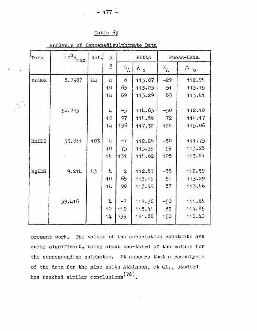
- 177 -

Data 10^Cmax Ref. Hr&

1—Pitts

---- — ----- {Fuoss-Hsia.

^ 0 ka ft 0

MnBDS 8.7987 44 4 6 113.07 -29 112.9410 65 113.25 51 113.1514 89 113.29 85 113.41

50,225 4 -5 114.63 -50 11 2 .1 0

10 97 114.56 72 114.1714 196 117.32 128 1 1 5 .0 6

MnBDS 35.811 103 4 -7 112 .26 -50 111.7510 75 113.39 59 11 3 .2 8

14 131 114 .62 105 113.81

MgBDS 9.214 43 4 2 112.83 -35 112.5910 65 113.19 51 113.2914 90 113.29 87 1 1 3 .4 6

59.416 4 -7 1 1 2 .3 6 -50 1 1 1 .6 410 119 115.41 83 114.8514 239 121.86 150 116,40

present work. The values of the association constants are ouite significant* heing about one-third of the values for the corresponding sulphates. It appears that a reanalysis of the data for the nine salts Atkinson* et al., studied

/ ~7Q \has reached similar conclusion's ,

- 178 -

The Murphy-Cohen EquationThe audio-frequency data obtained in this work were

also tested using the equation of Murphy and Cohen(17)(equation 1*12), as formulated in the original paper

Treatment of the data by extrapolation function 3*17yielded association constants that were more than doublethe values obtained by any of the other equations used.Moreover, A values were obtained that were relativelylow, compared to the previous results. As a check on thesuitability of the extrapolation method with this equation ..

(71 )the extrapolation techniques of Fuoss-KrausN J and (73 )Shedlovskyv were employed using the Murphy-Cohen equation*

A selection of the results obtained is shown in Table 70 for MnSO4 and MgBDS with a values of 8, 10, 12 and i4&-

Although there are differences between the extrapolation techniques employed, the values are all very high and f\ Q values too low, in comparison with the evaluation of this data by other equations.

When minimisations were.performed-with the Murphy-Cohen equation it was found that sharp minima were obtained yielding good degrees of fit between experimental and /calculated conductances. However, in all cases it was foundI that a good fit Y/as only obtained when the resultant values / of Ka were too high and A_ and a. were too small.

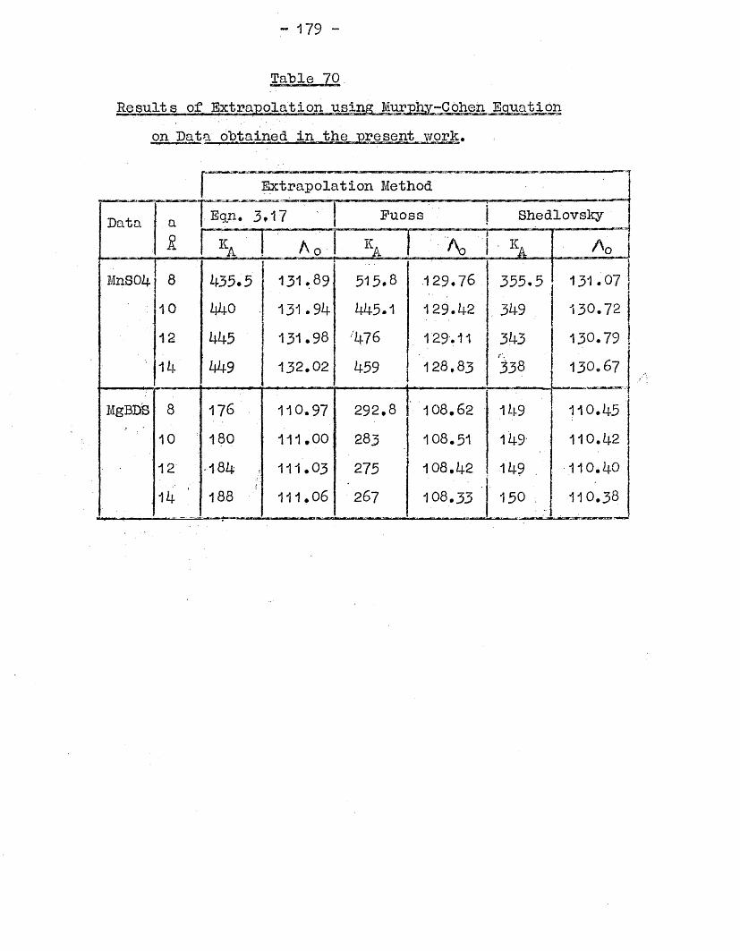
- 179 -

using Murphy-Cohen Equationon Data obtained in the present work*

Extrapolation Method

Data a Eqn. 3.17 Fuoss Shedlovsky. ----- . ------

R V A o ka ! Ac ' ka A 0 \

MnSOZf 8 435.5 131.89 515.8 129.76 355.5 131.0710 440 131.94 445.1 129.42 349 130.7212 445 131.98 '476 129.11 343 130.7914 449 132.02 459 128.83 338 130.67

MgBDiS 8 176 110.97 292.8 108.62 149 110.4510 180 111.00 283 108.51 149 11 0 .4 2

12 •184 ; 111.03 275 108 .42 149 . 1 1 0 .4 0

14 188 111.06 267 108.33 150 , 110.38

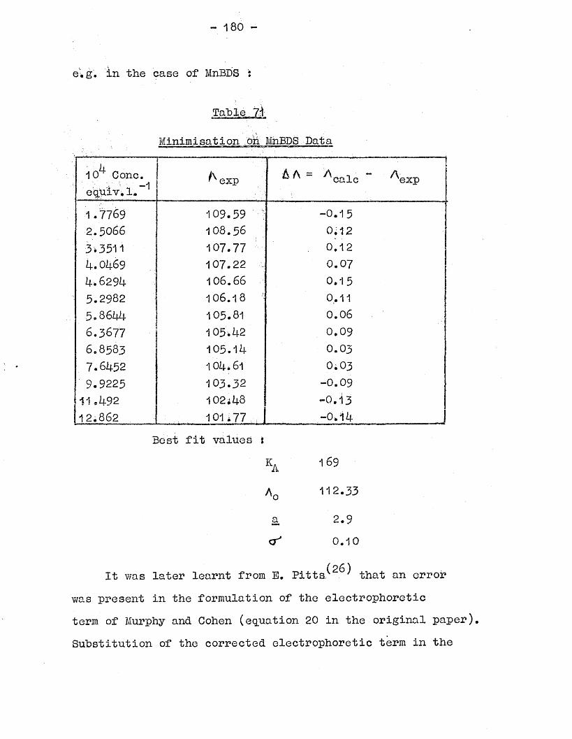
- 180 -

elg. in the case of MnBDS :

Table 7rl

Minimisation ,oh MnBDS Data

10^ Cone, equrv. 1.

r---------- -^exp

■’ ' | & A - A ca^c - ^exp

1.7769 109.59 - -0.152.5066 1 0 8 ,5 6 0,12

3.3511 1 0 7 .7 7 0.12k.0k69 1 0 7 ,2 2 . 0.07k>629k 10 6 .6 6 0.155.2982 106 .1 8 0.115 „ 86i+lf- 105.81 0.066.3677 1 0 5 ^ 2 0.096.8583 105.1 j+ 0 .0 3

7.6IJ.52 1 oil, 61 0;039.9225 1 0 3 .3 2 -0.09

1 1eh92 10 2jl+8 -0.1312 .86 2 101.77 I “0.1^

Best fit values iKa 169

A0 112.33

a 2.9cr o.io

It was later learnt from E. Pitts^2^ that an error was present in the formulation of the electrophoretic term of Murphy and Cohen (equation 20 in the original paper). Substitution of the corrected electrophoretic term in the

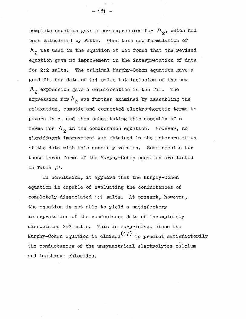
- 1 8 1 -

complete equation gave a nev/ expression for Ag*-which had been Calculated by Pitts. When this new formulation of Ag was used in the equation it was found that the revised equation gave no improvement in the interpretation of data for 2:2 salts. The original Murphy-Cohen equation gave a good fit for data of 1:1 salts but inclusion of the new A 2 expression gave a deterioration in the fit. The expression for was further examined by assembling the relaxation, osmotic and corrected electrophoretic terms to powers in c, and then substituting this assembly of c terms for h in the conductance equation. However, no significant improvement was obtained in the interpretation of the data with this assembly version. Some results for these three forms of the Murphy-Cohen equation are listed in Table 72.

In conclusion, it appears that the Murphy-Cohenequation is capable of evaluating the conductances ofcompletely dissociated 1:1 salts. At present, however,the equation is not able to yield a satisfactoryinterpretation of the conductance data of incompletelydissociated 2:2 salts. This is surprising, since the

(1 7)Murphy-Cohen equation is.claimed' to predict satisfactorily the conductances of the unsymmetrical electrolytes calcium and lanthanum chlorides.

- 182 -

Interpretation of 1; 1

N.B, Equn. 1 Equn. 2

Equn. 3

1) Potassium Chloride(Data of Owen and keldcs^

a = 3*03 £ A 0 = 1'+9.9210^ Cone.

Mole I.-"'1— :.'.iini.— .... i i-------

^ exp AA = A - /\calc expEqun. 1 Equn. 2 Equn. 3

. 5.506 1U7-7U -0.01 0.11 0.03■i 5.636 1 i|6.26 0.00 0.33 0.2631.bOk 144.35 0.03 O.83 0.72~7C\ &&X 11±2.49 0.08

______1.55 1 .38

(17 )= Murphy-Cohen Equation' y = Original equation with recalculated by Pitts.

= Original equation with A in assembly version

2) Magnesium Sulphate / £T"7 \(Data of Dunsmore and James )

0 ~ 8 I a = 10 £ a = 1/4. £K,A Ao K, f o K',ii. (\q

Equn, 1 372 131. 69 376 131.72 381+ 131.78Equn, 2 383 131.77 387 131.80 395 131.86Equn. 3 387 131.76 j 389 131.82 39b 131.86

-------------- ----

- 183 -

(ii) Radio-Frequency ResultsThe dispersion of equivalent conductance of aqueous

solutions of magnesium and manganese (II) sulphates andbenzenedisulphonates has been measured for concentrations

- i i - 3 - iin the range 1.5x10 to 1,5x10 eauiv. 1. and atfrequencies between 1 and 50 MHz. The experimental results{(\% ) are shown in Tables 17 to 60, together with theexp,

theoretical percentage dispersions as calculated from the Falkenhagen-Leist-Kelbg equation equation (1.32),and the dispersion due to relaxation of the free ions - ion-pair equilibrium as calculated from the Gilkerson equation (1,38), Also shown are the values of A / j>otal given by :

A %otal = (ASS’LK^1'32 + °/jGilkerson^1 *38)..........(3.23)

The effects of ion-pair and ion atmosphere relaxations are taken to be additive and these quantities are compared with the experimentally measured conductance dispersions in Figures 3.7 to 3.1A.

The results of applying extrapolation techniques to the data for K, and A are also included in Tables 17 to 60.ii. OThe extrapolations have been applied using the Falkenhagen- Leist-Kelbg equation (1.5) cukl the Fuoss-Hsia equation plus additional ion atmosphere relaxation terms (3.21). The values of K. and A obtained are listed for a parameteril Ovalues of k9 10 and li+ n. The Falkenhagen-Leist-Kelbg

equation predicts relatively small changes in and Awith a, compared to the results using equation ( 3.21 ).Finally, the results of three-parameter minimisations forK., A and a are shown at the bottom of each table. For A o —frequencies in the range 1 to 5 MHz, where the ion-pair relaxation effect was negligible, equation (3.21) was used to calculate conductances for the minimisations. For frequencies of 10 MHz and above, the Gilkerson term was included to give an equation of the form :

A = (A 0- A A e)0+AVx)/(l+3^/2) + Rel.0<00l- Rel.f + AG .................... (3.2A)

where A 0- is the increase in conductance as calculated by the Gilkerson equation.

In general, the errors associated with radio-frequency conductance determinations were much greater than those associated with the audio-frequency measurements. The standard deviations of the extrapolation plots gave variations of the order of 0.2 % in A and 0.5-1.0 % in K,. However, considering the relatively poor precision of

.li.

the radio-frequency conductances, a reasonable fit (expressed as d ) was obtained between experimental conductances and equations (3*21 ) and (3.24) which are only first approximations to high-frequency conductance equations.In these equations the frequency dependent relaxation term has only been included up to powers of c2

- 185 -

and higher cross terms have not "been derived.Inspection of the minimising parameters for each

electrolyte over the frequency range studied showed noapparent trends in a and A with frequency. Theidentification of the a parameter values with approximately10 £ is noteworthy, however, since this order of magnitudecorresponds to the Eigen distance. The values of theassociation constants obtained appear to sho?/ some- dependenceon frequency and the minimising values for each electrolyteat each frequency used are summarised in Table 73? togetherwith their associated a and A values. K. values are“ o Aplotted against the frequency for each electrolyte in Figures 3.15 to 3.1 8. For all four electrolytes studied,

decreases above a certain frequency up to 50 MHz, the highest frequency of measurement. The values for magnesium sulphate and benzenedisuiphonate decrease above 5-10 MHz, whereas the values for the manganese salts only decrease above about 20 MHz* In all cases the frequency at which a decrease in is apparent is close to the frequency where the magnitude of the G-ilkerson expression for ion-pair relaxation becomes significant.

Figures 3*7 to 3*14 compare the experimentally measured dispersions for the four electrolytes studied with the dispersion predictions of the Falkenhagen-Leist-Kelbg equation (A %-^j^ “ solid lines) and with the total dispersion

- dotted lines). The minimising values of ,

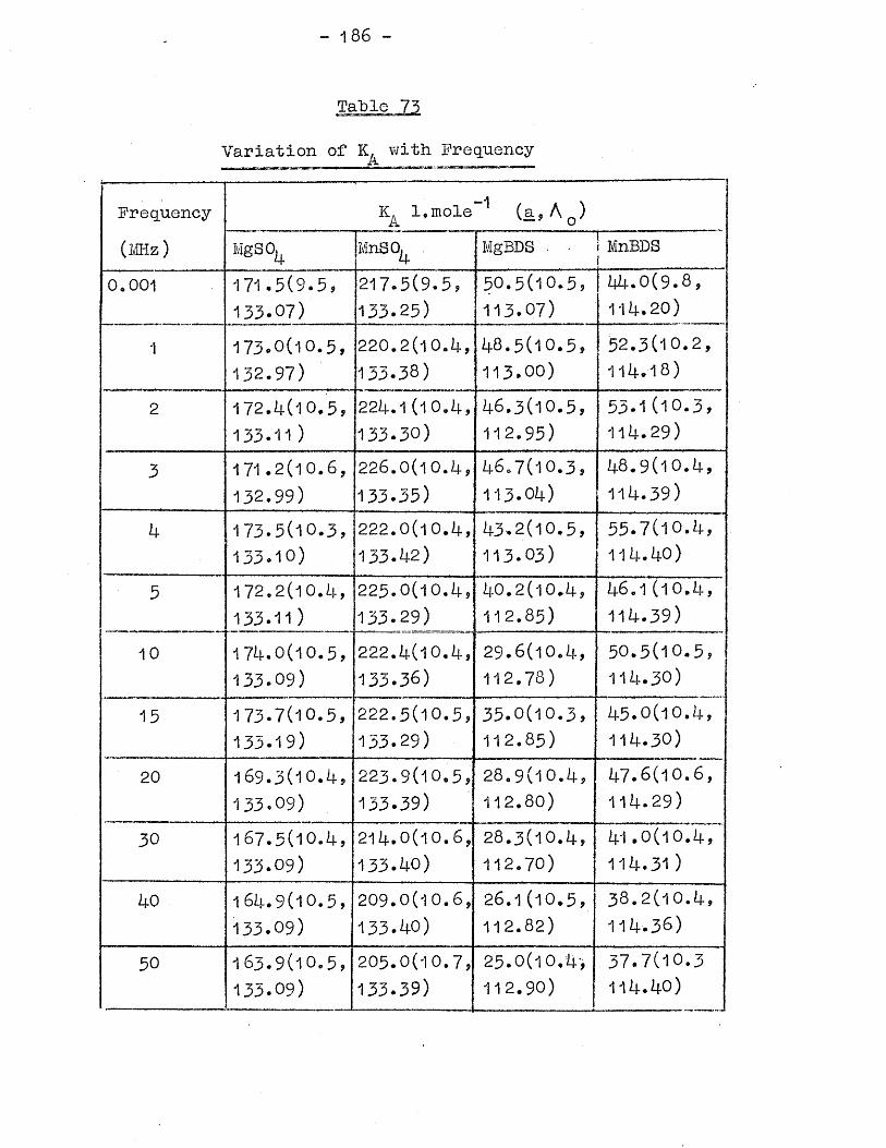
- 186 -

Table 75

Variation of with Frequency

Frequency (MHz )

l.mole (a»A0)MgSO. MnSQ^ MgBDS - I MnBDSi

0.001 171.5(9.5, 133.07)

217.5(9.5 ,133.2 5)

5 0.5 (1 0.5 ,1 1 3.0 7)

44.0(9.8,114.20)

1 173.0(10.5,132.97)

220.2 (1 0.4 ,133.3 8)

48.5(10.5,113.00)

52.3(10.2,114.18)

2 172.4(10.5, 133-11)

224.1 (1 0.4 , 1 3 3.3 0)

46.3(10.5,112.95)

53-1 (10.3, 114.29)

3 171.2(10.6, 132.99)

226.0(1 0.4 ,1 3 3.3 5)

46.7(10.3,113.04)

48.9(10.4,114.39)

4 173.5(10.3,133.10)

222.0 (1 0.4 ,133.4 2)

43.2(10.5,113.03)

55.7(10.4,114.40)

5 172.2(10.4, 133.11)

2 2 5.0(1 0.4 ,1 3 3.2 9)

40.2(10.4,112.85)

46.1 (10.4, 114.39)

10 174.0(10.5,133-09)

222.4 (1 0.4 ,1 3 3.3 6)

29.6(10.4,112.78)

50.5(10.5,114.30)

15 173.7(10.5,135.19)

2 2 2.5 (1 0.5 ,1 3 3.2 9)

35.0(10.3,112.85)

45.0(10.4,114.30)

20 169.3(10.4,133.09)

2 2 3.9(1 0.5 ,133.3 9)

28.9(10.4,112.80)

47.6(10.6,114.29)

30 167.5(10.4,133.09)

214.0 (1 0.6 ,1 3 3.4 0)

28.3(10.4,112.7 0)

41.0(10.4, 114.31)

40 1 6 4.9(10.5 ,133.09)

209.0 (1 0.6 ,1 3 3.4 0)

26.1 (10.5, 112.82)

38.2(10.4, 114.36)

50 1 6 3.9 (1 0.5 ,133.09)

205.0(1 0.7 ,133.3 9)

25.0(10.4',112.9 0)

37.7(10.3114.40)

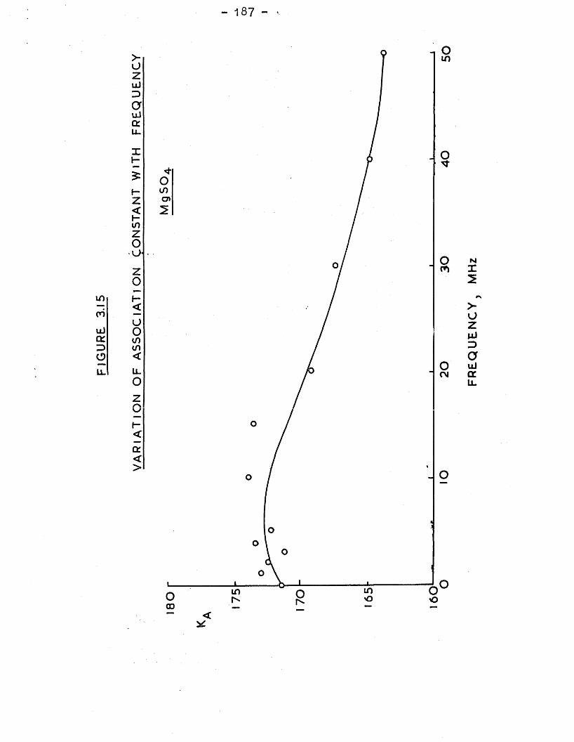
- 187 -

in<nuJccz>oLL

>•uzuJ3au i<Xu_Xh-

HZ<h*inzOazO<Uoinin<Ll

OA

<a<>

mC7>

OJ

in o

FR

EQ

UE

NC

Y,

MH

z

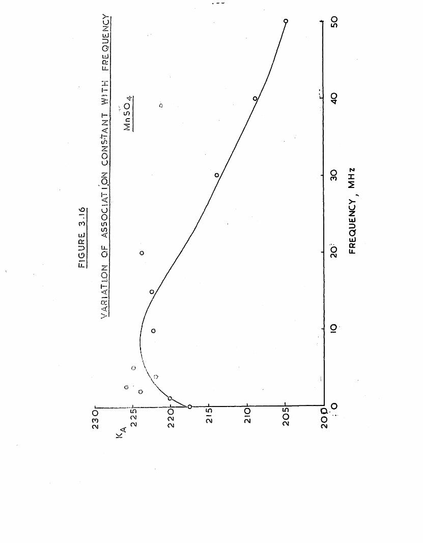
FIG

URE

3.16

in

Ll,

CM

in amCM CM

FRE

QU

EN

CYt

MH

z

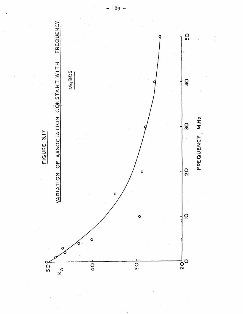
- 189 -

in

O

ro

n

FR

EQ

UE

NC

Y,

MH

z

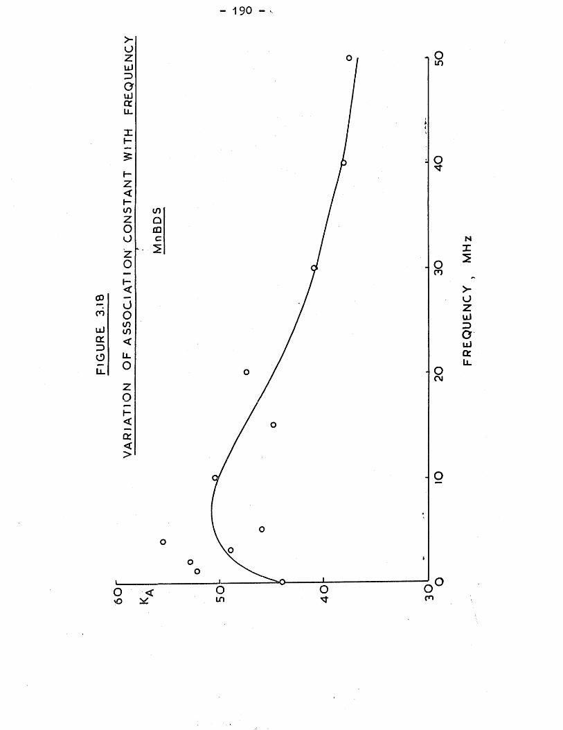
- 190 -

L l

CO

rouJCtZDOLl - OOJ

min

FRE

QU

EN

CY

,

MH

z

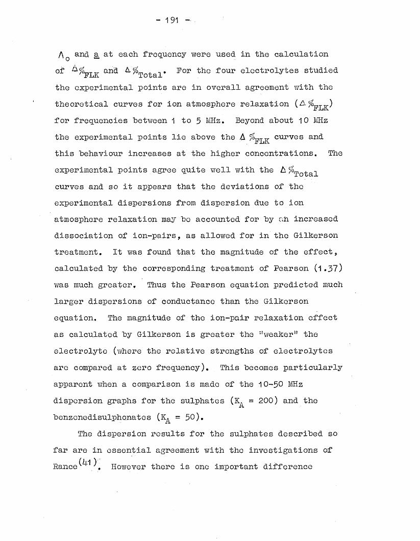
-191 -

A and a at each frequency were used in the calculation

oi ^ L K and ^^Total* ^0J} four studiedthe experimental points are in overall agreement with thetheoretical curves for ion atmosphere relaxationfor frequencies between 1 to 5 MHz. Beyond about 10 MHzthe experimental points lie above the A curves andthis behaviour increases at the higher concentrations. Theexperimental points agree quite well with the A potalcurves and so it appears that the deviations of theexperimental dispersions from dispersion due to ionatmosphere relaxation ma3r be accounted for by ah increaseddissociation of ion-pairs, as allowed for in the Gilkersontreatment. It was found that the magnitude of the effect,calculated by the corresponding treatment of Pearson (1.37)was much greater. Thus the Pearson equation predicted muchlarger dispersions of conductance than the Gilkersonequation. The magnitude of the ion-pair relaxation effectas calculated by Gilkerson is greater the ;?weaker5J theelectrolyte (where the relative strengths of electrolytesare compared at zero frequency). This becomes particularlyapparent v/hen a comparison is made of the 10-50 MHzdispersion graphs for the sulphates (K = 200) and thebenzenedisulphonates (K = 5 0).

The dispersion results for the sulphates described so far are in essential agreement with the investigations of Ranee^ However there is one important difference

- 192 -

between the results of the present work and those of Ranee and this concerns the manganese sulphate dispersion maximum previously found. It was noted in Part I that Ranee had observed a dispersion maximum for manganese sulphate between 2-3 MHz which could not be explained by the Gilkerson theory. This maximum Y/as attributed to a resonance dehydration of the hexahydrated cations, resulting in increased mobility and hence conductance at these frequencies. An absorption peak in the region of 3 to 5 MHz has been found from ultrasonic absorption work on manganese sulphate solutions^^5 106) this has beenidentified v/ith a desolvation step whose rate Y/as dependent on the rate of exchange of solvent molecules on the c a t i o n ^ H o w e v e r , the conductance technique used in the present v/ork has not shov/n a dispersion maximum; the present results can be explained in terms of ion atmosphere relaxation with additional account taken of the free ion - ion pair equilibrium.

Magnesium sulphate was.further examined in this context to see if any anomalous systematic dispersions could be observed. Conductances were determined at frequencies in the region of 0.1 MHz. This frequency was selected since an ultrasonic absorption peak has been determined in the region of 0*14 MHz for magnesium sulphate ? v/hich has again been identified v/ith desolvation. At a frequency of the order of 0.1 MHz, the Gilkerson term is effectively zero and the

- 193 -

calculated dispersion due to ion atmosphere relaxation (equation 1.32) is of the order of 0.01%. This dispersion represents the absolute limit of accuracy of the conductance measurements, based on the discrimination pf the bridge. Measurements were made at frequencies of 0.10, 0,12 and 0.1 A MHz for magnesium sulphate solutions in the concentration

-Ll -3range 10 to 10 M and in all cases no enhancements ofconductance were found over the corresponding audio-frequencyvalue i.e. A % =0. It is therefore concluded that theu ' exp.technique used in this work is not capable of determining enhanced dispersions due to desolvation processes for magnesium and manganese sulphates. Consequently no dispersion maxima have been found over the frequency range studied. The manganese sulphate maximum determined by Ranee was perhaps due to inconsistencies in the radio­frequency measurement technique since a specially constructed detector system was used rather than the SR268 oscillator- detector unit used throughout the present work.

In recent years much use has been made of the ultrasonic absorption technique to investigate the relaxation of ion- pair equilibria in aqueous solutions of bi-bivalent electrolytes. According to Eigen^^ the combination of oppositely charged free ions is hindered by hydration layers and cannot be treated as a one-step mechanism. It has to proceed stepwise and such a system has a spectrum of relaxation times in which the number of time-constants

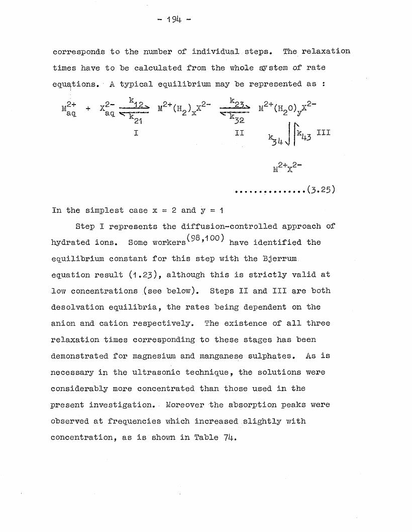
corresponds to the number of individual steps. The relaxation times have to be calculated from the whole system of rate equations, A typical equilibrium may be represented as :

In the simplest case x = 2 and y = 1Step I represents the diffusion-controlled approach of

equilibrium constant for this step with the Bjerrum equation result (1 .23 ), although this is strictly valid at low concentrations (see below). Steps II and III are both desolvation equilibria, the rates being dependent on the anion and cation respectively. The existence of all three relaxation times corresponding to these stages has been demonstrated for magnesium and manganese sulphates. As is necessary in the ultrasonic technique, the solutions were considerably more concentrated than those used in the present investigation. Moreover the absorption peaks were observed at frequencies which increased slightly v/ith concentration, as is shown in Table 74.

\I II

(3.25)

hydrated ions. Some workers have identified the

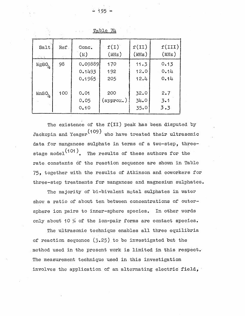
- 195 ~

Salti. •• ‘ v •

Ref. Gone.(M)

£(I)(MHz)

£(II)(MHz)

f(III) (MHz)

KgSO, 98 0.09889 170 11 .3 0.130.1493 192 12.0 0 .1 4o . i 965 205 12.4 0.14

MnSO, 100 0.01 200 3 2 .0 2.7L f .

0 .0 5 (approx.) 34.0 3 .10 .1 0 35.0 3.3

The existence of the f(ll) peak has been disputed by (1 09 )Jackopin and Yeager who have treated their ultrasonic

data for manganese sulphate in terms of a two-step, three- (101 )stage model . The results of these authors for the

rate, constants of the reaction sequence are shown in Table 75, together with the results of Atkinson and coworkers for three-step treatments for manganese and magnesium sulphates.

The majority of bi-bivalent metal sulphates in water show a ratio of about ten between concentrations of outer- sphere ion pairs to inner-sphere species. In other words only about 10 % of the ion-pair forms are contact species.

The ultrasonic technique enables all three equilibria of reaction sequence (3 *2 5).to be investigated but the method used in the present work is limited in this respectv The measurement technique used in this investigation involves the application of an alternating electric field,

Hate Constants, for ion Association .in m

( i ) MgSO,

Atkinson and Petrucci 8)

k12k21

M sec. ^ 00.CV] X 1010sec. 9.6 X 108

k23k32

sec."" CVJ• X 107sec.” 3.7 X 107

k3U sec.-1sec.

1 . u X 105

k43 8.0 X 105

(ii) MnSO,

1 o10 ^ 21°8 k21

M“1sec.

107 k23 sec.107 k32 sec.

105 k3^ sec.'105 k43 sec.

sec. - 1'

-1

Atkinson & Kor

-1 k.2

8.0

6.9

(100) Jackopin &

. -1

-1

(2 x 107) (2 x 107)

1.9

k.S 1..U

( $ Two-step mechanism) and the chemical eguilibrium to "be observed must involve a charge-rreduction process. The diffusion-controlled approach of the free ions to form a solvent-separated ion- pair can he detected. ‘ However * no such power loss will he

- 197 ~

measured for the ion-pair desolvation steps II and III inequation (3*25) since each of the ion-pair types isnon-c onduct ing.

It has heen possible to estimate the rate constantk^ for the dissociation of outer-sphere ion-pairs tofree ions by use of the Gilkerson equation (1.3&). In thisequation the rate constants k and k^ of (i•33) wereidentified with k^ and k 2 respectively. An estimate ofk^2 was made from the expression for the rate of ion

(27)recombination due to Onsager' ' :

ki2 = 1 .207TNzeAo .............. (3.26)FoD

where A is the limiting equivalent conductance of theions and F is the Faraday constant. The s parameter ofGilkerson was set equal to the Bjerrum q distance (1 .24).The Gilkerson term was then evaluated for various values of

and those values giving the best agreement betweenexperimental conductance increases and the theoreticalvalues cf A/on , 1 were used in the compilation of Tables lo-caj.17 to 60. The values of k0. giving the best fit to the experimental data were as follows :

MgSO. 1 x 10^ sec.’"'14 a -IMnSO. 9 x 10 sec.^ " 9 - 1 MgBDS 1 x 1 0 sec.

MnBDS 1 x 10^ sec.”"1

- 198 -

The agreement is satisfactory "between these results and the values for k^ in Table 75? considering the apprdximaticns involved in the calculations and the differences in the methods of determination. It was found that further simple estimates could "be made of the ion- paih equilibria by assuming a two-step mechanism for ion association :

M2+ + X2- -k-12*' m2+(hC)o)x2" — m2+x2-ag. ag -- 2 -----

(3-27)

For this scheme : (1 + K32) ...........(3.28)where IC. is the overall association constant for theAreaction and and are outer-sphere and inner-sphereassociation constants respectively (K^ = k / k ^ ;

IC_0 = k0_/k_n). This simple mechanism has been tested for 32 23 3 2(110 1 1 1)a number of benzenedisulphonates in methanolv 9 ' and

for some tetraalkylammonium salts in 1-butanol and (1 1 2)1-pentanolv . Estimates of K0. and K_n were made md\ 3d

the following way: was calculated fromk^2 was obtained from the Onsager equation (3 .26) and was

10 —1 —1of the order of ipdO l.mole sec. (i.e. k g wasassumed independent of the frequency of the applied field). k2.j was obtained from minimisation of the conductance data using equation (3 .2k) for the calculation of theoretical. <• conductances« A three-parameter minimisation program was used, with K ? a, and kg as the three variables.

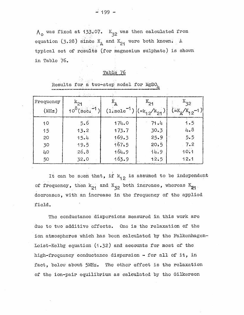
- 199 -

A was fixed at 133* 07 K_0 was' then calculated from 5^equation (3*28) since and K^ were hoth known; & typical set of results (for magnesium sulphate) is shown in Table 76*

Results for. a two-step model for MgSO^

Frequency(MHz)

*21j. nQ / ; . “*1 \10 (sec; ) —1(limole )

K21 (=1 2/k21 )

IC32^ V K12H)

10 5,6 17U.0 71.4 1.513 13.2 173.7 30.3 4.820 15. k 169.3 25.9 5.530 19.5 167.5 20.5 7.2ko 26.8 16i+i 9 14.9 10*150 3 2 .0 163.9 12.5 12.1

It can be seen that, if k 2 is afeSumed to be independent of frequency, then k^ and both increase, whereas decreases, with an increase in the frequency of the applied field.

The conductance dispersions measured in this work are due to two additive effects* One is the relaxation of the ion atmospheres which has been calculated by the Falkenhagen- Leist-Kelbg equation (1.32) and accounts for most of the high-frequency conductance dispersion - for all of it, in fact, below about 5MHz. The other effect is the relaxation of the ion-pair equilibrium as calculated by the Gilkerson

- 200 -

equation (1.38). The equation of Falkenhagen-Leist-Kelbgis, in a sense, the limiting lav/ for high-frequencyconductance, since frequency corrections have only been

±applied to the c2 terms and higher terms in c have notbeen derived. It was noted in Part I that a rigorousderivation of either a Pitts or Fuoss-Hsia equation for useat high frequencies would he an extremely difficult task.In this work a high-frequency conductance equation has heenused (3.21) which combines the Fuoss-Hsia complete equationand an incremental relaxation term as calculated byFalkenhagen, Leist and Kelbg. This equation is only anapproximation to a complete solution of high-frequencyconductivity but it represents an improvement on theoriginal Falkenhagen-Leist-Kelbg equation (1.3)> since thecomponents of the equation that are frequency independent

3/2have been evaluated up to terms in c ' .

PART IV SECTION 1

C ON CULSIONS

- 202 -

(1) The conductances of aqueous solutions of magnesium and manganese (II) sulphates and benzenedisulphonates have been measured at frequencies from 1 KHz to 50 MHz -using an audio-frequency Wheatstone bridge and Wayne-Kerr B201 and B801 radio-frequency bridges.

(2) A relative method, using potassium chloride as a reference electrolyte, has been used for tie measurement of the radio'-frequency conductances ( 1 to 50 MHz). This does not rely on the calibration of the bridge.

(3) The following conductance equations were used in thiswork for the evaluation of audio-frequency conductance data;the Falkenhagen-Leist-Kelbg equation^\ the complete andmodified forms of the Pitts^9"*^ and Fuoss-Hsia^^ * 5-)

(17)equations and the Murphy-Cohen equation' . These equations have been treated as three-parameter equations in terms of K , the ion-pair association constant, a the closest distance of approach of free ions, and (\q9 the conductance at infinite dilution.

The numerical predictions from the conductance equations have been compared for the case of a model 2:2 salt. It was noted that there were significant differences between the complete and modified Pitts equations and the Fuoss-Hsia equations. The effect of the variation of a on the equivalent conductance A was investigated for these

- 203 -

equations. It was found that the PaIkenhagen-Lei s t-Kelhg equation gave A values that were much less affected by changes in £ than any of the other equations*

(b) ‘The various methods available for the computation of 9 a ? an& A from audio-frequency conductance data haveA O

been reviewed. These methods were divided into the two classes : extrapolation, and minimisation.

(5) An extrapolation technique was described (3*17) whichhas been used in this work with the Falkenhagen-Leist-Kelbg,and complete forms of the Pitts and Fuoss-Hsia equations.The numerical values of K, and A were found to be dependentA oupon the value assigned to the a parameter and the theoretical equation used to describe the behaviour of the completely dissociated electrolyte. The Falkenhagen-Leist-Kelbg equation predicted values of K. and A that were relativelyA Oinsensitive to variations in a. It is suggested that the most satisfactory means of expressing the characteristic parameters of an electrolyte is always to quote K , A and a.

(6) Computer programs have been written for minimisationmethods to evaluate K,, A and a from the conductance data,a o — ‘It was found that the Falkenhagen-Leist-Kelbg equation was unsuitable for the minimisations on data obtained in this

- 2 04 -

work, The audio-frequency data were tested using the complete and modified Pitts and Fuoss-Hsia equations, and the radio-frequency data was examined using the complete Fuoss-Hsia equation with additional relaxation terms to take account of ion atmosphere relaxation effects (3-21),

(7) The results of minimisations on the audio-frequency data showed that the two forms of the Pitts equation yielded smaller A and a values than those obtained using theo —

Fuoss-Hsia equation. The differences between the complete and modified forms of these two equations, in terms of their minimising parameters, were very small.

(8) The values of the association constants, A 0 an< a values obtained in this work for magnesium and manganese sulphates were in overall agreement with the results of other workers.

(9) The findings of Atkinson et al., that manganese and magnesium benzenedisulphonates could be treated as essentially unassociated, is not confirmed by the measurements and analyses of the present work. The values of the association constants have been found to be about one third of the values of the corresponding sulphates.

- 205 -

(10) The equation of Murphy and Cohen is capable of evaluating conductances of completely dissociated 1:1 salts, fiov/ever it has been found that this equation is not able to yidld a satisfactory interpretation of the conductance data for incompletely dissociated 2:2 salts. Treatment of the audio-frequency data by minimisation yielded K^ values that were more than double the values obtained by any other equation used, and the corresponding values of A 0 and a were found to be very small* The use of a revised equation as suggested by Pitts^^ gave no improvement in the interpretation of the data*

(11) The radio-frequency conductance data were treated by extrapolation using the Palkenhagen-Leist-ICelbg equation and equation (3*21). Minimisations were performed using equations (3.21) and (3.24).

(12) The increases in conductance brought about by thehigh-frequency field could be explained in terms of ionatmosphere relaxation plus the effect of the relaxation of

( 0 the ion-pair equilibrium as calculated by Gilkerson *All four electrolytes studied showed variations in K^ values with frequency. These variations can be attributed to the relaxation of the ion-pair equilibrium. Rate constants for the rate of ion-pair dissociation have been estimated according to the Gilkerson theory, using the Onsager expression for the rate of free ion recombination.

- 206 -

(13) The conductance dispersion maximum at 2 - 3 MHz for manganese sulphate that Ranee observed^ has not heen found in the present work. It is suggested that this result of Ranee was due to inconsistencies in the measurement apparatus then used.

PART IV SECTION 2

APPENDICES

- 208 -

APPENDIX 1 Example of Minimisation Program

The following is an example of the type cf minimisation program used in this work. The program was written in Algol for an ICL 1905F computer and it minimises the experimental conductance data with respect to the modified Pitts equation. The data is read in as N pairs of Oj/A i values. The three parameters > A 0 an& a a3?e varied over the following preselected ranges: runs from value KA toKAMAX in steps of DM, A 0 runs from L0 to LOMAX in steps of DLO, and a is given a series of M values. Input is required in the f oilowing order :

ETA (viscosity of solvent)D (dielectric constant of solvent)T (temperature)Z (valency of symmetrical electrolyte under investigation)L0 (starting A value)ICA ( starting K. value)DLO DICA . .LOMAXKAMAXM (number of a values)N (number of c^/A j pairs)AR[A] (M a values)C(l,Jl (N pairs of c and A values)

The output consists of the sum of the squared deviationsbetween calculated and experimental conductances and thecorresponding K , A and a.

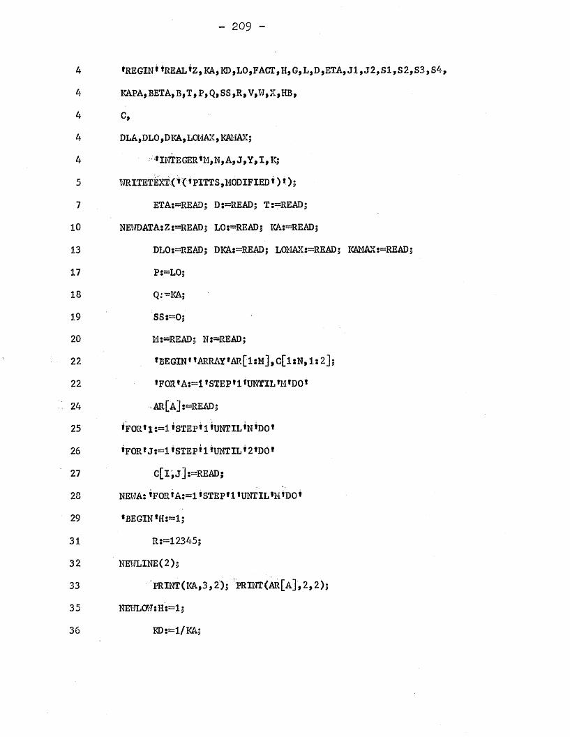
- 209 -

4 ’REGIN’’REAL’Z,KA,KD,L0,FACT,H,G,L,D,ETA, J1,J2,SI,S2,S3,S4,

4 KAPA,BETA,B,T,P,Q,SS,R,V,W,X,HB,

4 C,4 DLA,DL0,DKA,LOMAX, KAMAX;

4 »im,EGER»M,N,A,J,Y,I,K;5 WRITETEXT<’ PITTS,MODIFIED * ) ’ ) I7 ETA:~READ; D:=READ; T:=READ;10 NEWDATA:Z:=READ; LO:=READ; KA:=READ;13 DLO:=READ; DKAs=READ; LOMAX:=READ; KAMAX s==READ;

17 Pj=LO;18 Q:-KA;

19 SS:=0;20 M:=READ; N:=READ;22 ’BEGIN*’ARRAY*AR[12M],C[1:N,1s2];

22 ’FOR * A:=l’ STE P ’ 1 ’UNTIL ’M ’DO ’

24 AR[A]:=READ;25 ’FOR’1:=1’STEP’1’UNTIL ’N ’DO’26 ’FOR * Js=l’STEP «1 ’UNTIL * 2 ’DO *27 c[l,j]:=READ;28 NEUA: ’F0R’A:=1’STEP’l’UNTIL’M ’DO’

29 «BEGIN«Hj=1;31 Rr=12345;32 NEULINE(2);33 PRINT ( KA, 3,2); PRINT(AR[a ],2,2);

35 NEULOtt:H:=l;36 KD:=1/KA;

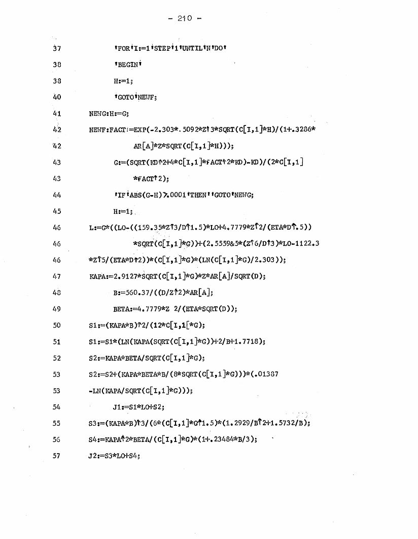
- 210 -

37 *F0R»I:=1*STEP»1 *UNTIL»N *D0»

38 *BEGIN*38 H:=l|40 1G0T0»NEWF$41 NEl"JG:H:==G542 NEWF:FACT: =EXP(-2*303*. 5092*Zt 3*SQRT(C[l,l]*H)/(1+.3286*

42 AR[A]*Z*SQRT(c[l, 1 ]*H) ) >543 G:=(SQRT (KDf 2+4*C[l, 1 ]*f ACTf 2*KD )~KD )/ ( 2*c[l, 1 ]

43 *fACTt2>344 »IF*ABS(G-H)>o0001»THENf*G0T0fNEWG5

45 H:— 1|.46 L :=G* ( (LO- <(159• 35*Zf3 M l . 5 )*LCH-4«7 7 79*zf 2/ (ETA*Df* 5 ) )46 *SQRT( C[lj 1 ]*G) )+(2* 5559&5*(Zf 6/Df 3 )*L0-1122*346 *Zf5/(ETA*Dt2))*(G[l,l]*G)*(LN(c[l,l]*G)/2.303))547 KAPA:=2.9127*SQRT(C[l,i>G)*Z*AR[A]/SQRT(D)|

48 B:=560.37/((D/zf2)*AR[A];49 BETA:=4*7779*Z 2/(ETA*SQRT(D))j

50 Sl:=(KAPA*B)1v2/(l2*c[l>l[*G)s

51 Sl!=Sl*(LN(KAPA(SQRT(c[X,l]*G))+2/BrHo7718>5

52 S2:=KAPA*BETA/SQRT(G[l,l>G)s53 S 2 :-S 2+( KAPA*BETA*B/ (8*SQRT(c[l,1]*G)))*(•013 8753 -LN(I<APA/SQRT(C[I,1]*G)))|

54 J1 s=S 1*LCH*S 2 555 S3 :=( KAPA*B )t3/ ( 6* ( C[l, 1 ]*Gtl • 5 )* (1 * 29 29/ Bt 2+1 • 573 2/B ) s

56 S4;=KAPA^2*BETA/ (C[l, l]*G)*(l+. 23484*B/3 )s57 J2:=S3*L01*S45

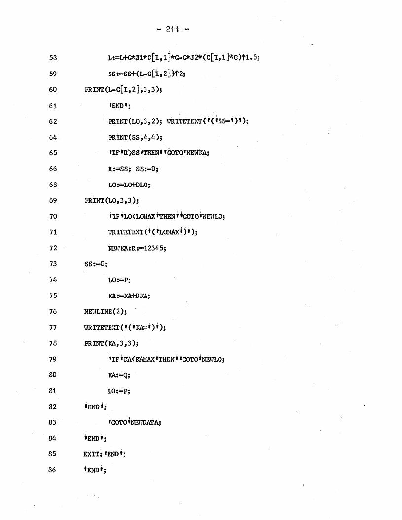
- 211; -

58 L:=L+G*Jl*c£lil>G-C3*J2*(C[l,l]*G)tl.5|

59 SS:=SS+(L-c[l,2])T2s

60 PRINT(L-C[X,2],3,3)5

61 »END*5

62 PRIlTr(LO,3,2)| tfRITETEXTO(f SS=t)f )s

64 PRINT(SS,4,4)j

65 tiFiR>SS^HEN**dCT0«lto]KA566 R:=SS| SSs=0$

68 LO:=LO+DLO$69 PRINT(LO,3,3>570 *if *LO<LOMAX *THEN *«GOTO*NEWLOs

71 W ITETEXT(KfL0MAX*)f )3

72 NEMKAtR:=12345|

73 SS:=0;74 LOs=P;75 KA:=KA+DKA;76 MEI7LINE(2)|

77 WRITETEXT<* (»I<A=*),)|78 PRINT(KA,3,3)5

79 *IF *I<A^KAMAX ♦THEN* *GOTO*NEWLO;

80 KA:=Q;81 LO:=P;82 »END*s83 * GOTO *NEI JD AT A j84 *END»;

85 EXIT:*END*S86 »END*5

- 212 -

APPENDIX 2The Justice Minimisation Method

( i 1 1In a recent discussion, Justice' ' made the interesting suggestion that one of the modified equations (of Fuoss-Hsia or of Pitts) might "be used to obtain the best-fit parameters, a, A 0 and as follows* The conductance equation is written in the form :

A = c< ( A 0 ~S( 0 c)2+ Ecln(oAc) + J^o4c *f* J2(o<c) )

.............i...(4.1)Initial values of /\ and (via an initial choice of K^) are then selected , and an ^experimental” value of J2 is obtained ( ( exp) ^ setting A equal to the experimental conductance /\^ :

J2(exp) = i ” ° ( A 0 - S(c^c)2 + Ecln( c<.c) + J^c))^ (okc)3/2

(4.2)

J is then calculated for a series of input a-values so as to find the minimum average deviation, A J , where :

fx~A J 2 V L (J2(exp) - J2> ( *3)

Ni.e. the summation is taken over the N data points A^jC^. A and o*\ are then varied, within acceptable limits, to improve the minimisation*

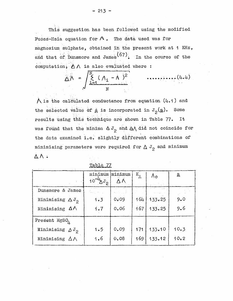
- 213 -

This suggestion has "been followed using the modified Fuoss-Hsia equation for A . The data used was for magnesium sulphate, obtained in the present v/ork at 1 KHz, and that of Bunsmore and JameS^"^* In the course of the computation^ A A is also evaluated where :

— ... .— ■— x

( /h - A )2 (^-h)1 ^

N

/\ is the calculated conductance from equation (h.l) and the selected value Of a is incorporated in JgCll)* Some results using this technique are shown in Table 77* It was found that the minima A J^ and /\/\ did not coincide for the data examined i.e. slightly different combinations of minimising parameters v/ere required for A an^ m nimumA A .

Table. 77

. _______;..;..

minimumi 0_4AJ2

minimumA A

ka Ao a

?Dunsmore & James •Minimising AJg 1*3 0*09 16U 1 3 3 .2 5 9.0Minimising A A 1.7 0.06 167 1 3 3 .2 5 9.6

Present MgSC^Minimising A 2 1.5 0 .0 9 171 1 3 5 .1 0 10.3Minimising A A 1.6 0.08 169 13 3 .1 2 10*2

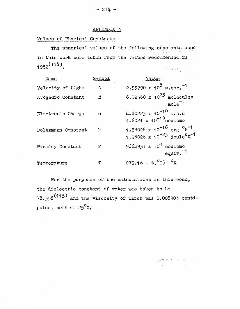
- 214 -

APPENDIX 3 Values of Physical Constants

The numerical values of the following constants used in this work were taken from the values recommended.in

Name __Velocity of Light CAvogadro Constant N

Electronic Charge e

Boltzmann Constant k

Faraday Constant

Temperature

F

T

Value ,■2.99790 x 109 m. sec. **6.02380 x 1023 molecules

-1mole4.80223 x I0*“i0 e.s.u 1.6021 x 10“1^coulomb1.38026 x 10~i6 erg °K ^1.38026 x 10~23 joule0K“19.64931 x 10^ coulomb

. -1 equiv.27 3 .1 6 + t(°C) K

For the purposes of the calculations in this work,the dielectric constant of water was taken to be

(115)78.358 and the viscosity of water was 0.008903 centi-poise, both at 25 C.

PART IV SECTION 3

REFERENCES

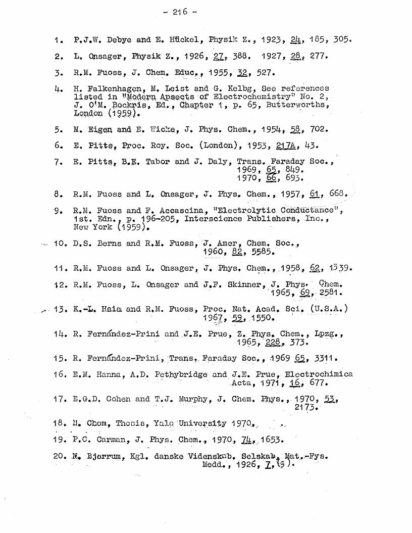
- 216 -

1, P.J.W. Debye and E. Hiickel, Physik Z., 1923, gjfc, 185, 305«2. L. Onsager, Physik z . , 1926, 22, 388. 1927, 26, 277.3, R.M. Fuoss, J. Chem. Educ., 1955, 2jLt 527.4. H. Falkenhagen, M. Leist and G. Kelbg, See references

listed in ’’Modern Apse.Qt.S of Electrochemistry” No. 2,J. 0*M. Bockris, Ed., Qh.apt.er 1, p. 6 5, But ter worths, London (i§5.9j*

3. M. Eigen and E. Wicke, J. Phys. Chem. , 1954, j>8 , 702.6. E. Pitta, Proe. Roy. Soc. (London), 1.953, 217A. 43.7. E. Pitts, B.E, Tabor and J. Daly, Trans. Faraday Soc. ,

1969, 65, 849.1970, bS, 693.

8. R.Ivl. Fuoss and L. Onsager, J. Phys. Chem., 1957, 61 . 66 8.9. R.M. Fuoss and F. Accascina, ’’Electrolytic Conductance”,

1st. Edn.. p. 196-205, Interscience Publishers, Inc.,New York (1959).

•— 10. D.S. Berns and R.M. Fuoss, J. Amer, Chem. Soc.,19 6 0, 8 2, 5585.

11. R.M. Fuoss and L. Onsager, J. Rhys. Chem. , 1958, 6 2 . 1339.

12. R.M. Fuoss, L. Onsager and J.F. Skinner, J. Phys* ' Qhem.1965 , ^ , 2581.

13. K.-L. Ilnia and R.M. Fuoss, Proc. Nat. Acad. Sci. (U.S.A.)1967 , £ 2 , 1550. ................

14. R. Fernandez-Prini and I.E. Prue, Z. Phys. Chem,, Lpzg,,1965. 228 . 373.

15* R. Fernandez-Prini, Trans.. Faraday Soc, , 1 9 6 9 6£ , 3311.

16. E.M. Hanna, A.D. Pethybridge and J.E. Prue, ElectrochimicaActa, 1971, 1 6 , 677.

17. E.G.D. Cohen and T.J. Murphy, J. Chem. Phys., 1970, 53 .2173.

18 . M. Chora, Thesis , Yale. U n iv e rs ity 1970....

19. P.C. Carman, J. Phys. Chem.,, 1970, 7 4 . 1653.

20. N* Bjorrum, Kgl. danske Videnskab. Selskab. Mat.-Fys.Medd. , 1926, I,\f )•

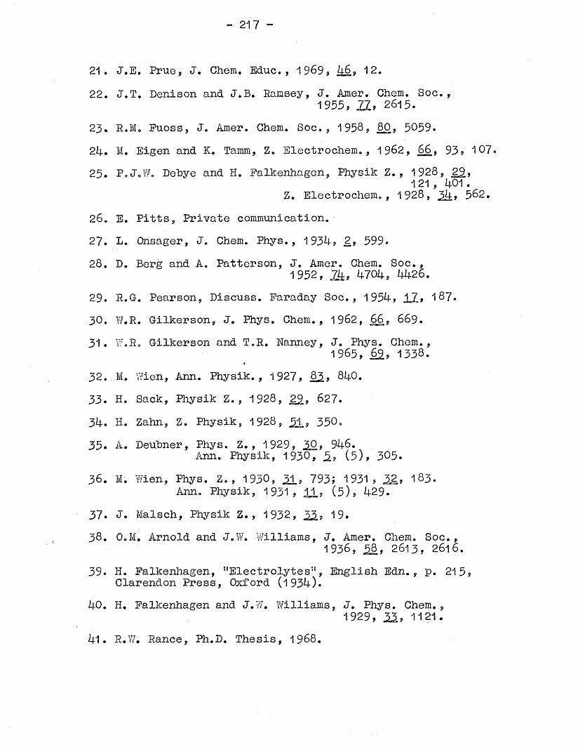
- 217 -

21. J.E. Prue, J. Chem, Educ., 1969, H , 12.22. J.T. Denison and J.B. Ramsey, J. Amer. Chem. Soc.,

1955, 12, 2615.23. R.M. Fuoss, J. Amer. Chem. Soc., 1958, 80, 5059.24. M. Eigen and K. Tamm, Z. Blectrochem., 1962, 6 6, 93, 107.25. PoJ.Wo Dehye and H. Falkenhagen, Physik Z. , 1928, 22,

1 21 , 401 .Z. Electrochem., 1928, 2k> 562.

26. E. Pitts, Private communication.27. L. Onsager, J. Chem. Phys., 1934, 2, 599.28. D. Berg and A. Patterson, J. Amer. Chem. Soc.,

1952, 24, 4704, 4426.29. R.G. Pearson, Discuss. Faraday Soc., 1954, 17. 187.30. W.R. Gilkerson, J. Phys. Chem., 1962, 6 6, 6 6 9.31. W.R. Gilkerson and T.R. Hanney, J. Phys. Chem.,

1965, 62, 1338.32.. M. Wien, Ann. Physik., 1927, 8 3. 840.33. H. Sack, Physik Z., 1928, 22? 627*34. H. Zahn, Z. Physik, 1928, 21,, 350.35. A. Deubner, Phys. Z., 1929, 20, 946.

Ann. Physik, 1930, 2, (5), 305.3 6. M. Wien, Phys. Z. , 1930, 21, 793; 1931, 22, 1 8 3.

Ann. Physik, 1931, 11? (5), 429.37. J. Malsch, Physik Z., 1932, 21? 19.3 8. O.M. Arnold and J.W. Williams, J. Amer. Chem. Soc.,

19 3 6, 21? 2 6 1 3, 2616.39. H. Falkenhagen, "Electrolytes”, English Edn., p. 215,

Clarendon Press, Oxford (1934).40. H. Falkenhagen and J.W. Williams, J. Phys. Chem.,

1929, 21? 1121.41. R.W. Ranee, Ph.D. Thesis, 1968.

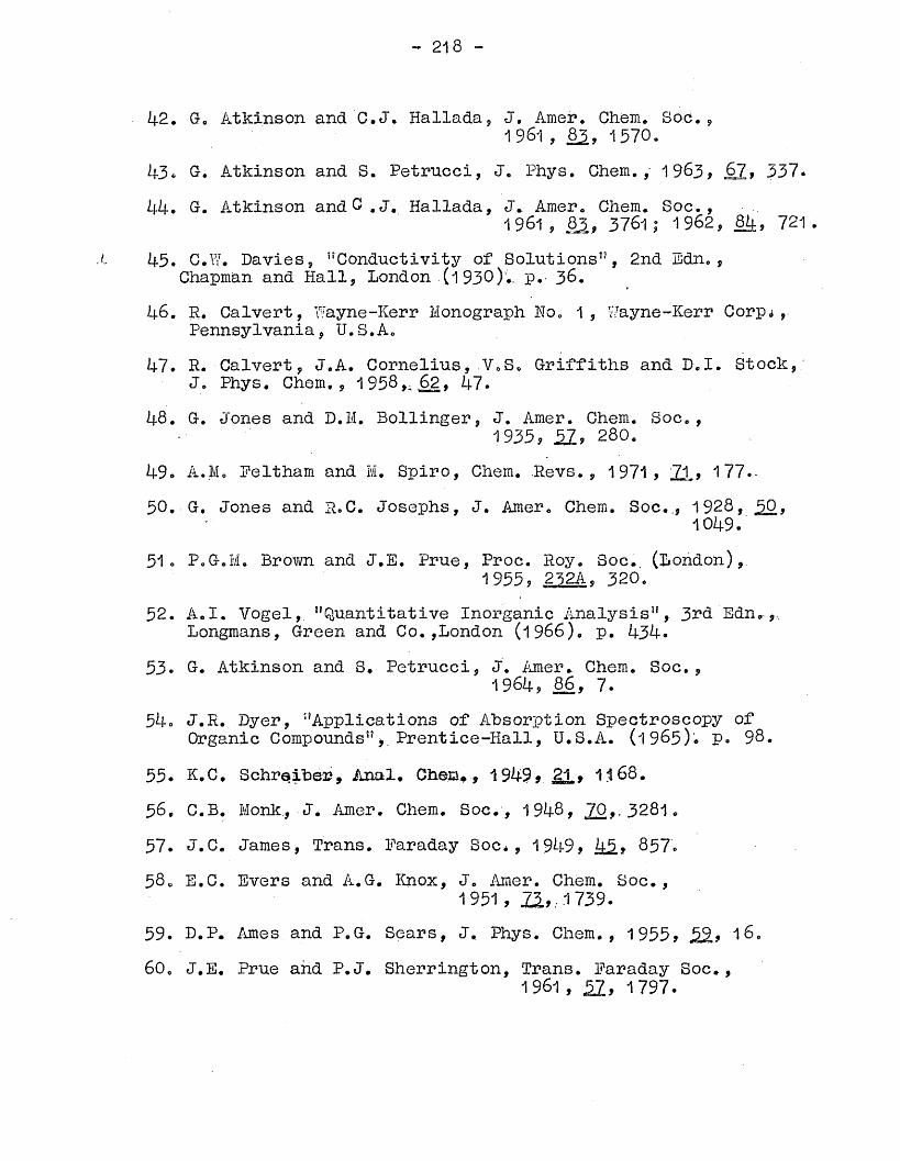
- 218 -

k2. G. Atkinson and C.J. Hallada, J. Amer. Chem. Soc.,1961,82,1570.

43. G. Atkinson and S. Petrucci, J. Phys. Chem., 1 9 6 3, 62, 337.44. G. Atkinson andC.J. Hallada, J. Amer. Chem. Soc.,

1961, 82, 3761,- 1962, 84, 721 .i 45. C.W. Davies, "Conductivity of Solutions", 2nd Edn.,

Chapman and Hall, London (1930)*- P.- 36.46. R. Calvert, Wayne-Kerr Monograph Ho. 1, Wayne-Kerr Corp«i ,

Pennsylvania, U.S.A.47. R. Calvert, J.A. Cornelius, V.S. Griffiths and D.I. Stock,:

J. Phys. Chem,, 1958,; 62, 47.48. G. Jones and D.M. Bollinger, J. Amer. Chem. Soc.,

1935, 21, 280.49. A.M. Feltham and M. Spiro, Chem. .Revs., 1971 , 71, 177.-50. G, Jones and R.C. Josephs, J. Amer. Chem. Soc., 1928, 50.

1049.51o P.G.M. Brown and J.E. Prue, Proc. Roy. Soc. (London),

1955, .232A, 320.52. A.I. Vogel, "Quantitative Inorganic Analysis", 3**d Edn.

Longmans, Green and Co.,London (1966). p. 434.53. U. Atkinson and S. Petrucci, J. Amer. Chem. Soc.,

1964, 86, 7.54. J.R.. Dyer, "Applications of Absorption Spectroscopy of

Organic Compounds" Prentice -Hall, U.S.A. (1 9 6 5). p. 98.55. K.C. Schreiber, Anal. Chem*, 1949. 21 . 1168.5 6. C.B. Monk., J. Amer. Chem. Soc. , 1948, 70., 3281.57. J.C. James, Trans. Faraday Soc*, 1949, 42? 8 5 7.58. E.C. Evers and A.G. Knox, J. Amer. Chem. Soc. ,

1951, 22,..1739.59. D.P. Ames and P.G. Sears, J. Phys. Chem., 1955, 22? 1 «60. J.E. Prue and P.J. Sherrington, Trans. Faraday Soc.,

1961 , 22? 1797.

j, 219

61; J.E. Prue, J'i Phys. Chem., 1963, 67, 1152.62. A. Deubner and Ri, Heise, Ann. Physik, Lpzg., 1951, 2, 213-63. "International Critical Tables", 1st Edn., Vol. Ill, p. 24,

Me Graw-Hill Book Co., Inc., New York (1926).64. J.E. Lind, J*J. Zv/olenk and R.M. Fuoss,

J. Amer. Chem. Soc., 1959, 81.? 1557.65. G. Jones and B.C. Bradshaw, J. Amer. Chem. Soc.,

1933, 22? 1780.66. H.C. Parker, J. Amer. Chem. Soc., 1923, 42? 1366, 2017.67. H.S. Dunsmore and J.C. James, J. Chem. Soc., 1951 , 2925*68. C.W. Davies, "Ion Association", 1st Edn., Butterworths,

London (1962). p. 12.69. A.S. Brown and T. Shedlovsky, J. Amer. Chem. Soc.,

1934, 2§? 1066.70. I.L. Jenkins and C.B. Monk, J. Amer. Chem. Soc.,

1950, 72, 2695.71. R.M. Fuoss and C.A. Kraus, J. Amer. Chem. Soc.,

1933, 22? 476.72. R.M. Fuoss, J. Amer. Chem. Soc., 1935, 22? 488.73. T. Shedlovsky, J. Franklin Inst., 1938, 225. 739.74. H.M. Daggett, J. Amer. Chem. Soc., 1951, 23, 4977*75. R. M. Fuoss and T. Shedlovsky, J. Amer. Chem. Soc.,

1949, 21, 1496. .76. M.l. Kilpatrick, J. Chem. Phys., 1940, 8, 306.77. W.G. Davies, R.J. Otter and J.E. Prue, Disc. Faraday Soc.,

1957, 24, 106,123.78. E.M. Hanna, A.D. Pethybridge and J.E. Prue, J. Phys. Chem.,

1971 , 22 ? 291.79. E.A. Guggenheim, Disc. Faraday Soc., 1957, 2 4, 6 4.80. J.E. Prue, "Ionic Equilibria", 1st Edn., Pergamon Press,

(1966). P. 33.81. M. Leist, Z. Physik. Chem., lpzg., 1955, 205. 1 6.

- 220 -

82. R.A. Mathe^on, J. Phys. Chem., 1968, J2, 3330.8 3. A. D’Aprano and R*M. Fuoss, J* Phys. Chem.,

1968,22,4710.84. 1.0. Mckenzie and R.M. Fuoss, J. Phys* Chem., 1969, 73.

. 1501.85. R.M* Fuoss, Rev* Pure and Appl. Chem., 1968, 1 8 , 125.8 6. R.M. Fuoss and K.-Li Hsia, J. Amer. Chem. Soc.,

1 9 6 8, 90, 3055.87. Y.-C* Chiu and R.M. Fuoss, J. Phys. Chem., 1968, 72.

. 4123.8 8. Ref. 8 5, P. 131.89. J.-C. Justice, Electrochimica Acta, 1971, 1 6 , 701.90. Ref. 9, P. 203.91. M.J.D. Powell, The Computer Journal, 1965, 2? 155, 303.92. A . DfAprano and R.M. Fuoss, J. Amer. Chem. Soc.,

1969, 21, 279.93. Hef. 54 P. 52.94. H.W. Jones and C.B, Monk, Trans. Faraday Soc., 1952, 48.

929.95. R.A. Robinson and R.H. Stokes, "Electrolyte Solutions",

2nd Edn., Butterworths, London (1959). p. 412.96. V.S.K. Pair and G.H. Rancollas, J. Chem. Soc., 1958, 3706.97. G.H. ITancollas, Disc. Faraday Soc., 1957, 2 4, 108.98. G. Atkainson and S. Petrucci, J. Phys. Chem.,

1966, 22, 3122.99. S. Petrucci, P. Hemmes, and M. Battistini, J. Amer. Soc.,

1967, 82, 5552.100. G. Atkinson and S. K. Kor,J. Phys. Chem., 1965, 6j}, 128.101* L.G. Jackopin and E Yeager, J. Phys. Chem., 1970, 22?

3766.102. P. Hemmes, F. Fittipaldi and S. Petrucci, Acustica,

1969, 21, 228.

- 221 -

103. 0. Atkinson and S. Petrucci, J. Phys. Chem., 1963, 6 7»337.

104. BiB. Ovv.cn and H. Zeldes, J. Chem., Phys,, 1950, 18, IO83.105. E.L. Carstensen, J. Acoust, Soc. Am., 1954, 26, 86 2.106. J.R* Smithson and T.A. Litovitz, J. Acoust. Soc. Am.,

1956, 28, 462.107. 0. Atkinson, S.K. Kor, and S. Petrucci,

Proc. Inst. Elect, Electron. Engineers, 1965, 13? 1355.108. F.E. Pox and T.M. Marion, J. Acoust. Soc. Am.,

1953, 2 5, 661.109. L.G. Jackopin and E. Yeager, J. Phys. Chem., 1966, 70.

313.110. R. Lovas, G. Macri and S. Petrucci, J. Amer. Chem. Soc.,

1970, 22, 6502.111. G. Macri and S. Petrucci, Inorg. Chem., 1970, 2, 1009.112. D.P. Evans and P. Gardam, J. Phys. Chem., 1969, 21? 198.113. J.-C. Justice, at a Discussion of the Electrochemical

Society (14-1 2-1 971 ).114. F.D. Rossini, EAT. Gucker, II.L. Johnston, L. Pauling,

and G.W. Vinal, J. Am. Chem. Soc., 1952, 24? 2699.115. B.B, Owen, R.C. Miller, C.E. Milner and II.L. Cogan,

J. Phys. Chem., 19 6 1, 6 3, 2065.