the efficiency of equity- linked compensation ... files/00-056_26efecae-5cf8-4b4a... · 3...

Copyright © 2000 Lisa K. Meulbroek

Working papers are in draft form. This working paper is distributed for purposes of comment and discussion only. Itmay not be reproduced without permission of the copyright holder. Copies of working papers are available from theauthor.

00-056

The Efficiency of Equity-Linked Compensation:Understanding the Full Costof Awarding Executive StockOptions

Lisa K. Meulbroek

Harvard Business SchoolSoldiers Field RdBoston, MA 02163

The author thanks Brian Hall, Josh Lerner, Mark Mitchell, André Perold, and Peter Tufano, aswell as seminar participants the Harvard Business School, University of Wisconsin, GeorgetownLaw School’s Conference on Highly-Paid Employees, and Tel Aviv University’s Accountingand Finance Conference, Lemma Senbet and Alex Triantis (the editors), as well as ananonymous referee for helpful comments. Andrew Kim provided excellent research assistance,and Harvard Business School’s Division of Research provided financial support for this project.E-mail: [email protected].

mailto:[email protected].

Abstract

The incentive-alignment benefits of equity-lined compensation are well-known, but relativelylittle attention has been devoted to identifying and measuring certain deadweight costs thatinevitably accompany such programs. To properly align incentives, the firm’s managers must beexposed to firm-specific risks, but this forced concentrated exposure prevents the manager fromoptimal portfolio diversification. Because undiversified managers are exposed to the firm’s totalrisk, but rewarded (through expected returns) for only the systematic portion of that risk,managers will value stock or option-based compensation at less than its market value. This paperderives a method to measure this deadweight cost, which empirically can be quite large:managers at the average NYSE firm who have their entire wealth invested in the firm value theiroptions at 70% of their market value, while undiversified managers at rapidly growing,entrepreneurially-based firms, such as Internet-based firms, value their option-basedcompensation at only 53% of its cost to the firm. These estimates prompt questions of whethercompensation plans in such firms are weighted too heavily towards incentive-alignment to becost effective.

2

I. Introduction

Finance theory has long made the case for the use of equity-linked compensation plans as an

effective means to align managers’ incentives with those of shareholders. In the last decade,

finance practice, particularly in the United States, has embraced this prescription, with stock-

options and restricted-stock plans forming a vastly increased proportion of senior management’s

total compensation. Although financial theory recognizes that the benefits from these plans are

inevitably tempered by certain deadweight costs to the firm, relatively little empirical work has

been devoted to identifying and measuring those costs. In essence, the exposure to firm-specific

risk that is essential for generating the right managerial incentives also imposes a cost on

managers by compelling them to hold less-than-fully-diversified investment portfolios. Every

firm faces this unavoidable tension between incentive alignment and portfolio diversification; the

optimal tradeoff between them will differ from firm to firm. This paper focuses on the costs

associated with this tradeoff, where the cost reflects the difference between the market value of

the instruments granted, and the value placed on those instruments by the managers who receive

them as substitutes for cash compensation.

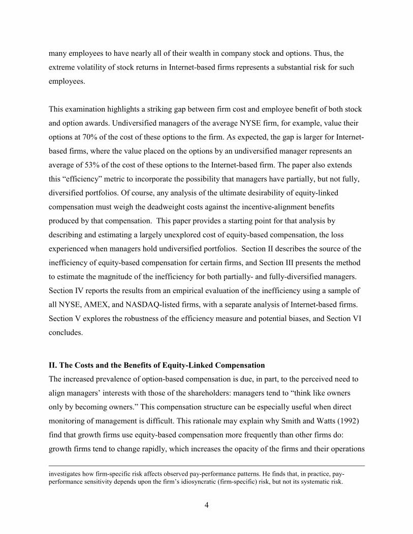
As managerial diversification declines, the “efficiency” of awarding equity-linked compensation

suffers. More precisely, the value of equity-linked compensation to undiversified managers may

be much less than the cost of providing this compensation to the firm. The undiversified manager

is exposed to the total volatility of the firm, whereas diversified investors bear (and are paid for)

only the systematic portion of the firm’s risk. The managers’ expected returns are therefore too

low to properly compensate them for the risks they face. Consequently, the value that

undiversified managers place on equity-based compensation is less than its market value.

Viewed in isolation from its incentive alignment benefits, this difference between the value of

equity-based compensation to undiversified managers, and the market-value of the equity-linked

security, represents a deadweight loss to the firm. That is, the firm could receive the full value of

equity-linked securities to a diversified investor by simply issuing such securities in the open

market. The deadweight loss, then, consists of non-negative difference between the higher value

of the securities to a diversified investor, and the lower value of the securities to the non-

3

diversified employee.1 This loss is greatest for high-volatility firms where managers have most

of their personal wealth tied up in the firm.

This paper offers a technique to measure the difference in value between the firm’s cost of

issuing equity, and the value that undiversified investors place on this form of compensation. The

paper departs from the previous finance and accounting literature on private valuation of

executive stock options by focusing on the costs explicitly incurred due to the loss of

diversification.2 The paper also advances our understanding of the cost of risk. Most principal-

agent models assume that all types of risk, whether systematic or non-systematic, are equally

costly to managers (agents). In contrast, this paper identifies non-systematic, firm-specific risk as

more costly to managers, because the expected market return fairly compensates managers for

bearing systematic risk, but does not compensate the managers for bearing non-systematic risk.

And indeed, while financial engineering has the potential to reduce the manager’s exposure to

systematic risk, managers must be exposed to this non-systematic, firm-specific risk to produce

the right incentives.

This paper then applies the suggested technique to measure the private value a manager places

on the firm’s stock, investigating the deadweight costs associated with stock- and option-based

compensation for a broad sample of firms. The paper also examines these costs for a set of firms

where the potential for which the costs are likely to be great, namely Internet-based firms. Such

firms tend to have relatively high levels of insider ownership, and typically much of the

employees’ pay comes from equity-linked compensation. Moreover, it is not uncommon for

1 I call the gap between managers’ private value and the firm’s cost a “deadweight cost” to distinguish it from themarket value of the firm’s compensation, which is the usual definition of “cost” in the executive compensationliterature.2 To be sure, a substantial literature investigates how features such as the probability of managerial departure (andsubsequent option forfeiture), the non-tradability of options, and early exercise patterns affect option value. See, forexample, Carpenter (1998) on how to adjust stock option value for the probability of forfeiture, Detemple andSundaresan (1999), Hall and Murphy (2000a), Hall and Murphy (2000b), Huddart (1994), Kulatilaka and Marcus(1994), and Lambert, Larcker and Verrecchia (1991) on non-tradability, early exercise, and employee risk aversion,and Johnson and Tian (2000) on various other characteristics of executive stock options, such as re-pricing and re-loading. The existing literature, however, has not specifically addressed how the deadweight costs associated withthe lack of diversification (the only feature that is inexorably bound to compensation designed to align incentives)affect managers’ private value of the option. Because the principal-agent models employed in the prior literaturehave only one risky asset, diversification (or lack thereof) does not enter into those models. Jin (2000), departingfrom the standard practice of treating both systematic and non-systematic risk as equally costly for managers,

4

many employees to have nearly all of their wealth in company stock and options. Thus, the

extreme volatility of stock returns in Internet-based firms represents a substantial risk for such

employees.

This examination highlights a striking gap between firm cost and employee benefit of both stock

and option awards. Undiversified managers of the average NYSE firm, for example, value their

options at 70% of the cost of these options to the firm. As expected, the gap is larger for Internet-

based firms, where the value placed on the options by an undiversified manager represents an

average of 53% of the cost of these options to the Internet-based firm. The paper also extends

this “efficiency” metric to incorporate the possibility that managers have partially, but not fully,

diversified portfolios. Of course, any analysis of the ultimate desirability of equity-linked

compensation must weigh the deadweight costs against the incentive-alignment benefits

produced by that compensation. This paper provides a starting point for that analysis by

describing and estimating a largely unexplored cost of equity-based compensation, the loss

experienced when managers hold undiversified portfolios. Section II describes the source of the

inefficiency of equity-based compensation for certain firms, and Section III presents the method

to estimate the magnitude of the inefficiency for both partially- and fully-diversified managers.

Section IV reports the results from an empirical evaluation of the inefficiency using a sample of

all NYSE, AMEX, and NASDAQ-listed firms, with a separate analysis of Internet-based firms.

Section V explores the robustness of the efficiency measure and potential biases, and Section VI

concludes.

II. The Costs and the Benefits of Equity-Linked Compensation

The increased prevalence of option-based compensation is due, in part, to the perceived need to

align managers’ interests with those of the shareholders: managers tend to “think like owners

only by becoming owners.” This compensation structure can be especially useful when direct

monitoring of management is difficult. This rationale may explain why Smith and Watts (1992)

find that growth firms use equity-based compensation more frequently than other firms do:

growth firms tend to change rapidly, which increases the opacity of the firms and their operations

investigates how firm-specific risk affects observed pay-performance patterns. He finds that, in practice, pay-performance sensitivity depends upon the firm’s idiosyncratic (firm-specific) risk, but not its systematic risk.

5

to outsiders.3 Yermack (1995) reinforces this observation, reporting that firms award stock

options more frequently when direct monitoring is difficult, that is, when accounting earnings

contain large amounts of “noise.”4

Many advocates of equity-based compensation focus almost exclusively on the benefits provided

by such compensation, devoting less attention to its costs. Indeed, if the only result of equity-

based compensation were incentive alignment, no natural “stopping-point” would exist:

managers’ compensation would be 100% equity-based. Yet, in practice, managers’ pay has

appeared to depend far less on firm performance than this naïve recommendation would suggest.

Jensen and Murphy (1990), for example, report that managers’ share of increases in firm value

averaged around three percent. In later work, Hall and Liebman (1998) find that by more

exhaustively incorporating the value of executive stock options into the calculations, this

sensitivity increases, but still remains relatively low.

What then prevents firms from increasing this pay-performance sensitivity? One answer is that

the current sensitivity is enough to spur managers to better performance. Murphy (1985) and

Core and Larcker (2000) provide some support for this hypothesis, with evidence presented by

Larcker (1983), DeFusco, Zorn and Johnson (1991), and McConaughy and Misha (1996)

somewhat more mixed. Another answer is that there are costs to such compensation, such as

encouraging managers to take too much risk. But theoretical and empirical work casts doubt on

whether options cause excessive managerial risk-taking, and even suggests that options might

provide managers with an incentive to decrease risk. See Carpenter (2000), Haugen and Senbet

(1981), Detemple and Sundaresan (1999), Cohen, Hall and Viceira (2000), and Rajgopal and

Shevlin (1999).

Another cost associated with equity-based compensation is the deadweight loss incurred when a

firm pays managers in a currency that they value less than its cost to the firm. The exposure to

3 Gaver and Gaver (1995)’s findings are consistent with those of Smith and Watts (1992).4 Incentive alignment is not the only perceived benefit of stock option plans. Dechow, Hutton and Sloan (1997)report that when Congress restricted the tax deductibility of executive compensation that is not incentive-based to$1million, most firms complied by replacing any cash compensation over the $1 million threshold with executivestock options. They also discuss a 1992 meeting FASB held with compensation consultants, who agreed that

6

firm-specific risk is both necessary to produce the right incentives and inevitably results in

managers losing some degree of diversification on their investment portfolios.5 Managers’

human capital investments in the firm,6 pension fund holdings skewed towards the company’s

stock, and deferred compensation plans7 all have the potential to increase managers’

idiosyncratic risk exposure substantially.

As a consequence, managers face an extraordinary level of risk with respect to their personal

portfolios, risk that outside investors who are able to hold diversified portfolios do not face.8 An

investor with her wealth invested solely in the average NYSE firm, for example, faces an annual

volatility of 45%, twice that of the 22% annual volatility faced by an investor who is all-equity

invested in a diversified market basket of stocks. Undiversified investors in volatile, Internet-

based firms face even higher risk, on average five times the risk borne by a diversified investor

(the volatility of Internet-based firms averages 117%, as shown in Table I)

Even more importantly, managers are not compensated for this additional risk with higher

expected returns. To adequately compensate the undiversified manager, the expected return of

the stock would need to be commensurate with its total volatility, and not only its systematic risk

component. But, the expected return is set by the firm’s incremental contribution to the volatility

of the market portfolio, not the total volatility, and is therefore too low to fully compensate the

manager for her risk exposure. As a consequence, the manager will value equity-linked

compensation at less than its market value, which represents the cost of the compensation to the

firm. 9 It is this “wedge” between the firm’s cost and the manager’s value that is the focus of this

accounting provisions affected the design of stock option plans. Long (1992) investigates whether taxes orincentives motivate a firm’s adoption of an executive stock option plan.5 Even a CEO’s cash compensation is subject to firm-specific risk: Lambert and Larcker (1988) find that 25% of thetime-series variation in a CEO's cash compensation is related to her firm's performance.6 Friend and Blume (1975) estimate that, on average, the human capital of individuals (including the value of anyprivately owned businesses) constitutes 52% to 87% of their total assets; some portion of that human capital will nodoubt be specific to the firm. See Degeorge, Jenter, Moel and Tufano (2000) for a discussion of how employee’shuman capital affects her decision to buy her employer’s stock.7 Deferred compensation is a general liability of the firm, again exposing the manager to firm-specific risk.8 Managers may be able to reduce some of their risk through targeted financial instruments (see footnote 11). Toaccount for the possibility that managers can reduce their exposure the analysis below specifically derives anefficiency metric for both a fully- and a partially-diversified investor.9 Firms do buy back stock in the open market so that they can issue equity to managers without “diluting” the firm’sshareholders. So, the market value of equity-based compensation seems a good estimate of the firm’s cost, whetherone considers it an opportunity cost (what the market would pay for the instrument), or a real one.

7

paper. 10 The wedge compels a firm with undiversified managers or employees to choose

between issuing options to the market, and receiving their full value from outside investors, or

granting the options to insiders, who will not value them as highly. Indeed, if one were to ignore

the incentive-alignment benefits of equity-based compensation, the firm and its employees would

be better off if the firm were to sell the options to outsiders, and then give the cash proceeds of

such sales to its employees.

Does the forced exposure to the firm’s total risk impose a substantial cost on managers? On the

one hand, firms do continue to issue options to their managers. On the other hand, managers

appear to be taking any steps possible to reduce their risk exposures. Managers have, for

example, been using swaps or zero-cost collars to reduce their risk.11 And, it is the managers of

especially risky firms, such as Internet-based firms, who sell their holdings at a higher rate than

managers of other firms. Meulbroek (2000a) reports that 93% of all corporate insider

transactions in Internet-based firms are sales, versus 63% in non-Internet-based firms. These

sales occur despite the hefty taxes that managers typically face upon selling their holdings,

suggesting that managers put a high value on decreasing their risk by selling shares.

The importance of risk to managers is reinforced by the finding that managers frequently

exercise their options prior to expiration, even on non-dividend paying stocks. Ofek and

Yermack (2000) find that managers sell almost all shares acquired through option exercise,

10 Several papers provide good discussions of why managers value equity-linked compensation at less than thefirm’s cost of awarding that compensation. See, for example, Abowd and Kaplan (1999), Carpenter (1998),Lambert, Larcker and Verrecchia (1991), Murphy (1998) or Smith and Zimmerman (1976).11 The manager obtains the swap or zero-cost collar over-the-counter, typically from an investment bank. Suchinstruments are economically similar to selling the stock, but have different tax implications, and seem not to attractthe same degree of public scrutiny as straight stock sales do. Bettis, Bizjak and Lemmon (2000) describe thesecontracts, and reports that the number of such transactions reported to the SEC has, so far, been relatively small.Bettis, Bizjak and Lemmon (2000) also find, however, that the SEC’s reporting requirements for these transactionshave only recently been clarified, so that the true incidence of zero-cost collars is perhaps higher than the historicalstatistics would suggest. Another way that managers might seek to limit their exposure to market risk is to shortS&P 500 futures to offset the systematic risk inherent in their positions in company stock. While a theoreticalpossibility, in practice, few managers appear to engage in such transactions, perhaps because of the liquidity riskinduced by this strategy. That is, managers would have to mark-to-market their S&P 500 positions daily, and postadditional margin in case of a market increase, but they would not be able to use their holdings in company stock oroptions to meet the margin call. Managers can also reduce risk through equity swaps (see Bolster, Chance and Rich(1986)), but changes in the tax code have made such swaps considerably less attractive. Boczar (1998) describesseveral (economically-equivalent) methods for an executive to manage risk, and the tax implications of suchmethods. See also Schizer (2000) on managerial hedging of stock option positions. Hedging of options can bedifficult for managers as many firms prevent executive stock options from being pledged as collateral.

8

which usually occurs as soon as the options vest. Huddart and Lang (1996) report that early

option exercise is more likely at riskier firms. These managerial sales have not gone unnoticed

in the financial press: Directors and Boards notes that “despite the massive issuance of stock

options, ownership levels of managers have not increased. Although touted as programs that

make managers think like owners, stock option programs appear more like short-term bonuses,

given the unwillingness of executives to retain their shares.”12

Of course, a desire to gain at least some degree of diversification in order to reduce risk is not the

only reason managers sell stock or exercise options. That risk reduction is an important motive,

however, is supported by Meulbroek (2000a)’s finding that the market does not react negatively

to managerial sales from Internet-based firms, differing significantly from the reaction to

managerial sales in non-Internet-based firms. These results suggest that managerial sales in a set

of risky firms do not appear to be motivated by managers’ inside information, and that the

market understands the great incentive that managers in such firms have to diversify.13

Consistent with Meulbroek (2000a)’s results on executive stock sales, Carpenter and Remmers

(2000) find that executive stock option exercises tend to take place for non-informational

reasons. These findings suggest that the wedge between the firm’s cost and the managers’ private

value of equity-linked compensation can be large. The next section more directly investigates the

magnitude of this wedge by developing a technique to estimate the undiversified investor’s

private value of the stock

III. Adjusting the Value of Equity-Linked Compensation for the Loss of Diversification

The total cost imposed on the manager by her compelled holding of equity-based compensation

has two components. The first is the cost associated solely with the loss in diversification. The

second is the cost arising from the specific pattern of risk exposure created by the financial

instrument the manager is required to hold (e.g. an option produces a certain dynamic exposure

to risk over time, and that pattern may not represent the manager’s preferred risk exposure, either

in level or timing). Financial engineering can reduce or eliminate the second component of

12 Directors and Boards, “The New Physics of Stock Options,” Winter, 1999.13 Although publicly-traded Internet-based firms tend to be larger, on average, than other publicly-traded firms, andstock price responses in larger firms tend to be less informative than managerial sales at smaller firms, Meulbroek

9

cost,14 but the first component, the cost due to lost diversification, cannot be eliminated without

destroying incentive alignment. That is, the cost due to lost diversification is the only structural

cost associated with incentive-based compensation, and is therefore the focus of this paper.

To estimate this loss-of-diversification cost, we calculate the expected return a manager would

require in order to be indifferent between holding a portfolio consisting only of the firm’s stock,

and holding an efficiently-diversified portfolio levered to a volatility level that equals that of the

firm’s stock. This method, which we call the Sharpe ratio approach, produces a lower-bound

estimate of the actual cost from the manager’s concentrated exposure because it does not account

for that manager’s individual preferences regarding the level or pattern of risk exposure she

faces. A manager’s utility function will determine the magnitude of this individual preference-

based cost, which can be measured via a “certainty-equivalent” approach if the manager’s utility

function were known. Prior literature has focused on estimating the individual-specific

component of cost, while implicitly assuming that there is no cost due to the loss in

diversification.15 The strength of our Sharpe ratio technique is that it isolates the one type of risk

that is essential to properly aligning incentives, and this firm-specific risk imposes a common

cost on all managers.16

Note that even the ability of managers to choose employers, and by extension, the type of

compensation package they receive, cannot reduce the deadweight costs associated with lost

(2000a) reports that these results are robust to firm size: even managerial sales at small Internet-based firms are notinterpreted by the market as information based.14 Options indexed to the market are one way to eliminate systematic risk via financial engineering – see Johnsonand Tian (2000), Meulbroek (2000b), Rappaport (1999) and Schizer (2001).15 For examples of this individual utility-based technique, see Hall and Murphy (2000a), Hall and Murphy (2000b),Huddart (1994), or Lambert, Larcker and Verrecchia (1991). If one wanted to explicitly incorporate costs of lostdiversification, the models used in these papers would have to be modified to incorporate more than one risky asset,along the lines of Jin (2000). Even then, using a specific functional form of a manager’s utility function to calculatea certainty-equivalent value conflates the effect of managerial preferences about the functional form of thecompensation plan with the effect due to lost diversification. For example, a manager holding a stock perfectlycorrelated with the market will effectively be fully-diversified. The Sharpe ratio method used in this paper tells usthat the efficiency of equity-based compensation is 100%, that is, the manager will value that stock at its full marketvalue. Yet, the utility-function approach tells us that the manager values this stock at less than its market value,simply because the risk exposure created by holding that stock is unlikely to be the optimal risk exposure for thatparticular manager.16 To measure the full cost to managers imposed by any given compensation system, the Sharpe ratio methodpresented here could be combined with the certainty-equivalent method used in prior research. Specifically, the lack-of-diversification cost estimated via the Sharpe ratio method would be used as an input to a utility-based approach.

10

diversification. Such self-selection may serve to reduce the loss due to individual preferences,

but any compensation plan that exposes managers to firm-specific risk will result in lost

diversification no matter how closely the package otherwise fits individual preferences. In this

sense, self-selection plays a role similar to that of financial engineering.

A. Derivation of an Efficiency Metric for Stock- and Option-based Compensation for the

Completely Undiversified Investor

We begin with the assumption that CAPM holds instantaneously in a continuous-time model, an

assumption consistent with the underlying assumptions of the Black-Scholes option-pricing

model, which we use later to value the executive options.17 This assumption is not critical in the

sense that the same method presented here could be adapted to incorporate any asset-pricing

model (of course, the numerical estimates will change, but the technique will not). These

assumptions produce mean-variance behavior. Interpreted in the context of this paper, mean-

variance behavior implies that even people with high risk tolerances, such as entrepreneurs,

prefer the higher expected return produced by a leveraged fully-diversified portfolio to the lower

expected-return from an equally risky single-stock portfolio.

In the Black-Scholes model, and in continuous-time portfolio theory, the security market line

relation is expressed in “instantaneous” expected-rates-of-return (i.e. exponential, continuous-

compounding):

( )j f j m fr r r rβ= + − (1)

where ( )1ffRre ≡ + where fR represents the riskless arithmetic return, and fr is

therefore its continuously-compounded equivalent.

≡er j (1 + yearly expected rate-of-return of security j under CAPM pricing)

17 Unlike the original single-period discrete-time version of the CAPM, the continuous-time version of the CAPMand its implied mean-variance optimizing behavior is consistent with limited-liability, lognormally-distributed assetprices, and concave expected utility functions. See Merton (1992) on the CAPM in continuous time. See also Blackand Scholes (1973). Adopting a continuous-time approach, combined with log-normally distributed security returnsyields mean-variance behavior without imposing the strict assumptions limiting the utility function to quadraticutility and normally distributed prices, as required by the discrete time model.

11

≡ujre (1 + yearly expected rate of return on security j required by an

undiversified mean-variance optimizing investor to make that investor indifferentbetween holding stock j, and holding a market portfolio with a volatility equal tothat of stock j)

( ) =− fm rr the market’s risk premium (continuously-compounded)

=mr the expected market return (continuously-compounded)

=mσ the market’s volatility

=jβ firm j’s beta from CAPM

=jσ firm j’s volatility

Define jujj rrs −≡ , the instantaneous spread between the expected return required by anundiversified investor relative to the CAPM-based expected return. This spreadrepresents the compensation an undiversified investor must receive in order to beindifferent between holding only stock j in her portfolio, and holding the marketportfolio.

i. Calculation of ujr and jr , the required rates of return under the CAPM by undiversified and

diversified investors.

This section presents calculations designed to address the question: what expected return would

an undiversified manager require to be indifferent between holding stock j in a single-stock

portfolio, and holding a market portfolio levered to firm j’s volatility? In other words, at each

point in time we examine the actual volatility level associated with the manager’s forced

concentrated holdings, and ask what expected return on stock j would make that manager

indifferent between stock j and the best portfolio possible.

If an undiversified investor had the market portfolio as an alternative investment opportunity,

and were a mean-variance efficient investor, she would require a risk-return ratio as good as the

market’s risk-return ratio in order to be indifferent between holding the market portfolio and a

portfolio composed exclusively of stock j. To calculate the excess return commensurate with

12

stock j’s risk-level, ujr , using the market’s risk-return ratio as a benchmark, we use the Sharpe

ratio:

( ) u

m f j f juj f m f

m j m

r r r rr r r r

σσ σ σ− −

= ⇒ = + −

(2)

And knowing ujr and jr yields js )( j

ujj rrs −≡ .

( ) ( )( )fmjmm

jfmj

m

jj rrrrs −−

=−

−

= ρ

σσ

βσσ

1 (3)

where jmρ is the correlation coefficient between firm j’s returns and the market returns. Figure I

displays this return premium graphically.

[insert figure I about here]

ii. Using js to calculate the value of stock j to an undiversified investor

Let ( ) ≡tV j value of stock j at time t (the market price).

≡T date at which the undiversified investor is free to sell the stock.

( ) ≡tV uj ( )( ), , , ,j j jG V t d sτ which is the private value placed on the stock of j by

investor forced to hold the stock j position undiversified until date T, where.tT −≡τ

In the analysis below, we assume for analytical simplicity that the firm does not pay dividends

during Tt ≤ , the duration of the sale restrictions. The zero-dividend assumption seems

reasonable for Internet-based firms, and young entrepreneurial firms more generally.

13

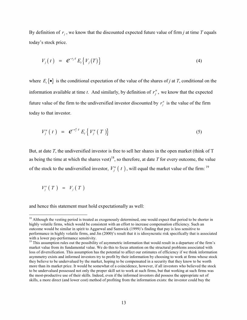
By definition of jr , we know that the discounted expected future value of firm j at time T equals

today’s stock price.

( ) ( ){ }jrj t jV t E V Te τ−= (4)

where { }tE • is the conditional expectation of the value of the shares of j at T, conditional on the

information available at time t. And similarly, by definition of ,ujr we know that the expected

future value of the firm to the undiversified investor discounted by ujr is the value of the firm

today to that investor.

( ) ( ){ }ujru u

j t jV t E V Te τ−= (5)

But, at date T, the undiversified investor is free to sell her shares in the open market (think of T

as being the time at which the shares vest)18, so therefore, at date T for every outcome, the value

of the stock to the undiversified investor, ( )ujV t , will equal the market value of the firm: 19

( ) ( )uj jV T V T=

and hence this statement must hold expectationally as well:

18 Although the vesting period is treated as exogenously determined, one would expect that period to be shorter inhighly volatile firms, which would be consistent with an effort to increase compensation efficiency. Such anoutcome would be similar in spirit to Aggarwal and Samwick (1999)’s finding that pay is less sensitive toperformance in highly volatile firms, and Jin (2000)’s result that it is idiosyncratic risk specifically that is associatedwith a lower pay-performance sensitivity.19 This assumption rules out the possibility of asymmetric information that would result in a departure of the firm’smarket value from its fundamental value. We do this to focus attention on the structural problems associated withloss of diversification. This assumption has the potential to affect our estimates of efficiency if we think informationasymmetry exists and informed investors try to profit by their information by choosing to work at firms whose stockthey believe to be undervalued by the market, hoping to be compensated in a security that they know to be worthmore than its market price. It would be somewhat of a coincidence, however, if all investors who believed the stockto be undervalued possessed not only the proper skill set to work at such firms, but that working at such firms wasthe most-productive use of their skills. Indeed, even if the informed investors did possess the appropriate set ofskills, a more direct (and lower cost) method of profiting from the information exists: the investor could buy the

14

( ){ } ( ){ }ut j t jE V T E V T= (6)

Substituting (6) into (4) and (5), we have

( ) ( ){ } ( ) ( )u uj j j ju

j t j j jr r r sV t E V T V t V te e e eτ τ τ τ− − −= = ⋅ ⋅ = (7)

The manager’s private value of the stock today is its market value today, discounted by the

incremental amount required to compensate the manager for the firm’s total risk. Figure II

displays this process graphically.

⇒ ( )( )

uj

j

jsV tEfficiency of Stock Compensation

V te τε −

≡ = = (8)

The “efficiency” of stock compensation to an undiversified investor, ε , is the ratio of the stock’s

value to an undiversified employee relative to the cost of that compensation to the firm. This

efficiency calculation does not assume or require that cash flows follow any particular pattern,

nor does it depend upon any specific valuation model.

[insert Figure II about here]

Equation 8 suggests that the longer a manager is constrained to hold an undiversified portfolio,

the less it is worth to her. It also reveals that efficiency increases with the stock’s correlation to

the market: the higher the correlation – or the stock’s beta – the closer the stock’s expected

return gets to the market’s expected return, which lowers js , the undiversified manager’s

required expected return premium. In the limit, a manager holding a single-stock portfolio which

happens to be perfectly correlated with the market will essentially be fully-diversified, and will

not require any additional return premium. Following equation 8, a three-year vesting period and

a 1% required expected return premium yields an efficiency of 97%, a 10% expected return

stock, and not seek employment. Finally, structuring a compensation system around the assumption (or hope) thatmanagers know the firm to be undervalued hardly seems a wise strategy.

15

premium decreases efficiency to 74%, and a 20% required expected return premium translates

into a 54% efficiency level. Loss of diversification has the potential to significantly affect the

manager’s private value of the firm’s stock.

Equation 8 also provides some support for our earlier speculation that start-up companies in risky

industries produce the greatest gap between the cost of equity-linked compensation and the value

of such compensation to undiversified insiders. Start-up firms are likely to meet the conditions

because they are often highly volatile, yet the volatility may, at first, be mostly a function of

firm-specific factors (e.g.. is the new product a success, can the firm get the necessary funding

for its projects, do suppliers provide the expected raw materials in a timely fashion), resulting in

a low β . Over time, as the new firm becomes better-established and overcomes the many

obstacles facing start-ups (logistical or otherwise), market risks may represent a larger proportion

of the firm’s total risk profile, so that β will increase even if σ remains unchanged. Today’s

market conditions create the potential for very low efficiency levels. That is, the confluence of

rapidly-changing technology, the emergence of many start-up firms to capitalize on this

technological change, coupled with a tendency for such firms to compensate management largely

through equity-linked compensation all play a role in reducing efficiency levels.

iii. Calculating the efficiency of option-based compensation: a two-stage approach

The derivation of the discount for lack-of-diversification on an option parallels that of the lack-

of-diversification for the stock, presented above, but is more complex because both the expected

return and the standard deviation of the option change at every point in time.20 As in the

discussion of the stock discount, we assume that the employee will be indifferent between

concentrated-versus-efficiently-diversified exposures if he or she is presented with the same

(instantaneous) Sharpe ratio in either case, which again produces a lower-bound on the

undiversified investor’s discount. This lower-bound results from the willingness of some

employees to give up an additional amount in expected return terms to change their total level of

risk or to pursue a dynamic risk strategy that differs from that of an option.

20 I thank Robert C. Merton for his assistance with this derivation.

16

We refer to the instantaneous expected return on the employee’s option as jor , where j is the

subscript representing the firm, and o represents “option”. As shown in Merton (1992, p.377,

(11.62)), the instantaneous expected return on the employee’s option is given by

2 212 j j VV j j v

jo

V f r V f fr

f

τσ + − = (9)

where ( ),f V τ is the Black-Scholes value of the option and subscripts on f denote partial

derivatives with respect to the share price V and time until expiration, τ .

Similarly, from Merton (1992, p. 377, (11.63)), we have the instantaneous standard deviation of

the return on the option, joσ , can be written as:

j j Vjo

V ff

σσ = (10)

It follows from (10) that the instantaneous expected excess return, jo fr r− , can be expressed as:

2 212 j j VV j j V f

jo f

V f r V f f r fr r

f

τσ + − − − = (11)

and taking the ratio of (11) to (10), we have that the instantaneous Sharpe ratio of the option

return is given by:

2 212 j j VV j j V f

jo f

jo j j V

V f r V f f r fr rV f

τσ

σ σ

+ − − − = (12)

17

Following the stock efficiency derivation, if we now require that the option be priced so that at

every point in time it has a Sharpe ratio equal to the Shape ratio of the market portfolio, we have

from (12):

2 212

m fj j V j j VV j j V f

m

r rV f V f r V f f r fτσ σ

σ−

= + − −

(13)

By rearranging terms, f must satisfy the partial differential equation:

( )2 2102

jj j VV j m f j V f

m

V f r r r V f r f fτ

σσ

σ

= + − − − −

(14)

Noting that ( )j jm j mβ ρ σ σ= and substituting for jr from (1) into (14):

( ) ( )2 2

from equation (3)

10 12

jj j VV f jm m f j V f

m

js

V f r r r V f r f fτ

σσ ρ

σ≡

= + − − − − −

(15)

where uj j js r r≡ − , the return premium that an undiversified investor in the stock would require

to make her indifferent between holding the stock and holding the market portfolio levered to the

volatility level of the stock. From (15) and the definition of js :

2 2102 j j j jVV Vf fV f r s V f r f fτσ = + − − − (16)

By inspection, this equation is the partial differential equation for the Black-Scholes option-

pricing formula on a stock which pays a proportional dividend at rate js (see Merton (1992, p.

295, (8.44)). The well-known solution to this partial differential equation is the Black-Scholes

formula for a proportional dividend on stock:

18

( ) ( )j frsj j j jV e N d X e N df ττ σ τ−− − −= (17)

where

( ) 21ln2j f j j

jj

V X r sd

σ τ

σ τ

+ − + =

Substituting (7), ( ) ( ) ( )ln ln lnj js su uj j j j j jV V e V V e V sτ τ τ− −= ⇒ = = − into equation (17),

we find that the pricing on an option that at every point in time provides an instantaneous

Sharpe-ratio equal to the instantaneous Sharpe ratio on the market portfolio is exactly the Black-

Scholes formula on a non-dividend paying stock where we replace the market price of the stock

jV by its discounted value, ujV ,

( ) ( )uj

frj j jf V N d X e N dτ σ τ−= − − (18)

( ) 21ln2

uj f j

jj

V X rd

σ τ

σ τ

+ + =

which is the Black-Scholes formula with ujV as the stock price. Therefore, the pricing on an

option that at every point in time provides an instantaneous Sharpe-ratio equal to the

instantaneous Sharpe ratio on the market portfolio is exactly the Black-Scholes formula on a

non-dividend paying stock where we replace the market price of the stock jV by its discounted

private value, ujV , as indicated below, where F represents the efficiency of the option.

( , , , , )( , , , , )

uj j f j

j j f j

f V T t r X VEfficiency of Option Compensation

f V T t r X Vσσ

− =Φ ≡ =

− =(19)

19

where the exercise price (X) is jV , the amount a manager would actually have to pay to exercise

the option, and the denominator is the market value of the option. Note that as most executive

stock options are issued at-the-money, for consistency we adopt the same convention.

iv. Stock efficiency versus option efficiency

The efficiency of the option is less than the efficiency of the underlying stock. To see this, note

that by the homogeneity property (Merton (1992), theorem 8.5) and the property that a lower

exercise price leads to a higher option value, we have21

( , ) ( , ) ( , ) ( , )u s s s sj j j jF V X F e V X F e V e X e F V Xτ τ τ τ− − − −= < =

And dividing by ( , )jF V X reveals that the option efficiency, F must always be less than the

efficiency, ε .

( , ) ( , )( , ) ( , )

u sj j s

j j

F V X e F V Xe

F V X F V X

ττ ε

−−Φ = < = =

The dynamics of option efficiency are similar to those for stock efficiency. As the expected rate

of return premium increases, option efficiency decreases, and as vesting periods increase, option

efficiency decreases. Changes in the required expected rate of return premium have a larger

effect on the option efficiency than do changes in the vesting period. And, as the time until

option maturity increases, efficiency increases, but only slightly.

B. An Efficiency Metric for Stock- and Option-based Compensation for the Partially-Diversified

Investor

The efficiency measures outlined above assume that the manager is compelled to hold all of her

wealth in equity or options of the firm and is therefore completely undiversified. While this

assumption may be a good approximation for managers in Internet start-up firms, managers in

more mature firms may have investment portfolios that are better diversified. If the manager is

able to at least partially diversify her holdings, the efficiency of equity-based compensation will

rise, but by how much? Under partial diversification, the volatility faced by the manager will be

a mix of the firm’s volatility and the volatility of the manager’s other holdings, and, as a

21 I thank Alex Triantis for pointing this out.

20

consequence, the premium required by the manager, js , will decrease. If we assume that the

manager achieves this partial diversification by investing some of her holdings in the market

portfolio (scaled by the riskless asset) we can again derive the value of equity-linked

compensation to this partially diversified manager (Appendix A contains this derivation). For

this partially-diversified investor with weight w invested in stock j and (1-w) in the market

portfolio, where σp equals the standard deviation of the combined market plus stock j portfolio,

the efficiency is:

( )( )

( ) ( ) ( )*

* ** 1Stock Efficiency , where 1j p m

j j j m fj m

j jr rV te r r r r

V t wτ σ σ

βσε − − −

= = = − = + − −

The option efficiency calculation parallels that for the case of the completely undiversified

investor.

Figures III and IV demonstrate graphically how partial diversification affects stock and option

efficiency respectively, corresponding to a hypothetical firm with the same mean and volatility

of the average firm (the equally-weighted average beta for all NYSE, NASDAQ and AMEX

firms is 0.77, with volatility of 65%). We can see that the ability to partially diversify helps, but

perhaps not as much as one might expect. For example, the ability to diversify by holding 50%

of one’s wealth in the market portfolio increases option efficiency to 63% (from the completely-

undiversified baseline of 54%)

[put figures III and IV about here]

IV. Illustrating Use of the Efficiency Metric Using Firm-Specific Data for NYSE, AMEX,

NASDAQ, and Internet-Based Firms

To better understand how economically significant the loss in efficiency for equity-based

compensation might be, this section applies the efficiency metrics derived above to a broad

sample of firms. Specifically, we calculate stock and option efficiency metrics for all NYSE,

21

AMEX, and NASDAQ firms listed as of December 31, 1998 examining separately the results for

a sample of Internet-based firms defined by the Hambrecht & Quist (H&Q) Internet Index.22

The efficiency metrics require estimates of β and σ for each firm as inputs. To estimate a firm’s

β, we use the market model, incorporating the last 150 trading days of returns data prior to

December 31, 1998, and using CRSP’s value-weighted market composite index. We use these

same 150 trading days of returns data to estimate each individual firm’s σ. The estimate of the

market’s volatility, σm uses the returns of CRSP’s value-weighted market composite index over

this same time period. We assume a risk-premium of 7.5% (7.2% continuously-compounded),

the historical average amount by which the value-weighted market index exceeds the long-term

government bond rate (monthly data begins in 1926).

Table II displays the summary statistics of the stock efficiency metric, ε*, applied to each

individual firm in the sample, for varying levels of managerial diversification and stock

restriction periods. Panel A of Table II shows these summary statistics for all Internet-based

firms, Panel B NYSE firms, Panel C AMEX firms, Panel D NASDAQ firms, and Panel E all

firms. Managers of NYSE firms have, on average, much higher stock efficiency levels than

managers of Internet-based firms or NASDAQ firms, at all levels of portfolio diversification. A

completely undiversified manager in an NYSE firm experiences a mean 77% stock efficiency

level (for a three-year required holding period on the stock), which drops to 66% for the longer

five-year vesting period. One would suspect that managers of NYSE firms are likely to be better

diversified than managers of Internet-based firms. If a manager of an NYSE firm had only 25%

of her total wealth invested in the firm, that manager would, on average, value stock

compensation at 91% of its cost to the firm for a three-year vesting period, and 85% for a five-

year vesting period.

The higher volatility of NASDAQ and Internet-based firms results in efficiency levels that are

substantially lower than those associated with NYSE firms. A completely undiversified manager

22 The H&Q Internet Index comprises a sub-sample of Internet-based firms, and is not confined to H&Q clients. TheInternet Index is widely-cited and viewed as a reliable reflection of Internet-based activity. Appendix B lists thesefirms, grouped by function.

22

with all of her wealth invested in an Internet-based firm values stock compensation at 55% of its

cost to the firm, for the three-year vesting period, a number that decreases to 38% if the vesting

period lasts five years. The stock efficiency ratings for NASDAQ firms are similar to the

Internet-based firms, but somewhat higher. Partial diversification helps increase efficiency, but

its absolute level remains low. The mean stock efficiency for an Internet-based manager with

50% of his wealth invested in the firm is 60% for the three-year vesting period, only five

percentage points higher than the manager with 100% of her wealth invested in the firm. If the

vesting period increases to five years, the mean stock efficiency decreases to 45% for the

manager able to hold 50% of her wealth outside the firm.

Table III, with Panels A through E shares a similar structure to Table II, but provides summary

statistics for option efficiency levels for varying levels of diversification, vesting periods, and

option maturity levels. We approximate the value of an executive stock option using the Black-

Scholes option pricing formula. Strictly speaking, the Black-Scholes formula provides the

approximate value, rather than the exact value, of an executive stock option.23 For simplicity and

clarity, however, we present the results using the Black-Scholes value, recognizing that the

estimates are only approximate.

The completely undiversified manager values executive stock options at 53% of their cost to the

mean Internet-based firm, assuming a three-year vesting period, and ten-year options. This

number increases to 55% if the manager is able to keep 25% of her wealth outside the firm, or

59% if the manager is able to keep 50% of her wealth outside the firm. See Appendix C for a

more detailed display of stock- and option-efficiency levels for individual Internet-based firms.

As with the stock efficiency numbers, the mean option efficiencies for NASDAQ firms are very

similar to those of Internet-based firms. Finally, the mean gap between the manager’s private

value of executive stock options and the cost of those options to the firm is lower for NYSE

firms, but it is not insignificant. The mean efficiency associated with a three-year vesting period

23 The formula is an approximation because executive stock options have some of the features of American options(i.e. exercisable at any time after the options vest, whereas the Black-Scholes formula prices European options), andbecause the options issued by the firm, like warrants, may dilute the ownership stake of the existing shareholders.See Merton (1992) pp.363-4, on warrant dilution. This dilution can have a significant affect on option value if firmsuse many stock options. In addition, see Section V which discusses the effect of early exercise, option forfeiture bymanagers who leave the firm, and the re-pricing of out-of-the-money options.

23

and a ten-year option is 70% for the NYSE manager who has 100% of her wealth invested in the

company, and this figure increases to 83% if that manager is able to invest 75% of her wealth

outside the firm. Overall, the order of magnitude of the results is striking, and illustrates that

equity-linked compensation can cost the firm much more than it is worth to managers.

V. Robustness of the Efficiency Measure

This section explores the robustness of our approach to measuring the cost efficiency of stock

options for incentive compensation, as well as the effects of other departures from our initial

assumptions.

A. Effect of Alternative Asset Pricing Dynamics

The preceding analysis and development of our efficiency measure assumes that the risk-free

interest rate is constant over time and that geometric Brownian-motion processes describe stock

price dynamics. This prototypical model of financial markets implies that asset returns are jointly

log-normally distributed with non-stochastic expected returns, variances and covariances. With

the further assumption of frictionless and continuous trading, those posited dynamics assure that

the continuous-time version of the CAPM and the original version of the Black-Scholes option-

pricing model are valid for equilibrium pricing. The prototypical model provides clarity and

concreteness to our derivation and development of the intuition underlying the cost of inadequate

diversification that is a necessary consequence of incentive compensation. It also offers

computational simplicity with respect to quantifying our efficiency measure of that cost.

However, as a well-known empirical matter, this model is not adequate to capture fully the

richness of real-world asset-return distributions and option prices. For example, real-world

interest rates do change over time, as do measured variance and covariances of asset returns, and

asset-return distributions appear to have “fatter-tails” or more outliers than a lognormal

distribution would predict. These departures from the prototypical model result in a stochastic

investment opportunity set, and it is likely that there will be other dimensions of risk besides

market risk that will “matter” to investors and hence will be “priced.” 24

24 The Intertemporal Capital Asset Pricing Model (ICAPM) is the resulting generalized model. See Breeden (1979)and Merton (1992) (Chs. 11,15).

24

Such departures from the prototypical model have two potential effects. First, they may add

another risk factor to the asset-pricing model, and second, they will also affect which specific

option-pricing model is appropriate for the task at hand. With other dimensions of risk that

matter, we can no longer be sure that the “first-stage” discounting of the individual stock price to

equate its instantaneous Sharpe ratio to that of the market portfolio will leave the investor

indifferent between the undiversified single-stock holding and the equivalent-volatility holding

of the market portfolio and the risk-free asset. Furthermore, the stochastic nature of the market’s

Sharpe ratio will make the multi-year discounting technique used to arrive at the overall initial

discount more complicated in much the same way that stochastic interest rates complicate multi-

period bond pricing, or for that matter, any capital budgeting DCF problem.

If one knew the structure of the “true” ICAPM, then a multi-dimensional version of our Sharpe

ratio analysis could be used to find the discount on the stock price necessary to match the “best”

risk-return tradeoff available for each of the dimensions of priced risks. Indeed, such a multi-

dimensional procedure could also be applied if either the Ross (1976) Arbitrage Pricing Theory

or the Fama and French (1992) three-factor model were the governing asset pricing model. In all

these models, the elimination of risk through holdings of “well-diversified” portfolios is a central

element in equilibrium pricing. Therefore, in the absence of knowing which of these models is

the best descriptor of real-world pricing, the simplified procedure of the preceding section may

give an incomplete, but not necessarily any less accurate, estimate of the cost of imposing a

single-stock exposure on an individual investor. Moreover, as indicated at the outset, our

objective is to accept lower-bound (versus best) estimates of the costs in return for simplicity and

robustness of the analysis. In that spirit, the multiple dimensions of risks in these more complex

models, in which securities serve hedging as well as diversification roles, will make securities

less perfect substitutes for one another, and are therefore likely to increase the shadow cost of

imposing single stock holdings for much of an investor’s wealth.

The choice of option-pricing model will also reflect deviations from the prototypical case

outlined above. One long-recognized empirical departure from that case is stock return

distributions that have “fatter-tails” than a lognormal distribution would predict, perhaps as a

25

result of a jump process, stochastic interest rates, or stochastic volatility. Fortunately, there is an

extensive academic and practitioner literature on how to modify the Black-Scholes model for

each of these generalizations.25 Thus, although a stochastic investment opportunity may change

the quantitative valuation, it does not change the basic two-stage methodology developed in the

preceding section.

There are, of course, an uncountable number of variations possible for asset pricing models and

so any review of the robustness of our procedure cannot be exhaustive. But, for any given

deviation from the prototypical case, we can modify the formulas of the two-stage process for

calculating the efficiency cost of stock options, and thereby improve our estimates over the

prototypical case. However, without knowing the specific structural variation, the signs of risk

premiums on all risk factors other than diversification (that is, market risk) are not signed a priori

and thus, the error in the estimated efficiency numbers from neglecting these factors can be

either positive or negative.

Under all the various models, no matter how many risk factors, the essential point remains

unchanged: creating incentive alignment for firm-specific activities will always require that the

executive be exposed to idiosyncratic risks through a less-than-efficiently diversified holding.

Hence, given the same expectations, the executive will always place a lower value on equity-

based compensation than the market would pay for that same instrument. Furthermore, a

common and important element of risk in all equilibrium asset models is that risk which cannot

be eliminated in well-diversified portfolios. This is the market risk identified explicitly in our

analysis of the preceding sections. In general, the option pricing formulas used in stage two of

our process will be affected materially by stochastic volatility and interest rates. However, if

volatility levels are very large (as they are for Internet-based firms), then the estimates of the

loss-of-diversification costs will be of similar order of magnitude to the ones described in the

prototypical case.

25 For stochastic volatility, see Hull and White (1987), Johnson and Shanno (1987), Wiggins (1987), Scott (1987),and Goldenberg (1991); for stochastic interest rates, see Merton (1992) (pp. 284-90, 382-385); for jump processes,see Merton (1992) (pp. 309-329) .

26

B. Does the market value of equity-linked compensation accurately reflect the firm’s cost?

In deriving the efficiency measures we assumed that the firm’s cost of equity-based

compensation was adequately captured by the market value of that compensation, under the

theory that the market value reflected the firm’s opportunity cost of issuing those equity-linked

instruments. But we also know that executive stock options tend to be exercised as soon as they

vest (but well before they expire), and that managers must sometimes forfeit their options when

they leave the firm, voluntarily or involuntarily, conditions that would not occur if diversified

investors were the holders of these instruments. Is it possible that these early exercises and

forfeitures reduce the firm’s cost of equity-based compensation below its market value, thereby

increasing efficiency?

While early exercises and forfeitures will indeed reduce the firm’s cost, they also eliminate the

incentive-alignment benefit associated with options. That is, both early exercises and forfeitures

require that the firm issue additional options to re-align incentives, either to existing managers or

to new hires. 26 And, these conditions are state contingent: managers exercise early only when

options are in-the-money, and presumably managers are more likely to leave the firm (and forfeit

options) when the firm is doing poorly. Firms also tend to re-price options to re-align incentives

when the stock price falls and options are too far out-of-the money to provide effective

incentives. Cuny and Jorion (1995) shows that this correlation significantly increases the value of

the option above its Black-Scholes “market” value (which is the value used in this paper to

measure the firm’s cost of awarding options).

Because the firm always seeks incentive alignment, we should really consider the “cost” of

incentive alignment as a continual stream of payments. When we posit that the market value of a

ten-year option is much higher than the firm’s cost of that option due to early exercise or

forfeiture, we ignore the duration of the option. Consider the oft-used example in capital

budgeting of a wooden bridge and a steel bridge. The wooden bridge may cost $1 million to

build, and last three years, while the steel bridge may cost twice as much, and last nine years. If

we directly compare the $1 million cost of the wooden bridge to that of the $2 million steel

bridge, without considering the life of the project, we would conclude that the wooden bridge is

26 See Gilson and Vestuypens (1993).

27

cheaper than the steel bridge. But if we want a bridge for the next nine years, it is “cheaper” to

build the more expensive steel bridge because it need not be replaced as often.

The same logic holds with executive stock options. A ten-year option granted to managers may

be “cheaper” than a ten-year option issued on the open market, but the effective life of the

investment differs. If the manager exercises the ten-year option after, say, two years, the firm

must replace those options to maintain incentive alignment: an option with a ten-year maturity

may not deliver ten years of incentive alignment. The market value of the ten-year option

approximates the firm’s cost to the extent that it approximates issuing five successive grants of

options that the manager exercises after two years.27 In sum, early exercise and forfeiture may

reduce the firm’s cost of the option below its market value, but not as much as one might initially

suspect after taking account of the need to continually maintain incentive alignment through

future option grants.

VI. Conclusions

Boards and their compensation advisors attempt to measure the value of the compensation

packages they award, but rarely do they study the real cost of these plans, measured as the

difference between the market value of the instruments granted in these plans and the value

placed on those instruments by the managers who receive them as compensation. These costs

arise because the exposure to firm-specific risk that aligns incentives is costly to managers, who

can no longer fully diversify their portfolios. Financial engineering, either by the firm or by the

managers, can eliminate the systematic portion of managers’ risk exposure, but cannot eliminate

managers’ firm-specific exposure without forfeiting the incentive alignment benefits of such

compensation. Without the ability to fully diversify, managers will always value their equity-

based compensation at less than its market value, and the firm will always face a tradeoff

between the benefit of incentive-alignment, and the cost of paying managers with instruments

that the firm could otherwise issue at a higher price in the market.

27 The question of interest then becomes how much does it cost the firm to provide ten (or any other number) yearsof incentive alignment. See Ofek and Yermack (2000) and Huddart and Lang (1996) for data concerning earlyexercise of options and resulting stock sales. Carpenter (1998) proposes and tests two option-pricing models thatexplicitly incorporate early exercise and forfeiture. Acharya, John and Sindaram (2000), Brenner, Sundaram andYermack (2000), and Chance, Kumar and Todd (2000) analyze (both theoretically and empirically) the effect of

28

That an undiversified manager values equity-linked compensation at less than its market value is

not surprising; the striking result of this paper is how sizeable this difference is. This paper

presents a straightforward, broadly-applicable method to estimate the cost to managers of their

loss in diversification. The proposed method measures the cost of holding an employer’s stock

relative to holding a diversified market portfolio, and then applies that method to large sample of

firms. We find that an undiversified manager of an Internet-based firm, for example, values her

option-based compensation at an average of 53% of its cost to the firm; if that manager can

partially diversify, holding 50% of her assets in the market portfolio, the value of her

compensation still remains quite low, at 59% of its cost to the firm. The numbers for NYSE

firms are somewhat higher, with undiversified managers valuing their stock options at an average

of 70% of their cost to the firm. If that manager holds the majority of his wealth outside the firm

(say 75%), the efficiency increases to 88%.

Not only is the magnitude of the gap between the firm’s cost and the employee’s value

remarkably large, it is likely an underestimate of the true loss managers experience through their

compelled holding of equity-linked compensation. The method produces a lower bound on the

true loss since it excludes the effect of manager-specific preferences about risk exposures. That

is, some managers would willingly exchange a portion of their expected return from the

benchmark leveraged market portfolio for better tailoring the form of compensation to meet their

preferences (e.g. changing overall volatility levels or changing to another form of contingent

claim).

One notable implication of these results is that managers can believe that their firm’s stock is

significantly undervalued, and nevertheless have a strong incentive to sell the stock whenever

they are not restricted from doing so. Indeed, the numbers above suggest that a manager of an

Internet-based firm can believe that the stock of her firm is 47% too low, and still benefit from

selling the stock. This finding underscores the difficulty of interpreting managers’ sales in such

firms as a clear signal that managers believe the firm to be overvalued.

resetting (decreasing) option strike prices to maintain incentive alignment when the options move too far out-of-the-money.

29

The relatively large magnitude of the deadweight costs associated with equity-based

compensation suggests that its corresponding benefits must also be great, if firms are

compensating managers optimally. On average, firms appear to recognize the tradeoff between

the costs and benefits of such compensation, behaving as if the costs relate to the level of firm-

specific risk that managers are required to bear: Jin (2000) finds that pay becomes less sensitive

to performance as firm-specific risk increases. However, the vast differences that we observe in

compensation packages raises the issue of whether some compensation plans are weighted too

heavily towards equity-linked compensation to be cost effective. At one end of the spectrum is

Amazon.com, which pays founder and 34% owner Jeffrey Bezos exclusively in cash, a practice

consistent with the belief that it deems Bezos’s incentives appropriately aligned without any

additional equity-based compensation (Appendix C shows that Amazon.com’s efficiency metric

is 57%). At the other end of the spectrum is Dell Computer Corp., whose founder and 12%

owner Michael Dell receives most of his compensation in options. In 1998, for example, Mr.

Dell received $3.4 million in cash, and 6.4 million options, with a market value of at least $152

million.28 Depending on one’s assumptions about how much of Mr. Dell’s wealth is outside of

the firm, Dell Computer spent $152 million to pay Mr. Dell compensation worth $76-$106

million to him.29 That Mr. Dell regularly sells his Dell Computer shares “to diversify” (according

to a company spokesperson) supports the notion that he values the options at less than their

market value, an interpretation which makes Dell Computer’s cash/option compensation mix

choice difficult to understand.

Such differences in compensation practices also highlight the need for periodic re-evaluation of

compensation practices. Just as the benefits offered by equity-based compensation will change

over time as the firm grows and matures, the costs will change as well. And as market conditions

change, compensation practices may need to change: today’s firms are more volatile on average

(both in terms of total and idiosyncratic risk), and more of their compensation is equity-based,

28 According to S&P’s ExecuComp. Mr. Dell’s 1999 cash compensation was $2.5 million, and he received 805,000stock options, which had a market value of at least $22 million29 Dell Computer’s estimated “efficiency” is between fifty and seventy percent.

30

conditions which increase the deadweight costs of such compensation over prior levels.30

Certainly with advances in financial engineering, the costs of exposing managers to risk can be

minimized, but the base levels as measured in this paper cannot be decreased.

30 Campbell, Lettau, Malkiel and Xu (2001) document that firm-level (idiosyncratic) variance of stocks has doubledduring their 1962-1997 sample period (relative to market volatility) while the correlations between stock returns andmarket returns have decreased, which in turn lowers the average stock’s excess return.

31

Appendix A

Derivation of an Efficiency Metric for Stock- and Option-based Compensationfor the Partially-Diversified Investor

Let p represent the portfolio of a partially-diversified investor with w fraction

of her wealth in stock j, and (1-w) fraction of her wealth in the market portfolio. Then:

=e pr (1+ yearly expected rate of return for portfolio p under CAPM-pricing).

=e pr*(1+ yearly expected rate of return for portfolio p required by a partially diversifiedinvestor who holds w fraction of her wealth in the market portfolio with the marketportfolio as an alternative investment).

=e jr*(1+ yearly expected rate for return on asset j that would be required by the investor to beindifferent between holding portfolio p (with weight w in stock j) and the marketportfolio.

By definition of p:

( ) ( ) ( )1p j m f p m fr w r w r r r rβ= + − = + −

(9)

( ) ( )* * 1p j mr w r w r= + −

(10)

( ) ( ) ( )* * *1 1p p j m j m j jr r w r w r wr w r w r r ⇒ − = + − − − − = −

and the volatility of portfolio p, pσ is:

( ) ( ) jm

jmmjmjp wwwwwwww β

σσ

σσσσσ −+−+

=−+−+= 121)1(2)1( 2

2

22222

(11)

For a mean-variance-optimizing investor to be indifferent between portfolio p and the market

portfolio, the investor requires a return with a risk-return profile equal to that of the market. We

again use the Sharpe ratio to estimate this return, and substituting in (10) for *pr :

( ) ( ) ( )* * 1pp f m f j m

m

r r r r w r w rσσ

= + − = + −

32

Substituting in (10) for *pr , subtracting ( ) jrw from each side and collecting terms,

( ) ( ) ( ) ( ) ( )* *1 p p mj m f m f j j m j m f

m m

w r w r r r r w r r w r r r rσ σ σσ σ

− + − = + − ⇒ − = − + −

(12)

Using CAPM (equation (1)) in expression (12), to substitute for jr we have

( )( ) ( ) ( ) ( )* 1p m p mj j m f j m f m f m f j

m m

w r r w r r r r r r r r wσ σ σ σ

β βσ σ

− − − = − + − + − = − − +

( ) ( )fmjm

mpjj rr

wrr −

−+

−=−⇒ β

σσσ

11*

(13)

By applying jj rr −* to equation (7), the value of stock j to the partially-diversified investor is:

( ) ( ) ( )tVetV jrr

jjj τ−−=

**

and the efficiency of stock and option compensation for that partially-diversified can be

calculated using equation (8),

( )( )

( )**

* Stock Efficiency j jr rj

j

V te

V tτε − −

= = =

and therefore, following the proof for the fully-diversified case, the efficiency of option-based

compensation to the partially-diversified investor is

( )( )

** , , , ,

Option Efficiency , , , ,

j j f j

j j f j

F V T t r X V

F V T t r X V

σσ

− == =

− =Φ

33

s

ExpectedReturn

rf

rm

ujr

jr

sm

“Wedge”

Next step isto translatethis requiredpremium intoa $ value

Capital Market Line(slope=market’s Sharpe Ratio)

Slope=SharpeRatio for stock j

Figure I: Compensating the Manager for Total Firm Risk

Holding risk fixed at sj , what expected return will the manager need to be indifferent betweenholding stock j and holding the market? The point of indifference occurs when the Sharpe ratio ofstock j equals that of the market.

Premiumrequiredby anundiv.investor

sj

Figure II: Calculating the Private Value anFigure II: Calculating the Private Value anUndiversified Manager Places on the Firm’s StockUndiversified Manager Places on the Firm’s Stock

0 1 2 3 ………... TTime

Value ofStock

( ) ( )frt T tE V e Vτ= ⋅

Manager free to sell stock at time T

( ) ( )( )fj t j

rV t e E V Tτ−=

( ) ( )( )uju

j t jrV t e E V Tτ−=

( ) ( ) "wedge"1jjsV t e τ− ≡−

34

FIGURE IIISensitivity of Stock Compensation Efficiency to Portfolio Diversification

Assumes beta and volatility equal to average and manager free to sell stock in 3 years.

0.4

0.5

0.6

0.7

0.8

0.9

1

100% 90% 80% 70% 60% 50% 40% 30% 20% 10%

Percentage of Manager's PortfolioConstrained to Single Stock

Stoc

k Ef

ficie

ncy

(%)

NYSE NASDAQ INTERNET BASED

DiversifiedUndiversified

FIGURE IVSensitivity of Option Compensation Efficiency to Portfolio Diversification

Assumes manager free to sell option in 3 years and a 10-years option issued at-the-money.

0.4

0.5

0.6

0.7

0.8

0.9

1.0

100% 90% 80% 70% 60% 50% 40% 30% 20% 10%

Percentage of Manager's PortfolioConstrained to Single Stock

Opt

ion

Effic

ienc

y (%

)

NYSE NASDAQ INTERNET BASED

Undiversified Diversified

35

Vola

tility

Turn

over

Firm

Siz

eVo

latil

ityβ

(Ann

ualiz

ed)

(Ann

.Vol

/ Sh

rsO

ut)

($ m

illion

s)β

(Ann

ualiz

ed)

NYS

Em

ean

0.70

0.45

0.94

3,85

3.4

NYS

E/AM

EX IN

DEX

0.94

0.22

med

ian

0.67

0.42

0.69

522.

2st

d de

v m

ean

0.01

0.00

0.02

586.

5N

ASD

AQ IN

DEX

1.29

0.32

n27

8727

8727

58 (1

)27

58H

&Q

INTE

RN

ET IN

DEX

1.57

0.43

AMEX

mea

n0.

540.

551.

1627

5.5

MAR

KET

CO

MPO

SITE

1.00

0.23

med

ian

0.45

0.50

0.36

63.2

IN

DEX

std

dev

mea

n0.

020.

130.

2551

.0n

519

519

493

493

NAS

DAQ

mea

n0.

860.

812.

1072

3.2

med

ian

0.79

0.76

1.11

102.

5st

d de

v m

ean

0.01

0.01

0.06

134.

2n

3544

3544

3439

3439

INTE

RN

ET-B

ASED

mea

n2.

091.

1713

.89

12,9

20.0

med

ian

2.23

1.16

8.90

1,08

0.9

std

dev

mea

n0.

090.

051.

796,

433.

6n

5858

5858

ALL

FIR

MS

mea

n0.

770.

651.

551,

980.

7m

edia

n0.

710.

580.

8318

3.3

std

dev

mea

n0.

010.

000.

0413

8.2

n68

5068

5066

9066

90

TAB

LE I

Firm

Cha

ract

eris

tics:

β βββ, V

olat

ility

, Tur

nove

r, an

d Si

zeBe

ta(β

)is

estim

ated

usin

gth

em

arke

tmod

el,u

sing

150

tradi

ngda

ysof

daily

retu

rns

data

from

CR

SP,a

ndth

eva

lue-

wei

ghte

dm

arke

tcom

posi

te(a

llN

YSE,

AMEX

,and

NAS

DAQ

firm

s).

Vola

tility

isal

soes

timat

edus

ing

150

tradi

ngda

ysof

daily

retu

rns

and

annu

aliz

ing

the

resu

lting

daily

vola

tility

.Fi

rms

with

few

erth

an10

0tra

ding

days

ofre

turn

sdu

ring

this

150-

day

estim

atio

nw

indo

wpr

eced

ing

12/3

1/98

are

noti

nclu

ded.

Year

lytu

rnov

eris

estim

ated

byag

greg

atin

gfo

urth

quar

tert

radi

ngvo

lum

efro

mC

RSP

,the

ndi

vidi

ngby

shar

esou

tsta

ndin

g,an

dan

nual

izin

g th

is n

umbe

r.

Pane

l A: I

ndiv

idua

l Firm

Sta

tistic

sPa

nel B

: Mar

ket I

ndic

es S

tatis

tics

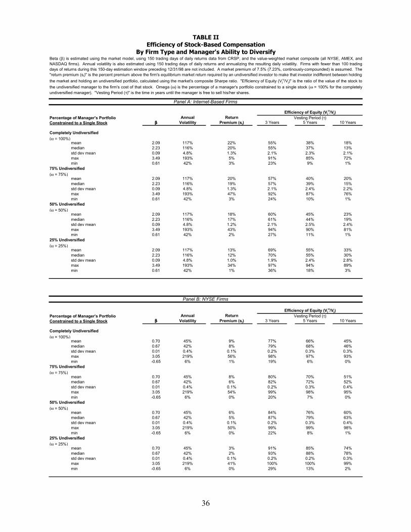
36

Annual Returnββββ Volatility Premium (sj) 3 Years 5 Years 10 Years

Completely Undiversified(ω = 100%)

mean 2.09 117% 22% 55% 38% 18%median 2.23 116% 20% 55% 37% 13%std dev mean 0.09 4.8% 1.3% 2.1% 2.3% 2.1%max 3.49 193% 5% 91% 85% 72%min 0.61 42% 3% 23% 9% 1%

75% Undiversified(ω = 75%)






the market and holding an undiversified portfolio, calculated using the market's composite Sharpe ratio. "Efficiency of Equity (Vju/Vj)" is the ratio of the value of the stock to

the undiversified manager to the firm's cost of that stock. Omega (ω) is the percentage of a manager's portfolio constrained to a single stock (ω = 100% for the completelyundiversified manager). "Vesting Period (τ)" is the time in years until the manager is free to sell his/her shares.

Constrained to a Single Stock

Panel A: Internet-Based Firms

Efficiency of Equity (Vju/Vj)

Vesting Period (τ)Percentage of Manager's Portfolio

TABLE IIEfficiency of Stock-Based Compensation

By Firm Type and Manager's Ability to DiversifyBeta (β) is estimated using the market model, using 150 trading days of daily returns data from CRSP, and the value-weighted market composite (all NYSE, AMEX, andNASDAQ firms). Annual volatility is also estimated using 150 trading days of daily returns and annualizing the resulting daily volatility. Firms with fewer than 100 tradingdays of returns during this 150-day estimation window preceding 12/31/98 are not included. A market premium of 7.5% (7.23%, continously-compounded) is assumed. The"return premium (sj)" is the percent premium above the firm's equilibrium market return required by an undiversified investor to make that investor indifferent between holding



mean 0.70 45% 9% 77% 66% 45%median 0.67 42% 8% 79% 68% 46%std dev mean 0.01 0.4% 0.1% 0.2% 0.3% 0.3%max 3.05 219% 56% 98% 97% 93%min -0.65 6% 1% 19% 6% 0%







Constrained to a Single StockPercentage of Manager's Portfolio

Panel B: NYSE Firms


Vesting Period (τ)

37



TABLE II (cont.)Efficiency of Stock-Based Compensation












Panel C: AMEX Firms


Vesting Period (τ)











Panel D: NASDAQ Firms


Vesting Period (τ)

38



TABLE II (cont.)Efficiency of Stock-Based Compensation












Panel E: All Firms


Vesting Period (τ)

39

Annual Returnββββ Volatility Premium(sj) 3 Years 5 Years 10 Years

Completely Undiversified(ω = 1.00)


75% Undiversified(ω = .75)






Constrained to a Single Stock

Beta (β) is estimated using the market model, using 150 trading days of daily returns data from CRSP, and the value-weighted market composite (all NYSE, AMEX, andNASDAQ firms). Annual volatility is also estimated using 150 trading days of daily returns and annualizing the resulting daily volatility. Firms with fewer than 100 tradingdays of returns during this 150-day estimation window preceding 12/31/98 are not included. A market premium of 7.5% (7.23%, continously-compounded) is assumed. The"return premium (sj)" is the percent premium above the firm's equilibrium market return required by an undiversified investor to make that investor indifferent between holding the market and holding an undiversified portfolio, calculated using the market's composite Sharpe ratio. "Efficiency of Options" is the ratio between the value of the stockoptions to the partially-diversified manager to the firm's cost of those stock options. The Balck-Scholes option pricing formula is used to price the options. The divident yieldis assumed to be zero. Omega (ω) is the percentage of a manager's portfolio constrained to a single stock (ω = 100% for the completely undiversified manager). "VestingPeriod (τ)" is the time in years until the manager is free to sell his/her shares.

Vesting Period (τ)Option Efficiency for 10-Year Options

By Firm Type and Manager's Ability to DiversifyEfficiency of Option-Based Compensation

Percentage of Manager's Portfolio

TABLE III

Panel A: Internet-Based Firms










Panel B: NYSE Firms


Option Efficiency Based Upon Maturity of OptionVesting Period (τ)

40











TABLE III (cont.)Efficiency of Option-Based Compensation

By Firm Type and Manager's Ability to DiversifyBeta (β) is estimated using the market model, using 150 trading days of daily returns data from CRSP, and the value-weighted market composite (all NYSE, AMEX, andNASDAQ firms). Annual volatility is also estimated using 150 trading days of daily returns and annualizing the resulting daily volatility. Firms with fewer than 100 tradingdays of returns during this 150-day estimation window preceding 12/31/98 are not included. A market premium of 7.5% (7.23%, continously-compounded) is assumed. The"return premium (sj)" is the percent premium above the firm's equilibrium market return required by an undiversified investor to make that investor indifferent between holding the market and holding an undiversified portfolio, calculated using the market's composite Sharpe ratio. "Efficiency of Options" is the ratio between the value of the stockoptions to the partially-diversified manager to the firm's cost of those stock options. The Black-Scholes option pricing formula is used to price the options. The divident yieldis assumed to be zero. Omega (ω) is the percentage of a manager's portfolio constrained to a single stock (ω = 100% for the completely undiversified manager). "VestingPeriod (τ)" is the time in years until the manager is free to sell his/her shares.

Panel C: AMEX Firms











Panel D: NASDAQ Firms



41











TABLE III (cont.)Efficiency of Option-Based Compensation

By Firm Type and Manager's Ability to DiversifyBeta (β) is estimated using the market model, using 150 trading days of daily returns data from CRSP, and the value-weighted market composite (all NYSE, AMEX, andNASDAQ firms). Annual volatility is also estimated using 150 trading days of daily returns and annualizing the resulting daily volatility. Firms with fewer than 100 tradingdays of returns during this 150-day estimation window preceding 12/31/98 are not included. A market premium of 7.5% (7.23%, continously-compounded) is assumed. The"return premium (sj)" is the percent premium above the firm's equilibrium market return required by an undiversified investor to make that investor indifferent between holding the market and holding an undiversified portfolio, calculated using the market's composite Sharpe ratio. "Efficiency of Options" is the ratio between the value of the stockoptions to the partially-diversified manager to the firm's cost of those stock options. The Black-Scholes option pricing formula is used to price the options. The divident yieldis assumed to be zero. Omega (ω) is the percentage of a manager's portfolio constrained to a single stock (ω = 100% for the completely undiversified manager). "VestingPeriod (τ)" is the time in years until the manager is free to sell his/her shares.

Panel E: All Firms


42

COM

PANY

BY

CLAS

SIFI

CATI

ON

Valu

e of

Equ

ity ($

milli

ons)

Valu

e of

Equ

ity ($

milli

ons)

COM

MER

CE T

ECHN

OLO

GIE

S &

SERV

ICES

CONT

ENT

SERV

ICES

AMAZ

ON

COM

INC

16,9

50AM

ERIC

A O

NLIN

E IN

C71

,070

BEYO

ND C

OM

CO

RP10

4BR

OAD

CAST

CO

M IN

C1,

308

CDNO

W IN

C31

8C

M G

I IN

C2,

458

CEND

ANT

CORP

16,4

75C

N E

T IN

C90

5CH

ECKF

REE

HOLD

ING

S CO

RP1,

216

EXCI

TE IN

C2,

215

CYBE

RCAS

H IN

C23

6G

EOCI

TIES

1,05

8CY

BERI

AN O

UTPO

ST IN

C60

7IN

FOSE

EK C

ORP

1,55

6DO

UBLE

CLIC

K IN

C74

0IN

TUIT

INC

4,33

7E

TRAD

E G

ROUP

INC

2,65

5LY

COS

INC

2,38

6EB

AY IN

C9,

714

SPO

RTSL

INE

USA

INC

298

EGG

HEAD

CO

M IN

C51

5TH

EGLO

BE C

OM

102

NETW

ORK

SO

LUTI

ONS

INC

545

TICK

ETM

ASTE

R O

NLIN

E CI

TYSR

CH IN

C39

2O

NSAL

E IN

C76

9YA

HOO

INC

23,3

84PE

APO

D IN

C11

7PR

EVIE

W T

RAVE

L IN

C25

0IN

TERN

ET S

OFT

WAR

EST

ERLI

NG C

OM

MER

CE IN

C4,

255

UBID

INC

168

BRO

ADVI

SIO

N IN

C78

6XO

OM

CO

M IN

C13

2EA

RTHW

EB IN

C82

INKT

OM

I CO

RP3,

213

COM

MUN

ICAT

IONS

TEC

HNO

LOG

IES

& SE

RVIC

ESM

ICRO

SOFT

CO

RP34

2,55

8NE

TGRA

VITY

INC

227

24 7

MED

IA IN

C43

4NE

TSCA

PE C

OM

MUN

ICAT

IONS

CO

RP6,

046

ASCE

ND C

OM

MUN

ICAT

IONS

INC

14,2

63O

PEN

MAR

KET

INC

409

AT H

OM

E CO

RPO

RATI

ON

9,15

3RE

ALNE

TWO

RKS

INC

1,08

0CI

SCO

SYS

TEM

S IN

C14

5,99

4SP

YGLA

SS IN

C33

0CI

TRIX

SYS

TEM

S IN

C4,

139

SUN

MIC

ROSY

STEM

S IN

C32

,988

EART

HLIN

K NE

TWO

RK IN

C1,

626

VERI

SIG

N IN

C1,

365

EXO

DUS

COM

MUN

ICAT

IONS

INC

1,30

3M

INDS

PRIN

G E

NTER

PRIS

ES IN

C1,

585

SECU

RITY

N2K

INC

186

PSIN

ET IN

C1,

082

AXEN

T TE

CHNO

LOG

IES

INC

760

USW

EB C

ORP

1,20

1NE

TWO

RKS

ASSO

CIAT

ES IN

C8,

950

VERI

O IN

C73

7SE

CURI

TY D

YNAM

ICS

TECH

S IN

C95

3

APPE

NDIX

BCo

mpo

sitio

n of

Ham

brec

ht &

Qui

st's

(H&Q

) Ind

ex o

f Int

erne

t-Bas

ed F

irms

By B

usin

ess

Desc

riptio

n, a

s of

Dec

embe

r 31,

199

8

43

ANNUAL STOCK RETURN EFFICIENCYCOMPANY ββββ VOLATILITY PRICE ($) PREMIUM (sj) OF EQUITY EXP. IN 3 YRS EXP. IN 10 YRS24 7 MEDIA INC 3.23 171% 28 30% 40% 37% 40%AMAZON COM INC 2.20 110% 321 1/4 19% 57% 49% 56%AMERICA ONLINE INC 1.90 70% 155 1/8 8% 78% 67% 75%ASCEND COMMUNICATIONS INC 1.55 64% 65 3/4 9% 77% 64% 73%AT HOME CORPORATION 2.30 97% 74 1/4 14% 66% 57% 64%AXENT TECHNOLOGIES INC 1.68 78% 30 9/16 12% 69% 57% 66%BEYOND COM CORP 2.44 135% 20 3/4 25% 48% 42% 47%BOUNDLESS CORP 0.82 111% 5 29% 42% 32% 40%BROADCAST COM INC 2.33 125% 76 1/2 22% 51% 44% 50%BROADVISION INC 1.34 118% 32 27% 44% 36% 43%C M G I INC 3.49 125% 106 1/2 14% 65% 60% 65%C N E T INC 2.04 120% 53 1/4 23% 50% 43% 49%CDNOW INC 2.61 155% 18 30% 41% 36% 41%CENDANT CORP 1.70 86% 19 5/16 15% 64% 53% 62%CHECKFREE HOLDINGS CORP 1.72 119% 23 3/8 25% 47% 40% 46%CISCO SYSTEMS INC 1.70 53% 92 13/16 4% 88% 78% 84%CITRIX SYSTEMS INC 1.66 61% 97 1/16 7% 81% 69% 77%CYBERCASH INC 1.59 121% 15 26% 45% 37% 44%CYBERIAN OUTPOST INC 2.88 193% 27 1/2 40% 30% 28% 30%CYLINK CORP 1.16 183% 3 5/8 49% 23% 20% 23%DIALOG CORP 0.71 106% 4 1/2 28% 43% 33% 41%DOUBLECLICK INC 2.64 125% 44 1/2 20% 55% 48% 54%E TRADE GROUP INC 2.20 114% 46 25/32 20% 55% 47% 54%EARTHLINK NETWORK INC 2.36 114% 57 19% 57% 50% 56%EBAY INC 2.51 164% 241 1/4 34% 37% 33% 36%EDIFY CORP 1.22 93% 8 5/16 20% 54% 43% 52%EGGHEAD COM INC 2.84 190% 20 13/16 39% 31% 29% 31%EXCITE INC 2.68 115% 42 1/16 17% 60% 53% 59%EXODUS COMMUNICATIONS INC 1.87 103% 64 1/4 19% 57% 47% 55%GEOCITIES 3.29 140% 33 5/8 20% 55% 50% 54%INFOSEEK CORP 2.20 108% 49 3/8 18% 58% 50% 57%INKTOMI CORP 2.39 133% 129 3/8 24% 48% 42% 47%INTUIT INC 2.37 80% 72 1/2 8% 78% 70% 76%ISS GROUP INC 1.54 97% 55 19% 56% 45% 54%LYCOS INC 2.96 116% 55 9/16 15% 64% 57% 63%MICROSOFT CORP 1.38 42% 138 11/16 3% 91% 81% 87%MINDSPRING ENTERPRISES INC 2.39 107% 61 1/16 16% 61% 53% 60%N2K INC 1.84 167% 13 1/16 39% 31% 27% 31%NETGRAVITY INC 3.31 173% 16 3/4 30% 40% 37% 40%NETSCAPE COMMUNICATIONS CORP 2.68 118% 60 3/4 18% 59% 52% 58%NETWORK SOLUTIONS INC 2.25 124% 130 7/8 23% 50% 44% 50%NETWORKS ASSOCIATES INC 1.45 63% 66 1/4 9% 76% 62% 72%NEWSEDGE CORP 0.61 157% 11 5/8 45% 26% 22% 26%ONSALE INC 3.11 185% 40 1/16 36% 34% 32% 34%OPEN MARKET INC 2.64 184% 11 11/16 39% 31% 29% 31%PEAPOD INC 1.31 132% 6 13/16 32% 38% 32% 38%PREVIEW TRAVEL INC 2.99 141% 18 7/16 23% 50% 45% 50%PSINET INC 2.25 99% 20 7/8 15% 64% 55% 62%REALNETWORKS INC 2.41 125% 35 7/8 22% 52% 45% 51%SECURITY DYNAMICS TECHS INC 2.35 108% 23 17% 60% 52% 59%SPORTSLINE USA INC 1.46 129% 15 9/16 30% 41% 34% 40%SPYGLASS INC 2.31 107% 22 17% 60% 52% 59%STERLING COMMERCE INC 1.25 72% 45 14% 67% 52% 63%SUN MICROSYSTEMS INC 1.35 53% 85 5/8 7% 82% 68% 77%USWEB CORP 2.34 119% 26 3/8 21% 54% 47% 53%VERIO INC 1.60 108% 22 3/8 22% 51% 42% 49%VERISIGN INC 1.33 84% 59 1/8 17% 60% 48% 57%YAHOO INC 2.37 85% 236 15/16 10% 75% 66% 73%

Internet Firms: Efficiency of Stock and Option-Based CompensationPaid to Executives with Completely Undiversified Investment Portfolios

APPENDIX C

EFFICIENCY OF OPTIONS

Beta (β) estimated with 150 days of daily returns (ending 12/31/98) and the value-weighted market composite market index. Firms with fewer than 42 days of returns during thiswindow were dropped. Return premium (sj) is the expected return needed to made an undiversified manager indifferent between holding a single-stack portfolio of her firm'sstock and holding a market porfoltio levered to an equivalent volatility level. Efficiency of Equity (Vju/Vj) equals the value of the stock to an undiversified investor divided bymarket value. Efficiency of Options is the value of an option to an undiversified manager divided by the market value of the option. The assumed market risk premium is 7.5%.Uses the Black-Scholes option-pricing model, assuming no dividends. Vesting period equals 3 years.

44

References

Abowd, J. M. and D. S. Kaplan, 1999, "Executive Compensation: Six Questions ThatNeed Answering," NBER Working Paper Series #7124 (May 1999).

Acharya, V. V., K. John and R. K. Sindaram, 2000, "On the Optimality of ResettingExecutive Stock Options," Journal of Financial Economics 57 (1), 65-101.

Aggarwal, R. K. and A. A. Samwick, 1999, "The Other Side of the Trade-Off: TheImpact of Risk on Executive Compensation," Journal of Political Economy 107 (1), 65-105.

Black, F. and M. Scholes, 1973, "The Pricing of Options and Corporate Liabilities,"Journal of Political Economy 81 (May-June), 637-654.

Boczar, T. J., 1998, "Stock Concentration Risk Management after Tra '97; TaxpayerRelief Act of 1997," Trusts and Estates 137 (4), 45.

Bolster, P., D. Chance and D. Rich, 1986, "Executive Equity Swaps and CorporateInsider Holdings," Financial Management 25 (2), 14-24.

Brenner, M., R. K. Sundaram and D. Yermack, 2000, "Altering the Terms of ExecutiveStock Options," Journal of Financial Economics 57 (1), 103-128.

Campbell, J. Y., M. Lettau, B. G. Malkiel and Y. Xu, 2001, "Have Individual StocksBecome More Volatile? An Empirical Exploration of Idiosyncratic Risk," Journal of FinanceLVI (1), 1-43.

Carpenter, J. N., 1998, "The Exercise and Valuation of Executive Stock Options,"Journal of Financial Economics 48 (2), 127-158.

Carpenter, J. N., 2000, "Does Option Compensation Increase Managerial RiskAppetite?," Journal of Finance 55 (5), 2311-2332.

Carpenter, J. N. and B. Remmers, 2000, "Executive Stock Option Exercises and insideInformation," NYU Stern School of Business Working Paper.

Chance, D. M., R. Kumar and R. B. Todd, 2000, "The "Repricing" of Executive StockOptions," Journal of Financial Economics 57 (1), 129-154.

Cohen, R. B., B. J. Hall and L. M. Viceira, 2000, "Do Executive Stock OptionsEncourage Risk Taking?," Harvard Business School Working Paper.

Core, J. E. and D. F. Larcker, 2000, "Performance Consequences of Mandatory Increasesin Ceo Stock Ownership," Working Paper Series (July 3, 2000).

45

Cuny, C. J. and P. Jorion, 1995, "Valuing Executive Stock Options with EndogenousDeparture," Journal of Accounting and Economics 20, 193-205.

Dechow, P. M., A. P. Hutton and R. G. Sloan, 1997, "Economic Consequences ofAccounting for Stock-Based Compensation," Journal of Accounting Research 34 (Supplement1996).

DeFusco, R. A., T. S. Zorn and R. R. Johnson, 1991, "The Association betweenExecutive Stock Option Plan Changes and Managerial Decision Making," FinancialManagement 20 (1), 36-43.

Degeorge, F., D. Jenter, A. Moel and P. Tufano, 2000, "Selling Company Shares toReluctant Employees: France Telecom's Experience," Harvard Business School Working PaperSeries (May 18, 2000).

Detemple, J. and S. Sundaresan, 1999, "Nontraded Asset Valuation with PortfolioConstraints: A Binomial Approach," The Review of Financial Studies 12 (4), 835-872.

Fama, E. F. and K. R. French, 1992, "The Cross-Section of Expected Stock Returns,"Journal of Finance 46, 427-465.

Friend, I. and M. E. Blume, 1975, "The Demand for Risky Assets," American EconomicReview 65 (5), 901-922.

Gaver, J. J. and K. M. Gaver, 1995, "Compensation Policy and the InvestmentOpportunity Set," Financial Management 24 (1), 19-32.

Gilson, S. C. and M. R. Vestuypens, 1993, "Ceo Compensation in Financially DistressedFirms: An Empirical Analysis," Journal of Finance 48 (2), 425-458.

Hall, B. J. and J. B. Liebman, 1998, "Are Ceos Really Paid Like Bureaucrats?," TheQuarterly Journal of Economics 113 (3), 653-691.

Hall, B. J. and K. J. Murphy, 2000a, "Optimal Excercise Prices for Executive StockOptions," American Economic Review 90 (2), 209-214.

Hall, B. J. and K. J. Murphy, 2000b, "Stock Options for Undiversifed Executives,"Working Paper (October 2000).

Haugen, R. A. and L. W. Senbet, 1981, "Resolving the Agency Problems of ExternalCapital through Options," Journal of Finance 36 (3), 629-647.

Huddart, S., 1994, "Employee Stock Options," Journal of Accounting and Economics 18,207-231.

46

Huddart, S. and M. Lang, 1996, "Employee Stock Option Exercises: An EmpiricalAnalysis," Journal of Accounting and Economics 21 (1), 5-43.

Hull, J. C. and A. White, 1987, "The Pricing of Options on Assets with StochasticVolatilities," Journal of Finance 42 (June), 281-300.

Jensen, M. C. and K. J. Murphy, 1990, "Performance Pay and Top-ManagementIncentives," Journal of Political Economy 98 (2).

Jin, L., 2000, Ceo Compensation, Risk Sharing, and Incentives: Theory and EmpiricalResults, Sloan School of Management, Massachusetts Institute of Technology.

Johnson, H. and D. Shanno, 1987, "Option Pricing When the Variance Is Changing,"Journal of Financial and Quantitative Analysis 22 (2), 143-152.

Johnson, S. A. and Y. S. Tian, 2000, "The Value and Incentive Effects of NontraditionalExecutive Stock Option Plans," Journal of Financial Economics 57 (1), 3-34.

Kulatilaka, N. and A. J. Marcus, 1994, "Valuing Employee Stock Options," FinancialAnalysts Journal 50 (6), 46-56.

Lambert, R. A. and D. F. Larcker, 1988, "An Analysis of the Use of Accounting andMarket Measures of Performance in Executive Compensation Contracts," Journal of AccountingResearch 25 (Supplement 1987), 85-125.

Lambert, R. A., D. F. Larcker and R. E. Verrecchia, 1991, "Portfolio Considerations inValuing Executive Compensation," Journal of Accounting Research 29 (1), 129-149.

Larcker, D. F., 1983, "The Association between Performance Plan Adoption andCorporate Capital Investment," Journal of Accounting and Economics 5 (1), 3-31.

Long, M. S., 1992, "The Incentives Behind the Adoption of Executive Stock OptionPlans in U.S. Corporations," Financial Management 21 (3), 12-21.

McConaughy, D. L. and C. S. Misha, 1996, "Debt, Performance-Based Incentives, andFirm Performance," Financial Management 25 (2), 37-51.

Merton, R. C., 1992, Continuous-Time Finance, Cambridge, MA, Blackwell.

Meulbroek, L. K., 2000a, "Does Risk Matter? Corporate Insider Transations in Internet-Based Firms," Harvard Business School Working Paper 00-062.

Meulbroek, L. K., 2000b, "Executive Compensation Based Upon Relative Performance:Are Indexed Stock Options More Efficient?," Harvard Business School Working Paper 01-021(December, 2000).

47

Murphy, K. J., 1985, "Corporate Performance and Managerial Remuneration: AnEmpirical Analysis," Journal of Accounting and Economics 7 (1-3), 11-43.

Murphy, K. J., 1998, "Executive Compensation," in O. Ashenfelter and D. Card, Ed.,Handbook of Labor Economics, Amsterdam, North-Holland.

Ofek, E. and D. Yermack, 2000, "Taking Stock: Equity-Based Compensation and theEvolution of Managerial Ownership," Journal of Finance 55 (3), 1367 - 1384.

Rajgopal, S. and T. Shevlin, 1999, "Stock Option Compensation and Risk Taking: TheCase of Oil and Gas Producers," Working Paper (July 1999).

Ross, S. A., 1976, "Arbitrage Theory of Capital Asset Pricing," Journal Of EconomicTheory 13, 341-360.

Schizer, D. M., 2000, "Executives and Hedging: The Fragile Legal Foundation ofIncentive Compatability," Columbia Law Review 100 (2), 440-504.

Smith, C. and R. Watts, 1992, "The Investment Opportunity Set and CorporateFinancing, Dividend, and Compensation Policies," Journal of Financial Economics 32, 263-292.

Smith, C. W. and J. L. Zimmerman, 1976, "Valuing Employee Stock Option Plans UsingOption Pricing Models," Journal of Accounting Research, 357-364.

Wiggins, J. B., 1987, "Options Values under Stochastic Volatility: Theory and EmpiricalEstimates," Journal of Financial Economics 19 (2), 351-373.

Yermack, D., 1995, "Do Corporations Award Ceo Stock Options Effectively?," Journalof Financial Economics 39, 237-269.

the efficiency of equity- linked compensation ... files/00-056_26efecae-5cf8-4b4a... · 3...

Documents