the effects of open enrollment on school choice and

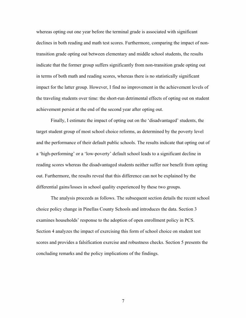
The Effects of

Open Enrollment on

School Choice and

Student Outcomes

UmUt Özek

w o r k i n g p a p e r 2 6 • m a y 2 0 0 9

The Effects of Open Enrollment on School Choice and Student Outcomes

Umut Özek University of Florida

The author thanks the School Board of Pinellas County for providing the data; David Figlio, Richard Romano, Lawrence Kenny, Sarah Hamersma, Jonathan Hamilton, Steven Slutsky, David Sappington; seminar participants at the University of North Carolina at Greensboro, University of Oregon, University of Oklahoma, RAND Corporation and the Urban Institute for useful comments; and Burak Özek for excellent research assistance. The author gratefully acknowledges support from the National Science Foundation and the National Center for the Analysis of Longitudinal Data in Education Research (CALDER), supported by Grant R305A060018 to the Urban Institute from the Institute of Education Sciences, U.S. Department of Education. The views expressed are those of the author and may not reflect those of the funders or institutions. Any errors are attributable to the author. CALDER working papers have not gone through final formal review and should be cited as working papers. They are intended to encourage discussion and suggestions for revision before final publication.

CONTENTS

Introduction 1 Policy Background and Data Description 8

Policy Background 8 Data Description 10

Impact of Open Enrollment on School Choice 13 Incidence of Opting Out 13 Composition of Opt-Out Students 14

Opting Out and Student Test Scores 15 Where Do Students Opt Out? 16 Ordinary Least Squares (OLS) Results 18 IV Results 19 Disentangling the Reasons Underlying the Detrimental Impact 24 Impact of Opting Out - Disadvantaged Students 27 Falsification Test 29 Robustness Checks 30

Concluding Remarks 30

References 33 Appendix 35

i

The Effects of Open Enrollment on School Choice and Student Outcomes Umut Özek CALDER Working Paper No. 26 May 2009

ABSTRACT

This paper analyzes households’ response to the introduction of intra-district school

choice and examines the impact of exercising this choice on student test scores in Pinellas

County Schools, one of the largest school districts in the United States. Households react

strongly to the incentives created by such programs, leading to significant changes in the

frequency of exercising alternative public schooling options, as well as changes in the

composition of the “opt out” students. However, using “proximity to public alternatives”

as an instrument for opting out of the “assigned” public school, the author finds no

significant benefit of opting out on student achievement. Also, the author finds those who

opt out of their default public schools often perform significantly worse on standardized

tests than similar students who stay behind. Results suggest that the short-run detrimental

effects of opting out are stronger for students who opt out closer to the terminal grade of

the school level, yet weaker for “disadvantaged” students, who typically constitute the

proposed target of school choice reforms.

ii

The Effects of Open Enrollment on School Choice and Student Outcomes

1. Introduction

Improving the quality of elementary and secondary education remains atop the

political agenda in the United States, which annually spends roughly 1.5 times more

money per pupil on primary and secondary education than the average member of the

Organization for Economic Cooperation and Development (OECD) 1. Yet, the additional

resources allocated to education do not fully translate into higher student achievement:

the U.S. students perform worse than the OECD averages on international tests in math,

reading and science2.

Increasing parental choice has been one of the leading themes of the educational

policy implemented to enhance academic achievement in the U.S. during the last two

decades. The main objective of such policies is to ‘level the playing field’ in terms of

access to quality education for disadvantaged students who cannot otherwise afford the

higher-quality schooling options. Along these lines, open enrollment programs such as

inter-district and intra-district school choice, which allow parents to send their children to

public schools outside of the neighborhoods in which they reside, have become

increasingly popular. As of 2005, 27 states had passed legislation mandating school

districts to implement intra-district school choice, and 20 states had adopted legislation

mandating that school districts participate in the inter-district choice program of their

state (ECS, 2005). There is also an increasing trend in the percentage of households

1 OECD (2008). In 2004, the per-pupil spending on primary (secondary) education in the U.S. was $9,156 ($10,390) compared to the OECD average of $6,252 ($7,804). 2 OECD (2003). In 2003, as part of the Programme for International Student Assessment (PISA), OECD tested the 8th graders in member countries on subjects including math, reading and science. The average test scores for U.S. students were 483, 491 and 495 in math, science and reading respectively compared to OECD averages of 500, 499 and 494.

1

participating in open enrollment programs. Between 1993 and 2003, the percentage of

students attending a public school other than their neighborhood schools increased from

11 percent to 15.4 percent in the United States (NCES, 2006).

This study analyzes households’ response to the introduction of public school

choice in the form of open enrollment in Pinellas County Schools (PCS), one of the

largest school districts in the U.S., and examines the impact of exercising this form of

school choice on student test scores. Having abandoned the zoning regime with court-

ordered busing, which had been used to prevent racial segregation for more than three

decades, and implemented intra-district school choice in 2003, PCS provides an

appealing case to analyze the impact of increased educational opportunities on

households’ school choice behavior3,4.

Using the entire elementary and middle school student population attending 4th

through 8th grades between 2001 and 2005 in PCS, the results indicate that households

reacted strongly to the incentives created by the open enrollment program, leading to

significant increases in the rate of students who opt out of their default schools. Among

the transition-grade students (6th graders who transitioned from elementary school to

middle school at the beginning of the school year), the implementation of open

enrollment increased the percentage of students who opt out of their default middle

3 The introduction of open enrollment expanded the feasible public school choice for the majority of public school students in PCS whereas it changed, but not necessarily expanded, the set of relevant choices for those who were able to attend public schools other than their ‘neighborhood’ public schools prior to the policy change with the use of Special Attendance Permits. The following section describes this policy change in more detail. 4 In the U.S. context, the focus of the previous literature has been mainly on the impact of increased public school choice on student outcomes and households’ school choice in a regime where school choice has already been introduced. See Cullen, Jacob and Levitt (2005, 2006); Hastings, Kane and Staiger (2008). There are several exceptions in the international context though. An important example is Fiske and Ladd (2000), who examine the impact of a dramatic school choice reform on households’ behavior in New Zealand.

2

school from 8 percent to 33 percent, whereas for non-transition grade students, the opt

out rate increased from 7 percent to 16 percent in the year following policy adoption. The

findings also reveal significant changes in the composition of opt out students following

the policy change. The implementation of open enrollment, by reducing the implicit cost

of opting out for students, ‘smoothed-out’ the prior achievement levels of the traveling

students, attracting more mediocre students to opt out.

Having established that households responded to the incentives created by the

open enrollment program, I then examine the impact of exercising this form of school

choice on test scores. By expanding the set of feasible public schools available to each

household, open enrollment programs might enhance student achievement in two ways.

First, students, who cannot otherwise afford higher quality schooling options, might be

able to attend higher quality public schools or schools that better match their interests and

needs under the open enrollment regime. Furthermore, if the increasing competition

among public schools improves the efficiency of the public provision of education, open

enrollment programs will enhance student achievement by increasing the overall quality

of public education. The extent to which open enrollment improves student achievement

relies on households’ willingness and ability to send their children to higher quality

public schools in the presence of open enrollment5.

However, testing these predictions has been proven difficult due to the highly

selective nature of opting out. In other words, if those who opt out of their default public

5 In the ideal setting, absent frictions, open enrollment programs allow parents to send their children to any public school within the boundaries of a region that contains, but is not limited to, the household’s neighborhood. However, in practice, parents are typically limited in their public school choices by non-boundary constraints, especially public school capacities, restricting households’ ability to send their children to higher quality public schools. Furthermore, households might place more weight on non-academic characteristics of public schools such as proximity, limiting the competitive pressure public schools face under open enrollment (Hastings, Kane and Staiger, 2008).

3

schools differ from their peers who stay behind along unobservable characteristics such

as ‘intrinsic motivation to excel’, traditional ordinary least-squares approach fails to

provide unbiased estimates of the causal relationship between opting out and student

achievement. A recent body of research makes use of randomized lotteries, which are

commonly employed by school districts and schools to determine the assignments in

oversubscribed public schools, to deal with this issue6. Comparing the student outcomes

between the lottery-winners and lottery-losers, these studies typically find no significant

benefit of attending selective public schools on student test scores7. However, these

estimates will not necessarily reflect the true impact of exercising the school choice

provided by open enrollment on student outcomes for the entire student body if those

who participate in lotteries differ from the entire student population8.

Cullen, Jacob and Levitt (2005), on the other hand, employ instrumental variables

approach to estimate the causal relationship between opting out of the assigned public

school and student outcomes. Using ‘proximity to the closest public alternative’ as an

instrument for opting out, their results reveal that, other than for students who opt out to

high school career academies, there is no significant impact of opting out of the

6 Some examples in the open enrollment context are Cullen, Jacob and Levitt (2006); Cullen and Jacob (forthcoming); Hastings, Kane and Staiger (2008). Hastings and Weinstein (forthcoming), on the other hand, use natural and field experiments in which some parents are randomly provided information about school quality. They find that those who receive the information are more likely to send their children to higher quality schools and those who attend higher quality schools perform better on standardized tests. 7 Even though no significant effect of winning the lottery on the average lottery participant is the main conclusion of all these studies, some studies find significant benefits of opting out for certain subgroups. For instance, Hastings, Kane and Staiger (2008) find that children of parents with strong preference for academic quality experience significant gains in test scores as a result of attending their chosen school, while children whose parents weighted academic characteristics less heavily experience academic losses. 8 Randomized lotteries become necessary when there are more applicants than the number of seats available at a given school. If the demand for a public school is correlated with the school’s quality, then lotteries will take place more frequently at higher quality public schools. Therefore, it is quite likely that the lottery participants have higher tastes for quality education than non-participants.

4

‘assigned’ high school at the end of 8th (transition) grade on the probability of dropping-

out during the high school years.

Using ‘proximity to the ‘relevant’ public alternatives’ as an instrument for opting

out of the default public school, I estimate the impact of opting out on student test scores

for elementary and middle school students between grades 4 and 8. Despite the similar

use of ‘proximity’ for identification, this study extends Cullen, Jacob and Levitt (2005)

along two important dimensions. First, I am able to use test scores as the outcome of

interest, since I eliminate the selection problem caused by drop-outs by excluding high

school students. Moreover, the findings presented in this paper provide a more complete

picture about the impact of exercising this form of school choice on student outcomes,

since the dataset I employ enables me to analyze the impact of ‘non-transition grade

opting out’ as well as ‘transition grade opting out’ on test scores.

The findings reveal no significant benefit of opting out on student test scores and

that the students who opt out of their default schools often perform significantly worse in

reading than similar students who stay: the average traveling student scores roughly one-

quarter of a standard deviation lower in reading. Given the substantially different nature

of opting out for transition grade students and non-transition grade students, I further

disaggregate the analysis into these two groups. The IV analysis on the two sub-samples

indicate that the detrimental impact of opting out on reading scores for the entire sample

is mainly driven by the non-transition graders. The transition-grade students, on the other

hand, neither bear any significant costs nor benefit from opting out of their assigned

middle schools.

5

There are several competing mechanisms through which opting out might affect

student achievement in a negative way. One explanation is that frictions such as binding

public school capacity constraints limit the ability of those who opt out to exercise higher

quality schooling options. Comparisons between the default and target schools during the

school year before the opt-out reveal that the traveling students did not experience

significant changes in school quality compared to their peers who stayed behind in our

sample.9 Moreover, opting out might have deteriorating effects on traveling students’

achievement levels if being an outsider at the new school leads to a decline in the

intrinsic motivation of the students.

A direct implication of the ‘outsider effect’ is that those who opt out closer to the

terminal grade of the school level will experience higher achievement losses, since the

lack of time and incentives to become an ‘insider’ might translate into more severe

declines in intrinsic motivation. Similarly, keeping the proximity to the terminal grade of

the school level constant, elementary school students are expected to suffer more from

non-transition grade opting out, since their new peers at the target school are likely to

have spent more time together, making it harder for the traveling students to become

insiders. Finally, if ‘getting used to the new school environment’ is positively correlated

with students’ intrinsic motivation, one would expect to see an improvement in student

achievement at the end of the second year after opting out.

The results provide evidence supporting the first two implications of the

‘outsider’ effect: those who opt out two years before the terminal grade of the school

level benefit significantly (one-third of the standard deviation) in terms of math scores

9 For instance, the average gain in teacher experience for the traveling students is 0.1 years, whereas the average teacher experience in the entire sample is 13.2 years.

6

whereas opting out one year before the terminal grade is associated with significant

declines in both reading and math test scores. Furthermore, comparing the impact of non-

transition grade opting out between elementary and middle school students, the results

indicate that the former group suffers significantly from non-transition grade opting out

in terms of both math and reading scores, whereas there is no statistically significant

impact for the latter group. However, I find no improvement in the achievement levels of

the traveling students over time: the short-run detrimental effects of opting out on student

achievement persist at the end of the second year after opting out.

Finally, I estimate the impact of opting out on the ‘disadvantaged’ students, the

target student group of most school choice reforms, as determined by the poverty level

and the performance of their default public schools. The results indicate that opting out of

a ‘high-performing’ or a ‘low-poverty’ default school leads to a significant decline in

reading scores whereas the disadvantaged students neither suffer nor benefit from opting

out. Furthermore, the results reveal that this difference can not be explained by the

differential gains/losses in school quality experienced by these two groups.

The analysis proceeds as follows. The subsequent section details the recent school

choice policy change in Pinellas County Schools and introduces the data. Section 3

examines households’ response to the adoption of open enrollment policy in PCS.

Section 4 analyzes the impact of exercising this form of school choice on student test

scores and provides a falsification exercise and robustness checks. Section 5 presents the

concluding remarks and the policy implications of the findings.

7

2. Policy Background and Data Description

2.1. Policy Background

In order to examine the impacts of increasing public school choice, I use the

recent school-choice policy change in one of the largest school districts in the U.S.,

Pinellas County Schools (PCS), which adopted its intra-district choice program in 2003.

Prior to open enrollment, for over three decades, public school assignments in the district

were determined using a zoning regime with ‘forced’ busing, under which households’

residential choices had direct implications on the public school their children will attend;

however, a minority of students was forced to attend other public schools to avoid racial

segregation. Students could also voluntarily opt out of their default schools using Special

Attendance Permits (SAP)10. During the pre-policy period, the majority of the students

who attended a public school other than their ‘zoned’ schools were in the latter category:

during the 1999-2000 school year, 6,048 (5.3%) out of the 114,500 enrolled students in

PCS were able to attend a different public school than their ‘zoned’ schools using

SAPs11.

Under the new school-choice regime, the school district is divided into four

attendance areas for elementary schools and three attendance areas for middle schools as

shown in Figures 1.1 and 1.2. The attendance areas at each grade level were determined

based on factors including population density, public school capacities and educational

10 Special Attendance Permit (SAP) grants students the privilege of attending a school in another attendance zone. Students are granted SAPs under extenuating circumstances including, but not limited to, child care needs, a family hardship or the medical condition of the child. Other factors including the racial diversity and the capacity of the ‘target’ school are also considered in processing SAP requests. 11 In the sample, prior to open enrollment, the rate of students who attended public schools other than their ‘zoned’ schools is roughly 6%, which implies that only 600 students were forced to opt-out in that school year. Given this evidence, I assume that all of the pre-policy opt-outs are voluntary throughout the remainder of the study, since the dataset I employ does not allow me to identify the bussed students during the pre-policy period.

8

offerings. ‘Non-traditional’ public schools including countywide fundamental schools,

magnet programs, charter schools and high school academies, each of which has a

separate application procedure and timeline, were excluded from this ‘choice’ plan12.

During the first year of the program, each student was required to submit a list of

her preferred schools, which could include any ‘traditional’ public school within the

boundaries of her attendance area, whereas in the subsequent years, only the transition-

grade students were required to submit their preferences.13 The non-transition graders

were automatically assigned to their current schools unless they submitted a list of their

preferences.

Given the submitted student preferences, if the number of applicants exceeded the

number of seats available at a given public school, assignments were determined using

the following priority categories and the assignment mechanism commonly referred to as

the ‘Boston’ mechanism14:

12 The main difference between countywide fundamental schools and ‘traditional’ public schools is that the former type admits any student in the district regardless of the residential location, depending on capacity constraints. 13 Prior to the introduction of open enrollment in PCS, Family Education and Information Centers (FEIC) were established to provide all parents information on school choice description and opportunities, available schools by attendance area, choice applications, transportation and school programs in order to assist them in choosing the appropriate schools for their children. As part of the ‘parent outreach’ program, FEIC staff was also required to visit libraries, day-care centers and community centers, and to speak to parent groups about the registration process and the academic programs. 14 Besides PCS, the Boston mechanism is also being used in some major school districts such as Cambridge, Charlotte, Denver, Hillsborough County, Miami-Dade County, Minneapolis and Seattle. Under the Boston mechanism, a student who is not assigned to his first choice is considered for his second choice only after the students who ranked that student’s second choice as their first choices. Thus, a student might lose her priority at a public school unless she lists that school as her first choice. One major issue with this assignment mechanism is that truthful revelation of public school preferences is not necessarily a weakly dominant strategy for households: it is not strategy-proof (Abdulkadiroglu and Sonmez, 2003).

9

1. Grandfathering and ‘Extended’ Grandfathering Priority

a. Continuation (Grandfathering) Priority: Allows students to remain at the

school of attendance until promotion to the next grade level or the student

otherwise leaves the school.

b. Extended Grandfathering Priority: Allows students to remain at the school

of attendance and progress through each school level previously assigned

to the parent/guardian’s address until the student graduates from high

school or the family moves out of the residence used to determine the

progression of schools15.

2. Family Priority: Used to assign family members to the same school where family

is defined as those who reside together as a family at the same address.

3. Proximity Priority: Provides increased likelihood that a family living closest to a

school will be selected to attend the school if that is the family’s first choice.

In the first step of the school choice plan called ‘controlled choice’ (2003-2007),

‘racial diversity’, which employs minimum and maximum racial percentages to ensure

diversity, was also used as an additional criterion for student assignments16.

2.2.Data Description

The data includes a panel of the entire PCS elementary and middle school

students attending 4th through 8th grades between 2001 and 2005. I exclude three types of

public school students from the analysis: high school students due to the sample selection 15 In other words, this preference allows students to stay at their ‘neighborhood schools’ to which they were assigned before the open enrollment program based on their residences. 16 For the years between 2003 and 2007, there were court-ordered ratios in place to help the district make the transition from the 1971 court order for desegregation to a unitary school system. During these four years, the maximum percentage of black students for any school was 42 percent. The minimum percentage of black students for a school was determined by the percentage of black students residing within each attendance area. Since the 2007-2008 school year, racial diversity has no longer been used to determine public school assignments.

10

issue created by students who drop-out; students attending non-traditional public schools

such as charter schools, magnet programs and countywide fundamental schools, since

these schools are not included in the PCS’s ‘choice program’; and students attending

kindergarten through 4th grade, since the standardized testing in PCS begins in the third

grade and I use previous year’s test score as a proxy for students’ intrinsic ability. These

restrictions result in 105,791 remaining observations.

The primary outcome of interest is student test scores, which are derived from the

Stanford-9 and Stanford-10 Achievement Tests (SAT-9 and SAT-10) and are given in the

national percentile ranking (NPR) format. In addition to test scores, the dataset includes

individual student characteristics such as race, gender, free-lunch status and, more

importantly for the analysis, residential location and school attended. I define opt out

students as those who opted out of their default public schools and attended another

traditional public school at the beginning of the school year. For each student, the default

school is defined as follows. For students who did not move to a different attendance

zone during the summer before the academic year, the default public school is either the

public school attended during the prior school year if the student was in a non-transition

grade (3rd, 4th, 6th and 7th grades) or the attendance zone middle school if the student was

in the transition grade (5th grade) during the previous school year. If the student moved to

a different attendance zone during the summer before the academic year, the default

public school is the attendance zone elementary or middle school at the new residence.

11

There are two residential identifiers in the dataset: the physical residential address

of the student and the transportation grid in which the student resides17. Using these two

variables, I identify the mover students, who changed their residences during the summer

before the school year, as well as the attendance zone in which the student’s residence is

located18. Furthermore, the physical address of the student enables me to calculate the

driving distances to alternative public schools at the student’s school level, which I use to

instrument for opting out in the regression analysis.

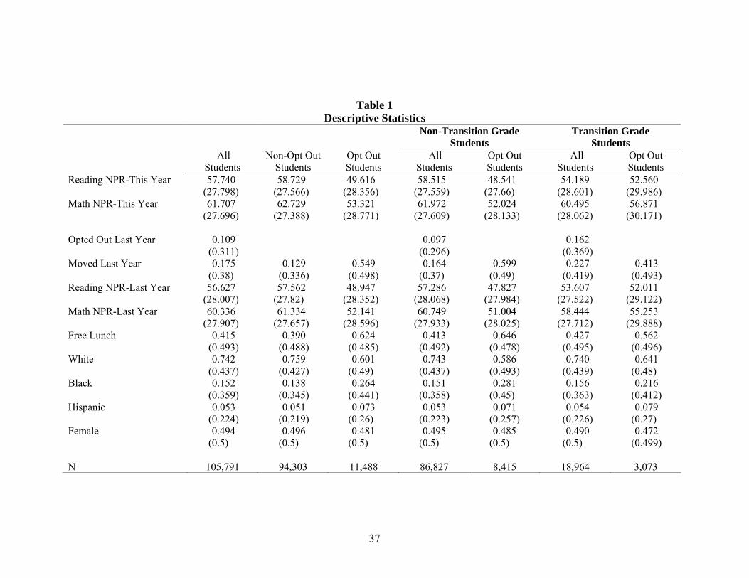
Table 1 provides the descriptive statistics for the entire sample as well as sub-

samples based on grade level and opt-out status. The average PCS student scores slightly

above the national median in both reading and math. Approximately 11 percent of all

students opted out of their default schools and the opt-out rate is significantly higher for

transition-grade students. The racial distribution in the sample is very similar to the racial

distribution of the general population in the U.S. with the exception of Hispanics, who

are underrepresented in the sample.

There are substantial differences between the students who opt out of their default

schools (opt out students) and those who stay (non-opt out students) in terms of their

observed characteristics. Opt out students perform significantly worse on standardized

tests during the year prior to opting out, are more likely to be free-lunch students,

African-American and are more likely to have changed residences during the summer

before opting out. It is also worth noting the differences between the students who opt out

after the transition grade and those who opt out after a non-transition grade. Transition-

17 Pinellas County Schools is divided into approximately 900 transportation grids. For each student residing within the boundaries of a given grid, transportation is provided to only one public school at each school level. 18 Using the transportation grids, I find the attendance zone for a given public school at each school year by aggregating the grids in which the majority of students attend that public school during that year.

12

grade opt-out students have significantly higher prior achievement levels than non-

transition grade opt-out students and are more similar to non-opt out students at the same

grade level. The average non-transition grade opt out student is ranked roughly 4

percentiles lower than the average transition-grade opt-out student in both reading and

math tests during the previous year.

3. Impact of Open Enrollment on School Choice

3.1. Incidence of opting out

Reducing the costs associated with opting out of the default public school, open

enrollment programs allow students, who could not otherwise afford to exercise other

traditional public schooling options, to opt out. Therefore, one would expect an increase

in the rate of students who opt out of their default schools with the introduction of this

policy. Figure 1 presents the opt-out rates in PCS between 2001 and 2005 for the entire

sample as well as for transition grade and non-transition grade students.

The implementation of open enrollment at the end of 2002-2003 school year in

PCS had a significant impact on the opt-out rate for the entire sample in the years

following the policy adoption. The opt-out rate more than doubled in the first year after

the policy change, from 7 percent to 18 percent, and then declined slightly in the

following year. Comparing the two sub-groups, the results indicate that the transition

graders reacted more to the increasing school choice. With the enactment of the choice

program, the rate of opting out among transition graders quadrupled from 8 percent to 33

percent in the first year and further increased to 38 percent in the second year. The non-

13

transition grade opt-out rate, on the other hand, increased from 7 percent to 16 percent

during the first year and then declined 12 percent in the following year.19

3.2. Composition of the opt-out students

During both pre-policy and post-policy periods, each student will opt out of her

default public school if the discontent or the ‘anticipated’ displeasure with the default

school overwhelms the cost of opting out. Therefore, by lowering the cost, open

enrollment programs will induce ‘less-discontented’ or ‘less-motivated to opt-out’

students to opt-out. If those who opted-out before the enactment of open enrollment were

mainly the ‘bad apples’ with the lowest achievement levels in their original schools, then

open enrollment will induce students with relatively higher achievement levels to

exercise other public alternatives. On the other hand, if those who opted out pre-policy

were mainly the ‘high-achievers’ in their ‘sending’ schools, who were dissatisfied with

the quality of their default public school, open enrollment will result in relatively low

achievers to opt out.

Figures 4.1 and 4.2 present the Kernel density estimates for the prior achievement

percentiles of the opt-out students in the sending school compared to their peers at the

same grade level. During the pre-policy period, for the non-transition graders, the opt-out

students were mainly the lowest achievers in their ‘sending’ schools: approximately 25

percent of the non-transition grade opt-out students were in the lowest two deciles of the

grade-level achievement distribution at their sending schools. As predicted, increasing

19 There are two possible explanations to this decline. First, the significant increase in the opt-out rates after the 5th grade during the first year after the policy change might have resulted in a decline in the rate of students who opt out at the end of the 6th grade during the second year. Furthermore, since non-transition grade students were not required to submit their public school preferences after the first year of policy adoption, the increasing cost of opting out might have altered the school choice behavior of the ‘marginally-displeased’ parent.

14

choice attracted relatively higher-achievers to opt out and this rate declined to 15 percent

with the enactment of open enrollment.

On the contrary, those who opted-out of their default middle schools at the end of

the 5th grade during the pre-policy period were mainly the highest achievers at their

sending schools: approximately 31 percent of the transition grade opt out students were in

the highest two deciles of the grade-level achievement distribution at their sending

schools in both reading and math. The open enrollment program induced relatively lower

achievers to opt-out for this subgroup: only 18 percent of the post-policy opt-out students

were in the highest two deciles in the post-policy period20. In each case, the Wilcoxon

test for equality of pre-policy and post-policy achievement distributions provides further

evidence that the policy change altered the composition of opting out students

significantly.

4. Opting Out and Student Test Scores

The extent to which exercising the school choice provided by open enrollment

translates into higher student achievement depends on households’ primary motives

behind opting out and households’ ability to exercise higher-quality schooling options. If

households are more achievement-oriented in their public school choices, then open

enrollment will result in more students attending higher-quality schools or schools that

are better matches to their needs, leading to improvements in the achievement levels of

the opt-out students due to the increased school input and possibly increased motivation.

Moreover, the increased competition for students among public schools might lead to an

improvement in the overall quality of public education, increasing the school input for all

20 I repeat the same analysis using the previous year test scores (absolute achievement at the sending school rather than relative) for the opt-out students; however, the conclusion remains unchanged.

15

students. However, these predicted effects of open enrollment will be limited if frictions

such as public school capacity constraints restrict students’ ability to exercise higher

quality public schooling options. On the other hand, if households make their public

school choices primarily based on non-academic characteristics of schools such as

proximity, then students should experience no increase in the school input and

consequently no benefit from opting out.

4.1. Where do students opt out?

In order to identify the mechanisms thru which exercising this form of school

choice impacts student test scores, it is essential to examine the extent to which students

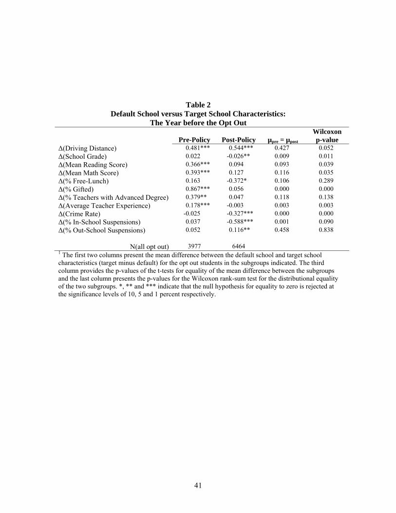
were able to exercise higher-quality public schooling options. For this purpose, I compare

the default school and target school of the opt-out students along three major dimensions:

non-academic characteristics, ‘direct’ measures of school quality and ‘indirect’ measures

of school quality. ‘Driving distance to the student’s residence’ is the main component of

the non-academic characteristics. For ‘direct’ academic measures, I use the Florida A+

program school grade21, the average math and reading scores, average teacher

experience, % teachers with advanced degrees, which serve as a proxy for the

instructional quality, % free-lunch students and % gifted students, which measure the

peer quality, in the school year prior to the opt-out. ‘Indirect’ academic measures include

the crime rates, % in-school suspensions and % out-school suspensions during the school

year prior to the opt-out.

21 Since 1999, as part of Florida’s A+ plan, public schools have been annually evaluated based on their students’ performance in the statewide Florida Comprehensive Assessment Test (FCAT). The grade of each school, which may range between A and F, depends on (1) overall performance of their students on FCAT; (2) the percentage of eligible students who take the test and (3) whether or not students have made annual learning gains in reading and math, with particular attention to the reading and math scores of the lowest 25% of students in the school.

16

The first column of Table 2 presents the pre-policy mean of the difference

between the default school and target school characteristics (target minus default) for the

opt-out students. The results suggest that the average student opts out to a public school

0.5 miles farther away from her residence. Prior to open enrollment, the average opt-out

student attended a school with slightly higher average test scores (0.4 percentiles in both

reading and math), % of advanced degree teachers (0.32%), higher average teacher

experience (0.18 years), higher % of gifted students (0.87%) during the year preceding to

the opt-out. However, during this period, the average opt-out student did not experience

any statistically significant changes in terms of indirect academic measures.

On the other hand, during the post-policy period, the gains experienced by the

opt-out students are only statistically different than zero for two of the seven direct

academic measures. In contrary to the pre-policy period, the average opt-out student in

the post-policy period opted out to ‘safer’ public schools: on average, the target school

had 0.3 less crimes per 100 students, 0.6% less in-school suspensions and 0.1% less out-

school suspensions. However, the t-test results for the equality of pre-policy means and

post-policy means, along with the Wilcoxon test results presented in the third and fourth

columns of Table 2 respectively, indicate that the gains experienced by the opt-out

students are not statistically different between pre-policy and post-policy periods for the

majority of the school characteristics.

Overall, despite the fact that some of the differences in school quality between the

target and default schools are statistically different from zero at conventional levels, none

is economically significant. For instance, the average opt-out student in the sample

attends a school with only 0.07 years of higher average teacher experience, whereas the

17

average teacher experience for the public schools in the sample is 13 years. Therefore,

although students travel more in order to opt out of their default public schools, their

target schools are very similar to their default schools along observed characteristics.

4.2. OLS Results

In order to quantify the relationship between opting out and student achievement,

I first estimate the following equation using OLS:

itatsgGtittiitit XXyOy εγηλβββββ ++++++++= − 541,310 (1)

where represents the end-of-year test score of student i during year t standardized to

mean zero and unit variance; is an indicator for students who opted out of their

default public schools at the beginning of the school year; represents the previous

year test score of student i in the same subject to control for the intrinsic ability of the

student; denotes the vector of students characteristics such as race, gender, an

indicator for whether the student changed residences during the summer before the school

year and free-lunch status, which serves as a proxy for the socio-economic status of the

student;

ity

itO

1, −tiy

itX

gλ is a grade fixed-effect to control for the test score differences between

grades; and tsη is a default school-year fixed-effect to control for the time-varying school

input at the default school22. In order to control for the time-invariant and time-varying

neighborhood inputs, I use attendance zone fixed-effects ( aγ ) and the average student

characteristics at the transportation grid level for each year ( GtX ) respectively.

22 Using default school-year fixed effects, I intend to compare the opt-out students to their similar peers who stayed behind. If a student opts out to a higher quality school, the impact of the relative increase in her school input compared to her peers at the default school will show in the coefficient of the ‘opt-out' variable.

18

Table 3 provides the OLS estimates of 1β , the parameter of interest, for the entire

sample as well as the transition graders and non-transition graders. The results suggest

that there is no statistically significant impact of opting out on test scores for the entire

sample. The results further suggest that the impact of opting out is quite different for the

two subgroups of interest. Transition-grade students who opt out of their default schools

perform slightly better than similar students who stay behind in reading whereas the

opposite is true for non-transition graders: opting-out, on average, is associated with

declines of 2 and 3 percent of the standard deviation in reading and math respectively for

non-transition graders.

4.3. IV Results

The major problem with the OLS analysis in this context is the inability to control

for all differences between those who opt-out and those who stay behind including

‘intrinsic motivation to excel’, which is positively correlated with student achievement. If

those who travel are more academically-motivated than similar students who stay behind,

OLS results will overestimate the true impact of opting out on student test scores.

Furthermore, the OLS results will provide overestimates/underestimates of the true

impact of opting out if those who stay behind suffer/benefit from the departure of their

peers who opted out. However, this source of bias should be rather limited in the sample

due to the relatively low opt-out rates (0.11 for the entire sample).

In order to deal with this selection issue, I instrument for opting out using the sum

of the reciprocal driving distances to the ‘relevant public alternatives’. Specifically, the

instrument is defined as follows:

19

( )

( )⎪⎪⎩

⎪⎪⎨

⎧

≤

>

=∑

∑

∈

∈

2003,

1

2003,

1

Proximityit

tifsrd

tifsrd

tij

areatij

Ss jit

Ss jit

where d(rit, sj) is the driving distance between the residence of student i at time t (rit) and

school sj, denotes the set of public schools at the school level of student i at time t

other than the ‘default’ public school within the attendance area of student i at time t, and

denotes the set of public schools at the school level of student i at time t other than the

‘default’ public school in the entire district

areaitS

itS

23. Compared to the previously used measures

of proximity, this instrument captures the student’s access to public alternatives better,

since it does not confine choice to the ‘closest alternative’, while realizing the negative

relationship between the distance to the public alternative and the relevance of that

alternative for the household.

Proximity has been shown to be a significant determinant of households’ public

school choice24. This is especially true in PCS where ‘proximity to the public school’ is

used as a priority category to determine the public school assignments after the enactment

of open enrollment. In the sample, for 77 percent of the students who stayed, the default

public school is one of the three closest public schools whereas this number is 59 percent

among the traveling students.

23 In order to construct the instrument, I first find the driving distances from the residential address of each student to each public school at the student’s school level in the district using Mapquest©. This requires the calculation of driving distances between roughly 32,000 residential addresses for elementary school students and 74 elementary public schools (2,350,000 distances), and 40,000 residential addresses for middle school students and 21 middle schools (840,000 distances). By identifying and excluding the default school for each student, I then calculate sum of the reciprocal distances to the relevant public alternatives for each student. 24 See Hastings, Kane and Staiger (2008).

20

The validity of the instrument relies on the condition that households, which are

similar in observable characteristics and reside within the attendance zone of a given

public school, are not stratified along any unobserved dimension such as the taste for

education, which would simultaneously impact the probability of opting out and student

achievement, with respect to the proximity to the relevant public alternatives25. Naturally,

households’ residential choices are not random; most households make their residential

choices with school characteristics as one of the determinants. However, provided that a

household chooses to reside within the boundaries of an attendance zone, it is unlikely

that the proximity to the relevant alternatives will play a significant role in the

household’s residential choice within that zone26.

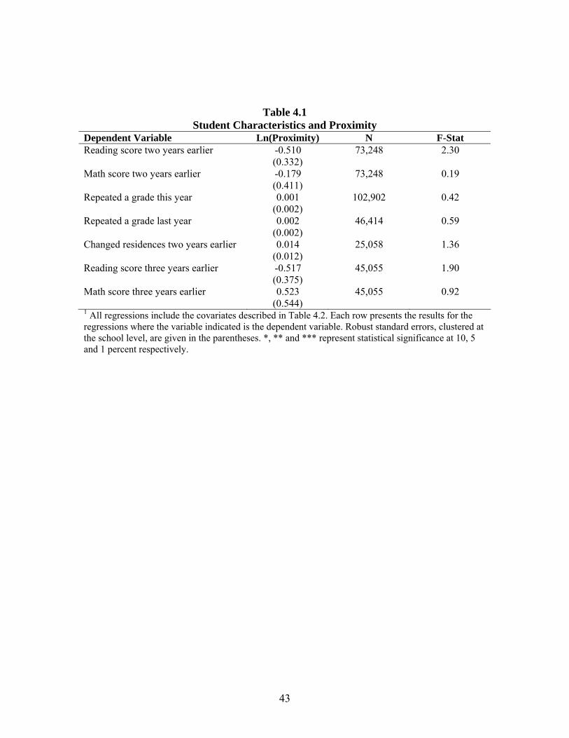
Table 4.1 provides further evidence on the validity of the instrument. Each row in

the table presents the estimated impact of the proximity measure on various

‘uncontrolled’ student characteristics in equation (1), controlling for the same covariates

in the original model with the addition of the distance to the default public school. The F-

stats presented in the third column suggest that the instrument has no statistically

significant impact on any of these ‘uncontrolled’ characteristics conditional on the

covariates listed in equation (1).

One must realize the two important limitations of this study while interpreting the

IV results. First, this study ignores the possibility that, in the absence of choice, students

could opt out of their assigned public schools by relocating or exercise private or non- 25 This follows, since I control for residential location via attendance-zone fixed effects in the model. 26 It is worth emphasizing the significance of residential location controls for the analysis. The instrument is clearly correlated with the school density in the area where the household resides. If those who reside in urban areas with relatively high student population and school density differ on unobservable achievement-related characteristics than those who chose to reside in relatively rural areas, then the instrument will impact student achievement in ways other than its impact on opting out. However, restricting the variation in the instrument to within attendance zones, which have an average area of three square miles, I overcome this issue.

21

traditional public schooling options such as charter schools and countywide fundamental

schools27. This limitation makes it hard to compare the well-being of the opt-out students

in the presence and the absence of open enrollment. Furthermore, if the increasing

competition between public schools, which is expected to impact the low-performing

public schools disproportionately, leads to an improvement in the overall quality of

public education, the IV results will provide underestimates of the true impact of opting

out on test scores.28

The second row of Table 4.2 presents the first-stage results of the IV regression

for the entire sample, non-transition grade students and the transition grade students. In

addition to the covariates defined earlier in equation (1), I also control for the driving

distance to the ‘default’ school, which is expected to have a positive impact on opting

out. The first-stage results indicate exceptionally strong correlation between proximity to

alternative schools and the probability of opting out of the default public school. The

students with more nearby public school alternatives, as determined by the proximity

measure, are more likely to exercise other public schooling options and the relationship is

extremely statistically significant for the entire sample as well as the two subgroups, as

indicated by the F-tests of significance of the excluded instrument for each regression.

The second-stage results, which are reported in the first row of Table 4, confirm

the earlier prediction on the direction of the bias in the OLS estimates. For the entire

sample and the non-transition graders, IV results suggest a significantly stronger negative

27 Roughly 15% of the entire K-12 student body in Pinellas County attend private schools, whereas the percentage attending non-traditional public options is significantly lower (0.5% in charter schools and 4% in countywide fundamental public schools). 28 This statement is true assuming that those who opt out of their default public schools attend higher-quality public alternatives. However, the earlier results indicate that this has not been the case in Pinellas County.

22

impact of opting out on reading test scores than the OLS estimates. The average opt-out

student is ranked roughly one-fourth of the standard deviation lower in reading test scores

than a similar student who stays behind. This detrimental impact of traveling on reading

scores is slightly higher for non-transition graders. On the other hand, there is neither any

statistically significant benefit/loss associated with opting out on math scores nor for

those who opted out of their default middle schools at the end of the 5th grade.

Table 5 compares the pre-policy and post-policy impacts of opting out on student

test scores. The post-policy opt-out is associated with a significantly higher reduction in

reading test scores compared to pre-policy: the pre-policy average opt-out student is

ranked roughly one-fifth of the standard deviation lower in reading compared to the one-

third of the standard deviation reduction after open enrollment. One possible explanation

to this puzzling result is the change in the composition of the opt-out students with the

enactment of open enrollment. The ‘new’ opt-out students are more mediocre and

possibly less-motivated to excel than their pre-policy counterparts. Another plausible

explanation is that it takes time for parents to comprehend the new system and make

‘good’ choices for their children. This is especially true in PCS, where a relatively

complicated mechanism, commonly known as the ‘Boston’ mechanism, is used to

determine the public school assignments. Not being strategy-proof, the Boston

mechanism makes it even harder for parents to submit the ‘optimal’ list of public school

preferences by providing some parents incentives to misreport their preferences29.

29 See Abdulkadiroglu and Sonmez (2003) for more detailed information about the Boston mechanism.

23

4.4. Disentangling the reasons underlying the detrimental impact

4.4.1. Change in school quality

There are several competing mechanisms through which opting opt might impact

student test scores. If those who opt-out of their default public schools are able to

exercise higher-quality schooling options, all else constant, opting out is expected to lead

to an increase in the traveling student’s test scores.

In order to quantify the impact of changing school quality for the traveling

students on test scores, Table 6 presents the estimated impact of opting out on reading

scores with and without controls for the change in the school quality experienced by

those who opt out. The first column replicates the first column of Table 4.2, whereas the

second, third and the fourth columns introduce attended school characteristics30, attended

school fixed-effects and attended school-year fixed effects to the model respectively.

Since our baseline model includes default school-year fixed-effects, the difference in the

estimated coefficients of the opt-out variable between the first specification and the

others should provide the impact of changing school quality caused by the opt-out on

reading scores. The estimated impact of opting out remains relatively stable across

specifications confirming the earlier finding that students, on average, opt out to ‘similar’

schools and hence do not experience significant improvements in their school inputs.

4.4.2. Outsider effect

The second mechanism through which opting out might affect student

achievement is changing intrinsic motivation of the traveling students. If being an

‘outsider’ at the new school leads to a decline in the intrinsic motivation of the student,

30 Attended school characteristics include the school grade in the previous year, average test scores in the previous year, average teacher experience, % teachers with advanced degrees, % gifted students, % free-lunch eligible students, crime rates and suspension rates.

24

then opting out might have a detrimental impact on test scores. If the outsider effect is

valid, then students who opt out of their default schools closer to the terminal grade of the

school level are expected to suffer more from doing so, since they will have less time and

incentives to become acquainted with the new environment. Furthermore, keeping the

proximity to the terminal grade of the school level constant, elementary school students

are expected to suffer more from non-transition grade opting out, since their new peers at

the target school are likely to have spent more time together, which makes it harder for

the traveling student to become an ‘insider’. Finally, if the intrinsic motivation of the

traveling students increases as they become more familiar to the new school, one might

expect the negative impact of opting out to vanish in the long run.

The IV results presented in Table 7 support the first prediction: those who opt out

of their default public schools one year before the terminal grade of the school level

experience significant declines in both reading (roughly one-fourth of the standard

deviation, yet marginally significant at conventional levels) and math (half of the

standard deviation) whereas opting-out of the default public school two years before the

terminal grade leads to a significant improvement (one-third of the standard deviation) in

the math scores of the traveling students.

Comparing the impact of non-transition grade opting out between elementary

school students and middle school students, the findings presented in Table 8 provide

evidence supporting the second prediction. Non-transition grade opting out during

elementary school years is associated with significant declines in both reading (one third

of the standard deviation) and math (one fourth of the standard deviation), whereas there

25

is no statistically significant impact of non-transition grade opting out on test scores

during middle school.

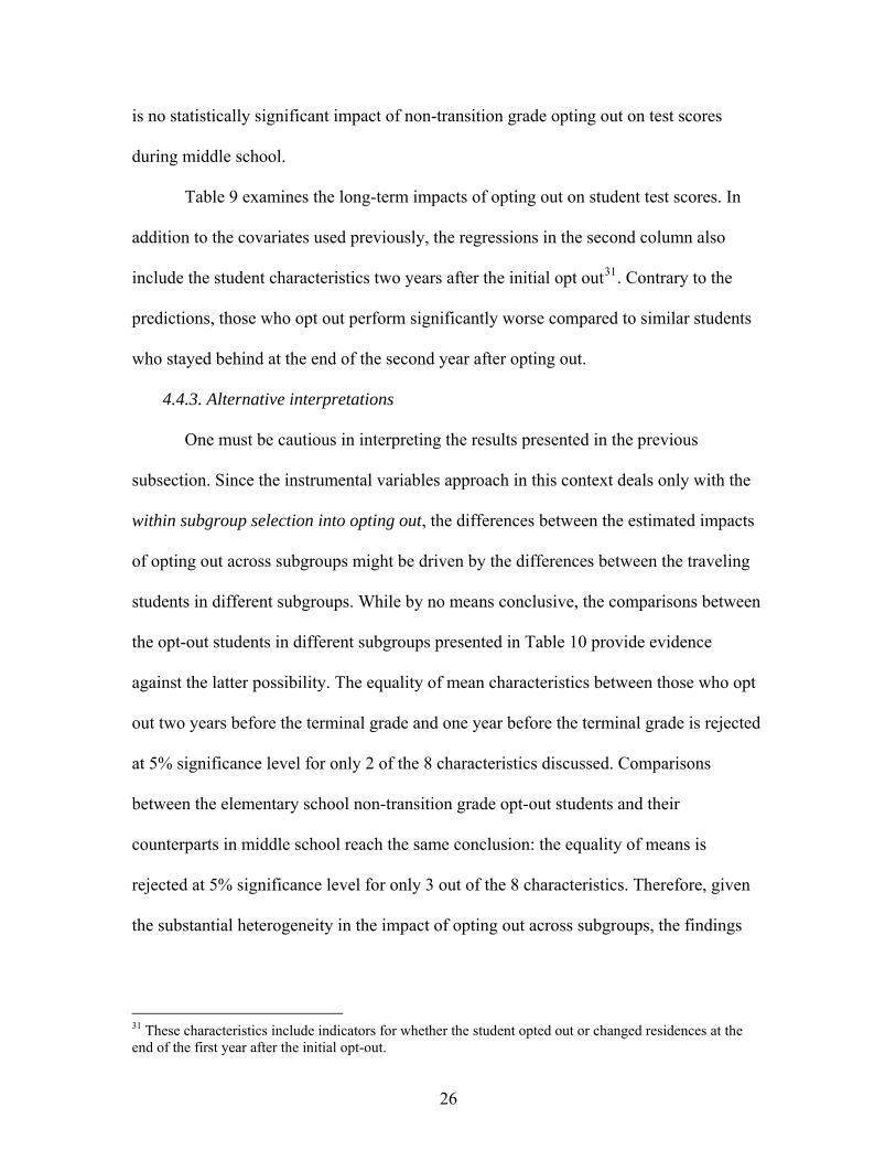
Table 9 examines the long-term impacts of opting out on student test scores. In

addition to the covariates used previously, the regressions in the second column also

include the student characteristics two years after the initial opt out31. Contrary to the

predictions, those who opt out perform significantly worse compared to similar students

who stayed behind at the end of the second year after opting out.

4.4.3. Alternative interpretations

One must be cautious in interpreting the results presented in the previous

subsection. Since the instrumental variables approach in this context deals only with the

within subgroup selection into opting out, the differences between the estimated impacts

of opting out across subgroups might be driven by the differences between the traveling

students in different subgroups. While by no means conclusive, the comparisons between

the opt-out students in different subgroups presented in Table 10 provide evidence

against the latter possibility. The equality of mean characteristics between those who opt

out two years before the terminal grade and one year before the terminal grade is rejected

at 5% significance level for only 2 of the 8 characteristics discussed. Comparisons

between the elementary school non-transition grade opt-out students and their

counterparts in middle school reach the same conclusion: the equality of means is

rejected at 5% significance level for only 3 out of the 8 characteristics. Therefore, given

the substantial heterogeneity in the impact of opting out across subgroups, the findings

31 These characteristics include indicators for whether the student opted out or changed residences at the end of the first year after the initial opt-out.

26

presented in Tables 7 and 8 can be regarded as evidence supporting the outsider effect

discussed in the previous subsection.

4.5. Impact of opting out- disadvantaged students

One of the main objectives of school choice reforms such as open enrollment is to

enable the ‘disadvantaged’ students such as those from low-SES families, who cannot

otherwise afford better schooling options, to attend higher-quality public schools. If the

‘disadvantaged’ students are more likely to opt out to higher-quality public schools

compared to their default public schools, they are expected to benefit more or suffer less

from opting out, since they will experience higher gains in school quality relative to the

‘advantaged’ students.

I define ‘disadvantaged’ students in two ways: with respect to the poverty and the

performance levels of their default public schools. High poverty schools are defined as

schools in which the majority of the students are free-lunch eligible in at least three of the

five years between 2001 and 2005, whereas the opposite indicates low poverty. High

performing schools are defined as having received a grade of ‘A’ in at least three years

during this time period, whereas the opposite indicates low performance.

Table 11 presents comparisons between the gains in school quality experienced

by the two subgroups. The results indicate that the ‘disadvantaged’ students experience

significantly higher gains in school quality compared to their ‘advantaged’ counterparts

regardless of the definition of ‘disadvantaged’.32

The IV estimates presented in the first set of rows of Table 12 partially verify the

expectations: opting out is associated with a significant decline in reading test scores for

32 For instance, those who opt-out of their low performing default schools attend public schools with 4% less free-lunch eligible students, whereas those who opt-out of their high performing default schools experience an increase of 5% in the percentage of free-lunch eligible students.

27

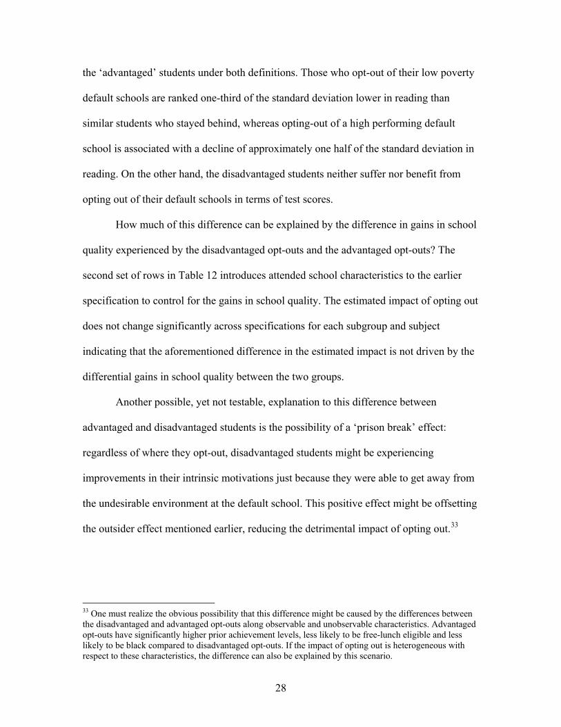
the ‘advantaged’ students under both definitions. Those who opt-out of their low poverty

default schools are ranked one-third of the standard deviation lower in reading than

similar students who stayed behind, whereas opting-out of a high performing default

school is associated with a decline of approximately one half of the standard deviation in

reading. On the other hand, the disadvantaged students neither suffer nor benefit from

opting out of their default schools in terms of test scores.

How much of this difference can be explained by the difference in gains in school

quality experienced by the disadvantaged opt-outs and the advantaged opt-outs? The

second set of rows in Table 12 introduces attended school characteristics to the earlier

specification to control for the gains in school quality. The estimated impact of opting out

does not change significantly across specifications for each subgroup and subject

indicating that the aforementioned difference in the estimated impact is not driven by the

differential gains in school quality between the two groups.

Another possible, yet not testable, explanation to this difference between

advantaged and disadvantaged students is the possibility of a ‘prison break’ effect:

regardless of where they opt-out, disadvantaged students might be experiencing

improvements in their intrinsic motivations just because they were able to get away from

the undesirable environment at the default school. This positive effect might be offsetting

the outsider effect mentioned earlier, reducing the detrimental impact of opting out.33

33 One must realize the obvious possibility that this difference might be caused by the differences between the disadvantaged and advantaged opt-outs along observable and unobservable characteristics. Advantaged opt-outs have significantly higher prior achievement levels, less likely to be free-lunch eligible and less likely to be black compared to disadvantaged opt-outs. If the impact of opting out is heterogeneous with respect to these characteristics, the difference can also be explained by this scenario.

28

4.6. Falsification Test

So far, I have attributed households’ changing school choice behavior to the

introduction of open enrollment in Pinellas County Schools. However, it is quite possible

that these behavioral changes had taken place due to some idiosyncratic factors or other

concurring educational reforms other than open enrollment. In contrary to the previous

literature, the existence of pre-policy data enables me to test this possibility. For this

purpose, I propose the following falsification exercise.

Consider an elementary school student residing in ‘attendance-area A’. Prior to

the adoption of open enrollment, the cost of opting out to a public school in attendance

area-A for the student should be similar to opting out to any public school in another

attendance area given that the two schools are equidistant to the student’s residence.

Therefore, pre-policy, proximity to the alternative public schools in attendance area-A

(policy alternatives) as well as the proximity to the alternative public schools in other

post-policy attendance areas (non-policy alternatives) should have explanatory power on

the student’s opt-out probability.

On the other hand, by allowing the student only to choose among public schools

in attendance area-A, the new ‘choice plan’ in PCS effectively decreased the relative cost

of attending area-A elementary schools for the student. This implies that, post-policy, the

relevant alternatives are only the ones within the attendance area of the student.

Therefore, after the policy change, only the proximity to the policy alternatives should

have explanatory power on the student’s opt-out probability.

Table 13 presents the linear probability model estimates where the outcome of

interest is the likelihood of opting-out. In addition to the two proximity measures, the

29

model includes the covariates described in Table 4.2. As predicted, during the pre-policy

period, both proximity measures have statistically significant impacts on the likelihood of

opting out. However, after the policy change, only the proximity to policy alternatives

has significant impact on households’ public school choice. These results provide

evidence that the households’ changing school choice behavior can be regarded as a

reaction to the adoption of open enrollment.

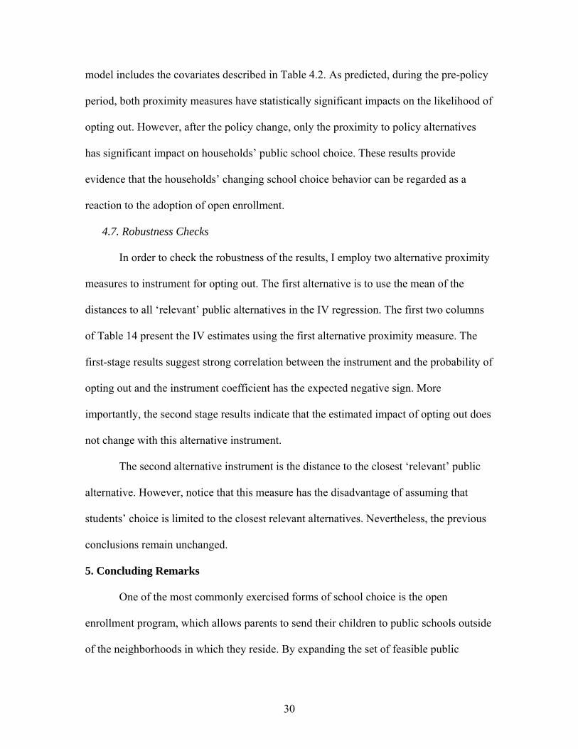
4.7. Robustness Checks

In order to check the robustness of the results, I employ two alternative proximity

measures to instrument for opting out. The first alternative is to use the mean of the

distances to all ‘relevant’ public alternatives in the IV regression. The first two columns

of Table 14 present the IV estimates using the first alternative proximity measure. The

first-stage results suggest strong correlation between the instrument and the probability of

opting out and the instrument coefficient has the expected negative sign. More

importantly, the second stage results indicate that the estimated impact of opting out does

not change with this alternative instrument.

The second alternative instrument is the distance to the closest ‘relevant’ public

alternative. However, notice that this measure has the disadvantage of assuming that

students’ choice is limited to the closest relevant alternatives. Nevertheless, the previous

conclusions remain unchanged.

5. Concluding Remarks

One of the most commonly exercised forms of school choice is the open

enrollment program, which allows parents to send their children to public schools outside

of the neighborhoods in which they reside. By expanding the set of feasible public

30

schools for households, such programs are predicted to impact households’ public school

choice as well as student achievement.

Using the recent school-choice policy change in Pinellas County Schools, I first

examine the impact of open enrollment on households’ public school choice behavior. I

find significant changes in the frequency of opting out of the default school and attending

another traditional public school, as well as the composition of those who exercise this

choice with the adoption of the open enrollment policy.

I then attempt to quantify the causal relationship between exercising this form of

school choice and student test scores. Using proximity to relevant ‘traditional’ public

alternatives as an instrument for opting out, the results indicate no significant benefit of

opting out and that those who opt out often perform significantly worse on standardized

tests than similar students who stay behind.

Furthermore, I find that the impact of opting out is significantly heterogeneous

with respect to the grade of opting out. The findings suggest that those who opt out

during elementary school years suffer significantly both in terms of reading and math

scores, whereas there is no statistically significant impact on middle school students.

Furthermore, those who opt out two years before the terminal grade of the school level

significantly benefit in terms of their math scores whereas opting out one year prior to the

terminal grade is associated with a significant decline in both reading and math test

scores. Finally, the results indicate that the negative effect of opting out is non-existent

for ‘disadvantaged’ students, who typically constitute the proposed target of school

choice reforms. Such detrimental effects seem to persist at the end of the second year

after the initial opt out.

31

An important policy implication of the findings presented in this study is that

open enrollment programs fail to improve the achievement levels of those who exercise

this form of choice. One reason underlying this conclusion is the ‘highly constrained’

choice environment provided by such programs, which does not enable students to

exercise higher quality schooling options. The results indicate that those who opt out of

their default public schools, on average, attend ‘similar’ schools along various measures

of school quality. Along with the negative effect of opting out on the intrinsic motivation

of the students due to being an outsider at the new school, lack of gains in school quality

might explain the detrimental impact of opting out.

32

References

Abdulkadiroglu, Atila, and Tayfun Sonmez. 2003. “School Choice: A Mechanism Design

Approach.” American Economic Review 93(3): 729-747.

Cullen, Julie Berry, Brian A. Jacob, and Steven D. Levitt, 2005. “The Impact of School

Choice on Student Outcomes: An Analysis of the Chicago Public Schools.”

Journal of Public Economics 89: 729 – 760.

Cullen, Julie Berry, Brian A. Jacob, and Steven D. Levitt, 2006. “The Effect of School

Choice on Participants: Evidence from Randomized Lotteries.” Econometrica

74(5): 1191 – 1230.

Cullen, Julie Berry, and Brian A. Jacob. Forthcoming. “Is Gaining Access to a Selective

Elementary School Gaining Ground? Evidence from Randomized Lotteries.” In

An Economics Perspective on the Problems of Disadvantaged Youth, edited by

Jonathan Gruber. Chicago, IL: University of Chicago Press.

Education Commission of the States. 2005. State Notes: Open Enrollment: 50-State

Report.

Fiske, Edward B., and Helen Ladd. 2000. When Schools Compete: A Cautionary Tale.

Washington, D.C.: Brookings Institution Press.

Hastings, Justine S. and Jeffrey M. Weinstein. Forthcoming. “Information, School Choice

and Academic Achievement: Evidence from Two Experiments.” Quarterly Journal of

Economics.

Hastings, Justine S., Thomas Kane, and Douglas Staiger. 2008. “Heterogeneous

Preferences and the Efficacy of Public School Choice.” National Bureau of

Economic Research Paper Working Papers No. 12145 and No. 11805 combined.

33

National Center for Education Statistics. 2006. The Condition of Education 2006.

Organization for Economic Cooperation and Development. 2008. Education at a Glance

2008.

Organization for Economic Cooperation and Development. 2003. Programme for

International Student Assessment 2003.

34

Figure 1.1 Post-Policy Elementary School

Attendance Areas in PCS

35

36

Figure 1.2 Post-Policy Middle School Attendance Areas in PCS

37

Table 1

Descriptive Statistics

Non-Transition Grade

Students Transition Grade

Students All

Students Non-Opt Out

Students Opt Out Students

All Students

Opt Out Students

All Students

Opt Out Students

Reading NPR-This Year 57.740 58.729 49.616 58.515 48.541 54.189 52.560 (27.798) (27.566) (28.356) (27.559) (27.66) (28.601) (29.986) Math NPR-This Year 61.707 62.729 53.321 61.972 52.024 60.495 56.871 (27.696) (27.388) (28.771) (27.609) (28.133) (28.062) (30.171) Opted Out Last Year 0.109 0.097 0.162 (0.311) (0.296) (0.369) Moved Last Year 0.175 0.129 0.549 0.164 0.599 0.227 0.413 (0.38) (0.336) (0.498) (0.37) (0.49) (0.419) (0.493) Reading NPR-Last Year 56.627 57.562 48.947 57.286 47.827 53.607 52.011 (28.007) (27.82) (28.352) (28.068) (27.984) (27.522) (29.122) Math NPR-Last Year 60.336 61.334 52.141 60.749 51.004 58.444 55.253 (27.907) (27.657) (28.596) (27.933) (28.025) (27.712) (29.888) Free Lunch 0.415 0.390 0.624 0.413 0.646 0.427 0.562 (0.493) (0.488) (0.485) (0.492) (0.478) (0.495) (0.496) White 0.742 0.759 0.601 0.743 0.586 0.740 0.641 (0.437) (0.427) (0.49) (0.437) (0.493) (0.439) (0.48) Black 0.152 0.138 0.264 0.151 0.281 0.156 0.216 (0.359) (0.345) (0.441) (0.358) (0.45) (0.363) (0.412) Hispanic 0.053 0.051 0.073 0.053 0.071 0.054 0.079 (0.224) (0.219) (0.26) (0.223) (0.257) (0.226) (0.27) Female 0.494 0.496 0.481 0.495 0.485 0.490 0.472 (0.5) (0.5) (0.5) (0.5) (0.5) (0.5) (0.499) N 105,791 94,303 11,488 86,827 8,415 18,964 3,073

Figure 2 Percentage of Opt Out Students

0%

5%

10%

15%

20%

25%

30%

35%

40%

2001 2002 2003 2004 2005

All StudentsTransition Grade StudentsNon-Transition Grade Students

38

Figure 3.1 Kernel Density Estimates: Achievement Percentile at the ‘Sending’ School

Non-Transition Grade Opt Out Students Reading

Wilcoxon Rank-Sum Test (H0: Pre-policy = Post-policy) p-value = 0.000

Math


1 Both densities were estimated with an Epanechnikov kernel function and halfwidth of 5 percentiles.

39

Figure 3.2 Kernel Density Estimates: Achievement Percentile at the ‘Sending’ School

Transition Grade Opt Out Students Reading


Math


1 Both densities were estimated with an Epanechnikov kernel function and halfwidth of 5 percentiles.

40

41

Table 2 Default School versus Target School Characteristics:

The Year before the Opt Out

Pre-Policy Post-Policy µpre = µpost

Wilcoxon p-value

Δ(Driving Distance) 0.481*** 0.544*** 0.427 0.052 Δ(School Grade) 0.022 -0.026** 0.009 0.011 Δ(Mean Reading Score) 0.366*** 0.094 0.093 0.039 Δ(Mean Math Score) 0.393*** 0.127 0.116 0.035 Δ(% Free-Lunch) 0.163 -0.372* 0.106 0.289 Δ(% Gifted) 0.867*** 0.056 0.000 0.000 Δ(% Teachers with Advanced Degree) 0.379** 0.047 0.118 0.138 Δ(Average Teacher Experience) 0.178*** -0.003 0.003 0.003 Δ(Crime Rate) -0.025 -0.327*** 0.000 0.000 Δ(% In-School Suspensions) 0.037 -0.588*** 0.001 0.090 Δ(% Out-School Suspensions) 0.052 0.116** 0.458 0.838

N(all opt out) 3977 6464 1 The first two columns present the mean difference between the default school and target school characteristics (target minus default) for the opt out students in the subgroups indicated. The third column provides the p-values of the t-tests for equality of the mean difference between the subgroups and the last column presents the p-values for the Wilcoxon rank-sum test for the distributional equality of the two subgroups. *, ** and *** indicate that the null hypothesis for equality to zero is rejected at the significance levels of 10, 5 and 1 percent respectively.

42

Table 3 The Impact of Opting Out on Test Scores

OLS Results All Students Non-Transition Grade Students Transition Grade Students Reading Math Reading Math Reading Math

Opt out -0.005 -0.017 -0.022** -0.026** 0.039** 0.021 (0.010) (0.012) (0.009) (0.012) (0.018) (0.019)

Adjusted-R2 0.66 0.68 0.66 0.68 0.67 0.67 N 104,830 104,830 85,893 85,893 18,937 18,937

1 For each regression, test scores are standardized to mean zero and unit variance within the subgroup. All regressions include individual student characteristics (previous year test score in the same subject, free-lunch status, race, gender), indicator for whether the student changed her residence during the summer before the opt out, grade fixed-effects, ‘default’ school fixed-effects, year fixed-effects, ‘default’ school-year fixed-effects, attendance zone fixed-effects and transportation grid characteristics. Robust standard errors, clustered at the school level, are given in the parentheses. *, ** and *** represent statistical significance at 10, 5 and 1 percent respectively.

43

Table 4.1

Student Characteristics and Proximity Dependent Variable Ln(Proximity) N F-Stat Reading score two years earlier -0.510 73,248 2.30 (0.332) Math score two years earlier -0.179 73,248 0.19 (0.411) Repeated a grade this year 0.001 102,902 0.42 (0.002) Repeated a grade last year 0.002 46,414 0.59 (0.002) Changed residences two years earlier 0.014 25,058 1.36 (0.012) Reading score three years earlier -0.517 45,055 1.90 (0.375) Math score three years earlier 0.523 45,055 0.92 (0.544) 1 All regressions include the covariates described in Table 4.2. Each row presents the results for the regressions where the variable indicated is the dependent variable. Robust standard errors, clustered at the school level, are given in the parentheses. *, ** and *** represent statistical significance at 10, 5 and 1 percent respectively.

44

Table 4.2 The Impact of Opting Out on Test Scores

IV Results All Students Non-Transition Grade Students Transition Grade Students Reading Math Reading Math Reading Math

Opt out -0.236*** -0.062 -0.250** -0.048 -0.056 -0.103 (0.089) (0.100) (0.115) (0.113) (0.129) (0.149)

First Stage Results

Ln(Proximity) 0.086*** 0.086*** 0.078*** 0.078*** 0.132*** 0.132***

(0.006) (0.006) (0.006) (0.006) (0.015) (0.015)

F-Stat (Excluded Instr.) 238.39 238.39 184.68 184.68 76.03 76.03 N 104,830 104,830 85,893 85,893 18,937 18,937

1 For each regression, test scores are standardized to mean zero and unit variance within the subgroup. In addition to the covariates described in Table 3, all regressions include the driving distance to the ‘default’ public school. Robust standard errors, clustered al the school level, are given in the parentheses. *, ** and *** represent statistical significance at 10, 5 and 1 percent respectively.


Pre-Policy versus Post-Policy IV Results

Pre-Policy Post-Policy Reading Math Reading Math

Opt out -0.197* -0.032 -0.312** -0.116 (0.106) (0.164) (0.149) (0.172)

First Stage Results

Ln(Proximity) 0.082*** 0.082*** 0.076*** 0.076***

(0.008) (0.008) (0.008) (0.008)

F-Stat (Excluded Instr.) 115.56 115.56 103.43 103.43 N 63,275 63,275 41,555 41,555

1 For each regression, test scores are standardized to mean zero and unit variance within the subgroup. All regressions include the covariates described in Table 4.2. Robust standard errors, clustered at the school level, are given in the parentheses. *, ** and *** represent statistical significance at 10, 5 and 1 percent respectively.

Table 6 The Impact of Opting Out on Reading Scores

Identifying the Impact of Changing School Quality IV Results

I II III IV Opt out -0.236*** -0.210*** -0.263*** -0.257***

(0.089) (0.086) (0.094) (0.093)

Default school-year FE YES YES YES YES Attended school character. NO YES NO NO Attended school FE NO NO YES NO Attended school-year FE NO NO NO YES

First Stage Results

Ln(Proximity) 0.086*** 0.083*** 0.074*** 0.074***

(0.006) (0.005) (0.005) (0.005)


1 For each regression, test scores are standardized to mean zero and unit variance within the subgroup. All regressions include the covariates described in Table 4.2. Attended school characteristics include the school grade in the previous year, average test scores in the previous year, average teacher experience, % teachers with advanced degrees, % gifted students, % free-lunch eligible students, crime rate and suspension rates. Robust standard errors, clustered at the school level, are given in the parentheses. *, ** and *** represent statistical significance at 10, 5 and 1 percent respectively.

45

Table 7

The Impact of Opting Out on Test Scores Elementary versus Middle School Non-Transition Graders

IV Results Elementary School Middle School Reading Math Reading Math

Opt out -0.323*** -0.241** -0.112 0.247 (0.135) (0.121) (0.194) (0.172)

First Stage Results

Ln(Proximity) 0.124*** 0.124*** 0.052*** 0.052***

(0.010) (0.010) (0.007) (0.007)

F-Stat (Excluded Instr.) 144 144 55.20 55.20 N 39,693 39,693 46,200 46,200



By Years after Opting Out IV Results

One Year After Opting Out Two Years After Opting Out Reading Math Reading Math

Opt out -0.236*** -0.062 -0.289** -0.037 (0.089) (0.100) (0.127) (0.143)

F-Stat (Excluded Instr.) 244.29 244.29 139.94 140.19

N 104,830 104,830 54,939 54,939 1 For each regression, test scores are standardized to mean zero and unit variance within the subgroup. The regressions reported in the first two columns include the same covariates in Table 4.2. In addition, the last two regressions include indicators for whether the student opted out or moved during the summer prior to the second year. Robust standard errors are given in the parentheses. *, ** and *** represent statistical significance at 10, 5 and 1 percent respectively.

46

Table 9

The Impact of Opting Out on Test Scores By Grade of Opt Out

IV Results Two Years Before Terminal

Grade One Year Before Terminal

Grade Reading Math Reading Math

Opt out -0.157 0.346*** -0.230* -0.535*** (0.161) (0.127) (0.134) (0.225)

First Stage Results

Ln(Proximity) 0.086*** 0.086*** 0.071*** 0.071***

(0.008) (0.008) (0.008) (0.008)



Table 10

Student Characteristics across Subgroups Opted out one

year before the terminal grade

Opted out two years before the terminal grade

Elementary school opt-out

Middle school opt-out

Reading NPR-Last Year 47.721 48.124 48.114 47.665 (0.445) (0.431) (0.397) (0.493) Math NPR-Last Year 50.747 51.456 50.562* 51.891 (0.457) (0.422) (0.397) (0.496) Free Lunch 0.622*** 0.670 0.691*** 0.583 (0.008) (0.007) (0.007) (0.008) White 0.595 0.581 0.576** 0.604 (0.008) (0.008) (0.007) (0.008) Black 0.279 0.278 0.287* 0.266 (0.007) (0.007) (0.007) (0.008) Hispanic 0.067 0.076 0.070 0.074 (0.004) (0.004) (0.004) (0.005) Female 0.487 0.481 0.471** 0.502 (0.008) (0.008) (0.007) (0.009) Moved Last Year 0.632*** 0.574 0.597 0.609 (0.008) (0.008) (0.007) (0.008) N 3,971 4,201 4,792 3,380 1 *, ** and *** indicate that the null hypothesis for equality of means across subgroups is rejected at the significance levels of 10, 5 and 1 percent respectively.

47

Table 11 Default School versus Target School Characteristics

The Year before the Opt Out

Low Poverty High

Poverty µlp = µhp

Wilcoxon p-value

Δ(School Grade) -0.166*** 0.156*** 0.000 0.000 Δ(Mean Reading Score) -1.364*** 1.819*** 0.000 0.000 Δ(Mean Math Score) -1.172*** 1.682*** 0.000 0.000 Δ(% Free-Lunch) 4.492*** -5.005*** 0.000 0.000 Δ(% Gifted) 0.520*** 0.204*** 0.017 0.000 Δ(% Teachers with Advanced Degree)

-1.241*** 1.642*** 0.000 0.000

Δ(Average Teacher Experience) -0.208*** 0.350*** 0.000 0.000

N 5317 5124 High

Performing Low

Performing µhp = µlp

Wilcoxon p-value

Δ(School Grade) -0.269*** 0.213*** 0.000 0.000 Δ(Mean Reading Score) -2.440*** 2.439*** 0.000 0.000 Δ(Mean Math Score) -2.333*** 2.405*** 0.000 0.000 Δ(% Free-Lunch) 4.638*** -4.252*** 0.000 0.000 Δ(% Gifted) -0.679*** 1.252*** 0.000 0.000 Δ(% Teachers with Advanced Degree)

-1.304*** 1.428*** 0.000 0.000

Δ(Average Teacher Experience) -0.676*** 0.696*** 0.000 0.000

N 4796 5645 1 The first two columns present the mean difference between the default school and target school characteristics (target minus default) for the opt out students in the subgroups indicated. The third column provides the p-values of the t-tests for equality of the mean difference between the subgroups and the last column presents the p-values for the Wilcoxon rank-sum test for the distributional equality of the two subgroups. *, ** and *** indicate that the null hypothesis for equality to zero is rejected at the significance levels of 10, 5 and 1 percent respectively.

48


Disadvantaged Students IV Results

I. Without Attended School Characteristics Low Poverty

Default School High Poverty

Default School Reading Math Reading Math

Opt out -0.338* -0.025 -0.111 -0.070 (0.182) (0.157) (0.104) (0.155)

F-Stat (Excluded Instr.) 88.74 88.74 136.89 136.42

N 65,498 65,498 38,643 38,643 High Performing

Default School Low Performing Default School

Reading Math Reading Math Opt out -0.452** 0.052 -0.048 -0.123

(0.194) (0.165) (0.115) (0.149)


II. With Attended School Characteristics Low Poverty

Default School High Poverty

Default School Reading Math Reading Math

Opt out -0.353* -0.011 -0.097 -0.059 (0.195) (0.176) (0.101) (0.148)

F-Stat (Excluded Instr.) 78.32 78.32 144 143.52

N 65,386 65,386 38,250 38,250 High Performing

Default School Low Performing Default School

Reading Math Reading Math Opt out -0.477** 0.076 -0.044 -0.127

(0.217) (0.182) (0.120) (0.157)


1 For each regression, test scores are standardized to mean zero and unit variance within the subgroup. All regressions include the covariates described in Table 4.2. High poverty school is defined as having the majority of the students free-lunch eligible in at least three of the five years between 2001 and 2005, whereas the opposite indicates low poverty. High performance school is defined as receiving a grade of A in at least three of the years between 2001 and 2005, whereas the opposite indicates low performing. Robust standard errors, clustered at the school level, are given in the parentheses. *, ** and *** represent statistical significance at 10, 5 and 1 percent respectively.

49

Table 13 Falsification Test

Linear Probability Model Estimates Dependent Variable: Opt Out

Pre-Policy Post-Policy

Ln(Proximity to ‘Policy’ Schools) 0.045*** 0.076*** (0.010) (0.015)

Ln(Proximity to ‘Non-policy’ Schools) 0.054*** 0.004 (0.022) (0.035) F-Stat (Policy Schools) 19.44 25.15

F-Stat (Non-Policy Schools) 6.04 0.01 N 63,275 41,555

1 For each regression, test scores are standardized to mean zero and unit variance within the subgroup. Both regressions include the covariates described in Table 4.2. Robust standard errors,clustered at the school level, are given in the parentheses. *, ** and *** represent statistical significance at 10, 5 and 1 percent respectively.


IV Results – Robustness Checks I II Reading Math Reading Math

Opt out -0.223** -0.101 -0.225** -0.089 (0.099) (0.100) (0.105) (0.121)

First Stage Results

Ln(Mean Distance) -0.125*** -0.125***

(0.009) (0.009) Ln(Distance-Closest Alt.) -0.030 -0.030

(0.002) (0.002)


1 For each regression, test scores are standardized to mean zero and unit variance within the subgroup. All regressions include the covariates described in Table 4. Robust standard errors, clustered at the school level, are given in the parentheses. *, ** and *** represent statistical significance at 10, 5 and 1 percent respectively.

50

the effects of open enrollment on school choice and

Documents