the effects of heterogeneous spatial networks in multi ... · the effects of heterogeneous spatial...
TRANSCRIPT

The Effects of Heterogeneous Spatial Networks in Multi-agent Parrondo’s Games
Junyong Shu, Keren Rui, Ye Ye*, Lu Wang and Nenggang Xie School of Mechanical Engineering, Anhui University of Technology, Ma’anshan, Anhui Province, 243002, China
*Corresponding author Abstract—In the multi-agent Parrondo’s games, if game A and game B both take certain network structures, then the heterogeneity of the network will produce impacts. By using the analytical approach based on the discrete Markov chain, we analyzed a one-dimensional case. Then, we deduced the transition probability matrix of game A under one dimensional line (homogeneous with game B) and a fully-connected network (heterogeneous with game B). Moreover, we gave the mathematical expectation of the randomized game A+B. The theoretical results showed that for the one-dimensional case the heterogeneity between game A and game B enlarges the parameter space of the strong paradox. Besides, we performed calculation simulations on two-dimensional networks. We used the following four networks for game A: a two-dimensional lattice (homogeneous with game B), random network, a scale-free network and a fully-connected network (the latter three networks are heterogeneous with game B). The simulation results showed that the gain and the strong paradox space both decrease with the increment of the degree of the heterogeneous, which shows that homogeneity between game A and game B is beneficial for two-dimensional networks.
Keywords-parrondo's paradox, parrondo’s games, complex networks, heterogeneity
I. INTRODUCTION
Parrondo’s paradox is an apparent paradox in game theory, and it is named after its creator Parrondo, a Spanish physicist [1]. The seminal papers on Parrondo’s paradox were published by Abbott and Harmer [2-3] in 1999. Moreover, Parrondo’s paradox has been developed into many different versions [4]. Generally, Parrondo’s games involve two games, A and B. Game B has some branches, some of which are favorable (that is the probability of winning is large) and others are unfavorable (that is the probability of losing is large).The design of the branches requires some forms of dependence. At present, according to the available Parrondo’s games, the dependent mechanisms mainly include three types, which are based on the individual capital, on the individual history of experience and on neighbors’ environment. According to the size of the participants, there mainly includes individual and group versions. Toral [8] proposed a space-dependent “cooperative Parrondo’s paradox” version. A remarkable difference is that there are i (i=2, …, N) players instead of only one player involved in the game. However, here the multi-agent version was not carried out. Game A remained unchanged as was defined in the original Parrondo’s games. Game B, which was based on the neighboring environment. Wang [11] presented a version of Parondox’s paradox played
in a population of agents where game A was the original game based on the flip of a suitably biased coin and game B was a 2×2 game played between a pair of agents selected randomly. In this version, game B showed the characteristics of the multi-agent game, that is, individuals had interactive roles between themselves. As the previous versions have focused on how to modify game B, Toral [12] proposed a modification of game A. There were N players involved in this version as well and there was interaction between individuals for game A. Game B remained unchanged as defined in the original Parrondo’s games or in the history-dependent version. In the version proposed by Xie [13], game A was the same as that in Toral [12] and game B was played based on the neighboring environment. Here, game A and game B produced the coupling effects spatially.
For game A in the multi-agent versions, individuals have a interactive relationship, which belongs to a zero-sum game from the view of the population level. There are two key points in the interactive relationship: 1) The interactive modes. They can be divided into competition and cooperation. In the version proposed by Toral [12], individuals used the cooperative mode. Wang [14] presented four kinds of interaction, which were competition, cooperation, harmony and PCRC, respectively. 2) The network carriers. The population has a certain spatial distribution or a spatial structure which will be abstracted into a certain topology network in the theoretical analysis. Individuals interact through networks. In the version proposed by Toral [12], the network carriers were the fully-connected network and a one-dimensional line. Xie [13] also used a one-dimensional line. Wang [14] and Ye [15-16] adopted a fully-connected network, random network and a BA scale-free network as their spatial carriers. Moreover, they obtained that different network structures and the heterogeneity have different effects on the multi-agent Parrondo’s games.
In the above studies of Toral [12], Wang [14] and Ye [15-16], game A belonged to the multi-agent version and they use the capital-dependent and history-dependent mechanisms for game B. If game B was based on the neighboring environment mechanism, then game A and game B had the coupling effects. There are many network structures for game A while there are only one dimensional line and a two-dimensional lattice for game B due to the structure limitation. Xie [13] analyzed the multi-agent Parrondo’s game under the homogeneous networks. However, there are no relevant studies at present when game A and game B have different network carriers. For such a case, the paper demonstrates the effects of the heterogeneity of
139 This is an open access article under the CC BY-NC license (http://creativecommons.org/licenses/by-nc/4.0/).
Copyright © 2017, the Authors. Published by Atlantis Press.
Advances in Intelligent Systems Research (AISR), volume 141International Conference on Applied Mathematics, Modelling and Statistics Application (AMMSA 2017)
networks through the theoretical and computer simulation analysis.
II. THE THEORETICAL ANALYSIS BASED ON A ONE-DIMENSIONAL LINE
A. Model
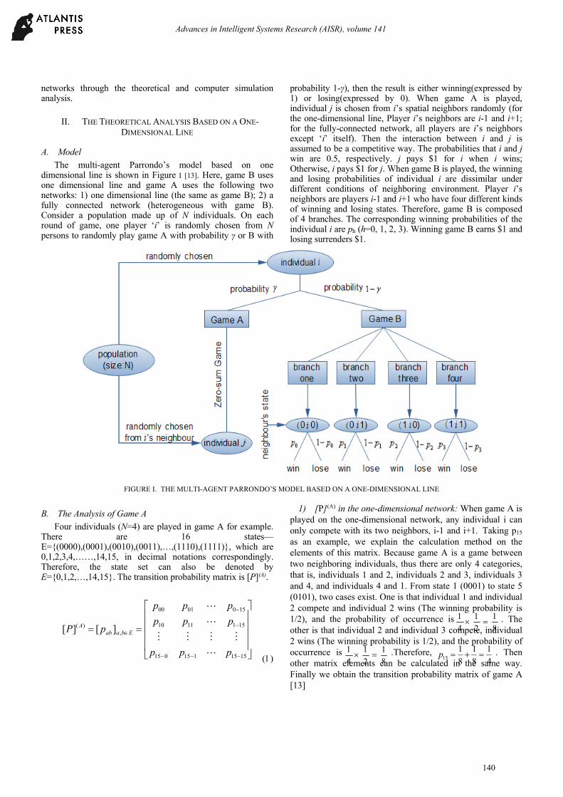
The multi-agent Parrondo’s model based on one dimensional line is shown in Figure I [13]. Here, game B uses one dimensional line and game A uses the following two networks: 1) one dimensional line (the same as game B); 2) a fully connected network (heterogeneous with game B). Consider a population made up of N individuals. On each round of game, one player ‘i’ is randomly chosen from N persons to randomly play game A with probability γ or B with
probability 1-γ), then the result is either winning(expressed by 1) or losing(expressed by 0). When game A is played, individual j is chosen from i’s spatial neighbors randomly (for the one-dimensional line, Player i’s neighbors are i-1 and i+1; for the fully-connected network, all players are i’s neighbors except ‘i’ itself). Then the interaction between i and j is assumed to be a competitive way. The probabilities that i and j win are 0.5, respectively. j pays $1 for i when i wins; Otherwise, i pays $1 for j. When game B is played, the winning and losing probabilities of individual i are dissimilar under different conditions of neighboring environment. Player i’s neighbors are players i-1 and i+1 who have four different kinds of winning and losing states. Therefore, game B is composed of 4 branches. The corresponding winning probabilities of the individual i are ph (h=0, 1, 2, 3). Winning game B earns $1 and losing surrenders $1.
FIGURE I. THE MULTI-AGENT PARRONDO’S MODEL BASED ON A ONE-DIMENSIONAL LINE
B. The Analysis of Game A
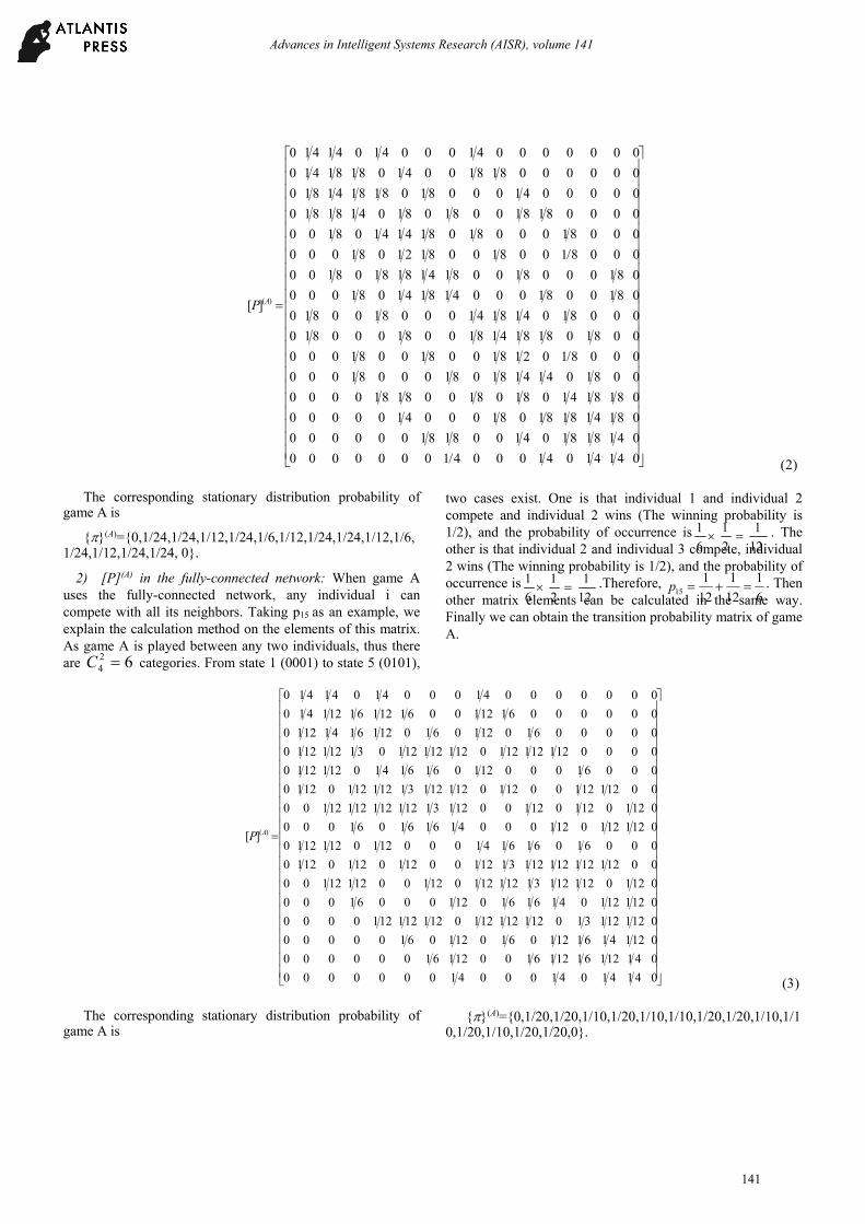
Four individuals (N=4) are played in game A for example. There are 16 states—E={(0000),(0001),(0010),(0011),…,(1110),(1111)}, which are 0,1,2,3,4,……,14,15, in decimal notations correspondingly. Therefore, the state set can also be denoted by E={0,1,2,…,14,15}. The transition probability matrix is [P](A).
1515115015
1511110
1500100
,)( ][][
ppp
ppp
ppp
pP EbaabA
1) [P](A) in the one-dimensional network: When game A is played on the one-dimensional network, any individual i can only compete with its two neighbors, i-1 and i+1. Taking p15 as an example, we explain the calculation method on the elements of this matrix. Because game A is a game between two neighboring individuals, thus there are only 4 categories, that is, individuals 1 and 2, individuals 2 and 3, individuals 3 and 4, and individuals 4 and 1. From state 1 (0001) to state 5 (0101), two cases exist. One is that individual 1 and individual 2 compete and individual 2 wins (The winning probability is 1/2), and the probability of occurrence is
8
1
2
1
4
1 . The
other is that individual 2 and individual 3 compete, individual 2 wins (The winning probability is 1/2), and the probability of occurrence is
8
1
2
1
4
1 .Therefore,
4
1
8
1
8
115 p . Then
other matrix elements can be calculated in the same way. Finally we obtain the transition probability matrix of game A [13]
140
Advances in Intelligent Systems Research (AISR), volume 141
041410410004/10000000
0418181041008181000000
0814181810810004100000
08181410810810081810000
0081041418108100081000
0008/10218100810081000
00810818141810081000810
0008104181410008100810
0810081000418141081000
08100081008141818108100
0008/10081008121081000
0008100081081414108100
00008181008108104181810
0000041000810818141810
0000008181004108181410
00000004100041041410
][ )(AP
The corresponding stationary distribution probability of game A is
{}(A)={0,1/24,1/24,1/12,1/24,1/6,1/12,1/24,1/24,1/12,1/6,1/24,1/12,1/24,1/24, 0}.
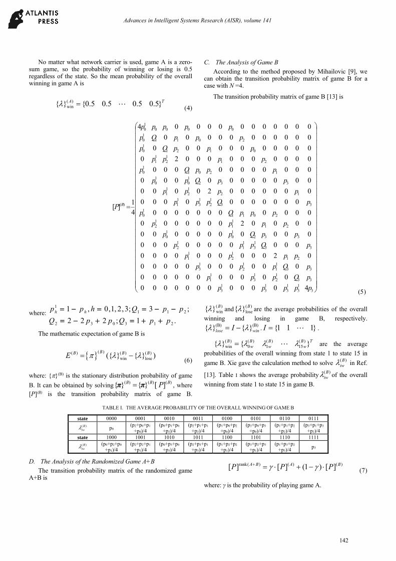
2) [P](A) in the fully-connected network: When game A uses the fully-connected network, any individual i can compete with all its neighbors. Taking p15 as an example, we explain the calculation method on the elements of this matrix. As game A is played between any two individuals, thus there are 62
4 C categories. From state 1 (0001) to state 5 (0101),
two cases exist. One is that individual 1 and individual 2 compete and individual 2 wins (The winning probability is 1/2), and the probability of occurrence is
12
1
2
1
6
1 . The
other is that individual 2 and individual 3 compete, individual 2 wins (The winning probability is 1/2), and the probability of occurrence is
12
1
2
1
6
1 .Therefore,
6
1
12
1
12
115 p . Then
other matrix elements can be calculated in the same way. Finally we can obtain the transition probability matrix of game A.
04141041000410000000
04112161121610012161000000
01214161121061012106100000
012112131012112112101211211210000
01211210416161012100061000
012101211213112112101210012112100
001211211211213112100121012101210
00061061614100012101211210
01211210121000416161061000
012101210121001213112112112112100
001211210012101211213112112101210
00061000121061614101211210
000012112112101211211210311211210
00000610121061012161411210
00000061121006112161121410
00000004100041041410
][ )(AP
The corresponding stationary distribution probability of game A is
{}(A)={0,1/20,1/20,1/10,1/20,1/10,1/10,1/20,1/20,1/10,1/10,1/20,1/10,1/20,1/20,0}.
141
Advances in Intelligent Systems Research (AISR), volume 141
No matter what network carrier is used, game A is a zero-sum game, so the probability of winning or losing is 0.5 regardless of the state. So the mean probability of the overall winning in game A is
TA }5.05.05.05.0{}{ )(
win
C. The Analysis of Game B
According to the method proposed by Mihailovic [9], we can obtain the transition probability matrix of game B for a case with N =4.
The transition probability matrix of game B [13] is
313
13
13
13
3312
13
11
3311
12
13
2112
11
3313
11
12
33210
10
2111
12
201110
3312
13
11
1212
11
33210
10
120110
2112
11
012110
201110
000010
)(
400000000000
00000000000
00000000000
020000000000
00000000000
00000000000
000020000000
00000000000
00000000000
000000020000
00000000000
00000000000
000000000020
00000000000
00000000000
000000000004
4
1][
ppppp
pQppp
pQppp
pppp
pQppp
ppQpp
pppp
pppQp
pQppp
pppp
ppQpp
pppQp
pppp
pppQp
pppQp
ppppp
P B
where: 1
1 1 2
2 3 0 3 1 2
1 , 0,1, 2,3; 3 ;
2 2 2 ; 1 .h hp p h Q p p
Q p p Q p p
The mathematic expectation of game B is
( )( ) ( ) ( )win lose({ } { } )
BB B BE
where: {}(B) is the stationary distribution probability of game
B. It can be obtained by solving )()()( ][}{}{ BBB Pππ , where [P](B) is the transition probability matrix of game B.
)(win}{ B and ( )
lose{ } B are the average probabilities of the overall
winning and losing in game B, respectively. (B) (B){ } { }lose winI . }111{ I .
TBw
Bw
Bw
B }{}{ )(15
)(1
)(0
)(win are the average
probabilities of the overall winning from state 1 to state 15 in
game B. Xie gave the calculation method to solve )(Biw in Ref.
[13]. Table I shows the average probability )(Biw of the overall
winning from state 1 to state 15 in game B.
TABLE I. THE AVERAGE PROBABILITY OF THE OVERALL WINNING OF GAME B
state 0000 0001 0010 0011 0100 0101 0110 0111 )(B
iw p0 (p2+p0+p1
+p0)/4 (p0+p1+p0
+p2)/4 (p2+p1+p1
+p2)/4 (p1+p0+p2
+p0)/4 (p3+p0+p3
+p0)/4 (p1+p1+p2
+p2)/4 (p3+p1+p3
+p2)/4 state 1000 1001 1010 1011 1100 1101 1110 1111
)(Biw (p0+p2+p0
+p1)/4 (p2+p2+p1
+p1)/4 (p0+p3+p0
+p3)/4 (p2+p3+p1
+p3)/4 (p1+p2+p2
+p1)/4 (p3+p2+p3
+p1)/4 (p1+p3+p2
+p3)/4 p3
D. The Analysis of the Randomized Game A+B
The transition probability matrix of the randomized game A+B is
)()()(rank ][)1(][][ BABA PPP
where: γ is the probability of playing game A.
142
Advances in Intelligent Systems Research (AISR), volume 141
According to (8), we deduce the stationary distribution
probability )(rank}{ BA of the randomized game A+B.
)()()( ][}{}{ BArankBArankBArank P ππ
The mathematical expectation of the game A+B
is )(rank BAE
rank ( )rank ( ) rank( ) rank( )win loseπ ({ } { } )
A BA B A B A BE
where: )(rankwin}{ BA and rank ( )
lose{ } A B
are the average
probabilities of the overall winning and losing in game A+B.
Moreover, rank( ) rank( ){ } { }A B A Blose winI .
}111{ I .
)(
win)(
win)(rank
win }{)1(}{}{ BABA
where: ){win}{ A and ){
win}{ B are the mean probabilities of the
overall winning in game A and game B.
The established conditions of the weak paradoxical form is
)()( BBArank EE
0)( BE
The established conditions of the strong paradoxical form is
0)( BArankE
0)( BE
E. The Analysis of Results
We take N=4 and get the mathematical expectation of game B according to [P](B) in (5) and
TBw
Bw
Bw
B }{}{ )(15
)(1
)(0
)(win in Table 1. Then, based
on [P](A)in (2) and (3) and [P](B) in (5), we obtain )(rank}{ BA
by using (7) and (8). Moreover, by substituting ){win}{ A in
(4)and ){win}{ B in (5) into (10), we get )(rank
win}{ BA . Finally,
we substitute )(rank}{ BA and )(rankwin}{ BA into (9) and obtain
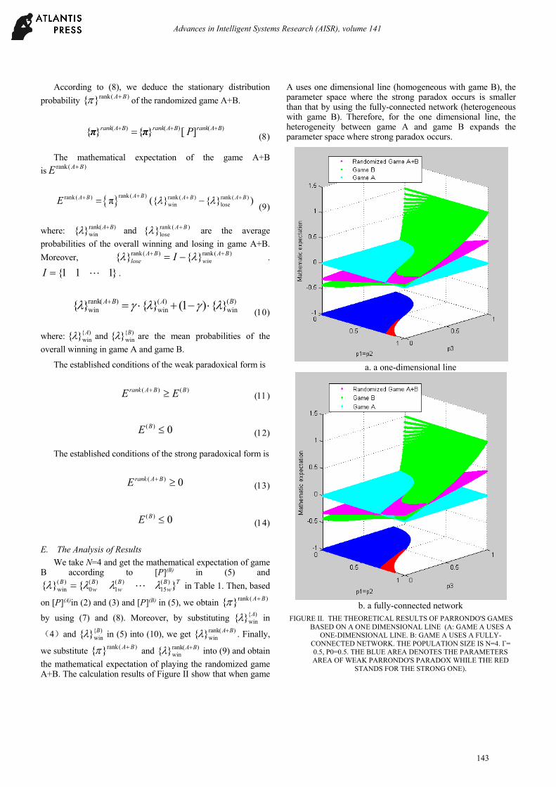
the mathematical expectation of playing the randomized game A+B. The calculation results of Figure II show that when game
A uses one dimensional line (homogeneous with game B), the parameter space where the strong paradox occurs is smaller than that by using the fully-connected network (heterogeneous with game B). Therefore, for the one dimensional line, the heterogeneity between game A and game B expands the parameter space where strong paradox occurs.
a. a one-dimensional line
b. a fully-connected network
FIGURE II. THE THEORETICAL RESULTS OF PARRONDO'S GAMES BASED ON A ONE DIMENSIONAL LINE (A: GAME A USES A
ONE-DIMENSIONAL LINE. B: GAME A USES A FULLY-CONNECTED NETWORK. THE POPULATION SIZE IS N=4. Γ= 0.5, P0=0.5. THE BLUE AREA DENOTES THE PARAMETERS AREA OF WEAK PARRONDO'S PARADOX WHILE THE RED
STANDS FOR THE STRONG ONE).
143
Advances in Intelligent Systems Research (AISR), volume 141

III. THE SIMULATION ANALYSIS BASED ON A TWO-DIMENSIONAL LATTICE
A. Model
The multi-agent model based on a two-dimensional lattice is shown in Figure III[16], where game B uses two dimensional lattice ( such a square lattice uses periodic boundary conditions, that is, the left and right edges are connected; the up and below edges are connected.). Game A uses the following networks: 1) a two-dimensional lattice (homogeneous with game B); 2) random network (heterogeneous with game B); a scale-free network (heterogeneous with game B); 4) a fully connected
network. On each round of game, one player ‘i’ is randomly chosen from N players to randomly play game A (probability γ) or B (probability 1-γ). When game A is played, individual j is chosen from i’s spatial neighbors randomly. Then the interaction between i and j is assumed in a competitive way. When game B is played, the winning or losing probability of individual i is dissimilar under different conditions of neighboring environment, which has five different kinds of winning and losing conditions. Therefore, game B is composed of 5 branches. The corresponding winning probabilities of the
individual i are hp (h=0,1,2,3,4).
FIGURE III. THE MULTI-AGENT PARRONDO’S MODEL BASED ON A TWO DIMENSIONAL LATTICE
B. Construction of Random Network
We use the rewiring mechanism [17] to generate random network. Based on the original square lattice, first a randomly chosen EF link is broken up and the site E is rewired to the randomly chosen site D (D cannot be the neighbor of E). This process is repeated K times. Compare random network with the original square lattice and the degree of the heterogeneity is determined by the rewiring times K.
C. Construction of a BA Scale-Free Network
To demonstrate the progressively changing from random network to scale-free network, we use an adjustable-parameter network of degree distribution and the corresponding construction method. The steps are in [18]: a) growth. The initial network consists of N nodes, where m0 nodes are fully connected among themselves. Thus, the set J2 is constructed; the unconnected set J1 is composed by ((N-m0) isolated nodes. At each time step, choose one new node from J1. In order to produce m edges, we connect this new node to some other nodes. b) preferential connectivity. m edges of the new node are connected to the nodes from the remaining (N-1) nodes with probability λ; then connect the nodes of the set J2 by following a linear preferential attachment strategy with the
probability 1-λ. When the connectivity is completed, we remove the new node from J1 and add it to J2. c) After N-m0
steps, the network model is generated by a series of parameter λ∈[0,1], where λ=0 corresponds to a BA scale-free network and λ=1 corresponds to random network.
D. The Calculation Results and the Analysis
For the two dimensional lattice, we also perform the theoretical analysis. Without generality, we analyze the case of N=9 at least (the 3×3 lattice network). With the increase of N, the transition probability matrix is added with 2N. Then, the analysis of the stationary distribution probability and the mathematical expectation becomes difficult. Therefore, for the two dimensional lattice, we mainly use computer simulations to analyze.
For computer simulations, we define the multi-agent average fitness d(t) as
T
tWtd
)()(
144
Advances in Intelligent Systems Research (AISR), volume 141

where:
N
ii CtCtW
10 ])([)( was the multi-agent total
profit. )(tCi was the capital of individual i at time t, C0 was
the initial capital and T was the total time of the game.
FIGURE IV. SIMULATION RESULTS (THE POPULATION SIZE N IS 1600 AND PLAYING TIME T IS 100 000. THE INITIAL WINNING
(1) AND LOSING (0) STATES ARE SET RANDOMLY. THE PROBABILITY OF PLAYING GAME A IS P=0.5 AND THE
PARAMETERS OF GAME B ARE P0=0.01, P1=0.15, P2=P3=0.7 AND P4=0.6. WE USE DIFFERENT RANDOM NUMBERS TO
PLAY THE GAME FOR 100 TIMES REPETITIVELY AND THEN MAKE A FIGURE FROM THE AVERAGE VALUE OF THEIR RESULTS. THE REWIRING TIMES K IS 1600 IN RANDOM
NETWORK.)
FIGURE V. THE EFFECT THAT THE HETEROGENIETY OF THE NETWORKS (THAT IS THE REWIRING TIMES K) HAS ON THE
POPULATION GAIN (THE NETWORK CARRIER OF GAME A CHANGES PROGRESSIVELY FROM REGULAR NETWORK TO RANDOM NETWORK WITH THE INCREMENT OF K. OTHER
PARAMETER ARE THE SAME AS IN FIGURE 4.)
Figure IV shows the simulation results of the average gain of the population, including playing game B individually (game
B uses a square lattice) and the randomized game A+B (where game A uses a square lattice, random network, a BA scale-free network and a fully-connected network, respectively). According to Figure IV, we notice that no matter what network game A uses, the gain of the randomized game A+B is positive, where Parrondo’s paradox occurs. Especially, the gain based on the square lattice is the largest. Therefore, for the square lattice, when game A and game B have the same network, they are conducive to increasing the gain of the game. In order to study the quantitative effect that the heterogeniety of the networks has on the gain, we use the method introduced in Section 2.2 by changing the rewiring times K. Figure V shows the effects that the rewiring times K has on the population profit for game A which changes gradually from regular network to random network. We find that with the increment of the degree of the heterogeniety between game A and game B, the gain decreases gradually until to stabilization.
Figure VI demonstrates the effects that the adjustable parameter λ of degree distributions has on the population gain. We see that the effect is not obvious, which shows that the heterogeneity of the networks has no obvious change when the network changes progressively from random network to a scale-free network.
FIGURE VI. THE EFFECT THAT Λ HAS ON THE AVERAGE GAIN OF THE POPULATION (THE NETWORK CARRIER CHANGES
GRADUALLY FROM A SCALE-FREE NETWORK TO RANDOM NETWORK WITH THE INCREMENT OF Λ. M0=2, M=2. OTHER
PARAMETERS ARE THE SAME AS IN FIGURE 4)
Figure VII shows the parameter space in which paradox occurs on the two-dimensional lattice. The calculation results demonstrate that when game A uses a two-dimensional lattice (heterogeneous with game B), the parameter space where the strong paradox occurs is slightly larger than that in other three networks while the parameter space where the weak paradox occurs is slightly smaller than that in other three networks. Therefore, for the two-dimensional network, homogeneousness between game A and game B enlarges the parameter space in strong paradox.
145
Advances in Intelligent Systems Research (AISR), volume 141

a. random network
b. two-dimensional lattice
c. BA scale-free network
d. fully-connected network
FIGURE VII. THE RESULTS OF PARRONDO'S GAME BASED ON TWO-DIMENSIONAL NETWORKS (A. GAME A USES TWO-
DIMENSIONAL LATTICE B. GAME A USES RANDOM NETWORK. THE REWIRING TIMES ARE 1600. C. GAME A USES
BA SCALE-FREE NETWORK. D. GAME A USES FULLY-CONNECTED NETWORK. THE POPULATION SIZE IS N=1600. Γ= 0.5. THE PARAMETERS OF GAME B ARE P1=0.15 AND
P2=P3=0.7. THE BLUE AREA DENOTES THE PARAMETERS AREA OF WEAK PARRONDO'S PARADOX WHILE THE RED
STANDS FOR THE STRONG ONE).
IV. CONCLUSIONS
For the cases that the spatial networks between game A and game B are different (heterogeneous networks), this paper demonstrates the effects of the heterogeneity of the networks through the theoretical analysis and computation simulations.
We perform the theoretical analysis on a one-dimensional line. Game A uses the following two networks: a one-dimensional line (homogeneous with game B) and a fully-connected network (heterogeneous with game B). We deduce the transition probability matrix of game A under these two networks and give the mathematical expectation of the randomized game A+B. The theoretical results show that when game A uses a one-dimensional line (homogeneous with game B, the parameter space where strong paradox occurs is smaller than that in fully-connected network (heterogeneous with game B). Therefore, for the one- dimensional line, the heterogeneity between game A and game B enlarges the parameter space where the strong paradox occurs.
We perform computer simulations on two-dimensional networks. Game A uses the following four networks: a two-dimensional lattice (homogeneous with game B), random network, a BA scale-free network and a fully-connected network (the latter three network are heterogeneous with game B). The simulation results show that when game A uses the two-dimensional lattice (homogeneous with game
146
Advances in Intelligent Systems Research (AISR), volume 141

B), the gain and the parameter space where the strong paradox occurs are both slightly larger than those in the other three networks. Moreover, the gain and the strong paradox space decrease with the increment of the degree of heterogeneity, which shows that the homogeneousness between game A and game B is beneficial for two-dimensional networks.
ACKNOWLEDGMENT
This project was supported by The Ministry of Education, Humanities and Social Sciences research projects (Grant No. 13YJAZH106 and 15YJCZH210); The Talent Project for Higher Education Promotion Program of Anhui Province; and Anhui Provincial Foundation for Outstanding Young Teachers in Higher Education Institutions, China (Grant No. 2013SQRL023ZD);Anhui Provincial Natural Science Foundation (Grant No. 1708085MF164).
REFERENCES [1] J. M. R. Parrondo, “How to cheat a bad mathematician, in EEC HC&M
Network on Complexity and Chaos (#ERBCHRX-CT940546), ” ISI, Torino, Italy, 1996,Unpublished.
[2] G. P. Harmer and D. Abbott, “Parrondo's paradox,” Statistical Science, vol. 14, pp. 206–213, 1999.
[3] G. P. Harmer and D. Abbott, “Losing strategies can win by Parrondo's paradox,” Nature, vol. 402, pp. 864,1999.
[4] D. Abbott, “Asymmetry and Disorder: A Decade of Parrondo's Paradox,” Fluctuation and Noise Letters, vol. 9, pp. 129–156, 2010.
[5] J. M. R. Parrondo, G. P. Harmer and D. Abbott, “New paradoxical games based on Brownian ratchets,” Physical Review Letters, vol. 85, pp. 5226–5229, 2000.
[6] R. J. Kay and N. F. Johnson, “Winning combinations of history-dependent games,” Physical Review E, vol. 67, pp. 056128, 2003.
[7] P. Arena, S. Fazzino, L. Fortuna and P. Maniscalco, “Game theory and non-linear dynamics: the Parrondo paradox case study,” Chaos Solitons & Fractals, vol. 17, pp. 545–555, 2003.
[8] R. Toral, “Cooperative Parrondo’s games,” Fluctuation and Noise Letters, vol. 1, pp. 7–12, 2001.
[9] Z. Mihailovic and M. Rajkovic, “One dimensional asynchronous cooperative Parrondo’s games,” Fluctuation and Noise Letters, vol. 3, pp. 389–398, 2003.
[10] Z. Mihailovic and M. Rajkovic, “Cooperative Parrondo’s games on a two- dimensional lattice,” Physica A, vol. 365, pp. 244–251,2006.
[11] C. Wang, N. G. Xie, L. Wang, Y. Ye and G. Xu, “A Parrondo’s paradox game depending on capital parity,” Fluctuation and Noise Letters, vol. 10,pp. 147–156, 2011.
[12] R. Toral, “Capital redistribution brings wealth by Parrondo's paradox,” Fluctuation and Noise Letters, vol. 2, pp. 305–311, 2002.
[13] N.G. Xie, Y. Chen, Y. Ye, G. Xu, L.G. Wang and C. Wang, “Theoretical analysis and numerical simulation of Parrondo’s paradox game in space,” Chaos, Solitons & Fractals, vol. 44, pp. 401–414, 2011.
[14] L. G. Wang, N. G. Xie, G. Xu, C. Wang, Y. Chen and Y. Ye, “Game-model research on coopetition behavior of Parrondo’s paradox based on network,” Fluctuation and Noise Letters, vol. 10, pp. 77–91, 2011.
[15] Y. Ye, N. G. Xie, L.G. Wang, L. Wang and Y. W. Cen, “Cooperation and competition in history-dependent Parrondo’s game on networks,” Fluctuation and Noise Letters, vol. 10, pp. 323–336, 2011
[16] Y. Ye, N. G. Xie, L. G. Wang, R. Meng and Y. W. Cen, “Study of biotic evolutionary mechanisms based on the multi-agent Parrondo's games,” Fluctuation and Noise Letters, vol. 11, pp. 352–364, 2012.
[17] G. Szabo, A. Szolnoki and R.Izsak, “Rock-scissors-paper game on regular small-world networks, ” Journal of Physics A:Mathematical and General, vol. 37, pp. 2599–2609, 2004.
[18] J. Gómez-Gardeñes and Y. Moreno, “From scale-free to Erdos-Rényi networks,” Physical Review E, vol. 73, pp. 645–666, 2006.
147
Advances in Intelligent Systems Research (AISR), volume 141