The effect of schooling on health: Evidence on several

health outcomes and behaviors in Italy

Michela Braga∗ Massimiliano Bratti†

This draft: December 16, 2016

Preliminary and Incomplete. Please do not cite.

Abstract

This paper investigates the non-pecuniary benefits of education using several in-

dividuals’ health outcomes, health-damaging and health-improving behaviors, and

preventive care. We exploit a reform which raised compulsory schooling by three

years in Italy to identify the causal effect of lower secondary education and, unlike

most previous papers in the literature, we analyze a wide range of health indicators.

Our analysis shows that the rise in schooling induced by the reform reduced BMI

and the incidence of obesity across Italian women, and raised men’s likelihood of

doing regular physical activity and cholesterol and glycemia checks. No effect is

found instead on preventive care and health-improving behavior for women, and on

smoking prevalence and intensity for both genders. Some potential reasons for the

gender differences in the results are discussed.

JEL codes. I12 I24

∗Bocconi University, via Rontgen 1, I-20136 Milan,Italy. E-mail: michela.braga@unibocconi.it†(corresponding author) DEMM, Universita degli Studi di Milano, via Conservatorio 7, I-20122 Milan,

Italy and IZA (Bonn), Ld’A (Milan). Phone: +39 02 503 21545. Fax: +39 02 503 21505. E-mail:

massimiliano.bratti@unimi.it

1

Keywords: compulsory schooling reform, education, health, health-related behav-

ior, schooling, Italy

2

1 Introduction

Non-communicable diseases (NCDs) are the primary cause of death in the world, and

account for 63% of the 57 million deaths that occurred in 2008 (WHO, 2011b). In most

middle- and high-income countries NCDs were responsible for more deaths than all other

causes of death combined. Almost all high-income countries report the proportion of

NCD deaths to total deaths to be more than 70%. In the same group of countries NCDs

accounted for 77% of the total number of years lost, compared to 7% for communicable

diseases and 11% for injuries (WHO, 2011a). Italy makes no exception in this respect

with an estimated 537,000 deaths due to NCDs, which represent 92% of total deaths

(WHO, 2011b).

In 2008, the leading causes of NCDs deaths were cardiovascular diseases, cancers,

respiratory diseases, including asthma and chronic pulmonary diseases, and diabetes.

Important behavioral risk factors of heart diseases and stroke include tobacco use, physical

inactivity and unhealthy diet (low fruit and vegetable intake), which are responsible for

about 80% of all coronary heart disease and cerebrovascular disease worldwide (WHO,

2011a).

As the incidence of health-risky behaviors tends to be higher among low educated

individuals, higher educated individuals tend to live longer and healthier lives (Cutler

and Lleras-Muney, 2010). This simple stylized fact has stimulated many researchers to

investigate the origins of such a positive association.

Theoretically, three main channels have been identified for the effect of education on

individual health and health-related behaviors. Grossman (1972) stressed the productive

efficiency argument. The underlying idea is that education directly affects the health

production function and that, given the same quantity of inputs, more educated indi-

viduals produce a higher stock of health than less educated ones. A second channel is

allocative efficiency : education alters the input mix in the health production function.

As Rosenzweig and Schultz (1983) put forward, this argument in its strongest form main-

3

tains that education will have no impact on health unless it changes the inputs in the

health production function, and the coefficient on education in this function would be

zero if all inputs were included. Hence, the main mechanism through which education

affects the input mix is by increasing health-related knowledge — e.g. on the harmful

effects of smoking — or the speed of adoption of health enhancing inputs.1 Finally, the

third variable hypothesis suggests instead that education is endogenous with respect to

health, because education and health choices are likely to be affected by the same set

of unobserved factors (Fuchs, 1982). To clarify this point consider the case of the in-

tertemporal discount rate. Individuals with a high discount rate are likely to invest less

in education and more likely to engage in health-damaging behavior, e.g., smoking, heavy

drinking. From the third variable hypothesis perspective, a negative correlation between

education and smoking stems from an unobserved variable, and does not reflect a true

causal relationship (see, for instance Farrell and Fuchs, 1982; Sander, 1998).

The last explanation suggests that care should be taken of the potential spurious

correlation between education and health owing to individual unobserved heterogene-

ity. For this reason, whereas early papers only reported simple associations between

education and health, researchers have recently adopted careful identification strategies

to assess the causal nature of the health-education gradient. In particular, recent work

is increasingly using instrumental variable (IVs) strategies (for a review, see Grossman,

2006) and fuzzy regression discontinuity (FRD) designs for identification. A very popular

‘instrument’ in this literature is the introduction of compulsory schooling age reforms.

This source of identification has been already exploited in a number of countries, includ-

ing the US (Adams, 2002; Glied and Lleras-Muney, 2003; Lleras-Muney, 2005), the UK

(Oreopoulos, 2006; Silles, 2009; Lindeboom et al., 2009; Clark and Royer, 2010), Den-

mark (Arendt, 2005), France (Albouy and Lequien, 2009), Germany (Kemptner et al.,

2011), Italy (Atella and Kopinska, 2011), the Netherlands (van Kippersluis et al., 2011),

and Sweden (Spasojevic, 2010; Meghir et al., 2012). Brunello et al. (2012) provides a

1Studies supporting this explanation of the effect of education include de Walque (2010) while evidencein Kenkel (1991) and Nerın et al. (2004) does not support this argument.

4

cross-section analysis using compulsory schooling reforms in several European countries.

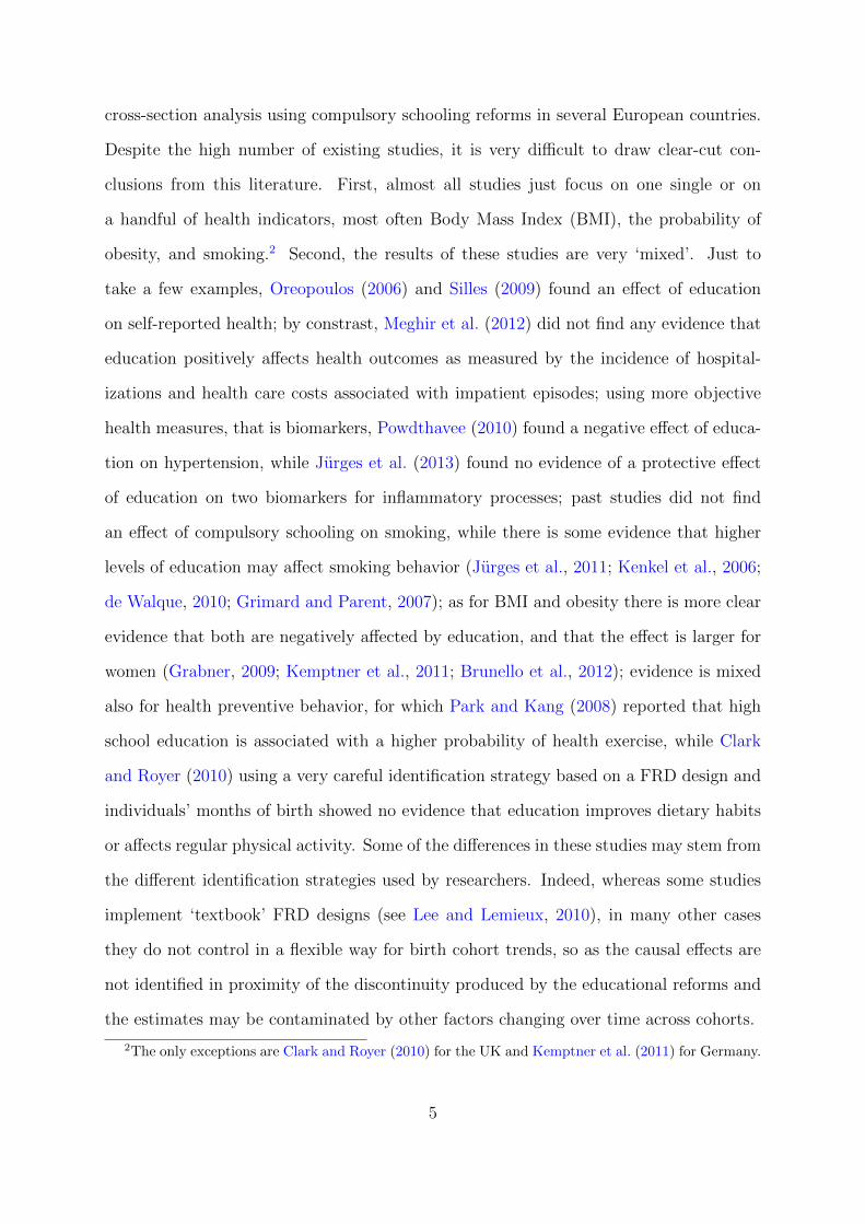
Despite the high number of existing studies, it is very difficult to draw clear-cut con-

clusions from this literature. First, almost all studies just focus on one single or on

a handful of health indicators, most often Body Mass Index (BMI), the probability of

obesity, and smoking.2 Second, the results of these studies are very ‘mixed’. Just to

take a few examples, Oreopoulos (2006) and Silles (2009) found an effect of education

on self-reported health; by constrast, Meghir et al. (2012) did not find any evidence that

education positively affects health outcomes as measured by the incidence of hospital-

izations and health care costs associated with impatient episodes; using more objective

health measures, that is biomarkers, Powdthavee (2010) found a negative effect of educa-

tion on hypertension, while Jurges et al. (2013) found no evidence of a protective effect

of education on two biomarkers for inflammatory processes; past studies did not find

an effect of compulsory schooling on smoking, while there is some evidence that higher

levels of education may affect smoking behavior (Jurges et al., 2011; Kenkel et al., 2006;

de Walque, 2010; Grimard and Parent, 2007); as for BMI and obesity there is more clear

evidence that both are negatively affected by education, and that the effect is larger for

women (Grabner, 2009; Kemptner et al., 2011; Brunello et al., 2012); evidence is mixed

also for health preventive behavior, for which Park and Kang (2008) reported that high

school education is associated with a higher probability of health exercise, while Clark

and Royer (2010) using a very careful identification strategy based on a FRD design and

individuals’ months of birth showed no evidence that education improves dietary habits

or affects regular physical activity. Some of the differences in these studies may stem from

the different identification strategies used by researchers. Indeed, whereas some studies

implement ‘textbook’ FRD designs (see Lee and Lemieux, 2010), in many other cases

they do not control in a flexible way for birth cohort trends, so as the causal effects are

not identified in proximity of the discontinuity produced by the educational reforms and

the estimates may be contaminated by other factors changing over time across cohorts.

2The only exceptions are Clark and Royer (2010) for the UK and Kemptner et al. (2011) for Germany.

5

In this paper, we seek to contribute to the previous literature in a number of ways.

First, thanks to a very specific health data source available for Italy we provide evidence

on the causal effects of lower secondary schooling on a very wide set of health variables.

Namely, we consider: (i) general health outcomes, such as chronic diseases and limita-

tions in activities of daily living; (ii) body-weight health outcomes, such as BMI, and

the probability of overweightness and obesity; (iii) ‘health-damaging’ behaviors, namely

current smoking status, average number of cigarettes smoked per day, probability of

ever smoking; (iv) ‘health-improving’ behaviors, in particular doing physical activity or

following a particular dietary regime; (v) health-preventive behaviors, namely the prob-

ability of having ever done a mammogram, a pap smear test or a Computerized Bone

Mineralometry (CBM), and cholesterol, glycemia and blood pressure check ups. Con-

sidering all these outcomes and behaviors together enables us to provide a more general

assessment of the effect of education on ‘health’ than most previous papers. Moreover,

as we report in the next section, the causal effect of education on the last two types of

behavior (health-improving and preventive behaviors) has been rarely investigated in the

literature.

Second, as we use the same identification strategy and the same data to examine all

health outcomes and behaviors, the differences in the causal effect of education among

outcomes and behaviors observed in our analysis are likely to reflect true differences rather

than being an artefact of adopting different identification strategies, or using different

data, like it may be the case when comparing the results of separate studies covering very

different health measures, data and empirical specifications.

Last but not least, in this paper we provide new causal evidence for Italy, for which

little evidence is available, using for identification a compulsory schooling reform imple-

mented in 1963. Among those exploited in the literature, the Italian reform is among

those which introduced the largest increase in the length of compulsory schooling (three

years, see Section 3). The new school obligation spanned the whole length of lower sec-

ondary education (grades 6-8), meaning that successful compliance with the reform led

6

individuals to achieve a higher educational qualification with respect to the past.3

The structure of the paper is as follows. Section 2 describes the data and section 3 the

identification strategy and the main features of the 1963 school reform, which provides

exogenous variation in individuals’ schooling, which is needed to identify causal effects.

The main results of our analysis are reported in section 4 and discussed in section 5.

Section 6 summarizes our main findings and concludes.

2 Data

We use micro data from the survey ‘Health conditions and use of health services’ (Con-

dizioni di salute e ricorso ai servizi sanitari) administered by the Italian National Statis-

tical Institute (ISTAT). For the sake of brevity we will refer to this survey as the Italian

Survey of Health (ISH, hereafter). At present, there are three waves of data, for the

1994, 1999 and 2004 years, respectively. This survey is a repeated cross section on a

yearly nationally representative sample of the Italian population. It collects information

on different aspects of everyday life at individual and household level and it has a specific

focus on health. Together with basic demographic characteristics, for individuals aged

at least 18, also information about health status, self-reported anthropometric measures,

smoking, dietary regimes, physical activity, health checkups, and use of health services

are collected. Anthropometric measures allow us to compute individual BMI that is de-

fined as the weight in kilograms divided by the height in square meters. According to

this index, the international standards classify individuals as severely underweight (BMI

below 16.5), normal weight (BMI over 16.5 up to 24.9), overweight (BMI from 25 up to

30) or obese (BMI over 30). A detailed description of all health outcomes and behaviors

analyzed in this paper is reported in Appendix.

Tables A1 and A2 in the Appendix report sample summary statistics by gender for

the dependent variables that we will use in our analysis.

3This is equivalent to junior school in the US context.

7

3 Identification strategy

In October 1963, Law n. 1859 December 31st, 1962 came into effect, increasing the

length of compulsory schooling from 5 (primary education) to 8 years (5 years of primary

education and 3 years of lower secondary education), and raising school-leaving age in

Italy. The law prescribed individuals to attend school at least until graduation from lower

secondary education, which usually took place at age 14. However, 15 years old children

with at least 8 years of schooling and without a low secondary education certificate were

exempted from the obligation. Enforcement of the law was far from being perfect initially,

and improved gradually, although it is necessary to wait until the mid ‘70s to observe

full compliance with the new school obligation (Checchi, 1997; Brandolini and Cipollone,

2002).

The individuals potentially affected by the reform were those aged less than 15 in

1963 and who did not have a lower secondary education diploma yet. For the initial

three cohorts affected by the reform, we expect the effect to be stronger for younger

cohorts. Indeed, those born in 1949 were required to stay only one additional year in

education, those born in 1950 two years, and those born in 1951 or later three years. It

must be noted that the reform might have created an incentive which goes beyond the

pure compliance with the new school obligation. Indeed, individuals who were missing

one or two years of education to comply with the obligation might have had an incentive

to also stay enrolled in the remaining grades of lower secondary education to complete the

cycle and attain the diploma. This additional incentive clearly depends on individuals’

birth cohorts. Last but not least, achieving a lower secondary education diploma can

be considered as a stronger treatment with respect to simply staying at school, since it

entailed passing a final exam, for which failure rates were rather high.

The 1963 reform not only increased age of compulsory education, but also the age at

tracking. Before the reform lower secondary schooling was divided into two tracks: the

vocational track and the academic track (scuola media, middle school). The vocational

8

track was chosen by individuals with lower socio-economic status who planned to quit

education after completing lower secondary schooling since it did not allow access to upper

secondary education, while the scuola media was chosen by those individuals who planned

to go on in education. After the reform, the two tracks were unified into a comprehensive

middle school (scuola media unica). Detracking of the school system is likely to have also

changed the peer group of compliers, that is for those individuals who in the absence of

the reform would have quit education at the minimum school leaving age, in the direction

of increasing the average quality of the peer group measured in terms of both ability and

socio-economic status. Detracking was not a distinctive feature of the Italian reform, but

it is common to many reforms increasing the length of compulsory schooling introduced

in other countries (and used in other papers), such as the UK, Denmark and Sweden.

The 1963 reform allows us to divide the Italian population between individuals who

were subject to the reform (the cohorts born from 1949 onwards) and those who were

not. This provides a potential source of identification to be exploited in a FRD design

(Lee and Lemieux, 2010). In particular, the reform created a discontinuity in lower

secondary schooling achievement. The design is ‘fuzzy’ since, like we said, compliance

with the reform was not perfect. The typical ‘compliers’ are those individuals who in the

absence of the reform would have quit education at the minimum legal age (11 years)

without a lower secondary school diploma. Using the reform for identification enables us

to estimate the causal effect of rising compulsory education on this specific subpopulation.

The results will be hardly generalizable to the whole population, but the subpopulation

of compliers is nonetheless an informative one as it comprises individuals who are more

likely to experience worse health outcomes (e.g., because they have higher intertemporal

discount rates), and for whom policy interventions may matter most.

In what follows, we describe in more detail our FRD design. Our identification strat-

egy can be described by a two-equation system, one equation for the outcome variable

(Y ) and one for the endogenous variable (D):

9

Y = a0 + τD + al1f(B − c) + (ar1 − al1) f(B − c)T + a2X + ε (1)

D = b0 + γT + bl1g(B − c) + (br1 − bl1) g(B − c)T + b2X + v (2)

where the individual subscript has been omitted, B is the individual birth cohort, c

is the pivotal cohort or cut-off point, i.e. the first birth cohort affected by the reform,

g(.) and f(.) are two polynomials in birth cohort (with the pivotal cohort normalized to

zero). D is an endogenous treatment dummy, corresponding to the fact of holding a lower

secondary education diploma, T ≡ I(B ≥ c) is a dummy for the reform eligibility (i.e.

B ≥ c), and X a vector of covariates. Among the covariates we included a quadratic term

in age, and year and region fixed effects.4 ε and v are two classical error terms and the as,

the bs, τ and γ the parameters to be estimated.5 We adopt here a ‘mixed approach’ to

implement the FRD, which is in between the ‘local linear regression’ and the ‘polynomial

approach’. The first approach can only be implemented with very large datasets (e.g.,

with Census data) so as even focusing on a few cohorts around the threshold one is likely

to have a sufficient number of observations. The second consists in using all the data

available, but specifying a flexible polynomial to capture cohort trends. We use a ‘local

polynomial approach’: we use a 10-year bandwidth around the pivotal cohort (the cohorts

from 1940 and 1960), which provides with a sufficient number of observations since there

are around 1,999 women and 1,963 men per cohort, however, we do not impose linearity

of the polynomial, but we select its degree using the procedure suggested by Lee and

Lemieux (2010). At the same time, our view is that the assumption that a polynomial

can properly control for all long-term unobserved factors changing between cohorts is

tenable only if we consider cohorts which are not too distant in time from the pivotal

4It is not possible to include a linear term in age as it is perfectly collinear with birth cohort trends,treatment status and year dummies. At the same time including the quadratic term in age is likely tocapture age-specific effects on health and health-related behaviors. The same is done, for instance, inKemptner et al. (2011).

5After centering the birth cohorts to c, i.e. the pivotal cohort, γ becomes the effect of the reform oneducational attainment.

10

cohort.

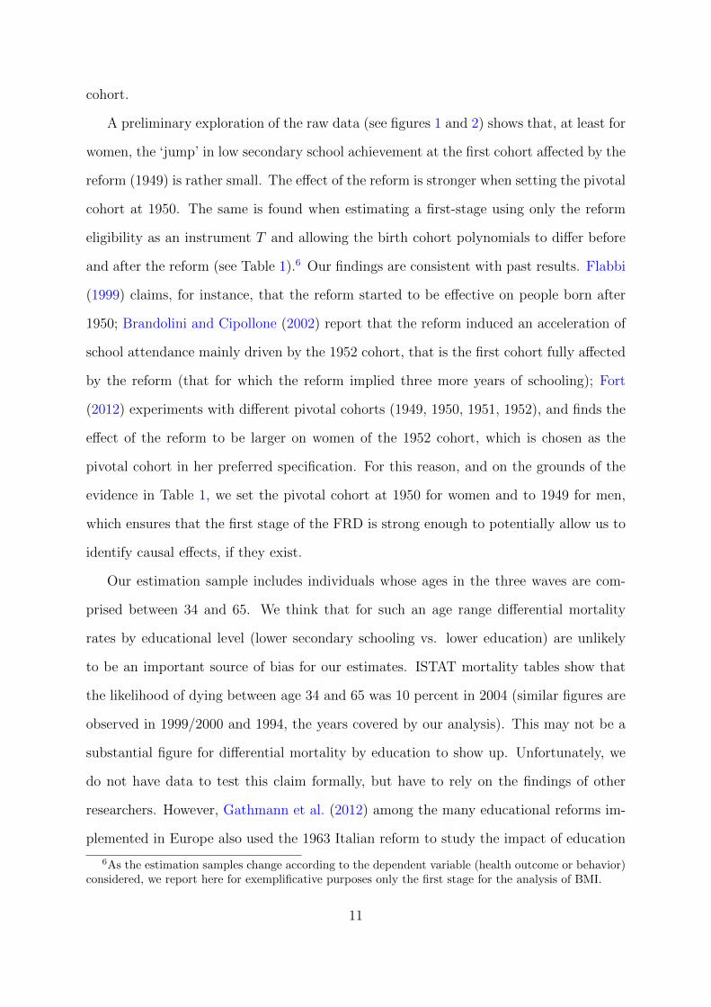
A preliminary exploration of the raw data (see figures 1 and 2) shows that, at least for

women, the ‘jump’ in low secondary school achievement at the first cohort affected by the

reform (1949) is rather small. The effect of the reform is stronger when setting the pivotal

cohort at 1950. The same is found when estimating a first-stage using only the reform

eligibility as an instrument T and allowing the birth cohort polynomials to differ before

and after the reform (see Table 1).6 Our findings are consistent with past results. Flabbi

(1999) claims, for instance, that the reform started to be effective on people born after

1950; Brandolini and Cipollone (2002) report that the reform induced an acceleration of

school attendance mainly driven by the 1952 cohort, that is the first cohort fully affected

by the reform (that for which the reform implied three more years of schooling); Fort

(2012) experiments with different pivotal cohorts (1949, 1950, 1951, 1952), and finds the

effect of the reform to be larger on women of the 1952 cohort, which is chosen as the

pivotal cohort in her preferred specification. For this reason, and on the grounds of the

evidence in Table 1, we set the pivotal cohort at 1950 for women and to 1949 for men,

which ensures that the first stage of the FRD is strong enough to potentially allow us to

identify causal effects, if they exist.

Our estimation sample includes individuals whose ages in the three waves are com-

prised between 34 and 65. We think that for such an age range differential mortality

rates by educational level (lower secondary schooling vs. lower education) are unlikely

to be an important source of bias for our estimates. ISTAT mortality tables show that

the likelihood of dying between age 34 and 65 was 10 percent in 2004 (similar figures are

observed in 1999/2000 and 1994, the years covered by our analysis). This may not be a

substantial figure for differential mortality by education to show up. Unfortunately, we

do not have data to test this claim formally, but have to rely on the findings of other

researchers. However, Gathmann et al. (2012) among the many educational reforms im-

plemented in Europe also used the 1963 Italian reform to study the impact of education

6As the estimation samples change according to the dependent variable (health outcome or behavior)considered, we report here for exemplificative purposes only the first stage for the analysis of BMI.

11

on mortality, and did not find any evidence of an effect for Italy.7

A peculiarity of our FRD design is that the discontinuity is defined on a discrete

variable (birth cohort). We follow Lee and Card (2008) and assume that the specification

error is the same at each side of the discontinuity. In this case, standard errors must be

clustered by birth cohort.

3.1 First-stage results: The effect of the 1963 reform on educa-

tional attainment

The FRD design can be implemented through two-stage least squares (2SLS). In this

section we comment in more details the results from the first-stage.

The reform was targeted to ‘marginal students’, those who would not have continued

in education in the absence of the increase of mandatory schooling age. These are also

the individuals who are less likely to continue in post-compulsory schooling after having

met the school obligation. For this reason, in the paper we limit our analysis only

to individuals who completed at most lower secondary schooling. As emphasized by

Lindeboom et al. (2009) focusing on the whole population, including in the estimation

sample also highly educated individuals which were not targeted by the reform, is likely

to reduce the estimated effect of the reform and generate a weak instrument problem.

Table 1 reports the first-stage of the FRD design. As we said, we set the pivotal

cohort to 1949 for men and to 1950 for women (columns 2 and 3). The table shows the

effect of the reform dummy, the cohort trends, the F-test on the excluded instrument and

7The evidence on the effect of education on mortality is mixed. Albouy and Lequien (2009) foundfor France that survival rates at 50 and 80 years old do not seem to be affected by years of schoolingbetween 13 and 16. Clark and Royer (2010), whose sample includes individuals under 70, found noevidence of a significant negative effect of compulsory education on mortality. By contrast, Cipolloneand Rosolia (2011) investigated the effect of a military service mass exemption —introduced following anearthquake— which increased high school completion in Southern Italy, and found that increasing by 1percentage point the proportion of high school graduates (corresponding to upper secondary schooling)reduces subsequent 10-year mortality rates (between the age 25 and 35) at the municipality level by 0.1-0.2 percentage points. However, they did not study the effect of lower secondary schooling. Last but notleast, van Kippersluis et al. (2011) did find a negative effect of compulsory schooling on mortality, butconsidering much older individuals than we do: for men surviving to age 81, an extra year of schoolingis estimated to reduce the probability of dying before the age of 89 by almost three percentage pointsrelative to a baseline of 50 percent.

12

the test suggested by Lee and Lemieux (2010) to select the order of the polynomial. The

first-stage does not show any sign of a weak instrument problem, although the instrument

is stronger on the female sample. The t−statistics are 6.2 for women and 4 for men, the

F-tests 37.19 and 16.1, respectively. The linear specification for the polynomial seems to

be appropriate for both genders, which was already evident in the figures 1 and 2. Indeed

in a linear regression including both a linear polynomial in birth cohort and birth cohort

dummies, the latter are jointly insignificant.

Overall, the reform seems to have produced a significant positive effect on the prob-

ability of completing lower secondary education, which amounts to 5.8 p.p. for women

and 4.1 p.p. for men. The reform was therefore more effective for women. These are

non-negligible effects, given that the last pre-reform birth cohorts in the estimation sam-

ple (1948 for men and 1949 for women) exhibit percentages of lower secondary school

achievement of 34.1% and 44.8%, for women and men, respectively.8 The magnitude of

the effect is comparable to the reforms used by Lleras-Muney (2005) for the US, but much

lower than for the UK reforms used by Clark and Royer (2010). This is not necessarily

a weakness of our study. Indeed, although we will able to estimate ‘more local’ treat-

ment effects, i.e. effects on a smaller subpopulation of compliers, in our case the Stable

Unit Treatment Value Assumption (SUTVA) —that is the absence of general equilibrium

effects— is more likely to hold. Like in Lleras-Muney (2005) but contrary to Clark and

Royer (2010), we may expect a substantial change in the peer group for the compliers

with the 1963 reform, and potentially strong peer effects.

In Table 2 we report the results of a ‘placebo experiment’, in which we check for

the presence of a discontinuity also in the likelihood of graduation from upper secondary

education in correspondence with the 1963 reform. The idea is that if there were some

concomitant unobserved factors (e.g., other concomitant reforms) which acted selectively

on the pivotal cohort, and increased its demand for both education and health, this should

have shown up also at higher levels of education. This can of course be considered as a

8Hence, the percentage of lower secondary educated women and men rose by about 17% and 9%,respectively.

13

‘placebo’ only if we do not expect any spillover of the reform on levels of education higher

than lower secondary schooling. This is credible given that the individuals complying

with the reform are likely to be the ‘marginal’ students. The dependent variable for

this analysis is a dummy which equals one if the individual completed upper secondary

schooling and zero if he/she achieved a lower level of education. The estimation sample is

restricted to individuals with upper secondary schooling or lower. As the table shows, no

discontinuity is present for upper secondary education, neither for women nor for men.9

This means that were no individuals that thanks to the reform acquired upper secondary

schooling.

4 Second-stage results

Before commenting on the results of the FRD design, we report as a benchmark the

OLS estimates for women and men in tables A3 and A4 in the Appendix, respectively.

For BMI, we find a negative association with education only for women (-1.071). By

contrast education is negatively associated with overweightness and obesity for both

genders. When we consider self-reported health measures (such as chronic illness, days

with limitations or in bed), they exhibit a negative correlation especially with women’s

education, while a negative association is found for men only for days spent in bed.

Education is significantly and positively associated with women’s smoking behavior, and

with men’s ever smoking. As for physical activity, the OLS estimates show a positive

coefficient on education for both genders. Considering special dietary regimes, education

is positively associated with men’s and women’s following a diet mainly for non-health

reasons. As for preventive behavior, for both women and men education is positively

associated with the probability of doing a number of health check ups. Since as widely

stressed in previous work, the OLS estimates are likely to suffer from the bias produced

by the endogeneity of education, in the remainder of this section we focus and comment

9Thus, including in the estimation sample also highly educated individuals would have greatly reducedthe power of the instrument and the precision of the 2SLS estimates.

14

on the FRD estimates only.

4.1 Health outcomes

Table 3 presents evidence on the causal effect of education on body-weight related out-

comes, in terms of BMI, overweightness and obesity, and on general health outcomes, in

terms of incidence and potential consequences of chronic diseases.

The estimates in Table 3 show that lower secondary schooling contributes to reducing

women’s BMI by 3.254, corresponding to -12.52 per cent (as the average female BMI for

women without lower secondary education in the estimation sample is 25.99). As lower

secondary schooling consists in Italy of three years of education, this roughly corresponds

to a -4.2 per cent reduction in BMI by one additional (‘effective’) year of education, a

magnitude which in line with the figure (4 per cent) reported by Grabner (2009) for

women in the US. The effect is precisely estimated and significant at the 1% statistical

level. An equally precise and sizeable negative effect is found also for women’s likelihood

of being obese, which falls by 24 per cent points (p.p.), but not for overweightness.

The same effects are not observed for men. Indeed, the point estimates are much

lower than for women, and never statistically significant.

Our result of a negative effect of lower secondary schooling on BMI and obesity only

for women is not new to the literature, and it is in line with findings in Brunello et al.

(2012), which report a protecting causal effect of years on education only for females

using data from several European countries. Grabner (2009) finds for the US an effect

which is stronger for women than for men.

In the following regressions we analyze whether lower secondary education decreases

the incidence of (self-reported and diagnosed) chronic diseases and limitations in activities

of daily living. For both men and women, the effects of education on the incidence of

chronic diseases go in the expected direction, while those on the number of days in which

individuals were limited in their daily activities or they spent in bed because of illness

15

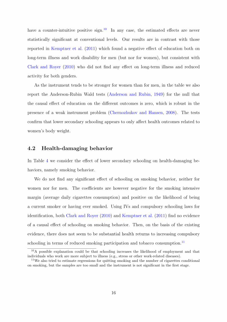
have a counter-intuitive positive sign.10 In any case, the estimated effects are never

statistically significant at conventional levels. Our results are in contrast with those

reported in Kemptner et al. (2011) which found a negative effect of education both on

long-term illness and work disability for men (but nor for women), but consistent with

Clark and Royer (2010) who did not find any effect on long-term illness and reduced

activity for both genders.

As the instrument tends to be stronger for women than for men, in the table we also

report the Anderson-Rubin Wald tests (Anderson and Rubin, 1949) for the null that

the causal effect of education on the different outcomes is zero, which is robust in the

presence of a weak instrument problem (Chernozhukov and Hansen, 2008). The tests

confirm that lower secondary schooling appears to only affect health outcomes related to

women’s body weight.

4.2 Health-damaging behavior

In Table 4 we consider the effect of lower secondary schooling on health-damaging be-

haviors, namely smoking behavior.

We do not find any significant effect of schooling on smoking behavior, neither for

women nor for men. The coefficients are however negative for the smoking intensive

margin (average daily cigarettes consumption) and positive on the likelihood of being

a current smoker or having ever smoked. Using IVs and compulsory schooling laws for

identification, both Clark and Royer (2010) and Kemptner et al. (2011) find no evidence

of a causal effect of schooling on smoking behavior. Then, on the basis of the existing

evidence, there does not seem to be substantial health returns to increasing compulsory

schooling in terms of reduced smoking participation and tobacco consumption.11

10A possible explanation could be that schooling increases the likelihood of employment and thatindividuals who work are more subject to illness (e.g., stress or other work-related diseases).

11We also tried to estimate regressions for quitting smoking and the number of cigarettes conditionalon smoking, but the samples are too small and the instrument is not significant in the first stage.

16

4.3 Health-improving behavior

In Table 4 we also consider the effect of lower secondary schooling on health-improving be-

haviors, namely doing physical exercise and following specific dietary regimes. Estimates

indicate that education does not have any causal effect on these behaviors for women.

By the contrary, on the male sub-sample, education translates into a higher probability

of doing regular exercise at least once a week, a lower probability of making very intense

exercise and a lower probability of following a particular dietary regime. This last re-

sult can be explained since if, on average, education induces individuals to have healthy

lifestyles, it may also reduce their need to follow a particular dietary regime. Our results

partially confirm those in Park and Kang (2008) who find a positive effect of education

on exercise for men in Korea, but they are not fully comparable since their dependent

variable takes value one for doing exercise or following a diet.

We make an attempt to go more in depth in the understanding of health-improving

behavior related to body weight by considering alternative dietary regimes prescribed for

health related problems. IHS survey contains information on individual nutrition habits.

In particular, individuals were asked whether they followed a diet with low fat and sugar

or low salt for health reasons or if they were used to having a specific dietary regime

for cultural reasons or for choice. Presumably, since more educated people are aware

of the benefits of healthy eating, they should adopt such behavior regularly and they

should have a lower need to follow a specific diet prescribing a low total intake of fats,

sugar, salt and sodium. The results are reported in Table 5. No evidence of the influence

of education also on these types of diet is found for women. By way of contrast, the

likelihood to follow an hypocaloric diet, a diet lower in salt or a specific diet prescribed

by a doctor is statistically lower among more educated men. This could partly explain

why more educated men also tend to do more regular physical activity than women: they

might have worse dietary habits.12 Men are more likely than women to choose alternative

dietary regimes and to adopt a diet but not for health reasons.

12Alternatively, they may be less in need of following these dietary regimes as they exercise regularly.

17

4.4 Preventive-care behavior

One strength of the IHS data is that it gathers very detailed information on the use of

health services, for which we can estimate the effect on health-preventive behavior.

The effect of lower secondary schooling on health-preventing behaviors is presented in

Table 6. In particular, we consider preventive medical examinations in absence of symp-

toms, regular health checkups and immunizations. For the checkups specific for women

(mammogram, pap smear and CBM tests) we find a marginally statistically significant

negative effect of education. For these outcomes, only descriptive evidence is available in

the literature (Cutler and Lleras-Muney, 2010, 2012; Wubker, 2012) pointing to a positive

association between education and the probability of check ups (such as mammograms,

pap smears and colonoscopy) or flu shots. At this stage further analysis is required to

better understand the underlying mechanism for such evidence. Considering the other

preventive behaviors, we do not find any significant effect of schooling for women. For

men, instead, compulsory lower secondary schooling increases the probability of having

regular checkups of glycemia and cholesterol levels. The effects are precisely estimated

and significant at the 1% statistical level. No effect is found for checks of blood pressure.

Also when considering the total number of preventive medical examinations in absence

of symptoms, the number of paid examinations or flu immunization no significant effect

is found, neither for men nor for women.

5 Discussion of the possible causal pathways

In the previous section we have shown significant negative effects of increasing compulsory

schooling on women’s BMI and obesity. A similar effect is not found for men. We have

also found evidence that education only affects some health-improving and preventing

behaviors of men but not of women. We explore in this section some potential reasons

for the gender differences observed in our analysis.

We would like to start this section with a cautionary note. For both women and men

18

we are estimating the causal effect of lower secondary schooling (the same ‘treatment’) on

health outcomes and behaviors. However, setting the pivotal cohorts to different years for

the two genders means that in the FRD design we are mainly exploiting the 1950 cohort

for women and the 1949 for men. Our first stage shows, indeed, that it took more time

to women to comply with the reform. This of course raises the question of why the 1949

female cohort reacted later to the reform. Now, if the reasons for this later compliance

were related to some unobservable characteristics interacting with health, and the effect

of education was heterogeneous according to these unobservables, then the differences in

the effects of education between genders may simply due to the fact that we are estimating

causal effects on two different sub-populations of compliers. In what follows, we abstract

from this potential objection, especially because we run separate analyses by gender so as

we are not directly comparing high-educated men with high-educated women, but high-

with low-educated women and high- with low-educated men. In this sense, objections

such as the existence of gender-specific investments on children should be less relevant in

our case compared to when an analysis pooling both genders is run.13

Let us start our comment on the effect of education on BMI and obesity. We explore

the following potential causal pathways which may explain why education has a protective

effect only for women:14

- income and the labor market returns to physical appearance;

- the ‘double burden’, that is educated women working simultaneously at home and

in the labor market;

- anxiety and depression;

- marital status and fertility.

13The first stage estimates whether belonging to a given cohort gives an advantage in terms of acquiringlower secondary education with respect to previous cohorts. Thus the mantaining assumption for makingcomparisons between men and women is that the 1949 female cohort is as close to the 1950 cohort interms of unobservables as the 1948 male cohort is to the 1949 cohort.

14See also the related discussion in Brunello et al. (2012).

19

A first explanation for the protective effect of education on BMI being observed only

for women may be related to the mediating effect of income. Sanz-de Galdeano (2005)

finds, for instance, that obesity declines more with increasing household income for women

than for men. A possible reason for the BMI-income gradient is that low income individ-

uals tend to eat cheap food, which is often high in fat and sugar, and therefore calories.

It is not clear though why this explanation should be relevant only for women and not

for men. Quintana Domeque and Villar (2009) stress how the income-BMI relationship

in nine European countries is negative for women and nonexistent for men. Moreover,

they find that the different relationship for men and women appears to be driven by the

negative association between BMI and own labor earnings for women. This is consistent

with women suffering a wage penalty associated with high BMI, and the association not

being mainly driven by eating ‘junk food’.15 Similar findings are reported in Gregory

and Ruhm (2011) showing that earnings peak for women at levels far below the clinical

threshold of obesity or even overweightness, which suggests that it is not obesity but

rather some other factor —such as physical attractiveness— that produces the observed

positive gradient between BMI and wages. As a consequence women may care more about

their body weight than men. The high-BMI wage penalty may also vary by level of ed-

ucation. The underlying idea is that while physical appearance matters less if a woman

is low educated and employed in a blue-collar job, it becomes important especially for

relatively more educated women, who are more frequently in white-collar jobs.

To investigate this hypothesis further we estimated a LPM model for an individual’s

labor force participation (LFP) status. The FRD estimates are reported in Table 7: for

both men and women education contributes to increasing labor force participation. The

estimated effect for men is however implausibly high, probably due to the weakness of

the instrument.16 We estimated with OLS a simple descriptive model of the link between

BMI and an individual’s LFP. LFP status seems to be more negatively associated with

15In which case a similar negative relationship between non-labor earnings and BMI should equallyemerge.

16The Kleibergen-Paap rk Wald F−statistic is 10.692, well below the Stock-Yogo weak identificationtest’s critical values, which is 16.38 for a 10% maximal IV size.

20

females’ than with males’ BMI. This is consistent with a greater mediating effect of

labor income —whatever the direction of causality is— for women than for men, but the

size of the effect is not large enough to explain the whole impact of education on BMI.

Indeed, women participating in the labor force have on average just a 0.3 lower BMI than

women out of the labor force. Probably, part of the effect is likely to be mediated by

differences in labor earnings conditional on labor force participation more than by LFP

status. Unfortunately, the ISH does not provide income or earnings data and we cannot

explore this hypothesis. In any case, as we have seen, the potential higher investments

in physical appearance for women do no show up in our analysis under the form of

voluntary physical exercise (regular or intense) or the probability of following specific

dietary regimes. The explanation that highly educated women may keep themselves in

good shape by consuming higher quality food, compared to men, seems instead to be

more in line with our empirical evidence, being consistent with both lower BMI and a

lower need for physical activity. Unfortunately, the ISH does not contain data to further

test this speculation.

A second possible explanation for the gender differences in the education-BMI gradient

is related to the so-called ‘double burden’ of educated women. Indeed, in Italy working

women must also take care of housework, and this may imply a higher consumption of

calories during the day. The ISH provides information on the degree of physical intensity

of housework and external work, which is expressed on a 3-point Likert scale: 1 for low,

2 for medium, and 3 for high. For each individual we summed the scores in the two

variables to obtain a joint indicator of the intensity of physical work at home and in the

job. Then we applied the usual FRD design using this dependent variable.17 The results

are reported in Table 7 and show an effect which is significant at the 10% level for women,

but much larger in magnitude and more precisely estimated for men. Thus, these results

do not help explain the gender gap. Moreover, from a simple OLS regression of BMI on

this indicator, reported in Table 8, the association appears to be very low and statistically

17Although the variable is not strictly cardinal, we use a simple linear model.

21

insignificant. We also built a dichotomous indicator for doing at least one of the following:

heavy work, heavy housework, heavy sport. This is very similar to the indicator used in

Brunello et al. (2012), and for which the authors found a higher effect of education for

women than for men (+10.8% and +4.5% increase in the probability of heavy activities,

for a one-year increase in education, for women and men respectively). However, also

in this case we do not observe any significant effect of low secondary education for both

genders (see Table 7). Thus the ‘double burden’ hypothesis does not seem to be the main

explanation for the gender differences observed in the BMI-education gradient.

Another explanation may be related to anxiety and depression, which are more fre-

quent among women. Education may positively contribute to an individual’s mental

health. This explanation is potentially relevant in our sample as simple OLS show a

strong positive association between having mental problems and female BMI (see Table

8). In particular, the ISH asked the following question: ‘in the last four weeks, did you

perform worse than you desired in the job or in house activities because of your emotional

state (e.g., depression or anxiety)?’. We adopted the FRD to estimate the effect of edu-

cation on emotional health. In spite of emotional health being an important correlate of

BMI, Table 7 does not show any significant effect of education on experiencing emotional

problems.18

Other two candidate explanations for the effect of education on BMI and the gender

gap may be (i) marital status ; (ii) fertility. As for the first, married individuals could

have a higher BMI, for instance because they are out of the marriage market. At the same

time education may have a negative effect on the likelihood of getting married (i.e. highly

educated individuals may be ‘choosy’). The positive association between marital status

and BMI is confirmed in Table 8, showing that married men and women have higher BMI

than singles, and that the ‘marriage gap’ in BMI is higher for women than for men (0.642

vs. 0.376). Table 7 reports the causal effect of education on the likelihood of being (or

18We also tried with another mental health indicator provided in the survey, corresponding to thequestion ‘In the last two weeks, did you experience a fall in concentration in the job or in daily activitiesbecause of your emotional state?’, and the results were very similar.

22

having been) married, estimated using the FRD design. The estimated coefficients are

negative but never statistically significant, and very similar across genders. As for the

second explanation, fertility, low educated women may have a higher fertility and gain

weight during pregnancy, with some of the weight gain being permanent. The ISH does

not collect information on total fertility but only on cohabiting children. For this reason,

and given the relatively high average age of the individuals included in our estimation

sample (many children may have left the parental home), it is not possible to estimate

the causal effect of education on fertility with our data.19 However, just to provide

some descriptive evidence, we checked if low educated mothers gain more weight during

pregnancy, and if weight gains are permanent. The ISH provides in each wave data on

the weight gained during pregnancy but only for mothers of children aged less than five.

We defined a dichotomous indicator for having gained more than 15 kg. and explored

the statistical association between education and this indicator, and the one between the

latter and current BMI (reported in Table 8), which both turned out to be statistically

insignificant. Thus weight gain during past pregnancies does not seem to be permanent,

and be positively associated with women’s current BMI.

Then, of all the various explanations put forward at the beginning of this section, only

the one related to the gender differences in the labor market returns to physical appear-

ance seems to have some potential for explaining the men-women gap in the protective

effect played by education on BMI and obesity.

As to preventive behaviors, we found significant positive effects of rising compulsory

schooling for glycemia and cholesterol checks for men. Here the men-women difference is

easier to explain as many health-risk factors are gender specific. There is a well established

evidence in medical sciences that the incidence of high blood pressure and hypertension

is higher among men than women and increases with age. In particular, the risk is

higher for men aged 45 or more, although according to the WHO in the last decades the

incidence is increasing also among younger men and women because of the significant

19A recent study by Fort (2012) uses for identification the same reform used in this paper and doesnot find significant effects of increasing compulsory schooling on completed fertility of Italian women.

23

changes in population lifestyle. No similar evidence is available for diabetes, since Type 1

diabetes has almost the same incidence among men and women, while Type 2 diabetes is

more common in older and overweight people with no gender difference. This evidence is

confirmed also by the last available national statistics for Italy. According to the Italian

National Statistical Institute (ISTAT), among men cardiovascular diseases were the first

cause of death in 2009 and also in the previous years, although the incidence is higher for

women. No difference emerges among genders for diabetes nor as a cause of death nor

as illness. Yet what is more difficult to rationalize is why a significant effect of education

shows up only for some health checks, especially for men, and not for others, for instance

for mammograms, paper smear tests and CBM for women. It is difficult to give a definitive

answer to this question with our data. We limit ourselves to saying here that it may due

to the consciousness-raising campaigns which were widespread for specific NCDs diseases

such as breast cancer, and which might have reached most women irrespective of their

levels of education and socio-economic status (Whynes et al., 2007). Women may be more

responsive than men to these campaigns or to health information in general, and education

may accordingly play a less important role for women than for men. Alternatively, there

might be gender differences in the effect of education on health risk perception. Last but

not least, also the ages at which the effects on preventive behaviors are identified may be

important. In particular, the pivotal cohort for men (1949) is observed at the age of 45,

49 and 55 in the 1994, 1999 and 2004 waves, respectively. These are the ages at which

the risk of hypertension and high blood pressure increase, and men of these ages may be

particularly sensitive in terms of behavior. Our data are not suitable to give a definitive

answer to these questions, and we leave a deeper investigation of these important issues

for future work.

24

6 Concluding remarks

In this paper we have used three waves of a very rich health survey for Italy gathering a

wealth of information on individuals’ health, health-related behaviors and use of health

services. This survey, combined with a ‘quasi-natural’ experiment represented by an

increase in compulsory schooling age introduced in 1963, enables us to analyze the causal

effects of lower secondary schooling on a very wide range of health-related variables.

Our analysis suggests that lower secondary schooling reduced BMI and the incidence

of obesity among Italian women, while no effect is found for men, and is in line with

the recent literature. Furthermore, we find no evidence that education reduced health-

damaging behaviors, such as smoking, neither for women nor for men.

As for health-improving behavior (i.e. healthy lifestyles) we only find a positive causal

effect of education on men, for whom it increased the likelihood of doing regular physical

exercise. Education also improved some health-preventive behaviors of men, by raising

the probability of cholesterol and glycemia checkups in the last year.

We provide some tentative explanations related to the gender differences in the rela-

tionship between education and BMI, and preventive behavior. As for the former, our

analysis allows us to discard many potential pathways and we put forward that the dif-

ferences may be related to the higher labor market returns to physical attractiveness

existing for women, while do not seem to be mediated by the fact that highly educated

women have a ‘double burden’ in terms of job and housework (consuming more calories),

by mental health, marital status or fertility behavior. As for the differences in preven-

tive behaviors, they could be explained by the gender specificity of many health risk

factors, and the wide diffusion of awareness-rising campaigns for female-specific NCDs

such as breast cancer, which might have provided valuable information to most individ-

uals irrespective of their educational levels. However, further research is needed to fully

understand the origin of these gender differences in the education-health gradient.

25

Acknowledgements

We thank participants to the ‘Second Lisbon Research Workshop on the Economics,

Statistics and Econometrics of Education’ (Lisbon, 2013), the RES 2013 annual confer-

ence (London), the ESPE 2013 conference (Aarhus) and the 22nd European Workshop on

Econometrics and Health Economics (Rotterdam), in particular our discussant Hans van

Kippersluis, for useful comments. Funding from the Seventh Framework Programme’s

project ‘Growing inequalities’ impacts’ (GINI) is gratefully acknowledged. All remaining

errors are ours.

References

Adams, S., 2002. Educational attainment and health: Evidence from a sample of older

adults. Education Economics 10, 97–109.

Albouy, V., Lequien, L., 2009. Does compulsory education lower mortality. Journal of

Health Economics 28, 155–168.

Anderson, T. W., Rubin, H., 1949. Estimation of the parameters of a single equation in a

complete system of stochastic equations. Annals of Mathematical Statistics 20, 46–63.

Arendt, J., 2005. Does education cause better health? A panel data analysis using school

reforms for identification. Economics of Education Review 24, 149–160.

Atella, V., Kopinska, J. A., 2011. Body weight of Italians: the weight of education.

CHILD Working Papers n. 10/2011. Turin: CHILD.

Brandolini, A., Cipollone, P., 2002. Return to education in italy 1992-1997. Bank of Italy,

Research Department,.

Brunello, G., Fabbri, D., Fort, M., 2012. The causal effect of education on body mass:

Evidence from Europe. Journal of Labor Economics forthcoming.

26

Checchi, D., 1997. L’efficacia del sistema scolastico italiano in prospettiva storica. In:

L’Istruzione in Italia solo un pezzo di carta? Il Mulino, Bologna.

Chernozhukov, V., Hansen, C., 2008. The reduced form: A simple approach to inference

with weak instruments. Economics Letters 100, 68–71.

Cipollone, P., Rosolia, A., 2011. Schooling and youth mortality: Learning from a mass

military exemption. CEPR Discussion Papers 8431, C.E.P.R. Discussion Papers.

Clark, D., Royer, H., 2010. The effect of education on adult health and mortality: evidence

from Britain. NBER Working Paper No. 16013. Cambridge (MA): NBER. Forthcoming

in the American Economic Review.

Cutler, D., Lleras-Muney, A., 2010. Understanding differences in health behaviors by

education. Journal of Health Economics 29, 1–28.

Cutler, D. M., Lleras-Muney, A., 2012. Education and health: insights from international

comparisons. NBER Working Paper No. 17738. Cambridge (MA): NBER.

de Walque, D. ., 2010. Education, information and smoking decisions: Evidence from

smoking histories in the United States, 1940-2000. Journal of Human Resources 45,

682–717.

Farrell, P., Fuchs, V., 1982. Schooling and health: The cigarette connection. Journal of

Health Economics 1, 217–230.

Flabbi, L., 1999. Returns to schooling in italy ols, iv and gender differences. Working

Paper 1, Universita Bocconi. Serie di Econometria ed Economia Applicata.

Fort, M., 2012. Empirical evidence on the role of education in shaping female fertility

patterns. mimeo.

Fuchs, V., 1982. Time preference and health: An explanatory study. In: Fuchs, V. (Ed.),

Economic Aspects of Health. University of Chicago Press, pp. 93–120.

27

Gathmann, C., Jurges, H., Reinhold, S., 2012. Compulsory schooling reforms, educa-

tion and mortality in twentieth century Europe. CESifo Working Paper Series 3755,

forthcoming on Social Science and Medicine.

Glied, S., Lleras-Muney, A., 2003. Health inequality, education and medical innovation.

NBER Working Paper No. 9738. Cambridge (MA): NBER.

Grabner, M., 2009. The causal effect of education on obesity: Evidence from compulsory

schooling laws, university of California, Davis.

Gregory, C. A., Ruhm, C. J., 2011. Where does the wage penalty bite? In: Economic

Aspects of Obesity. University of Chicago Press.

Grimard, F., Parent, D., 2007. Education and smoking: Were Vietnam war draft avoiders

also more likely to avoid smoking? Journal of Health Economics 26, 896–892.

Grossman, M., 1972. On the concept of health capital and the demand for health. Journal

of Political Economy 80, 223–255.

Grossman, M., 2006. Education and nonmarket outcomes. In: Hanushek, E., Welch, F.

(Eds.), Handbook of the Economics of Education. Elsevier, Amsterdam, Ch. 10, pp.

577–633.

Jurges, H., Kruk, E., Reinhold, S., April 2013. The effect of compulsory schooling on

healthevidence from biomarkers. Journal of Population Economics 26 (2), 645–672.

Jurges, H., Reinhold, S., Salm, M., 2011. Does schooling affect health behavior? Evidence

from the educational expansion in Western Germany. Economics of Education Review

30, 862–872.

Kemptner, D., Jurges, H., Reinhold, S., 2011. Changes in compulsory schooling and the

causal effect of education on health. Journal of Health Economics 30, 340–354.

Kenkel, D., 1991. Health behavior, health knowledge, and schooling. Journal of Political

Economy 99, 287–305.

28

Kenkel, D., Lillard, D., Mathios, A., 2006. The roles of high school completion and GED

receipt in smoking and obesity. Journal of Labor Economics 24, 635–660.

Lee, D. S., Card, D., 2008. Regression discontinuity inference with specification error.

Journal of Econometrics 14, 655–674.

Lee, D. S., Lemieux, T., 2010. Regression discontinuity designs in economics. Journal of

Economic Literature 48, 281–355.

Lindeboom, M., Liena-Nozal, A., van der Klaauw, B., 2009. Parental education and child

health: Evidence from a schooling reform. Journal of Health Economics 28, 109–131.

Lleras-Muney, A., 2005. The relationship between education and adult mortality in the

United States. Review of Economic Studies 72, 189–221.

Meghir, C., Palme, M., Simeonova, E., 2012. Education, health and mortality: evidence

from a social experiment. NBER Working Paper No. 17932. Cambridge (MA): NBER.

Nerın, I., Guillen, D., Mas, A., Crucelaegui, A., 2004. Evaluation of the influence of

medical education on the smoking attitudes of future doctors. Arch Bronconeumol 40,

341–347.

Oreopoulos, P., 2006. Estimating average and local average treatment effects of education

when compulsory schooling laws really matter. American Economic Review 96, 152–

175.

Park, C., Kang, C., 2008. Does education induce healthy lifestyle? Journal of Health

Economics 27, 1516–1531.

Powdthavee, N., 2010. Does education reduce the risk of hypertension? Estimating the

biomarker effect of compulsory schooling in england. Journal of Human Capital 4,

173–202.

Quintana Domeque, C., Villar, G., 2009. Income and body mass index in europe. Eco-

nomics & Human Biology 7, 73–83.

29

Rosenzweig, M., Schultz, T., 1983. Estimating a household production function: Het-

erogeneity, the demand for health inputs, and their effects on birth weight. Journal of

Political Economy 91, 723–746.

Sander, W., 1998. The effects of schooling and cognitive ability on smoking and marijuana

use by young adults. Economics of Education Review 17, 317–324.

Sanz-de Galdeano, A., 2005. The obesity epidemic in europe. IZA Discussion Paper No.

1814, IZA (Bonn).

Silles, M. A., 2009. The causal effect of education on health: Evidence from the United

Kingdom. Economics of Education Review 28, 122–128.

Spasojevic, J., 2010. Effects of education on adult health in Sweden: Results from a

natural experiment, in. In: Slottje, D., Tchernis, R. (Eds.), Current Issues in Health

Economics. Vol. 290 of Contributions to Economic Analysis. Emerald Group Publishing

Limited, Ch. 9, pp. 179–199.

van Kippersluis, H., O’Donnell, H., van Doorslaer, H., 2011. Long-run returns to edu-

cation. does schooling lead to an extended old age? Journal of Human Resources 46,

695–721.

Wubker, A., 2012. Who gets a mammogram amongst European women aged 50-69 years

and why are there such large differences across European countries? Health Economics

Review 2, 1–13.

WHO, 2011a. Global status report on noncommunicable diseases 2010. World Health

Organization, Geneva.

WHO, 2011b. Noncommunicable diseases country profiles 2011. World Health Organiza-

tion, Geneva.

Whynes, D. K., Philips, Z., Avis, M., 2007. Why do women participate in the english

cervical cancer screening programme? Journal of Health Economics 26, 306–325.

30

Appendix: Definition of health outcomes and behav-

iors

In our empirical analysis, we consider several health outcomes and behaviors defined as

follows:

� Health Outcomes

Chronic diseases. The survey asks for the presence of specific chronic diseases.

Although the questions changed a bit across waves, all three waves ask for the

presence of the following health conditions: asthma, allergy, diabetes, cataract,

hypertension, heart attack, angina pectoris, other heart disease, ictus, bronchitis,

arthrosis, osteoporosis, ulcer, malignant tumor, migraine, stones (liver or kidney),

cirrhosis. For each disease, two measures are provided, one for the diseases being

self-reported and the other for the diseases being diagnosed by a doctor (also in

this case the source is survey and not administrative hospital data). We defined

accordingly two dummy variables, one for the presence of at least one of the above

self-reported diseases, and one for these diseases being diagnosed.

Limitations in activities of daily living. The survey gathers information on the

number of days during the last four weeks individuals were limited from doing

activities of daily living or were constrained in bed.

Body Mass Index (BMI). Individuals self-reported their height (in meters) and their

body weight (in kilograms), from which it is possible to build a measure of BMI.

Overweightness. This is defined as BMI being greater than or equal to 25.

Obesity. This is defined as BMI being greater than 30.

� Health-damaging behavior

Current smoking status. Individuals were asked their current smoking status. We

define a dummy variable which equals one if an individual is a current smoker and

31

zero otherwise.

Average number of cigarettes smoked per day. Current smokers were asked the

average number of cigarettes smoked per day. The number of cigarettes is set to

zero for current non-smokers.

Ever smoked. This is a dummy variable which equals one if an individual is either

a current smoker or smoked in the past and zero otherwise.

� Health-improving behavior

Intense physical activity. Individuals were asked if, in their spare time, they did

intense physical activity (such as agonistic sports, fast running or biking) at least

once a week and for how long. Although the data have been collected in all the

waves, they are publicly available for research only for the last two waves.

Regular physical activity. Individuals were asked if, in their free time, they did

regular physical activity (such as going to the gym, running, biking up to a level

where they sweat a bit) at least once a week and for how long. Although the data

have been collected in all the waves, they are publicly available for research only

for the last two waves.

Any physical activity. From the previous two questions and combining an additional

item about doing soft physical activity (such as walking at least one kilometer

or doing soft exercise) we generate a dummy variable taking value one for those

individuals doing at least once a week any type of physical activity.

Dietary regime. All the waves collected information on the specific dietary regime

(if any) followed by the respondents. In particular, we have information on the type

of diet usually followed (i.e. low salt, low fat, low sugar, vegetarian, macrobiotic)

and the reasons why it has been chosen. From these questions, we defined one

dummy variable for having a ‘special’ dietary regime.

� Preventive-care behavior

32

Mammogram. Women were asked if they ever had a mammogram.

Pap smear test. Women were asked if they ever had a pap smear test.

CBM. Women were asked if they ever had a CBM.

Glycemia check, cholesterol check, blood pressure check. Individuals were asked if

they had regular glycemia, cholesterol and blood pressure checks, when was the last

one and why they did this check. The questions are slightly different from one wave

to the other, but we were able to construct a dummy variable taking value one if

the respondent had a check in the last year.

Diagnostic medical examinations. Individuals were asked if they had medical ex-

aminations in the last 4 weeks, their typology and the reason why they had these

visits. From these questions we construct a variable with the number of diagnostic

medical examinations made in absence of any particular symptom. The number of

preventive exams is set to zero for individuals who had no exams.

Paid examinations. This variable indicates the number of paid preventive exami-

nations.

Flu immunization.This variable takes value one for those individuals who had a flu

shot in the last year.

33

Figure 1: Effect of the 1963 reform on women’s likelihood to complete lower secondaryschooling

Note. In the top graph the pivotal cohort (i.e. the first cohort affected by the reform) is set to 1949 and

in the bottom graph to 1950. The data plotted refer to the estimation sample in Table 1 and includes

women in the IHS born between 1940 and 1960 with at most lower secondary schooling (and non-missing

covariates). Estimated linear trends are super-imposed to the scatter plot.

34

Figure 2: Effect of the 1963 reform on men’s likelihood to complete lower secondaryschooling

Note. In the top graph the pivotal cohort (i.e. the first cohort affected by the reform) is set to 1949 and

in the bottom graph to 1950. The data plotted refer to the estimation sample in Table 1 and includes

men in the IHS born between 1940 and 1960 with at most lower secondary schooling (and non-missing

covariates). Estimated linear trends are super-imposed to the scatter plot.

35

Table 1: First-stage results: Probability of attaining lower secondary schooling

women women men menc = 1949 c = 1950 c = 1949 c = 1950

T ≡ I(B ≥ c) 0.033*** 0.058*** 0.041*** 0.030*(0.011) (0.009) (0.010) (0.015)

g(B − c) -0.011 -0.009 0.017* 0.020**(0.007) (0.007) (0.009) (0.009)

g(B − c)× T 0.026*** 0.024*** 0.010*** 0.008**(0.002) (0.002) (0.002) (0.003)

F-test linear cohort trend vs. birth cohort dummies(a) 1.32 [0.17] 1.30 [0.18] 0.87 [0.61] 1.36 [0.14]F-test treated T= 0 9.60 [0.01] 37.19 [0.00] 16.01 [0.00] 3.91 [0.06]R2 0.178 0.178 0.162 0.162N. obs. 28896 28896 24965 24965

*** significant at 1%; ** significant at 5%; * significant at 10%.

(a) Test that birth cohort dummies are jointly equal to zero in a specification including both a linear poly-nomial in birth cohort and cohort dummies (Lee and Lemieux, 2010).Note. c stands for the ‘pivotal cohort’ (cutoff) and T is the dummy defining eligibility to the 1963 reform.g(B−c) and g(B−c)×T are the pre- and post-reform trends. P -values in brackets. Standard errors clusteredby birth cohort in parentheses. The table presents results setting the cutoffs at different cohorts. All first-stage estimates also include region and year fixed effects and a quadratic term in age and are estimated onindividuals for the birth cohorts 1940-1960 who attained no more than lower secondary schooling.

36

Table 2: First-stage placebo: Probability of attaining upper secondary schooling

women menc = 1949 c = 1950

T ≡ I(B ≥ c) 0.006 -0.003(0.006) (0.007)

g(B − c) 0.117*** 0.093***(0.005) (0.005)

g(B − c)× T -0.016*** -0.018***(0.002) (0.001)

R2 0.192 0.214N. obs. 33711 30213

*** significant at 1%; ** significant at 5%; * significant at 10%.

Note. P -values in brackets. Standard errors clustered by birth cohort in parentheses. All first-stage estimatesalso include region and year fixed effects and a quadratic term in age. The regressions are estimated onindividuals for the birth cohorts 1940-1960 who attained no more than upper secondary schooling.

37

Tab

le3:

Eff

ect

ofed

uca

tion

onhea

lth

outc

omes

Typ

eof

hea

lth

outc

ome

Ou

tcom

eG

end

erF

irst

-sta

ge

Sec

on

d-s

tage

N.

coeffi

cien

tF

-tes

t(a)

An

der

son

-Ru

bin

test

(b)

coeffi

cien

tob

serv

ati

on

s(δ

)(τ

)

Weightrelatedoutcomes

BM

IW

om

en0.0

58***

38.4

211.9

2-3

.254***

28896

(0.0

09)

[0.0

0]

[0.0

0]

(1.0

53)

Men

0.0

41***

16.0

10.0

5-0

.263

24965

(0.0

10)

[0.0

0]

[0.8

3]

(1.1

72)

Ove

rwei

ghtn

ess

Wom

en0.0

58***

38.4

22.2

0-0

.285

28896

(0.0

09)

[0.0

0]

[0.1

5]

(0.1

95)

Men

0.0

41***

16.0

10.0

2-0

.041

24965

(0.0

10)

[0.0

0]

[0.8

8]

(0.2

53)

Ob

esit

yW

om

en0.0

58***

38.4

211.8

9-0

.243***

28896

(0.0

09)

[0.0

0]

[0.0

0]

(0.0

63)

Men

0.0

41***

16.0

10.8

2-0

.144

24965

(0.0

10)

[0.0

0]

[0.3

8]

(0.1

47)

Gen

eralhealthoutcomes

Ch

ron

icil

lnes

s(s

elf-

rep

ort

ed)

Wom

en0.0

58***

37.1

90.4

9-0

.135

28922

(0.0

09)

[0.0

0]

[0.4

8]

(0.1

86)

Men

0.0

41***

16.0

31.5

5-0

.457

24985

(0.0

10)

[0.0

0]

[0.2

3]

(0.3

44)

Ch

ron

icil

lnes

s(d

iagn

osed

)W

om

en0.0

58***

37.1

92.3

5-0

.264*

28922

(0.0

09)

[0.0

0]

[0.1

4]

(0.1

60)

Men

0.0

41***

16.0

31.2

5-0

.444

24985

(0.0

10)

[0.0

0]

[0.2

8]

(0.3

62)

Day

sw

ith

lim

itat

ion

s(l

ast

4w

eeks)

Wom

en0.0

58***

37.1

90.1

80

.690

28922

(0.0

09)

[0.0

0]

[0.6

8]

(1.6

51)

Men

0.0

41***

16.0

30.1

20.8

16

24985

(0.0

10)

[0.0

0]

[0.7

3]

(2.2

72)

Day

sin

bed

(las

t4

wee

ks)

Wom

en0.0

58***

37.1

90.7

50.9

66

28922

(0.0

09)

[0.0

0]

[0.4

0]

(1.1

17)

Men

0.0

41***

16.0

30.0

70.4

40

24985

(0.0

10)

[0.0

0]

[0.8

0]

(1.6

83)

***

sign

ifica

nt

at1%

;**

sign

ifica

nt

at5%

;*

sign

ifica

nt

at

10%

.(a

)F

-tes

tfo

rth

eex

clu

sion

ofth

ere

form

du

mm

yT

inth

efi

rst

stage.

(b)

An

der

son

-Ru

bin

Wal

dte

stfo

rro

bu

stin

fere

nce

inth

ep

rese

nce

of

wea

kin

stru

men

ts(t

he

nu

llhyp

oth

esis

isτ

=0).

Not

e.T

he

colu

mn

‘firs

t-st

age’

rep

orts

the

coeffi

cien

tof

the

inst

rum

ent

(ref

orm

elig

ibil

ity)

an

dth

eco

lum

n‘s

econ

d-s

tage

the

coeffi

cien

tof

low

erse

con

dary

sch

ool

ing.

P-v

alu

esin

bra

cket

s.S

tan

dar

der

rors

clu

ster

edby

bir

thco

hort

inp

are

nth

eses

.B

oth

the

firs

t-st

age

an

dth

ese

con

d-s

tage

als

oin

clu

de

regio

nan

dye

arfi

xed

effec

tsan

da

qu

adra

tic

term

inag

ean

dse

para

tep

oly

nom

ial

tren

ds

inb

irth

coh

ort

sfo

rth

ep

re-

an

dp

ost

-ref

orm

coh

ort

s.T

he

regre

ssio

ns

are

esti

mat

edon

ind

ivid

ual

sfo

rth

eb

irth

coh

orts

1940-1

960

wh

oatt

ain

edn

om

ore

than

low

erse

con

dary

sch

ooli

ng.

38

Tab

le4:

Eff

ect

ofed

uca

tion

onhea

lth-d

amag

ing

and

hea

lth-i

mpro

vin

gb

ehav

iors

Typ

eof

hea

lth

beh

avio

rB

ehav

ior

Gen

der

Fir

st-s

tage

Sec

on

d-s

tage

N.

coeffi

cien

tF

-tes

t(a)

An

der

son

-Ru

bin

test

(b)

coeffi

cien

tob

serv

ati

on

s(δ

)(τ

)

Health-damagingbehavior

Sm

okin

gW

om

en0.0

56***

24.5

31.7

20.1

94

24992

(0.0

11)

[0.0

00]

[0.2

04]

(0.1

41)

Men

0.0

47***

27.3

80.3

20.1

19

22072

(0.0

09)

[0.0

0]

[0.5

8]

[0.2

13]

Cig

aret

tes

per

day

Wom

en0.0

56***

24.5

30.2

7-1

.080

24992

(0.0

11)

[0.0

00]

[0.6

10]

(2.0

52)

Men

0.0

47***

27.3

80.1

8-2

.516

22072

(0.0

09)

[0.0

0]

[0.6

7]

(5.6

42)

Eve

rsm

oker

Wom

en0.0

56***

24.5

30.3

70.1

01

24992

(0.0

11)

[0.0

00]

[0.5

52]

(0.1

58)

Men

0.0

47***

27.3

80.0

00.0

12

22072

(0.0

09)

[0.0

0]

[0.9

5]

(0.2

06)

Health-improvingbehavior

Inte

nse

physi

cal

acti

vit

yW

om

en0.0

56***

24.5

32.0

90.0

77

24,9

92

(0.0

11)

[0.0

00]

[0.1

6]

(0.0

61)

Men

0.0

49***

25.8

62.8

3-0

.122**

22,0

72

[0.0

09]

[0.0

00]

[0.1

1]

(0.0

61)

Reg

ula

rp

hysi

cal

acti

vit

yW

om

en0.0

56***

24.5

31.0

6-0

.176

24,9

92

(0.0

11)

[0.0

00]

[0.3

2]

(0.1

65)

Men

0.0

49***

25.8

66.6

00.4

69**

22,0

72

(0.0

09)

[0.0

00]

[0.0

2]

(0.2

00)

Any

conti

nu

ous

physi

cal

act

ivit

yW

om

en0.0

56***

24.5

30.2

7-0

.089

24,9

92

(0.0

11)

[0.0

00]

[0.6

1]

(0.1

72)

Men

0.0

49***

25.8

60.0

2-0

.025

22,0

72

(0.0

09)

[0.0

00]

[0.9

0]

(0.1

96)

Die

tary

regi

me

Wom

en0.0

57***

36.7

0.3

60.0

82

28,8

90

[0.0

09]

[0.0

00]

[0.5

5]

(0.1

35)

Men

0.0

48**

18.5

94.7

8-0

.198**

24963

(0.0

11)

[0.0

00]

[0.0

4]

(0.0

86)

***

sign

ifica

nt

at1%

;**

sign

ifica

nt

at5%

;*

sign

ifica

nt

at

10%

.(a

)F

-tes

tfo

rth

eex

clu

sion

ofth

ere

form

du

mm

yT

inth

efi

rst

stage.

(b)

An

der

son

-Ru

bin

Wal

dte

stfo

rro

bu

stin

fere

nce

inth

ep

rese

nce

of

wea

kin

stru

men

ts(t

he

nu

llhyp

oth

esis

isτ

=0).

Not

e.T

he

colu

mn

‘firs

t-st

age’

rep

orts

the

coeffi

cien

tof

the

inst

rum

ent

(ref

orm

elig

ibil

ity)

an

dth

eco

lum

n‘s

econ

d-s

tage

the

coeffi

cien

tof

low

erse

con

dary

sch

ool

ing.P

-val

ues

inb

rack

ets.

Sta

nd

ard

erro

rscl

ust

ered

by

bir

thco

hort

inp

are

nth

eses

.B

oth

the

firs

t-st

age

an

dth

ese

con

d-s

tage

als

oin

clu

de

regio

nan

dye

arfi

xed

effec

tsan

da

qu

adra

tic

term

inag

ean

dse

para

tep

oly

nom

ial

tren

ds

inb

irth

cohort

sfo

rth

ep

re-

an

dp

ost

-ref

orm

coh

ort

s.T

he

regre

ssio

ns

are

esti

mat

edon

ind

ivid

ual

sfo

rth

eb

irth

coh

orts

1940-1

960

wh

oatt

ain

edn

om

ore

than

low

erse

con

dary

sch

ooli

ng.

39

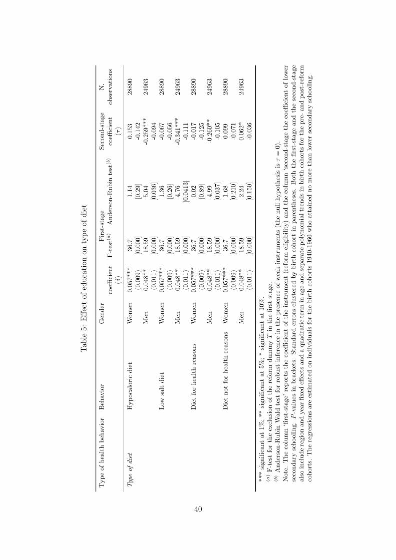
Tab

le5:

Eff

ect

ofed

uca

tion

onty

pe

ofdie

t

Typ

eof

hea

lth

beh

avio

rB

ehav

ior

Gen

der

Fir

st-s

tage

Sec

on

d-s

tage

N.

coeffi

cien

tF

-tes

t(a)

An

der

son

-Ru

bin

test

(b)

coeffi

cien

tob

serv

ati

on

s(δ

)(τ

)

Typeofdiet

Hyp

oca

lori

cd

iet

Wom

en0.0

57***

36.7

1.1

40.1

53

28890

(0.0

09)

[0.0

00]

[0.2

9]

-0.1

42

Men

0.0

48**

18.5

95.0

4-0

.259***

24963

(0.0

11)

[0.0

00]

[0.0

36]

-0.0

94

Low

salt

die

tW

om

en0.0

57***

36.7

1.3

6-0

.067

28890

(0.0

09)

[0.0

00]

[0.2

6]

-0.0

56

Men

0.0

48**

18.5

94.7

6-0

.341***

24963

(0.0

11)

[0.0

00]

[0.0

413]

-0.1

11

Die

tfo

rh

ealt

hre

ason

sW

om

en0.0

57***

36.7

0.0

2-0

.017

28890

(0.0

09)

[0.0

00]

[0.8

9]

-0.1

25

Men

0.0

48**

18.5

94.9

9-0

.260**

24963

(0.0

11)

[0.0

00]

[0.0

37]

-0.1

05

Die

tn

otfo

rh

ealt

hre

ason

sW

om

en0.0

57***

36.7

1.6

80.0

99

28890

(0.0

09)

[0.0

00]

[0.2

10]

-0.0

71

Men

0.0

48**

18.5

92.2

40.0

62*

24963

(0.0

11)

[0.0

00]

[0.1

50]

-0.0

36

***

sign

ifica

nt

at1%

;**

sign

ifica

nt

at5%

;*

sign

ifica

nt

at

10%

.(a

)F

-tes

tfo

rth

eex

clu

sion

ofth

ere

form

du

mm

yT

inth

efi

rst

stage.

(b)

An

der

son

-Ru

bin

Wal

dte

stfo

rro

bu

stin

fere

nce

inth

ep

rese

nce

of

wea

kin

stru

men

ts(t

he

nu

llhyp

oth

esis

isτ

=0).

Not

e.T

he

colu

mn

‘firs

t-st

age’

rep

orts

the

coeffi

cien

tof

the

inst

rum

ent

(ref

orm

elig

ibil

ity)

an

dth

eco

lum

n‘s

econ

d-s

tage

the

coeffi

cien

tof

low

erse

con

dar

ysc

hool

ing.P

-val

ues

inb

rack

ets.

Sta

nd

ard

erro

rscl

ust

ered

by

bir

thco

hort

inp

are

nth

eses

.B

oth

the

firs

t-st

age

an

dth

ese

con

d-s

tage

also

incl

ud

ere

gion

and

year

fixed

effec

tsan

da

qu

ad

rati

cte

rmin

age

an

dse

para

tep

oly

nom

ialtr

end

sin

bir

thco

hort

sfo

rth

ep

re-

an

dp

ost

-ref

orm

coh

orts

.T

he

regr

essi

ons

are

esti

mat

edon

ind

ivid

uals

for

the

bir

thco

hort

s1940-1

960

wh

oatt

ain

edn

om

ore

than

low

erse

con

dary

sch

ooli

ng.

40

Tab

le6:

Eff

ect

ofed

uca

tion

onpre

venti

ve-c

are

beh

avio

rs

Typ

eof

hea

lth

beh

avio

rB

ehav

ior

Gen

der

Fir

st-s

tage

Sec

on

d-s

tage

N.

coeffi

cien

tF

-tes

t(a)

An

der

son

-Ru

bin

test

(b)

coeffi

cien

tob

serv

ati

on

s(δ

)(τ

)

Preventive-care

behavior

Mam

mog

ram

Wom

en0.0

57***

37.4

52.8

8-0

.342*

28,8

83

(0.0

09)

[0.0

00]

[0.1

1]

(0.1

89)

Pap

smea

rte

stW

om

en0.0

57***

36.3

70.2

8-0

.109

28,8

77

(0.0

09)

[0.0

00]

[0.6

0]

(0.1

95)

CB

MW

om

en0.0

40**

7.1

24.7

4-0

.850*

11,8

12

(0.0

15)

[0.0

15]

[0.0

4]

(0.4

40)

Gly

cem

iach

eck

last

year

Wom

en0.0

56***

24.5

31.6

1-0

.438

24,9

92

(0.0

11)

[0.0

00]

[0.2

2]

(0.3

68)

Men

0.0

49***

25.8

611.1

50.4

10***

22,0

72

(0.0

09)

[0.0

00]

[0.0

0]

(0.1

24)

Ch

oles

tero

lch

eck

last

year

Wom

en0.0

56***

24.5

32.8

2-0

.572

24,9

92

(0.0

11)

[0.0

00]

[0.1

1]

(0.3

80)

Men

0.0

49***

25.8

623.1

70.4

46***

22,0

72

(0.0

09)

[0.0

00]

[0.0

0]

(0.1

11)

Blo

od

pre

ssu

rech

eck

last

yea

rW

om

en0.0

56***

24.5

31.9

9-0

.398

24,9

92

(0.0

11)

[0.0

00]

[0.1

7]

(0.3

15)

Men

0.0

49***

25.8

62.2

00.2

27

22,0

72

(0.0

09)

[0.0

00]

[0.1

5]

(0.1

40)

N.

med

ical

exam

inat

ion

sw

ith

ou

tsy

mp

tom

sW

om

en0.0

56***

24.5

33.0

9-0

.195

24,9

92

(0.0

11)

[0.0

00]

[0.0

9]

(0.1

21)

Men

0.0

49***

25.8

60.0

20.0

18

22,0

72

(0.0

09)

[0.0

00]

[0.8

9]

(0.1

28)

N.

pai

dex

amin

atio

ns

Wom

en0.0

56***

24.5

30.3

1-0

.113

24,9

92

(0.0

11)

[0.0

00]

[0.5

9]

(0.1

89)

Men

0.0

49***

25.8

61.9

5-0

.273

22,0

72

(0.0

09)

[0.0

00]

[0.1

8]

(0.1

66)

Flu

shot

Wom

en0.0

56***

24.5

30.4

5-0

.070

24,9

92

[0.0

11]

[0.0

00]

[0.5

1]

(0.1

00)

Men

0.0

49***

25.8

60.3

40.0

96

22,0

72

(0.0

09)

[0.0

00]

[0.5

7]

(0.1

64)

***

sign

ifica

nt

at1%

;**

sign

ifica

nt

at5%

;*

sign

ifica

nt

at

10%

.(a

)F

-tes

tfo

rth

eex

clu

sion

ofth

ere

form

du

mm

yT

inth

efi

rst

stage.

(b)

An

der

son

-Ru

bin

Wal

dte

stfo

rro

bu

stin

fere

nce

inth

ep

rese

nce

of

wea

kin

stru

men

ts(t

he

nu

llhyp

oth

esis

isτ

=0).

Not

e.T

he

colu

mn

‘firs

t-st

age’

rep

orts

the

coeffi

cien

tof

the

inst

rum

ent

(ref

orm

elig

ibil

ity)

an

dth

eco

lum

n‘s

econ

d-s

tage

the

coeffi

cien

tof

low

erse

con

dary

sch

ooli

ng.

P-v

alu

esin

bra

cket

s.S

tan

dar

der

rors

clu

ster

edby

bir

thco

hort

inp

are

nth

eses

.B

oth

the

firs

t-st

age

an

dth

ese

con

d-s

tage

als

oin

clu

de

regio

nan

dye

ar

fixed

effec

tsan

da

qu

adra

tic

term

inag

ean

dse

par

ate

pol

yn

om

ial

tren

ds

inb

irth

coh

ort

sfo

rth

ep

re-

an

dp

ost

-ref

orm

coh

ort

s.T

he

regre

ssio

ns

are

esti

mate

don

ind

ivid

uals

for

the

bir

thco

hor

ts19

40-1

960

wh

oat

tain

edn

om

ore

than

low

erse

con

dary

sch

ooli

ng.

41

Tab

le7:

Pot

enti

alpat

hw

ays

for

the

effec

tof

educa

tion

onhea

lth

Dep

end

ent

vari

able

Gen

der

Fir

st-s

tage

Sec

on

d-s

tage

N.

coeffi

cien

tF

-tes

t(a)

An

der

son

-Ru

bin

test

(b)

coeffi

cien

tob

serv

ati

on

s(δ

)(τ

)

Lab

our

forc

ep

arti

cip

atio

nW

omen

0.0

58***

37.1

95.3

50.5

20**

28922

(0.0

09)

[0.0

0]

[0.0

3]

(0.2

10)

Men

0.0

41***

16.0

315.8

31.9

51***

24985

(0.0

10)

[0.0

0]

[0.0

0]

(0.6

36)

Physi

cal

inte

nsi

tyof

hou

sew

ork

and

job

Wom

en0.0

56***

24.5

32.2

30.9

11*

24992

(0.0

11)

[0.0

0]

[0.1

5]

(0.5

52)

Men

0.0

47***

27.3

811.9

44.6

60***

22072

(0.0

09)

[0.0

0]

[0.0

0]

(1.7

09)

Any

hig

hin

ten

sity

physi

cal

acti

vit

yW

omen

0.0

56***

24.5

30.5

30.0

96

24992

(hou

sew

ork,

job,

physi

cal

exer

cise

)(0

.011)

[0.0

0]

[0.4

7]

(0.1

27)

Men

0.0

47***

27.3

82.3

00.4

96

22072

(0.0

09)

[0.0

0]

[0.1

4]

(0.3

62)

Em

otio

nal

pro

ble

ms

Wom

en0.0

56***

24.5

30.7

00.1

49

24992

(0.0

11)

[0.0

0]

[0.4

1]

(0.1

77)

Men

0.0

47***

27.3

81.1

30.1

81

22072

(0.0

09)

[0.0

0]

[0.3

0]

(0.1

71)

Mar

ital

stat

us

Wom

en0.0

58***

37.1

91.2

8-0

.074

28922

(0.0

09)

[0.0

0]

[0.2

7]

(0.0

68)

Men

0.0

41***

16.0

31.5

9-0

.112

24985

(0.0

10)

[0.0

0]

[0.2

2]

(0.0

75)

***

sign

ifica

nt

at1%

;**

sign

ifica

nt

at5%

;*

sign

ifica

nt

at

10%

.(a

)F

-tes

tfo

rth

eex

clu

sion

ofth

ere

form

du

mm

yT

inth

efi

rst

stage.

(b)

An

der

son

-Ru

bin

Wal

dte

stfo

rro

bu

stin

fere

nce

inth

ep

rese

nce

of

wea

kin

stru

men

ts(t

he

nu

llhyp

oth

esis

isτ

=0).

Not

e.E

ach

row

rep

rese

nts

the

resu

ltof

ase

par

ate

regre

ssio

nu

sin

gth

ed

epen

den

tva

riab

les

list

edin

the

firs

tco

lum

n,

an

des

tim

ate

du

sin

ga

FR

D.

Th

eco

lum

n‘fi

rst-

stag

e’re

por

tsth

eco

effici

ent

of

the

inst

rum

ent

(ref

orm

elig

ibil

ity)

an

dth

eco

lum

n‘s

econ

d-s

tage

the

coeffi

cien

tof

low

erse

con

dar

ysc

hool

ing.P

-valu

esin

bra

cket

s.S

tan

dard

erro

rscl

ust

ered

by

bir

thco

hort

inp

are

nth

eses

.B

oth

the

firs

t-st

age

and

the

seco

nd

-sta

geal

soin

clu

de

regio

nan

dyea

rfi

xed

effec

tsan

da

qu

ad

rati

cte

rmin

age

an

dse

para

tep

oly

nom

ial

tren

ds

inb

irth

coh

orts

for

the

pre

-an

dp

ost-

refo

rmco

hort

san

dare

esti

mate

don

ind

ivid

uals

for

the

bir

thco

hort

s1940-1

960

wh

oat

tain

edn

om

ore

than

low

erse

con

dar

ysc

hool

ing.

42

Table 8: Statistical associations between selected variables

Main independent Gender coefficient R2 N.variable observations

Dependent variable is BMILabour force participation Women -0.295*** 0.050 28896

(0.057)Men -0.084 0.018 24965

(0.065)Physical intensity of housework and job Women -0.044 0.048 24992

(0.028)Men -0.035 0.016 22072

(0.017)Married Women 0.642*** 0.051 28896

(0.132)Men 0.376*** 0.019 24965

(0.067)Emotional problems Women 0.592*** 0.051 24992

(0.061)Men -0.102 0.016 22072

(0.075)Pregnancy weight gain more than 15 Kg. Women 0.105 0.040 4753

(0.177)Dependent variable is pregnancy weight gainmore than 15 Kg.Lower secondary schooling Women 0.009 0.02 4753

(0.016)

*** significant at 1%; ** significant at 5%; * significant at 10%.

Note. Each row represents the result of a separate regression using the dependent variableslisted in the first column, and estimated using OLS. ‘Coefficients’ refer to the coefficientsof lower secondary schooling in each regression. Standard errors clustered by birth cohortin parentheses. All specifications also include region and year fixed effects and a quadraticterm in age and separate polynomial trends in birth cohorts for the pre- and post-reformcohorts and are estimated on individuals for the birth cohorts 1940-1960 who attained nomore than lower secondary schooling.

43

Table A1. Descriptive statistics for women

Variable Obs Mean Std. Dev. Min Max

Body Mass Index (BMI) 28896 25.435 4.235 12.05 52.07Overweightness 28896 0.475 0.499 0 1Obesity 28896 0.141 0.348 0 1Chronic illness (self-reported) 28922 0.488 0.500 0 1Chronic illness (diagnosed) 28922 0.443 0.497 0 1Days with limitations (last 4 weeks) 28922 1.648 5.267 0 28Days in bed (last 4 weeks) 28922 0.501 2.371 0 28Smoking 24992 0.189 0.391 0 1Ever smoker 24992 0.327 0.469 0 1Intense physical activity 24992 0.028 0.165 0 1Regular physical activity 24992 0.156 0.363 0 1Any continuous physical activity 24992 0.514 0.500 0 1Dietary regime 28890 0.146 0.353 0 1Hypocaloric diet 28890 0.099 0.299 0 1Low salt diet 28890 0.058 0.234 0 1Diet for health reasons 28890 0.114 0.318 0 1Diet for non health reasons 28890 0.031 0.174 0 1Mammogram 28883 0.558 0.497 0 1Pap smear test 28877 0.697 0.460 0 1CBM 11812 0.336 0.472 0 1Glycemia check last year 24992 0.546 0.498 0 1Cholesterol check last year 24992 0.541 0.498 0 1Blood pressure check last year 24992 0.640 0.480 0 1N. medical examinations without symptom 24992 0.088 0.283 0 1N. paid examinations 24992 0.173 0.616 0 14Flu shot 24992 0.134 0.341 0 1

44

Table A2. Descriptive statistics for men

Variable Obs Mean Std. Dev. Min Max

Body Mass Index (BMI) 24965 26.631 3.455 12.79 55.56Overweightness 24965 0.661 0.474 0 1Obesity 24965 0.155 0.362 0 1Chronic illness (self-reported) 24985 0.409 0.492 0 1Chronic illness (diagnosed) 24985 0.369 0.483 0 1Days with limitations (last 4 weeks) 24985 1.306 4.731 0 28Days in bed (last 4 weeks) 24985 0.431 2.219 0 28Smoking 22072 0.339 0.473 0 1Ever smoker 22072 0.683 0.465 0 1Intense physical activity 22072 0.055 0.229 0 1Regular physical activity 22072 0.212 0.409 0 1Dietary regime 24963 0.107 0.310 0 1Hypocaloric diet 24963 0.071 0.257 0 1Low salt diet 24963 0.046 0.209 0 1Diet for health reasons 24963 0.091 0.287 0 1Diet for non health reasons 24963 0.017 0.128 0 1Glycemia check last year 22072 0.520 0.500 0 1Cholesterol check last year 22072 0.516 0.500 0 1Blood pressure check last year 22072 0.604 0.489 0 1Any continuous physical activity 22072 0.557 0.497 0 1N. medical examinations without symptom 22072 0.062 0.241 0 1N. paid examinations 22072 0.122 0.538 0 13Flu shot 22072 0.121 0.326 0 1

45

Table A3. OLS estimates for women

Dependent variable Coeff. St.err. Observations R-squared

BMI -1.071*** (0.068) 28,896 0.062Overweightness -0.113*** (0.007) 28,896 0.052Obesity -0.060*** (0.005) 28,896 0.019Chronic illness (self-reported) -0.035*** (0.006) 28,922 0.124Chronic illness (diagnosed) -0.039*** (0.007) 28,922 0.172Days with limitations (last 4 weeks) -0.156** (0.069) 28,922 0.008Days in bed (last 4 weeks) -0.039 (0.027) 28,922 0.005Smoking 0.044*** (0.006) 24,992 0.038Ever smoker 0.088*** (0.007) 24,992 0.063Intense physical activity 0.018*** (0.002) 24,992 0.015Regular physical activity 0.035*** (0.004) 24,992 0.066Any continuous physical activity 0.071*** (0.006) 24,992 0.122Dietary regime -0.001 (0.005) 28,890 0.020Hypocaloric diet -0.002 (0.005) 28,890 0.047Low salt diet -0.005 (0.003) 28,890 0.051Diet for health reasons -0.009 (0.005) 28,890 0.033Diet for non health reasons 0.008** (0.003) 28,890 0.005Mammogram 0.049*** (0.006) 28,883 0.134Pap smear test 0.059*** (0.005) 28,877 0.110CBM 0.029*** (0.010) 11,812 0.097Glycemia check last year 0.016** (0.007) 24,992 0.052Cholesterol check last year 0.015** (0.007) 24,992 0.055Blood pressure check last year 0.012* (0.006) 24,992 0.077N. medical examinations without symptom 0.006 (0.004) 24,992 0.003N. paid examinations 0.025** (0.010) 24,992 0.002Flu shot -0.002 (0.006) 24,992 0.073

*** significant at 1%; ** significant at 5%; * significant at 10%.

Note. Each row represents the result of a separate regression using the dependent variableslisted in the first column, and estimated using OLS. ‘Coefficients’ refer to the coefficients oflower secondary schooling in each regression. Standard errors clustered by birth cohort inparentheses. All specifications also include region and year fixed effects and a quadratic termin age and separate polynomial trends in birth cohorts for the pre- and post-reform cohortsand are estimated on individuals for the birth cohorts 1940-1960 who attained no more thanlower secondary schooling.

46

Table A4. OLS estimates for men

Dependent variable Coeff. St.err. Observations R-squared

BMI -0.211 (0.040) 24,965 0.019Overweightness -0.011** (0.005) 24,965 0.016Obesity -0.030*** (0.003) 24,965 0.010Chronic illness (self-reported) -0.011 (0.007) 24,985 0.077Chronic illness (diagnosed) -0.010 (0.007) 24,985 0.116Days with limitations (last 4 weeks) -0.207 (0.086) 24,985 0.004Days in bed (last 4 weeks) -0.121*** (0.039) 24,985 0.004Smoking -0.011 (0.008) 22,072 0.028Ever smoker 0.012** (0.005) 22,072 0.005Intense physical activity -0.002 (0.005) 22,072 0.022Regular physical activity 0.036*** (0.004) 22,072 0.021Any continuous physical activity 0.041*** (0.007) 22,072 0.061Dietary regime 0.078*** (0.008) 24,963 0.095Hypocaloric diet -0.000 (0.004) 24,963 0.042Low salt diet -0.003 (0.003) 24,963 0.037Diet for health reasons -0.005 (0.005) 24,963 0.030Diet for non health reasons 0.003** (0.001) 24,963 0.005Glycemia check last year 0.034*** (0.006) 22,072 0.041Cholesterol check last year 0.034*** (0.006) 22,072 0.041Blood pressure check last year 0.035*** (0.007) 22,072 0.060N. medical examinations without symptom 0.006** (0.002) 22,072 0.007N. paid examinations 0.034*** (0.008) 22,072 0.004Flu shot -0.003 (0.004) 22,072 0.056

*** significant at 1%; ** significant at 5%; * significant at 10%.

Note. Each row represents the result of a separate regression using the dependent variableslisted in the first column, and estimated using OLS. ‘Coefficients’ refer to the coefficients oflower secondary schooling in each regression. Standard errors clustered by birth cohort inparentheses. All specifications also include region and year fixed effects and a quadratic termin age and separate polynomial trends in birth cohorts for the pre- and post-reform cohortsand are estimated on individuals for the birth cohorts 1940-1960 who attained no more thanlower secondary schooling.

47