the effect of physical and cognitive decline at older ages

NBER WORKING PAPER SERIES

THE EFFECT OF PHYSICAL AND COGNITIVE DECLINE AT OLDER AGES ONJOB MISMATCH AND RETIREMENT

Péter HudomietMichael D. Hurd

Susann RohwedderRobert J. Willis

Working Paper 25229http://www.nber.org/papers/w25229

NATIONAL BUREAU OF ECONOMIC RESEARCH1050 Massachusetts Avenue

Cambridge, MA 02138November 2018

Support from the University of Michigan Retirement Research Center Award RRC08098401-09 is gratefully acknowledged. The views expressed herein are those of the authors and do not necessarily reflect the views of the National Bureau of Economic Research.

NBER working papers are circulated for discussion and comment purposes. They have not been peer-reviewed or been subject to the review by the NBER Board of Directors that accompanies official NBER publications.

© 2018 by Péter Hudomiet, Michael D. Hurd, Susann Rohwedder, and Robert J. Willis. All rights reserved. Short sections of text, not to exceed two paragraphs, may be quoted without explicit permission provided that full credit, including © notice, is given to the source.

The Effect of Physical and Cognitive Decline at Older Ages on Job Mismatch and RetirementPéter Hudomiet, Michael D. Hurd, Susann Rohwedder, and Robert J. WillisNBER Working Paper No. 25229November 2018JEL No. J26,J81

ABSTRACT

Physical and cognitive abilities of older workers decline with age, which can cause a mismatch between abilities and job demands, potentially leading to early retirement. We link longitudinal Health and Retirement Study data to O*NET occupational characteristics to estimate to what extent changes in workers’ physical and cognitive resources change their work-limiting health problems, mental health, subjective probabilities of retirement, and labor market status. While we find that physical and cognitive decline strongly predict all outcomes, only the interaction between large-muscle resources and job demands is statistically significant, implying a strong mismatch at older ages in jobs requiring large-muscle strength. The effects of declines in fine motor skills and cognition are not statistically different across differing occupational job demands.

Péter HudomietRAND Corporation1776 Main StreetSanta Monica, CA 90407Email: [email protected]@rand.org

Michael D. HurdRAND Corporation1776 Main StreetSanta Monica, CA 90407and [email protected]

Susann RohwedderRAND1776 Main StreetP.O. Box 2138Santa Monica, CA [email protected]

Robert J. Willis3254 ISRUniversity of MichiganP. O. Box 1248426 Thompson StreetAnn Arbor, MI 48106and [email protected]

1

Introduction

Poor health is one of the strongest drivers of early retirement (Blundell, Britton, Costa Dias,

and French, 2017; Cahill, Giandrea, and Quinn 2006; Fisher, Chaffee, and Sonnega 2016;

McGarry 2004; Rice et al. 2011; van Rijn et al. 2014) and it reduces the likelihood of continuing

work after separation from career jobs (Topa et al. 2009). Poor health or declining cognitive ability

makes it more burdensome to carry out job tasks, and the magnitude of the added burden depends

on job characteristics. For example, someone with minor back pain may have little difficulty

carrying out the tasks of an office clerk but may be unable to carry heavy objects, a task frequently

performed by construction workers. Conversely, an accountant whose memory starts to deteriorate

may have more trouble performing well on the job compared to a hairdresser with early-stage

memory decline.

When workers’ capabilities become mismatched with the demands of their jobs, there are

several ways to adjust, but changes in their work status are more likely to occur. For example,

workers may initially stay in their current job positions and increase their level of effort to

compensate for their decline in cognitive and physical resources. This greater effort, however,

may lead to dissatisfaction with work, exhaustion, and (mental) health problems. Alternatively,

employers may accommodate the changing capabilities of their aging employees. Workers may

also reduce their work hours to compensate for their increased difficulty working, or switch to

different jobs or tasks better suited to their changing abilities, either in the same or in a less-

demanding occupation. In most scenarios workers will likely leave the labor force earlier than

they would have in the absence of physical or cognitive decline.

Understanding how mismatch between individuals’ resources and job demands affects

labor force participation at older ages is important because early retirement may leave

2

individuals and their families financially vulnerable at older ages. To the extent that better

accommodation of mismatch allows individuals to work longer it will not only improve their

own financial security, but it would also relieve financial pressures on public programs such as

Social Security or Medicare. Even if employers wanted to accommodate work limitations, the

mismatch between the worker’s abilities and the job demands may eventually become too large,

resulting in job separation. Policymakers need to understand how often this happens: such

mismatches and separations may prevent workers from working to the ages they desire or had

planned on.

In this paper, we study how age-related mismatch between job demands and workers’

health and cognitive abilities affects retirement outcomes. We use longitudinal data from the

Health and Retirement Study (HRS) linked to detailed occupational characteristics from the

O*NET project.2 We considered a large set of outcomes that signaled mismatch, but focus on

five of them in this study: work-limiting health problems, depressive symptoms, the subjective

probability of working full time after age 65, transition probabilities from work to retirement,

and transitions to disability.

When possible, we use panel econometric models to estimate how changes in

individuals’ resources and the interactions between resources and job demands affect changes in

these outcome variables. These empirical models control for individuals’ initial conditions and

hence are more credible than models relying on cross-sectional variation.

We consider mismatch in two physical and two cognitive domains. Regarding physical

domains, we use measures from the HRS of deficits in individuals’ resources or capabilities:

2 The O*NET database (www.onetcenter.org) contains information on hundreds of standardized and occupation-specific descriptors that capture, among other things, the characteristics and requirements of the jobs, including the intensity of various activities involved in doing a particular job.

http://www.onetcenter.org/

3

whether they have large muscle problems such as having difficulties with stooping, kneeling, or

crouching, or with pushing or pulling large objects; or whether they have fine motor skill

problems such as having difficulties with picking up a dime from a table and dressing. Regarding

cognitive domains, we use a 27-point working and episodic memory score from the HRS, which

is closely linked to fluid intelligence and decision-making abilities (Del Missier et al. 2013).

We pair these resource measures with data on detailed job demands from the O*NET

project. The O*NET, sponsored by the U.S. Department of Labor’s Employment and Training

Administration, is based on a combination of surveys, expert assessments, and tests. The ratings

are available for occupations identified by three-digit codes that can be linked to occupations of

HRS respondents.

We use four O*NET job-demand measures: First, we use measures on dynamic strength,

i.e., the ability to exert muscle force repeatedly or continuously. We paired these with the HRS

large-muscle resource measure. Second, we use measures on finger dexterity, i.e., the ability to

make precisely coordinated movements of the fingers. We pair these with the HRS fine-motor

skill resource measure. Third, we use measures on memorization, i.e., the ability to remember

information. We pair these with the HRS cognition-resource measure. Fourth, we use O*NET

measures on analyzing data or information, also pairing them with the HRS cognition-resource

measure.

We found that, among HRS respondents, large-muscle strength, fine-motor skills, and

cognitive abilities significantly and strongly decline with age. Furthermore, these declines lead to

higher reports of work-limiting health problems, more depressive symptoms, lower subjective

probabilities of working full-time past age 65, and more transitions from full-time work to

retirement and disability.

4

To capture the degree of job mismatch for respondents, we use terms capturing the

interaction between resource decline and job demands.3 Such terms, for example, show whether

cognitive decline reduces the ability to work in all jobs or only in cognitively demanding ones.

We found only one statistically significant interaction term: that for large muscle problems.

Workers who develop large-muscle limitations are more likely to report changes in most

outcomes when they work in occupations that rely heavily on physical strength than when they

work in occupations that do not rely on physical strength. The interaction effects were large and

statistically significant for work-limiting health problems, mental health, subjective work

expectations, and transitions to disability. In contrast to the large muscle results, the interaction

terms of workers’ resources and job demands for fine motor skills and for cognition were not

statistically significant, suggesting that declines in workers’ fine motor skills or cognition did not

lead to significant differences in their outcomes by occupational job demands.

Our preferred statistical models use panel variation for identification rather than cross-

sectional variation. But, because our data are observational, we discuss threats to identification,

including omitted factors, selection, and reverse causality, and we estimate alternative

specifications and tests. For example, we estimate models with alternative sets of controls, we

estimate models on different samples, and we estimate placebo regressions on lagged values of

the outcome variables. These results support a causal interpretation, perhaps because within-

person changes in the resources (health) are relatively random events in this age range.

3 The term “mismatch” has been used in the economics literature to describe different issues, such as the misalignment of the demand and supply of skills in countries or regions (Cappelli 2015); or the difference between students’ abilities and the qualities of their schools (Dillon and Smith, 2017). We, instead, define it based on workers’ resources and the demands of their current jobs.

5

It is important to point out, however, that finding a significant causal effect (or absence of

effect) does not necessarily reveal much about the mechanisms linking changes in resources to

labor market outcomes. When an exogenous change in a worker’s health or capabilities occurs

that reduces productivity or increases the disutility of work, the consequences of that change may

lead to responses by the employer or the employee to offset these effects through medical

treatment, equipment, changes in hours, organization of work, task assignments and so on. A

significant causal effect of an exogenous change in resources on retirement outcomes depends on

whether the present value of pecuniary and non-pecuniary costs to the employer and employee of

offsetting adjustments are smaller than the net benefits to both parties of continued employment.

Heterogeneity in task demands and skill supplies across firms and workers due to variation in

firm technology and worker skills and preferences4 is likely to lead to considerable heterogeneity

in the net costs of mismatch both within and across occupations and, therefore, to considerable

unmeasured variation in the effects of exogenous changes in worker resources on retirement

outcomes. In this paper, we estimate the average causal effect of mismatch for workers in the

equilibrium match. The plausibly large variance in the magnitude of effects implies that there is

considerable room for general equilibrium effects of policy changes that are not captured by our

analysis. However, we believe that our analysis of mismatch helps distinguish types of workers

and occupations for which private or public interventions to overcome mismatch are likely to be

helpful.

Our work builds on several previous strands of research. Several studies have shown the

role of occupational characteristics in explaining job polarization, wage inequality, and career

decisions (Acemoglu and Autor 2011; Autor, Levy, and Murnane 2003; James 2011; Yamaguchi

4 See Lindenlaub (2017) for outcomes of equilibrium sorting on multiple dimensions in the labor market.

6

2012, 2018), and a smaller number of papers explored the role of occupational characteristics in

the retirement process (Angrisiani, Kapteyn, and Meijer 2015; Bowlus, Mori, and Robinson,

2016; Belbase, Sanzenbacher, and Gillis 2016; Sonnega et al. 2018).

The study of Belbase et al. (2016) is most closely related to ours. It showed that

individuals in occupations that heavily rely on skills that tend to decline with age are more likely

to retire earlier. Nevertheless, our work differs from theirs in several ways. First, we identified

four dimensions of job characteristics for which the HRS elicits respondents’ abilities: two

cognitive and two physical. Second, in addition to analyzing the role of job demands in the

timing of retirement we analyzed the role of respondents’ corresponding abilities at the

individual level and changes therein, which is an important but often neglected heterogeneity

(Bowlus et al., 2016). Third, and maybe most importantly, we analyzed the interaction between

abilities and job demands, whereas Belbase et al. (2016) did not use reports about workers’

abilities. Fourth, we used retirement expectations data, allowing us to observe the immediate

impact of changes in abilities and job mismatch. This has the further advantages of increased

sample size and panel variation for identification.

Other related research in psychology explores the person-environment fit. Wang and

Shultz (2010) suggested that the match between various aspects of the persons (workers) and

their work environment may affect work and retirement outcomes, including well-being and

retirement timing. Liebermann, Wegge, and Muller (2013) used a person-environment

framework in a study of German insurance workers to explore several hypotheses related to

workers’ expectations of remaining in the same job until retirement. McGonagle, et al. (2015)

investigate how the match between job demands, job resources and “perceived work ability”

affects work-related stress and work outcomes. Sonnega et al. (2018) compared objective

7

(O*NET) and subjective (HRS) job-demand measures and how they interacted with HRS

resource measures to predict retirement timing. We use a broader set of variables, and we use

panel econometric models that are less restrictive than cross-sectional models.

In the next section, we describe the HRS and O*NET data we analyze. We then present

separate sections on our methods and results. The final section presents our conclusions and a

discussion of the implications and limitations of our work.

2. Data

The HRS is the primary U.S. data source for studying the retirement process.5 It has a large

sample—approximately 20,000 responses per wave—of persons at least 50 years of age, and very

detailed panel information on them, including information about work, health, cognitive abilities,

and socioeconomic status. The HRS has interviewed respondents biennially since 1992.

2.1. Measurement of physical and cognitive resources

The HRS has very detailed information about individuals’ health, limitations in the

activities of daily living (ADLs), and cognitive abilities. We use three summary measures, created

by the RAND-HRS (2016),6 in this project. Table 1 provides an overview.

The first measure is termed “large-muscle problems” and represents difficulties with mild-

to-moderate physical activities. The measure comprises four items, each corresponding to the

respondent’s mention of any difficulty with:

1. sitting for about two hours

5 The HRS (Health and Retirement Study) is sponsored by the National Institute on Aging (grant number NIA U01AG009740) and is conducted by the University of Michigan: http://hrsonline.isr.umich.edu/ 6 The RAND HRS Data file is an easy to use longitudinal data set based on the HRS data. It was developed at RAND with funding from the National Institute on Aging and the Social Security Administration www.rand.org/labor/aging/dataprod/hrs-data.html.

http://www.rand.org/labor/aging/dataprod/hrs-data.html

8

2. getting up from a chair after sitting for long periods

3. stooping, kneeling, or crouching

4. pulling or pushing large objects like a living room chair.

The second measure is termed “fine motor problems” and it aims to capture problems with

the precise coordination of fingers, such as picking up small objects or buttoning a shirt

(Hoogendam et al. 2014). Our measure sums three items from the HRS about reporting difficulties

with:

1. dressing, including putting on shoes and socks

2. eating, including cutting food

3. picking up a dime from a table

The average value of this 0-3 score in our sample is only 0.047 (Table 2). Thus we

anticipate that this measure will not be very discriminatory, but it will distinguish people with

substantial problems (Carmeli, Patish, and Coleman 2003).

Our measure of cognitive ability is the 27-point scale of episodic memory (see Crimmins

et al. 2011), which is strongly related to fluid cognitive abilities (Del Missier et al. 2013). The

measure sums performance on four cognitive tests:

1. Immediate word recall of a list of 10 words (10 points)

2. Delayed word recall of the same list a few minutes later (10 points)

3. Serial subtraction of 7 from 100 five times (5 points)

4. Backward counting from 20 to 10 with two trials (2 points)

The physical measures are consistently available since 1994 for all interviews, including

interviews of proxy respondents for persons unwilling or unable to do the interview. The cognition

9

score is consistently available since 1996 but is not available in proxy interviews because cognitive

abilities can only be directly tested. All three resource measures are recoded so that higher values

represent more resources (better health). For the regression models we also standardized the

measures to have a zero mean and a standard deviation of one in our main analytic sample, which

comprises respondents 50 to 70 years of age who are working full-time.

2.2. Measurement of job demands

The HRS provides information on workers’ occupations by three-digit occupational codes

of the U.S. Census Bureau. The classification changed in 2006 from the 1980 to the 2000 census

classifications, but cross-walks are available between these specifications (Hudomiet 2015; Carr

et al. 2016). The detailed occupations are linked to detailed occupational characteristics from the

O*NET data, similarly to Belbase, Sanzenbacher, and Gillis (2016) and Carr et al. (2016). We

extract four key dimensions of job demands that are closely related to the resource measures. Table

1 provides an overview.

The dynamic strength dimension relates to individuals’ ability to exert muscle force

repeatedly or continuously over time. This involves muscular endurance and resistance to muscle

fatigue. Occupations that score the highest on this measure include fire fighters, masons and

construction workers; occupations that score lowest include management, engineering and

financial ones. We pair the dynamic strength measure with the HRS large-muscle resource

measure.

The finger dexterity dimension describes individuals’ ability to make precisely coordinated

movements of the fingers of one or both hands to grasp, manipulate, or assemble very small

objects. Occupations scoring highest on this measure include dentists, aircraft mechanics, data

entry keyers, and precision textile, apparel, and furnishings machine workers. Occupations scoring

10

lowest include real estate sales, management analysists, human resource clerks and clergy. We

pair this job-demand measure with the HRS fine-motor skill resource measure.

The memorization dimension describes individuals’ ability to remember information such

as words, numbers, pictures, and procedures. Occupations scoring highest on this measure include

clergy, primary school teachers, lawyers, bartenders, and waiters/waitresses. Occupations scoring

lowest include janitors, painters, vehicle washers, and textile sewing machine operators. We pair

this job-demand measure with the HRS cognition-resource measure.

The “analyzing data or information” dimension captures work activities of identifying the

underlying principles, reasons, or facts of information by breaking down information or data into

separate parts. Occupations scoring highest include management analysts and various science jobs;

occupations scoring lowest include mail carriers, vehicle washers, door-to-door sales, and laundry

workers. We also pair this job-demand measure with the HRS cognition-resource measure.

Appendix A.1. discusses details of defining the four job-demand measures based on the

detailed HRS occupation codes. The job-demand measures range from 0 to 1. In our regression

analyses we use standardized measures that have a mean of zero and standard deviation of 1.0

among 50 to 70 years old full-time workers.

2.3. The outcome variables

Our conceptual framework considers how an increasing mismatch between the resources of

workers and the demands of their jobs will influence a number of outcomes. We considered a

large set of outcome variables and chose the following for analysis:

11

• Self-reports of any impairment or health problem that limits the kind or amount of paid

work respondents can do. We expect that any mismatch between individuals’ resources

and the demands of their jobs would increase the report of such impairments.

• The number of depressive symptoms individuals have, using the eight-item HRS version

of the Center for Epidemiological Studies-Depression (CESD) Scale. We expect that any

mismatch between individuals’ resources and the demands of their jobs would increase

the number of depressive symptoms.

• Subjective expectations to work full-time after age 65 (or 62). The HRS asks

respondents, Thinking about work in general and not just your present job, what do you

think the chances are that you will be working full-time after you reach age 65 [or 62]?

This measure of expected future work is highly predictive of actual future work at age 65

or 62 (Hurd, 2009). We expect that a mismatch between a worker’s resources and job

demands decreases the subjective probabilities of working full-time in the future and so

will predict earlier retirement.

These outcome variables are available for both workers and non-workers. They are

therefore well-suited for panel econometric modeling. Depressive symptoms and subjective

expectations, however, are not collected in proxy interviews due to their subjective nature.

Missing outcome variables were typically ignored in our analysis, except for subjective

expectations. Beginning in 2006, the HRS asked all respondents their subjective probabilities of

working full-time after age 62 and 65. Prior to 2006, however, non-working individuals were only

asked about the probabilities that they would ever work in the future, resulting in partial responses

to P65: a 0% answer about any work in the future implies a 0% chance of working full-time after

ages 62 or 65. Those, who provided a non-zero answer before 2006, however, were not asked

12

about full-time work after ages 62 and 65. These observations were imputed using a regression-

based imputation model with many predictors including lagged values of these variables. See

Appendix A.2. for details.

We also analyze wave-to-wave transition probabilities from full-time work to either full-

retirement or disability. The labor force status variables are based on the RAND-HRS (2016)

definitions. We expected that mismatch between worker resources and job demands would

increase the transition probability from work to retirement or disability status. Because actual

transitions between these states are infrequent, with many workers experiencing just one

transition, panel statistical methods are not well suited for their analysis, so we have to use other,

more restrictive methods.

We also analyze the effect of mismatch between worker resources and job demands on

the probabilities of a worker switching employers between HRS waves, the enjoyment

individuals derive from work, and the likelihood an individual will seek another job while

working.

2.4. Other variables

Other variables we use in our analysis are

• Age

• Gender

• Race (white, black, other)

• Education (high-school dropout, high school graduate, college dropout, college graduate)

• Marital status (married or not)

• Whether one’s spouse works

13

• Whether individuals have DB or DC pension plans

• Whether individuals are covered by health insurance either by their own or their spouse’s

employers.

• Self-employment status

• Job tenure

• Total household income

• Total household wealth, excluding employer-based retirement wealth7 (such as 401k

balances or defined benefit plan entitlements) and value of secondary residence8

We use the RAND-HRS dataset for these variables. Total household income and total

household wealth were imputed in case of missing information by the RAND team as explained

by RAND-HRS (2016). In a handful of cases some control variables (such as education) were also

missing. As discussed in Appendix A.2. missing controls were replaced by the modes of the

variables. Missing outcome variables or explanatory variables (other than the subjective

expectations discussed above), however, were not imputed.

2.5. The sample

We restrict our sample in several ways. We use the 1994-2014 waves of the HRS,

excluding the 1992 data because many variables of interest to this study were missing in that

wave. We also limit our analysis sample to person-year observations when individuals were

7 Information about employer sponsored pensions is collected by HRS for all current and previous employers (although limited to jobs held for 5 years or more for employment prior to the first HRS interview). Measurement error on pension plan type, changes in survey design across waves and the large number of components involved makes the derivation of pension wealth measures a major and complicated undertaking, with considerable ambiguity in the profession how best to accomplish this task. 8 HRS did not ask for the value of any secondary residence in the third wave (1996), so the total wealth measure we use excludes that.

14

between 50 and 70 years of age. Individuals with missing gender (only two person-year

observations) or occupations (322 person-year observations) are also excluded.

Some variables are not available in the 1994 wave or in proxy interviews (e.g., cognitive

abilities, expectations, CESD), so we exclude these from analyses where necessary.

Our main analyses are carried out on those who work full-time in one wave and are

observed in the succeeding wave, irrespective of labor force status in the next wave. In a few

cases, however, we do not restrict the sample based on current or future labor force statuses.

The HRS data comes with survey weights. Some individuals were initially interviewed

before they were age-eligible in which case they have a sample weight of zero. To maximize

information about initial job matches we report unweighted results.9 Weighted results are very

similar, probably because our panel econometric models are little affected by weights that (mostly)

correct for stratified sampling.

Table 2 presents descriptive information about our unweighted sample, including 50-70-

year-old full-time workers (not restricted by future labor force status). Altogether we have about

47,000 person-year observations, but some variables are missing for various reasons discussed

earlier. About half of the sample is female, almost one-fourth is non-white, more than one-fourth

has a college degree, and nearly three-fourths is married. Most individuals in our sample have

only a few, if any, physical limitations, with less than one in ten reporting a health condition that

limits working. On average, they report having one (of eight queried) depressive symptoms.

Appendix A.3. includes a table with weighted statistics that are very similar.

9 The HRS interviews spouses of age-eligible HRS respondents. Some spouses were not themselves age-eligible at their initial interview and so have an HRS weight of zero.

15

3. Methods

Suppose that as workers enter their early 50’s they are in job equilibrium: their physical

and cognitive capabilities are well matched to the demands of their job. Comparing responses

across individuals about job demands may reveal few mismatches because those workers most

suited to the demands will have sorted into those jobs. For example, strong men will have taken

up jobs that require considerable strength. If they are asked, however, whether the job requires

strength, they may not acknowledge the full extent of those demands. Because of such good

matches, there may be little relationship between anticipated retirement and job demands. Yet a

person of medium strength put into such a job would likely anticipate early retirement. Similarly,

as time passes the quality of the match may deteriorate even for a strong worker because of

decreases in physical health.

Our empirical strategy is based on the observation that because of health shocks or gradual

declines in physical and cognitive resources, jobs that were once a good match to a worker’s

characteristics may become increasingly mismatched.

3.1. Panel models

A strength of our approach is its use of panel data. By using panel-data methods, we can

control for initial conditions, in particular the initial quality of job matches. We illustrate our

empirical strategy with the example of the subjective probability of working past age 65, but

similar methods are used for the other outcomes.

We estimate the following model

(1) 65, 1 0 1 2 , 1 3 4 , 1 5 ,i t it i t it it i t it itp r r d d r Xβ β β β β β ε+ + +∆ = + + ∆ + + ×∆ + +

16

where 65itp is the subjective probability of working full time after age 65 for individual i at wave

t; itr denotes individuals’ resources, itd represents job demands; itX is a set of control variables

(such as changes in marital status, and interview wave indicators), itε is the error term; and ∆

indicates changes from wave t to wave t+1. The coefficients of interest are the interaction terms (

4β ).

We interpret the coefficients in (1) as the causal effect of resources (health) on the

outcomes by job demands. This specification is similar to a first-difference estimator, but the job

demands are fixed at the time t values so that changes in the right hand side variables only reflect

health rather than job changes. The model assumes a zero correlation between the error term in (1)

and changes in the HRS resources, as well as between the error and job demands and the interaction

terms.

The main threat to identification is omitted variable bias: that is, a left-out factor

simultaneously triggers changes in health and the outcomes. For example, a large inheritance may

allow people to quit their jobs and invest more in their health (Schwandt, 2018); or if employers

offer health insurance that may change workers’ health and labor supply. To explore the extent of

omitted variable bias we estimate models with different set of control variables as robustness

checks.

Another threat to identification is reverse causality: retirement itself may affect the physical

and mental health of individuals (Atalay and Barrett, 2014; Blundell, et al. (2017); Insler, 2014;

Mazzonna and Peracchi, 2016; Rohwedder and Willis, 2010). As a robustness check we restrict

the sample to full-time workers at both time t and t+1. These alternative estimates are likely biased

toward zero, because retirement is also a channel though which health shocks affect the outcome

17

variables. For these reasons, we interpret the estimates on this reduced sample as lower bounds of

the true effects.

A third threat to identification is selection into jobs: people in different jobs may have

different trajectories in their health and/or the outcome variables, but these differences may be

independent of their jobs. For example, blue collar workers may be a selected sample with faster

than average declines in health and labor supply. To explore this hypothesis, we estimated placebo

regressions on past values of the outcome variables. This is a form of balancing test à la Pei et al.

(2017). Our identification assumptions predict no effect on past outcomes, while the job selection

hypothesis predicts similar coefficients to the contemporaneous variable model.

3.2. Transition models

When modeling wave-to-wave transition probabilities, we use the same models as (1)

above, but we use transition indicators on the left side of the equation. The identification

assumptions are technically speaking the same as in the panel models. However, these models do

not difference out individual fixed effects in the transition probabilities, and thus, these models

rely on stronger identification assumptions than the panel models. We perform the same robustness

checks on these models as on the panel models when feasible.

4. Results

4.1: Descriptive patterns

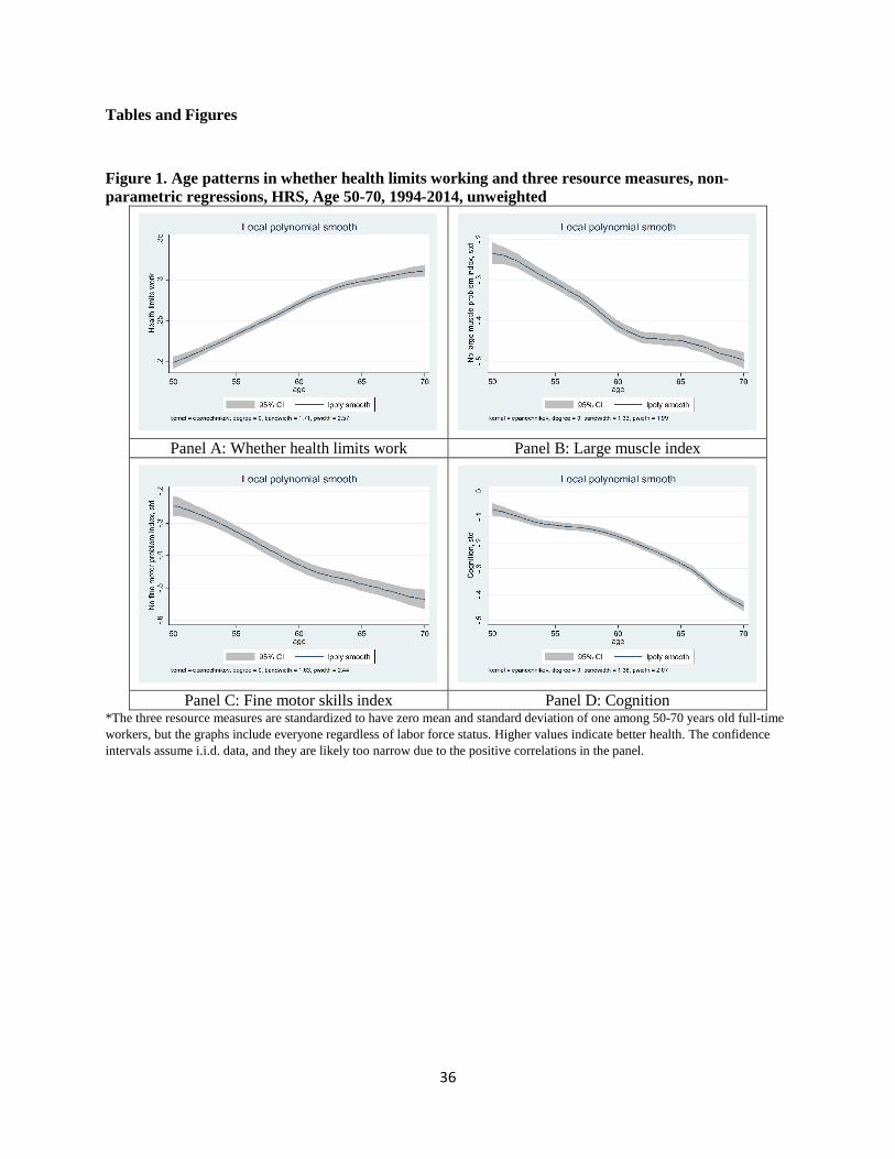
The four panels of Figure 1 show age patterns of work-limiting health problems and the

physical and cognitive resource measures for all HRS respondents 50 to 70 years of age. Our

theory predicts an increase in work-limiting health problems with age and a decrease in the three

resource measures.

18

Panel A indeed shows a sharp increase in the fraction reporting a work-limiting health

problem by age. The prevalence of such problems increases from about 20 percent among 50-

year-olds to more than 30% among 70-year-olds.

Panels B, C, and D show sharp declines in physical and cognitive resources. The

measures are standardized (zero mean and standard deviation of one) among 50-70-year old full-

time workers, but the graph includes everyone in that age range. All resource measures are

negative, on average, which indicates that full-time workers have more resources than the

general population at all ages between 50 and 70. We find a decrease of 0.25 standard deviations

in the large-muscle index among persons 50 to 70 years of age (Panel B), as well as a decline of

0.3 standard deviations in the fine-motor skills index (Panel C), and 0.4 standard deviations in

the cognition score (Panel D).

To get a sense of the quality of the pairings of HRS resources and O*NET job demands

pairs, Appendix A.4. shows correlations between these measures. We found large positive

correlations between cognitive ability and the two cognitive job demands which suggests that the

qualities of these pairs are good, and individuals with high cognitive abilities sort into

cognitively demanding jobs to take advantage of their comparative advantages (Ben-Porath

1967, Roy 1951; Willis and Rosen 1979). We, however, found small negative correlations

between the physical resources and job demands. This may suggest that the quality of these

pairings is less good, in which case we would not expect a strong interaction effect between

these measures in the retirement regressions. It is also possible that too much exposure to the

demands of these jobs depletes individuals’ resources, leading to a negative correlation between

these measures at older ages. For example, exposure to repeated heavy physical activities may

lead to physical health issues.

19

4.2. Main analysis

Tables 3 through 7 show the regression results using our preferred specifications.

Changes in the outcome variables or the transitions are regressed on job demands, changes in

resources, their interactions, changes in age and marital status, and interview wave dummies.

The next section (4.3) discusses alternative specifications. Appendix A.5. shows simple

descriptive tables that do not use any control variables. The patterns are very similar across all

specifications.

Declines in resources strongly and statistically significantly predict all outcome variables.

For example, a one standard deviation decline in the large muscle index increases the chances of

reporting a work limiting health problem by 7.5 percentage point (Table 3); it increases the

number of depressive symptoms by 0.209 (Table 4); it decreases the subjective probability of

working full-time after age 65 by 1.9 percentage points (Table 5); it increases work to retirement

transitions by 2.6 percentage points (Table 6); and work to disability transitions by 1.1

percentage points. The effects of changes in fine motor skills and cognition also have the

expected signs and they are all statistically significant.

The decline in the physical measures tend to have larger effects than declines in

cognition, especially on depressive symptoms and reporting of work-limiting health problems.

For example, Table 3 shows that a one standard deviation decline in the fine motor skill

increases the probability of a work limiting health problem by only 4.4 percentage points (vs. 7.5

for the large muscle index); and the corresponding number for a decline in cognition is 1

percentage point.

The interactions between the large-muscle resource index and dynamic strength job

demands, which capture mismatch in specific dimensions, are statistically significant in all

20

regressions even at the 1% level, except for transitions from full-time work to retirement

(Table 6). The magnitudes of the interactions are also large. In the regressions of subjective

expectations (Table 5), the interaction coefficient (0.82 in the fourth row) is almost half as much

in absolute value as the coefficient on health change (1.921 in the second row). Given that all

coefficients are standardized, this means that changes in the large-muscle index do not predict

retirement expectations in occupations whose demand for dynamic strength are about 2.3

standard deviations below the average level of demand for dynamic strength.

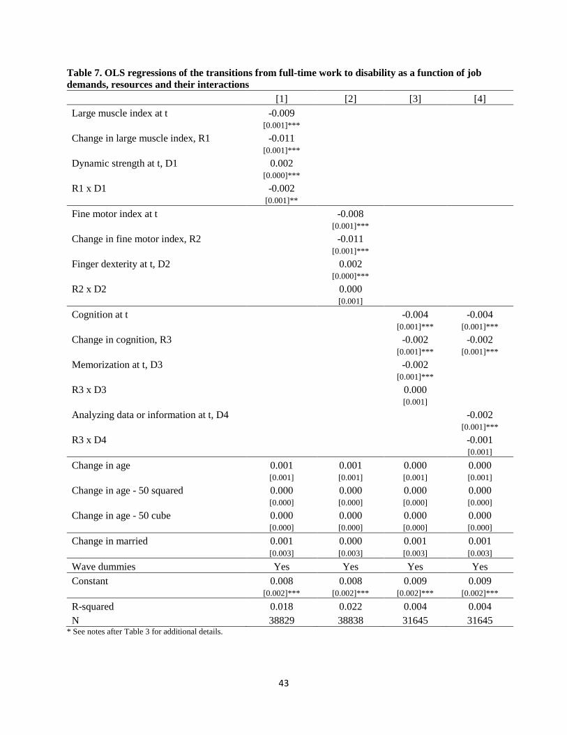
The interaction effects between the large-muscle index and dynamic strength job

demands are almost always strong and statistically significant, affecting work-limiting health

problems, depressive symptoms as measured by CESD, and work-to-disability transitions

(Tables 3 ,4 and 7). This means that developing large-muscle problems increases depressive

symptoms, reported work-limiting health problems, and work-to-disability transitions in all

occupations, but the effects are larger in occupations that demand dynamic strength. Only the

interaction in the regression of the transition from full-time work to retirement is not significant.

The interaction effects between fine-motor skills (resource) and finger dexterity (job

demand) as well as those between cognition and cognitive job demands are close to zero and

almost never statistically significant. The only exception is column 3 in Table 4, in which the

interaction term has an unexpectedly positive sign and is statistically significant at the 5% level.

The model predicts that cognitive decline increases depression relatively more in occupations

that do not demand memorization.

Overall, even though fine-motor skills and cognition strongly predict the five outcomes,

they do not seem to interact with job demands along these dimensions.

21

Appendix B reports results on additional outcome variables. We summarize the results

briefly here. The effects on the subjective probabilities of working past age 62 are similar to the

subjective probabilities of working past age 65. The two physical-decline measures are

statistically significant predictors of disliking work (i.e., of disagreeing or strongly disagreeing

with the statement that “I really enjoy going to work”), but cognitive decline is not. The

interactions of these measures with job demands are not statistically significant in the regression

on the dislike of work. The outcome variable is only available for workers—those not working at

t+1 are not in the analysis sample—and an important part of the sample is therefore missing and

may bias the coefficients toward zero. Decline in the large-muscle and the fine motor indices

make it less likely that an individual will switch employers, but none of the interaction effects

with job demands are statistically significant.

4.3. Robustness checks

Even though we use panel variation for identification, which we believe is more likely to

be valid than cross-section variation, our data are observational and therefore our estimates may

not capture the true causal effects of health on the outcome variables. This section discusses

alternative specifications and tests we performed to learn if there is evidence against our causal

interpretation.

First, Appendix A.5. provides simple descriptive tables showing mean changes in the

outcome variables by job demands and changes in resources. These tables use mean splits in the

explanatory variables and no controls. These specifications show the raw output without imposing

much structure on the data. The tables largely agree with the preferred regression results: changes

in any resources predict the outcome variables, but the effects are largest for large-muscle

resources in large muscle jobs.

22

Second, we estimated models with alternative sets of control variables. Our preferred

specification in Section 4.2. only used changes in a cubic function of age, changes in marital status

and wave indicators. Appendix tables C1-C5 show regressions of the five main outcome variables

using the following additional controls: gender, race, education, change in household income,

change in household wealth, change in spouse labor force status, whether employer sponsored DB

or DC retirement plans, whether self-employed, tenure at the main job, and whether health

insurance through employer or spouse. The main coefficients are indistinguishable from the

preferred ones reported in the previous section. We prefer using fewer controls, because some of

these additional controls are potential outcomes (such as whether the spouse works, or family

income), but it is reassuring that the control variables do not change our coefficients of interest,

perhaps because changes in health are relatively random in this age range.

Third, people in different jobs may have different trajectories in their health and/or the

outcome variables. For example, blue collar workers may face sharper declines in health and the

outcome variables compared to white collar workers. To explore this hypothesis, we estimated

placebo regressions on past values of three outcome variables as shown in Tables C6-C8. This test

was not feasible on the transition models. The main coefficients (changes in resources and

interactions with job demands) are close to zero and almost never statistically significant. One

exception is that apparently changes in fine motor skills are mildly correlated with past changes in

the subjective probabilities of working past age 65. Additionally, one more interaction coefficient

is significant at 5% and another one at 10%.

Fourth, retirement itself may simultaneously predict changes in health and the outcome

variables. To explore, we ran separate regressions on a narrower sample that included only full-

time workers at t and t+1. Appendix Table C9 shows the specification on three main outcomes

23

and the large muscle index. These models cannot be estimated on the transition models; and the

appendix only focuses on the large muscle index with the strongest results. Coefficients in these

regressions are likely biased toward zero because individuals who transition into retirement may

be worse off compared to those who remain in the labor force. Indeed, the coefficients are all closer

to zero compared to the preferred models. Nevertheless, changes in the large muscle index still

strongly predict all three outcomes, and the interaction terms are statistically significant at 5% in

two out of three cases and significant at 10% in the third case.

5. Discussion and conclusion

5.1. Summary

We used longitudinal data from the HRS to find how decline in individuals’ physical and

cognitive resources as well as the mismatch between resources and occupational job demands

affected various retirement-related outcomes. We considered three resource measures: 1) a large-

muscle index representing strength and overall physical fitness; 2) fine-motor skills representing

individuals’ ability to perform precise manipulations with their hands (as well as general

physical fitness); and 3) cognitive abilities that mostly focused on the quality of individuals’

working memories.

We paired these three resource measures with four corresponding job-demand measures

derived from the O*NET project. These were dynamic strength (paired with the large-muscle

index), finger dexterity (paired with fine-motor skills), memorization (paired with cognition) and

analyzing data and information (also paired with cognition).

We merged the O*NET characteristics with the detailed 3-digit occupations of HRS

participants and focused on five outcome variables: self-reported work-limiting health problems,

24

the number of depressive symptoms (as measured by the CESD scale), subjective probabilities of

working full-time after age 65, transitions from work to retirement, and to disability. We tested

whether HRS resources and O*NET job demands predicted these outcome variables. We

expected that the decline in resources would lead to more work-limiting problems, more

depressive symptoms, smaller subjective probabilities of working longer, and more transitions

out of work, especially in occupations that rely on specific skills. This latter effect was tested by

the interactions between resources and job demands.

The main novelty of our approach was to use panel econometric models when possible

that identified solely intra-personal rather than inter-personal variation in physical and cognitive

resources. Under reasonable assumptions this variation captures the causal effect of resource

decline on the outcomes. We were able to use panel econometric models because we had

repeated observations in our outcome variables that were collected among both working and

non-working individuals. In standard models of retirement transitions (which we also estimated)

such panel variation is not available to researchers, because (most) individuals retire only once.

Our approach therefore highlights a main advantage of using subjective probabilities such as the

chances of working full-time after age 65: they provide more variation both in the cross-section

(probabilities as opposed to 0-1 indicators available at the individual level) and over time (see

also Hurd 2009; Manski 2004).

We found that physical and cognitive resources all had a strong effect on the five

outcome variables. Decline in the physical measures (large-muscle and fine-motor) tended to

have a stronger effect than declines in cognitive abilities. For example, a decline of one standard

deviation in the large-muscle index decreased the subjective probability of working after age 65

25

by about 1.9 percentage points. The corresponding effect of cognitive ability was about half as

much at one percentage point.

The differences between physical and cognitive resources was even larger for CESD

depression. While a decline of one standard deviation in the large-muscle index increased the

number of depressive symptoms (out of 8) by about 0.21, a decline of one standard deviation in

cognition increased the number of such symptoms by 0.04 (both increases statistically significant

at 1%).

We also found that decline in the large-muscle index had a strong interaction effect with

dynamic strength job demands, implying the importance of mismatch in large muscle problems

for retirement. For example, an increase of one standard deviation from the mean in the

importance of dynamic strength on the job increased the effect of the large-muscle index on the

subjective probability of working past age 65 from 1.9 to 2.7 percentage points. Such an increase

also increased the effect on depressive symptoms from 0.21 to 0.25.

We found weak and statistically insignificant interaction effects between the fine-motor

index (resource) and finger dexterity (job demands), as well as between cognition (resource) and

memorization or analyzing data and information (job demands). There are several possible

explanations for this: It may be that fine motor skills and cognitive abilities are important

determinants of working in all occupations; or workers in cognitive and fine-motor occupations

may have good jobs that protect them from the adverse effects of mismatch (their employers may

accommodate the changing capabilities, or such workers may be able to switch to tasks or jobs

that better align with their reduced skills); or, finally, the pairing of the O*NET measures with

the HRS resource measures was not very good, which may have biased the interaction effect

toward zero.

26

5.2. Implications

Our findings demonstrate the importance for retirement research to consider the

considerable heterogeneity in individuals’ skills and in their jobs’ demands. Different jobs rely

on different skills. As workers age, their physical and cognitive resources decline, for some more

rapidly than for others. By simultaneously considering the heterogeneity in job demands and

resources, we showed that mismatch may be an important obstacle for the employability of some

workers, especially those working in occupations that rely on muscular endurance.

While we found that cognitive decline was associated with some outcomes (depressive

symptoms, retirement expectations, actual retirement), the association was considerably weaker

than with physical decline. We also did not find any interaction between cognitive decline and

job demands.

There are many potential reasons why decline in cognitive abilities is less crucial for

retirement outcomes. Workers in cognitively demanding jobs who experience declines in their

fluid cognitive abilities can rely on their crystallized intelligence (general knowledge and

experience) that is found to be more resistant to aging (Cattell 1987). Such workers also may be

in good jobs with more accommodating employers or have better outside options. Regardless,

cognitive decline appears to be less of a problem for workers at older ages than decline in

physical skills.

We found decline in fine-motor skills was a very strong predictor of retirement outcomes,

but we found little interaction effects with job demands.

We did find very large interaction effects between large-muscle problems and

corresponding job demands (dynamic strength). Employability in physically demanding jobs

27

appears to be very sensitive to an individual’s physical capabilities, or at least much more so than

employability in cognitive jobs is to declines in cognitive skills.

Workers in physically demanding jobs, thus, are more likely to face mismatch with the

demands of their jobs, especially those who experience a decline in their physical capabilities.

These mismatched workers are more likely to leave the labor force, perhaps because they are not

able to effectively work in their occupations and their options for work in other occupations are

limited. This is particularly a concern, because individuals in low socioeconomic status are both

overrepresented in physically demanding jobs, and are less financially prepared for retirement.

The fraction of the labor force in physical jobs has been shrinking in recent decades

(Brownson, Boehmer, and Luke, 2005; Sturm, 2004), and this trend may continue.

Consequently, age related mismatch may become a less important limitation for workers who

would like to continue working. But physical jobs still take up a non-trivial fraction of the

current labor force.

Delaying the decline in the physical health of these workers may increase the chances

that they can work to the ages they desired or had planned on. They may also be better off if their

employers accommodated their changing skills or if they could find alternative work

arrangements that better fit their abilities.

5.3. Limitations

There are several limitations to our study. We used observational data, and we could not

directly test the exogeneity of our explanatory variables. Our robustness checks and placebo

regressions, however, largely support our causal interpretation. Our models identify from

changes in resources (health), which are relatively random events.

28

The job-demand measures were defined by occupations, and so any heterogeneity within

occupations was ignored. We used occupational measures, because they are based on more

objective information than self-reported survey data and because O*NET provided a large

number of measures from which to choose. Future research might consider within-occupation

heterogeneity in job demands.

The two physical-resource measures may be too general and focused on problems for

individuals at older ages than those analyzed. This is particularly true for the fine-motor index

that included problems with eating and dressing. Such issues are rare in the working-age

population and typically manifest long after an individual leaves the labor force. This may

explain why we found no interaction effects between the fine-motor index and the corresponding

job demand (finger dexterity).

An important element of our methods was pairing HRS resource measures with O*NET

job characteristics and to analyze the interactions between these. The success of this method

depends on the quality of the pairing. If the resource and the job-demand measures are

misaligned because, for example, they correspond to somewhat different factors, then we would

expect muted coefficients. This problem may have contributed to the lack of significance

between the fine-motor index and finger dexterity, but we think the quality of the other pairs was

better.

Our preferred sample included those non-workers who had a job in the previous HRS

waves. But before 2006 the HRS did not ask the subjective probability of working after ages

62/65 question of some non-workers. We imputed these cases using a relatively simple single-

imputation methodology that flexibly included age, gender, labor force status and past

expectations. Imputation, however, is never perfect. In the future, when more HRS waves

29

become available, researchers might estimate similar models using only post-2006 data that need

no imputation.

30

References

Data

Health and Retirement Study, waves 1992-2012, public use dataset. Produced and distributed by

the University of Michigan with funding from the National Institute on Aging (grant

number NIA U01AG009740). Ann Arbor, MI.

RAND HRS Data, Version P. Produced by the RAND Center for the Study of Aging, with

funding from the National Institute on Aging and the Social Security Administration.

Santa Monica, CA (August 2016).

Research Studies

Acemoglu, Daron, and David Autor. 2011. "Skills, tasks and technologies: Implications for

employment and earnings." In Handbook of labor economics, 1043-1171. Elsevier.

Angrisani, Marco, Arie Kapteyn, and Erik Meijer. 2015. "Nonmonetary job characteristics and

employment transitions at older ages."

Atalay, K, and Garry F. Barrett. 2014. "The causal effect of retirement on health: New evidence

from Australian pension reform." Economics Letters, 125 (3): 392-395.

Autor, David H, Frank Levy, and Richard J Murnane. 2003. "The skill content of recent

technological change: An empirical exploration." The Quarterly Journal of Economics

118 (4):1279-1333.

Belbase, Anek, Geoffrey T Sanzenbacher, and Christopher M Gillis. 2016. "How do job skills

that decline with age affect white-collar workers?" Issue brief:16-6.

Ben-Porath, Yoram. 1967. "The production of human capital and the life cycle of earnings."

Journal of Political Economy 75 (4, Part 1):352-365.

31

Blundell, Richard, Jack Britton, Monica Costa Dias, and Eric French. 2017. "The impact of

health on labour supply near retirement." IFS Working Papers W17/18, Institute for

Fiscal Studies.

Bowlus, Audra, Hiroaki Mori, and Chris Robinson. 2016. "Ageing and Skill Portfolios: Evidence

from Job Based Skill Measures. " The Journal of the Economics of Ageing, 7: 89-103.

Brownson, Ross C, Tegan K Boehmer, and Douglas A Luke. 2005. "Declining Rates of Physical

Activity in the United States: What are the Contributors? " Annual review of public

health. 26 (1):421-43.

Cahill, Kevin E, Michael D Giandrea, and Joseph F Quinn. 2006. "Retirement patterns from

career employment." The Gerontologist 46 (4):514-523.

Cappelli, Peter H. 2015. "Skill gaps, skill shortages, and skill mismatches: Evidence and

arguments for the United States." ILR Review 68 (2):251-290.

Carmeli, Eli, Hagar Patish, and Raymond Coleman. 2003. "The aging hand." The Journals of

Gerontology Series A: Biological Sciences and Medical Sciences 58 (2):M146-M152.

Carr, D. C., Castora-Binkley, M., Kail, B. K., Willis, R. J., & Carstensen L. 2016. Does Job

Complexity Offer Protection Against the Mental Retirement Effect? Working paper.

Cattell, Raymond Bernard. 1987. Intelligence: Its Structure, Growth and Action. Vol. 35:

Elsevier.

Crimmins, Eileen M, Jung Ki Kim, Kenneth M Langa, and David R Weir. 2011. "Assessment of

cognition using surveys and neuropsychological assessment: the Health and Retirement

Study and the Aging, Demographics, and Memory Study." Journals of Gerontology

Series B: Psychological Sciences and Social Sciences 66 (suppl_1):i162-i171.

32

Del Missier, Fabio, Timo Mäntylä, Patrik Hansson, Wändi Bruine de Bruin, Andrew M Parker,

and Lars-Göran Nilsson. 2013. "The multifold relationship between memory and decision

making: An individual-differences study." Journal of Experimental Psychology:

Learning, Memory, and Cognition 39 (5):1344.

Dillon, Eleanor Wiske, and Jeffrey Andrew Smith. 2017. "Determinants of the match between

student ability and college quality." Journal of Labor Economics 35 (1):45-66.

Fisher, Gwenith G, Dorey S Chaffee, and Amanda Sonnega. 2016. "Retirement timing: A review

and recommendations for future research." Work, Aging and Retirement 2 (2):230-261.

Fisher, GG, Halimah Hassan, Jessica D Faul, Willard L Rodgers, and David R Weir. 2015.

"Health and retirement study imputation of cognitive functioning measures: 1992–2010."

Ann Arbor: University of Michigan.

Hoogendam, Yoo Young, Fedde van der Lijn, Meike W Vernooij, Albert Hofman, Wiro J

Niessen, Aad van der Lugt, M Arfan Ikram, and Jos N van der Geest. 2014. "Older age

relates to worsening of fine motor skills: a population-based study of middle-aged and

elderly persons." Frontiers in Aging Neuroscience 6:259.

Hudomiet, Péter. 2015. The role of occupation specific adaptation costs in explaining the

educational gap in unemployment. Working paper.

Hurd, Michael. 2009. "Subjective Probabilities in Household Surveys." Annual Review of

Economics 1:543-562. doi: Doi 10.1146/annurev.economics.050708.142955.

Insler, Michael. 2014. "The Health Consequences of Retirement," Journal of Human Resources

49 (1):195-233.

James, Jonathan. 2011. "Ability matching and occupational choice." Working paper 1125,

Federal Reserve Bank of Cleveland.

33

Liebermann, Susanne C, Jürgen Wegge, and Andreas Müller. 2013. "Drivers of the expectation

of remaining in the same job until retirement age: A working life span demands-resources

model." European Journal of Work and Organizational Psychology 22 (3):347-361.

Lindenlaub, Ilse. 2017. "Sorting Multidimensional Types: Theory and Application." Review of

Economic Studies, 84 (2):718-789.

Manski, Charles. 2004. "Measuring Expectations." Econometrica 72 (5):1329-1376.

Mazzonna, Fabrizio, and Franco Peracchi. 2017. "Unhealthy Retirement?" Journal of Human

Resources, University of Wisconsin Press 52 (1): 128-151.

McGarry, Kathleen. 2004. "Health and retirement: do changes in health affect retirement

expectations?" Journal of Human Resources 39 (3):624-648.

McGonagle, Alyssa K, Gwenith G Fisher, Janet L Barnes-Farrell, and James W Grosch. 2015.

"Individual and work factors related to perceived work ability and labor force outcomes."

Journal of Applied Psychology 100 (2):376.

Rice, Neil E, Iain A Lang, William Henley, and David Melzer. 2010. "Common health predictors

of early retirement: findings from the English Longitudinal Study of Ageing." Age and

Ageing 40 (1):54-61.

van Rijn, Rogier M, Suzan JW Robroek, Sandra Brouwer, and Alex Burdorf. 2014. "Influence of

poor health on exit from paid employment: a systematic review." Occupational and

Environmental Medicine 71 (4):295-301.

Pei, Zhuan, Pischke, Jörn-Steffen, and Schwandt, Hannes. 2017. "Poorly Measured Confounders

are More Useful on the Left Than on the Right," NBER Working Papers 23232, National

Bureau of Economic Research, Inc.

34

Rohwedder, S., & Willis, R. J. 2010. "Mental retirement." Journal of Economic Perspectives, 24,

119-38.

Roy, Andrew Donald. 1951. "Some thoughts on the distribution of earnings." Oxford Economic

Papers 3 (2):135-146.

Schwandt, Hannes. 2018. "Wealth Shocks and Health Outcomes: Evidence from Stock Market

Fluctuations." American Economic Journal: Applied Economics, 10 (4):349–377.

Sonnega, Amanda, Brooke Helppie-McFall, Peter Hudomiet, Robert J Willis, and Gwenith G

Fisher. 2017. "A comparison of subjective and objective job demands and fit with

personal resources as predictors of retirement timing in a national US sample." Work,

Aging and Retirement 4 (1):37-51.

Sturm, Roland. 2004. "The economics of physical activity: Societal trends and rationales for

interventions. " American Journal of Preventive Medicine, 27 (3):126-135.

Topa, Gabriela, Juan Antonio Moriano, Marco Depolo, Carlos-María Alcover, and J Francisco

Morales. 2009. "Antecedents and consequences of retirement planning and decision-

making: A meta-analysis and model." Journal of Vocational Behavior 75 (1):38-55.

Wang, Mo, and Kenneth S Shultz. 2010. "Employee retirement: A review and recommendations

for future investigation." Journal of Management 36 (1):172-206.

Willis, Robert J, and Sherwin Rosen. 1979. "Education and self-selection." Journal of political

Economy 87 (5, Part 2):S7-S36.

Willis, Robert J. 1986. "Wage determinants: A survey and reinterpretation of human capital

earnings functions." Handbook of labor economics 1:525-602.

Yamaguchi, Shintaro. 2012. "Tasks and heterogeneous human capital." Journal of Labor

Economics 30 (1):1-53.

35

Yamaguchi, Shintaro. 2016. "Changes in returns to task-specific skills and gender wage gap."

Journal of Human Resources:1214-6813R2.

36

Tables and Figures

Figure 1. Age patterns in whether health limits working and three resource measures, non-parametric regressions, HRS, Age 50-70, 1994-2014, unweighted

Panel A: Whether health limits work Panel B: Large muscle index

Panel C: Fine motor skills index Panel D: Cognition

*The three resource measures are standardized to have zero mean and standard deviation of one among 50-70 years old full-time workers, but the graphs include everyone regardless of labor force status. Higher values indicate better health. The confidence intervals assume i.i.d. data, and they are likely too narrow due to the positive correlations in the panel.

37

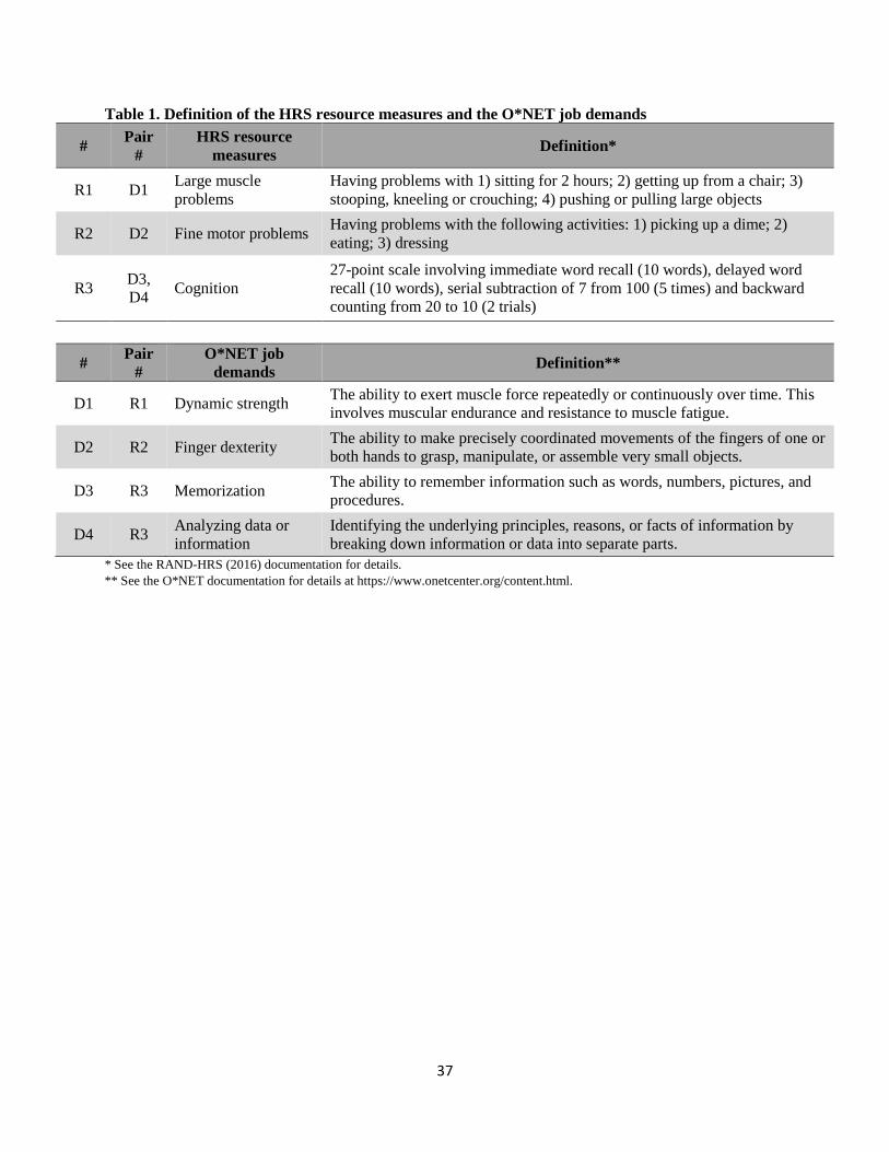
Table 1. Definition of the HRS resource measures and the O*NET job demands

# Pair #

HRS resource measures Definition*

R1 D1 Large muscle problems

Having problems with 1) sitting for 2 hours; 2) getting up from a chair; 3) stooping, kneeling or crouching; 4) pushing or pulling large objects

R2 D2 Fine motor problems Having problems with the following activities: 1) picking up a dime; 2) eating; 3) dressing

R3 D3, D4 Cognition

27-point scale involving immediate word recall (10 words), delayed word recall (10 words), serial subtraction of 7 from 100 (5 times) and backward counting from 20 to 10 (2 trials)

# Pair #

O*NET job demands Definition**

D1 R1 Dynamic strength The ability to exert muscle force repeatedly or continuously over time. This involves muscular endurance and resistance to muscle fatigue.

D2 R2 Finger dexterity The ability to make precisely coordinated movements of the fingers of one or both hands to grasp, manipulate, or assemble very small objects.

D3 R3 Memorization The ability to remember information such as words, numbers, pictures, and procedures.

D4 R3 Analyzing data or information

Identifying the underlying principles, reasons, or facts of information by breaking down information or data into separate parts.

* See the RAND-HRS (2016) documentation for details. ** See the O*NET documentation for details at https://www.onetcenter.org/content.html.

38

Table 2. Descriptive statistics of the main variables, HRS, Age 50-70, full-time workers, unweighted N mean sd min max Age 46935 57.9 4.597 50 70 Female 46935 0.477 0.499 0 1 White 46935 0.767 0.423 0 1 Black 46935 0.163 0.369 0 1 Other race 46935 0.070 0.256 0 1 Hispanic 46935 0.106 0.308 0 1 High school dropout 46935 0.177 0.382 0 1 High school graduate 46935 0.285 0.452 0 1 College dropout 46935 0.258 0.438 0 1 College graduate 46935 0.280 0.449 0 1 Married 46935 0.713 0.452 0 1 Spouse works 46935 0.493 0.500 0 1 Household income 46935 90797 147927 0 13570429 Total household wealth 46935 355945 1086466 -4383000 90648200 Has a DB pension 46935 0.326 0.469 0 1 Has a DC pension 46935 0.397 0.489 0 1 Self employed 46935 0.158 0.365 0 1 Tenure at job, in years 46935 13.747 11.494 0 55 Has health insurance from employer 46935 0.680 0.467 0 1 Has health insurance from spouse 46935 0.149 0.356 0 1 HRS interview wave 46935 6.933 3.236 2 12 Dynamic strength, O*NET 46935 0.178 0.126 0.000 0.562 Finger dexterity, O*NET 46935 0.393 0.097 0.177 0.718 Memorization, O*NET 46935 0.339 0.080 0.104 0.580 Analyzing data or information, O*NET 46935 0.523 0.147 0.157 0.877 Large muscle problem index 46927 0.740 1.075 0 4 Fine motor problem index 46935 0.047 0.236 0 3 Cognition 39357 17.020 3.876 0 27 Full-time work → retirement transition 39699 0.104 0.306 0 1 Full-time work → disability transition 39699 0.008 0.087 0 1 Subjective probability working full time after age 62 34674 57.053 36.894 0 100 Subjective probability working full time after age 65 37449 36.661 35.693 0 100 Health limits work 46651 0.078 0.267 0 1 CESD depression score 43876 1.088 1.665 0 8 Moves to a different employer 33158 0.094 0.292 0 1 Does not enjoy going to work 42991 0.121 0.326 0 1

39

Table 3. OLS regressions of the change in whether health limits working as a function of job demands, resources and their interactions [1] [2] [3] [4] Large muscle index at t -0.038

[0.002]*** Change in large muscle index, R1 -0.075

[0.003]*** Dynamic strength at t, D1 0.007

[0.001]*** R1 x D1 -0.012

[0.003]*** Fine motor index at t -0.026

[0.003]*** Change in fine motor index, R2 -0.044

[0.002]*** Finger dexterity at t, D2 0.005

[0.001]*** R2 x D2 0.000 [0.002]

Cognition at t -0.011 -0.010 [0.002]*** [0.002]***

Change in cognition, R3 -0.010 -0.010 [0.002]*** [0.002]***

Memorization at t, D3 -0.008 [0.002]***

R3 x D3 -0.003 [0.002]

Analyzing data or information at t, D4 -0.008 [0.002]***

R3 x D4 0.001 [0.002]

Change in age -0.019 -0.018 -0.021 -0.021 [0.005]*** [0.005]*** [0.005]*** [0.005]***

Change in age - 50 squared 0.001 0.001 0.001 0.001 [0.000]** [0.000]** [0.000]*** [0.000]***

Change in age - 50 cube 0.000 0.000 0.000 0.000 [0.000] [0.000] [0.000] [0.000]

Change in married 0.006 0.002 0.006 0.006 [0.010] [0.010] [0.011] [0.011]

Wave dummies Yes Yes Yes Yes Constant 0.052 0.048 0.049 0.048 [0.008]*** [0.009]*** [0.009]*** [0.009]***

R-squared 0.045 0.026 0.006 0.006 N 38272 38279 31149 31149

*Sample: HRS, Age 50-70, full-time workers at t, valid interviews at t+1, and non-missing resources and outcome. Job demands and resources are standardized and higher values indicate higher demands and more resources (better health). Change measures are all defined from wave t to t+1. Robust standard errors clustered on the household id are in brackets. *, **, and *** indicate statistical significance at 10, 5, and 1% respectively.

40

Table 4. OLS regressions of the change in the CESD depressive symptoms as a function of job demands, resources and their interactions [1] [2] [3] [4] Large muscle index at t -0.043



[0.007]** R1 x D1 -0.040




[0.007]* R2 x D2 0.004 [0.012]

Cognition at t -0.004 -0.002 [0.010] [0.010]


Memorization at t, D3 -0.013 [0.008]

R3 x D3 0.023 [0.012]**

Analyzing data or information at t, D4 -0.019 [0.008]**

R3 x D4 0.015 [0.012]

Change in age 0.030 0.036 0.021 0.021 [0.027] [0.027] [0.028] [0.028]

Change in age - 50 squared -0.001 -0.001 -0.001 -0.001 [0.002] [0.002] [0.002] [0.002]


Change in married -0.482 -0.489 -0.484 -0.484 [0.065]*** [0.065]*** [0.068]*** [0.068]***

Wave dummies Yes Yes Yes Yes Constant 0.024 0.016 0.051 0.051 [0.047] [0.047] [0.048] [0.048]

R-squared 0.020 0.013 0.009 0.009 N 35720 35724 31623 31623

*See notes after Table 3 for additional details.

41

Table 5. OLS regressions of the change in the subjective probabilities of working full-time after age 65 as a function of job demands, resources and their interactions [1] [2] [3] [4] Large muscle index at t 1.252

[0.166]*** Change in large muscle index, R1 1.921

[0.243]*** Dynamic strength at t, D1 -0.297

[0.152]* R1 x D1 0.820

[0.237]*** Fine motor index at t 1.105

[0.208]*** Change in fine motor index, R2 1.010

[0.196]*** Finger dexterity at t, D2 -0.041

[0.149] R2 x D2 0.120 [0.182]

Cognition at t 0.676 0.644 [0.221]*** [0.219]***

Change in cognition, R3 1.049 1.027 [0.271]*** [0.269]***

Memorization at t, D3 0.498 [0.177]***

R3 x D3 -0.221 [0.254]

Analyzing data or information at t, D4 0.580 [0.172]***

R3 x D4 -0.246 [0.245]

Change in age 1.009 0.944 0.785 0.787 [0.594]* [0.595] [0.622] [0.622]



Change in married -1.863 -1.762 -1.686 -1.692 [1.166] [1.170] [1.251] [1.252]

Wave dummies Yes Yes Yes Yes Constant -2.230 -2.144 -1.997 -1.999 [0.994]** [0.995]** [1.016]** [1.016]**

R-squared 0.008 0.006 0.006 0.006 N 28176 28177 24798 24798

* Subjective probabilities of working are only collected in non-proxy interviews from people younger than age 65. Prior to 2006, the HRS did not ask this question from non-workers. The values of expectations for the 50-64-year-old non-proxy non-workers are imputed with a model described in Appendix A. See notes after Table 3 for additional details.

42

Table 6. OLS regressions of the transitions from full-time work to retirement as a function of job demands, resources and their interactions [1] [2] [3] [4] Large muscle index at t -0.028



[0.001]*** R1 x D1 -0.002

[0.002] Fine motor index at t -0.020



[0.002]*** R2 x D2 0.000 [0.002]

Cognition at t -0.015 -0.015 [0.002]*** [0.002]***


Memorization at t, D3 -0.004 [0.002]**

R3 x D3 -0.001 [0.002]


R3 x D4 -0.001 [0.002]

Change in age -0.056 -0.057 -0.054 -0.054 [0.004]*** [0.004]*** [0.004]*** [0.004]***

Change in age - 50 squared 0.004 0.004 0.004 0.004 [0.000]*** [0.000]*** [0.000]*** [0.000]***


Change in married -0.001 -0.003 0.001 0.001 [0.009] [0.009] [0.010] [0.010]


R-squared 0.061 0.057 0.051 0.051 N 38829 38838 31645 31645

* See notes after Table 3 for additional details.

43

Table 7. OLS regressions of the transitions from full-time work to disability as a function of job demands, resources and their interactions [1] [2] [3] [4] Large muscle index at t -0.009



[0.000]*** R1 x D1 -0.002

[0.001]** Fine motor index at t -0.008



[0.000]*** R2 x D2 0.000 [0.001]

Cognition at t -0.004 -0.004 [0.001]*** [0.001]***



R3 x D3 0.000 [0.001]


R3 x D4 -0.001 [0.001]

Change in age 0.001 0.001 0.000 0.000 [0.001] [0.001] [0.001] [0.001]

Change in age - 50 squared 0.000 0.000 0.000 0.000 [0.000] [0.000] [0.000] [0.000]




R-squared 0.018 0.022 0.004 0.004 N 38829 38838 31645 31645

* See notes after Table 3 for additional details.

44

Appendix A: Additional information about the data and the sample

A.1. Measurement of job demands

The O*NET database contains measures for 974 occupations, corresponding to the

occupations in the most recent HRS. However, the occupational coding schemes in the restricted

HRS data have changed over time (Nolte, Turf, and Servais 2014). To ensure comparability across

waves of HRS data, we use a coding scheme that is consistent over time and that aggregates across

small, similar occupation groups. This coding scheme was developed to use in conjunction with

the O*NET data and contains 192 separate occupations/occupational groupings derived from the

original occupational codes.10

If HRS respondents report working more than one job HRS elicits and codes the occupation

information for all jobs a respondent may hold. The interview also asks respondents to name the

job they consider to be their main occupation, which is the occupation we use here.

For each occupation in the database, O*NET provides information on the level and

importance of each required work activity. Following Firpo, Fortin, and Lemieux (2011), we use

Cobb-Douglas weighted means to combine occupation-level importance and level measures.

Importance weights are 2/3; level weights are 1/3. Given the smaller number of somewhat

aggregated occupations in our HRS data, we average across multiple O*NET occupations that

crosswalk to the HRS occupation categories to create O*NET measures for the HRS occupations.

10 The coding scheme was originally developed by Peter Hudomiet for his dissertation, and it has been used by a number of researchers since then (e.g. Carr et al., 2016; Sonnega et al. 2018). It can be accessed at https://sites.google.com/site/phudomiet/Occupation-Crosswalks-MRRC-2015.xlsx.

45

We use CPS detailed occupation frequencies to weight O*NET measures to the level of the 192

detailed occupation categories used in this paper.

The HRS typically only asks about workers’ occupations if they reported a change in their

employment situation (different employer or different tasks at the same employer) or they are

newly recruited sample members. To maximize the available information, workers with missing

occupations were imputed their previously reported occupations. Of the 46,935 person-year

observations in our total sample 20,457 (43.6%) occupations were carried forward from earlier

waves. 20,254 of them (43.2%) reported to have the same employer and job title as in the previous

wave; and 203 of them (0.4%) were missing for other reasons. Our results are virtually identical if

the latter 203 cases are excluded from the sample.

A.2. Imputations

Beginning in 2006, the HRS asked all respondents their subjective probabilities of working

full-time after age 62 and 65. Prior to 2006, however, non-working individuals were only asked

about the probabilities that they would ever work, resulting in partial responses to P65: a 0%

answer implies a 0% chance of working full-time after ages 62 or 65. Those, who provided a non-

zero answer before 2006, however, were not followed up with a question about full-time work

after ages 62 and 65.

We seek to include in our sample those who currently do not work but who did work in the

prior wave. Because expectations of such individuals are partially missing before 2006, we

developed a regression-based imputation model estimated over complete data from 2006 to 2014,

reported in Table A1.

46

Table A1. Imputation model used to impute the subjective probabilities of working full-time after age 62 and 65, HRS, Age 50-61 (column 1) and Age 50-64 (column 2), non-proxy, non-workers in the current wave, full-time workers in the previous wave, reported a positive chance of working in the future, 2006-2014 pw62 pw65

Age - 50 (A) -0.15 -0.952 [0.639] [0.336]***

Age - 50 squared (A2) -0.004 0.046 [0.035] [0.015]***

Age - 50 cube (A3) 2.538 5.644 [3.533] [2.353]**

Female (F) 1.419 2.197 [2.961] [2.096] Retired ref. ref. Unemployed (U) 43.224 29.404

[6.455]*** [5.032]*** Disabled (D) 31.404 16.137

[11.037]*** [8.899]* OLF other reason (O) 21.322 20.842

[9.459]** [8.277]** U x A -1.725 -0.926

[0.761]** [0.505]* D x A -1.613 -0.428

[1.403] [1.042] O x A 0.38 -0.127 [1.071] [0.844] U x F -3.087 -2.757

[4.085] [3.222] D x F -7.553 -10.837

[7.336] [6.482]* O x F -0.31 -10.054

[7.302] [6.176] Lagged Pr(works after 62) 0.27

[0.027]*** Lagged Pr(works after 65) 0.298 [0.023]*** Constant 1.349 -3.941

[7.623] [6.183] R-squared 0.323 0.256 N 977 1328

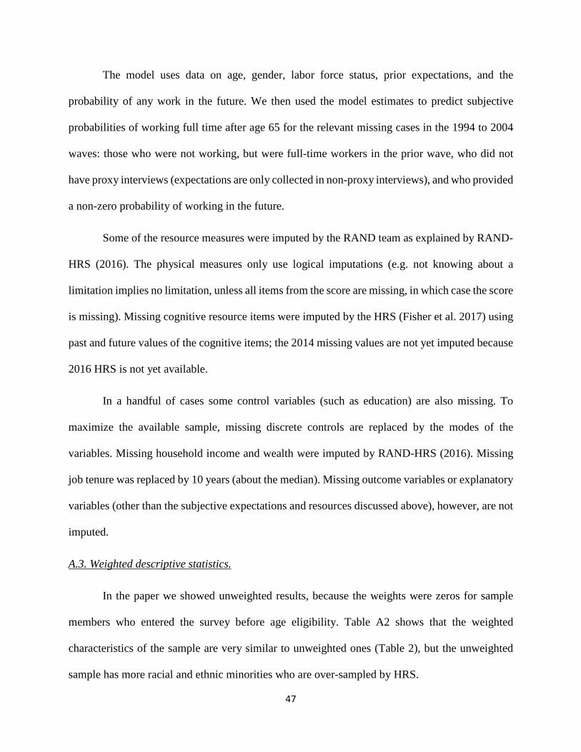
47

The model uses data on age, gender, labor force status, prior expectations, and the

probability of any work in the future. We then used the model estimates to predict subjective

probabilities of working full time after age 65 for the relevant missing cases in the 1994 to 2004

waves: those who were not working, but were full-time workers in the prior wave, who did not

have proxy interviews (expectations are only collected in non-proxy interviews), and who provided

a non-zero probability of working in the future.

Some of the resource measures were imputed by the RAND team as explained by RAND-

HRS (2016). The physical measures only use logical imputations (e.g. not knowing about a

limitation implies no limitation, unless all items from the score are missing, in which case the score

is missing). Missing cognitive resource items were imputed by the HRS (Fisher et al. 2017) using

past and future values of the cognitive items; the 2014 missing values are not yet imputed because

2016 HRS is not yet available.

In a handful of cases some control variables (such as education) are also missing. To

maximize the available sample, missing discrete controls are replaced by the modes of the

variables. Missing household income and wealth were imputed by RAND-HRS (2016). Missing

job tenure was replaced by 10 years (about the median). Missing outcome variables or explanatory

variables (other than the subjective expectations and resources discussed above), however, are not

imputed.

A.3. Weighted descriptive statistics.

In the paper we showed unweighted results, because the weights were zeros for sample

members who entered the survey before age eligibility. Table A2 shows that the weighted

characteristics of the sample are very similar to unweighted ones (Table 2), but the unweighted

sample has more racial and ethnic minorities who are over-sampled by HRS.

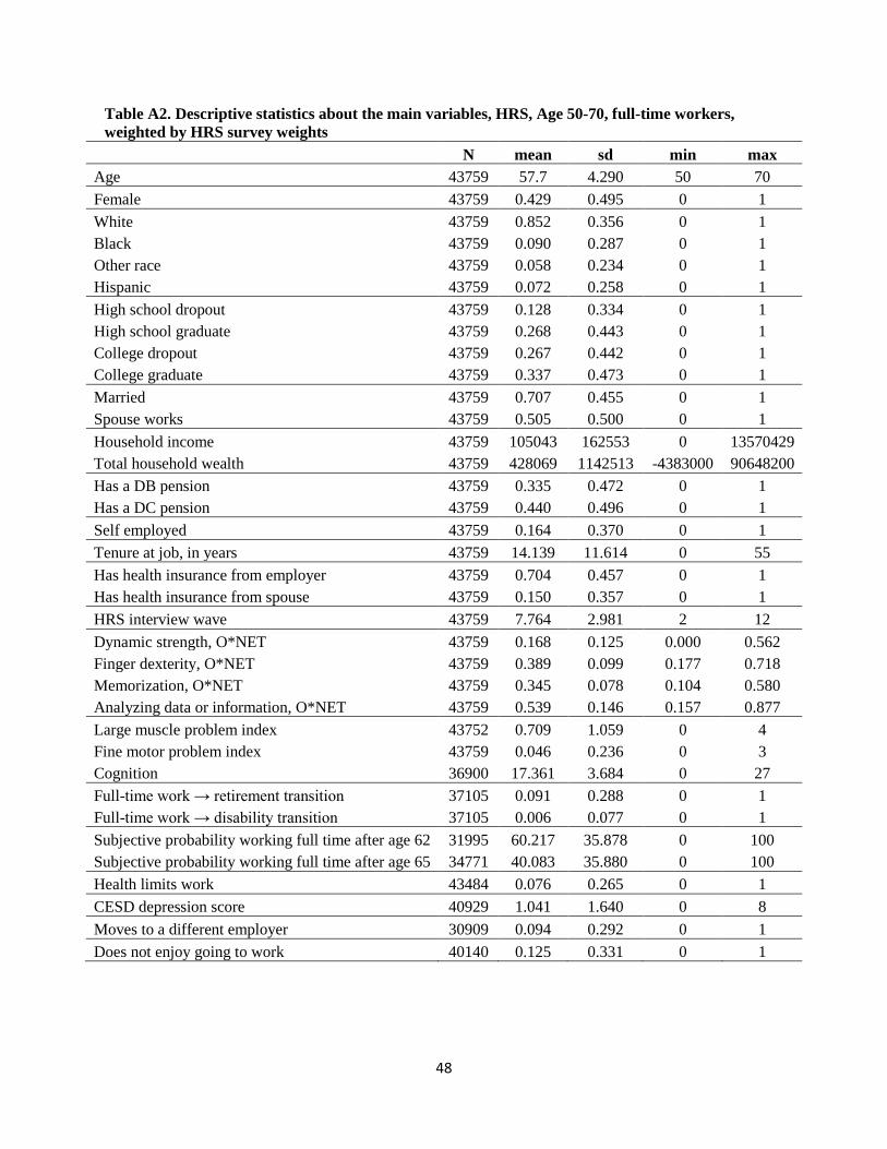
48

Table A2. Descriptive statistics about the main variables, HRS, Age 50-70, full-time workers, weighted by HRS survey weights

N mean sd min max Age 43759 57.7 4.290 50 70 Female 43759 0.429 0.495 0 1 White 43759 0.852 0.356 0 1 Black 43759 0.090 0.287 0 1 Other race 43759 0.058 0.234 0 1 Hispanic 43759 0.072 0.258 0 1 High school dropout 43759 0.128 0.334 0 1 High school graduate 43759 0.268 0.443 0 1 College dropout 43759 0.267 0.442 0 1 College graduate 43759 0.337 0.473 0 1 Married 43759 0.707 0.455 0 1 Spouse works 43759 0.505 0.500 0 1 Household income 43759 105043 162553 0 13570429 Total household wealth 43759 428069 1142513 -4383000 90648200 Has a DB pension 43759 0.335 0.472 0 1 Has a DC pension 43759 0.440 0.496 0 1 Self employed 43759 0.164 0.370 0 1 Tenure at job, in years 43759 14.139 11.614 0 55 Has health insurance from employer 43759 0.704 0.457 0 1 Has health insurance from spouse 43759 0.150 0.357 0 1 HRS interview wave 43759 7.764 2.981 2 12 Dynamic strength, O*NET 43759 0.168 0.125 0.000 0.562 Finger dexterity, O*NET 43759 0.389 0.099 0.177 0.718 Memorization, O*NET 43759 0.345 0.078 0.104 0.580 Analyzing data or information, O*NET 43759 0.539 0.146 0.157 0.877 Large muscle problem index 43752 0.709 1.059 0 4 Fine motor problem index 43759 0.046 0.236 0 3 Cognition 36900 17.361 3.684 0 27 Full-time work → retirement transition 37105 0.091 0.288 0 1 Full-time work → disability transition 37105 0.006 0.077 0 1 Subjective probability working full time after age 62 31995 60.217 35.878 0 100 Subjective probability working full time after age 65 34771 40.083 35.880 0 100 Health limits work 43484 0.076 0.265 0 1 CESD depression score 40929 1.041 1.640 0 8 Moves to a different employer 30909 0.094 0.292 0 1 Does not enjoy going to work 40140 0.125 0.331 0 1

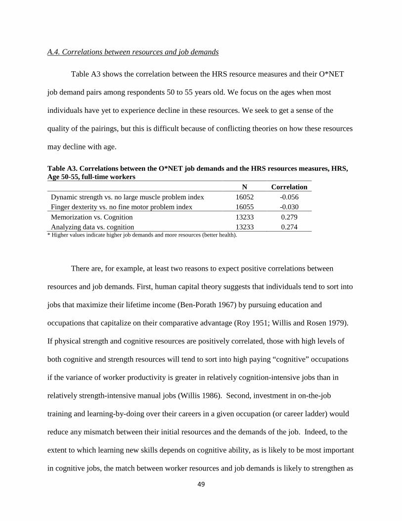
49

A.4. Correlations between resources and job demands

Table A3 shows the correlation between the HRS resource measures and their O*NET

job demand pairs among respondents 50 to 55 years old. We focus on the ages when most

individuals have yet to experience decline in these resources. We seek to get a sense of the

quality of the pairings, but this is difficult because of conflicting theories on how these resources

may decline with age.

Table A3. Correlations between the O*NET job demands and the HRS resources measures, HRS, Age 50-55, full-time workers N Correlation Dynamic strength vs. no large muscle problem index 16052 -0.056 Finger dexterity vs. no fine motor problem index 16055 -0.030 Memorization vs. Cognition 13233 0.279 Analyzing data vs. cognition 13233 0.274

* Higher values indicate higher job demands and more resources (better health).

There are, for example, at least two reasons to expect positive correlations between

resources and job demands. First, human capital theory suggests that individuals tend to sort into

jobs that maximize their lifetime income (Ben-Porath 1967) by pursuing education and

occupations that capitalize on their comparative advantage (Roy 1951; Willis and Rosen 1979).

If physical strength and cognitive resources are positively correlated, those with high levels of

both cognitive and strength resources will tend to sort into high paying “cognitive” occupations

if the variance of worker productivity is greater in relatively cognition-intensive jobs than in

relatively strength-intensive manual jobs (Willis 1986). Second, investment in on-the-job

training and learning-by-doing over their careers in a given occupation (or career ladder) would

reduce any mismatch between their initial resources and the demands of the job. Indeed, to the

extent to which learning new skills depends on cognitive ability, as is likely to be most important

in cognitive jobs, the match between worker resources and job demands is likely to strengthen as

50

job tenure increases. In addition, investments in health capital (Grossman 1972) to maintain

physical and mental health during the career would be important in maintaining match-quality.

At the same time, there is at least one reason to expect negative correlations between

resources and job demands. Specifically, too much exposure to the demands of a job may deplete

individuals’ resources, leading to a negative correlation between their resources and job

demands. For example, exposure to repeated heavy physical activities may lead to physical

health issues. We do not expect this mechanism to play a role in cognition.

Table A3 shows that there are large positive correlations between cognitive ability and

the two cognitive job demands, each with a correlation coefficient of about 0.3. This suggests

that individuals with high cognitive abilities sort into cognitively demanding jobs, or that

individuals occupying cognitively demanding jobs experience slower declines in cognition

whether or not the job is causal for the reduced decline. These mechanisms may operate

simultaneously.

At the same time, we found small negative correlations between the physical resources

and job demands. This may mean that sorting into physical jobs and learning-by-doing are less

important for physical attributes and that, instead, depletion of physical resources does occur in

physically demanding jobs (Fraade-Blanar et al. 2017). It is also possible that workers in

physically demanding jobs have riskier habits (e.g., smoking, heavy drinking) than workers in

less physically demanding jobs, leading to depletion of their resources relevant to such jobs.

Finally, the physical resource and job-demand measures may not pair well, because they

correspond to different attributes of individuals. In such a case, we would not expect a strong

interaction effect between these measures in the retirement regressions.

51

A.5. Descriptive patterns in resources, job demands and the various outcome variables

Tables A4 through A7 show how the change in resources when interacted with job

demands predict the main outcome variables: work-limiting health problems, depressive

symptoms, and expectations to work in the future. Here we seek descriptive evidence from data

without imposing modeling assumptions. The main patterns we are looking for are increased

mismatches between job demands and personal resources as physical and cognitive resources

decline, and for differences in mismatches for workers in jobs with high versus low demand for a

given resource.

Each table focuses on a separate dimension of job demands and workers’ corresponding

resources. Table A4 shows the results for the large muscle index. The cells of the table show the

means of the outcome variables at wave t and t+1. The rows of the table indicate transitions in

the workers’ resource measures as observed across two waves in the HRS data: from high (above

the mean) or low (below the mean) at wave t to high/low at t+1. The columns indicate the waves

(t and t+1) with the left panel showing results for workers in occupations with high demand for

dynamic strength (O*NET index above the mean) and the right panel showing results for

workers in occupations with low demand for dynamic strength (O*NET index below the mean).

We expect larger changes in the outcome variables from wave t to t+1 when individuals’

resources (HRS large muscle index) decline from high to low, especially in jobs that demand

those resources.

Health limitations increase over two-year periods as shown by the line “all” in the first

panel: among those with jobs that have a high demand for dynamic strength, 8.3% had a

limitation in the initial wave and 13.5% had a limitation in the following wave; among those

with jobs that have a low demand, 6.1% had a limitation in the initial wave and 9.2% had a

52

limitation in the following wave It is notable that both the initial level and the rate of increase

are greater when the job has high demand for dynamic strength than when the job has low

demand.

Among individuals who score high on the large muscle index at both waves t and t+1

(workers’ resources observed in HRS: high high), very few report any work-limiting health

problems. Specifically, only 2.2% of such individuals in occupations demanding a lot of dynamic

strength report work-limiting health problems at t, and only 3.3% report such problems at t+1.

Among workers who score high on the large muscle index in both t and t+1 and who are in

occupations with relatively low demand for dynamic strength, less than 3 percent report any

work-limiting health problems at either t or t+1.

Among individuals for whom the large-muscle index deteriorates from high to low, there

is a sharp increase in reported work-limiting health problems, especially in occupations that

demand dynamic strength. Specifically, the percentage of such individuals reporting work-

limiting health increased from 4.5% to 18.5%, while the proportion of such individuals in other

jobs reporting such problems increased from 3.5% to 11.3%.

Among individuals whose large-muscle index improved, there are small decreases in

work-limiting health problems. At the same time, among individuals whose large-muscle index

was low in both waves, the proportion of individuals reporting work-limiting health problems

was high and increased sharply: from 18.5% to 27.3% among individuals in occupations that

demand dynamic strength, and from 15.3% to 22.3% among such individuals in other

occupations.

53

Table A4. Mean health limitations, CESD depressive symptoms and subjective probabilities of working full-time after age 65 by the dynamic strength O*NET measures and changes in the HRS large muscle index Workers' Resources (HRS)

HIGH job demand for dynamic strength (O*NET) at t LOW job demand for dynamic

strength (O*NET) at t

Transition in Large Fraction with health

limitations Fraction with health

limitations Muscle Index N t t+1 N t t+1 High → high 7682 0.022 0.033 9737 0.016 0.023 High → low 2736 0.045 0.185 2621 0.035 0.113 Low → high 2127 0.074 0.064 2138 0.066 0.044 Low → low 5771 0.185 0.273 5460 0.153 0.223 All 18316 0.083 0.135 19956 0.061 0.092

Transition in Large Mean CESD score Mean CESD score Muscle Index N t t+1 N t t+1 High → high 6771 0.811 0.823 9213 0.626 0.621 High → low 2427 1.157 1.493 2485 0.920 1.111 Low → high 1909 1.285 1.117 2020 1.048 0.829 Low → low 5511 1.841 1.962 5384 1.424 1.491 All 16618 1.257 1.332 19102 0.934 0.952

Transition in Large Mean P(work after 65) Mean P(work after 65) Muscle Index N t t+1 N t t+1 High → high 5168 35.4 36.5 7134 38.8 40.2 High → low 1814 33.5 30.1 1855 35.1 35.7 Low → high 1411 30.3 32.1 1563 35.6 37.6 Low → low 3968 30.6 28.7 3909 35.9 35.8 All 13000 32.4 31.9 15176 36.3 37.2

*Sample: HRS, Age 50-70, full-time workers at t and non-missing answers to the three questions at t and t+1. The CESD score is only collected in non-proxy interviews. Subjective probabilities of working are only collected in non-proxy interviews from people younger than age 65. Prior to 2006, the HRS did not ask this question from non-workers. The values of expectations for the 50-61-year-old non-proxy non-workers are imputed with a model described in section 3.3. High and low values of the O*NET and the HRS measures are defined as being above (=high job demands or high individual resources) or below the mean (=low job demands or low individual resources) in the sample of 50-70-year-old full-time workers.

These patterns are as our theory predicts: declining resources increase the chances that

individuals report work-limiting health problems, especially in occupations where dynamic

strength is needed.

54

We see the same general patterns in the CESD depression scores. For example, among

individuals who develop large-muscle problems and work in occupations that demand dynamic

strength, the average number of reported depressive symptoms increased from 1.157 to 1.493.

The increase is somewhat smaller, from 0.920 to 1.111, among such individuals who do not

work in occupations that demand dynamic strength.

There are also similar patterns for subjective probabilities of working past age 65.

Individuals who develop large-muscle problems (large muscle index from high to low) report a

decline in the subjective probabilities of working past age 65 if they work in occupations that

demand such skills. That is in contrast to those with the same change in the large muscle index

who work in occupations that do not require dynamic strength. For them the average subjective

probability of working past age 65 remained about the same.

Table A5 shows changes among workers by their reports of fine-motor skills and the

demand for such skills on their jobs. Levels and changes in fine motor skills all strongly predict

whether workers will report developing health limitations on work, more depressive symptoms,

or expectation of working past age 65, although the interaction with relevant job demands is less

strong than it is with the large muscle index.

Among individuals who develop fine-motor skill problems and work in occupations that

demand finger dexterity, the propensity to report work-limiting health problems increases from

19.4% to 48.8%, or by 29.4 percentage points. Yet such workers who do not work in jobs

requiring finger dexterity report a similarly sharp increase in work-limiting health problems,

from 19.1% to 42.4%, or a change of 23.3 percentage points.

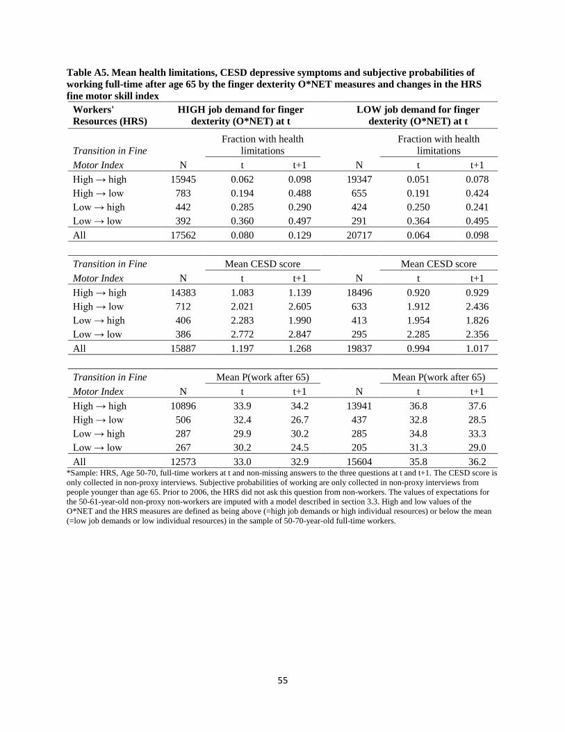
55

Table A5. Mean health limitations, CESD depressive symptoms and subjective probabilities of working full-time after age 65 by the finger dexterity O*NET measures and changes in the HRS fine motor skill index

Workers' Resources (HRS)

HIGH job demand for finger dexterity (O*NET) at t LOW job demand for finger

dexterity (O*NET) at t

Transition in Fine Fraction with health


limitations Motor Index N t t+1 N t t+1 High → high 15945 0.062 0.098 19347 0.051 0.078 High → low 783 0.194 0.488 655 0.191 0.424 Low → high 442 0.285 0.290 424 0.250 0.241 Low → low 392 0.360 0.497 291 0.364 0.495 All 17562 0.080 0.129 20717 0.064 0.098

Transition in Fine Mean CESD score Mean CESD score Motor Index N t t+1 N t t+1 High → high 14383 1.083 1.139 18496 0.920 0.929 High → low 712 2.021 2.605 633 1.912 2.436 Low → high 406 2.283 1.990 413 1.954 1.826 Low → low 386 2.772 2.847 295 2.285 2.356 All 15887 1.197 1.268 19837 0.994 1.017

Transition in Fine Mean P(work after 65) Mean P(work after 65) Motor Index N t t+1 N t t+1 High → high 10896 33.9 34.2 13941 36.8 37.6 High → low 506 32.4 26.7 437 32.8 28.5 Low → high 287 29.9 30.2 285 34.8 33.3 Low → low 267 30.2 24.5 205 31.3 29.0 All 12573 33.0 32.9 15604 35.8 36.2


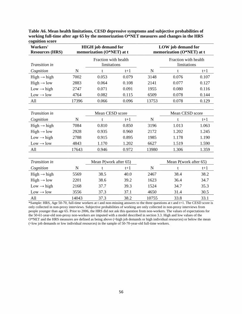
56

Table A6. Mean health limitations, CESD depressive symptoms and subjective probabilities of working full-time after age 65 by the memorization O*NET measures and changes in the HRS cognition score Workers' Resources (HRS)

HIGH job demand for memorization (O*NET) at t LOW job demand for

memorization (O*NET) at t

Transition in Fraction with health


limitations Cognition N t t+1 N t t+1 High → high 7002 0.053 0.079 3148 0.076 0.107 High → low 2883 0.064 0.108 2141 0.077 0.127 Low → high 2747 0.071 0.091 1955 0.080 0.116 Low → low 4764 0.082 0.115 6509 0.078 0.144 All 17396 0.066 0.096 13753 0.078 0.129

Transition in Mean CESD score Mean CESD score Cognition N t t+1 N t t+1 High → high 7084 0.810 0.850 3196 1.013 1.063 High → low 2928 0.935 0.960 2172 1.202 1.245 Low → high 2788 0.915 0.895 1985 1.178 1.190 Low → low 4843 1.170 1.202 6627 1.519 1.590 All 17643 0.946 0.972 13980 1.306 1.359

Transition in Mean P(work after 65) Mean P(work after 65) Cognition N t t+1 N t t+1 High → high 5569 38.5 40.0 2467 38.4 38.2 High → low 2201 38.6 39.2 1623 36.4 34.7 Low → high 2168 37.7 39.3 1524 34.7 35.3 Low → low 3556 37.3 37.1 4650 31.4 30.5 All 14043 37.3 38.2 10755 33.8 33.1


57

Table A7. Mean health limitations, CESD depressive symptoms and subjective probabilities of working full-time after age 65 by the analyzing data or information O*NET measures and changes in the HRS cognition score Workers' Resources (HRS)

HIGH job demand for analyzing data or information (O*NET) at t LOW job demand for analyzing

data or information (O*NET) at t

Transition in Fraction with health


limitations Cognition N t t+1 N t t+1 High → high 6430 0.049 0.073 3720 0.080 0.115 High → low 2515 0.062 0.106 2509 0.077 0.126 Low → high 2360 0.069 0.094 2342 0.080 0.109 Low → low 3763 0.073 0.107 7510 0.083 0.144 All 15068 0.060 0.090 16081 0.081 0.130

Transition in Mean CESD score Mean CESD score Cognition N t t+1 N t t+1 High → high 6502 0.799 0.822 3778 1.001 1.079 High → low 2555 0.931 0.951 2545 1.167 1.212 Low → high 2394 0.911 0.877 2379 1.138 1.160 Low → low 3827 1.131 1.170 7643 1.492 1.554 All 15278 0.922 0.939 16345 1.276 1.334

Transition in Mean P(work after 65) Mean P(work after 65) Cognition N t t+1 N t t+1 High → high 5123 37.9 39.6 2913 39.4 39.2 High → low 1953 38.1 38.2 1871 37.2 36.4 Low → high 1881 37.1 38.3 1811 35.8 37.0 Low → low 2854 36.7 36.5 5352 32.5 31.7 All 12300 36.8 37.6 12498 34.8 34.4


Table A6 shows our analysis for mismatches between cognitive resources and

memorization demands on the job, and Table A7 shows the same analysis for mismatches

between cognitive resources and analytical demands of a job. The patterns are more similar to

the fine-motor skill results in Table A5 than to the large-muscle results in Table A4. Cognitive

58

decline predicts the outcome variables relatively strongly (though less strongly than fine-motor

skills do), but there are only weak interactions with job demands.

For example, among individuals who develop cognitive problems and work in

occupations that demand memorization, the propensity to report work-limiting health problems

increases from 6.4% at t to 10.8% at t+1. Among such workers in occupations that do not

demand memorization, work-limiting health problems increase even more, from 7.7% to 12.7%.

References

Ben-Porath, Yoram. 1967. "The production of human capital and the life cycle of earnings."

Journal of Political Economy 75 (4, Part 1):352-365.

Firpo, Sergio, Nicole Fortin, and Thomas Lemieux. 2011. "Occupational tasks and changes in

the wage structure."

Fraade-Blanar, Laura A, Jeanne M Sears, Kwun Chuen G Chan, Hilaire J Thompson, Paul K

Crane, and Beth E Ebel. 2017. "Relating Older Workers’ Injuries to the Mismatch

Between Physical Ability and Job Demands." Journal of Occupational and

Environmental Medicine 59 (2):212-221.

Grossman, Michael. 1972. "On the concept of health capital and the demand for health." Journal

of Political Economy 80 (2):223-255.

Nolte, Michael A., MA Servais, and M Turf. 2013. "Occupation and industry coding in

HRS/AHEAD." Health and Retirement Study Documentation Report, DR-021.

Roy, Andrew Donald. 1951. "Some thoughts on the distribution of earnings." Oxford Economic

Papers 3 (2):135-146.

Willis, Robert J, and Sherwin Rosen. 1979. "Education and self-selection." Journal of political

Economy 87 (5, Part 2):S7-S36.

59

Appendix B: Additional outcome variables

Table B1. OLS regressions of the change in the subjective probabilities of working full-time after age 62 as a function of job demands, resources and their interactions [1] [2] [3] [4] Large muscle index at t 1.516


[0.294]*** Dynamic strength at t, D1 -0.642

[0.181]*** R1 x D1 0.655

[0.287]** Fine motor index at t 1.451



[0.181]** R2 x D2 0.269 [0.228]

Cognition at t 1.088 1.089 [0.264]*** [0.264]***


Memorization at t, D3 0.384 [0.214]*

R3 x D3 -0.009 [0.287]

Analyzing data or information at t, D4 0.385 [0.205]*

R3 x D4 0.177 [0.284]

Change in age 0.664 0.591 0.429 0.427 [0.717] [0.719] [0.747] [0.747]


Change in age - 50 cube 0.012 0.012 0.009 0.009 [0.005]** [0.005]** [0.005] [0.005]

Change in married -2.184 -2.051 -1.545 -1.539 [1.248]* [1.259] [1.335] [1.336]

Wave dummies Yes Yes Yes Yes Constant -1.350 -1.231 -1.270 -1.278 [1.073] [1.075] [1.097] [1.098]

R-squared 0.008 0.007 0.006 0.006 N 24226 24227 21064 21064

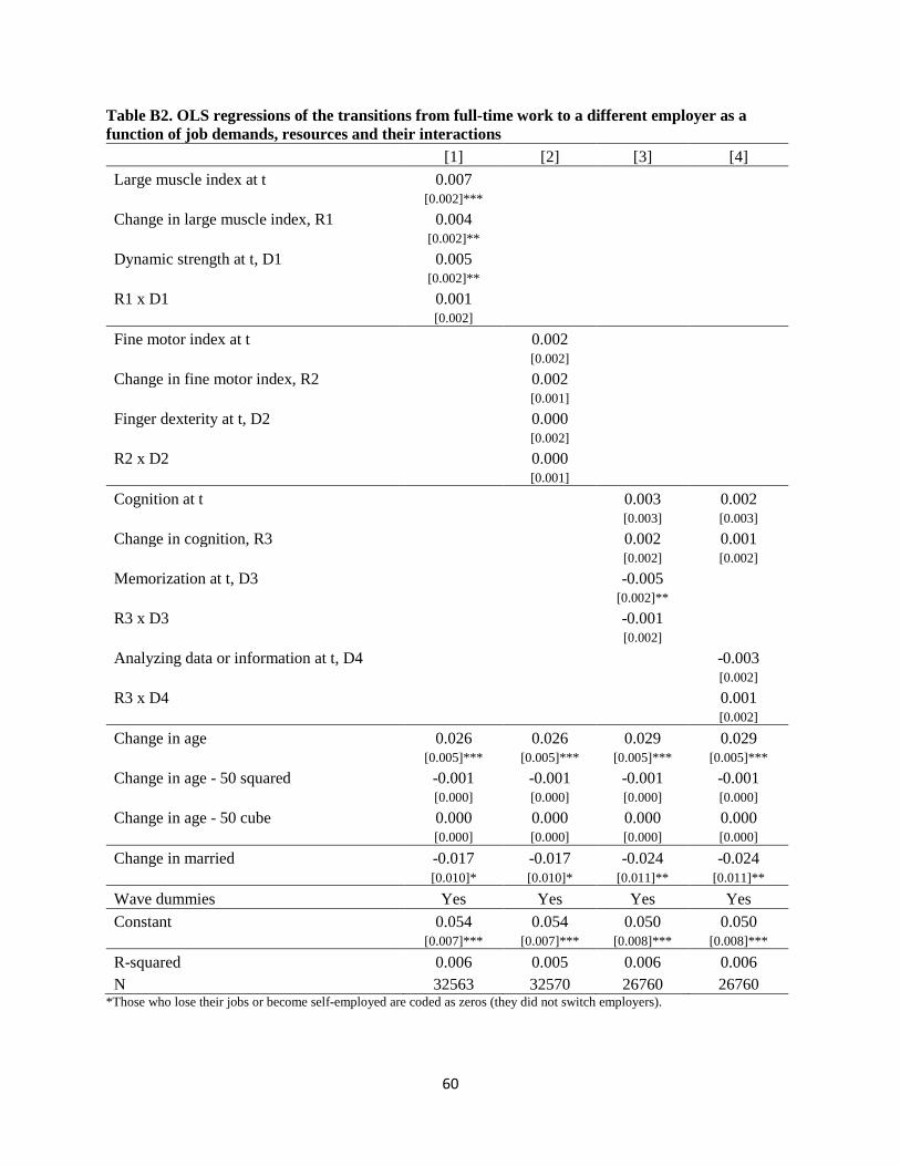
60

Table B2. OLS regressions of the transitions from full-time work to a different employer as a function of job demands, resources and their interactions [1] [2] [3] [4] Large muscle index at t 0.007


[0.002]** Dynamic strength at t, D1 0.005

[0.002]** R1 x D1 0.001

[0.002] Fine motor index at t 0.002

[0.002] Change in fine motor index, R2 0.002

[0.001] Finger dexterity at t, D2 0.000

[0.002] R2 x D2 0.000 [0.001]

Cognition at t 0.003 0.002 [0.003] [0.003]

Change in cognition, R3 0.002 0.001 [0.002] [0.002]

Memorization at t, D3 -0.005 [0.002]**

R3 x D3 -0.001 [0.002]

Analyzing data or information at t, D4 -0.003 [0.002]

R3 x D4 0.001 [0.002]

Change in age 0.026 0.026 0.029 0.029 [0.005]*** [0.005]*** [0.005]*** [0.005]***



Change in married -0.017 -0.017 -0.024 -0.024 [0.010]* [0.010]* [0.011]** [0.011]**


R-squared 0.006 0.005 0.006 0.006 N 32563 32570 26760 26760

*Those who lose their jobs or become self-employed are coded as zeros (they did not switch employers).

61

Table B3. OLS regressions of the change in disliking to work as a function of job demands, resources and their interactions [1] [2] [3] [4] Large muscle index at t -0.001

[0.002] Change in large muscle index, R1 -0.007

[0.003]** Dynamic strength at t, D1 -0.002

[0.002] R1 x D1 0.002


[0.002]* Change in fine motor index, R2 -0.007


[0.001] R2 x D2 0.000 [0.002]

Cognition at t 0.003 0.002 [0.002] [0.002]



R3 x D3 0.000 [0.002]

Analyzing data or information at t, D4 0.002 [0.002]

R3 x D4 0.001 [0.003]

Change in age 0.011 0.011 0.010 0.010 [0.006]* [0.006]* [0.006]* [0.006]*





R-squared 0.001 0.001 0.001 0.001 N 29818 29823 26863 26863

*Disliking to work is defined as disagreeing or strongly disagreeing with the statement that “I really enjoy going to work.”

62

Appendix C: Robustness checks

Table C1. OLS regressions of the change in whether health limits working as a function of job demands, resources and their interactions, using many control variables [1] [2] [3] [4] Large muscle index at t -0.038



[0.002]*** R1 x D1 -0.012




[0.002]* R2 x D2 0.000 [0.002]

Cognition at t -0.007 -0.007 [0.002]*** [0.002]***



R3 x D3 -0.003 [0.002]


R3 x D4 0.001 [0.002]

Female -0.003 0.005 0.009 0.008 [0.003] [0.003]* [0.003]*** [0.003]**

White ref. ref. ref. ref. Black 0.002 0.003 0.003 0.003

[0.004] [0.004] [0.005] [0.005] Other race 0.001 0.004 0.001 0.001

[0.006] [0.006] [0.007] [0.007] Hispanic -0.001 -0.003 0.001 0.001 [0.005] [0.005] [0.006] [0.006]

Less than high school 0.016 0.020 0.022 0.022 [0.005]*** [0.005]*** [0.006]*** [0.006]***

High school ref. ref. ref. ref. Some college 0.005 0.001 0.003 0.003

[0.004] [0.004] [0.004] [0.004]

63

College graduate 0.002 -0.009 -0.009 -0.009 [0.003] [0.003]*** [0.004]** [0.004]**

Change in age -0.019 -0.018 -0.022 -0.022 [0.005]*** [0.005]*** [0.005]*** [0.005]***

Change in age - 50 squared 0.001 0.001 0.001 0.001 [0.000]* [0.000]** [0.000]*** [0.000]***



Change in spouse works 0.001 0.002 0.002 0.002 [0.005] [0.005] [0.005] [0.005]

Change in log household income -0.019 -0.019 -0.021 -0.021 [0.003]*** [0.003]*** [0.003]*** [0.003]***

Change in positive household income -0.010 -0.007 -0.010 -0.010 [0.020] [0.021] [0.023] [0.023]

Change in log household wealth -0.001 -0.001 0.000 0.000 [0.001] [0.001] [0.001] [0.001]

Change in household wealth positive 0.001 -0.003 -0.003 -0.003 [0.022] [0.023] [0.025] [0.025]

Has a DB pension 0.002 0.002 0.003 0.003 [0.004] [0.004] [0.004] [0.004]

Has a DC pension 0.001 -0.001 0.001 0.002 [0.003] [0.003] [0.004] [0.004]

Self-employed -0.005 -0.008 -0.003 -0.003 [0.005] [0.005]* [0.005] [0.005]

Tenure at job, in years 0.000 0.000 0.000 0.000 [0.000]* [0.000]* [0.000]** [0.000]**

Tenure missing 0.013 0.008 -0.008 -0.010 [0.018] [0.019] [0.022] [0.022]

Has health insurance from employer 0.003 0.003 0.005 0.005 [0.004] [0.005] [0.005] [0.005]

Has health insurance from spouse 0.010 0.008 0.012 0.012 [0.005]* [0.005] [0.005]** [0.005]**

Wave dummies Yes Yes Yes Yes Constant 0.047 0.045 0.041 0.041

[0.010]*** [0.010]*** [0.010]*** [0.010]***

R-squared 0.047 0.029 0.010 0.010 N 38272 38279 31149 31149

64

Table C2. OLS regressions of the change in the CESD depressive symptoms as a function of job demands, resources and their interactions, using many control variables [1] [2] [3] [4] Large muscle index at t -0.044



[0.008]** R1 x D1 -0.040




[0.007] R2 x D2 0.004 [0.012]

Cognition at t -0.001 0.000 [0.011] [0.011]



R3 x D3 0.023 [0.012]**


R3 x D4 0.015 [0.012]

Female -0.011 -0.006 0.002 0.001 [0.013] [0.013] [0.014] [0.014]

White ref. ref. ref. ref. Black -0.027 -0.019 -0.023 -0.025

[0.019] [0.019] [0.022] [0.022] Other race 0.015 0.025 0.012 0.012

[0.035] [0.035] [0.038] [0.038] Hispanic -0.036 -0.037 -0.014 -0.015 [0.031] [0.032] [0.033] [0.033]

Less than high school -0.006 0.006 0.040 0.038 [0.023] [0.023] [0.025] [0.025]

High school ref. ref. ref. ref. Some college -0.001 -0.009 0.003 0.005

[0.017] [0.017] [0.018] [0.019] College graduate 0.012 -0.007 -0.005 0.000 [0.017] [0.017] [0.020] [0.019]

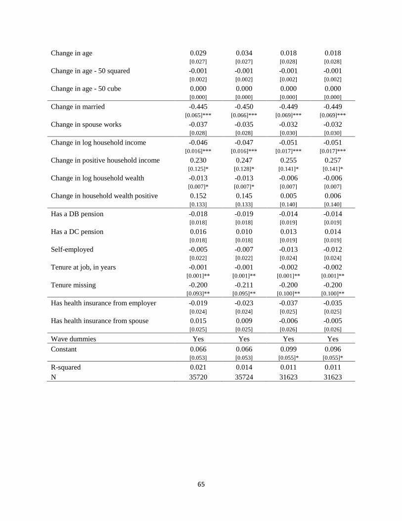
65

Change in age 0.029 0.034 0.018 0.018 [0.027] [0.027] [0.028] [0.028]



Change in married -0.445 -0.450 -0.449 -0.449 [0.065]*** [0.066]*** [0.069]*** [0.069]***

Change in spouse works -0.037 -0.035 -0.032 -0.032 [0.028] [0.028] [0.030] [0.030]


Change in positive household income 0.230 0.247 0.255 0.257 [0.125]* [0.128]* [0.141]* [0.141]*

Change in log household wealth -0.013 -0.013 -0.006 -0.006 [0.007]* [0.007]* [0.007] [0.007]

Change in household wealth positive 0.152 0.145 0.005 0.006 [0.133] [0.133] [0.140] [0.140]

Has a DB pension -0.018 -0.019 -0.014 -0.014 [0.018] [0.018] [0.019] [0.019]

Has a DC pension 0.016 0.010 0.013 0.014 [0.018] [0.018] [0.019] [0.019]

Self-employed -0.005 -0.007 -0.013 -0.012 [0.022] [0.022] [0.024] [0.024]

Tenure at job, in years -0.001 -0.001 -0.002 -0.002 [0.001]** [0.001]** [0.001]** [0.001]**

Tenure missing -0.200 -0.211 -0.200 -0.200 [0.093]** [0.095]** [0.100]** [0.100]**

Has health insurance from employer -0.019 -0.023 -0.037 -0.035 [0.024] [0.024] [0.025] [0.025]

Has health insurance from spouse 0.015 0.009 -0.006 -0.005 [0.025] [0.025] [0.026] [0.026]


[0.053] [0.053] [0.055]* [0.055]*

R-squared 0.021 0.014 0.011 0.011 N 35720 35724 31623 31623

66

Table C3. OLS regressions of the change in the subjective probabilities of working full-time after age 65 as a function of job demands, resources and their interactions, using many control variables [1] [2] [3] [4] Large muscle index at t 1.267



[0.178] R1 x D1 0.802

[0.237]*** Fine motor index at t 1.032



[0.163] R2 x D2 0.112 [0.181]

Cognition at t 0.508 0.492 [0.242]** [0.241]**


Memorization at t, D3 0.302 [0.201]

R3 x D3 -0.215 [0.254]

Analyzing data or information at t, D4 0.414 [0.196]**

R3 x D4 -0.227 [0.246]

Female 0.793 0.525 0.265 0.321 [0.301]*** [0.289]* [0.315] [0.312]


[0.424] [0.424] [0.473] [0.475] Other race -1.024 -1.111 -0.893 -0.893

[0.716] [0.717] [0.743] [0.743] Hispanic 0.952 1.047 1.265 1.292 [0.630] [0.628]* [0.675]* [0.675]*

Less than high school -1.273 -1.421 -1.831 -1.804 [0.498]** [0.493]*** [0.555]*** [0.553]***

High school ref. ref. ref. ref. Some college -0.366 -0.260 -0.672 -0.708

[0.384] [0.382] [0.419] [0.423]* College graduate 0.157 0.552 -0.071 -0.150 [0.389] [0.383] [0.445] [0.439]

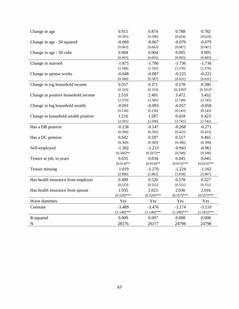
67

Change in age 0.915 0.874 0.788 0.782 [0.595] [0.596] [0.624] [0.624]




Change in spouse works -0.048 -0.087 -0.225 -0.221 [0.588] [0.587] [0.631] [0.631]

Change in log household income 0.357 0.371 0.578 0.580 [0.310] [0.310] [0.330]* [0.331]*

Change in positive household income 2.510 2.491 3.472 3.452 [2.570] [2.583] [2.740] [2.743]

Change in log household wealth -0.091 -0.093 -0.057 -0.058 [0.136] [0.136] [0.143] [0.143]


Has a DB pension -0.158 -0.147 -0.268 -0.271 [0.394] [0.395] [0.423] [0.423]

Has a DC pension 0.542 0.597 0.517 0.465 [0.369] [0.369] [0.396] [0.398]

Self-employed -1.302 -1.213 -0.943 -0.961 [0.566]** [0.567]** [0.598] [0.598]

Tenure at job, in years 0.035 0.034 0.045 0.045 [0.014]** [0.014]** [0.015]*** [0.015]***

Tenure missing -1.019 -1.270 -1.224 -1.162 [2.890] [2.862] [3.058] [3.067]

Has health insurance from employer 0.499 0.520 0.578 0.527 [0.523] [0.525] [0.551] [0.551]

Has health insurance from spouse 1.935 2.021 2.036 2.016 [0.529]*** [0.529]*** [0.557]*** [0.557]***

Wave dummies Yes Yes Yes Yes Constant -3.489 -3.476 -3.174 -3.110

[1.148]*** [1.146]*** [1.180]*** [1.181]***

R-squared 0.009 0.007 0.008 0.008 N 28176 28177 24798 24798

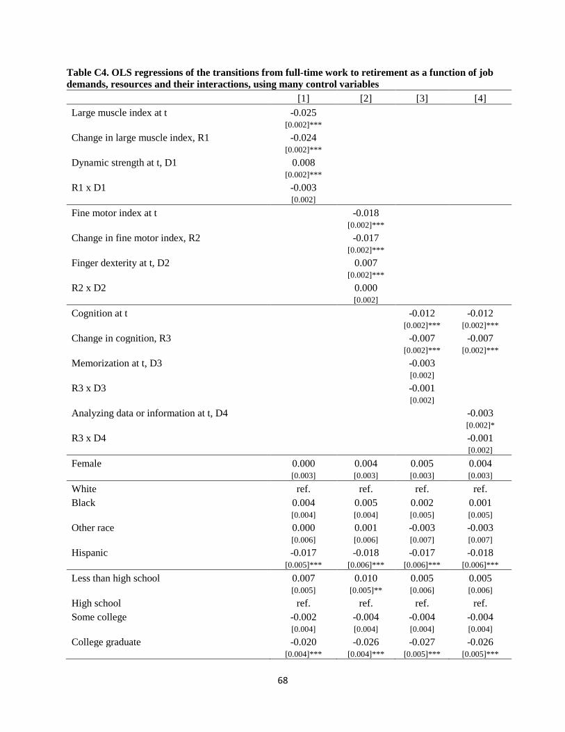
68

Table C4. OLS regressions of the transitions from full-time work to retirement as a function of job demands, resources and their interactions, using many control variables [1] [2] [3] [4] Large muscle index at t -0.025



[0.002]*** R1 x D1 -0.003




[0.002]*** R2 x D2 0.000 [0.002]

Cognition at t -0.012 -0.012 [0.002]*** [0.002]***



R3 x D3 -0.001 [0.002]

Analyzing data or information at t, D4 -0.003 [0.002]*

R3 x D4 -0.001 [0.002]

Female 0.000 0.004 0.005 0.004 [0.003] [0.003] [0.003] [0.003]


[0.004] [0.004] [0.005] [0.005] Other race 0.000 0.001 -0.003 -0.003

[0.006] [0.006] [0.007] [0.007] Hispanic -0.017 -0.018 -0.017 -0.018 [0.005]*** [0.006]*** [0.006]*** [0.006]***

Less than high school 0.007 0.010 0.005 0.005 [0.005] [0.005]** [0.006] [0.006]

High school ref. ref. ref. ref. Some college -0.002 -0.004 -0.004 -0.004

[0.004] [0.004] [0.004] [0.004] College graduate -0.020 -0.026 -0.027 -0.026 [0.004]*** [0.004]*** [0.005]*** [0.005]***

69

Change in age -0.054 -0.055 -0.053 -0.053 [0.004]*** [0.004]*** [0.004]*** [0.004]***

Change in age - 50 squared 0.003 0.003 0.003 0.003 [0.000]*** [0.000]*** [0.000]*** [0.000]***


Change in married 0.033 0.032 0.037 0.037 [0.009]*** [0.009]*** [0.010]*** [0.010]***

Change in spouse works -0.035 -0.035 -0.035 -0.036 [0.005]*** [0.005]*** [0.006]*** [0.006]***


Change in positive household income 0.104 0.104 0.100 0.100 [0.017]*** [0.017]*** [0.019]*** [0.019]***

Change in log household wealth 0.002 0.002 0.002 0.002 [0.001]** [0.001]** [0.001]** [0.001]**

Change in household wealth positive -0.035 -0.035 -0.034 -0.034 [0.015]** [0.015]** [0.016]** [0.016]**

Has a DB pension 0.050 0.050 0.051 0.051 [0.004]*** [0.004]*** [0.004]*** [0.004]***

Has a DC pension -0.008 -0.009 -0.009 -0.008 [0.003]** [0.003]*** [0.004]** [0.004]**

Self-employed -0.045 -0.046 -0.043 -0.043 [0.004]*** [0.004]*** [0.005]*** [0.005]***

Tenure at job, in years 0.002 0.002 0.001 0.001 [0.000]*** [0.000]*** [0.000]*** [0.000]***

Tenure missing 0.030 0.028 0.018 0.017 [0.018]* [0.019] [0.022] [0.022]

Has health insurance from employer 0.000 -0.001 0.000 0.001 [0.004] [0.004] [0.005] [0.005]

Has health insurance from spouse 0.012 0.011 0.012 0.012 [0.005]*** [0.005]** [0.005]** [0.005]**


[0.008]*** [0.008]*** [0.009]*** [0.009]***

R-squared 0.099 0.096 0.092 0.092 N 38829 38838 31645 31645

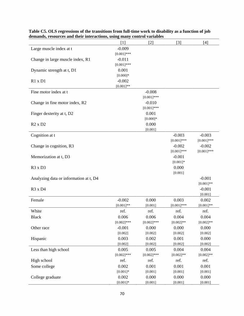
70

Table C5. OLS regressions of the transitions from full-time work to disability as a function of job demands, resources and their interactions, using many control variables [1] [2] [3] [4] Large muscle index at t -0.009



[0.000]* R1 x D1 -0.002

[0.001]** Fine motor index at t -0.008



[0.000]* R2 x D2 0.000 [0.001]

Cognition at t -0.003 -0.003 [0.001]*** [0.001]***


Memorization at t, D3 -0.001 [0.001]*

R3 x D3 0.000 [0.001]


R3 x D4 -0.001 [0.001]

Female -0.002 0.000 0.003 0.002 [0.001]** [0.001] [0.001]*** [0.001]**


[0.002]*** [0.002]*** [0.002]** [0.002]** Other race -0.001 0.000 0.000 0.000

[0.002] [0.002] [0.002] [0.002] Hispanic 0.003 0.002 0.001 0.000 [0.002] [0.002] [0.002] [0.002]

Less than high school 0.005 0.005 0.004 0.004 [0.002]*** [0.002]*** [0.002]** [0.002]**

High school ref. ref. ref. ref. Some college 0.002 0.001 0.001 0.001

[0.001]* [0.001] [0.001] [0.001] College graduate 0.002 0.000 0.000 0.000 [0.001]* [0.001] [0.001] [0.001]

71

Change in age 0.001 0.001 -0.001 -0.001 [0.001] [0.001] [0.001] [0.001]


Change in age - 50 cube 0.000 0.000 0.000 0.000 [0.000] [0.000] [0.000]* [0.000]*


Change in spouse works 0.000 0.000 0.000 0.000 [0.001] [0.001] [0.001] [0.001]


Change in positive household income -0.005 -0.005 -0.002 -0.002 [0.008] [0.008] [0.009] [0.009]

Change in log household wealth 0.000 0.000 0.000 0.000 [0.000] [0.000] [0.000] [0.000]


Has a DB pension -0.002 -0.002 -0.001 -0.001 [0.001]* [0.001]* [0.001] [0.001]

Has a DC pension -0.001 -0.001 0.000 0.000 [0.001] [0.001] [0.001] [0.001]

Self-employed -0.004 -0.004 -0.003 -0.003 [0.001]*** [0.001]*** [0.001]** [0.001]**

Tenure at job, in years 0.000 0.000 0.000 0.000 [0.000]*** [0.000]*** [0.000]*** [0.000]***

Tenure missing 0.001 -0.001 0.004 0.004 [0.006] [0.006] [0.008] [0.008]

Has health insurance from employer -0.003 -0.003 -0.004 -0.004 [0.001]** [0.001]** [0.001]*** [0.001]***

Has health insurance from spouse -0.003 -0.003 -0.003 -0.003 [0.001]** [0.001]** [0.002]** [0.002]*


[0.003]*** [0.003]*** [0.003]*** [0.003]***

R-squared 0.023 0.027 0.008 0.008 N 38829 38838 31645 31645

72

Table C6. OLS regressions of lagged work limiting health problems as a function of job demands, resources and their interactions, balancing tests [1] [2] [3] [4] Large muscle index at t -0.018


[0.002] Dynamic strength at t, D1 0.000

[0.001] R1 x D1 0.002




[0.001] R2 x D2 0.000 [0.002]

Cognition at t 0.001 0.001 [0.002] [0.002]



R3 x D3 0.000 [0.002]


R3 x D4 -0.004 [0.002]**

Change in age 0.008 0.007 0.005 0.005 [0.005] [0.005] [0.006] [0.006]





R-squared 0.006 0.005 0.003 0.003 N 31775 31781 25208 25208

73

Table C7. OLS regressions of lagged CESD depressive symptoms as a function of job demands, resources and their interactions, balancing tests [1] [2] [3] [4] Large muscle index at t -0.057


[0.015] Dynamic strength at t, D1 -0.012

[0.009] R1 x D1 0.006


[0.013] Change in fine motor index, R2 -0.013


[0.012] R2 x D2 0.000 0.000

Cognition at t 0.020 0.020 [0.014] [0.014]



R3 x D3 0.000 0.000


R3 x D4 -0.027 [0.063]

Change in age 0.025 0.023 0.024 0.024 [0.034] [0.034] [0.034] [0.034]





R-squared 0.007 0.006 0.005 0.005 N 25617 25622 25178 25178

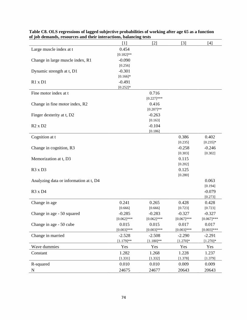
74

Table C8. OLS regressions of lagged subjective probabilities of working after age 65 as a function of job demands, resources and their interactions, balancing tests [1] [2] [3] [4] Large muscle index at t 0.454

[0.182]** Change in large muscle index, R1 -0.090

[0.256] Dynamic strength at t, D1 -0.301

[0.166]* R1 x D1 -0.491

[0.252]* Fine motor index at t 0.716


[0.207]** Finger dexterity at t, D2 -0.263

[0.163] R2 x D2 -0.104 [0.186]

Cognition at t 0.386 0.402 [0.235] [0.235]*

Change in cognition, R3 -0.258 -0.246 [0.303] [0.302]


R3 x D3 0.125 [0.280]


R3 x D4 -0.079 [0.273]

Change in age 0.241 0.265 0.428 0.428 [0.666] [0.666] [0.723] [0.723]

Change in age - 50 squared -0.285 -0.283 -0.327 -0.327 [0.062]*** [0.062]*** [0.067]*** [0.067]***

Change in age - 50 cube 0.015 0.015 0.017 0.017 [0.003]*** [0.003]*** [0.003]*** [0.003]***

Change in married -2.528 -2.508 -2.290 -2.291 [1.179]** [1.180]** [1.270]* [1.270]*

Wave dummies Yes Yes Yes Yes Constant 1.282 1.268 1.228 1.237 [1.331] [1.332] [1.378] [1.379]

R-squared 0.010 0.010 0.009 0.009 N 24675 24677 20643 20643

75

Table C9. OLS regressions of work limiting health problems, CESD depressive symptoms, subjective probabilities of working after age 65, and transitions from full-time work to disability as a function of job demands, resources and their interactions, restricted to full-time workers at t+1

health limitation CESD PW65

Large muscle index at t -0.009 -0.006 0.441 [0.002]*** [0.010] [0.194]**

Change in large muscle index, R1 -0.041 -0.171 1.020 [0.003]*** [0.016]*** [0.293]***

Dynamic strength at t, D1 0.002 0.001 -0.159 [0.001] [0.008] [0.169]

R1 x D1 -0.005 -0.037 0.746 [0.003]* [0.016]** [0.290]**

Change in age -0.014 0.026 0.698 [0.005]*** [0.029] [0.662]

Change in age - 50 squared 0.000 -0.001 -0.205 [0.000] [0.002] [0.070]***

Change in age - 50 cube 0.000 0.000 0.016 [0.000] [0.000] [0.003]***

Change in married -0.004 -0.497 -2.116 [0.010] [0.077]*** [1.361] Wave dummies Yes Yes Yes Constant 0.028 -0.010 -0.555 [0.009]*** [0.051] [1.114] R-squared 0.017 0.017 0.009 N 28950 26903 22043

the effect of physical and cognitive decline at older ages

Documents