the effect of non-ventilated plate- cavity devices on...
TRANSCRIPT

THE EFFECT OF NON-VENTILATED PLATE-
CAVITY DEVICES ON DRAG REDUCTION
OF TRACTOR-TRAILERS
J. D. Coon
K. D. Visser
Department of Mechanical and Aeronautical Engineering
Clarkson University
Potsdam, NY
13699-5725
Report No. MAE-361
June 2002
Final Report
Contract Grant Agreement #6436 Trailer Drag Reduction
The New York State Energy Research and Development Authority

The following report is submitted to The New York State Energy Research and
Development Authority (NYSERDA) in fulfillment of Contract Agreement # 6436. This
work represents a thesis submitted by Jamison Coon, in partial fulfillment of the
requirements for the degree of Master of Science in Mechanical Engineering, and
accepted by the Graduate School of Clarkson University, Potsdam, NY 13699.
The report is supplemented by a copy of the paper “Aft-end drag reduction of tractor-
trailers” in submission to the SAE Journal of Automobile Engineering.
A CD-ROM accompanies this report and contains the data acquired to date, e-copies of
this documentation and several electronic slide presentations.
Questions pertaining to this work can be directed to the address below.
Dr. Kenneth D. Visser
Department of Mechanical and Aeronautical Engineering
Clarkson University
P.O. Box 5725, Potsdam, New York, 13699-5725
Tel: 315 268 7687 Fax: 315 268 6438
June 2002

Executive Summary
An experimental and numerical study has been conducted to examine the effectiveness
and feasibility of drag reduction using a wide variety of unventilated cavity devices on
the aft face of tractor-trailers. The performance of the proposed drag reduction devices
was evaluated using a 1:15 scale model of a Peterbilt 379 tractor and 48 foot trailer.
Numerical simulation, using indicated the design would reduce the pressure drag on the
aft face of the trailer. Scale model drag increments obtained in the Clarkson University
subsonic wind tunnel indicated a drag reduction of up to 9% of the isolated trailer drag.
Effects of yaw angle, up to 9 degress off axis, were also examined
A full scale prototype design was constructed based on predicted performance as well as
practicality, and ease of manufacture. Cross-country road data indicated a drag savings
which, when converted to a fuel savings, would save on the order of 1500 gallons of fuel
per year per truck. This corresponds to about an 8% fuel savings based on standard
yearly driving distances. A second generation full scale aluminum prototype was also
designed and road tested with inconclusive results.

Contents
Abstract iii
Acknowledgements iv
Table of Contents v
List of Figures vii
Nomenclature ix
Chapter 1: Introduction 1
1.1 Overview 1
1.2 Background 2
1.2.1 Increased Flow Attachment 3
1.2.2 Controlled Flow Separation 5
1.2.3 Non-Ventilated Cavity and Boattail Comparison 12
1.2.4 Application to Full-Scale 14
1.3 Current Objectives 15
Chapter 2: Computational Study 17
2.1 Computational Model 17
2.1.1 Model Description 17
2.1.2 Conditions 20
2.1.3 Parametric Study 21
2.2 Procedure 23
Chapter 3: Experimental Setup 25
3.1 Wind Tunnel 25
3.1.1 Wind Tunnel Model 25
3.1.2 Modeled Ground Plane 27
3.1.3 Plate Device Construction 29
3.2 Biaxial Force Balance 31
3.3 Other Instrumentation 33
3.4 Data Acquisition 34
Chapter 4: Experimental Procedure 36
4.1 Calibration 36

4.2 Testing 38
4.2.1 Zero Degree Yaw Testing 38
4.2.2 Yaw Angle Testing 40
4.3 Models Tested 40
4.3.1 Parametric Study 40
4.3.2 Angled Plate Study 43
Chapter 5: Results 46
5.1 Computational Results 47
5.1.1 Pressure Drag Calculations 47
5.1.2 Momentum Drag Calculations 49
5.1.3 Slip Condition Implementation 50
5.1.4 Matched Reynolds Number 51
5.1.5 Computational Assumptions and Error 51
5.2 Wind Tunnel Results 52
5.2.1 Zero Degree Yaw Test Results 52
5.2.1.1 Equal Inset 52
5.2.1.2 Effect of Zero Bottom Plate Inset 53
5.2.1.3 Effect of Top Plate Removal 55
5.2.1.4 Shift in Optimums 57
5.2.2 Yaw Test Results 58
5.2.2.1 Plate Cavity Designs 58
5.2.2.2 Angled Plate Designs 61
5.2.3 Wind Tunnel Error Estimates 64
5.3 Results Comparison 65
5.3.1 Computational/Experimental Results 65
5.3.2 Comparison to Previous Work 67
Chapter 6: Conclusions and Recommendations 71
6.1 Conclusions 71
6.2 Recommendations for Future Study 75
Appendix A – 76
Bibliography 84

1
Chapter 1: Introduction
The flow around a tractor-trailer can be described as a complex flow around a bluff body.
This body experiences a large base drag due to its shape, as the sharp trailer corners and
the flat back face of the trailer cause the flow to separate from the trailing edges. The
flow behavior is similar to that of a pump, in that the separated air that leaves the trailer
edges tries to pump away the stagnant air at the base of the trailer [1]. The primary effect
is a decrease in static pressure at the base of the trailer. This base pressure is largely
dependent upon the length of the tractor-trailer, and its surface conditions. This decrease
in static pressure at the base of the trailer causes a pressure drag on the vehicle that
contributes a large portion to the overall drag [2].
The average Class 8 heavy-duty tractor-trailer, weighing about 80,000 pounds, has a drag
coefficient of roughly CD=0.6. At 70mph, about 65% of the total energy used by a
typical truck is due to the aerodynamic drag [3]. Reducing the aerodynamic drag by a
small percentage through the re-shaping of the tractor, trailer, or both will have a
significant effect on the fuel consumption.
1.1 Background
Millions of Class 8 tractor-trailers are in operation all around the world. They contribute
to a large consumption of fuel, as well as pollution, in an era of environmental concern.

2
The streamlining of tractor-trailers will decrease their fuel consumption, and as a direct
result, will decrease the amount of particulates emitted to the atmosphere every year.
Extensive work has been done to alter the front of the tractor-trailer with items such as
cab fairings and cab/trailer gap fairings. There is, however, much room for aerodynamic
improvement at the trailer base of many common tractor-trailers, such as the one seen in
Fig.1.1.
Many methods have been suggested and experimentally tested that involve altering the
trailer base or the addition of base attachments to reduce the base pressure drag. These
modifications can be broken down into two categories: those designed to increase flow
attachment and those designed to control the flow separation location. The following
section gives a brief review.
1.1.1 Increased Flow Attachment
The flow separation that occurs at the trailing edges of the trailer in conjunction with the
blunt shape of the trailer base contributes greatly to the base pressure drag. The drag on
the tractor-trailer may be reduced by decreasing the amount of separation that occurs off
Figure 1.1 Common Tractor-Trailer

3
the trailing edges of the trailer. This will narrow the size of the wake aft of the trailer
base. Both active and passive methods for increased flow attachment are discussed
below.
The addition of a boattail that rounds the back end of the trailer can minimize separation
at the trailer’s sharp corners. A boattail may be described as a smooth, rounded convex
shape that may or may not come to a distinct point. With the correct shape, the flow
should follow the contour of the boattail and keep the flow attached further downstream
on the overall trailer shape (Fig. 1.2a). Boattail concepts have been patented by
researchers such as Lechner, Keedy, Davis, and Mulholland. [4,5,6,7]. Many of these
patents utilize the same idea with minor differences in geometry, deployment, and
compaction methods.
Research performed at NASA deduced that the boattail may be truncated (Fig.1.2c), and
still achieve nearly as much drag savings as in the non-truncated case [8,9,10]. For
example, Muirhead [10] performed wind tunnel experiments on boattail shapes that
extend to a point (Fig. 1.2b). The boattail tested was given a specific radius of curvature
to trailer width ratio. The tests were then repeated with a truncated version of the boattail
(Fig. 1.2c). The truncated boattail was created by chopping the end off of the pointed
boattail. This was done to satisfy legal concerns involving maximum allowable lengths
for rear attachments on tractor-trailers. The full length of the non-truncated boattail will
be above the legal limit for length of a tractor-trailer attachment length.

4
Full-scale tests of truncated and non-truncated boattails were conducted as well by
Peterson [8]. A flow visualization analysis was performed on both boattail variations.
The tests concluded that separation in the flow was being delayed due to the addition of
the device. This can be attributed to the curvature in the boattail. The truncated boattail
in this experiment also displayed similar results.
Active flow methods have also been proposed to reduce drag. One example involves
injecting air into the low pressure region at the base. This method would cause the base
pressure to increase and thus reduce the pressure drag acting at the back of the truck. An
example of such a study by Sykes, described in [11], concluded that the injecting of air
(a.)
(b.)
(c.)
Figure 1.2 Examples of Drag Reducing Boattail Extensions on Tractor-Trailers (a.) rounded boattail
extension (b.) curved boattail extension that comes to a point (c.) truncated version of (b.)

5
into the base region of a bluff body works, but is not economical. The power required to
inject air into the base region is impractical when compared to the savings in drag.
Work currently being conducted at Georgia Tech includes the blowing of compressed air
from slots located on the top, sides, and bottom of the trailer [12]. The airflow is
smoothed by the air being injected into the free-stream from different locations along the
trailer’s length. Researchers at Georgia Tech claim that a 35% decrease in aerodynamic
drag may be achieved through this drag reduction method.
1.1.2 Controlled Flow Separation
Many passive flow control methods have been suggested to reduce the pressure drag on a
tractor-trailer including splitters, vanes, cavities, and plate designs. These ideas involve
the controlling of separated flow. By allowing the flow to separate along the sharp
corners at the base of the trailer as it would normally, it can be manipulated passively
downstream of the trailer base into a number of controlled vortex formations with altered
trailer base geometry.
In 1976, Mason and Beebe [13] conducted wind tunnel experiments on a 1/7 scale truck
model with Re=2*106, based on the effective diameter of the truck, dEFF, calculated using
the cross-sectional area of the model.
2/1)/4( !AdEFF
"= (1)
Devices such as vertical and horizontal splitters, vanes, and cavities, as pictured in Fig.
1.3, were added to the base of the trailer.

6
The vertical and horizontal splitters (Fig.1.3a) are plates mounted perpendicular to the
trailer base and extend rearward. In this method the flow is allowed to separate off the
trailing edges of the trailer. The devices attempt to trap vortex structures between the
plate and the base of the trailer, however, no significant change in drag coefficient was
observed. The vanes Mason and Beebe tested (Fig.1.3b), which were implemented in
hopes of directing the flow inward towards the region of lower pressure air, actually
added drag in their tests.
The non-ventilated cavity design (Fig.1.3c) proved to be the most beneficial, with a !CD
of 0.03. The device used had a depth of 0.13*dEFF (Eq.1). It was assumed that the
estimated reduction in drag of 5% was attributed to the increase in base pressure inside
the cavity due to the vortices being shed off the trailing edges of the cavity walls.
Figure 1.3 Trailer Devices Tested by Mason and Beebe [13]
(a.) Vertical and Horizontal Splitters (b.) Vanes (c.) Cavities
(a.)
(c.) (b.)

7
Similar research by Hucho [14] in the late 1970s also proved the capabilities of non-
ventilated cavities. He examined the effects on small minivan style vehicles with equally
promising results. The device consists of a 4-plate cavity design, each plate flush with
the top, sides, and bottom of the trailer. Figure 1.4 shows the device tested by Hucho and
the results for the small van experiments. The results indicate a drag reduction of
approximately 6% with a plate length to van length ratio of about 0.22.
In 1987, a patent was filed by Bilanin [11], for a four-sided non-ventilated cavity design
with a very specific plate-cavity geometry (Fig.1.5). The device has characteristics
similar to both the cavity and splitter devices tested by Mason and Beebe (Fig.1.3a,c).
The Bilanin device includes four plates oriented in a box formation. Note that three of
the plates (top and sides) are inset from the perimeter of the trailer base and that the
bottom plate has no inset and is in line with the bottom of the trailer. All plates are
mounted perpendicular to the trailer base.
Figure 1.4 Hucho Add-on Device and Results [14]

8
Since three of the plates are inset from the perimeter of the trailer base, the flow will still
separate at the trailing edges of the trailer. This orientation of plates produces vortex
structures in the area between the plate and the perimeter of the trailer. Recall that this
was the intent of the Mason and Beebe splitter devices (Fig.1.3a). Figure 1.6 illustrates
the flow around the trailer base with the addition of the Bilanin plate-cavity device (top
view).
Figure 1.6 Controlled Vortex Formation with Plate Implementation (Top View)
Figure 1.5 Bilanin Patent Plate Design [11]
TRAILER BASE
PLATE DEVICE
D
W
L

9
The captured vortices turn the flow inward and effectively reduce the base area of the
trailer, thereby reducing the drag. The base pressure is increased and the drag is
decreased. The flow also separates once again at the trailing edges of the plates. It is
conceivable that some of this separated flow curls around the plates and stagnates inside
the cavity region, possibly contributing to the increase in base pressure.
The optimum dimensions reported in the Bilanin publication, illustrated in Figures 1.6
and 1.7, were:
D/W=0.13, G/H=0.15, D/L=G/L=0.3
where D = plate inset from each of the sides of the trailer
G = plate inset from the top of the trailer
W = width of trailer;
H = height of trailer;
L = plate length
G
H
D
L
W
Figure 1.7 Dimensions for Bilanin Device [11] (trailer base view)

10
With these criteria, Bilanin claims that a 10.2% reduction in drag was achieved on a
typical tractor-trailer with a base tractor-trailer CD of 0.6, however no test results have
been published in the literature. Bilanin includes optimum ranges for the geometric ratios
previously specified, in order to adjust for maximum efficiency of vortex capture and for
structural members already existing on the trailer base. These ratio ranges are:
0.1"D/W"0.2, 0.1"G/H"0.2, 0.2"D/L=G/L"0.4
Bilanin also specifies that the length of the plates should be between 40” and 56”.
Lanser and Ross [15] performed tests in conjunction with Kaufman from Continuum
Dynamics in 1988, expanding upon the patent data reported by Bilanin. Full-scale tests
were conducted on a plate-cavity extension, similar to that of Bilanin [11], in the
80’x120’ wind tunnel facility at the NASA Ames Research Center, California. Figure 1.8
shows the full-scale experimental setup.
Figure 1.8 Experimental Setup of Lanser, et al [15]

11
The model consisted of a Navistar International Transportation Corporation 9700 cab and
a Fruehauf Corporation 48 foot trailer. A total of 241 pressure taps were mounted on the
aft face of the trailer to measure the pressure distribution. Most of the tests were
performed at a dynamic pressure of 8.4 lbs/ft2, or 58mph, over a yaw range of –15° to
+15°. A total of 17 configurations were tested, with several parameters being varied,
including the plate inset from the top, G, the plate inset from the sides, D, and the plate
length, L (refer to Fig.1.7). All plates were mounted perpendicular to the trailer base as
in the Bilanin patented device.
A complete summary of all geometries tested can be seen in Table 1.1. This shows that
Lanser, et al tested a wide range of plate lengths and insets. The plate length to trailer
width ratio, L/W, ranged from 0 to 0.44; the vertical plate inset ratio, G/W, ranged from 0
to 0.15; and the horizontal plate inset ratio, D/W, ranged from 0 to 0.15.
Table 1.1 Summary of Plate Geometries Tested by Lanser, et al [15]
(optimum highlighted)
L/W G/W D/W
0 0 0
0.24 0.04 0.04
0.24 0.06 0.06
0.24 0.12 0.12
0.3 0.04 0.04
0.3 0.06 0.06
0.3 0.09 0.09
0.3 0.04 0.06
0.3 0.06 0.09
0.36 0.04 0.04
0.36 0.06 0.06
0.36 0.12 0.12
0.36 0.15 0.15
0.36 0.04 0.06
0.44 0.04 0.04
0.44 0.06 0.06
0.44 0.09 0.09

12
The optimum measured values observed in these experiments, at the zero degree yaw
angle, were plate inset ratio G/W=D/W=0.06 and plate length ratio L/W=0.36. All values
are non-dimensionalized by dividing by the width of the trailer.
The trailer data under the yawed conditions indicated that there was greater change in
drag for the higher yaw cases than for the zero yaw condition. The optimum device
reduced drag by at least 10% over the entire range of yaw angles.
A summary table of literature optimum geometries for Bilanin[11], Lanser, et al [15], and
Mason and Beebe [13] can be seen in Table 1.2.
More recently, a company called MAKA Innovation, based in Quebec, Canada, has been
marketing and selling a patented drag-reducing device that utilizes angled plates [16,17].
Their design is different from the previously discussed plate-cavity devices in that it only
uses three plates oriented at a 16° angle inwards from a line normal to the trailer face.
Figure 1.9 shows that there is no inset from the trailer perimeter for any of the three
plates, which are each 20-24 inches long [18]. Also, the device does not have a bottom
plate.
Table 1.2 Summary of Published Optimum Geometries for Plate-Cavity Devices
Publication Geometric Optimums (non-dimensionalized by trailer width)
Lanser, Ross, Kaufman 1991 [15] L/W=0.36; G/W=0.06; D/W=0.06 (see fig.1.7)
Bilanin 1987 [11] L/W=0.44; G/W=0.13; D/W=0.13 (see fig.1.7)
Mason, Beebe 1976 [13] L/W=0.13*dEFF/W (see eq.1)

13
This device attempts to narrow the wake of the tractor-trailer by passively coercing the
flow inward of the trailing edge of the trailer perimeter, in a similar manner as do the
boattails previously mentioned. It does not attempt to trap vortices since there is no plate
inset. The flow is allowed to separate at the trailing edges of the plates. In this manner it
is similar to the aforementioned plate-cavity devices. The separated flow off the plates
may also assist in the pressure increase at the base of the trailer, thus helping to reduce
drag.
1.1.3 Non-Ventilated Cavity and Boattail Comparison
Little research has been performed on both non-ventilated cavities and boattail extensions
in the same experimental set. Kentfield [19] showed a simplified comparison of the two
concepts in 1984. The focus of his work consisted of an analysis of base drag
calculations on short, multi-stepped afterbody fairings. Kentfield’s model was
cylindrical, with a blunt base. He compared this to a model with a long conical shape
placed at the base, as well as a model with a short conical base. He also compared the
blunt base model to a model with steps on the aft face of the cylinder. The steps were
Figure 1.9 MAKA Angled Plate Design [16]

14
concentrically staged at the base of the cylindrical shape. The model shapes are depicted
in Fig.1.10.
The data indicated that the addition of a long conical afterbody decreased the drag
substantially, while the addition of a short cone actually increased the drag in Kentfield’s
experiments, emphasizing the importance on length or cone angle for device
performance. In this experiment, the conical afterbodies most closely represent the
boattail extensions mentioned previously, since they have some slope to their shape
(Fig.1.10b,c). The closest representation to the non-ventilated cavity is the multi-stepped
afterbody fairing (Fig.1.10d). This works in a similar manner in that it forces separated
flow to turn inward, thereby reducing the effective base area. One point worth noting is
(a.)
(d.)
(c.)
(b.)
Figure 1.10 Kentfield Base Drag Models [19] (side profiles)
(a.) blunt base (b.) short conical base (c.) long conical base (d.) multi-stepped base

15
that the stepped afterbody is the same length as is the short conical afterbody (Fig.1.10b),
however, yields much better results. In fact, in terms of drag reduction, the stepped
afterbody comes close to the long conical afterbody, and is one-third its length. The
results may be seen in Table 1.2.
This research merits work on a stepped afterbody in conjunction with a bluff forebody. It
hints that a stepped shape of some sort may provide similar results as a convex extension.
1.1.4 Application to Full-Scale
The focus on plate-cavity designs stems more from practical reasons that lie in the real-
world application of such a device. A cavity design made up of some configuration of
plates is easier to compact when not in use, maximizing trailer accessibility. The device
when applied to full-scale will be simple to manufacture since it contains flat plates that
are easy to construct and requires less construction material than a convex boattail
extension does. Plate-cavity devices are also easy to operate and do not hinder access to
the trailer. A boattail extension may be difficult to collapse or get out of the way of the
doors in order to unload cargo. The cavity design is a more practical solution since it can
be compacted and folded away more easily so that full trailer functionality is maintained.
Table 1.3 Kentfield Base Drag Results [19]
Length/diam. Ratio CD
Afterbody (based on max.
Model Configuration Figure Overall Only cross-sect. area)
blunt base 1.10a 3.250 0.0 0.20
short conical base 1.10b 3.916 0.666 0.23
long conical base 1.10c 5.250 2.000 0.06
multi-stepped base 1.10d 3.916 0.666 0.08

16
1.2 Current Objectives
The current research focused primarily on the use of non-ventilated plate-cavity devices
to reduce the base drag on a tractor-trailer. There are many viable means to reduce the
base drag of a tractor-trailer, however, the plate-cavity designs remain the most practical.
Previous experiments performed on this idea indicate that many design variations have
yet to be tested, such as variation in the number of plates. It is worthwhile to develop a
relative importance for each component on the performance of the device. Also, perhaps
it is better to angle plates and form some plate configuration that way. A variation of
number of plates is performed with the angled plate cases as well.
The present study was comprised of an experimental wind tunnel study, complemented
with a numerical study. Both studies included a parametric study of plate designs with
varying geometries. The objective of the numerical study was to provide direction for the
experimental study. This helped in narrowing down a set of plate configurations that
perform best. It also assisted in visualizing and understanding the flow around a tractor-
trailer, particularly the wake. The objectives of the parametric wind tunnel study were to
find an optimum plate configuration and geometry, and to explain the importance of the
specific components in the plate-cavity design. Both the simulated and wind tunnel
parametric studies had the truck oriented at 0° yaw.
A small set of tests were also run in the wind tunnel for certain plate configurations over
a yaw range of –3° to +9°, in increments of 3°. The objective was to see if the most
promising plate configurations that performed best under the 0° yaw condition performed

17
as well under varied yaw angles. Finally, a small set of angled plate devices were tested
at varying degrees of yaw. A comparison is made between the effect of angled plates and
the effect of plates normal to the trailer base.

18
Chapter 2: Numerical Study
A simulated three-dimensional truck study was performed using the computational fluid
dynamics (CFD) code Fluent. This was used to qualitatively, as well as quantitatively,
assess the use of plates at the aft end of a tractor-trailer for the purpose of drag reduction
on the configuration. The CFD code was used to test many different four-plate
configurations with varying geometries. It should be emphasized that the primary
objective of the numerical study was to provide direction for the experimental wind
tunnel study.
2.1 Numerical Model
2.1.1 Model Description
Since Fluent is an internal fluid dynamics code, the CFD model was constructed by
creating a simulated “wind tunnel” with walls far away from the truck model. The tunnel
created has a cross-section 50x50 ft.2
and length of 150 ft., with the truck placed in the
center of the cross-section. The cab, trailer, and wheels were all included in the model, as
seen in Fig.2.1.

19
The grid spacing close to and including the truck was one foot. Towards the aft end of
the truck, the grid spacing was reduced to a half-foot in order to vary the plate devices
accordingly. There was a limit as to how many total grid points could be used, due to
computer capabilities. In order to alleviate computational time, the grid spacing was
increased to 2 feet far away from the truck. Doing this facilitated the ability for the walls
to be moved further away from the truck, since there were more grid points available.
This helped reduce any possible interference the flow around the truck would experience
due to the walls of the simulated tunnel. The grid spacing and model placement in the
center of the wind tunnel (Fig. 2.2a - front view) show the refined grid spacing close to
and including the truck model. The side view of the grid spacing may be seen in Fig.
2.2b. This illustrates the refined grid spacing around the truck model, particularly at the
Figure 2.1 Fluent Truck Model in Simulated Tunnel (isometric view)

20
base. The model was placed closer to the inlet of the tunnel, rather than the outlet, in
order to allow for more room for flow development (Fig. 2.2b).
A total of 2.64*105 nodes were present in the numerical truck model. A similar study
performed recently at Sandia National Laboratories included similar calculations on a
truck model through CFD [3]. Their model utilized the RANS (Reynolds Averaged
Navier-Stokes) equations and contained a range from 5*105 to 32*10
6 nodes. Their most
(a.)
(b.)
Figure 2.2 Numerical Model Grid Spacing and Model Placement (a.) Front View (b.) Side View

21
coarse model, with 5*105 nodes, contains more nodes than the present model, however,
Sandia National Laboratories used 107 processors in series for their least expensive
calculations, whereas the present study utilized only one processor.
The truck modeled in Fluent was given a width of 8 ft. and a height of 12 ft. The length
dimensions given the model were a cab length of 14 ft., a cab-trailer gap of 3 ft., and a
trailer length of 48 ft., giving a total overall length of 65 ft. As previously stated, the
resolution was increased towards the back of the trailer to enable more variation in the
four-plate configurations tested (Fig.2.2b).
2.1.2 Conditions
The wind tunnel inlet velocity was set at a constant 26 m/s (~55mph), oriented at a zero
degree yaw angle. This particular velocity was chosen since it is a representative
highway speed. The Reynolds number was Re=4.32*106 based on maximum trailer
width and the simulated tunnel blockage was 3.84%.
Fluent uses the RANS equations to numerically solve the flow field around an object,
given a set of conditions. The RANS Equations require a turbulence model for closure,
the most commonly used model being the k-! model, which is widely used in many
commercial applications. In this model, the Reynolds stresses are related to the mean
flow in Equation 2,
ij
j
it
i
j
j
itijji
x
u
x
u
x
ukuu !µµ!""
#
#+$$
%
&
''
(
)
#
#+
#
#*=
3
2
3
2'' (2)
where k represents the turbulent kinetic energy and ut represents the turbulent viscosity,
which is calculated from both a velocity scale, k1/2
, and a length scale, (k1/2
)/! [20]. The

22
scales are predicted at each node in the flow through the use of the transport equations for
k and the dissipation rate, !, shown in Equations 3 and 4,
!"#
µ!! $++
%
%
%
%=
%
%+
%
%bk
ik
t
i
i
i
GGx
k
xku
xk
t)()( (3)
( )( )k
CGCGk
Cxx
uxt
bk
i
t
i
i
i
2
231 1)()(!
"!!
#
µ!""! !!!
!
$$++%
%
%
%=
%
%+
%
% (4)
where Gk is the generation of turbulent kinetic energy and Gb is the generation due to
buoyancy. C1!, C2!, C3!, Cµ, !k, and !! are empirical constants which have derived values.
The k-! turbulence model is a semi-empirical model that provides accuracy for many
applications where turbulent flows exist. This particular model was chosen because of its
common use in industry and its ability to solve a wide variety of turbulent flows.
However, according to the Fluent User’s Manual [20], the k-! model is not well suited for
flows where there exists highly non-isotropic turbulence, such as in swirling flows. The
tractor-trailer example contains swirling flows in its flow field, most notably at the trailer
base. Perhaps a more suitable model could have been used to account for the highly
swirling flows that exist in the trailer wake, such as the Renormalization Group (RNG)
turbulence model. This model yields more accurate results in comparison to the k-!
model for a number of different flows, most especially swirling flows [20]. The
turbulence intensity for the k-! model was set at the default value of 10%.
The simulated tunnel walls were given no-slip wall conditions. It was decided after the
cases were run that this was the incorrect wall condition to model a real-life situation.
The walls should have been given slip conditions, so as to allow for free motion along the
plane of the walls. This is of greatest concern for the area underneath the trailer. The

23
lack of this condition will be discussed later on in the numerical results discussion in
chapter 5.
2.1.3 Parametric Study
The parameters varied in this study included the plate length, L, aft of the trailer and the
plate inset, d, from the perimeter of the trailer. The plate lengths tested were 3, 4, 5, and
6 feet. The plate insets from the perimeter were kept equal from the top, bottom, and
sides of the trailer and varied from 0<d<36 inches in increments of six inches. All plates
are perpendicular to the trailer face. Fig. 2.3 shows a schematic that displays the
parameters varied in the plate cavity study.
The study was simplified in this way to give a better idea of what range to focus on when
approaching the wind tunnel experiment. A total of approximately 40 different
configurations were tested, each computation taking about two to three hours to
converge.
L
d
d
Figure 2.3 Schematic of Plate Cavity Geometry Parameters Varied in Numerical Study

24
Computational resources limited the geometry resolution. Each plate had a thickness of
one grid space, or 6 inches. Prediction of separated flows, such as the one in the tractor-
trailer model, is difficult at best. Since the plates have a thickness of only one grid space,
this makes it even more difficult to resolve. A similar problem with the grid spacing
occurs with the inset of the plates, d, which varied in increments of 6 inches. There are
instances when the plate inset is only one grid space, which causes a problem similar to
that of the plate thickness. This makes it difficult for the program make accurate
calculations involving the supposed vortex formation between the inset and plate. An
example of grid spacing for a device on the base of the truck model may be seen in Fig.
2.4, which illustrates a back view of the trailer. This example in particular has a plate
inset of 6 inches, equivalent to one grid spacing.
2.2 Procedure
The fore-body of the truck was kept constant for all simulated runs. The only change
made for each of the cases run was the geometry of the cavity design. The drag on the
trailer was calculated for all truck geometries. Two calculation methods are discussed.
Figure 2.4 Numerical Grid Spacing for Plate-Cavity Device (Back View)

25
2.2.1 Pressure Drag Calculation Method
Surface pressure results were evaluated for each exposed frontal and rear surface. Each
surface area A, both front and rear, was multiplied by its respective static pressure P.
Drag was then expressed as the difference in the sum of the pressure forces acting along
each surface, as described in Equation 5.
rear
n
j
jjfront
m
i
iiD APAPF )()( !! "= (5)
This method estimated the performance of the geometries tested, without extensive
computation. However, there exists a substantial amount of error in this method, as will
be described later.
The drag results from the CFD study were then plotted using MATLAB. The code, as
seen in Appendix A, constructs a 2-dimensional contour plot from the drag data, with
plate inset on the horizontal axis and plate length on the vertical axis. It also constructs
an interpolated contour plot, which offers a different picture of the drag reduction trends
through the use of color. This plot interpolates additional points in between the actual
points. It offers information that can establish a range for both plate inset and plate
length that provides optimum performance.
2.2.2 Momentum Drag Calculation Method
A second drag calculation method was used to compare to the pressure drag calculation
method. The total momentum was calculated for both the inlet and outlet of the
simulated wind tunnel in CFD. The difference in the momentum flux from the inlet to
the outlet is the drag on the tractor-trailer, as displayed in Equation 6.

26
outletinletoutletfluxinletfluxD dAPudAPuMMF )()( 22
__ +!+=!= "" ## (6)
Equation 6 is derived from the Navier-Stokes equation in closed volume form. The
simplified equation ignores viscous effects at the boundaries and assumes a rectangular
box for a control volume. Results from the CFD cases will be presented in Chapter 5.

27
Chapter 3: Experimental Setup
3.1 Wind Tunnel
Experiments were performed in the Clarkson University indraft, open circuit, subsonic
wind tunnel facility (Fig.3.1). The test section of the tunnel has a cross-section of
1220mm by 910mm (48in. by 36in.), and a length of 1650mm (65in). The tunnel’s inlet
contraction ratio is 4.67:1. The maximum velocity the tunnel achieved for the tests was
approximately 48mph (~21.5m/s). This corresponds to a Re/m of 1.4e06/m.
3.1.1 Wind Tunnel Model
The wind tunnel model was a 1:15.25 scale model that resembles many of the common
tractor-trailers on the road today (Fig.3.2). The cab was modeled after a Peterbilt tractor
model 579 and the trailer was modeled after a standard full-scale 48 ft. trailer. The total
Figure 3.1 Schematic of Clarkson University Subsonic Wind Tunnel

28
length of the model was 51.35 in., with the trailer extending 37.75 in., and the cab
approximately 11.1 in. There was a gap between the tractor and trailer of 2.5 in., which
is approximately 38 in. full-scale. The cross-section of the tractor-trailer is
approximately 6.30 x 7.125 in.2. A total of 18 model wheels were added to the truck
model, two for the cab front and four for each axle on the trailer (4 axles). The wheels
were not enabled to move during the experiments.
With the top wind tunnel speed of approximately 48mph (~21.5m/s), the Reynolds
number for the experiment was about 2.3*105, based on trailer width. The full-scale
Reynolds number of a similar truck traveling at common highway speeds (55mph) is
4.5*106, based on vehicle width. The current experimental Reynolds number value is
acceptable according to the SAE Wind Tunnel Test Procedure for Trucks and Buses [21].
A Reynolds number of 0.7*105 is given to be “high enough”.
Figure 3.2 1:15.25 Scale Wind Tunnel Tractor-Trailer Model

29
The model blockage in the tunnel was 3.49%, however, this does not include the
blockage contributed by the modeled ground plane. A recommended maximum value for
blockage of 5% is given by Mason, et al [22].
3.1.2 Modeled Ground Plane
One essential element in the wind tunnel testing of road vehicles is to model a roadway
for the vehicle. The vehicle must be elevated and properly positioned, so as to avoid any
wall interference from all sides of the test section, including the tunnel floor.
A modeled ground plane was constructed out of 0.5 in. thick plywood to fit the exact
dimensions of the test section floor, spanning the entire length of the test section
(Fig.3.3). The ground plane was elevated to the center of the tunnel test section through
the use of 0.5 in. threaded rod, stabilizing the plywood in a total of 8 locations. The
ground plane was then leveled and the leading and trailing edges of the ground plane
were smoothed so as to minimize the disturbance on the truck model.
Figure 3.3 Wind Tunnel Modeled Ground Plane

30
The ground plane was not made to be a moving surface. According to Beauvais, et al.
[23], a moving belt setup in the testing of vehicles is not necessary. Actually, the results
from tests conducted by Beauvais indicated a closer approximation to full-scale with a
fixed ground plane than with a moving belt modeled roadway. Incorporating a moving
ground plane into a wind tunnel setup theoretically does more closely simulate the actual
road conditions present in a real-life situation. The lack of a moving ground plane causes
a boundary layer to form uncharacteristic of real-life conditions. It was decided that a
moving belt ground plane was not necessary in the current experiment, since it was
desired to take measurements quantifying the performance difference between the
existing and modified trailer.
The added blockage that the modeled ground plane contributed to the overall wind tunnel
blockage was 2.43%. This brought the total test section blockage up to 5.92%, which is
slightly higher than the maximum of 5% recommended by Mason, et al [22]. Both the
blockage and the desired Reynolds number were considered in determining model size.
3.1.3 Plate Device Construction
Due to the number of plate-cavity drag reduction models that would be tested, it was
necessary to devise a way that would make it easy to build the devices and to switch each
one out with a new device on the truck model. Each plate model needed a backing that
would facilitate the attachment of the plates. The backing material chosen was lexan due
to its lightweight and rigid properties. It was also easy to work with, as it had to be
exactly the dimensions of the cross-section of the trailer. The material used for the
construction of each plate design was polystyrene. This material was easy to cut to size,

31
yet still was lightweight and had rigidity. The polystyrene plates were cut to the correct
dimensions, and were affixed to the lexan backing with hot glue. The lexan backing was
lined all along the perimeter with magnetic tape on the trailer mounting side. This
provided a seal that would not interrupt the flow. Previous attempts were made using
Velcro as an adhesive. This created a gap that possibly could have tripped the flow over
the trailing edges of the trailer. Each individual plate model would then attach to the
trailer and be set for testing. Examples of the models can be seen in Fig.3.4.
Figure 3.4 Plate-Cavity Examples for Wind Tunnel Tractor-Trailer Model
(a.) Device Attachment (b.) Examples of Varied Plate-Cavity Geometries
(b.)
(a.)

32
3.2 Biaxial Force Balance
A biaxial force balance was designed and built to take measurements on the tractor-trailer
model. The model mounts on a sting at the truck’s center of gravity (Fig.3.5), to
minimize any skewing of data due to any moment contributions. The sting goes through
the center of the test section and is mounted vertically through a hole in the ground plane.
The sting does not touch the ground plane at any time. It extends through the bottom of
the test section to the force balance, which measures the amount of deflection due to the
flow in the tunnel. The exposed portion of the sting between the bottom of the ground
plane and the bottom of the test section was shielded with a wind guard, in order to
reduce force contributions from the wind on the sting (Fig.3.6).
Figure 3.5 Wind Tunnel Tractor-Trailer Model Mounted on Sting
Wind guard
for sting
Sting
Mount

33
The force balance was mounted to a wooden base underneath the test section (Fig.3.7-left
picture). It uses two IKO International linear translators with crossed roller bearings
(CRWU 80-125) mounted perpendicular to each other. They enable motion in the
direction of flow (drag direction) as well as in the direction perpendicular to the flow
(side force direction). If a load is placed on the truck model, it is sensed in the
translators. The amount of motion in the translators is registered by the load cells, which
are essentially cantilever strain gauges. They are mounted to the translators via brackets
machined specifically for the force balance (Fig.3.7-right picture).
Figure 3.6 Wind Guard for Sting
Flow
Direction

34
The two load cells, both Precision Transducers model PT1000, take measurements for
drag and side force on the truck model, as pictured in Fig.3.7 (above). Both require a
recommended excitation voltage of 10V, and have a sensitivity of 2.0 mV/V. The ranges
for the drag load cell and the side force load cell are 0-3 kg and 0-5 kg, respectively. The
instrument error for both are 0.0300% of the applied load. Measurements for the drag
load cell were estimated to be on the order of 0.5-1.5 kg, while the side force
measurements were estimated to be much smaller. The force balance was designed to
have a range closer to the measurements expected in the tunnel, in order to get better
resolution. The side force load cell was specified a larger range to enable the balance to
take measurements on other models, such as airfoils and wings.
3.3 Other Instrumentation
The wind tunnel does not currently have a direct method for measuring air velocity. This
has to be approximated by measuring ambient conditions in the room as well as inside the
tunnel. The velocity was evaluated by using:
Figure 3.7 Wind Tunnel Force Balance and Load Cell Orientation
Drag Force
Load Cell Side Force
Load Cell

35
Totalf PA
PTRV
!
"!+!!=
)273(2 (7)
where R = universal gas constant
T = temperature (ºC) P! = differential pressure in the tunnel
TotalP = total atmospheric pressure
The area contraction factor, Af, is derived from the contraction ratio of the wind tunnel
inlet, and can be expressed as:
2
1
2 )(1A
AAf != (8)
where A1 is the cross-sectional area of the tunnel inlet and A2 is the cross-sectional area
of the test section.
The unknowns that must be measured in order to calculate the velocity are the
temperature, the atmospheric pressure in the room, and the differential pressure in the
tunnel. The temperature was measured using an Omega EWS-TX temperature transducer
(±0.6ºC). The atmospheric pressure was measured using a Setra model 276 barometric
pressure transducer (±0.750mb). The test section pressure in inches was measured using
a Modus model DT differential pressure transducer (±0.0491in. H2O).
3.4 Data Acquisition
The voltage output from the load cells was signal conditioned with a National
Instruments Strain Gauge Board Model SG-2043, as seen in Fig.3.8, and sent to the
computer used for data acquisition. The 800MHz personal computer is equipped with a
National Instruments data acquisition card (DAQ card) model PCI-6024E. A program

36
was written in the graphical programming language G in LabVIEW to acquire data from
the instrumentation via the DAQ card.
The current program takes data from the five pieces of instrumentation, including the
temperature, atmospheric pressure, differential pressure in the wind tunnel, and the drag
and side force from the load cells. Each instrument was assigned its own sample rate and
high and low limits of the range the data should be in. The data was acquired and then
converted from a voltage to a corresponding measure in units, depending upon the
calibration constants specified by the user in the program. This reduced calculation time
later, and helped to monitor the data as it is being taken. The signals from each of the
load cells were sampled 1000 times at a sample rate of 1000 samples/sec. One hundred
points of data were taken for each test, one each second, for a total data acquisition time
of 100 seconds. The wind tunnel velocity was then decreased, unloading the balance, and
Figure 3.8 National Instruments Strain Gauge Board Model SG-2043
Data from
Load Cells
Data out to
Computer
Data from
Load Cells
Data out to
Computer

37
then increased. One hundred points of data were again taken. This process was usually
repeated four times, or until the data was consistent.

38
Chapter 4: Experimental Procedure
4.1 Calibration
It was necessary to calibrate the devices used before each set of tests, in order to
minimize drift error in calibration. Drift occurs due to variations of conditions in the
room. For example, a change in temperature may cause a device to shift in calibration.
This was particularly true for the load cell calibration. The calibration curve would
change from day to day, making it necessary to re-calibrate before each large set of tests.
The drag load cell was calibrated through the use of five weights, ranging from 1-3 kg, by
increments of 0.5 kg. The voltage measured upon the loading of each weight was
recorded by the computer. A calibration curve was then constructed using this data. The
calibration of the load cells was done an average of 3 times, and then averaged for each
weight. This yields a total of 15 calibration data sets, each with 100 points of data. A
total of seven weights were used to calibrate the side force load cell, as it has a larger
loading range (0-5 kg). The data was then given a linear fit for all calibration sets
performed before zero degree tests. The coefficients were then recorded and input into
the LabVIEW, to be used for data acquisition. An example of a linear calibration curve
for the drag load cell is shown in Fig.4.1.

39
A limited set of varied yaw tests were performed in addition to the zero degree yaw tests.
A calibration was necessary for both the drag and side force load cells. It was also
necessary to calibrate the side force load cell for both positive and negative angles of
yaw, since the loading direction changed. Upon calibration and testing for all tests at all
positive angles of yaw, the calibration procedure was run for the side force load cell in
the negative direction.
It was desired to get a closer calibration curve fit for the varied yaw tests, as opposed to
the linear curve fit in the zero degree tests. A second order fit was given to the
calibration curves for both load cells in the varied yaw calibration (Fig.4.2).
y = 1659.0880x + 5.3183
R2 = 0.9982
-5
0
5
10
15
20
25
30
35
-0.006 -0.004 -0.002 0 0.002 0.004 0.006 0.008 0.01 0.012 0.014 0.016
Volts
Forc
e (
N)
Figure 4.1 Example of Linear Calibration Curve in Zero Degree Yaw Tests (Drag Load Cell)

40
4.2 Testing
4.2.1 Zero Degree Yaw Testing
After calibration was completed for each set tests, the tunnel setup was ready for data
acquisition. Since the purpose of this experiment was to compare add-on devices
attached to the aft end of the trailer, it was not sufficient to compare the performance of
each device against each other. It was necessary to compare each case with a test of the
truck with no attachment added, referred to as the base case. A base case was taken
before each new trailer configuration was tested, in order to avoid possible drift in the
baseline case. Although the baseline value did not shift arbitrarily, it was necessary for
each device attachment to have its own base case, since the baseline value did not remain
exactly the same each time a test was performed.
y = 23824.5262x2 + 1472.4597x + 5.7013
R2 = 0.9999
0
5
10
15
20
25
30
35
-0.006 -0.004 -0.002 0 0.002 0.004 0.006 0.008 0.01 0.012 0.014 0.016
Volts
Forc
e (
N)
Figure 4.2 Example of Second Order Calibration Curve in Varied Yaw Tests (Drag Load Cell)

41
The testing procedure for each device includes bracing the force balance with weights
before and after each test is taken. This prevents any unnecessary jarring of the sting
during changing of devices, which could cause a fluctuation in calibration for the load
cells. An example of the bracing technique can be found in Appendix B, Figure B-2.
Before testing, the bracing weights are removed, allowing the sting to be free of
constraint while testing. The wind tunnel is turned on, and the vanes that control the
tunnel’s velocity are opened all the way, maximizing the velocity at about 48mph
(~21.5m/s). All tests were run at this velocity, with little variation in maximum speed.
The LabVIEW program was then enabled and 100 points of data was then taken. After
the program was finished running, the tunnel speed was decreased, unloading the force
balance. It was immediately increased back to maximum velocity, and another set of data
was taken. This process was repeated a total of four times. The purpose for this was to
maintain confidence in the repeatability of the force balance measurements. The values
for the four data sets were then averaged, leaving out any obvious data outliers. In the
event of an outlier occurrence, several more data sets were taken to ensure data
confidence. Upon completion of each base case, the procedure was repeated with each
device added to the back of the trailer model. Each case took approximately one half
hour to test.
4.2.2 Yaw Angle Testing
The procedure for yaw testing was slightly different than that for the zero degree testing.
The current tests were performed for a yaw range of –3° to +9°, including –3°, 0°, +3°,
+6°, and +9°, for a select few of the devices tested. Since the loading direction of the

42
side force load cell was switched when the yaw angle was changed from positive to
negative angles, a separate calibration was necessary for the switch in yaw angle polarity.
The calibration for the drag load cell was kept since its loading direction was unchanged.
The yaw testing was performed one angle at a time. Once all devices were tested for a
particular angle, the angle was changed. Each device tested was preceded by its own
base case test, as in the previous zero degree tests. Once all tests were performed for yaw
angles of the same polarity, the calibration was performed again since the loading
direction was changed.
4.3 Models Tested
4.3.1 Parametric Study
There were a total of four different model types tested in the parametric wind tunnel
experiment. All of these were plate cavity designs that varied slightly. One of the model
types tested consisted of 4-plate cavities with equal insets for all plates (Fig.4.3a), which
will be referred to as EI (Equal Inset). These models were similar to the configurations
studied computationally. The next model type tested was the same as the previous,
except the bottom plate did not have an inset (Fig.4.3b), and will be referred to as EI-0B
(Equal Inset, Zero Bottom Plate Inset). Previous literature suggests that the bottom plate
be put to the very bottom of the trailer [11,15].

43
The other two model types tested were identical to the previous two (Fig.4.3c,d), just
with the top plate removed, and will be referred to as EI-0B and EI-0B-NT, respectively.
Figure 4.3 Experimental Model Types Tested
(a.) EI Equal Inset (b.) EI-0B Equal Inset, Zero Bottom Plate Inset
(c.) EI-NT Equal Inset, No Top Plate (d.) EI-0B-NT Equal Inset, Zero Bottom Plate Inset, No Top Plate
(a.)
(d.) (c.)
(b.)

44
There was an interest to see if the effect of removing the top plate would hinder or benefit
the performance of the device.
Many full-scale issues fuel the interest for top plate removal. For instance, if the device
with the top plate removed contributes a drag reduction similar to that with the top plate,
it would be more practical to use the design with less material. Another concern is that a
three-plate design (top plate removed) would be far easier to operate than a four-plate
design.
It is possible that the presence of the top plate is not crucially important to the
performance of the device. Figure 4.4 shows a drawn schematic of the flow at the end of
a tractor-trailer [13]. This sketch is based on experimental observations on full-scale
tractor-trailer tests conducted by Mason and Beebe. Note that the re-circulation region
that forms at the base is located closer to the bottom than the top of the trailer. The flow
along the trailer top will form a natural streamline since the trailer top is flat. It seems
more crucial to have a bottom plate to help force a streamline, since there exists no
natural streamline. There exist many flow obstructions underneath the trailer such as
moving wheels and rear bumpers that contribute to the very complex flow.
Figure 4.4 Mason and Beebe Base Region Flow Schematic [13]

45
The CFD results helped to narrow down the scope of the experimental parametric study.
With the information from the CFD results it was not necessary to test as many different
plate insets in the wind tunnel. Recall that the CFD cases had plate insets that ranged
from 0 to 36 inches. The plate insets tested experimentally were in a smaller range of
2<d<19 inches (full-scale). The three plate lengths tested were three, four, and five feet
(full-scale). A complete spectrum of all devices tested can be seen in Table 4.1.
4.3.2 Angled Plate Study
A model of the patented MAKA Innovation design was also constructed. This model, as
previously described, contains three plates (top and sides) oriented at an angle, each
without a plate inset from the perimeter of the trailer. The exact dimensions for this
design were unknown at the time of testing; therefore, approximations were made since
the objective was to examine the concept of angled plates. The approximated dimensions
were a plate angle of 15º and a plate length of 18 inches (full-scale). A private contact
Table 4.1 Summary of Cases Tested in Parametric Wind Tunnel Study
W=Equal Inset; X=Equal Inset, No Top; Y=Equal Inset, Zero Bottom Plate Inset;
Z=Equal Inset, Zero Bottom Plate Inset, No Top
Plate Inset Plate Length (Full-Scale)
(Full-Scale) L (in.)
d (in.) 36 48 60
1.91 W, X, Y, Z W, X, Y, Z W, X, Y, Z
3.81 W, X, Y, Z W, X, Y, Z W, X, Y, Z
5.72 W, X, Y, Z W, X, Y, Z W, X, Y, Z
7.63 W, X, Y, Z W, X, Y, Z W, X, Y, Z
9.53 W, X, Y, Z W, X, Y, Z
11.44 W, X W, X, Y, Z W, X, Y, Z
13.34 W, X
15.25 W, X W, X W, X
19.06 W, X

46
was made at the MAKA Innovation and the actual dimensions were reported to include a
plate angle of 16º and a plate length of 20-24 inches [18]. The wind tunnel model was
constructed of the same materials and in the same manner as the other plate models
(Fig.4.4a).
Two variations to the MAKA patented design were constructed. It was desired to
analyze the effects of turning the patented design upside down, as illustrated in Fig.4.4b.
Past publications indicate that the bottom plate is crucial to reducing drag. Note that the
patented MAKA design does not include a bottom plate (Fig. 4.4a). The last alteration
made to the MAKA design was the addition of a bottom plate added to the original
design, as illustrated in Fig. 4.4c. The bottom plate was mounted perpendicular to the
trailer face, as in all of the configurations tested in the zero degree tests.

47
Figure 4.4 MAKA Design Variations
(a.) MAKA patent Geometry [17] (b.) inverted version of MAKA patent design
(c.) same as (a.) with flat zero angle bottom plate added
(c.)
(b.)
(a.)

48
Chapter 5: Results
In order to discuss the results from the computational and experimental tests, it was
necessary to find some common way to understand and express the data. The drag data,
both computationally and experimentally measured, was used to find the drag coefficient,
CD, for the tractor-trailer models.
The drag coefficient, CD, based on maximum frontal area for the truck model was
calculated for all plate geometries, as well as for the base case, the latter being the truck
model without a device attached. Each different plate device was compared to each other
by first comparing it to the base case. This was done by subtracting the CD for the device
case from the CD for the base case.
devicebase DDD
CCC !=" (9)
The difference in drag coefficient was then used to calculate the device performance, or
drag reduction, %!CD for a specific device.
100*%
baseD
D
D
C
CC
!=! (10)
49
%!CD was used to compare and quantify each plate-cavity device in both computational
and experimental studies.
5.1 Numerical Results
Before discussing the quantitative numerical results, the qualitative information gained
from the CFD cases offered insight into the flow pattern and pressure distribution in the
wake of the tractor-trailer. Velocity vector maps and static pressure contour plots were
generated within Fluent that describe and characterize the flow.
5.1.1 Flow field Results
5.1.1.1 Velocity Vector Plots
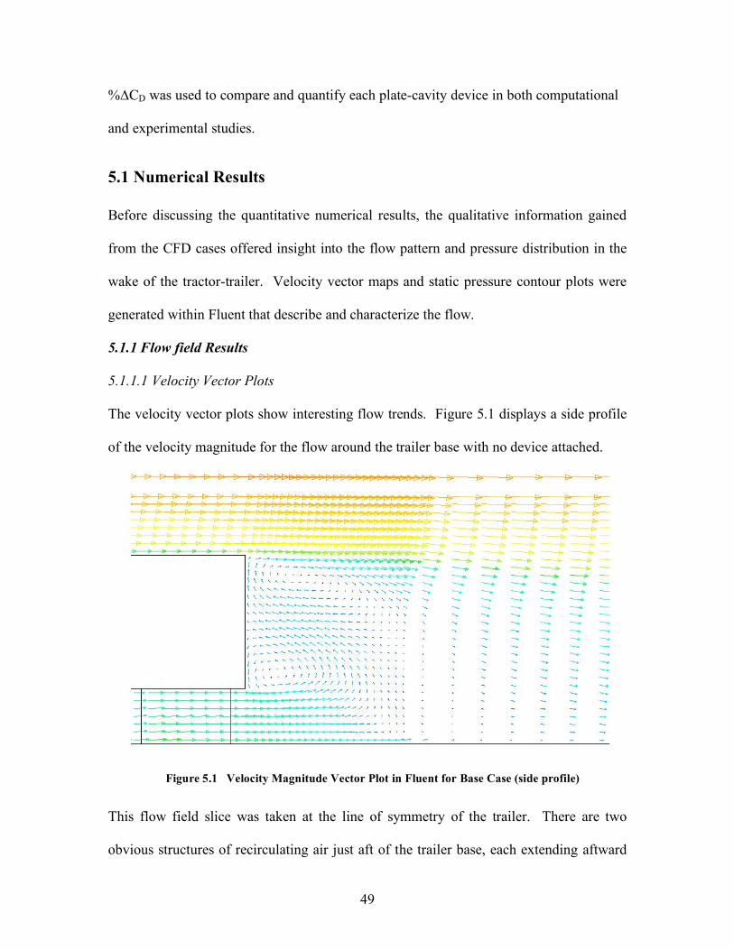
The velocity vector plots show interesting flow trends. Figure 5.1 displays a side profile
of the velocity magnitude for the flow around the trailer base with no device attached.
This flow field slice was taken at the line of symmetry of the trailer. There are two
obvious structures of recirculating air just aft of the trailer base, each extending aftward
Figure 5.1 Velocity Magnitude Vector Plot in Fluent for Base Case (side profile)

50
approximately two-thirds of the trailer base height. There is a streamline at the top of the
trailer. The vortex structure centralized towards the bottom of the trailer base seems to be
the primary structure, while the other centeralized towards the top seems to be secondary
former. It develops slightly aft of the former structure. The flow field may be compared
to a sketch done by Mason and Beebe [13], shown in Figure 4.4, that illustrates the base
region flow of a tractor-trailer. That sketch shows a similar primary recirculation
structure towards the bottom of the trailer as seen in the CFD flow field plot, however, no
indication of a secondary structure is noted.
The addition of a plate-cavity device to the trailer base, shown in Figure 5.2, alters these
structures observed through CFD. The primary structure seems to be larger than previous
inside the cavity in the device case flow field. The flow seems to stagnate more inside
the cavity. The secondary structure still is there, however its presence is lessened due to
the addition of the device.
Figure 5.2 Velocity Magnitude Vector Plot in Fluent for Device Case (side profile)

51
A similar flow field behavior is observed in the top view of the velocity profile for both
the base and device case, seen in Figure 5.3. This flow field slice was taken
approximately at center of the cavity region, and shows two symmetrical structures on
either side just aft of the trailer base in the base case. The flow field at the right shows
similar behavior aft of the plate, however, there is more stagnation inside the cavity
region.
The flow field plots will be helpful when discussing the results for top plate removal in
the experimental results section.
5.1.1.2 Pressure Contour Plots
Contours of the base pressure field were plotted in Fluent to analyze qualitatively the
pressure change from the plate-cavity device addition to the trailer base. Figure 5.4
shows the relative static pressure distribution (psi) for the base and device case. This
pressure field slice was taken at the base of the trailer, and shows the low base pressure
Figure 5.3 Velocity Magnitude Vector Plot in Fluent for Base and Device Case (top profile)

52
region that occurs for the base case. The device addition, indicated by the white outlined
area, increases the pressure at the base.
(a.)
(b.)
Figure 5.4 Base Pressure Distribution Plot in Fluent for Base and Device Case (back profile)
(a.) Base Case (b.) Device Case
53
The numerical pressure distribution results indicate that the addition of a plate-cavity
device builds up the pressure within the cavity, and thus decreases drag on the tractor-
trailer.
5.1.2 Numerical Calculations
5.1.2.1 Pressure Drag Calculations
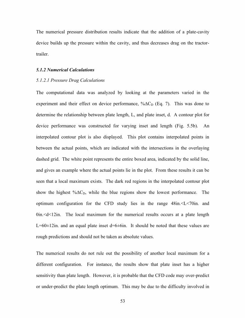
The computational data was analyzed by looking at the parameters varied in the
experiment and their effect on device performance, %!CD (Eq. 7). This was done to
determine the relationship between plate length, L, and plate inset, d. A contour plot for
device performance was constructed for varying inset and length (Fig. 5.5b). An
interpolated contour plot is also displayed. This plot contains interpolated points in
between the actual points, which are indicated with the intersections in the overlaying
dashed grid. The white point represents the entire boxed area, indicated by the solid line,
and gives an example where the actual points lie in the plot. From these results it can be
seen that a local maximum exists. The dark red regions in the interpolated contour plot
show the highest %!CD, while the blue regions show the lowest performance. The
optimum configuration for the CFD study lies in the range 48in.<L<70in. and
0in.<d<12in. The local maximum for the numerical results occurs at a plate length
L=60±12in. and an equal plate inset d=6±6in. It should be noted that these values are
rough predictions and should not be taken as absolute values.
The numerical results do not rule out the possibility of another local maximum for a
different configuration. For instance, the results show that plate inset has a higher
sensitivity than plate length. However, it is probable that the CFD code may over-predict
or under-predict the plate length optimum. This may be due to the difficulty involved in

54
estimating the size of the re-circulating region aft of the trailer. The CFD results were
used in a primarily qualitative manner, due to the coarse grid resolution, and can only
provide information to direct the experimental wind tunnel study. Recall that the purpose
for the numerical study was to approximate an optimum range for both the plate length
and inset.
Figure 5.5 (a.) Schematic of Plate-Cavity Dimensions
(b.) Numerical %!CD Contour and Interpolated Contour L vs. d Plots (EI)
L
d
d (a.)
(b.)
%!CD

55
5.1.2.2 Momentum Drag Calculations
The momentum drag calculation method (refer to sect. 2.2.2) was applied to only a few
selected cases, since the process was time-consuming. Two of the cases chosen were the
base case and the device that yielded the highest %!CD in the CFD study. This device
has a plate length L=60in. and an equal plate inset of d=6in. (full-scale). In comparison
to the %!CD calculated with the pressure drag data, the momentum calculations showed a
much higher prediction for %!CD. The increase is quite large, a jump from 4.18% with
the pressure calculations to 13.62% with the momentum calculations.
The momentum method is a more accurate method for drag calculation since it conserves
momentum from the inlet of the simulated tunnel to the outlet. It also includes drag
contributions from skin friction acting on the tractor-trailer. Thus this method is more
suitable to predict the drag reduction of a specific device. The results from the
momentum calculations are summarized in Table 5.1.
5.1.2.3 Slip Condition Implementation
The CFD cases run used a non-slip condition at all walls. Implementing a slip condition
at the tunnel walls is more representative since it more closely approximates an
unbounded free stream flow. A slip condition at a wall allows free motion along the
plane of the wall, with little inhibition due to possible boundary layer effects. With non-
slip conditions a boundary layer is formed in the simulated experiments that otherwise
Table 5.1 Summary of Numerical Results
Calculation Method Wall Condition Other %!CD
Pressure (sect. 5.1.1) Non-Slip X 4.18
Momentum (sect. 5.1.2) Non-Slip X 13.62
Momentum (sect. 5.1.3) Slip X 17.03
Momentum (sect. 5.1.4) Slip Matched Wind Tunnel Re# 17.35

56
would not exist in real life. If the results from the non-slip cases are similar to those with
slip tunnel wall conditions, it may be said that its effect is negligent at least in these
studies.
The momentum calculation method discussed in the previous section was used to
compare the results for slip and non-slip condition cases since it is assumed to be more
accurate than the pressure calculation method. With the implementation of the slip
condition, the results were noticeably different than with the non-slip condition. For the
geometry with maximum %!CD in the pressure calculations section, the performance
increased from a %!CD of 13.62% to 17.03%. This indicates the significant effect of
implementing the non-slip condition for this particular model.
The implementation of the slip condition may more closely approximate the real-life
situation. However, one point that could be made in favor of the non-slip condition is
that it more closely resembles the conditions in the wind tunnel tests. Since one of the
focuses for this study is to compare the CFD results to the experimental results, the non-
slip condition may be the condition of choice. These results are also summarized in
Table 5.1.
5.1.2.4 Matched Reynolds Number
A comparison similar to the slip/non-slip comparison was performed to see if the results
varied greatly upon matching the CFD model Reynolds number to that in the wind tunnel
studies. As in the slip condition case, the momentum calculation method was used to
quantify the effect of matched Reynolds number. When including this condition along
with the slip wall condition, the %!CD changed slightly from 17.03% to 17.35%. This

57
indicates a small dependence for %!CD on Reynolds number for this model. This
condition’s effect is quite small relative to the slip/non-slip wall condition effect, and is
considered negligible. Results from the matched Reynolds number case are listed in
Table 5.1.
5.1.2.5 Computational Assumptions and Error
There are many assumptions in the numerical study. For example, in the computer
simulation, the model has been fixed to the stationary ground, whereas in real life the
truck would be moving. In this study, the flow forms a boundary later on the tunnel
walls, whereas in real life there exists no boundary layer since the truck moves and the
upstream air is initially stagnant. The model has been approximated with rectangular
shapes, as opposed to the curves that would represent an actual tractor-trailer
combination, especially on the cab. Also, the model neglects small details that influence
the flow around a tractor-trailer, such as the complex underbody of the trailer and
additional exterior fixtures to the trailer. More grid points are necessary to more
accurately quantify the flow around the tractor-trailer model.
5.2 Wind Tunnel Results
There were four different model types tested in the parametric wind tunnel experiment.
They will be referred to as the equal inset case (EI); equal inset, no bottom plate inset
case (EI-0B); equal inset, no top plate case (EI-NT); and equal inset, no bottom plate
inset, no top plate case (EI-0B-NT). Recall that the resolution for the plate insets tested
experimentally was much smaller than that for the numerical study. All data was plotted
in a similar manner as the CFD results. The %!CD data (% drag reduction) was input

58
into the MATLAB code, seen in Appendix A, to generate contour plots and interpolated
contour plots of the %!CD data. Both vertical and horizontal axis limits were
standardized to the limits displayed in the CFD plots. This was done to better compare
the sets of data, including the CFD results. It should be noted that more geometries were
studied in the wind tunnel experiment than in the numerical study. First the equal plate
inset (EI) case will be examined for the zero degree yaw tests.
5.2.1 Zero Degree Yaw Test Results
5.2.1.1 Equal Inset
This data proved to be very essential since it serves as somewhat of a control experiment
for the other three model types tested. Figure 5.2 illustrates the results for the EI case
displayed in contour plots, which show a local maximum for %!CD. The first plot shows
%!CD contours, with varying plate length L and plate inset d. The adjacent plot shows a
diferent visual picture of the local optimum for both L and d, through the use of
interpolated contours. The geometries tested are indicated by the intersections in the
overlaying dashed grid (Fig. 5.6). Recall that the resolution of the plate inset, d, for the
experimental models was 1.91in., as opposed to the resolution in the numerical study of
6in.

59
The plots indicate a strong sensitivity of %!CD to plate inset as compared to plate length.
The data indicates an optimum geometric configuration within the range 45in.<L<55in.
and 3in.<d<7in. full-scale. Within these constraints %!CD ranges from 8.0-8.84%. The
maximum %!CD was achieved with a geometric configuration of L=48in. and d=5.72in.,
yielding an 8.84±2.37 reduction in drag. The associated error for the %!CD quantities
will be later discussed.
5.2.1.2 Effect of Zero Bottom Plate Inset
The equal inset, zero bottom plate inset case data (EI-0B) looks very similar to that of the
EI case, in that the geometries that performed best are in very similar optimum geometric
ranges. However, as seen in the interpolated contour in Fig.5.7, a local maximum is not
obviously present. For instance, there is no clear indication of an optimum range for
Figure 5.6 Experimental %!CD Contour and Interpolated Contour L vs. d Plots (EI)
%!CD
L d
d

60
plate length L. For maximum performance, the plate length should be L>45in., however,
no information can be derived from the data for an upper limit for L. The optimum range
for plate inset lies within 3in.<d<8in., with a %!CD range from 8.5-9.03%. The
maximum %!CD for the EI-0B case was achieved with a geometric configuration of
L=48in. and d=5.72in., yielding an 9.03±2.26 reduction in drag. Almost identical results
were achieved for the case with L=60in. and d=5.72in.
When comparing the EI case to the EI-0B case, improved results are achieved by
positioning the bottom plate with zero inset. Assuming that the local maximum observed
in the EI case is absolute, it may be said that the placement of the bottom plate with d=0
is beneficial to reducing the drag. With this configuration a streamline is forced at the
bottom-most part of the trailer. Recall that the purpose of the plate inset is to allow
Figure 5.7 Experimental %!CD Contour and Interpolated Contour L vs. d Plots (EI-0B)
%!CD
L d
d
61
separation at the trailing edges of the trailer and to force vortex formation. This strategy
for drag reduction works best for the top and sides of the trailer. The bottom plate works
best when forcing a streamline rather than forcing vortex formation.
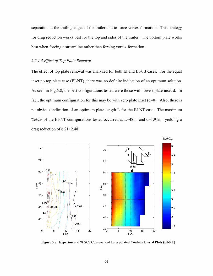
5.2.1.3 Effect of Top Plate Removal
The effect of top plate removal was analyzed for both EI and EI-0B cases. For the equal
inset no top plate case (EI-NT), there was no definite indication of an optimum solution.
As seen in Fig.5.8, the best configurations tested were those with lowest plate inset d. In
fact, the optimum configuration for this may be with zero plate inset (d=0). Also, there is
no obvious indication of an optimum plate length L for the EI-NT case. The maximum
%!CD of the EI-NT configurations tested occurred at L=48in. and d=1.91in., yielding a
drag reduction of 6.21±2.48.
Figure 5.8 Experimental %!CD Contour and Interpolated Contour L vs. d Plots (EI-NT)
%!CD
L d
d

62
More conclusive information could be drawn from the results obtained for the EI-0B-NT
case. The contour plots indicate a more defined range for optimum plate inset (Fig.5.9).
As in the EI-0B case, there exists a lower limit of L=45in., but no clear higher limit for
plate length. The model type EI-0B-NT operates best when plate inset is in the range
2in.<d<5in, yielding a %!CD range from 5.8-6.3%. The maximum %!CD occurs with
L=60in. and d=3.81in., %!CD=6.34±2.44. Note that this is closely followed by the
configuration having L=48in. and d=3.81in., %!CD=6.27±2.37. The results for
maximum %!CD for all model types are summarized in Table 5.2.
Figure 5.9 Experimental %!CD Contour and Interpolated Contour L vs. d Plots (EI-0B-NT)
Table 5.2 Summary of Experimental Results
%!CD
L d
d
Geometric Variations Optimum Range Local Maximum
Case Equal Inset Bottom Plate d=0 No Top Plate L (in.) d (in.) L (in.) d (in.) %!CD
EI X 45<L<55 3<d<7 48 5.72 8.84±2.37
EI-0B X X L>45 3<d<8 48 5.72 9.03±2.26
EI-NT X X N/A 0<d<4 48 1.91 6.21±2.48
EI-0B-NT X X X L>45 2<d<5 60 3.81 6.34±2.44

63
The effect of removing the top plate decreases the performance for all four-plate
configurations tested. This occurs for both the EI-NT and EI-0B-NT cases. For the EI-
NT case, the optimum geometry yields a %!CD of about 70% of the %!CD achieved with
the optimum geometry in the EI case. For the EI-0B-NT case, the optimum geometry
also yields a %!CD of about 70% of the %!CD achieved with the optimum geometry in
the EI-0B case.
5.2.1.4 Shift in Optimums
When comparing the EI case to the EI-NT case, a shift in optimums is observed. Recall
that the EI case results indicated an optimum range for plate inset of 3in.<d<7in (Table
5.2). The optimum range for the plate inset in the EI-NT case occurs at a lower range of
0in.<d<4in. Thus there seems to be a decrease in optimum plate inset when removing the
top plate from a configuration.
A similar trend is observed when comparing the EI-0B case results to that of the EI-0B-
NT case results, in that a shift in optimums has occurred. The EI-0B case results indicate
a local maximum within the range 3in.<d<8in. However, the EI-0B-NT case results
indicated maximum performance within the range 2in.<d<5in. This suggests that a shift
in optimum d has also occurred from the EI-0B case to the EI-0B-NT case. It is unclear
if top plate removal causes the optimum plate length to increase or decrease.
Two suggestions are presented to explain the shift in optimum plate inset due to top plate
removal. The data shows that the removal of the top plate of a configuration (EI-NT, EI-
0B-NT) in general causes the optimum plate inset range to decrease from that for the case
with the top plate (EI, EI-0B). There exists a large low-pressure region of air at the base

64
of the trailer with no device attached. Recall that one of the functions of the plate-cavity
device is to trap higher pressure air in the cavity, due to the separation off the plate
trailing edges. The removal of the top plate allows for this higher pressure air to escape,
thus lessening the pressure inside the cavity.
One suggestion is that in order to maintain a high pressure inside the cavity, it is
necessary to encourage separation off the plate trailing edges. The plates, when inset
towards the center of the trailer base, are masked from the oncoming flow, and vortex
shedding off the plate trailing edges may be lessened. Upon speculation, a way to
encourage separation would be to move the remaining plates closer to the perimeter of
the trailer. This may allow for increased vortex shedding off the plates and into the
cavity region. Another suggestion is that moving the plates towards the perimeter of the
trailer increases the size of the cavity and therefore traps a higher volume of air. There is
no experimental base pressure data to support either of these suggestions as they are
speculative. The comparisons for all four model types may be seen in Appendix D,
which contains all four interpolated contour plots on the same page.
5.2.2 Yaw Test Results
5.2.2.1 Plate Cavity Designs
Measurements were acquired on plate-cavity devices for yaw tests from –3° to +9°, with
an increment of 3°. The plate-cavity devices tested were comprised of select model
configurations from the zero degree tests. The models that yielded the highest %!CD
were chosen and tested. These configurations are summarized in Table 5.3.

65
The yaw results give a lot of information about the general behavior of each model at low
angles, for example over ±3°. The results for %!CD at specific yaw angles can be seen in
Fig.5.10. The legend in Fig.5.10 uses the device nomenclature to describe each device
tested. Figure 5.11 explains the device nomenclature.
Table 5.3 Plate-Cavity Models Tested in Yaw Study (optimum highlighted)
Figure 5.10 %!CD vs. Yaw Angle for Various Plate-Cavity Devices
4_3.81_0b_notop Full-Scale Plate
Length, L (ft.)
Full-Scale Plate
Inset, d (in.)
Bottom Plate
Inset d=0
No Top Plate
Figure 5.11 Legend Explanation for Yaw Angle Plot
Plate Parameters (Full-Scale) Characteristics
L (in.) d (in.) Equal Inset Bottom Plate d=0 No Top Plate
48 5.72 X X
48 3.81 X X
48 3.81 X X X
36 3.81 X X
-2
-1
0
1
2
3
4
5
6
7
8
9
-3 0 3 6 9
Yaw Angle (Degrees)
%!
CD
4_3.81_0b_notop
4_5.72_0b
4_3.81_0b
3_3.81_0b

66
For all configurations tested, and at low angles, the behavior of the drag with yaw angle
is concave down. In other words, %!CD decreases with increasing yaw angle. The
device with maximum %!CD from the zero degree tests, with L=4ft., d=5.72in., and d=0
for the bottom plate (4_5.72_0b), performed well at low yaw angles (Fig.5.10). Note that
for all configurations tested with 4 ft. plate length, the concave down behavior continues
for all yaw angles. The behavior changes at higher yaw angles for the model with L=3ft.,
d=3.81in., and d=0 for the bottom plate (3_3.81_0b). The drag data starts to level off at
+6º (Fig. 5.10). This may be attributed to the effect of less area exposed to the flow with
a shorter plate length L. The drag will decrease with less exposed area since the drag on
the tractor-trailer is a function of area. The difference in %!CD for all 4 ft. models tested
at a given yaw angle is consistent over the entire range of yaw angles.
The removal of the top plate, as in the case with L=4ft., d=3.81in., and d=0 for the
bottom plate (4_3.81_0b_notop), has an adverse effect on drag reduction for the range of
yaw angles tested, in comparison to all the 4-plate models tested (Fig.5.10). Also, the
difference in %!CD for the no top plate model tested for a particular yaw angle is
consistent over the entire range of yaw angles, when compared to 4-plate model with the
same geometry (4_3.81_0b). The conclusion is that top plate removal is detrimental to
performance over the entire range of yaw angles tested.
5.2.2.2 Angled Plate Designs
Yaw tests were also conducted on variations of the MAKA patented angled plate design.
As previously mentioned, the MAKA design utilizes angled plates (as opposed to plates
perpendicular to the trailer face) to direct the flow inward at the aft of the trailer. This

67
design does not include a plate inset for any of the three plates that are placed at a 15°
angle with respect to the trailer top and sides. As with the plate-cavity device yaw testing
data, there is more curious and unexpected behavior above +3° yaw for the MAKA
variations. Figure 5.12 shows the results for %!CD at specific yaw angles.
For the MAKA design at low yaw angles, the behavior is concave up. In other words, the
data suggests that %!CD increases with increasing yaw angle over the range ±3°. The
behavior is similar for the inverted MAKA case as well. Actually, the results indicate a
better performance for the inverted case over ±3°. This may be due to the necessity of a
bottom plate, as established in the zero degree tests. The addition a straight bottom plate
to the original MAKA design was analyzed as well. Over ±3°, the addition of the bottom
plate in the 4-plate MAKA design improves the performance of the MAKA substantially.
Figure 5.12 %!CD vs. Yaw Angle for MAKA Patent Variations and Plate Cavity Device
-3
-2
-1
0
1
2
3
4
5
6
7
8
-3 0 3 6 9
Yaw Angle (Degrees)
%!
CD
MAKA
Inverted MAKA
4 Plate MAKA

68
For example, at 0°, the %!CD increased from 3.19% for the MAKA case to 6.05% for the
4-plate case.
At higher yaw degrees, the results are more unexpected and difficult to explain. For
example, for both the MAKA and 4-plate MAKA, the %!CD data decreases at +6°. For
the MAKA case, this occurs after concave up behavior in the range ±3°. One explanation
for this is that the angled plates in the MAKA design offer a compromise over the range
of yaw angles. In other words, at zero degrees, the performance is not optimized. It is
possible that some yaw angle there exists an optimum %!CD. Since the data suggests
that %!CD decreases from +3° to +6°, there is some evidence of this. However, it is
apparent that more data points are necessary in order to validate this. The behavior at +9°
is also very inexplicable. For example, the behavior for both the MAKA and 4-plate
MAKA design continue to have similar shape, in that %!CD again rises at +9°. The 4-
plate design achieved a higher %!CD at this yaw angle.
The behavior of the inverted MAKA design is different from that of the original design.
At +6°, the inverted case continues its convex behavior (as experienced over ±3°). This
differs from both the MAKA and 4-plate MAKA cases. The common element in the
MAKA and 4-plate cases that differs from the inverted case is the presence of a top plate.
It is possible that a negative effect from the top plate is occurring at +6°. This is
confusing since at +9° the trend is reversed. In other words, at +9°, the 4-plate MAKA
outperforms both the original and the inverted MAKA designs. It should be noted that
the data points that occur at both +6° and +9° are within the experimental error of the
other devices. The error on those data points shows that no conclusions may be made

69
about those data points with respect to the other devices tested. The error will be
discussed thoroughly in the following section.
Intuitively, one might hypothesize that the presence of a flat bottom plate would improve
the %!CD over the original design over all angles of yaw. The results from the zero
degree tests indicate the necessity for the bottom plate at the very bottom of the trailer.
However, as indicated in the yaw tests, one data point (+6°) suggests that the 4-plate
MAKA may not perform as well as the inverted device. The general conclusion in the
yaw tests is that more data points are necessary at many more yaw angles to fully
substantiate any claims made for yaw trends of the MAKA design, or any of its
variations.
5.2.3 Wind Tunnel Error Estimates
The Kline-McClintock error estimation method was used to bound the wind tunnel
measurements [24]. Both the instrument error and quantization error were included for
all instruments used. Before discussing the error on the performance, %!CD, for the
devices, it is necessary to discuss the error on the factors that propagate into the %!CD
error. Figure 5.13 shows a plot of the error bounds on CD for varying plate insets and
plate lengths. This data is from the zero yaw degree tests. The error bars on the data for
devices with plate length L=3ft. show that the data is independent of the data obtained for
CD for devices with L=4,5ft. The CD data for L=4ft and L=5ft., however, is similar and
contained within the respective error bars.

70
The error on CD for each particular device then propagates with the "CD error. Assuming
that the error on the base case CD and device CD are equal, the error on the difference,
"CD, is roughly (#2)*(uncertainty in CD). Figure 5.14 shows a plot of the error bounds
on "CD for varying plate insets and plate lengths. The error has been magnified since a
difference is being taken. The difference ("CD) is small compared to the original
counterparts (base CD and device CD). The error bounds on the L=5ft. data encompass
the data from the other plate lengths, indicating that the effect of looking at error on "CD
magnifies the actual error on CD.
Figure 5.13 Error Bounds on CD vs. Full Scale Inset Plot for Various Plate-Cavity Devices
(Zero Yaw Degree)
0.65
0.67
0.69
0.71
0.73
0.75
0.77
0.79
0.81
0.83
0.85
0 2 4 6 8 10 12 14 16 18 20 22
Full Scale Inset (in.)
CD
5 feet
4 feet
3 feet

71
The error propagation then continues into the %!CD error calculation. Figure 5.15 shows
a plot of the error bounds on %!CD for varying plate insets and plate lengths. The error
bars shown indicate that for every data point, the error is large. The error bounds on the
L=5ft. data encompass the data from the other plate lengths. The error on %!CD is a
magnification of the actual error on CD, in a similar manner as is the "CD error. The
prime contributor to the error in the measurements is the differential pressure transducer
that measures the pressure drop in the contraction of the wind tunnel inlet. The error
increases slightly under conditions of yaw. A sample error calculation is included in
Appendix E.
Figure 5.15 suggests that the %!CD data may not be differentiable due to the large error
associated with each of the values. However, it should be noted that for every case where
the top plate was removed, the performance decreased. For every case where the bottom
0
0.01
0.02
0.03
0.04
0.05
0.06
0.07
0.08
0.09
0.1
0 2 4 6 8 10 12 14 16 18 20 22
Full Scale Inset (in.)
!C
D
5 feet
4 feet
3 feet
Figure 5.14 Error Bounds on !CD vs. Full Scale Inset Plot for Various Plate-Cavity Devices
(Zero Yaw Degree)

72
plate was placed to the bottom of the trailer base, the performance increased. These data
consistencies contribute a higher level of confidence in the data than the error
calculations display.
In addition to the instrumentation and quantization error, it is important to consider other
possible sources of error in this experiment. For example, one point of discussion lies in
the repeatability of the force balance setup. It is important for the balance to give a
similar output each time when loaded, when testing a particular device on the trailer. In
order to counter this concern, the data was taken several times for each case. The force
balance was loaded several times with data taken each time. These data points were then
averaged. Another concern lies in the shift in base reading for the truck without a device
attached. This may be due to a drift in calibration due to changes of conditions in the
Figure 5.15 Error Bounds on %!CD vs. Full Scale Inset Plot for Various Plate-Cavity Devices
(Zero Yaw Degree)
0
2
4
6
8
10
12
0 2 4 6 8 10 12 14 16 18 20 22
Full Scale Inset (in.)
%!
CD
5 feet
4 feet
3 feet
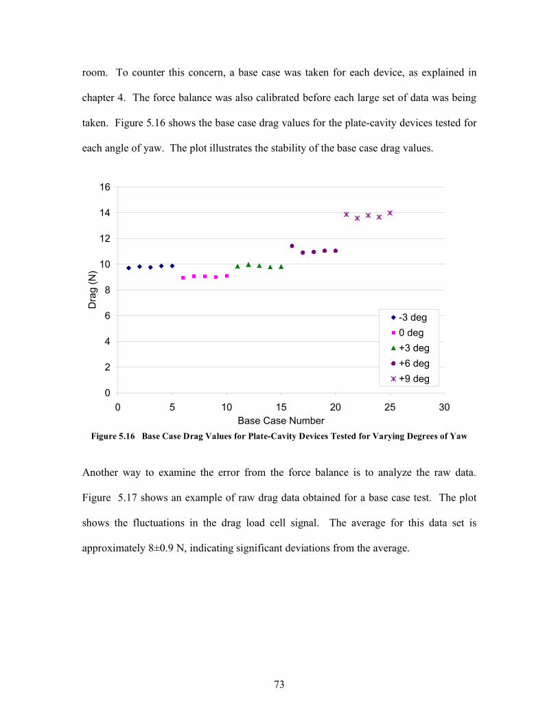
73
room. To counter this concern, a base case was taken for each device, as explained in
chapter 4. The force balance was also calibrated before each large set of data was being
taken. Figure 5.16 shows the base case drag values for the plate-cavity devices tested for
each angle of yaw. The plot illustrates the stability of the base case drag values.
Another way to examine the error from the force balance is to analyze the raw data.
Figure 5.17 shows an example of raw drag data obtained for a base case test. The plot
shows the fluctuations in the drag load cell signal. The average for this data set is
approximately 8±0.9 N, indicating significant deviations from the average.
Figure 5.16 Base Case Drag Values for Plate-Cavity Devices Tested for Varying Degrees of Yaw
0
2
4
6
8
10
12
14
16
0 5 10 15 20 25 30
Base Case Number
Dra
g (
N)
-3 deg
0 deg
+3 deg
+6 deg
+9 deg

74
After a data set is recorded, another data set is taken and averaged. Figure 5.18 shows the
average of numerous data sets for a two typical base case data sets. These values are
close and more consistent with each other than is the raw drag data. The first data set
(Base1-Figure 5.18) shows that the averaged data is roughly 7.99±0.02 N. The raw un-
averaged data obtained is within a much larger range. The second data set (Base2-Figure
5.18) shows that the averaged data is roughly 7.95±0.02 N, displaying a similar
consistent trend with the averaged values.
0
1
2
3
4
5
6
7
8
9
10
0 20 40 60 80 100 120
Data Point
Dra
g (
N)
Figure 5.17 Raw Drag Data for Base Case Example

75
5.3 Results Comparison
5.3.1 Computational/Experimental Results
The computational and experimental results may be compared for the equal inset case
(EI). The contour plots of the results for each, are conveniently displayed next to each
other for easier comparison in Fig.5.17. There was increased resolution for the plate
insets tested in the experimental plot, indicated by the dashed overlaying grid. The CFD
results presented here are the pressure calculations previously discussed. There is also
one point in the CFD results plot that displays the configuration for which the momentum
calculation was performed (refer to section 5.1.2.2). This particular point, indicated by a
white dot, represents a %!CD of 13.62% (Fig. 5.17). The major difference in the
experimental results and numerical results (pressure calculations) is the magnitude
Figure 5.18 Averaged Raw Drag Data for Base Case Data Sets
7.9
7.91
7.92
7.93
7.94
7.95
7.96
7.97
7.98
7.99
8
8.01
8.02
0 1 2 3 4 5 6 7 8 9 10 11
Data Set
Dra
g A
ve
rag
e (
N)
Base2
Base1

76
(a.)
(b.)
Figure 5.19 Numerical and Experimental Comparison –Interpolated Contour L vs. d Plots (EI)
(a.) Numerical Results (b.) Experimental Results
%!CD
L d
d
%!CD

77
of %!CD. For example, the optimum configuration in the CFD experiments yielded a
drag reduction of approximately 4.18%, while the maximum %!CD for the wind tunnel
experiments was approximately 8.84% (EI case). The wind tunnel measurements are
more than twice as great as the CFD data. This is most likely due to the method of
calculation, as well as the amount of error present in such a crude model. As discussed
early, the momentum calculation is more accurate than the pressure drag calculation
method. It suggests a greater reduction in drag for the plate-cavity devices than the wind
tunnel measurements show. This is contrary to the pressure drag calculation method,
which underestimates the measurements observed in the wind tunnel.
Another difference in the comparison of the CFD and wind tunnel results, is the plate
length L at which a local maximum is achieved. The CFD suggests a higher value for
plate length. It is possible that the CFD may have over-predicted the wake size on the
bluff body. A longer plate length would be necessary to keep attachment on the trailer
extension. The suggested ranges for plate inset d are similar when comparing the
computational and experimental results. These results are summarized in Table 5.4.
5.3.2 Comparison to Previous Work
The results from the computational and experimental data can be compared to that of
Bilanin [11] and Lanser, et al [15]. In order to compare the results to these two published
Table 5.4 Computational and Experimental Results Comparison Summary (Zero Yaw Degree)
%CD
Geometric Optimum Ranges Geometric Maximums
Plate Insets (in.) Plate Insets (in.)
Case Study Plate Length (in.) Top Sides Plate Length (in.) Top Sides
Computational 48<L<70 0<d<12 0<d<12 60 6 6
Experimental (EI) 45<L<55 3<d<7 3<d<7 48 5.72 5.72

78
studies, it is necessary to define the parameters used to classify the optimum geometry.
The two published results will be compared separately to the present results. Both
published optimum results have been presented here as non-dimensionalized quantities.
The plate insets, G and D, and the plate length, L, have been non-dimensionalized by the
trailer width, W. These are summarized below (refer to Fig.5.18).
G/W = top plate inset to trailer width ratio
D/W = side plate inset to trailer width ratio
L/W = plate length to trailer width ratio
As can be seen in Table 5.5, the present results for optimum geometry differ from that of
Bilanin. In terms of plate placement, both the Bilanin and Lanser, et al published
geometries compare most closely to the present experimental case with zero bottom plate
inset, since they all have the same bottom plate position (row 3 –Table 5.5). The Bilanin
published optimum geometries (row 4 – Table 5.5) are different than those seen in the
current computational and experimental studies. The G/W and D/W (refer to Fig.5.18)
G
H
D
L
W
Figure 5.20 Dimensions for Plate-Cavity Device (trailer base view)

79
inset ratios reported by Bilanin are twice as great as the current experimental inset ratios,
indicating higher optimum plate insets for the Bilanin design. In the patent, Bilanin also
specifies a range for optimum inset ratio of 0.1<G/W=D/W<0.2. The current
experimental values lie outside this range at G/W=D/W=0.06.
The plate length ratio reported by Bilanin of L/W=0.44 is less than that of the present
optimum at L/W=0.504. However, it should be noted that Bilanin also specified that the
full-scale range for optimum plate length should be in between 40in.<L<56in. An
average trailer has a common width of about W=100in. Correlating the current
experimental results with this trailer width, the plate length would be about 50in., which
lies in the plate length range specified by Bilanin.
The experimental results are then compared to those of Lanser, et al (row 5 – Table 5.5).
In terms of plate inset ratios, very similar results occur. The experimental cases compare
exactly at G/W=D/W=0.06. The plate length ratio differs, from L/W=0.504 for the
experimental case with zero bottom plate inset, to L/W=0.36 for Lanser, et al. However,
as discussed earlier, the plate inset has a much stronger influence on drag reduction than
does the plate length. Also, the number of different plate lengths tested experimentally
Table 5.5 Optimum Geometry Summary for Current and Published Results
Geometric Optimums
(non-dimensionalized by trailer width)
Plate Length Plate Insets
Results L/W G/W=D/W
Computational - present 0.625 0.063
Experimental (equal inset) - present 0.504 0.060
Experimental (bottom plate inset=0) - present 0.504 0.060
Bilanin [11] 1987 0.44 0.13
Lanser, Ross, Kaufman [13] 1991 0.36 0.06

80
are few in comparison to the number of different plate insets tested. The current plate
length optimum ratio corresponds to a full-scale plate length of 4ft. The other two plate
lengths tested experimentally of 3ft. and 5ft. correspond to L/W=0.375 and L/W=0.625,
respectively. The optimum plate length ratio may lie anywhere in this range. As the
experimental results show, the optimum plate inset is more crucial to reducing drag. The
agreement between the present and published results for plate inset is encouraging.

81
Chapter 6: Conclusions and Recommendations
6.1 Conclusions
A parametric wind tunnel experiment was performed in Clarkson University’s subsonic
wind tunnel to measure the drag with different attachment geometries at the base of a
scale model tractor-trailer. Experiments were complemented with a numerical study
using Fluent, which assisted in directing the wind tunnel experiment. Both numerical and
wind tunnel studies involved varying geometric parameters of plate-cavity designs added
to the base of the tractor-trailer. The studies helped to find an optimum range for plate
length, L, and plate inset, d. The computational results support the data observed in the
wind tunnel.
Four plate-cavity variations were tested experimentally, each consisting of their own
parametric study. The models all consisted of plates mounted perpendicular to the trailer
base, and were all tested at zero degree yaw. All results indicate a higher sensitivity for
plate inset on drag reduction than for plate length.
The results of having the bottom plate inset, d, set to the bottom of the trailer base
supported the claim of previous research that suggests that this particular bottom plate
placement is essential to reducing the base drag. The experimental data supports this

82
claim. The effect of top plate removal was examined experimentally and found to be
detrimental to the drag reduction of the tractor-trailer. This was evident in both cases:
equal plate inset for all four plates (EI), and bottom plate inset set at zero (EI-0B). The
removal of the top plate may be influential in realizing the practical role of such a device
on a full-scale level.
The numerical and experimental results compare well in terms of plate inset, d. The
results indicated a range for optimum inset of 0<d<12in. (numerical), and 3<d<7in.
(experimental). The optimum plate length suggested computationally is longer than that
observed in the wind tunnel. However, the numerical study was a very rough model and
was considered as a tool for directing the experiments.
Experimental results were compared to the published results. The most important finding
was that the optimum experimental plate inset, d, was found to agree very closely to that
of Lanser, et al [13], the most recent parametric study performed prior to the present.
The experimental models tested that compare closest with those tested by Lanser, et al
are those with the bottom plate inset set at zero. As previously stated, the plate inset is a
more important factor than is plate length towards reducing drag. The current results
show that alterations may be made to the optimum plate length and not affect the drag
reduction significantly, whereas a deviation from the optimum plate inset will
significantly affect the performance. This fact that the experimental and published
optimum plate insets agree is very encouraging.
A limited set of yaw tests were also conducted to examine the effects of yaw angle on
performance for those plate-cavity devices that performed best in the zero degree tests.
83
Also tested were angled plate devices, where the plates were no longer mounted
perpendicular to the trailer base, as before, but at an angle inward of the trailer perimeter.
Variations to the MAKA Innovation angled plate patented design were constructed and
tested.
The device performance decreased as yaw angle increases for the plate-cavity devices
mounted perpendicular to the trailer base. This was consistent for all devices tested
without angled plates. The device that achieved the highest drag reduction on the trailer
was consistently more efficient at reducing drag compared to all of the other plate-cavity
devices tested at small angles of yaw. At higher angles of yaw, the devices with shorter
plate length reduce drag more effectively, possibly due to less exposed frontal area. The
longer plate length devices may increase the frontal area of the trailer at high yaw angles.
Each of the angled plate design variations displayed a concave up behavior at low yaw
angles, contrary to the concave down behavior of the perpendicular plate-cavity devices
previously mentioned. There is curious and unexpected drag reduction behavior at higher
yaw angles, as the concave up behavior does not always persist for all devices tested for
all angles of yaw. At small angles of yaw, the four-plate modified MAKA design
achieved the highest drag reduction, indicating the importance for the bottom plate. One
conclusion that may be made for all devices, not just the angled plates, is that the
existence of the bottom plate is crucial to the performance of the plate devices tested.
6.2 Recommendations for Future Study
Several changes to both the numerical and experimental studies can be made to further
analyze the effects of non-ventilated plate-cavity devices at the base of tractor-trailers.

84
Both studies have room for improvement as well as room for continued study on
variations to the plate-cavity geometry.
The numerical parametric study would benefit from the addition of the slip wall
condition, in placement of the non-slip placed at the walls of the simulated tunnel walls in
the present study. This would closer approximate the conditions in real life. It would
also be beneficial to use the momentum calculation method to quantify the performance
of each plate device case ran in CFD. The most important thing to change concerning the
current model is increasing the number of grid points. It would be interesting to see if
doubling the grid points greatly changes the results of the trends observed with the coarse
grid. The current model has too few points to be able to accurately calculate a separated
flow at the trailer base.
The wind tunnel experiment would benefit from a number of changes to the setup. For
example, the force balance is externally located under the test section. The sting connects
the trailer model to the balance, however, is quite long. The balance could be raised
closer to the bottom of the test section, thus making the sting shorter. This will decrease
the displacement at the end of the sting and reduce the oscillations experienced by the
tractor-trailer model when loaded. Another change that could be made to the experiment
would be to calibrate the load cells with more weights, the majority of the weights being
in the range of the expected loads. This would increase the accuracy of the
measurements.
The experimental error should be given long consideration for further improvement. The
prime contributor to the experimental error, the differential pressure transducer, should be

85
replaced with a more suitable device. The current device has a span of 0-2 in. H2O,
however, the pressure measurements taken in the tunnel have all been in the range
0<!P<1.10 in. H2O. The Modus DT pressure transducer could be replaced with a similar
model with span 0-1.25 in. H2O, which will decrease the experimental error significantly.
If it would not be possible to obtain a transducer with such a span, it would be advisable
to procure one with a higher accuracy.
It would be beneficial to test more devices with several different plate lengths. The
present study only consisted of models with 3, 4, and 5 ft. plate lengths. As a general
rule, the plate length was not as sensitive to the drag reduction of the plate devices as was
plate inset. Additional plate lengths tested will confirm or refute the previous results.
Another suggestion that would benefit the experiment would be to include zero plate
inset cases for all model types. Recall that the lowest plate inset tested in the EI-NT case
achieved the maximum %CD. Perhaps with zero plate inset the greatest drag reduction is
achieved.
The effect of top plate removal could be investigated experimentally more thoroughly
through the use of pressure taps at the trailer base. Mapping the pressure distribution
within the cavity may help to explain the shift in optimum plate inset discussed in Section
5.2.1.4. Theses measurements will also help to quantify the base pressure increase due to
the addition of the plate-cavity device.
Extensive yaw testing is necessary to confirm the results observed in the limited set of
tests. This is more crucial in the angled plate study. Curious and unexpected behavior
occurs at higher yaw angles, and merits further study.

86
Appendices

87
Appendix A:
MATLAB Contour Code
% dragcontour.m
%
% This program takes drag reduction data files with information
% from a parametric study, including plate inset, plate length, and
% %CD then creates a uniform grid based on the given coordinate
% positions and linearly interpolates the desired functional values
% at the new locations.
%
% The data is then plotted in three ways --> contour plots,
% interpolated color plots, and 3-D surface plots.
%
%
% Used with permission
% Code by Dave Schmidt, ME Dept., Clarkson University
clear all
%-----Read data
load drag.dat
data = drag;
minx = 0.0;
maxx = 20.0;
miny = 35.0;
maxy = 72.0;
dx = 2.0;
dy = 1.0;
%-----Assignments
x(:,1) = data(:,1);
y(:,1) = 12.0.*data(:,2);
z(:,1) = data(:,3);
%-----Define a uniform grid
gridx = minx:dx:maxx;
gridy = miny:dy:maxy;
[Xgrid,Ygrid] = meshgrid(gridx,gridy);
%-----Interpolate functional values to grid
Zdata = griddata(x(:,1),y(:,1),z,Xgrid,Ygrid);
%--------------------------- PLOTTING -----------------------------
%-----U instantaneous
h5 = figure;
contour(Xgrid,Ygrid,Zdata,10)

88
clabel(contour(Xgrid,Ygrid,Zdata,20))
xlabel('\it{d (in)}','Fontsize',10,'Fontname','Times-Roman')
ylabel('\it{L (in)}','Fontsize',10,'Fontname','Times-Roman')
axis image
h6 =figure;
pcolor(Xgrid,Ygrid,Zdata),shading interp
xlabel('\it{d (in)}','Fontsize',10,'Fontname','Times-Roman')
ylabel('\it{L (in)}','Fontsize',10,'Fontname','Times-Roman')
axis image
h7 = figure;
surf(Xgrid,Ygrid,Zdata),shading interp
xlabel('\it{d (in)}','Fontsize',10,'Fontname','Times-Roman')
ylabel('\it{L (in)}','Fontsize',10,'Fontname','Times-Roman')
axis image
% print -depsc -tiff -r600 ucontourc
% print -deps ucontour.eps
% print ucontour.ps
% colormap(winter)
% colorbar('horiz')
% axis tight
% axis image
% orient landscape
% print( -djpeg )

89
Appendix B:
Additional Experimental Setup Pictures
Figure B-2 Experimental Bracing Procedure
Figure B-1 Experimental Model Connection to Sting

90
Figure B-3 Steel Backing to Experimental Tractor-Trailer Model
Figure B-4 Experimental MAKA Model Attached to Trailer Base

91
Appendix C:
Wind Tunnel Operation Procedure
I. Summary of System
The Trailer Drag Reduction System at Clarkson University contains many physical
components as well as software components that take the data from the physical
components and display the data graphically. The system is not exclusive to the Trailer
Drag Reduction program, as the whole system or individual components of the system
may be used for a number of other wind tunnel applications.
Physical Components
There are many devices that constitute the drag reduction system, but may be used
separately in other applications as well. These include the two devices in the
force balance constructed at Clarkson University, including the drag and side
force load cells. Other devices include a differential pressure transducer, an
atmospheric pressure transducer, and a temperature transmitter. All devices
interface with the control computer. The computer is equipped with 2 National
Instruments Data Acquisition cards model PCI6024E.
Software Components
All data acquisition is controlled via one LabVIEW Virtual Instrument (VI). This
program acquires data from all five devices and outputs them to files. Each
instrument is sampled at a specifies sample rate and output in array form to file.
The drag calculations were made manually, and then input into a MATLAB code
for plotting purposes.
II. Setup of System
Prior to data acquisition, the components of the system must be properly oriented and
setup.
(a.) Force Balance
There are several key things to remember to check prior to testing in the tunnel
concerning the force balance. One is that all fasteners on the force balance must be
secure, most importantly the connections to the load cells and the linear roller bearing
translators. Secondly, it is imperative that the base board for the balance (the !” sheet
steel base, not the 1” plywood base) is leveled. There are rubber washers underneath the
supports on the steel base that allow the four screws to be adjusted for leveling purposes.
Do not allow unauthorized persons to touch the force balance.

92
(b.) Tunnel Floor Board
The floor board for the tunnel must then be securely placed in the test section of the
tunnel. Make sure to properly orient the direction of the board, as there is a front and
back, as well as a top and bottom.
(c.) Modeled Ground Plane
Before placing the modeled ground plane in test section, steel washers must be placed
over the holes in the tunnel floor board. The modeled ground plane has 8 threaded rods
mounted perpendicular to the base that fit into the holes. These threaded rods must each
have their own bolt to provide a stop for the rods, as well as enable leveling of the ground
plane. Adjust the height of the ground plane so that the tractor-trailer model will be close
the center of the test section. Once leveling is completed, the threaded rods must be
secured from underneath the tunnel floor board with washers and bolts.
(d.) Sting
Slide the sting into the designated hole and attach to the force balance sting receptacle
and secure with the setscrews. Be careful not to jar the balance as damage may be done
to the load cells. Do not allow unauthorized persons to touch the sting, as it is
physically connected to the load cells in the force balance.
(e.) Truck Model
The installation of the truck model in the setup requires two people. Loosen both
setscrews in the trailer sting receptacle, which should be physically connected the the
entire tractor-trailer model. One person must hold the model above the ground plane,
with the sting inside the receptacle, setscrews still loosened. The other person must
determine the height at which the model will not touch the ground plane. The setscrews
are then adjusted to tighten and secure the model. The model height may need to be
raised slightly if the wheels touch the ground plane when the model is loaded. No
unauthorized persons should operate the tunnel.
(f.) Load Cells
It is necessary to calibrate the load cells before a set of tests is performed, as the changed
conditions in the room may affect the calibration coefficients of the load cells. It will be
necessary to re-calibrate the side force load cell if the loading direction is changed. This
occurs when the yaw angle polarity is changed. If a disturbance is experienced in the
load cells it will be necessary to re-calibrate both load cells. For example, if the tractor-
trailer model is sharply bumped, the calibration will have to be performed again. Refer to
section 4.1 for more information regarding calibration.

93
(g.) Calibration Stand
The calibration is performed by loading the load cells with known weights. Ice fishing
line connects the weights to the force balance sting receptacle. The line goes over a
pulley so that the weights may hang vertically. These pulleys are mounted on the
calibration stand, which can be moved physically to calibrate along the exact loading
direction of the load cells. This allows for the accurate calibration of the load cells.
(h.) Differential Pressure Transducer
The differential pressure across the wind tunnel contraction is measured by a Modus
model DT differential pressure transducer. It is wired into an analog channel on the
National Instruments DAQ card via an external control box on top of the tunnel test
section. The voltage output is converted into pressure in units of inches of water
internally in the LabVIEW virtual instrument.
(i.) Atmospheric Pressure Transducer
The atmospheric pressure is measured by a Setra model 276 pressure transducer, located
on top of the tunnel test section. This device is also wired into an external control box on
top of the tunnel and then into an analog channel on the National Instruments DAQ card.
This signal is read by the VI and converted into units of pressure (mb). `
(j.) Temperature Transmitter
The temperature in the room is measured by an Omega EWS-TX temperature transmitter.
This is wired into an analog channel as well and is also converted to units of temperature
within the LabVIEW VI. The temperature transmitter is located beneath the tunnel test
section and is mounted on the wooden base.
(k.) Strain Gauge Board
Both load cells run into a National Instrument strain gauge board model SG-2043, which
helps to amplify the signal coming into the NI DAQ board. The load cells specify a
recommended excitation voltage of 10V, which can be wired into the strain gauge board.
The 10 volt power supply and the strain gauge board are both located underneath the test
section on the wooden base. The power source should be warmed up for at least a half
hour before any data is taken.

94
III. Wind Tunnel Procedure
1. Before any operation of the tunnel, make sure you are properly trained and
are authorized to do so.
2. Make sure all connections to all devices are secure and that no wires are loose or
frayed. Allow warm-up time for those devices that require such.
3. Inspect the inlet and outlet areas of the tunnel to make sure there is nothing that
will block or impede the flow. Also make sure that nothing will fall down or
blow away when tunnel is in operation (i.e. someone’s else’s project).
4. Make sure there is nothing in the tunnel test section that is not secure, i.e. an extra
screw or tools. Make a last check on the height of the tractor-trailer to ensure that
the wheels are not touching the ground plane. Close both tunnel test section doors
securely.
5. Turn on the power for the tunnel vanes. Close the vanes. If you are unsure of
which button to use on the controller, check the vanes as you use the open/close
buttons. Unless advised so, you should not turn on the tunnel with the vanes
fully open.
6. Make sure the wind tunnel breaker is on.
7. Open the LabVIEW VI “MasterYaw”. Check to see if all the calibration
coefficients are entered correctly in the back panel prior to any data acquisition.
Remember to specify the number of points of data desired in the front panel of the
VI. Do not alter the VI in any other way unless authorized to do so.
8. Turn the tunnel on. Gradually adjust the vanes to increase/decrease the velocity
using the controller box. If the tractor-trailer model wheels touch the ground
plane upon being loaded, turn off the tunnel and adjust the trailer height.
9. Run the VI when you are ready to start taking data. The VI outputs a text file
with 6 columns of data, including data from the 5 pieces of instrumentation and
the velocity (calculated within the VI).
10. If testing multiple variations to the trailer geometry, refer to section 4.2.1 for
geometry model changing procedure. If testing multiple variations to the trailer
geometry under varied conditions of yaw, refer to section 4.2.2.
11. When testing is completed, be sure to shut off power to the load cell and vane
power sources, unless testing is to be done the following day.

95
Appendix D:
Experimental Results Summary – Interpolated Contour Plots
L d
d
L d
d
Equal Inset (EI) Equal Inset, Zero Bottom Plate Inset (EI-0B)
Equal Inset, No Top Plate (EI-NT) Equal Inset, Zero Bottom Plate Inset, No Top
Plate (EI-0B-NT)
L d
d
L d
d
%"CD %"CD
%"CD %"CD

96
Appendix E:
Experimental Sample Error Calculation
The example data point used was for the optimum geometry tested in the zero degree yaw
tests, which had L=4ft., d=5.72in. for the top and sides, and d=0 for the bottom plate.
Percent drag coefficient and Uncertainty
2/1
2
2
2
2/122
%
1**100*
)(%*)(%
100*100*%
!!
"
#
$$
%
&+
''
(
)
**
+
,=
!!
"
#
$$
%
&
''
(
)
**
+
,
-
-+
''
(
)
**
+
,
-
-=
.=
/=
basebase
device
DdeviceD
device
baseD
base
D
base
devicebase
Base
DD
D
CC
D
D
C
D
D
C
D
DD
D
D
D
CC
CUU
C
CU
C
CU
C
CC
C
CC
assuming that baseDC
U =deviceDC
U =DC
U .
Drag coefficient and Uncertainty
2/1
2
2
22
2
22
22
2/1222
**1
*)(
*)(
*)(
*
!!"
#
$$%
&
''(
)**+
,++=
!!
"
#
$$
%
&'(
)*+
,
-
-+''
(
)**+
,
-
-+''
(
)**+
,
-
-=
=
S
D
q
D
FS
D
q
D
F
D
D
C
D
D
US
FU
q
FU
SqU
S
CU
q
CU
F
CU
Sq
FC
DDD
Where FD and S are measured and q is calculated using measured values.
Dynamic Pressure and Uncertainty
2/12
2
22
2/1222
2
**
*)273(***
*
)273(***
*
**
***
*
*)273(**2**
2
1**
2
1
!!
"
#
$$
%
&
''
(
)
**
+
, -+.+
''
(
)
**
+
, ++
''
(
)
**
+
, -=
!!
"
#
$$
%
&
''(
)**+
,
/
/+'
(
)*+
,
-/
/+'
(
)*+
,
/
/=
!!"
#
$$%
& -+==
-
-
TOT
TOT
P
TOTf
P
TOTf
T
TOTf
P
TOT
PTq
TOTf
UPA
PTRU
PA
TRU
PA
PR
UP
qU
P
qU
T
qU
PA
PTRVq
000
00
(E-1)
(E-2)
(E-6)
(E-3)
(E-5)
(E-4)

97
To solve for qU and DC
U , you need T
U (temperature), P
U ! (differential pressure in the
tunnel), TOTP
U (atmospheric pressure), S
U (area of model), and DF
U (drag force).
Uncertainties of Measured Values
DF
S
P
P
T
FU
mU
OHinmbU
OHinU
CU
D
TOT
*)0003.0(
00123.0
.3011.07500.0
.02015.0
600.0
2
2
2
±=
±=
±=±=
±=
°±=
!
The drag force tested for this geometry was FD=7.26N. Solving for qU and DC
U from
equations E-6 and E-4, respectively.
0140.0
*348.5
2
±=
±=
DC
q
U
sm
kgU
This can be used to solve for DC
U%
from equation E-2.
26.203.9%
26.2%
±=
±=
D
C
C
UD

98
References
1. Hoerner, Sighard F., “Base Drag and Thick Trailing Edges”, Journal of the
Aeronautical Sciences, Oct. 1950, pp. 622-8.
2. Hucho, Wolf-Heinrich and Sovran, Gino, “Aerodynamics of Road Vehicles”, Annual
Review of Fluid Mechanics, 1993, pp. 485-537.
3. McCallen, Rose, et al, “Progress in Reducing Aerodynamis Drag for Higher Efficiency
of Heavy Duty Trucks (Class 7-8)”,
4. Lechner, Anton, “Device for Reducing the Aerodynamic Resistance of a Commercial
Vehicle”, U.S. Patent # 5,375,903; 1994.
5. Keedy, Edgar L., “Vehicle Drag Reducer”, U.S. Patent # 4,142,755; 1979.
6. Davis, Grover M., “Retractable Streamlining Device for Vehicles”, U.S. Patent #
4,236,745; 1980.
7. Mulholland, Frank J., “Drag Reducing Fairing for Trucks, Trailers, and Cargo
Containers”, U.S. Patent # 4,458,936; 1984.
8. Peterson, Randall and Saltzman, Ed, “Drag Reduction Obtained by the Addition of a
Boattail to a Box Shaped Vehicle”, NASA Report # N81-29094, 1981.
9. Saltzman, Ed and Meyer, Robert, “A Reassessment of Heavy-Duty Truck
Aerodynamic Design Features and Priorities”, NASA Report # 19990047711, 1999.
10. Muirhead, Vincent U., “An Investigation of Drag Reduction for Tactor-Trailer
Vehicles with Air Deflector and Boattail”, NASA Report # N81-16995, 1981.
11. Bilanin, Andrew J., “Vehicle Drag Reducer”, U.S. Patent # 4,682,808; 1987.
12. Toon, John, “Flying Low-Drag Trucks: Aerodynamic Concepts & Controls for
Aircraft Will Cut Fuel Use, Improve Control in Trucks”, Georgia Tech Research Institute
website, http://gtresearchnews.gatech.edu/newsrelease/flytruck.html, Oct. 24, 2000.
13. Mason, Jr., W. T. and Beebe, P. S., “The Drag Related Flow Field Characteristics of
Trucks and Buses”, Aerodynamic Drag Mechanisms of Bluff Bodies and Road Vehicles,
General Motors Research Laboratories, 1978, pp. 45-93.

99
14. Hucho, Wolf-Heinrich, “Aerodynamics of Road Vehicles”, Butterworths, London,
1987.
15. Lanser, Wendy R., Ross, James C., and Kaufman, Andrew E. “Aerodynamic
Performance of a Drag Reduction Device on a Full-Scale Tractor-Trailer”, Aerospace
Technology Conference and Exposition, Long Beach CA, Sept. 23-26, 1991, pp. 1-9.
16. MAKA Innovation website http://www.makainnovation.com/.
17. Boivin, Mathieu and Roberge, Karic, “Air drag reducing apparatus”, U.S. Patent
# 6,257,654; 2001.
18. Boivin, Mathieu, personal contact with MAKA Innovation Technologique Inc.
19. Kentfield, J. A. C., “Short, Multi-Step, Afterbody Fairings”, Journal of Aircraft, Vol.
21, No. 5, May 1984, pp. 351-2.
20. Fluent Inc. Computational Fluid Dynamics Software, Fluent User’s Guide. Volume 1,
Version 4.3, Jan. 1995, ch. 6, pp. 18-28.
21. “SAE Wind Tunnel Test Procedure for Trucks and Buses” SAE J1252. SAE
Recommended Practice, Aug. 1979.
22. Mason, Jr., W. T., Beebe, P. S., and Schenkel, Franz K., “An Aerodynamic Test
Facility for Scale-Model Automobiles”, International Automotive Engineering Congress,
Detroit MI, Jan. 8-12, 1973, pp. 1-12.
23. Beauvais, F. N., Tignor, S. C. and Turner, T. R., “Problems of Ground Simulation in
Automotive Aerodynamics”, Automotive Aerodynamics. SAE Progress in Technology
Series, Volume 16, 1978, pp. 59-70.
24. Figliola, Richard S. and Beasley, Donald E., Theory and Design for Mechanical
Measurements. Second Edition, 1995, pp. 180.