Journal of Operation and Automation in Power Engineering

Vol. 7, No. 2, Oct. 2019, Pages: 196-205

http://joape.uma.ac.ir

The Effect of High Penetration Level of Distributed Generation Sources on

Voltage Stability Analysis in Unbalanced Distribution Systems Considering

Load Model

M. Kazeminejad1, M. Banejad1,*, U. D. Annakkage2, N. Hosseinzadeh3

1Department of Electrical and robotic Engineering, Shahrood University of Technology, Shahrood, Iran. 2Department of Electrical and Computer Engineering, University of Manitoba, Winnipeg, MB, Canada.

3Department of Electrical and Computer Engineering, Sultan Qaboos University, Muscat 123, Sultanate of Oman.

Abstract- Static voltage stability is considered as one of the main issues for primary identification before voltage

collapsing in distribution systems. Although, the optimum siting of distributed generation resources in distribution

electricity network can play a significant role in voltage stability improving and losses reduction, the high penetration

level of them can lead to reduction in the improvement of load-ability. Moreover, the rapid variation and types of loads

in distribution networks will have a significant impact on the maximum load-ability across the whole system. In this

paper, a modified voltage stability index is presented with regard to distributed generation units (DG) along with two-

tier load model. By applying the Imperialist Competition Algorithm (ICA), the best size of DG with corresponding of

DG placement is used to improve the voltage stability and reducing the losses. It is shown in the paper that the DG

penetration level can have influence on load-ability of the system and also the voltage regulators performance. The

simulation results on the standard IEEE-13 Bus test feeder illustrate the precision of studies method and the load-

ability limits in the system, taking into account the high penetration level of distributed generation units.

Keyword: Modified voltage stability index, Maximum load-ability, Distributed generation penetration level, Load

modelling.

1. INTRODUCTION

Today, distribution systems have faced the high

penetration level of the distributed generations (DGs) due

to increasing of load demand, solving the environmental

problems and development of current DG structures. The

reduction of losses, voltage stability improvement, power

quality and network security enhancements are among

the other benefits of DG units. To achieve these benefits,

the siting and sizing of the distributed generation sources

have been considered by many researchers [1-2]. Also,

some researchers showed that the presence of DGs can

reduce the consumer’s payments, therefore from a

financial point of view, the penetration of DG is advisable

[3]. In spite of the above advantages, increasing the

penetration of DG units itself results in negative effects

on distribution systems such as over voltages [4-5] and

interference with voltage regulation [6] and may even

reduce the voltage stability depending on the of DG

operating performance (with unity, lagging or leading

power factors) [7]. Another investigation is studied in

Ref. [8[ which discusses about high penetration of DG in

complement to load tap changers (LTC) in order to keep

distribution electricity networks (DEN) voltages within

desired limits. It is observed that increasing the reactive

powers of DG in order to support DEN voltages decrease

the number of LTC steps and consequently, the power

factor at transmission/distribution connection point will

improve. The impact of reverse power flow due to DG

penetration level is investigated in Ref. [9]. They

revealed that the step-type voltage regulator (SVR) will

reduce the tap to lower the voltage, if the source side

voltage is greater than the SVR set-point voltage. Also,

this sequence may continue until unacceptable operation

with DG, where the regulator taps reach to minimum tap.

The importance of voltage stability studies in DEN is

becoming more important due to the rapid growth of the

use of distributed generators, as well as high R to X ratio

characteristic of the distribution feeders, which can lead

to voltage collapse phenomenon before reaching to the

maximum load-ability. It means that if the distribution

system is not considered in the voltage stability studies,

Received: 14 Jan. 2019

Revised: 09 Feb. and 04 Apr. 2019

Accepted: 11 May 2019

Corresponding author:

E-mail: m.banejad@gmail.com (M. Banejad)

Digital object identifier: 10.22098/joape.2019.5726.1427

Research Paper

2019 University of Mohaghegh Ardabili. All rights reserved.

Journal of Operation and Automation in Power Engineering, Vol. 7, No. 2, Oct. 2019 197

this will result in errors in determination of the maximum

load-ability of the system [10]. Since most power

systems are very close to their critical operating limit to

provide the required network power, the maintaining of

the network at high levels of security is important [11].

Therefore, the correct knowledge of the current system’s

performance is necessary to assess the voltage stability.

Many analytical methods have been studied for the

evaluation of voltage instability and the prediction of

voltage collapse. In Ref. [12], a static voltage stability

evaluation is investigated which used two-point

estimation method and continuation power flow in DEN

considering the stochastic DG units. A non-linear three-

phase maximum load-ability model with wind power

generation and load forecasting deviation is presented in

Ref. [13] in order to evaluate probabilistic static voltage

stability. They showed that the proposed method has

ability to assess system reliability - compared with

deterministic power flow methods. The author presented

the voltage stability enhancement and power loss

reduction in power system by optimizing the size and

location of static VAR compensator devices, using fuzzy

weighted seeker optimization algorithm [14]. In Ref.

[15], two voltage stability indicators based on

Chakrovorty index [16] and smart grid infrastructures are

described in radial networks. However, these indicators

depend only on the bus voltages. Voltage stability

assessment has been mainly classified into three

categories [17-18]: A)Voltage stability analysis and

prediction of voltage collapse based on P-V and P-Q

curves, eigenvalues analysis, modal analysis and energy

function; B) Voltage stability analysis to determine the

weak buses including voltage stability indexes defined by

L index and voltage stability index (VSI); C) Voltage

stability analysis to identify the weak branches including

fast voltage stability index (FVSI), linear voltage stability

index (𝐿𝑚𝑛 ), voltage collapse prediction index (VCPI)

and line quality proximity (LQP). Among all the

mentioned categories, two cases B and C are used more

in the analysis of the voltage stability of distribution

systems and in determining the system load-ability due to

their simplicity in expressing relationships quantitatively.

In order to analyze the voltage stability in unbalanced

distribution systems using the above-described indices,

different generalized load flow techniques such as

Newton-Raphson [19], a fast decoupled method [20] and

the backward/forward sweep method [11] have been

carried out in the three-phase networks. Among them all,

the backward/forward sweep method has been of interest

for many researchers due to the high convergence rate

and the radial nature of the conventional DEN. However,

in most of these studies, the load model is generally used

as a constant power, while it has been shown that load

models can significantly affect the location and size of

the DG sources as well as voltage stability in distribution

systems [18, 21].

The main contributions of this paper are as follows:

- The definition of a modified voltage stability

index is developed to identify the weak buses in a

three-phase distribution system and eventually of

the load-ability of unbalanced DEN are obtained.

For this purpose, a two-bus equivalent system is

used to analyze the proposed index in order to

compare with other indicators.

- The evaluation of voltage stability on the IEEE

13-bus standard DEN performed with

consideration of DG units. In order to examine the

DG effect, the optimum siting and sizing of DG

are considered with the Imperialist Competition

Algorithm (ICA). Hence, the effects of the DG

operating with the load model are studied in the

voltage stability analysis of the distribution

systems in terms of three different DG

performance conditions (unity power factor,

lagging and leading power factors).

- The two-tier load model is used to evaluate the

load model in voltage stability analysis where the

buses voltage magnitude is affected by active and

reactive power loads.

- Similarly, the effect of penetration level on the

voltage stability and maximum load-ability as

well as it’s interference with voltage regulators are

studied in this paper.

This paper is organized as follows: The mathematical

model of voltage stability index considering load model

and DG units is reviewed in Section 2. The optimization

method for siting and sizing of DG is presented in Section

3. Simulation results and the impact of high penetration

level of DGs are illustrated in Section 4. Finally, Section

5 concludes the paper.

2. MODIFIED VOLTAGE STABILITY INDEX

CONSIDERING DG AND LOAD MODEL

Some critical issues of a distribution system, such as a

load model and effect of on-load tap changer transformer

(OLTC) are important in analyzing the voltage stability.

Since the static load model is effective and sufficient in

studying the static voltage stability, in this paper the static

load model of ZIP and two-tier load model have been

used.

2.1. Load Model

DEN load modeling is typically a complex task that

M. Kazeminejad, M. Banejad, U. D. Annakkage, N. Hosseinzadeh: The Effect of High Penetration Level … 198

requires detailed model, behavior, types and power

consumption rates of the loads. Most of the research

undertaken in the optimal location plans and optimal size

of DGs usually use load flow programs that typically

utilize positive sequence models [5, 7]. Therefore, lack of

using a comprehensive study may lead to inconsistent

and inaccurate results in siting and sizing of the

renewable resources in the distribution systems.

Nowadays, researchers in the voltage stability areas try

to use typical load models [18, 21, 22]. These studies

typically define the active and reactive power at any

instant of time as a function of bus voltage magnitudes

and frequency load models in the static voltage stability

studies such as polynomial and exponential load models.

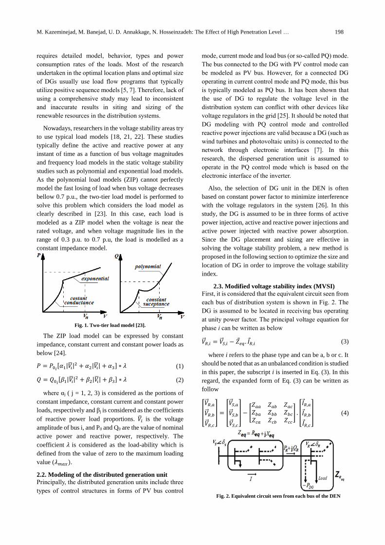
As the polynomial load models (ZIP) cannot perfectly

model the fast losing of load when bus voltage decreases

bellow 0.7 p.u., the two-tier load model is performed to

solve this problem which considers the load model as

clearly described in [23]. In this case, each load is

modeled as a ZIP model when the voltage is near the

rated voltage, and when voltage magnitude lies in the

range of 0.3 p.u. to 0.7 p.u, the load is modelled as a

constant impedance model.

Fig. 1. Two-tier load model [23].

The ZIP load model can be expressed by constant

impedance, constant current and constant power loads as

below [24].

𝑃 = 𝑃0𝑖[𝛼1|𝑉�̅�|

2 + 𝛼2|𝑉�̅�| + 𝛼3] ∗ 𝜆 (1)

𝑄 = 𝑄0𝑖[𝛽1|𝑉�̅�|

2 + 𝛽2|𝑉�̅�| + 𝛽3] ∗ 𝜆 (2)

where αj ( j = 1, 2, 3) is considered as the portions of

constant impedance, constant current and constant power

loads, respectively and βj is considered as the coefficients

of reactive power load proportions. �̅�𝑖 is the voltage

amplitude of bus i, and P0 and Q0 are the value of nominal

active power and reactive power, respectively. The

coefficient 𝜆 is considered as the load-ability which is

defined from the value of zero to the maximum loading

value (𝜆𝑚𝑎𝑥).

2.2. Modeling of the distributed generation unit

Principally, the distributed generation units include three

types of control structures in forms of PV bus control

mode, current mode and load bus (or so-called PQ) mode.

The bus connected to the DG with PV control mode can

be modeled as PV bus. However, for a connected DG

operating in current control mode and PQ mode, this bus

is typically modeled as PQ bus. It has been shown that

the use of DG to regulate the voltage level in the

distribution system can conflict with other devices like

voltage regulators in the grid [25]. It should be noted that

DG modeling with PQ control mode and controlled

reactive power injections are valid because a DG (such as

wind turbines and photovoltaic units) is connected to the

network through electronic interfaces [7]. In this

research, the dispersed generation unit is assumed to

operate in the PQ control mode which is based on the

electronic interface of the inverter.

Also, the selection of DG unit in the DEN is often

based on constant power factor to minimize interference

with the voltage regulators in the system [26]. In this

study, the DG is assumed to be in three forms of active

power injection, active and reactive power injections and

active power injected with reactive power absorption.

Since the DG placement and sizing are effective in

solving the voltage stability problem, a new method is

proposed in the following section to optimize the size and

location of DG in order to improve the voltage stability

index.

2.3. Modified voltage stability index (MVSI)

First, it is considered that the equivalent circuit seen from

each bus of distribution system is shown in Fig. 2. The

DG is assumed to be located in receiving bus operating

at unity power factor. The principal voltage equation for

phase i can be written as below

�⃗� 𝑅,𝑖 = �⃗� 𝑆,𝑖 − 𝑍 𝑒𝑞 . 𝐼 𝑅,𝑖 (3)

where i refers to the phase type and can be a, b or c. It

should be noted that as an unbalanced condition is studied

in this paper, the subscript i is inserted in Eq. (3). In this

regard, the expanded form of Eq. (3) can be written as

follow

[

�⃗� 𝑅,𝑎

�⃗� 𝑅,𝑏

�⃗� 𝑅,𝑐

] = [

�⃗� 𝑆,𝑎

�⃗� 𝑆,𝑏

�⃗� 𝑆,𝑐

] − [

𝑍𝑎𝑎 𝑍𝑎𝑏 𝑍𝑎𝑐

𝑍𝑏𝑎 𝑍𝑏𝑏 𝑍𝑏𝑐

𝑍𝑐𝑎 𝑍𝑐𝑏 𝑍𝑐𝑐

] . [

𝐼 𝑅,𝑎

𝐼 𝑅,𝑏

𝐼 𝑅,𝑐

] (4)

Fig. 2. Equivalent circuit seen from each bus of the DEN

Journal of Operation and Automation in Power Engineering, Vol. 7, No. 2, Oct. 2019 199

Substituting 𝐼 𝑅,𝑖 = (𝑃𝑅,𝑖+𝑗𝑄𝑅,𝑖

�⃗⃗� 𝑅,𝑖)∗

in the principal

voltage equation and separating the real and imaginary

parts, result:

𝑉𝑆,𝑖𝑉𝑅,𝑖𝐶𝑜𝑠(𝛿𝑖) = |𝑉𝑅,𝑖|2

+ [𝑅𝑒𝑞,𝑖(𝑃𝑅,𝑖 − 𝑃𝐷𝐺,𝑖)

+ 𝑋𝑒𝑞,𝑖𝑄𝑅,𝑖]

(5.a)

𝑉𝑆,𝑖𝑉𝑅,𝑖𝑆𝑖𝑛(𝛿𝑖) = [𝑋𝑒𝑞,𝑖(𝑃𝑅,𝑖 − 𝑃𝐷𝐺,𝑖) − 𝑅𝑒𝑞,𝑖𝑄𝑅,𝑖] (5.b)

where 𝛿𝑖 is the difference between the angles of the

sending bus voltage (VS) and the receiving bus voltage

(VR) for phase i (𝛿𝑖 = 𝛿𝑠,𝑖 − 𝛿𝑅,𝑖) . Also, in this analysis,

the first bus is considered as the reference bus with fixed

magnitude voltage. PR and QR are the total active and

reactive power received by the receiving bus in the

distribution system, respectively. Req and Xeq are also the

resistance and reactance equivalent to the radial

distribution line from the beginning of the feeder to the

power receiving bus, respectively calculated as follows:

(𝑃𝑠,𝑖 + 𝑗𝑄𝑠,𝑖) − (𝑃𝑅,𝑖 + 𝑗𝑄𝑅,𝑖)

= (𝑅𝑒𝑞,𝑖 + 𝑗𝑋𝑒𝑞,𝑖) ∗ |𝐼𝑖⃗⃗ |2

(6)

By calculating I�̅� = (�⃗⃗� 𝑆,𝑖−�⃗⃗� 𝑅,𝑖

𝑅𝑒𝑞,𝑖+𝑗𝑋𝑒𝑞,𝑖) and solving of above

equations, gives:

𝑅𝑒𝑞,𝑖 + 𝑗𝑋𝑒𝑞,𝑖

=[(𝑃𝑠,𝑖 − 𝑃𝑅,𝑖) + 𝑗(𝑄𝑆,𝑖 − 𝑄𝑅,𝑖)] ∗ |�⃗� 𝑆,𝑖 − �⃗� 𝑅,𝑖|

2

[(𝑃𝑠,𝑖 − 𝑃𝑅,𝑖)2+ (𝑄𝑆,𝑖 − 𝑄𝑅,𝑖)

2]

(7)

Eliminating the angle 𝛿𝑖 from Eq. (5.a) and Eq. (5.b),

|𝑉𝑅,𝑖|4+ {2[𝑅𝑒𝑞,𝑖(𝑃𝑅,𝑖 − 𝑃𝐷𝐺,𝑖) + 𝑋𝑒𝑞,𝑖𝑄𝑅,𝑖] − |𝑉𝑠,𝑖|

2} |𝑉𝑅,𝑖|

2

+{(𝑅𝑒𝑞,𝑖2 + 𝑋𝑒𝑞,𝑖

2 ) [(𝑃𝑅,𝑖 − 𝑃𝐷𝐺,𝑖)2+ 𝑄𝑅,𝑖

2]} = 0

(8)

More simplifications results:

|𝑉𝑅,𝑖|2

={|𝑉𝑠,𝑖|

2− 2[𝑅𝑒𝑞,𝑖(𝑃𝑅,𝑖 − 𝑃𝐷𝐺,𝑖) + 𝑋𝑒𝑞,𝑖𝑄𝑅,𝑖]} ± √∆

2

(9.a) (9.a)

∆= {2[𝑅𝑒𝑞,𝑖(𝑃𝑅,𝑖 − 𝑃𝐷𝐺,𝑖) + 𝑋𝑒𝑞,𝑖𝑄𝑅,𝑖] − |𝑉𝑠,𝑖|2}2

−4 {(𝑅𝑒𝑞,𝑖2 + 𝑋𝑒𝑞,𝑖

2 ) [(𝑃𝑅,𝑖 − 𝑃𝐷𝐺,𝑖)2+ 𝑄𝑅,𝑖

2]} (9.b)

Regarding the issue that |𝑉𝑅,𝑖|2≥ 0 ,

{|𝑉𝑠,𝑖|2− 2[𝑅𝑒𝑞,𝑖(𝑃𝑅,𝑖 − 𝑃𝐷𝐺,𝑖) + 𝑋𝑒𝑞,𝑖𝑄𝑅,𝑖]}

± √{2[𝑅𝑒𝑞,𝑖(𝑃𝑅,𝑖 − 𝑃𝐷𝐺,𝑖) + 𝑋𝑒𝑞,𝑖𝑄𝑅,𝑖] − |𝑉𝑠,𝑖|

2}2

−4 {(𝑅𝑒𝑞,𝑖2 + 𝑋𝑒𝑞,𝑖

2 ) [(𝑃𝑅,𝑖 − 𝑃𝐷𝐺,𝑖)2+ 𝑄𝑅,𝑖

2]}> 0

(10)

It can be understood that the first term of the left hand

side of (10) should be greater than zero,

{|𝑉𝑠,𝑖|2− 2[𝑅𝑒𝑞,𝑖(𝑃𝑅,𝑖 − 𝑃𝐷𝐺,𝑖) + 𝑋𝑒𝑞,𝑖𝑄𝑅,𝑖]} > 0

or, 2[𝑅𝑒𝑞,𝑖(𝑃𝑅,𝑖 − 𝑃𝐷𝐺,𝑖) + 𝑋𝑒𝑞,𝑖𝑄𝑅,𝑖] − |𝑉𝑠,𝑖|2< 0

(11)

Also, to obtain the practical result, Δ must be greater

or equal than zero (Δ ≥ 0). According to Eq. (9.a) and

Eq. (11), two acceptable voltages can be obtained for VR.

Fig. 3. Shows the concept of two voltages solution on the

PV curve.

{2[𝑅𝑒𝑞,𝑖(𝑃𝑅,𝑖 − 𝑃𝐷𝐺,𝑖) + 𝑋𝑒𝑞,𝑖𝑄𝑅,𝑖] − |𝑉𝑠,𝑖|2}2

≥ 4 {(𝑅𝑒𝑞,𝑖2 + 𝑋𝑒𝑞,𝑖

2 ) [(𝑃𝑅,𝑖 − 𝑃𝐷𝐺,𝑖)2+ 𝑄𝑅,𝑖

2]} (12)

Hence,

{2[𝑅𝑒𝑞,𝑖(𝑃𝑅,𝑖 − 𝑃𝐷𝐺,𝑖) + 𝑋𝑒𝑞,𝑖𝑄𝑅,𝑖] − |𝑉𝑠,𝑖|2}

≥ 2√(𝑅𝑒𝑞,𝑖2 + 𝑋𝑒𝑞,𝑖

2 ) [(𝑃𝑅,𝑖 − 𝑃𝐷𝐺,𝑖)2+ 𝑄𝑅,𝑖

2] (13.a)

{2[𝑅𝑒𝑞,𝑖(𝑃𝑅,𝑖 − 𝑃𝐷𝐺,𝑖) + 𝑋𝑒𝑞,𝑖𝑄𝑅,𝑖] − |𝑉𝑠,𝑖|2}

≤ −2√(𝑅𝑒𝑞,𝑖2 + 𝑋𝑒𝑞,𝑖

2 ) [(𝑃𝑅,𝑖 − 𝑃𝐷𝐺,𝑖)2+ 𝑄𝑅,𝑖

2] (13.b)

From Eq. (11) and Eq. (13), it can approve that Eq.

(13.b) is the only acceptable answer. Therefore, by

displacing the inequality of (13.b), we can obtain a

modified voltage stability index with the presence of DG

as follows,

𝑀𝑉𝑆𝐼𝑖 =2[𝑅𝑒𝑞,𝑖(𝑃𝑅,𝑖 − 𝑃𝐷𝐺,𝑖) + 𝑋𝑒𝑞,𝑖𝑄𝑅,𝑖] + 2√(𝑅𝑒𝑞,𝑖

2 + 𝑋𝑒𝑞,𝑖2 ) [(𝑃𝑅,𝑖 − 𝑃𝐷𝐺,𝑖)

2+ 𝑄𝑅,𝑖

2]

|𝑉𝑠,𝑖|2 ≤ 1 (14)

The distribution system studied will be stable when the

value of defined index for each bus in all phases is less

than one (0≤MVSIi <1). This voltage stability indicator

is dimensionless and as a result, both actual and per-unit

values can be used.

3. OPTIMIZATION TECHNIQUE

To maximize the benefits of using dispersed generation

units in the distribution system, proper size and optimal

DG placement are needed. Due to outstanding aspects of

ICA such as high speed convergence, this optimization

M. Kazeminejad, M. Banejad, U. D. Annakkage, N. Hosseinzadeh: The Effect of High Penetration Level … 200

method is used along with the backward/forward sweep

load flow in unbalanced radial distribution electricity

network [27-28].

Fig. 3. Two voltage solutions and PV curve.

3.1. Problem formulation for siting and sizing of DG

In this section, the problem of finding the optimal size

and proper location for DG installation is addressed by

improving the voltage stability indicator presented in the

previous section regarding the reduction of power losses

in the distribution system. For this purpose, the DG is

assigned to the buses which have the highest values of

the voltage stability index. In the algorithm illustraded in

flowchart of Fig.4, the size of DG is increased

incrementally to achieve the lowest value of the objective

function.

3.2. The proposed objective function

In this study, the proposed objective function is to

optimize the DG capacity by minimizing the total power

loss of power lines and improving the voltage stability

index simultaneously, as follows:

𝑓 = 𝑚𝑖𝑛 {(∑ (𝑅𝑘,𝑎|𝐼�̅�,𝑎|2+ 𝑅𝑘,𝑏|𝐼�̅�,𝑏|

2+𝑛𝑏

𝑘=1

𝑅𝑘,𝑐|𝐼�̅�,𝑐|2)) + 𝑀𝑉𝑆𝐼𝑖}

(15)

Subject to

0 ≤ 𝑃𝐷𝐺 ≤25

100∑𝑃𝐿𝑜𝑎𝑑,𝑗

𝑛

𝑗=1

(16)

where nb is the number of the distribution system

branches, n is the number of buses, PDG is the active

power injected by the distributed generation unit and

PLoad is the active power loads connected to each bus. The

voltage magnitude in the beginning of the feeder

(considered as an infinite bus) is set to 1.00(p.u.) with an

angle of 0 degree. The voltage range for other buses are

considered as

𝑉𝑗,𝑚𝑖𝑛≤ 𝑉𝑗 ≤ 𝑉𝑗,𝑚𝑎𝑥

, 𝑗 = 2, …𝑛 (17)

The voltage constraints for 𝑉𝑗,𝑚𝑎𝑥 and 𝑉𝑗,𝑚𝑖𝑛

are

1.05 (p.u.) and 0.9(p.u.), respectively.

3.3. The procedure for siting and sizing of DG

After applying the backward/forward sweep load flow

method and determining the critical buses near to the

voltage instability, incremental step size of DG for

critical buses are implemented separately. After

completing the steps for all buses that are prone to DG

installation, the selected bus with the optimum size of DG

will be chosen under the lowest value of the proposed

objective function from the database. At this stage, it is

assumed that DG unit has a unit power factor.

Fig. 4. Optimization schedule flowchart for allocation and size of

DG

4. SIMULATION AND RESULT

In order to verify the correctivenes of the proposed index

in voltage stability assessment in comparison to couple

of different indicators, a simulation has been performed

on the two bus equivalent system shown in Fig. 2.

The fast voltage stability index (FVSI) given in Ref.

[29] is presented as (18), which depends only to reactive

power load.

𝐹𝑉𝑆𝐼 =4|𝑍𝑒𝑞,𝑖|

2𝑄𝑅,𝑖

𝑋𝑒𝑞,𝑖|𝑉𝑆,𝑖|2 (18)

Therefore, with variation of the active power load in

receiving buses (especially in DGs having unit power

factor), this method cannot be used. Hence, FVSI will not

be applicable to be used in voltage analysis in DNO.

Also, the power stability index (PSI) which was defined

Journal of Operation and Automation in Power Engineering, Vol. 7, No. 2, Oct. 2019 201

by Amman [30] has some inaccuracies.

𝑃𝑆𝐼 =4𝑅𝑒𝑞,𝑖(𝑃𝑅,𝑖 − 𝑃𝐷𝐺,𝑖)

|𝑉𝑆,𝑖|2𝑐𝑜𝑠2(𝜃𝑖 − 𝛿𝑖)

(19)

where 𝛿𝑖 = 𝛿𝑆,𝑖 − 𝛿𝑅,𝑖 and 𝜃𝑖 = arctan (𝑋𝑒𝑞,𝑖

𝑅𝑒𝑞,𝑖).

PSI varies from 0 (no loading) to 1 (collapse point)

when (𝑃𝑅,𝑖 − 𝑃𝐷𝐺,𝑖) > 0 . If (𝑃𝑅,𝑖 − 𝑃𝐷𝐺,𝑖) ≤ 0 , PSI

becomes negative or zero, which shows the system

always has a stable voltage. The comparison between

these indicators and proposed MVSI is given as follow.

In Fig. 2, it is assumed that 𝑉𝑆∡𝛿𝑆 = 1.00∡0.0 (𝑝. 𝑢. ),

and as an example, impedance assumed as 𝑅𝑒𝑞 + 𝑗𝑋𝑒𝑞 =

0.05 + 𝑗0.1 (𝑝. 𝑢. ). The values of load demand at load

initial condition are assumed as 𝑃𝑅 + 𝑗𝑄𝑅 = 0.5 +

𝑗1.0 (𝑝. 𝑢. ) . Tables 1, 2 and 3 present two voltage

solutions at the receiving bus for each iteration, which

express the PV curve. The three voltage indicators MVSI,

FVSI and PSI are calculated when the load is gradually

increased. 𝜆 represents as load-ability factor with regard

to its initial value of load. Table 1 shows the results when

both active and reactive power loads are increased with a

constant power factor. It can be seen that at 𝜆 = 2.00, all

indicators work properly. Table 2 shows the result when

only the active power loads are increased. It can be

understood that the FVSI is constant for all load-ability

factors and it is not proper to use it for voltage stability.

Also, the PSI reaches to its maximum value (voltage

collapse point, PSI=1.00) at 𝜆 = 3.845 ; whereas the

magnitude of two voltages solution at the receiving bus

on PV curve still not reached to nose point. Table 3 shows

the result when only the reactive power loads are

increased. It is described that FVSI reaches to its

maximum value with 𝜆 = 2.00 ; in while nose point

doesn’t happen. Also, the PSI doesn’t work correctly and

has an essential flaw; where the two voltage solutions

reach together as a nose point of PV curve, but the value

of PSI is 0.8834.

Table 1. DNS load-ability when both active and reactive power

loads are increased with constant power factor

𝝀

PV Curve

MVSI PSI

[30]

FVSI

[29] VHigh(p.u.) VLow(p.u.)

1.0000 0.8535 0.1464 0.5000 0.5000 0.5000

1.4776 0.7555 0.2444 0.7388 0.7388 0.7388

1.8927 0.6158 0.3842 0.9463 0.9463 0.9463

2.0000 0.5000 0.5000 1.0000 1.0000 1.0000

Table 2. DNS load-ability only by increasing of active power load

𝝀 PV Curve

MVSI PSI

[30]

FVSI

[29] VHigh(p.u.) VLow(p.u.)

1.0000 0.8535 0.1464 0.5000 0.5000 0.5000

1.8927 0.8185 0.1880 0.6025 0.7714 0.5000

2.6521 0.7816 0.2376 0.7040 0.9121 0.5000

3.8443 0.6981 0.3470 0.8767 1.0000 0.5000

4.6602 0.5324 0.5324 1.0000 --- 0.5000

Table 3. DNS load-ability only by increasing of reactive power

load

𝝀 PV Curve

MVSI PSI

[30]

FVSI

[29] VHigh(p.u.) VLow(p.u.)

1.0000 0.8535 0.1464 0.5000 0.5000 0.5000

1.3125 0.8059 0.1948 0.6266 0.5414 0.6562

1.7011 0.7325 0.2706 0.7867 0.6130 0.8505

2.0000 0.6519 0.3535 0.9110 0.7025 1.0000

2.2132 0.5037 0.5037 1.0000 0.8834 ---

4.1. The Case study

The studied system is an unbalanced IEEE 13 Bus Test

Feeder with 4.16 kV and a total Spot Load of 3266 kW,

1986 kVAr and distributed load of 200 kW, 116 kVAr,

one tap changer transformer and one transformer 4.16

kV/0.48 kV and also, 2 capacitive banks in buses 13 and

10 according to fig.5. The details of power lines and

loads data are presented in Ref. [31].

In this study, some assumptions have been made for

simulations. Take, for example, ignoring limited thermal

capacity and the susceptance of lines. In addition, it is

assumed that the magnitude voltage of the first bus is 1.00

p.u. Also, the position of transformer taps are included

for each phase individually regarding that taps range will

be 10 steps.

4.2. The effect of transformer taps on voltage stability

Figure 6 shows the voltage profile of phases A to C for

three cases; normal load, increasing the load-ability by

fixing the transformer taps obtained from the previous

state (the values of 6, 5 and 6 for phases A, B and C,

respectively), and increasing the load-ability in condition

of changing the transformer taps. The results describe the

voltage instability condition due to an increase in load-

ability to (𝜆𝑚𝑎𝑥 = 1.3 ), while the taps position of

transformer are fixed to 6, 5, 6 for three phases. Also,

considering the flexibility of the transformer tap changer

in the specified range, it can be seen that the voltage

profile and therefore the voltage stability margin are

significantly improved.

Figure 7 shows the status of the modified voltage

stability index for all three proposed cases. It is shown

that when the maximum load-ability condition occurs,

the index amount reaches its critical value, i.e., the value

one in the critical bus 7, which means that the voltage

collapse occurred.

M. Kazeminejad, M. Banejad, U. D. Annakkage, N. Hosseinzadeh: The Effect of High Penetration Level … 202

Fig. 6. voltage profiles of three phase for maximum load-ability; i) Phase A , ii) Phase B , iii) Phase C

Fig. 5. IEEE13bus distribution test system

Fig. 7. Three-phase voltage stability index for maximum load-

ability

4.3. The effect of optimized DG siting on the voltage

stability

Based on the optimization algorithm defined in the

section three, the bus number 13 is identified as the best

location for DG installation. Figure 8 shows the power

loss reduction due to optimal DG siting in bus 13 in

which the total active power loss is decreased

approximately 40%. Table 4 shows the optimal DG size

and total losses of the whole system containing the

transformer taps in each phase. It can be observed that the

total amount of active power loss decreases from

213.42MW to 127.46MW as transformer tap is set to 5

for all phases. Also, the voltage profile for the phase B is

shown in Fig. 9 excluding the DG and with optimum size

of DG in normal load case that is observed with

considering the optimal DG, the voltage profile is

significantly improved.

Fig. 8. System power losses with / without optimal DG

Journal of Operation and Automation in Power Engineering, Vol. 7, No. 2, Oct. 2019 203

Fig. 9. Voltage profile of phase B with / without DG optimum size

Fig. 11. The effect of the DG types on the load-ability for Phase A

Table 4. System power losses with / without DG and transformer taps status

Transformer taps status Reactive power loss

(kVar) Active power loss

(kW) Size (kW)

Bus

Number

Phase c Phase b Phase a

6 5 6 576.61 213.42 --- Without DG

5 5 5 340.11 127.46 288.83 13 With optimal DG

Fig. 10. The load-ability effect on the voltage profile (i) phase A, and (ii) phase B; with / without DG

The voltage profiles in Fig. 10 illustrate a comparison of

the impact of the load-ability for three cases; normal load

conditions with and without the DG installation for the

two phases A and B. Without DG, the maximum load-

ability reaches to 𝜆𝑚𝑎𝑥 = 1.3 with a change in the tap

position of the transformers to 8, 7 and 8 for A, B and C

phases, respectively. It is also shown that with the

optimized DG siting in Bus 13, the system load-ability

increases to 𝜆𝑚𝑎𝑥 = 1.51.

The influence of the DG types on load-ability of phase

A is depicted in Fig. 11 for three different modes of DG

performance, active power injection with unit power

factor (PF = 1), active and reactive power injections with

0.9 lagging PF and active power injected with reactive

power absorption with 0.9 leading PF. The results

demonstrate that if the DG is capable of injecting both

active and reactive power simultaneously, the load-

ability increases significantly to 𝜆𝑚𝑎𝑥 = 1.71. Also, if

the DG operates in a lag power factor mode, a

considerable reduction in the system load-ability

occur ( 𝜆𝑚𝑎𝑥 = 1.34).

4.4. The effect of DG high penetration level on voltage

stability

In order to study the penetration level of distributed

generations on the voltage stability in DEN, two critical

buses 7 and 13 are separately selected for DG installation.

In this case, the DG size is increased up to 80% of the

total demanded load by step size of 5%. Then, for each

step, the maximum load-ability and the sensitivity of

load-ability to penetration level are presented. In order to

analyze the sensitivity of load-ability to penetration level,

the maximum load-ability difference for the two closest

DG penetration levels per the maximum load-ability

without DG installation is calculated. The tap positions

of transformer is fixed to 6, 5, 6 for each step.

∆𝜆 =𝜆𝑚𝑎𝑥(𝑖) − 𝜆𝑚𝑎𝑥(𝑖 − 1)

𝜆𝑚𝑎𝑥(𝑊𝑖𝑡ℎ𝑜𝑢𝑡_𝐷𝐺) (20)

𝜆𝑚𝑎𝑥 is the maximum load-ability and i refers to the step

increment of DG penetration level in each step.

According to Table 5, the maximum load-ability (𝜆𝑚𝑎𝑥)

rises by increasing the DG penetration level in

distribution system. It can also be seen that for increasing

the penetration level above 55%, the sensitivity of load-

ability tends to decrease significantly in comparison with

the lower DG penetration levels.

It means that if the DG is installed in critical bus 13,

with an increase in penetration level to 45% of the total

demanded load, the load-ability sensitivity reaches the

highest rate equal to 7.69% compared with 40% of

penetration level. Also, for the penetration level higher

than 60% of the total demanded power, the sensitivity

M. Kazeminejad, M. Banejad, U. D. Annakkage, N. Hosseinzadeh: The Effect of High Penetration Level … 204

load-ability decreases. It is obtained that the sensitivity

load-ability for 60% of penetration level is equal 6.92%.

These results describe that the slope of maximum load-

ability decreases by growing up the DG penetration level

and the use of DG in these circumstances may be not

justified.

Table 5. System load-ability and the DG penetration level at bus 13

Active power loss

(kW) ∆𝝀(%) 𝝀𝒎𝒂𝒙 DG penetration

level (%) 4.3239 0 1.3 0

4.3536 4.62 1.36 5 4.5393 6.15 1.44 10 4.5879 5.38 1.51 15 4.6923 6.15 1.59 20 4.8528 6.92 1.68 25 4.9856 6.92 1.77 30 5.1024 6.92 1.86 35 5.2189 6.92 1.95 40 5.4406 7.69 2.05 45 5.7077 7.69 2.15 50 6.0534 7.69 2.25 55 6.4203 6.92 2.34 60 6.8371 6.15 2.42 65 7.2160 4.62 2.48 70 7.7973 4.62 2.54 75 8.2188 2.31 2.57 80

Table 6. System load-ability and the DG penetration level at bus 7

Active power loss

(kW) ∆𝝀(%) 𝝀𝒎𝒂𝒙 DG penetration

level (%) 4.3239 0 1.3 0

4.3988 4.62 1.36 5 4.5324 5.38 1.43 10 4.7220 6.15 1.51 15 4.8703 6.15 1.59 20 4.9778 6.15 1.67 25 5.1411 6.92 1.76 30 5.2695 6.92 1.85 35 5.4636 7.69 1.95 40 5.6412 7.69 2.05 45 5.8183 7.69 2.15 50 6.0171 7.69 2.25 55 6.2667 7.69 2.35 60 6.4006 6.15 2.43 65 6.6502 6.15 2.51 70 6.8404 4.62 2.57 75 7.0979 3.85 2.62 80

The results of the sensitivity load-ability analysis for

increasing the DG penetration level installed in the

critical bus 7 are tabulated in table 6. It can be seen that

the maximum sensitivity load-ability reaches to 40 % of

penetration level (7.69%). This rate has been reduced for

penetration levels above 60%, and the amount of

sensitivity load-ability has decreased to 6.15% in 65% of

penetration level.

4.5. The interaction effect of the transmission

system on the distribution system load-

ability

The transmission and distribution systems are physically

connected to each other, but they are typically studied

separately in the analysis of voltage stability assessment.

Table 7 shows the interactive effect of the transmission

system on the distribution system load-ability. In this

analysis, it is assumed that the initial voltage of the

distribution feeder connected to the transmission network

decreases to 0.95 p.u. due to some constraints of the

transmission system.

The first row of table 7 describe that the system load-

ability increases from 1.3 to 1.51 by considering the DG

unit and with the change in transformer tap positions to

8, 7 and 8 for each phase, individually. It is also observed

that the load-ability decreases due to a voltage drop from

1.3 to 1.19, when the DG is not considered (column one).

In this case, the transformer taps significantly increase in

order to maintain the distribution voltage profile in the

desired range. Although, in the presence of DG the load-

ability has not made any significant change (column

two), the tap positions of transformer increased to 9, 9

and 10 for each phase in order to maintain normal

condition of voltage stability in the system.

Table 7. The interaction effect of the transmission system on the distribution system load-ability

5. CONCLUSIONS

In this research, a modified voltage stability index

(MVSI) presented in an unbalanced three-phase DENs in

presence of distributed generation units. It has been

shown that by considering load model and best size of

DG, a significant effect on the voltage profile and voltage

stability in DEN can be achieved. In order to improve the

voltage stability index and reduce the effects of

transformer taps in the distribution system, the ICA

optimization technique has been used to determine the

sizing and siting of DG with loss reduction. Furthermore,

the influence of DG penetration level on the system load-

ability margin is analyzed. It has been described that the

load-ability margin can be improved by DG penetration

level. However, the speed rate of load-ability was

significantly reduced with respect to increase in high DG

With optimal DG (PF=0.9 lag) With optimal DG (PF=1) Without DG Muximum Load-ability

(𝝀𝒎𝒂𝒙) Phase c Phase b Phase a Phase c Phase b Phase a Phase c Phase b Phase a

1.34 1.51 1.3 V=1 p.u.

8 7 8 8 7 8 6 5 6 Transformer taps status

1.36 1.52 1.19 V=0.95 p.u.

10 9 9 10 9 9 9 8 9 Transformer taps status

Journal of Operation and Automation in Power Engineering, Vol. 7, No. 2, Oct. 2019 205

penetration levels. Moreover, since the effect of the

transmission system constraints is typically ignored on

the voltage stability studies in the distribution system, the

impact of the distribution system load-ability on the

transmission system has been investigated. It has been

shown that the voltage reduction of the transmission

system has a negative effect on both the load-ability and

the transformer tap positions in distribution system.

REFERENCES [1] Y. M. Atwa, E. F. El-Saadany, M. M. A. Salama, R.

Seethapathy, “Optimal renewable resources mix for

distribution system energy loss minimization,” IEEE

Trans. Power Syst., vol. 25, no. 1, pp. 360-370, 2010.

[2] M. Ettehadi, H. Ghasemi, S. Vaez-Zadeh, “Voltage

Stability-Based DG Placement in Distribution electricity

networks,” IEEE Trans. Power Del., vol. 28, no. 1, 2013.

[3] S. Ghaemi, K. Zare, “A New Method of Distribution

Marginal Price Calculation in Distribution Networks by

Considering the Effect of Distributed Generations

Location on Network Loss”, J. Oper. Autom. Power Eng.,

vol. 5, No. 2, Dec. 2017, Pages: 171-180.

[4] R. walling, et. al., “summary of distributed resources

impact on power delivery systems,” IEEE Trans. Power

Del., vol. 23, 2008.

[5] M. Thomson, D. G. Infield, “Network power flow analysis

for a high penetration of distributed generation,” IEEE

Trans. Power syst., vol. 22, pp. 1157-1162, 2007.

[6] P.P. Barker, R.W. de Mello, “Determining the impact of

Distributed generation on power systems: Part 1 —radial

distribution systems,” Proc. IEEE Power Eng. Soc.

Summer Meeting, pp. 1645-1654, 2000.

[7] R. S. Al Abri, E. F. El-Saadany; Y. M. Atwa, “optimal

placement and sizing method to improve the voltage

stability margin in a distribution system using distributed

generation,” IEEE Trans. Power syst., vol. 28, 2013.

[8] P. Aristidou, G. Valverde, T. V. Cutsem, “Contribution of

Distribution Network Control to Voltage Stability: A Case

Study”, IEEE Trans. Smart Grid, 2017, vol. 8, no. 1, pp:

106 –116.

[9] R. A. Walling, R. Saint, R. C. Dugan, J. Burke, L. A.

Kojovic, “Summary of Distributed Resources Impact on

Power Delivery Systems”, IEEE Trans. Power Del., vol.

23, no. 3, JULY 2008.

[10] D. Guiping, J. Xu, “A new index of voltage stability

considering Distribution electricity network,” IEEE Asia-

Pac. Power Energy Eng. Conf., 2009.

[11] T. Van Custem, “voltage stability of electic powet

systems,” Springer Sci. Bus. Media, vol. 441, 1998.

[12] K.Liu, W. Sheng, L. Hu, Y. Liu, X. Meng, D. Jia,

“Simplified probabilistic voltage stability evaluation

considering variable renewable distributed generation in

distribution systems”, IET Gener. Transm. Distrib., 2015,

vol. 9, no. 12, pp. 1464–1473.

[13] X. Ran, S. Miao, “Probabilistic evaluation for static

voltage stability for unbalanced three-phase distribution

system”, IET Gener. Transm. Distrib., 2015, vol. 9, no. 14,

pp. 2050–2059.

[14] F. Namdari, L. Hatamvand, N. Shojaei, H. Beiranvand,

“Simultaneous RPD and SVC Placement in Power

Systems for Voltage Stability Improvement Using a Fuzzy

Weighted Seeker Optimization Algorithm”, J. Oper.

Autom. Power Eng., vol. 2, no. 2, pp. 129-140, 2014.

[15] S. Derafshi Beigvand, H. Abdi, S. N. Singh, “Voltage

stability analysis in radial smart distribution grids,” IET

Gener. Transm. Distrib., vol. 11 no. 15, pp. 3722-3730,

2017.

[16] M. Chakravorty, D. Das, “Voltage stability analysis of

radial distribution networks,” Elsevier Sci. Ltd., Electr.

Power Energy Syst., 23 (2001) 129-135.

[17] T. Zabaiou, L. A. Dessaint, I. Kamwa, “preventive control

approach for voltage stability improvement using voltage

stability constrained optimal power flow based on static

line voltage stability indices,” IET Gener. Transm.

Distrib.., vol. 8, pp. 924-934, 2014.

[18] M. Banejad, M. Kazeminejad, “Load effects on voltage

stability in Distribution electricity network with

considering of distributed generation,” IEEE conf. 58th Int.

Sci. conf. power Electr. Eng., 2017.

[19] K. A. Birt, J. J. Graffy, A. H. El-Abiad, “Three phase load

flow program,” IEEE Trans. Power App. Syst., vol. 95, no.

1, 1976.

[20] X. P. Zhang, “Fast three phase load flow methods,” IEEE

Trans. Power syst., vol. 11, no. 3, 1996.

[21] D. Singh, R. K. Misra, De. Singh, “Effect of load models

in distributed generation planning,” IEEE Trans. Power

syst., vol. 22, no. 4, 2007.

[22] T. Gozel, M.H. Hocaoglu, U. Eminoglu, A. Balikci,

“optimal placement and sizing of distributed generation on

radial feeder with different static load models,” Int. Conf.

Future Power Syst., 2005.

[23] J. Machowski, “Power System Dynamics Stability and

Control,” John Wiley and Sons, Ltd, Second Edition, 2008.

[24] IEEE Task Force on Load Representation for Dynamic

Performance, “Bibliography on load models for power

flow and dynamic performance simulation,” IEEE Trans.

Power syst., vol. 10, 1995.

[25] IEEE Standard for Distributed Resoursec “Interconnected

with Electric Power Systems,” IEEE p1547 std. 2002.

[26] R. A. Walling, et. Al. “Summary of distributed resources

impact on power delivery systems,” IEEE Trans. Power

Del., vol. 23, no. 3, 2008.

[27] M. Abdel-Akher, “Voltage stability analysis of

unbalanced distribution systems using backward/forward

sweep load-flow analysis method with secant predictor”,

IET Gener. Transm. Distrib., 2013, vol. 7, no. 3, pp. 309-

317.

[28] A. Soroudi M. Ehsan, “Imperialist competition algorithm

for distributed generation connections”, IET Gener.

Transm. Distrib., 2012, Vol. 6, Iss. 1, pp. 21–29.

[29] Musirin, T. K. Abdul Rahman, “On-Line Voltage Stability

Based Contingency Ranking Using Fast Voltage Stability

Index (FVSI),” IEEE/PES Transm. Distrib. Conf.

Exhibition, Yokohama, Japan, 6-10 Oct. 2002.

[30] M.M. Aman, G.B. Jasmon, H. Mokhlis, A.H.A. Bakar,

“Optimal placement and sizing of a DG based on a new

power stability index and line losses”, Elsevier Sci.Ltd.,

Electr. Power Energy Syst., vol. 43 pp.1296-1304, 2012.

[31] IEEE PES Distribution Systems Analysis Subcommittee

Radial Test Feeders. http://sites.ieee.org/pestestfeeders/re-

sources/ .