the effect of environmental factors on the … · the effect of environmental factors on the...
TRANSCRIPT

THE EFFECT OF ENVIRONMENTAL FACTORS
ON THE IMPLEMENTATION OF THE MECHANISTIC-EMPIRICAL
PAVEMENT DESIGN GUIDE (MEPDG)
George Abraham Dzotepe
Graduate Research Assistant
Department of Civil and Architectural Engineering
University of Wyoming
Dr. Khaled Ksaibati, Ph.D., P.E.
Director
Wyoming Technology Transfer Center
July 2011

Acknowledgements
The authors would like to thank the Mountain-Plains Consortium (MPC) for providing funding for this
research study and also the staff of the Water Resources Data System (WRDS) at the University of
Wyoming for providing the available weather data. They also wish to thank the Wyoming Department of
Transportation (WYDOT) for providing other input data for the study.
Disclaimer
The contents of this report reflect the views of the authors, who are responsible for the facts and the
accuracy of the information presented. This document is disseminated under the sponsorship of the
Department of Transportation, University Transportation Centers Program, in the interest of information
exchange. The United States Government assumes no liability for the contents or use thereof.
North Dakota State University does not discriminate on the basis of age, color, disability, gender expression/identity, genetic information, marital status, national origin, public assistance status, sex, sexual orientation, status as a U.S. veteran, race or religion. Direct inquiries to the Vice President for Equity, Diversity and Global Outreach, 205 Old Main, (701)231-7708.

ABSTRACT
Current pavement design based on the AASHTO Design Guide uses an empirical approach from the
results of the AASHO Road Test conducted in 1958. To address some of the limitations of the original
design guide, AASHTO developed a new guide: Mechanistic Empirical Pavement Design Guide
(MEPDG). This guide combines the mechanistic and empirical methodology by making use of
calculations of pavement responses such as stress, strains, and deformations using site specific inputs
from climate, material, and traffic properties. With the new guide, various implementation challenges
need to be overcome by agencies wanting to facilitate its use. In this respect, the MEPDG is currently
undergoing several validation and calibration research studies, which are in the areas of materials, climate
and traffic characteristics. It is anticipated that the findings from the various research studies will facilitate
the implementaion of the MEPDG nationwide. This study summarizes the challenges that are likely to
impede implementation of the MEPDG within the Northwest Region and how these can be overcome.
The study also investigates the effects of climate variables on the predicted pavement performance
indicators and, in addition, evaluates the adequacy of using interpolated climate data on pavement
performance in the state of Wyoming.


TABLE OF CONTENTS 1 INTRODUCTION ................................................................................................................................ 1
1.1 Background ................................................................................................................................... 1
1.2 Problem Statement ........................................................................................................................ 3
1.3 Objectives ..................................................................................................................................... 4
1.4 Report Organization ..................................................................................................................... 4
2 LITERATURE REVIEW .................................................................................................................... 5
2.1 Background ................................................................................................................................... 5
2.2 MEPDG Design Process ............................................................................................................... 6
2.3 MEPDG Performance Indicators .................................................................................................. 7
2.3.1 Alligator Cracking (Bottom-Up Cracking) ........................................................................ 7
2.3.2 Longitudinal Cracking (Surface-down Fatigue Cracking) ................................................ 7
2.3.3 Transverse Cracking (Thermal Cracking) ......................................................................... 7
2.3.4 Rutting ............................................................................................................................... 7
2.3.5 International Roughness Index (IRI) ................................................................................. 7
2.4 Performance Prediction Equations for Flexible Pavements ......................................................... 8
2.5 Design Criteria and Reliability ..................................................................................................... 8
2.6 Calibration .................................................................................................................................... 9
2.7 MEPDG Inputs ........................................................................................................................... 10
2.7.1 Traffic Data ...................................................................................................................... 10
2.7.1.1 Hierarchal Approach to Traffic Inputs ................................................................ 11
2.7.1.2 Traffic Elements .................................................................................................. 11
2.7.2 Climate/Environment and EICM ..................................................................................... 14
2.7.2.1 Virtual Weather Stations ..................................................................................... 14
2.7.3 Material Data ................................................................................................................... 15
2.7.3.1 Resilient Modulus and Unbound Layers ............................................................. 15
2.7.3.2 Hierarchal Approach to Material Inputs.............................................................. 16
2.8 Section Summary ........................................................................................................................ 17
3 REGIONAL IMPLEMENTATION OF MEPDG ........................................................................... 19
3.1 Background ................................................................................................................................. 19
3.2 User Group Meeting ................................................................................................................... 19
3.2.1 National Implementation Plan ......................................................................................... 20
3.2.2 Regional Implementation Plan ........................................................................................ 20
3.2.2.1 Washington DOT ................................................................................................ 20

3.2.2.2 Oregon DOT ....................................................................................................... 21
3.2.2.3 South Dakota DOT .............................................................................................. 21
3.2.2.4 Wyoming DOT ................................................................................................... 22
3.2.3 Regional Research Needs ................................................................................................ 23
3.2.3.1 Traffic Data Characteristics ................................................................................ 24
3.2.3.2 Climate/Environment Factors ............................................................................. 24
3.2.3.3 Materials Characterization .................................................................................. 25
3.2.3.4 Pavement Performance........................................................................................ 25
3.2.3.5 Calibration and Validation .................................................................................. 25
3.2.4 Challenges and Limitations to Implementation Efforts ................................................... 26
3.2.5 Benefits of Implementing the MEPDG ........................................................................... 27
3.3 Section Summary ........................................................................................................................ 29
4 DATA COLLECTION ....................................................................................................................... 30
4.1 Introduction ................................................................................................................................ 30
4.2 Design Inputs .............................................................................................................................. 30
4.2.1 Traffic Input Data ............................................................................................................ 30
4.2.2 Pavement Material Data .................................................................................................. 31
4.2.2.1 Primary System ................................................................................................... 31
4.2.2.2 Secondary System ............................................................................................... 32
4.2.2.3 Interstate System ................................................................................................. 33
4.2.2.4 Binder Grades ..................................................................................................... 33
4.3 Climate Data ............................................................................................................................... 34
4.3.1 Virtual Weather Stations Generation ............................................................................... 36
4.4 Section Summary ........................................................................................................................ 36
5 DATA ANALYSIS ............................................................................................................................. 37
5.1 Introduction ................................................................................................................................ 37
5.2 Annual Climate Statistics ........................................................................................................... 37
5.3 Performance Distresses ............................................................................................................... 38
5.3.1 Interstate System .............................................................................................................. 38
5.3.1.1 Performance Distresses for Different Binder Types ........................................... 38
5.3.1.2 Climate Analysis ................................................................................................. 42
5.3.1.3 Virtual Climate Analysis ..................................................................................... 47
5.4 Statistical Analysis ..................................................................................................................... 51
5.4.1 Regression Models for P-values Calculations ................................................................. 52
5.4.1.1 Explanation of Regression terms ........................................................................ 52
5.4.1.2 Coefficient of Multiple Determination (R2 and Adjusted R2) ............................. 54
5.4.1.3 Coefficient of Correlation ................................................................................... 54
5.4.2 Interstate System .............................................................................................................. 54
5.4.2.1 Confidence Intervals and P-values Calculations on Differences ........................ 54
5.4.2.2 Confidence Intervals and P-values Calculations using Percentage Change ........ 57

5.4.3 Primary System ................................................................................................................ 59
5.4.4 Secondary System ............................................................................................................ 63
5.5 Summary of Statistical Analysis ................................................................................................. 66
5.6 Section Summary ........................................................................................................................ 67
6 CONCLUSIONS AND RECOMMENDATIONS ........................................................................... 69
6.1 Conclusions ................................................................................................................................ 69
6.2 Recommendations ...................................................................................................................... 70
REFERENCES .......................................................................................................................................... 71
APPENDICES ........................................................................................................................................... 73
APPENDIX A1: Flexible Pavement Performance Prediction Equations ............................................... 75
APPENDIX A2: MEPDG Data Input Screens........................................................................................ 79
APPENDIX B1: Pavement Database Surface/Base Type Designations ................................................. 91
APPENDIX B2: Extract From Primary Road PMS ................................................................................ 93
APPENDIX B3: Extract From Secondary Road PMS ............................................................................ 99
APPENDIX B4: Extracts from I-80 PMS ............................................................................................. 100
APPENDIX B5: WYDOT Binder Grades ............................................................................................ 105
APPENDIX C1: Predicted Distresses for Different Binder Grades ..................................................... 107
APPENDIX D1: Predicted Distresses for Interstate System ................................................................ 111
APPENDIX D2: Annual Climate Statistics .......................................................................................... 125
APPENDIX D3: Predicted Distresses for Primary System .................................................................. 135
APPENDIX D4: Predicted Distresses for Secondary System .............................................................. 149
APPENDIX E1: Interstate Scatter Plots ............................................................................................... 163

LIST OF TABLES
Table 2.1 Recommended Threshold Design Values (AASHTO 2008) ....................................................... 8
Table 2.2 Reliability Levels Roadway Classifications (AASHTO 2008) .................................................... 9
Table 2.3 MEPDG Traffic Inputs .............................................................................................................. 12
Table 2.4 FWHA System of Vehicle Classification (Source: www.fhwa.dot.gov) ................................... 13
Table 2.5 Major Material Input Considerations (Wang et al., 2007) .......................................................... 18
Table 3.1 SDOT Implementation Term Plans ........................................................................................... 22
Table 4.1 Traffic Input Data ....................................................................................................................... 31
Table 4.2 Weather Station Locations in Wyoming .................................................................................... 34
Table 5.1 Annual Climate Statistics for Actual Stations ............................................................................ 37
Table 5.2 General Traffic Inputs ................................................................................................................ 38
Table 5.3 Design Limiting Values ............................................................................................................. 38
Table 5.4 Predicted Pavement Distresses Using Different Binder Types at Big Piney ............................. 39
Table 5.5 Summary of Performance Distresses Using PG52-28 ............................................................... 43
Table 5.6 Summary of Performance Distresses Using PG76-28 ............................................................... 44
Table 5.7 Pavement Performance –Virtual Station Using All Generated Stations (PG52-28) .................. 48
Table 5.8 Climate Statistics Using All Neighboring Stations .................................................................... 49
Table 5.9 Pavement Distresses Using Similar Elevations (PG52-28) ....................................................... 50
Table 5.10 Climate Statistics Using Similar Elevations ............................................................................. 51
Table 5.11 Confidence Intervals for Performance Parameters using Differences ...................................... 55
Table 5.12 Confidence Intervals for Climate Statistics using Differences ................................................. 55
Table 5.13 P-Values Calculations Using Differences ................................................................................ 56
Table 5.14 Significant Climate Variables for Interstate System ................................................................ 57
Table 5.15 Confidence Intervals on Percentage Change ........................................................................... 58
Table 5.16 Confidence Interval Using Percentage Change ....................................................................... 58
Table 5.17 P-Values Calculations Using Percentage Change .................................................................... 59
Table 5.18 Confidence Intervals on Differences........................................................................................ 60
Table 5.19 P-Values Calculations on Differences for Primary System ..................................................... 60
Table 5.20 Significant Climate Variables for Primary System .................................................................. 61
Table 5.21 Confidence Interval Using Percentage Change ........................................................................ 62
Table 5.22 P-Values Calculations Using Percentage Change .................................................................... 62
Table 5.23 Confidence Interval on Differences .......................................................................................... 63
Table 5.24 P-values on Differences for Secondary System ....................................................................... 64

Table 5.25 Significant Climate Variables for Secondary System .............................................................. 65
Table 5.26 Confidence Interval on Percentage Change ............................................................................. 65
Table 5.27 P-values Using Percentage Change ......................................................................................... 66
Table C1.1 Predicted Distresses for Pavement #1 at Big Piney ............................................................... 107
Table C1.2 Predicted Distresses for Pavement #2 at Big Piney ............................................................... 107
Table C1.3 Maximum values of Predicted Distresses for Pavement #3 at Big Piney .............................. 108
Table C1.4 Maximum Distresses of Predicted Distresses for Pavement #4 at Big Piney ........................ 108
Table C1.5 Maximum values of Predicted Distresses for Pavement #5 at Big Piney .............................. 109
Table C1.6 Maximum values of Predicted Distresses for Pavement #6 at Big Piney .............................. 109

LIST OF FIGURES
Figure 1.1 M-E Design Process (Wagner 2007). ........................................................................................ 2
Figure 4.1 Typical primary road cross section. ......................................................................................... 32
Figure 4.2 Typical secondary road cross section. ..................................................................................... 32
Figure 4.3 Typical Interstate 80 cross section. .......................................................................................... 33
Figure 4.4 Weather station locations in MEPDG. (Source: Google Maps) ............................................. 35
Figure 4.5 Weather station locations obtained from WRDS. (Source: Google Maps) ............................. 35
Figure 4.6 Virtual weather station interpolation screen. ........................................................................... 36
Figure 5.1 Binder grade vs. terminal IRI – Big Piney. .............................................................................. 40
Figure 5.2 Binder grade vs. longitudinal cracking – Big Piney. ................................................................ 40
Figure 5.3 Binder grade vs. alligator cracking/rutting – Big Piney. ......................................................... 41
Figure 5.4 Binder grade vs. transverse cracking – Big Piney. .................................................................. 42
Figure 5.5 International roughness index values for various weather stations. ......................................... 45
Figure 5.6 Longitudinal cracking values for various weather stations. ...................................................... 45
Figure 5.7 Transverse cracking values for various weather stations. ......................................................... 46
Figure 5.8 Alligator cracking values for various weather stations. ............................................................ 46
Figure 5.9 HMA rutting values for various weather stations. ................................................................... 47
Figure 5.10 Total pavement feformation at various weather stations. ...................................................... 47
A2.1 Main MEPDG Data Input Screen ..................................................................................................... 80
Figure A2.2 General Information Screen (I-80) ......................................................................................... 81
Figure A2.3 Analysis Parameter Screen (I-80) .......................................................................................... 81
Figure A2.4 AADTT Calculator ................................................................................................................ 82
Figure A2.5 Traffic Input Screen (I-80) ..................................................................................................... 82
Figure A2.6 Truck Traffic monthly adjustment input screen (MEPDG default) ....................................... 83
Figure A2.7 AADTT distribution by vehicle class screen (I-80) ............................................................... 83
Figure A2.8 Hourly Truck Traffic Distribution Input Screen (MEPDG Defaults) .................................... 84
Figure A2.9 Traffic Growth Factor Input Screen (MEPDG Defaults) ....................................................... 84
Figure A2.10 Axle Load Distribution Factors Input Screen (MEPDG Default) ........................................ 85
Figure A2.11 Number of Axles per Truck Input Screen (MEPDG Default) ............................................. 85
Figure A2.12 Axle Configuration Input Screen (MEPDG Defaults) ......................................................... 86
Figure A2.13 Truck Wheelbase Input Screen (MEPDG Defaults) ............................................................ 86
Figure A2.14 Pavement Structure Input Screen (I-80) .............................................................................. 87
Figure A2.15 Asphalt Mix Input Screen (I-80) .......................................................................................... 87
Figure A2.16 Asphalt Binder Selection Input Screen (I-80) ...................................................................... 88

Figure A2.17 Asphalt General Properties Input Screen (I-80) ................................................................... 88
Figure A2.18 Strength Properties Input Screen for Unbound Materials .................................................... 89
Figure A2.19 EICM Inputs for Unbound Materials ................................................................................... 90
Figure A2.20 Input Screen for Thermal Cracking (MEPDG Default) ...................................................... 90


EXECUTIVE SUMMARY
The empirical pavement design methods available to pavement engineers have many limitations
associated with them that have resulted in some pavements meeting design requirements and others not
meeting the requirements. The new Mechanistic-Empirical Design Guide was then introduced to account
for these limitations. This development was the result of research by the National Cooperative Highway
Research Program (NCHRP) under sponsorship of AASHTO (Khazanovich, Yut, Husein, Turgeon, &
Burnham 2008). The mechanistic-empirical design approach provides more information about the
development of pavement distresses during the design life of the pavement. From this information,
pavement engineers can decide on when and how to go about the maintenance of pavements while still
meeting the requirements of its users (Petry, Han, & Ge 2007).
It is envisaged the Mechanistic-Empirical Pavement Design Guide (MEPDG) will provide significant
benefits over the 1993 AASHTO Pavement Design Guide. Some of these benefits are: the implementation
of performance prediction of transverse cracking, faulting and smoothness for jointed plain concrete
pavements, the addition of climate inputs, better characterization of traffic loading inputs, more
sophisticated structural modeling capabilities, and the ability to model real-world changes in material
properties. These benefits will allow for achieving cost effective new and rehabilitated pavement designs
(Coree 2005). The MEPDG utilizes a user friendly software interface that uses an integrated analysis
approach to predict pavement behavior over the design life of the pavement. The MEPDG software
accounts for the interaction between traffic, climate, and materials used in the pavement structure. The
ultimate goal of an accurately predicted long-run evaluation of the pavement and determination of the
subsequent pavement design can be achieved by using the MEPDG (Rabab'ah & Liang 2007).
With the new guide, various implementation challenges need to be overcome by agencies wanting to
facilitate its use. In this respect, the MEPDG is currently undergoing several validation and calibration
research studies in the areas of materials, climate, and traffic characteristics. It is anticipated that the
findings from the various research studies will facilitate the implementaion of the MEPDG nationwide.
This study summarizes the challenges that are likely to impede implementation of the MEPDG within the
Northwest Region and how these can be overcome. The study also investigates the effects of climate
variables on the predicted pavement performance indicators and, in addition, evaluates the adequacy of
using interpolated climate data on pavement performance in the state of Wyoming.


1
1. INTRODUCTION 1.1 Background
The current design methodology of highway pavements carried out by most state departments of
transportation is based on the empirical methodology. This methodology makes use of the statistical
modeling of pavement performance (Dzotepe & Ksaibati 2010). In the future, it is envisaged that
pavement design methodology guides will be based on a Mechanistic-Empirical approach. This
methodology uses computations of pavement responses such as stresses, strains, and deformations and
then adjusts accordingly based on performance models from the empirical approach. The ultimate goal
for the future is to have pavement designed on a mechanistic approach only (AASHTO 2008).
The empirical design of pavements came about as a result of the AASHO Road Test in 1958
(AASHTO, 2008). Pavement design parameters created by AASHO from the road test included
pavement serviceability, supporting value of the sub-grade, quantity of the predicted traffic, quality of
the construction materials, and climate. The empirical design equations obtained by regression
analysis were based on the conditions at the AASHO Road Test site in which multiple surfacing
sections were tested with loaded trucks. By 1972, the AASHTO Interim Guide for the Design of
Pavement Structures was published (AASHTO 2008). The design guide was rationally based on the
experience of pavement engineers and their knowledge of how to avoid structural failures (AASHTO
2008). The equations contained in the AASHTO Guide predict a design pavement structural number
for flexible pavements and design slab thickness for rigid pavements (Stires, 2009). But the Design
Guide had several limitations because it was based on the AASHTO Road Test, which only included
one climate, one sub-grade, two years duration, limited cross sections and 1950s materials, traffic
volumes, specifications, and construction methods. As a result of the limitations posed by the guide, a
dilemma on how to progress beyond the AASHTO Road Test limits came about (AASHTO 2008).
The AASHTO Guide, which was updated in 1986 and 1993, included improvements to the material
input parameters and inclusion of additional input parameters that allowed for design reliability
(AASHTO 2008). But the use of the updated design guide still produces conservative designs that are
not optimally cost effective. A survey conducted in 2003 showed that three DOTs used the 1972
design guide, two used the 1986 guide, 26 used the 1993 guide, and 17 used their own agency’s design
guide or a combination of the AASHTO and agency’s guides (Wagner 2007). In the mid 1990s,
AASHTO initiated research for a new guide to pavement design with the objective to develop a design
methodology that utilized mechanistic-based models and databases relevant to the current state of
knowledge of highway performance. This became known as the Mechanistic-Empirical approach to
pavement design, with the results documented in the NCHRP 1-37A project report (AASHTO 2008).
Figure 1.1 shows the Mechanistic-Empirical design process in a basic flow chart. Further
documentation of the new methodology appears in the Mechanistic-Empirical Pavement Design
Guide: A Manual of Practice, Interim Edition (AASHTO 2008).

2
Figure 1.1 M-E Design Process (Wagner 2007).
The Mechanistic-Empirical design process contains more than 100 total inputs with 35 or more for
flexible pavement and 25 or more for PCC. This can be compared with the 1993 AASHTO Guide,
which contains 5 inputs for flexible pavement and 10 inputs for rigid pavements (AASHTO 2008).
The MEPDG design methodology, which is based on software-generated pavement responses of
stresses, strains, and deformations, are computed using detailed traffic loading, material properties,
and environmental data, which are then used to compute incremental damage over time. Material
factors come from modulus values and thermal properties of the specific materials while climate
factors are based on site-specific climate considerations.
The Mechanistic-Empirical design process currently uses 800 or more weather sites incorporated into
the software to narrow these factors to the specific site, while the AASHTO Guide uses extrapolation
from the road test site in Ottawa, Illinois. Traffic inputs will come from locally collected data and will
consist of the number of axles by type and weight as ESALs will no longer be used. With the
MEPDG, the output of the analysis software is a prediction of the distresses and smoothness against
set reliability targets and so it is anticipated that a more reliable design will be created and there will
no longer be a dependence on extrapolation of empirical relationships. It will also allow for
calibration nationally, regionally, or to local performance data for materials, climate, and traffic
(Wagner 2007). Even though many DOTs are currently using the Mechanistic-Empirical design
process, it is yet to be approved by AASHTO as a design guide.
The MEPDG is expected to come with its own peculiar problems due to its extensive data inputs.
These problems are coming from the lack of ability to collect the desired input data and research. It is
in these critical inputs in which the desired performance models are created; for example, the
Integrated Climatic Model (ICM) for climate factors uses temperature and moisture inputs to run the
model. For the Mechanistic-Empirical performance models of pavement materials, inputs come from
modulus values, thermal properties, and strength properties (AASHTO 2008). It is in this regard that
more time and equipment are needed by the various DOTs in order to collect the necessary data
needed to create the required inputs.

3
Also, calibration and sensitivity efforts are an ongoing process. DOTs in the northwest states are
currently looking at various ways of successfully implementing the MEPDG by which different levels
of implementation have been reached. Some DOTs have documented various obstacles hindering this
effort while others are undertaking research and calibration to local conditions. By consulting with the
DOTs in the northwest states, the specific problems being encountered by different DOTs could be
identified. These problems will then be summarized with the goal of determining the necessary
equipment and/or research that is needed. In addition, where necessary, recommendations will be
made for needed regional research. It is through these recommendations that the facilitation of the
implementation of the MEPDG throughout the MPC region will be performed in order to fulfill the
goal of complete implementation of the mechanistic-empirical pavement design process.
1.2 Problem Statement
Even though the survey conducted suggests that most DOTs use the current edition of the AASHTO
Pavement Design Guide published in 1993, its reliability is still questionable. The guide is based on
methodology from the AASHTO Road Test conducted from 1958 to 1961. Though a number of
changes have been made to the guide from its initial publication as an interim guide in 1974 to later
editions, the changes have not significantly altered the original methods of pavement design, which are
based on empirical regression techniques relating to material and traffic characteristics and
performance measures. Despite all these, the current AASHTO Pavement Design Guide does not
provide performance of prediction of pavements. (Coree 2005).
The M-E Pavement Design Guide is envisaged to bring about a lot of improvement in pavement
design, which makes it superior to the existing AASHTO Design Guide. Among the improvements
that the new guide is likely to offer include the use of mechanistic-empirical pavement design
procedures, the implementation of performance prediction of transverse cracking, faulting, and
smoothness for jointed plain concrete pavements, the addition of climate inputs, better characterization
of traffic loading inputs, more sophisticated structural modeling capabilities, and the ability to model
real-world changes in material properties. For DOTs to transition to the M-E Design Guide, they need
to have a detailed implementation and training strategy in place. Since the new guide lends itself to the
use of local pavement design input parameters, these must also be determined based on their effects on
pavement performance (Coree 2005). It is in this regard that, at the Mountain-Plains Consortium
(MPC) Pavement Research Workshop in Denver, Colorado, in March 2008, a roadmap for future
pavement-related research studies was laid out.
During the workshop, it was concluded that one of the top priorities for the region will be the
implementation of the MEPDG. The represented agencies at the workshop included WYDOT, CDOT,
SDDOT, NDDOT, SDLTAP, FHWA, Colorado State University, North Dakota State University,
South Dakota State University, University of Utah, and University of Wyoming. It was determined
that there were currently some issues regarding the smooth implementation of the new MEPDG. A
follow-up to this meeting was a Northwest User Group meeting held at Oregon State University in
Corvallis on March 9-10, 2009, to discuss participating states’ implementation plans, and progress, as
well as technical and other related issues with the implementation of the MEPDG. The attending
states included Alaska, Idaho, Montana, North Dakota, Oregon, South Dakota, Washington, and
Wyoming. Currently, as with any other state trying to implement the MEPDG, research is being
undertaken in order to get the required level and reliability of inputs for the software.

4
Currently, the MEPDG has weather stations from all over the country embedded in the program.
Sixteen of these are located in Wyoming. It is believed that these stations are not enough to carry out
day-to-day pavement design activities, and so their effect and adequacy needs to be determined in
addition to other factors that will facilitate the implementation of the MEPDG.
1.3 Objectives
There are three main objectives for this study. First, to study and determine the level of
implementation of the MEPDG by DOTs in the northwest states and identify obstacles that are likely
to impede these efforts. The second, investigate the effect of weather parameters on pavement
performance in Wyoming. Third, determine whether the weather stations in the MEPDG are adequate
for pavement design and performance.
1.4 Report Organization
Section 2 of this thesis is the literature review, which looks at a general overview of the MEPDG.
Section 3 focuses on the national and regional implementation of the MEPDG, which looks at the
efforts and changes being made at these levels by DOTs and other agencies to successfully implement
the MEPDG. The section also discusses the challenges and limitations that are likely to impede
implementation efforts. Section 4 describes the data collection process. Section 5 evaluates the output
pavement performance distresses from the MEPDG runs and the statistical analysis used to evaluate
the results. Section 6 presents the conclusions and recommendations of the study.

5
2. LITERATURE REVIEW 2.1 Background
Until recently, the empirical pavement design methods were the only pavement design choices
available to pavement engineers. But there are many limitations associated with the empirical method
that have resulted in some pavements meeting design requirements and others not meeting the
requirements. The new Mechanistic-Empirical Design Guide was then introduced to account for the
limitations. The development of the new pavement design procedure was the result of research by the
National Cooperative Highway Research Program (NCHRP) under sponsorship of AASHTO
(Khazanovich, Yut, Husein, Turgeon & Burnham 2008). The mechanistic-empirical design approach
provides more information about the development of pavement distresses during the design life of the
pavement. From this information, pavement engineers can decide on when and how to go about the
maintenance of pavements while still meeting the requirements of its users (Petry, Han & Ge 2007).
The Mechanistic-Empirical Pavement Design Guide (MEPDG) provides significant benefits over the
1993 AASHTO Pavement Design Guide. Some of these benefits are: the implementation of
performance prediction of transverse cracking, faulting, and smoothness for jointed plain concrete
pavements, the addition of climate inputs, better characterization of traffic loading inputs, more
sophisticated structural modeling capabilities, and the ability to model real-world changes in material
properties. These benefits will allow for achieving cost effective new and rehabilitated pavement
designs (Coree 2005). The MEPDG utilizes a user-friendly software interface that uses an integrated
analysis approach to predict pavement behavior over the design life of the pavement. The MEPDG
software accounts for the interaction among traffic, climate, and materials used in the pavement
structure. The ultimate goal of an accurately predicted long-run evaluation of the pavement and
determination of the subsequent pavement design can be achieved by using the MEPDG (Rabab'ah &
Liang 2007).
The MEPDG is also a significant improvement in pavement performance prediction methodology. It
is mechanistic because the model uses stresses, strains, and deformations in the pavement that have
been calculated from real-world pavement response models to predict its performance. It is also
empirical because pavement performance is predicted from lab-developed performance models that
are adjusted according to observed performance in the field in order to reflect the differences between
the predicted and actual field performance (Muthadi & Kim 2007). For Hot Mix Asphalt (HMA)
pavements, the performance indicators are longitudinal cracking, alligator cracking, transverse
cracking, and rutting. For Joint Plain Concrete Pavements (JPCP), the performance indicators are
joints faulting and load-related transverse cracking. The functional performance for all pavements is
defined by a measure of smoothness called the International Roughness Index (IRI). The performance
models used are calibrated using limited national databases. As a result, it is necessary for these
models to be calibrated locally by taking into account local materials, traffic, and environmental
conditions (Muthadi & Kim 2007). A well-calibrated prediction model can result in reliable pavement
designs and enable precise maintenance plans for agencies (Kang & Adams 2007).
The concept of mechanistic-empirical design is to employ the fundamental pavement responses under
repeated traffic loadings. These calculations consist of stresses, strains, and deflections in a pavement
structure. Pavement responses are related to distresses in the field as well as performance using
existing empirical relationships. The design process starts with a trial design and through many
iterations ends with predicted distresses that meet requirements based on the desired level of statistical

6
reliability as defined by the user (Daniel & Chehab 2007). As it may be, the MEPDG is not at the
point where this goal is achieved seamlessly, and its implementation is an ongoing endeavor (Dzotepe
& Ksaibati 2010).
2.2 MEPDG Design Process
The general design process of highway pavement either being new or reconstructed, using the
MEPDG requires an iterative approach with control in the hands of the pavement engineer. This
procedure introduces a significant change from the previous pavement design methodologies as the
process requires extensive information generation and collection. In this approach, the designer must
first select and perform a trial design to determine if it meets the performance demands and criteria
specified by the user. The process using the MEPDG for pavement design can thus be summarized in
the following steps:
i. the trial design for the specified location based on traffic, climate, and material conditions.
ii. Define the pavement layer arrangement such as HMA and other underlying material
properties.
iii. Establish the necessary criteria for acceptable performance at the end of the design period
(acceptable levels of the different cracking types, rutting, International Roughness Index (IRI),
etc.).
iv. Select the desired level of reliability for each of the performance criteria.
v. Process inputs to gather monthly data for traffic, material, and climate inputs needed in the
design evaluations of the entire design life.
vi. Compute the structural responses (stress, strain, etc.) using the finite element or layered elastic
analysis program for each damage calculation throughout the design period.
vii. Calculate the accumulated damages at each month for the entire design life.
viii. Predict vital distresses like cracking and rutting on a month-by-month basis of the design
period using the calibrated mechanistic-empirical performance models provided in the
MEPDG.
ix. Predict the smoothness as a function of the initial IRI, distresses over time, and site factors at
the end of each month.
x. Evaluate the expected performance of the trial design at the given reliability level for
adequacy.
xi. If trial design does not meet the performance criteria, modify the design and repeat steps 5 to
10 until the criteria are met. Options for adjustments to the design include modification to the
layer thickness, adding layers, or altering the materials. The final decision lies in making
engineering and lifecycle cost analysis for alternatives (NCHRP 2004).

7
2.3 MEPDG Performance Indicators
For Hot Mix Asphalt (HMA) pavements, the performance indicators are longitudinal cracking,
alligator cracking, transverse cracking, and rutting. For JPCP structures, the performance indicators
are mean joint faulting and load related transverse slab cracking. The IRI defines the smoothness
measure of pavements.
2.3.1 Alligator Cracking (Bottom-Up Cracking)
Alligator cracking is computed as percent cracking of total lane in the MEPDG. This distress type is
usually due to repeated loading causing cracks that begin at the bottom of the HMA layer and then
spread up to the surface of the pavement. The bending of the HMA layer results in tensile stresses and
strains developing cracks at the bottom of the layer (Stires 2009). A number of reasons have been
associated with increase in alligator cracking; among these are higher wheel loads and tire pressures,
inadequate HMA layers for the predicted magnitude and repetitions of the loading, or weaknesses in
base layers resulting from high moisture contents, soft spots, or poor compaction issues (NCHRP
2004).
2.3.2 Longitudinal Cracking (Surface-down Fatigue Cracking)
Longitudinal cracking starts from the surface of the pavement due to stresses and strains developing at
the surface of the pavement as a result of the tension generated from wheel loadings. These stresses
and strains tend to create and spread longitudinal cracking in the HMA pavement. Due to this cracking
phenomenon, it is also referred to as surface down fatigue cracking. In most instances, the aging of the
HMA layer tends to create stiffness in the layer, which worsens the effect. A shearing effect is induced
in the layer from the tire contact pressure which combines with the tension from the loading resulting
in cracking. This distress is calculated as feet of cracking per mile in the MEPDG (NCHRP 2004).
2.3.3 Transverse Cracking (Thermal Cracking)
Transverse cracking is computed as feet of cracking per mile in the MEPDG and is a non-load-related
cracking mechanism also referred to as thermal cracking. They tend to appear on the surface and are
usually perpendicular to the pavement centerline. These cracks originate as a result of asphalt
hardening, seasonal and daily temperature differences, or exposure to consistent cold weather
conditions (NCHRP 2004).
2.3.4 Rutting
Rutting is computed in the MEPDG in inches and appears as a permanent deformation occurring along
the wheel paths. It is caused by a vertical depression in any or all of the pavement layers. This
depression could be as a result of traffic loading, poor compaction of any of the layers during
construction stage, or the shearing of the pavement caused by the traffic wheel loading (AASHTO
2008).

8
2.3.5 International Roughness Index (IRI)
This pavement performance indictor is used to determine the functional serviceability of the pavement
design. The MEPDG predicts the IRI by means of an empirical function combining the other
performance indicators. It is usually used as an industry standard for pavement smoothness and
measured in inches per mile (NCHRP 2004).
2.4 Performance Prediction Equations for Flexible Pavements
The MEPDG methodology for flexible pavement designs uses the Jacob Uzan Layered Elastic
Analysis (JULEA) program, which involves the MEPDG dividing the layers of the pavement structure
into sublayers where the JULEA program then calculates the critical responses in each sublayer
(AASHTO 2008). The equations for predicting flexible performance distresses in the MEPDG are
included in Appendix A1.
2.5 Design Criteria and Reliability
The results obtained for the MEPDG analysis for the performance indicators is checked against the
user-specified design criteria or threshold limits. These threshold limits can be nationally or locally
established by the state DOTs. The comparison is to help determine how well the particular pavement
will perform throughout its design life. The general criteria set is that interstate projects require more
stringent design or thresholds values when compared with secondary and primary roads. Evaluating
the specified threshold limits against the performance prediction outputs from the design helps
establish the acceptability or adjustment of the trial design. During the design analysis of the
pavement, the point where the performance indicators exceed the specified ranges during the design
life, the pavement would need reconstruction or rehabilitation. Table 2.1 shows the recommended
design criteria limits provided by the MEPDG that are specified as defaults in the software. State
DOTs can, however, adjust these values based on their local conditions.
Table 2.1 Recommended Threshold Design Values (AASHTO 2008) Performance Criteria Maximum Value at End of Design Life
Alligator Cracking (HMA)
Interstate: 10% lane area
Secondary: 35% lane area
Primary: 20% lane area
Rutting (HMA)
Interstate: 0.40 in
Others: (<45mph): 0.65 in
Primary: 0.50 in
Transverse Cracking (HMA)
Interstate: 500 ft/mi
Secondary: 700 ft/mile
Primary: 700 ft/mile
Mean Joint Faulting (JPCP)
Interstate: 0.15 in
Secondary: 0.25 in
Primary: 0.20 in
Percent Transverse Slab
Cracking (JPCP)
Interstate: 10%
Secondary: 20%
Primary: 15%
IRI (All Pavements)
Interstate: 160 in/mi
Secondary: 200 in/mi
Primary: 200 in/mi

9
In order to account for the variability in the output performance indicators, the MEPDG uses statistical
design reliability. The LTPP database was used for calibrating the reliability of the distress models.
The definition of reliability within the MEPDG is the reliability of the design and it is the probability
that the performance of the pavement predicted for that particular design will be satisfactory over the
time period under consideration (Khazanovich, Wojtkiewicz & Velasquez 2007). In other words, the
pavement performance indicators such as cracking and rutting will not exceed the design criteria
established over the design analysis period. As with any process, to create and analyze the given
design, there are many sources of variation that can occur in the prediction such as:
i. Traffic loading estimation errors.
ii. Climate fluctuation that the EICM (Enhanced Integrated Climate Model) may miss.
iii. Variation in layer thickness, material property, and subgrade characteristics throughout the
project.
iv. Differences in the designed and actually built materials and other layer properties
v. Limitations and errors in the prediction models.
vi. Measurement errors.
vii. Human errors that may occur along the way (Khazanovich, Wojtkiewicz & Velasquez
2007).
The level of reliability for each of the performance indicators can be adjusted individually or can be
the same value, and its computation is dependent on the standard error of the distress predicted for
which the designer is free to adjust if the desired level of reliability is not reached after the design
analysis. Designs that have strict criteria and reliability will attract higher cost. Continuous use and
experience with the MEPDG will enable agencies to develop and calibrate design criteria and design
reliability values for various pavement designs if not already in place. Table 2.2 is the design
reliability for different roadway classifications recommended by AASHTO.
Table 2.2 Reliability Levels Roadway Classifications (AASHTO 2008)
Functional Classification Level of Reliability
Urban Rural
Interstate/Freeways
Principal Arterials
Collectors
Local
95
90
80
75
95
85
75
70
2.6 Calibration
The definition of the use of the word calibration in the MEPDG means to reduce the total error
between the measured and predicted distresses by varying the appropriate model coefficients (Muthadi
& Kim 2007). In general, there are three important steps involved in the process of calibrating the
MEPDG to local materials and conditions. The first step is to perform verification runs on pavement
sections using the calibration factors from the national calibration effort under the NCHRP 1-37A
project. Step two involves the process of calibrating the model coefficients to eliminate bias and
reduce standard error between the predicted and measured distresses. Once this is accomplished and
the standard error is within the acceptable level set by the user, the third step is performed. Validation
is the third step and it is used to check if the models are reasonable for performance predictions. The
validation process determines if the factors are adequate and appropriate for the construction,
materials, climate, traffic, and other conditions that may be encountered within the system. This is

10
done by selecting a number of independent pavement sections that were not used in the local
calibration effort and testing those (Muthadi & Kim 2007).
2.7 MEPDG Inputs
The main categories of the input variables for the MEPDG for the evaluation of pavement distresses
are traffic, materials, and climate. These are based on a hierarchical input level that provides flexibility
in determining which required inputs to use. The hierarchical level defines three levels of input for
traffic and material. Climate is fixed and does not have a hierarchical input level. It is input from a
climate database already installed in the software. Level 1 input provides the most accurate and least
amount of uncertainty in data. They require site-specific and laboratory data or results of actual field
testing. Level 2 inputs provide intermediate accuracy of data while level 3 inputs provide the lowest
accuracy of data and are input as default values in the MEPDG.
2.7.1 Traffic Data
The MEPDG traffic input criteria does not incorporate equivalent single-axle loads (ESALs) as is the
case in the current design guide, but instead were developed around axle load spectra. It is through
axle load spectra that the unique traffic loadings of a given site are characterized. It is by means of
these loading characteristics and pavement responses that the resulting damages can be computed.
Full axle load spectra traffic inputs are used for estimating the magnitude, configuration, and
frequency of traffic loads (Wang, Li, Hall, Nguyen, Gong & Hou 2007). The benefit of load
distributions is that they provide a more direct and rational approach for the analysis and design of
pavement structures. The approach estimates the effects of actual traffic on pavement response and
distress. Until complete use of mechanistic-empirical design methods are fully implemented, it is
anticipated that the use of ESALs will continue to be applied by pavement engineers in pavement
design and rehabilitation for some time (Haider, Harichandran & Dwaikat 2007). The problem occurs
in the transition between solely utilizing ESALs to only using axle load spectra. A possible solution is
characterizing axle load spectra as a bimodal (two distinct peaks) mixture distribution and using its
parameters to approximate ESALs. Dr. Haider and his colleagues have observed that axle load spectra
can be reasonably described as a mix of two normal distributions. By developing closed-form
solutions to estimate the parameters of the mixed distribution, traffic levels in terms of ESALs can
then be estimated from the axle load spectra from a specific site (Haider, Harichandran & Dwaikat
2007). It is in the linkage between ESALs (empirical) and axle load spectra (mechanistic) in which
the implementation of the MEPDG is being moved along. Type, weight, and number of axles are the
criteria in which axle loads need to be estimated. The data gathered to follow the criteria should be
site-specific and if that is not possible, site-related, regional, or agency-wide traffic data need to be
substituted. The MEPDG software includes default axle load spectra and other traffic parameters if no
other sources of traffic data can be obtained.
To fully benefit from the MEPDG it is important to characterize pavement traffic loads using detailed
traffic data including axle load spectra. This traffic data should be specific to the project area, and if
that is not possible, default data will have to be used. Generally, there is noticeable difference between
the default traffic inputs included in the MEPDG and the regional traffic data collected in terms of axle
load spectra. Volume and type of trucks along with axle load spectra are the main influences for
predicting pavement performance. There are also main input factors that do not have significant
influence on pavement performance predictions such as axle spacing and hourly volume adjustment
factors (Swan, Tardif, Hajek & Hein 2007). The software used in the MEPDG looks at each axle load
individually then estimates the stresses and strains imposed on the pavement structure by each axle

11
load. The stresses and strains are related to pavement damage and the damage is then accumulated.
Finally, a report of the total damage caused by all axle loads is created. Throughout the whole process,
the calculations take into account the climatic conditions of the pavement structure. That is the
temperature of the asphalt concrete layers along with the moisture content of the unbound material
layers and subgrade. The calculations performed make up the mechanistic side of the guide, whereas
the relation of the stresses and strains to pavement damage is the empirical part (Swan, Tardif, Hajek
& Hein 2007). The data that are required to run the traffic analysis in the MEPDG are: Average
Annual Daily Truck Traffic (AADTT) data, vehicle classification, axle load distribution and number
of axles per truck. When weigh-in-motion (WIM) sites are close to the project site, these data can be
used in a Level 1 analysis (Muthadi & Kim 2007).
Hierarchal Approach to Traffic Inputs
Based on the different pavement needs and the availability of traffic input data, the MEPDG
accommodates three levels of input data that are progressively more reliable and accurate. The quality
of the data in terms of reliability and accuracy, not detail, makes up the difference in the hierarchal
input levels. In other words, the same amount and type of data are used in every level but level
selection is based on the quality of the data. The hierarchal input levels are as follows:
i. Level 1 – The input data are gathered from direct and project-specific measurements. This
level represents the greatest knowledge of the input parameters for the specific job. In
particular, the input data are site-specific truck volumes for individual truck types and the axle
load spectra is project site specific.
ii. Level 2 – The input data come from regional data such as measured regional values that
encompass the project but are not site specific. For traffic data, estimated classified truck
volumes are used. These estimations come from volumes gathered on sections with similar
traffic characteristics to those of the current project.
iii. Level 3 – These data are based on best estimation data or default values. These data are based
on global or agency-wide default values such as the median value from a group of similar
projects. For example, this data may come from an agency-published look-up table of
averages for classified truck volumes.
It is recommended by the MEPDG to use the best available data regardless of the overall input level.
That is, it is possible for Level 1 inputs to be classified truck volumes and Level 2 data to be axle
configuration and Level 3 inputs to be axle load. This is solely based on the quality of each individual
piece of data and where it fits best in the hierarchal scheme (Swan, Tardif, Hajek & Hein 2007).
Traffic Elements
Traffic input data in the MEPDG are usually entered for the base year. The base year is the year the
pavement is expected to open to traffic. Within the MEPDG software, there is a provision for future
growth in truck volumes after the base year. Table 2.3 shows the input variables required to complete
the traffic analysis in the MEPDG and are defined in the subsequent paragraph.
i. Truck Volume and Highway Parameters. Truck volume is calculated by multiplying the
Average Annual Daily Traffic (AADT) volume by the percent of heavy trucks of FHWA class
4 or higher. The result is the Average Annual Daily Truck Traffic (AADTT), but site-specific
AADTT data are usually available through an agency.
ii. Monthly Traffic Volume Adjustment Factors. These factors are used to distribute the
AADTT volume over the 12 months in a year. Once the monthly traffic volume adjustment

12
factors have been created, they are assumed to be the same for the design life. Monthly traffic
volume adjustment factors are used if there is significant monthly variation in truck volumes
that affect pavement performance. This variation is most likely due to seasonal traffic such as
summer or winter traffic.
Table 2.3 MEPDG Traffic Inputs
Site-Specific Traffic Inputs
Initial Two-Way Average Annual Daily
Truck Traffic (AADTT)
Percent Trucks in Design Lane
Percent Trucks in Design Direction
Operational Speed
Truck Traffic Growth
WIM Traffic Data
Axle Load Distribution
Normalized Truck Volume Distribution
Axle Load Configurations
Monthly Distribution Factors
Hourly Distribution Factors
Other Inputs
Dual Tire Spacing
Tire Pressure
Lateral Wander of Axle Loads
iii. Vehicle Classification Distribution. The MEPDG uses the FHWA scheme of classifying
heavy vehicles as shown in Table 2.4. Ten different vehicle classes are used (classes 4 to 13).
The subsequent three light vehicle classes (classes 1 to 3, motorcycle, passenger car and pick-
up) are not used in the MEPDG.
iv. Hourly Traffic Volume Adjustment Factors. Hourly traffic adjustment factors are expressed
as a percentage of the AADT volumes during each hour of the day. These factors apply to all
vehicle classes and are constant throughout the design life of the pavement system. These
factors can be adjusted and customized by the user, but virtually no effect on the predicted
pavement performance is seen with the current version of the MEPDG software.
v. Axle Load Distribution Factors. The distribution of the number of axles by load range is the
definition of axle load spectra. An axle load spectrum distribution is referred as axle load
distribution factors in the MEPDG. The MEPDG software allows the user to put in a different
set of axle load distribution factors for each vehicle class and each month.
vi. Traffic Growth Factors. In anticipation of truck volume growth after a road has opened is
expressed in traffic growth factors. These factors are applied to individual vehicle classes.
Axle load distributions are assumed constant with time and no growth factors are applied to
them. The MEPDG also had no provision for reduction in truck volume.
vii. Number of Axles per Truck. For each class, the number of axles per truck by axle type is
required. The axle type is single, tandem, tridem, and quad. The number of axles per truck has
a significant influence on the predicted pavement performance.

13
viii. Lateral Traffic Wander. Lateral traffic wander is defined as a lateral distribution of truck tire
imprints across the pavement. Traffic wander plays an important role in the prediction of
distresses associated with rutting. Default values for traffic wander are recommended unless
quality data are available on a regional or local basis. Traffic wander data may be hard to
gather and quantify so default values are highly recommended.
Table 2.4 FWHA System of Vehicle Classification (Source: www.fhwa.dot.gov)
Vehicle
Class Vehicle Type Description
4 Buses
All vehicles manufactured as traditional passenger-carrying
buses with two axles and six tires or three or more axles.
This category includes only traditional buses (including
school buses) functioning as passenger-carrying vehicles.
Modified buses should be considered to be a truck and
should be appropriately classified.
5 Two-Axle, Six-Tire,
Single-Unit Trucks
All vehicles on a single frame including trucks, camping and
recreational vehicles, motor homes, etc., with two axles and
dual rear wheels.
6 Three-Axle Single-
Unit Trucks
All vehicles on a single frame including trucks, camping and
recreational vehicles, motor homes, etc., with three axles.
7 Four or More Axle
Single-Unit Trucks All trucks on a single frame with four or more axles.
8 Four or Fewer Axle
Single-Trailer Trucks
All vehicles with four or fewer axles consisting of two units,
one of which is a tractor or straight truck power unit.
9 Five-Axle Single-
Trailer Trucks
All five-axle vehicles consisting of two units, one of which
is a tractor or straight truck power unit.
10 Six or More Axle
Single-Trailer Trucks
All vehicles with six or more axles consisting of two units,
one of which is a tractor or straight truck power unit.
11 Five or fewer Axle
Multi-Trailer Trucks
All vehicles with five or fewer axles consisting of three or
more units, one of which is a tractor or straight truck power
unit.
12 Six-Axle Multi-
Trailer Trucks
All six-axle vehicles consisting of three or more units, one
of which is a tractor or straight truck power unit.
13 Seven or More Axle
Multi-Trailer Trucks
All vehicles with seven or more axles consisting of three or
more units, one of which is a tractor or straight truck power
unit.
ix. Axle Configuration. The MEPDG software allows the user to enter two types of axle spacing.
The first is axle spacing within the axle group and it is defined as the average spacing between
individual axles within the axle group. For example, the average spacing for all tridem axles
for all vehicle types. Separate entries for tandem, tridem, and quad axles are required. The
second possibility is axle spacing between major axle groups. This is defined as the spacing
between the steering axle and the first subsequent axle. Axle spacing between the major axle
groups is required for short, medium, and long trucks. Axle configuration has a marginal

14
effect on pavement performance predicted by the MEPDG and is at the discretion of the user
to pick default values or use measured values.
Within the MEPDG there are several traffic input factors that may not have significant influence on
the predicted pavement performance. As a result, sensitivity to these elements should be further
investigated to gain a better understanding of their impact on predicted pavement performance (Swan,
Tardif, Hajek & Hein 2007).
2.7.2 Climate/Environment and EICM
Climate and the surrounding environment (weather) play an important role in pavement performance.
It can exert significant influences on the pavement structure, especially where seasonal changes are
large. Changes in temperature, precipitation, and frost depth can drastically affect pavement
performance. The MEPDG requires these inputs to be locally calibrated. As a result, these climate
conditions are needed to be observed and correlated to pavement performance. One climatic factor
that greatly influences pavement material properties is moisture, which can affect properties such as
stiffness and strength and therefore needs to be examined. The MEPDG fully considers the influences
of the climate and surrounding environment on pavement performance. This is achieved through a
climatic modeling tool embedded into the MEPDG software called the Enhanced Integrated Climate
Model (EICM), The EICM is a one-dimensional coupled heat and moisture flow model initially
developed by the FHWA and adapted for use in the MEPDG, for which purpose is to predict and
simulate the behavioral and characteristic changes in pavement and unbound materials related to
environmental conditions over the service life of the pavement system (NCHRP 2008). The EICM
requires two major types of input. Groundwater table depth is one input that is manually entered into
the EICM. The other input is weather-related information, which is primarily obtained from weather
stations close to the project. The five weather-related parameters used in the EICM include sunshine,
rainfall, wind speed, air temperature, and relative humidity. These data are collected on an hourly basis
from the designated weather stations (Wang, Li, Hall, Nguyen, Gong & Hou 2007). The data
collected in the United States may come from the National Climatic Data Center (NCDC), National
Oceanic and Atmospheric Association (NOAA) or other reliable sources. To simplify the input of such
numerous data, the MEPDG software contains a climatic database that provides hourly data from 851
weather stations across the United States.
2.7.2.1 Virtual Weather Stations
For a specific location, where there are no weather data available, the Integrated Climatic Model
(ICM) is able to create a virtual weather station by interpolating the climatic data from neighboring
weather stations. To generate a virtual climate file for a project location, the user has to input the
longitude and latitude of the project, the elevation, and the depth of the water table. (Velasquez, et al.
2009). The software will then automatically select six weather stations closest to the location of the
project. The number of weather stations selected is used to create a virtual weather station for the
project location. Multiple weather stations are recommended due to the possibility of missing data and
errors in the database for a single station, which may cause the software to hang or crash in the
climatic module. It is also recommended that the weather stations selected to create the virtual station
have similar elevations, if possible, although temperatures are adjusted for elevation differences
(AASHTO 2008). In areas of wide-range climatic differences, AASHTO recommends that highway
agencies divide such areas into similar climatic zones (approximately the same ambient temperature
and moisture) and then identify representative weather stations for each of these zones (AASHTO
2008). Virtual weather stations generation for the MEPDG is further discussed in Section 4.

15
2.7.3 Material Data
The MEPDG requires the use of material properties of the pavement layers to create a mechanistic
analysis of the pavement responses. The parameters used in the MEPDG greatly outnumber those
used by the 1993 AASHTO Guide. In fact, the 1993 AASHTO Guide material property factors only
included structural layer coefficients, layer drainage coefficients and the subgrade resilient modulus.
It has been found that these parameters are insufficient to portray the complex material behaviors that
occur in pavement structures. Some of these complex behaviors include stress-dependent stiffness in
unbound materials along with time- and temperature-dependent responses of asphalt mixes (Rabab'ah
& Liang 2007). With the implementation of the MEPDG underway, it is important to understand the
performance of pavement materials under differing conditions. Better and more accurate simulations
of different pavement distress levels can be achieved when a complete spectrum of a material’s
performance under altering conditions are entered into the design method (Petry, Han & Ge 2007). In
the MEPDG, a drainable base layer must be included in design. It is through this layer that water that
has entered the pavement must be removed. The layer needs to maintain optimal thickness and
structural capacity while having optimal permeability (Rabab'ah & Liang 2007). The effectiveness of
permeable bases in actual service is an ongoing process and more field monitoring, evaluation, and
research is needed to satisfy the needs of the MEPDG. In the design of pavements, the MEPDG
requires the dynamic modulus for asphalt mixtures and the resilient modulus for unbound materials.
These properties are dependent upon changes, seasonal or otherwise, in temperature and moisture
content. The MEPDG considers these changes in the pavement structure and subgrade over the design
life of the pavement and predicts them by use of the EICM and adjusts material properties according
to that particular environmental condition (Rabab'ah & Liang 2007). The user has two options within
the EICM for adjusting the resilient modulus for each design period. The first option is that the user
can provide the resilient modulus for each design period. The second option is to provide the resilient
modulus for the optimum moisture content. When choosing the second option, the EICM in the
MEPDG software would predict the seasonal variation of the moisture content in any unbound layers
(Rabab'ah & Liang 2007).
2.7.3.1 Resilient Modulus and Unbound Layers
One material characteristic used in the MEPDG is the resilient modulus, which provides a way for
evaluating dynamic response and fatigue behavior of a pavement under vehicle loading. This material
property and the test methods to obtain it have become an accepted standard approach for pavement
engineers. The results of resilient modulus testing along with other properties of the materials are
used to calibrate the design parameters used in the MEPDG (Petry, Han, & Ge, 2007). The resilient
modulus of unbound materials is not a constant stiffness property. Rather, it is highly dependent on
factors like state of stress, soil structures and water content (Rabab'ah & Liang, 2007). Generally, a
soil with the same dry density that has higher water content yields a lower resilient modulus. One of
the considerations found within the broad range MEPDG in the materials section is the
characterization of unbound materials. Unbound materials consist of base, subbase(s) and subgrade.
All play a vital role in a pavement system and the base layer is where the unbound materials start. The
base layer is placed immediately under the surface course and above the subbase(s). The base layer is
designed to distribute the load from the pavement course to the underlying subbase(s) and subgrade
layers. In order to prevent failure in the layers below and handle the stresses in the base itself, the base
layer thickness and quality must be sufficient. Proper characterization of the materials used in the base
layer and subsequent layers used in pavement design is a very important task. By means of the
MEPDG, these material properties can be adequately characterized (Hill, Yohannes, & Khazanovich,
Toward A Unified Mechanistic Approach For Modeling Tests Of Unbound Materials, 2007).

16
2.7.3.2 Hierrchal Approach to Material Inputs
The MEPDG uses various models to estimate pavement performances from material properties that
are measured or predicted. Depending on the available information and the desired reliability,
different levels of analysis are available in the MEPDG’s hierarchal approach. The MEPDG hierarchal
levels are based off design and analysis options and are classified into three levels. The three levels are
based on accuracy, reliability, state-of-knowledge, and available data. Level 3 is the lowest level of the
hierarchy and uses predicted material properties and have the lowest degree of reliability. Level 1 is
on top of the hierarchy and uses lab or field measured values for material properties, resulting in the
highest extent of reliability in the design and analysis of a pavement (Daniel & Chehab 2007). The
MEPDG also uses a hierarchal approach to characterize materials. The resilient modulus at optimum
moisture content is a desired property found by the MEPDG. The MEPDG hierarchy consists of three
levels with different inputs based on the data available to the user. The overall objective of the three
levels is to calculate or estimate the resilient modulus depending on what data have been collected.
A Level 1 input requires the use of lab testing of the resilient modulus as an input. If no resilient
modulus lab test data are available, the MEPDG will calculate the resilient modulus using other
properties in a Level 2 approach. These properties generally are the California Bearing Ratio (CBR)
and/or the Dynamic Cone Penetrometer indexes obtained through standard AASHTO or NCHRP
testing methods. Finally, the Level 3 analysis will estimate the resilient modulus at optimum water
content based on the material classification (Hill, Yohannes & Khazanovich 2007). The three levels in
the hierarchal approach are expounded on in the following list:
i. Level 1 input requires the highest quality of data. The data is collected from direct testing of
the actual material. The desired data for Level 1 designs are the resilient modulus. The
resilient modulus values of base, subbase, subgrade, and bedrock are determined from direct
testing. The recommended test to obtain the resilient modulus is through the repeated tri-axial
test. The standard testing procedure can be followed by using the NCHRP 1-28 A method or
the AASHTO T307 method (Rabab'ah & Liang 2007).
ii. Level 2 designs are used when direct lab test results are not available but other test results are.
Although lab test results for the resilient modulus are the preferable source of data, the
resilient modulus can be obtained using correlations. These correlations may be between the
resilient modulus and physical properties of the material such as dry unit weight, Atterberg
limits, and specific gravity or between resilient modulus and strength properties such as the
CBR, DCP, or unconfined compressive strength. All of the physical and strength properties
can be obtained by following standard NCHRP or AASHTO procedures (Rabab'ah & Liang
2007). As with any correlations, having them locally calibrated is desired.
iii. Level 3 design is typically used for lower volume roads because it uses the lowest level of data
accuracy. In this level, the resilient modulus for the optimum moisture content of the material
is estimated based on the classification of the material. The ICM then adjusts the resilient
modulus for the seasonal effects of the climate (Rabab'ah & Liang, 2007).
Along with the hierarchal approach, the MEPDG recommends the use of available correlation
relationships when using inputs to calculate or estimate the resilient modulus. It is highly encouraged
that locally calibrated models be developed to make these calibrations more site-specific. This is
where one of the problems is found. It is time consuming and expensive to develop locally calibrated
correlation models. Whether it be lack of equipment, manpower, or money, locally calibrated models
are hard to create. The other problem involves figuring out how to create these models. The answer is

17
to create a unified model for tests of unbound materials. More time, money, and research are being
applied to achieving this goal, and a unified approach to creating locally calibrated correlation models
is underway (Hill, Yohannes & Khazanovich 2007). All the inputs required for the material side of the
MEPDG are extensive and better shown in tabular form. Kelvin Wang and his colleagues have
created a tabular summary of the material inputs, which can be seen in Table 2.5 (Wang, Li, Hall,
Nguyen, Gong & Hou 2007).
2.8 Section Summary
The MEPDG provides a useful tool for pavement performance predictions by taking into account
elements from traffic, climate, and material data. By doing so, a more extensive and complete view of
pavement performance is created. Through the use of the Enhanced Integrated Climate Model, the
needed environmental adjustments are made to the predictions. The use of the hierarchal approach
method to pavement design allows the MEPDG to be customizable based on the available data and the
desired needs of the designer. There are challenges and opportunities for the MEPDG due to its
extensive data inputs. These would have to be overcome in order to derive the full benefits of the new
guide while progress is made on its implementation.

18
Table 2.5 Major Material Input Considerations (Wang et al., 2007)
Materials Category
Material Inputs Required
Materials inputs required for critical
response computations
Additional materials inputs required for
distress/transfer functions
Additional materials inputs required for
climatic modeling
Hot-Mix Asphalt Materials (this
covers surface, binder, base and
subbase courses)
• Time-temperature dependent dynamic
modulus (E*) of HMA mixture.
• Poisson's ratio.
• Tensile strength, creep compliance,
coefficient of thermal expansion
• Surface shortwave absorptivity (only
required for surface course), thermal
conductivity, and heat capacity of HMA.
• Asphalt binder viscosity (stiffness)
characterization to account for aging.
PCC Materials (this covers surface
layer only)
• Static modulus of elasticity (E) adjusted
with time.
• Poisson's Ratio
• Unit Weight
• Coefficient of thermal expansion
• Modulus of rupture, split tensile strength,
compressive strength, cement type, cement
content, water-to-cement (w/c) ratio,
ultimate shrinkage, amount of reversible
shrinkage.
• Surface shortwave absorptivity, thermal
conductivity, and heat capacity of PCC.
Chemically Stabilized Materials
(this covers lean concrete, cement
treated, soil cement, lime-cement-
fly ash, lime-fly ash, and lime
stabilized layers)
• Elastic modulus (E) for high quality lean
concrete, cement treated material, soil
cement, and lime-cement-fly ash.
• Resilient modulus (Mr) for lime stabilized
soil.
• Poisson's Ratio.
• Unit weight.
• Minimum resilient modulus (used in
flexible design), modulus of rupture (used
in flexible design), base erodibility (for
rigid design).
• Thermal conductivity and heat capacity of
PCC.
Unbound Base/ Subbase and
Subgrade Materials
• Seasonally adjusted resilient modulus
(Mr).
• Poisson's Ratio.
• Unit weight.
• Coefficient of lateral pressure.
• Gradation parameters and base erodibility
(for rigid design).
• Plasticity index, gradation parameters,
effective grain sizes, specific gravity,
saturated hydraulic conductivity, optimum
moisture contents, parameters to define the
soil water characteristic curve.
Recycled Concrete Materials -
Fractured PCC Slabs
• Resilient Modulus (Mr).
• Poisson's Ratio.
•Base erodibility (for rigid design). • Thermal conductivity and heat capacity.
Recycled hot asphalt mix (central
plant processed) Treated same as hot-mix asphalt surface course.
Recycled cold asphalt mix (central
plant or on-grade) Treated same as hot-mix asphalt surface course.
Cold recycled asphalt pavement
(used as aggregate) Treated same as granular materials with no moisture sensitivity
Bedrock • Elastic modulus (E)
• Poisson's Ratio.
• Unit weight.
None. None.

19
3. REGIONAL IMPLEMENTATION OF MEPDG 3.1 Background
With the introduction of the new Mechanistic-Empirical Pavement Design, state DOTs’ reaction to
implementing it has been met with mixed reactions (Stires 2009). The large volume of input data
required for the MEPDG, data collection, and testing will bring about a significant challenge and
require an immense amount of time and resources from DOTs. It has been suggested that in order to
take advantage of the huge benefits that the MEPDG brings, by way of local calibration and
hierarchical input levels, a complete overhaul of current pavement design practices are necessary.
While some DOTs seem to have taken immediate implementing steps, such as developing testing
programs for material properties and traffic data, others claim they have already locally calibrated the
current version of the software. Others suggest that it will be more prudent to wait for the release of
the final version of the software before undertaking any implementation efforts. During the earlier
stages of the release of the MEPDG, two groups were created to facilitate implementation efforts. One
of the groups was the Design Guide Implementation Team (DGIT). This group was created by the
FHWA to inform, educate, and assist all DOTs and other interested agencies and institutions about the
new guide. Another group that was formed to promote the growth of the MEPDG and develop short-
and long-term implementation plans was the Lead States Group. This group was formed in
conjunction with AASHTO, NCHRP, and FHWA, and comprised of representatives from state DOTs
that had early interest in the MEPDG (Stires 2009). In the Northwest Region, there are currently
ongoing efforts to implement and put the MEPDG into full use for pavement design activities. As
different DOTs will have different strategies for implementation, it will be useful to study some of the
lead states’ approach to implementation and what lessons can be learned. The Northwest Regions’
implementation efforts have first been geared toward the formation of a user group attending various
meetings to discuss the MEPDG. Implementation efforts of the various DOTs in the region are
discussed in the subsequent sections.
3.2 User Group Meeting
A Northwest States’ MEPDG User Group meeting held at Oregon State University in Corvallis,
Oregon, on March 9-10, 2009, discussed participating states’ implementation plans progress, technical
issues related to the MEPDG, and the future direction of the MEPDG. The states in the region that
attended the meeting included Alaska, Idaho, Montana, North Dakota, Oregon, South Dakota,
Washington, and Wyoming. At least one representative from each participating state’s department of
transportation was present at the meeting. In order to allow for the participation of other interested
groups in the meeting, a teleconference network was setup. Session one was a general overview and
national update, along with state specific implementation plans and progress. The other session
discussed general technical issues relating to the MEPDG and was presented by the states. In all, the
meeting focused on the DOTs’ implementation plans and some specific technical issues. It concluded
with focused discussion on the future direction of the MEPDG. Each representative for the DOTs gave
a presentation on behalf of the respective state’s DOT about their implementation plans and progress
so far on the MEPDG.

20
3.2.1 National Implementation Plan
At the national implementation level, plans are far advanced to release DARWin M-E version 2.0.
This effort involved 19 states and the FHWA and was initiated in February 2009. The changes
associated with this new MEPDG software are Computation Methodology, appearance (changes in
data input screens) and distress transfer function and/or distress mechanism. It has been suggested that
even though these changes are proposed, AASHTO will decide what final changes will be made.
Presently, ongoing studies associated with version the DARWin-ME 2.0 include: NCHRP 9-30A –
Calibration of Rutting Models for HMA Structural and Mix Design, NCHRP 9-41 – Reflection
Cracking of HMA Overlays, NCHRP 9-42 – Top-Down Cracking of HMA, and NCHRP 9-38, 9-44,
9-44A – Application of the Endurance Limit for HMA mixes. It has been recommended that the
implementation of the MEPDG should be an integral part of the day-to-day design practice as well as
the validation and calibration of distress transfer functions to local conditions, materials, and policies.
At the national implementation level, four critical elements have been identified as key steps to a
successful implementation program: A champion to lead the implementation effort and program,
communication, training, and adequate funding. It has also been recommended that, to integrate the
MEPDG into daily pavement activities, the following should in addition to the above considered: set
up implementation committee and communications plan, confirm default input values and set up input
libraries (traffic and material inputs), complete concurrent designs with the MEPDG, verify
reasonableness of final designs, and begin training in the use of MEPDG software. With a lot of
unknowns associated with the MEPDG, one major issue that has been identified that may hinder
implementation efforts is training. There are currently two National Highway Institute (NHI) training
courses: NHI Course 131064 – Introduction to M-E Pavement Design and NHI Course 131109 –
Analysis of New and Rehabilitated Pavement Performance with MEPDG Software. It is suggested that
DOTs plan for future updates of the MEPDG since the guide is ongoing. To prepare for such updates
it is useful to maintain a calibration-validation database along with input libraries; monitor the test
sections, input parameters and update the database, and verify local calibration or agency-specific
factors for future MEPDG versions. Currently, there is a calibration-validation database being
developed under NCHRP Project 9-30 and enhanced under NCHRP 9-30A. This will provide features
to store and manage data for calibrating M-E-based methods at the national level.
3.2.2 Regional Implementation Plan
Montana is the only state among the northwest states that has completed its implementation program
at the moment while the rest are either in the process or will initiate their implementation plan in the
near future (Dzotepe & Ksaibati 2010). In the subsequent sections are summary implementation plans
and strategies for state DOTs within the region. These plans and strategies were presented during the
user group meeting.
3.2.2.1 Washington DOT
Presently, the Washington Department of Transportation (WSDOT) uses the 1993 AASHTO Guide
for Design of Pavement Structures as their design tool. It has been making many efforts on the
MEPDG implementation. They have concentrated two of their main efforts on data preparation and
calibration-validation. Areas in the data preparation have included traffic, material properties, and
pavement performance. They have both concrete and flexible pavement sites constructed for
calibration-validation efforts. During their implementation efforts of the MEPDG, WSDOT came out
with some major findings. They concluded that the MEPDG was an advanced tool for pavement
design and evaluation and that calibration was required prior to its implementation. The next concern
was that the concrete pavement calibration results needed to be adjusted before use and that the

21
calibration was a continual process along with implementation. WSDOT has already calibrated the
distress models for new flexible pavement to its conditions, except the IRI model. They were also of
the opinion that local agencies needed to balance the input accuracy and the costs and that they will
continue to monitor future works related to the MEPDG. WSDOT has also created some future works
that will begin soon. These include refining the calibration results for doweled JPCP slabs and
Superpave, testing, and calibrating rehab models for HMA overlay on HMA and HMA overlay on
PCCP; and preparing specific designs on high traffic roads, weak soil support, and mountain passes.
Part of WSDOT’s implementation plan is to develop a user guide, prepare sample files for typical
designs, and train pavement designers (Dzotepe & Ksaibati 2010).
3.2.2.2 Oregon DOT
The Oregon Department of Transportation (ODOT) plans to have full implementation of the MEPDG
by 2012. They are currently working closely with Oregon State University (OSU) researchers to help
with the implementation process. In that respect, research was completed by OSU pertaining to back
calculation software and it was recommended that EVERCALC be utilized for this process. OSU also
performed research on AC Dynamic Modulus and Axle Load Spectra, and they are still researching
traffic lane instrumentation. OSU, in addition, has an ongoing research project for perpetual pavement
instrumentation as well as M-E pavement design inputs on I-5 and US-97. Design input research
includes material characterization, climate data, and calibration. They have outlined some of their
future research in the areas of HMA density, open-graded HMA, Recycled Asphalt Pavement (RAP)
mixtures, Recycled Asphalt Shingle (RAS) mixtures, and the Asphalt Mixture Performance Tester
(AMPT) pool fund study. As the current researches are going on, ODOT plans to start having staff use
the MEPDG for pavement design on some of its interstate projects. They plan to use the interim guide
of the MEPDG in addition to their own pavement design guide until full implementation is realized. It
is their intention that, during this time, individual agreements with the contractors will be made to
decide what guide will be utilized and how it will be used.
3.2.2.3 South Dakota DOT
The South Dakota Department of Transportation (SDDOT) started their implementation process in
2005 with their research project called SD2005-01. The objective of the project was to identify the
requirements and resources that will be needed for SDDOT to implement the MEPDG and develop a
plan. These objectives were met by means of:
i. Conducting sensitivity analysis
ii. Recommending input levels
iii. Determining resource requirements
iv. Identifying calibration requirements
v. Developing an implementation plan
SDDOT’s current implementation plan is a result of the previous research. There are three main
aspects of the current plan. First, create an MEPDG Implementation team called the SDDOT
Transportation Implementation Group (SDDOT TIG). This team will consist of 12 SDDOT
representatives, one FHWA representative, and two industry representatives. The industry
representatives are from the South Dakota Concrete Pavement Association and the Dakota Asphalt
Pavement Association. The second aspect is the development of a communication plan, which has
been completed by SDDOT. Finally, the third aspect involves MEPDG training. This was completed
in the fall of 2008. SDDOT wants to review and appraise the MEPDG software relative to its
performance for South Dakota soils, materials, climate, traffic, and other considerations. This will be
accomplished through the following active research projects:

22
i. SD2008-10, with Lance Roberts from the South Dakota School of Mines and Technology to
determine resilient modulus and dynamic modulus values for soils and asphalt mixes typically
used in South Dakota
ii. M-E/PDG design, validation testing, and monitoring through the Asphalt Research
Consortium (ARC) with Peter Sebaaly from the University of Nevada Reno
iii. SD2008-03, with Peter Sebaaly from the University of Nevada Reno, to evaluate warm mix in
South Dakota
iv. Evaluate Coefficient of Thermal Expansion in SDDOT’s concrete lab and develop a database
based on SDDOT’s concrete mixes
SDDOT has created a short-term, mid-term, and long-term implementation plan. In these stages, they
hope to move toward full implementation after the next four years. Table 3.1 displays these termed
plans and the associated goals.
Table 3.6 SDOT Implementation Term Plans
Short-Term
(1-3 years) Review inputs’ significance using MEPDG Version 1.0
Assess training needs and begin training
Begin database compilation using non-project specific data
Review recommendations for model calibration
Mid-Term
(2-4 years) Conduct preliminary calibration of models
Acquire new equipment as needs define
Train personnel in new testing requirements
Begin using MEPDG alongside existing pavement design
procedure
Develop MEPDG documentation and guidelines
Calibrate and validate models
Determine any further data collection needs
Long-Term
(> 4 years) Move towards full implementation of MEPDG
Develop a design catalog for standard designs
3.2.2.4 Wyoming DOT
The Wyoming Department of Transportation’s (WYDOT) pavement design is housed within the
materials program and is centralized. This has enhanced effective communications between the
pavement engineers who are also the materials engineers. As a result of the program being
centralized, there is a small staff, which means training and implementation should be fairly easy.
However, because of the small staff, difficulties arise in calibration and input development. That is,
the centralized operation doesn’t have district advice from the various regions in the state. WYDOT
feels the MEPDG would be utilized well for high-volume roads in the state such as I-80, but the 1993
AASHTO guide is adequate for other roads. This has led to the desire to implement the MEPDG
because the 1993 AASHTO guide just kept adding pavement thickness to I-80. The strategy WYDOT
wants to adopt is to get a program that is implementable in a reasonable amount of time. In this
respect, they started an implementation plan in 2006, but that was largely focused on the materials side
of the MEPDG and was later shelved. It was found that this plan was too aggressive at the time and so

23
WYDOT created new implementation goals. These goals involved finding a good funding source and
adopting a program that will be usable and implementable by 2011. WYDOT wants to use existing
information wherever possible and reduce the level of inputs. They had begun working with Applied
Research Associates (ARA) to get the experience desired to run the program. It was their desire to
utilize ARA because they are also working with the neighboring states that have a more aggressive
implementation plan. WYDOT narrowed things down to focus on primary design and rehab
alternatives. They are going to utilize existing sites for calibration and focus on level 2 and level 3
inputs. One goal is to create a Wyoming Specific Design Manual that focuses on the inputs.
Eventually, WYDOT wants to implement it for all pavement designs. WYDOT is in more of a
rehabilitation mode rather than new construction mode. Most projects in Wyoming involve widening
and/or overlays. This is a weaker area in the guide but it is where WYDOT wants to focus.
Challenges faced by WYDOT are in climate data, traffic inputs, and materials inputs. For climate
inputs, there are not enough existing weather stations, so interpolation is going to have to suffice.
WYDOT has good count and classification data for the traffic inputs, but there is a limited number
(only nine) of weigh in motion (WIM) sites in the state. The result is limited WIM coverage because
most of them are on high traffic routes such as I-80 and I-25. In the materials area, correlation of the
R-Value to MR and back-calculations from FWD will pose a challenge. Furthermore, the properties of
existing HMA layers are not sufficient and there is not much existing data for concrete inputs. Finally,
the challenges with calibration-validation involve few granular base sites, no superpave mixture sites,
and no dowelled PCCP sites.
3.2.3 Regional Research Needs
It is obvious that the future adoption of the MEPDG will have considerable effects on data collection,
material testing, and pavement design procedures. The mechanistic-empirical procedures upon which
the guide is based will require greater quantity and quality of input data in the following four major
categories: traffic, material characterization, environmental variables, and historical pavement
performance (Schwartz, Charles W. 2007). Input data requirements for the MEPDG are much more
extensive than for the current AASHTO Design Guide procedure. Although some of the data for the
MEPDG is similar to those for the AASHTO Guide (e.g., annual average daily truck traffic, vehicle
class distributions, subgrade resilient modulus, concrete modulus of rupture and modulus), much is
significantly different and/or much more detailed input information is required (e.g., axle load
distributions by axle type, asphalt concrete dynamic modulus, thermo-hydraulic properties for
unbound materials, etc.).
Due to the extensive data requirements for the MEPDG, there is currently a lot of ongoing research
into different areas of the guide in order to facilitate the implementation of the MEPDG in the
northwest states’ DOTs. Most DOTs in the region are currently concentrating their research efforts in
the areas of traffic, climate, materials, and pavement response and distress models (pavement
performance). Calibration and validation of the MEPDG to local conditions, which are agency
specific, are also areas most of the agencies are looking into. Research studies being undertaken at the
national level are mostly associated with the prediction models of the MEPDG and with version 2.0 of
DARWin-ME. These include NCHRP 9-30A – Calibration of Rutting Models for HMA Structural and
Mix Design, NCHRP 9-41 – Reflection Cracking of HMA Overlays, NCHRP 9-42 – Top-Down
Cracking of HMA, and NCHRP 9-44A – Application of the Endurance Limit for HMA mixes. This
report classifies the MEPDG research needs into national and regional categories. These are discussed
in detail in the following sections.

24
3.2.3.1 Traffic Data Characteristics
Traffic characteristics are one of the major inputs of the MEPDG and are expected to require
significant attention. The current AASHTO Pavement Design Guide requires traffic data in ESALs as
a major design input. The MEPDG traffic criteria have been developed around axle load spectra,
which are a valuable dataset that can be used for traffic inputs within the MEPDG. It is through axle
load spectra that the unique traffic loadings of a given site are characterized. By means of these
loading characteristics, pavement responses and resulting damages can be computed. Full axle load
spectra are used for estimating the magnitude, configuration, and frequency of traffic loads (Wang, Li,
Hall, Nguyen, Gong & Hou 2007). The benefit of load distributions is that they provide a more direct
and rational approach for the analysis and design of pavement structures. The approach estimates the
effects of actual traffic on pavement response and distress.
Currently in the Northwest Region, ODOT, in collaboration with Oregon State University is
concentrating its research efforts mostly in the area of the axle load spectra before going on to other
areas. Consequently, OSU recently completed research on WIM sites throughout Oregon and is now
working on traffic lane instrumentation. The other area of traffic characteristics is traffic data
collection, which is being undertaken by WSDOT. As part of the research, WSDOT is working on
traffic data preparation, axle load spectra development, and sensitivity analysis. The underlying
objective for both WSDOT and OSU in undertaking this research is how best to collect realistic traffic
data for use in the MEPDG. Data sources may include site-specific data from Average Vehicle Counts
(AVC) and WIM stations and default data from the FHWA LTPP program and the MEPDG software.
The traffic data should be made up of the following elements if possible: truck volume and highway
parameters, monthly traffic volume adjustment factors, vehicle classification distribution, hourly
traffic volume adjustment factors, axle load distribution factors, traffic growth factors, number of axles
per truck, lateral traffic wander, and the axle configuration.
3.2.3.2 Climate/Environment Factors
Climate and the surrounding environment (weather) play an important role in pavement performance
and thus have a major impact on the pavement’s long term performance. It can exert significant
influences on the pavement structure, especially where seasonal changes are large. These factors
include precipitation, temperature, and free-thaw cycles together. Changes in temperature,
precipitation and frost depth can drastically affect pavement performance. The behavior of layers in
the pavement system is affected by climatic factors (Johanneck, Luke and Lev Khazanovich 2009) and
the MEPDG requires these inputs to be locally calibrated. As a result, these climate conditions need to
be observed and correlated to pavement performance. One climatic factor that greatly influences
pavement material properties is moisture, which can affect properties such as stiffness and strength
and therefore needs to be examined. A preliminary conclusion deduced from research conducted in
Illinois on the effects of climate change on rigid pavements in that state indicate that this may change
slab thickness by 1.5 inches. The Idaho Department of Transportation and the University of Idaho
have also been researching the environmental variation effects in the MEPDG design. They are
developing seasonal shift factors for various regions and are trying to implement these shift functions
into the MEPDG process to predict the accumulated seasonal damage. From this research, they are
developing a software package called WINFLEX, which is a mechanistic-empirical overlay design
software for Idaho.

25
3.2.3.3 Materials Characterization
Material characterization for the mechanistic-empirical design procedure is significantly more
fundamental and extensive than in the current empirically-based AASHTO Design Guide. The
MEPDG requires the use of material properties of the pavement layers to create a mechanistic analysis
of the pavement responses. It is therefore imperative that databases or libraries of typical material
property inputs must be developed. Due to the extensive nature of the material inputs, a great deal of
research is being performed on pavement materials’ characterization of the MEPDG at the moment.
One of the current researches in this area is how to run pavement rehabilitation using FWD back
calculations. The Oregon DOT and OSU are undertaking this study for which their current
recommendation for this research is to utilize EVERCALC as the software program for back
calculations. ODOT is researching MEPDG modeling of composite pavements such as HMA overlays
on top of CRCP, JPCP, or rubblized PCC. Other future research that OSU/ODOT plans to undertake
includes HMA density, open graded HMA, RAP mixtures, RAS mixtures and AMPT pool fund study.
SDDOT, on the other hand, is currently undertaking research on how to determine Resilient Modulus
and Dynamic Modulus Values for soils and asphalt mixes typically used in South Dakota. Also, in
collaboration with Peter Sebaaly from the University of Nevada Reno, SDDOT is undertaking
validation testing and monitoring through the Asphalt Research Consortium (ARC). SDDOT is also
seeking to evaluate the coefficient of thermal expansion and develop a database based on the DOT’s
concrete mixes. In addition to this, they are seeking to evaluate warm mixes as applied to the MEPDG.
Other areas of research into pavement materials being undertaken include characterization of asphalt
mixtures with RAP to see the influence of RAP on MEPDG models and how to how to characterize
wearing surfaces such as SMA, OGFC, and rubber-modified surfaces. Alaska DOT is also currently
studying how to characterize non-standard materials, soils, and unbound materials.
3.2.3.4 Pavement Performance
Pavement performance data are required for local calibration and validation of the MEPDG procedure
and is mainly associated with pavement distresses. These include fatigue cracking (alligator and
longitudinal), rutting, and roughness. Accurate records of historical pavement performance, which
most cases is within an agency’s PMS, is therefore a necessity. The MEPDG does not provide a design
thickness but it uses mechanistic-empirical numerical models to analyze input data for traffic, climate,
material, and proposed structure and then estimates the damage accumulation over the service life of
the pavement. The pavement performance predictions within the MEPDG are made in terms of the
distresses that are often evaluated to determine rehabilitation and reconstruction needs in HMA
pavements (Hoegh, Khazanovich & Jensen 2009).
3.2.3.5 Calibration and Validation
Calibration and validation is a very significant step in the MEPDG. This will enable DOTs to adapt the
software to the suit local environment. Currently, the MEPDG includes empirical distress models that
have been calibrated using a national database. Most of the data used for the national calibration were
obtained from the Long Term Pavement Performance (LTPP). It is therefore necessary that calibration
of the MEPDG models be undertaken using local pavement condition data (Souliman, Manlouk &
Zapata 2009). In order to successfully calibrate and validate the MEPDG procedure to local
conditions, pavement performance data are required. The process involves the replacement of the
national calibration coefficients in the empirical distress prediction models with values more suited to
local conditions. The calibration process usually requires the selection and identification of a set of
experimental pavement sections for which the MEPDG inputs such as traffic, environment, and
material properties can be well quantified and for which a history of pavement performance data such

26
as rutting, fatigue cracking, and roughness are available. All of the above mentioned pavement
distresses need to be calibrated to local conditions. Studies have shown that local calibration of the
MEPDG procedures can be very beneficial in improving pavement performance predictions for local
conditions. A well calibrated prediction model results in a reliable pavement design and enables
precise maintenance plans for state highway agencies. The process, however, requires a significant
amount of effort to perform (Schwartz 2007).
3.2.4 Challenges and Limitations to Implementation Efforts
With the ongoing efforts of trying to adapt the MEPDG, there are many challenges and opportunities
that have arisen in the implementation of the MEPDG. One of the major challenges is the
participation or “buy-in” of the agencies to eventually make the MEPDG a tool for routine production
work. This includes the agency as a whole to accept and embrace the change brought about by the
MEPDG and also the staff, including but not limited to, administrators, regional officers, designers,
engineers, material specialists, etc. Following the “buy-in” by agencies come effective
implementation plans. These include responsibilities, timelines, and gathering and allocating
resources such as people, equipment, training, etc. Also involved in an effective implementation plan
is the calibration tasks and schedule to allow for more localized use of the MEPDG. Another challenge
in the implementation of the MEPDG is developing the criteria to warrant implementation. This may
include objectively based performance indicators (rutting, cracking, etc.), a committee to oversee and
steer the use of the MEPDG, an audit process, and update and improvement assessments (Haas, Tighe,
Dore & Hein 2007).
Although the above named challenges are important to the implementation of the MEPDG, they are
still overlooked at the DOTs by the biggest challenge and opportunity facing many agencies, which
are calibration and validation. There is a need for actual calibration and validation models for all
aspects of the MEPDG. Calibration or adjustment factors for the IRI and distresses (rutting, cracking,
etc) are needed. Two key aspects are critical to a successful rutting model calibration: data and
method. Regarding data, existing in-field information only provides total rut depth, which could not
meet the requirement of permanent deformation in each structural layer by the MEPDG. Concerning
method, existing work either fails to address calibration factors from a holistic perspective by only
focusing on individual sections separately or ignores variability inherent in those factors. In this study,
layer-wise permanent deformation from instrumented pavement under accelerated pavement testing
serves to accommodate the model’s calibration. A systematic calibration procedure is established,
which globally optimizes all available information across all test sections. Through simulation and
numerical optimization, optimal calibration shift factors for three typical flexible pavement materials,
asphalt mixture, unbound granular base, and fine grain soil are obtained as 0.60, 0.49, and 0.84,
respectively (Hong & Chen 2008). This implies that the uncalibrated MEPDG is biased toward over
prediction of rut depth. It is further suggested that a more rational result for each calibrated factor is to
introduce an appropriate distribution to characterize its uncaptured variability (Hong & Chen 2008).
Databases of local and regional material and subgrade properties along with climatic or environmental
conditions are necessary. Moreover, guidelines for the calibration and validation procedures are going
to be needed. Finally, data collection is a must for the calibration effort. This includes traffic data
(axle load spectra, volume variations, lane distribution, etc.) and climate and moisture data for the
EICM. With these challenges come opportunities, mainly the opportunity to create a new level of
advanced pavement design that is based on the best science and engineering available. In other words,
designing and constructing the most cost effective, longest lasting roadways that are of the highest
level of reliability (Haas, Tighe, Dore & Hein 2007). During the Northwest MEPDG User Group
Meeting, it was also evident that the challenges in implementing the MEPDG are numerous. As part of

27
the challenges already enumerated, the following were also highlighted as some of the obstacles to
implementation:
i. Cost of the software through AASHTO Darwin M-E is a big issue for the participating states.
The states may be able to afford the software but consultants, city, and counties may not be
able to purchase it.
ii. Acquiring field performance data to calibrate, e.g., top-down or bottom-up AC fatigue
cracking identification.
iii. Lack of and the creation of a design catalog.
iv. Communicating to industry about MEPDG and future changes.
v. Posting or web hosting discussions and presentations from other regions.
vi. Sharing calibration information from other states in the region.
The user group also came up with the following limitations associated with the MEPDG:
i. Studded tire/mechanical wear and IRI prediction for PCC (WSDOT)
ii. Longitudinal cracking prediction on concrete pavement (WSDOT)
iii. Field definition of top-down and bottom-up fatigue cracking
iv. Rehabilitation and back calculation
v. Use of geotextiles (Wyoming)
vi. Low volume roads
vii. Aggregate base rutting is too high, which forces more AC (Idaho)
viii. Thermal cracking model prediction (SDDOT)
ix. Non-standard materials (FDR, foamed asphalt, RAP, OGFC)
x. Thin AC surfacing and predicted distresses
3.2.5 Benefits of Implementing the MEPDG
Ongoing research suggests that MEPDG, if successfully implemented, is anticipated to achieve a more
reliable design (Wagner), which provides significant potential benefits over the 1993 AASHTO guide
in achieving cost-effective pavement designs and rehabilitation strategies (Coree, Ceylan &
Harrington 2005). A very important aspect of the MEPDG is its user-oriented computational software
program, which uses an integrated approach for predicting pavement condition over the design life by
accounting for the interaction of traffic, climate, and pavement structure, and also allows for
evaluating design variability and reliability. The software will also serve as a forensic tool for
analyzing the condition of existing pavements and pinpointing deficiencies in past designs (Coree,
Ceylan & Harrington 2005). The MEPDG will allow pavement engineers and designers to make
better-informed decisions and take cost-effective advantage of new materials and features. The
adoption of the MEPDG will significantly improve pavement material testing, design procedures, and,
most importantly, data collection (Schwartz 2007). The design guide will, in addition, allow for
calibration to national, regional, or local performance data for materials, climate, and traffic (Wagner)
thereby allowing agencies the greatest possible flexibility for applying and calibrating the design
procedures to their local conditions (Schwartz 2007). Despite the significant benefits associated with
the implementation of the MEPDG, its extensive data requirements from traffic, material, and climate
inputs, however, pose some challenges. A number of further research areas have also been identified
for the MEPDG at the national, regional, and local levels, which when successfully completed, will
facilitate its implementation. It was therefore the objective of this study to identify further research
needs that are considered very important and necessary to facilitate the implementation of the
MEPDG. Consequently, at the Northwest States MEPDG User Group meeting, held March 9-10 in

28
Oregon, the main national research areas of the MEPDG identified included: NCHRP 9-30A –
Calibration of Rutting Models for HMA Structural and Mix Design, NCHRP 9-41 – Reflection
Cracking of HMA Overlays, NCHRP 9-42 – Top-Down Cracking of HMA, and NCHRP 9-38, 9-44,
9-44A – Application of the Endurance Limit for HMA mixes. Most of these research efforts are being
undertaken under the National Cooperative Highway Research Program (NCHRP). Other research
areas also being undertaken at the national level include the recommendation on the rehabilitation of
both flexible and rigid pavements, the coefficient of thermal expansion, and the effects of geogrids and
geotextiles, which can generate considerable cost savings in highway pavement construction. Further
research areas at the regional level are concentrating on traffic, material and climate characteristics,
and pavement performance. At the local level, the main area of research has to do with the calibration
of the MEPDG models to local conditions. National and regional research studies and calibration
efforts being undertaken by most DOTs in the northwest region are discussed in the subsequent
sections. In the meantime, four critical elements have been identified as the key steps to a successful
implementation of the MEPDG in the northwest states:
i. A champion to lead the implementation effort and program
ii. Communication
iii. Training
iv. Adequate funding
It is recommended that agencies seeking to implement the MEPDG should seriously consider these
critical elements as well as monitor the progress of the above mentioned ongoing further researches
(Northwest States User Group Meeting). Other activities also noted and recommended that were
considered necessary for an effective integration of the MEPDG in practice included:
i. Setting up an implementation committee and communications plan
ii. Confirmation of default input values and set-up of input libraries (traffic and material inputs)
iii. Completion of concurrent designs with the MEPDG
iv. Verification of reasonableness of final designs
v. Training in the use of MEPDG software
Also noted, of particular importance to the application of the MEPDG to local conditions, was the
calibration and validation of the guide, which is a continuous process. To assist in overcoming these
challenges, it was recommended that agencies should:
i. Plan for and monitor future works related to updates and improvements of the MEPDG on a
continuous basis.
ii. Maintain a calibration-validation database along with input libraries.
iii. Periodically monitor test sections, input parameters, and update the database.
iv. Verify local calibration or agency-specific factors for future MEPDG versions.
The current calibration-validation database being developed under NCHRP Project 9-30 and being
enhanced under NCHRP 9-30A provides features to store and manage data for calibrating
mechanistic-empirical-based methods at the national level (Northwest States User Group Meeting).
At the user group meeting, it was evident that training may be one of the major issues in the
facilitation of the MEPDG at the moment. For this, two National Highway Institute (NHI) training
courses are currently available in the MEPDG, and it is recommended that agencies assist and
encourage not only their pavement designers but other personnel from the areas of traffic, materials,
and Pavement Management Systems (PMS) to attend these courses (Dzotepe & Ksaibati 2010). These
courses include:

29
i. NHI Course 131064 – Introduction to Mechanistic Empirical Pavement Design
ii. NHI Course 131109 – Analysis of New and Rehabilitated Pavement Performance with
MEPDG Software
It is envisaged that the MEPDG will continue to be updated with new research areas being developed
as time goes by, and that it will take considerable time before it becomes an accepted design guide,
hence it is extremely important that agencies plan and monitor future works related to updates and
improvements of the MEPDG on a continuous basis. The results will be that agencies can effectively
calibrate and validate the MEPDG to suit their local conditions.
3.3 Section Summary
This section outlined the regional and the national implementation efforts of the MEPDG, which
focused on some selected northwest states DOTs and the research areas these DOTs are concentrating
on in order to facilitate implementation efforts. The section summarizes the various concerns and
contributions raised by selected DOTs in the region during a presentation at the user group meeting.

30
4. DATA COLLECTION 4.1 Introduction
To simulate pavement performance distresses using the MEPDG software, it was necessary to use
input parameters that reflected Wyoming local conditions as much as possible. Therefore, in this study
the design input data required were obtained from the Wyoming Department of Transportation
(WYDOT), where available. It was not possible to obtain project-specific design data for all the inputs
and so in areas where actual data could not be obtained from WYDOT, default values embedded in the
MEPDG software were used. As mentioned in Section 2, the user has the option of determining the
level of analysis in the MEPDG. A level 3 analysis uses more default values while a level 2 analysis
uses an intermediate level of accuracy. This level is recommended when appropriate tests are not
available for a level 1 analysis. Inputs would typically be user defined from an agency database or
derived values from a limited testing program. The level 1 analysis requires the highest level of
accuracy and would usually be determined from laboratory testing or site data collection. This level
would typically be used in heavy traffic areas or where early pavement failure would result in
significant safety issues or economic consequences. The selection of the analysis level determines the
required input values from the user. Generally, running the MEPDG requires data to be entered into
four main sections of the software, as shown in Appendix A1, with other input data screens.
4.2 Design Inputs
Input data in the MPEDG is grouped into traffic, material, and climate. These are further sub-grouped
into the different specific parameters that supplied by the user (See Appendix A2). For this research
study, where project-specific input data were not available, defaults values embedded in the MEPDG
have been used to run the simulations.
4.2.1 Traffic Input Data
The traffic input data in the MEPDG can be simplified, as shown in the Table 4.1. The AADTT used
in this study can be said to be level 1, as this was obtained from the WYDOT Pavement Management
System (PMS) included in Appendix B. This corresponded to the type of pavement selected from the
PMS.

31
Table 4.7 Traffic Input Data
Site Specific Traffic Inputs
Initial Two Way Average Annual Daily
Truck Traffic (AADTT)
Percent Trucks in Design Lane
Percent Trucks in Design Direction
Operational Speed
Truck Traffic Growth
WIM Traffic Data
Axle Load Distribution
Normalized Truck Volume Distribution
Axle Load Configurations
Monthly Distribution Factors
Hourly Distribution Factors
Other Inputs
Dual Tire Spacing
Tire Pressure
Lateral Wander of Axle Loads
The other traffic parameter that can be considered as site specific is the operational speed. This has
been selected based on the section and the location considered. All other input parameters for traffic
have been left as default values in the MEPDG. This applies to all the different road classes considered
for this research. The MEPDG allows for traffic input to be either entered directly as AADTT or can
be calculated using the AADTT calculator shown in Appendix A2, where the Average Annual Daily
Traffic (AADT) and percentage of heavy vehicles using class 4 and higher are multiplied. The traffic
data in the PMS were that of an AADT and so had to be converted into AADTT as required by the
MEPDG. Other traffic parameters, such as the traffic volume adjustment, axle load distribution factor,
and general traffic inputs, can also be assessed from the traffic input screen or individually from the
main MEPDG screen included in Appendix A2. The user may adjust the monthly truck distribution
factors if such data are available; but for this study, no data were available from WYDOT and so the
defaults in the MEPDG were used as the input data. The current default is set to 1.00 for all months
and truck classes. The study also used default values for the axle load factors since this data could not
be obtained from the DOT.
4.2.2 Pavement Material Data
The typical pavement cross sections for the different classes of road used for this study were derived
from the WYDOT PMS. This study considered only flexible pavement structure. Information
extracted from the PMS used in developing the typical cross sections included road classification
system, route number, pavement type and depth, and base type and depth.
4.2.2.1 Primary System
For the primary road system, all the pavement types with designation G2 (standard PM pavement with
plant mix wearing course) were extracted from the PMS. Pavement designations are included in
Appendix B1. A graph of base type versus base and pavement depth shown in Appendix B2, was
plotted. It was determined from the graph and also using highest occurring frequency (modal value)
from the PMS that the most occurring pavement structure for primary system has a pavement depth

32
(HMA) layer of 4in and an aggregate base of 4in. In Wyoming, most of the aggregate base is crushed
gravel and subgrades are typically A3 classification. Based on this information, a typical route (PR23)
section located in Laramie on Third Street was selected from the PMS with its corresponding AADT
and used for the MEPDG simulations. The typical cross section is shown in Figure 4.1.
2" Asphalt Concrete
2" Asphalt Concrete
4" Crushed Gravel
Subgrade (A-3)
Figure 4.1 Typical primary road cross section.
4.2.2.2 Secondary System
For the secondary system, the same procedure was followed to develop the typical cross section. It
was determined using the modal value from the PMS that the most occurring pavement structure for
secondary systems in Wyoming has a pavement depth (HMA) layer of 4 inches and an aggregate base
of 6 inches. Using this information, a typical route (S109) section located at Bosler Junction,
Wheatland, was selected from the PMS with its corresponding AADT. The cross section is shown in
Figure 4.2. An extract of the secondary road classification is included in Appendix B3.
2" Asphalt Concrete
2" Asphalt Concrete
6" Crushed Gravel
Subgrade (A-3)
Figure 4.2 Typical secondary road cross section.

33
4.2.2.3 Interstate System
For the interstate system, a graph of base type versus base and pavement depth is shown in Appendix
B4. This showed that most of the interstate flexible pavements have a 6-inch HMA layer and 6-inch
asphalt permeable base layer (most common base layer). Based on this information, a typical route (I-
80) section located at Table Rock was selected from the PMS with its corresponding AADT for the
MEPDG analysis. The cross section is shown in Figure 4.3.
3" Asphalt Concrete
3" Asphalt Concrete
6" Asphalt Permeable Base
Subgrade (A-3)
Figure 4.3 Typical Interstate 80 cross section.
4.2.2.4 Binder Grades
Data on the binder grades for the different classes of road was obtained from WYDOT. According to
WYDOT, the binder grade selection for flexible pavements is based on the traffic, climate, depth of
layer, and existing distresses, which results in PG58-28 for most secondary systems and lower lifts on
primary systems. PG64-22 is mostly used on overlays for secondary systems and primary while PG64-
28 is used on upper lifts of most primary roads and lower lifts of interstates. PG70-28 is used on some
high truck primary routes and upper lifts of I-25 and I-90 and PG76-28 on upper lifts of I-80. Binder
grades used by the DOT are included in Appendix B5. The MEPDG asphalt binder grade selection
screen in Appendix A1 allows the user to select how the asphalt properties are determined. From the
input screen, three methods are available, namely:
Superpave binder grade
Conventional viscosity grade
Conventional penetration grade
For this study, the superpave binder grade method has been used. With the superpave grading, the user
selects a PG grade from a list supplied by the MEPDG software. The superpave binder grades used in
Wyoming as already discussed and, as such, used for this study include:
PG58-28
PG64-22
PG64-28
PG70-28
PG76-28
PG52-28 (not part of WYDOT binder date included in Appendix B4 but also considered for
this study).

34
For the conventional viscosity grading, the user selects a viscosity grade (e.g., AC 10) from a list of
six grades supplied by the software while the penetration grade requires the user to select from a list of
five penetration grades (e.g., Pen 85-100) for the asphalt binder. The volumetric properties screen
allows for the input of percent binder content, percent air voids, and total unit weight. In this screen,
the thermal conductivity, heat capacity of the asphalt as well as the poisons ratio and reference
temperature can all be edited. As no data were available on these parameters, they have been left as
default values.
The strength properties input screen for the unbound materials allows for editing the R-value, CBR,
modulus, and the layer coefficient. For this study, the R-values of unbound materials have been used
where applicable. Since the strength of subgrade materials in Wyoming is known, the input of this
value has been given a level 2. All other properties of unbound layer are the MEPDG default values.
Depending on the R-value entered, the software calculates the modulus. The EICM input for the
unbound layer has to do with the gradation of the material. The mean or the range can be selected
whereby the material gradation data can be imported from a database or can be entered. Other
properties of the unbound material are automatically calculated. The MEPDG allows for the input of
the mix coefficient of thermal contraction (in/in/F) or allows the software to compute it automatically
by providing the mixture VMA (%) and the aggregate coefficient of thermal expansion.
4.3 Climate Data
Information on the climate for this research has been collected from the Water Resource and Data
System (WRDS) and compared to the ones already in the MEPDG. Table 4.8 shows all the weather
stations with hourly data that are available in the MEPDG Version 1.1 software for the State of
Wyoming.
Table 4.8 Weather Station Locations in Wyoming
Weather Station Latitude
(deg.mins)
Longitude
(deg.mins)
Elevation
(ft)
Months of
Available
Data
A Big Piney – Marbleton Airport 42.35 -110.07 6947 96
B Buffalo, Johnson County Airport 44.23 -106.43 4913 91
C Casper, Natrona County Int’l Airport 42.54 -106.28 5351 116
D Cheyenne Airport 41.10 -104.49 6128 116
E Douglas, Converse County Airport 42.48 -105.23 4921 80
F Evanston, Evan-Uinta Co Burns FLD AP 41.16 -111.02 7143 79
G Gillette-Campbell Co. Airport 44.20 -105.32 4332 92
H Greybull, South Big Horn County Airport 44.31 -108.05 3910 89
I Lander, Hunt Field Airport 42.49 -108.44 5560 111
J Laramie Regional Airport 41.19 -105.40 7271 65
K Rawlins Municipal Airport 41.49 -107.12 6739 65
L Riverton Regional Airport 43.04 -108.28 5573 116
M Rock Springs – Sweetwater Co Airport 41.35 -109.04 6763 58
N Sheridan County Airport 44.46 -106.59 3945 111
O Torrington Municipal Airport 42.04 -104.09 4193 93 (M1)
P Worland Municipal Airport 43.58 -107.57 4174 63

35
Figure 4.4 shows the relative locations of these stations with respect to each other. Five additional
weather stations were identified from the data collected that were not part of the ones already
embedded in the MEPDG. These include Cody, Pinedale, Yellowstone Lake, Jackson Hole, and
Torrington, as shown in Figure 4.5.
Figure 4.4 Weather station locations in MEPDG. (Source: Google Maps)
Figure 4.5 Weather station locations obtained from WRDS. (Source: Google Maps)

36
4.3.1 Virtual Weather Stations Generation
As noted in Section 2, in areas or locations where there are no weather station data, the MEPDG
allows the user to create a virtual weather station of the location by means of the Integrated Climatic
Model (ICM). The input screen for creating a virtual station is shown in Figure 4.6. The virtual station
is created by interpolating climate data from neighboring climate stations.
As observed in Figure 4.6, the location (coordinates) of the weather station, the elevation, and the
annual average depth of the water table should be provided to generate a new climatic file. The
interpolation may be done based on all the available neighboring stations or by selecting only stations
that have similar elevations.
Figure 4.6 Virtual weather station interpolation screen.
4.3 Section Summary
This section presented the data collection and identified the different MEPDG inputs. The AADT,
from which the AADTT was calculated, was obtained from the WYDOT Pavement Management
System. The typical pavement cross sections for all the different road classes used were also
developed from the PMS. Climate data obtained from WRDS identified four other stations that are not
part of the ones already embedded within the MEPDG climate files. Where data could not be obtained
or were unavailable, default values within the MEPDG were used to run the simulations.

37
5. DATA ANALYSIS 5.1 Introduction
The MEPDG makes use of all the input parameters of traffic, materials, and climate data to generate
the pavement performance distresses for the selected design life of the pavement structure, as well as
the annual climate statistics as output results. Both the performance distresses and the climate statistics
output results have been generated for interstate, primary, and secondary road systems. Each of the
output performance results have been analyzed using the actual weather stations, virtual stations
generated from interpolation of all available neighboring stations, and also by interpolation using
similar elevations of +/- 500 ft difference. The actual output results generated are compared with
results generated by the virtual stations to determine how these values vary from the actual.
5.2 Annual Climate Statistics
The summary weather parameters generated are the mean annual temperature, rainfall, freezing index,
and average annual number of freeze/thaw cycles.
Table 5.9 shows the annual climatic statistics for the actual weather stations in Wyoming.
Table 5.9 Annual Climate Statistics for Actual Stations
Weather
Station
Name
Annual Climate Statistics
Elevation
(ft)
Mean
annual air
temperature
(ºF):
Mean
annual
rainfall
(in):
Freezing
index (ºF-
days):
Average
Annual
Number of
Freeze/Thaw
Cycles:
Big Piney 37.19 12.15 2439.19 149 6947
Buffalo 46.79 11.9 874.26 123 4913
Casper 46.26 10.4 986.09 118 5351
Cheyenne 46.86 13.26 793.33 117 6128
Douglas 46.61 11.86 1068.48 135 4921
Evanston 42.29 10.49 1325.58 98 7143
Gillette 47.11 12.85 949.71 124 4332
Greybull 46.2 5.27 1569.36 118 3910
Lander 45.8 11.42 1187.27 124 5560
Laramie 41.96 8.82 1314.61 146 7271
Rawlins 43.95 9.07 1162.02 120 6739
Riverton 45.2 8.46 1315.33 121 5573
Rock Springs 43.95 7.94 1253.8 111 6763
Sheridan 45.92 13.85 1110.34 140 3945
Worland 45.54 9.69 1452.64 127 4193

38
5.3 Performance Distresses
The MEPDG software’s structural response model and transfer functions are able to compute the
pavement distresses which are analyzed throughout the pavement’s design life. For HMA pavements,
the critical performance distresses evaluated are longitudinal cracking, alligator cracking, transverse
cracking, rutting, and the International Roughness Index (IRI), which defines the overall smoothness
measure of pavements. This research investigated the response performance distress of typical sections
of three classes of road system: interstate, primary and secondary. The performance distresses of each
system are presented in the subsequent sections.
5.3.1 Interstate System
For the interstate system, a section of I-80 was used with a typical cross section selected from the
WYDOT PMS. Six different binder grade combinations were used to simulate pavement distresses to
determine to what extent the particular climate used in the analysis would affect the distresses. In this
analysis, only the weather station at Big Piney was used. A typical flexible pavement cross section that
was derived from the PMS was assumed for the I-80 location at Table Rock at mile post 145.5 – 153.8
ft. and having a design life of 20 years. Tables 5.2 and 5.3 show the general traffic input and the
limiting value for the distresses and reliabilities, respectively. It is against the limiting criteria and
reliability in Table 5.3 that all the performance distress results have been measured.
Table 5.10 General Traffic Inputs
Initial two-way AADTT: 2738
Number of lanes in design direction: 2
Percent of trucks in design direction (%): 50
Percent of trucks in design lane (%): 95
Operational speed (mph): 75
Table 5.11 Design Limiting Values
Performance Criteria Limit Reliability
Initial IRI (in/mi) 75
Terminal IRI (in/mi) 190 90
AC Surface Down Cracking (Long. Cracking) (ft/mile): 2000 90
AC Bottom Up Cracking (Alligator Cracking) (%): 25 90
AC Thermal Fracture (Transverse Cracking) (ft/mi): 1000 90
Permanent Deformation (AC Only) (in): 0.25 90
Permanent Deformation (Total Pavement) (in): 0.75 90
5.3.1.1 Performance Distresses for Different Binder Types
Table 5.4 shows a summary result of the performance distresses for different pavement binder grades
using weather data for Big Piney Station. Detailed performance results for the different binder types
are included in Appendix C1. The figures in bold italics indicate that the distress did not meet the
design criteria specified in Table 5.4 and therefore failed. For the AC deformation, failure shown for
Type 2 and 3 was a result of the design not meeting the reliability limit since the distress values did
not exceed the design criteria.

39
Table 5.12 Predicted Pavement Distresses Using Different Binder Types at Big Piney
Pavement Composition Type 1 Type 2 Type 3 Type 4 Type 5 Type 6
Layer 1 – Top Lift (3in) PG76-28 PG52-28 PG52-22 PG58-22 PG64-22 PG70-22
Layer 2 – Bottom Lift
(3in) PG64-28 PG52-28 PG52-22 PG58-22 PG58-22 PG58-22
Layer 3 – ATB (6in) PG64-28 PG52-28 PG52-22 PG58-22 PG58-22 PG58-22
Layer 4 – Subgrade
(A3)
Terminal IRI (in/mi) 123.3 124.8 127.2 126 125.5 125.2
Longitudinal Cracking
(ft/mi) 0.1 4.1 2.6 0.6 0.2 0.1
Alligator Cracking (%) 0.1 0.1 0.1 0.1 0.1 0.1
Transverse Cracking
(ft/mi) 1595.1 1288.4 1696.9 1778.9 1791.3 1812
AC Deformation (in) 0.1 0.19 0.17 0.13 0.12 0.11
Total Pavement
Deformation (in) 0.24 0.34 0.32 0.28 0.26 0.25
Figure 5.7 to 5.4 indicate that the binder grade used in the pavement construction does play a
significant part in the prediction of the pavement performance distresses except for the alligator
cracking shown in Figure 5.4. As expected in Figure 5.1, the terminal rutting is lowest for PG76-28
and highest for PG52-22. These are the highest and lowest binder grades, respectively. It would have
been expected that the IRI for PG52-28 would be higher for PG64-22 and PG70-22 as these are of a
higher grade, but this is not the case. This gives the indication that the IRI may be dependent on the
lower bound of the asphalt grade. Generally, the IRI is directly related to the initial IRI, SF (site
factor), FC (fatigue cracking), TC (transverse cracking), and RD (average rut depth). Any of the binder
properties that cause an increase in any of these parameters is highly likely to cause an increase in the
IRI. The site factor (SF) is directly related to the age of the pavement, which is a function of PI
(percent plasticity index of the soil), average annual precipitation, and the average annual freezing
index.

40
Figure 5.7 Binder grade vs. terminal IRI – Big Piney.
In the longitudinal cracking shown in Figure 5-2, it is expected that the lowest binder grade PG52-22
should show the most cracks, but the most longitudinal cracks tends to be associated with PG52-28.
Since the upper bounds of the asphalts are the same, it therefore indicates that the difference in the
longitudinal cracking must be due to the lower bounds in the binder grades. PG52-28, being a higher
grade than PG52-22, may tend to be stiffer and so exhibits more cracks than PG52-22. But generally,
the trend in the longitudinal cracking in considering the different grade is as expected.
Figure 5.8 Binder grade vs. longitudinal cracking – Big Piney.
Figure 5.3 shows a plot of alligator cracking, AC rutting, and total rutting versus the different binder
grades. The alligator cracking is unaffected by the binder grade as it can be observed that the extent of
alligator cracking experienced by the pavement is unchanged irrespective of the binder type. This may
be due to the fact that alligator cracking is a load-related cracking that is assumed to initiate at the
bottom of the HMA layer and then propagate to the top with continued traffic. The alligator cracking
model is also nationally calibrated and so it is essential that it be locally calibrated so as to exhibit
121
122
123
124
125
126
127
128
PG76-28 PG52-28 PG52-22 PG58-22 PG64-22 PG70-22
Term
inal
IRI (
in/m
i)
Binder Grade
0
0.5
1
1.5
2
2.5
3
3.5
4
4.5
PG76-28 PG52-28 PG52-22 PG58-22 PG64-22 PG70-22
Lon
gitu
din
al C
rack
ing
(ft/
mi)
Binder Grade

41
reliable results. The trend shown for the AC and total pavement rutting are as expected with respect to
the binder grades except for PG52-28 and PG52-22. The PG52-28 exhibits a higher AC and total
pavement rutting than PG 52-22 even though this is of a lower grade of the two; being stiffer asphalt at
the low end exhibits more cracks than PG52-22, which happens to be the lower grade.
Figure 5.9 Binder grade vs. alligator cracking/rutting – Big Piney.
Figure 5.4 shows a plot of the transverse cracking model. Transverse cracking is a non-load related-
cracking, which is highly dependent on the cooling cycle experienced by the pavement. PG52-28 and
PG76-28 exhibit a lower transverse cracking than the other grades because these two grades have a
higher low end range and so tend to resist this distress type better than the others. The PG76-28
exhibits a higher transverse cracking even though it is a higher grade than the PG52-28. This is due the
fact that, as a higher grade binder, it is also a stiffer one and so may be more susceptible to transverse
cracking. As observed, the other grades have a lower low end range and so exhibit higher transverse
cracking. All the binder grades, however, did not pass for the transverse cracking analysis even though
the PG52-28 performs better when compared with the other binders.
0
0.05
0.1
0.15
0.2
0.25
0.3
0.35
Binder Grading
Alligator Cracking (%)
AC Rutting (in)
Total Rutting (in)

42
Figure 5.10 Binder grade vs. transverse cracking – Big Piney.
5.3.1.2 Climate Analysis
Two binder grades, PG52-28 and PG76-28, were used to run the MEPDG software for all the available
weather stations in Wyoming. Tables 5.5 and 5.6 show the results obtained for the pavement
performance distresses using PG52-28 and PG76-28, respectively, and Figures 5.5 to 5.10 show a
graphical plot of the distresses. Clearly, it can be seen that the environment or climate in which the
pavement structure is constructed has a significant impact on the future performance of the pavement.
For the binder grade PG52-28, all the distresses passed for each climatic zone except for the transverse
cracking and HMA permanent rutting. The transverse cracking passed for some weather stations and
failed for others. It was significantly high for Big Piney, Greybull, and Worland. It was also observed
to be too low for the Evanston and Rock Springs weather stations. The permanent rutting in the HMA
layer failed for all the weather stations except for Laramie. For the terminal IRI, the differences are not
too significant. For the longitudinal cracking, Greybull and Worland weather stations showed
significantly high values.
0
200
400
600
800
1000
1200
1400
1600
1800
2000
PG76-28 PG52-28 PG52-22 PG58-22 PG64-22 PG70-22
Tran
sve
rse
Cra
ckin
g (f
t/m
i)
Binder Grading

43
Table 5.13 Summary of Performance Distresses Using PG52-28
Weather
Station
Name
Distress Predicted
Terminal
IRI
(in/mi)
AC
Surface
Down
Cracking
(Long.
Cracking)
(ft/mile):
AC
Bottom
Up
Cracking
(Alligator
Cracking)
(%):
AC
Thermal
Fracture
(Transverse
Cracking)
(ft/mi):
Permanent
Deformation
(AC Only)
(in):
Permanent
Deformation
(Total
Pavement)
(in):
Big Piney 124.8 4.1 0.1 1288.4 0.19 0.34
Buffalo 120.3 10.3 0.2 697.2 0.24 0.38
Casper 121.5 10 0.2 861 0.24 0.39
Cheyenne 114.3 2.3 0.1 154.8 0.19 0.34
Douglas 121.8 14.3 0.2 747.5 0.26 0.41
Evanston 112.5 3.5 0.1 3.1 0.18 0.32
Gillette 122.0 12 0.2 776.9 0.25 0.4
Greybull 126.0 81.5 0.2 1051 0.34 0.48
Lander 121.3 19.5 0.2 530.5 0.28 0.43
Laramie 117.7 3.1 0.1 780.5 0.17 0.31
Rawlins 117.5 7.3 0.1 588.1 0.2 0.34
Riverton 121.2 17.9 0.2 716.9 0.26 0.41
Rock Springs 113.6 11.1 0.1 57.7 0.22 0.36
Sheridan 123.4 15.4 0.2 740.1 0.28 0.43
Worland 129.9 72.2 0.2 1294.8 0.35 0.5
MAX 129.9 81.5 0.2 1294.8 0.35 0.5
MIN 112.5 2.3 0.1 3.1 0.17 0.31
Range 17.4 79.2 0.1 1291.7 0.18 0.19
For the binder grade PG76-28, all the distresses passed for each climatic zone except for the transverse
cracking as noted in Table 5-6. The transverse cracking passed for only Evanston and Rock Springs
and failed for all the other weather stations. In general, the number of stations failing the transverse
cracking was higher in the PG76-28 than the PG 52-28. This may be attributed to polymers found in
higher grade asphalts, which tended to stiffen higher grade asphalts, thereby making the mix
susceptible to transverse cracking. The higher grade asphalts are also able to significantly resist HMA
permanent rutting. The permanent rutting in the HMA layer failed for all the weather stations except
for Laramie for the PG52-28, but passed for all stations for the PG76-28. It is noted that in as much as
the climate affects the pavement performance, so also does the quality of the binder used. The alligator
cracking shown for PG76-28, however, tends to be unaffected by the changes in the climatic
conditions.
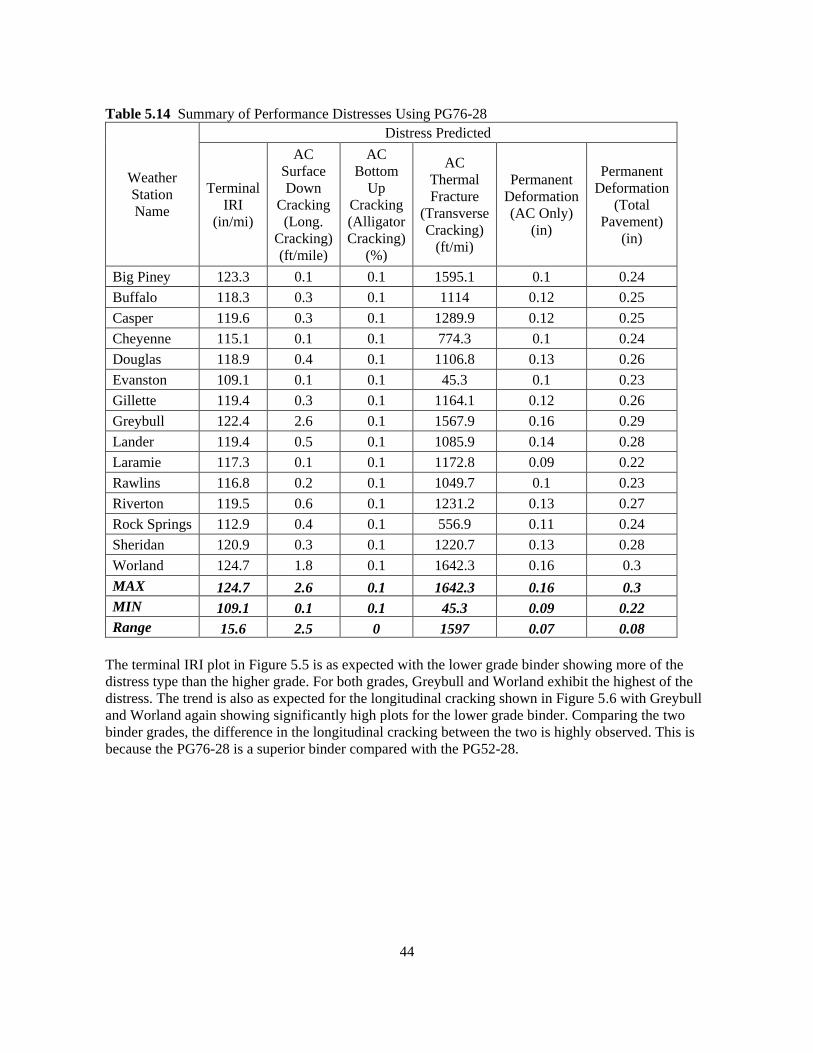
44
Table 5.14 Summary of Performance Distresses Using PG76-28
Weather
Station
Name
Distress Predicted
Terminal
IRI
(in/mi)
AC
Surface
Down
Cracking
(Long.
Cracking)
(ft/mile)
AC
Bottom
Up
Cracking
(Alligator
Cracking)
(%)
AC
Thermal
Fracture
(Transverse
Cracking)
(ft/mi)
Permanent
Deformation
(AC Only)
(in)
Permanent
Deformation
(Total
Pavement)
(in)
Big Piney 123.3 0.1 0.1 1595.1 0.1 0.24
Buffalo 118.3 0.3 0.1 1114 0.12 0.25
Casper 119.6 0.3 0.1 1289.9 0.12 0.25
Cheyenne 115.1 0.1 0.1 774.3 0.1 0.24
Douglas 118.9 0.4 0.1 1106.8 0.13 0.26
Evanston 109.1 0.1 0.1 45.3 0.1 0.23
Gillette 119.4 0.3 0.1 1164.1 0.12 0.26
Greybull 122.4 2.6 0.1 1567.9 0.16 0.29
Lander 119.4 0.5 0.1 1085.9 0.14 0.28
Laramie 117.3 0.1 0.1 1172.8 0.09 0.22
Rawlins 116.8 0.2 0.1 1049.7 0.1 0.23
Riverton 119.5 0.6 0.1 1231.2 0.13 0.27
Rock Springs 112.9 0.4 0.1 556.9 0.11 0.24
Sheridan 120.9 0.3 0.1 1220.7 0.13 0.28
Worland 124.7 1.8 0.1 1642.3 0.16 0.3
MAX 124.7 2.6 0.1 1642.3 0.16 0.3
MIN 109.1 0.1 0.1 45.3 0.09 0.22
Range 15.6 2.5 0 1597 0.07 0.08
The terminal IRI plot in Figure 5.5 is as expected with the lower grade binder showing more of the
distress type than the higher grade. For both grades, Greybull and Worland exhibit the highest of the
distress. The trend is also as expected for the longitudinal cracking shown in Figure 5.6 with Greybull
and Worland again showing significantly high plots for the lower grade binder. Comparing the two
binder grades, the difference in the longitudinal cracking between the two is highly observed. This is
because the PG76-28 is a superior binder compared with the PG52-28.

45
Figure 5.11 International roughness index values for various weather stations.
Figure 5.12 Longitudinal cracking values for various weather stations.
As noted previously, the PG76-28, being a superior grade, tends to contain polymers and so makes the
asphalt mix stiffer. Figure 5.7 shows a plot of the transverse cracking. Due to the stiffness experienced
in the higher grade, it is noted that this type of cracking is higher in the higher grade asphalt. This is
the only pavement distress type where this trend tends to occur. As already noted, Evanston exhibits a
significantly low transverse cracking for both asphalt grade types.
95
100
105
110
115
120
125
130
135
Big
Pin
ey
Bu
ffal
o
Cas
per
Ch
eyen
ne
Do
ugl
as
Evan
sto
n
Gill
ette
Gre
ybu
ll
Lan
der
Lara
mie
Raw
llin
s
Riv
erto
n
Ro
ck S
pri
ngs
Sher
idan
Wo
rlan
d
Term
inal
IRI (
in/m
i)
Weather Stations
PG 52-28
PG 76-28
0102030405060708090
Big
Pin
ey
Bu
ffal
o
Cas
per
Ch
eyen
ne
Do
ugl
as
Evan
sto
n
Gill
ette
Gre
ybu
ll
Lan
der
Lara
mie
Raw
llin
s
Riv
erto
n
Ro
ck S
pri
ngs
Sher
idan
Wo
rlan
d
Lon
gitu
din
al C
rack
ing
(ft/
mi)
Weather Stations
PG 52-28
PG 76-28
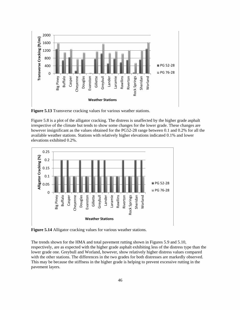
46
Figure 5.13 Transverse cracking values for various weather stations.
Figure 5.8 is a plot of the alligator cracking. The distress is unaffected by the higher grade asphalt
irrespective of the climate but tends to show some changes for the lower grade. These changes are
however insignificant as the values obtained for the PG52-28 range between 0.1 and 0.2% for all the
available weather stations. Stations with relatively higher elevations indicated 0.1% and lower
elevations exhibited 0.2%.
Figure 5.14 Alligator cracking values for various weather stations.
The trends shown for the HMA and total pavement rutting shown in Figures 5.9 and 5.10,
respectively, are as expected with the higher grade asphalt exhibiting less of the distress type than the
lower grade one. Greybull and Worland, however, show relatively higher distress values compared
with the other stations. The differences in the two grades for both distresses are markedly observed.
This may be because the stiffness in the higher grade is helping to prevent excessive rutting in the
pavement layers.
0
400
800
1200
1600
2000
Big
Pin
ey
Bu
ffal
o
Cas
per
Ch
eyen
ne
Do
ugl
as
Evan
sto
n
Gill
ette
Gre
ybu
ll
Lan
der
Lara
mie
Raw
llin
s
Riv
erto
n
Ro
ck S
pri
ngs
Sher
idan
Wo
rlan
d
Tran
sve
rse
Cra
ckin
g (f
t/m
i)
Weather Stations
PG 52-28
PG 76-28
0
0.05
0.1
0.15
0.2
0.25
Big
Pin
ey
Bu
ffal
o
Cas
per
Ch
eyen
ne
Do
ugl
as
Evan
sto
n
Gill
ette
Gre
ybu
ll
Lan
der
Lara
mie
Raw
llin
s
Riv
erto
n
Ro
ck S
pri
ngs
Sher
idan
Wo
rlan
d
Alli
gato
r C
rack
ing
(%)
Weather Stations
PG 52-28
PG 76-28

47
Figure 5.15 HMA rutting values for various weather stations.
Figure 5.16 Total pavement feformation at various weather stations.
5.3.1.3 Virtual Climate Analysis
In areas where there is a deficiency in weather stations, the MEPDG allows for the creation of a virtual
weather station to compensate for such. This is done by interpolation in the software from a group of
known stations that are presented to the engineer, which are deemed to be in close proximity to the
area in question. To create the virtual stations for the above known stations, the actual latitudes,
longitude, and elevations were entered in the MEPDG Version 1.1. The software then presented a set
of six known stations close to the known coordinates. All stations were selected except the one that
showed the actual station data and coordinates for the interpolation as recommended by the MEPDG.
This was classified as the first set of interpolation using all possible MEPDG stations. A second set of
interpolation was carried out where only stations with similar elevations of +/- 500 ft were selected
from the lot and used for the interpolation. The results of both interpolations were analyzed. Table 5.7
is the pavement performance values generated when using virtual stations. Comparing this table with
that of the actual stations shown in Table 5.5, it was noted that all the distresses passed except for
00.05
0.10.15
0.20.25
0.30.35
0.4
Big
Pin
ey
Bu
ffal
o
Cas
per
Ch
eyen
ne
Do
ugl
as
Evan
sto
n
Gill
ette
Gre
ybu
ll
Lan
der
Lara
mie
Raw
llin
s
Riv
erto
n
Ro
ck S
pri
ngs
Sher
idan
Wo
rlan
d
HM
A R
utt
ing
(in
)
Weather Stations
PG 52-28
PG 76-28
0
0.1
0.2
0.3
0.4
0.5
Big
Pin
ey
Bu
ffal
o
Cas
per
Ch
eyen
ne
Do
ugl
as
Evan
sto
n
Gill
ette
Gre
ybu
ll
Lan
der
Lara
mie
Raw
llin
s
Riv
erto
n
Ro
ck S
pri
ngs
Sher
idan
Wo
rlan
d
Tota
l Ru
ttin
g (i
n)
Weather Stations
PG 52-28
PG 76-28

48
transverse cracking and the HMA layer rutting. The number of stations passing in both is similar
except for some that passed for the actual failed, for the virtual, and vice versa. For the HMA rutting,
only the Laramie station passed for both the actual and virtual. Detailed tables of the differences are
included in Appendix D1.
Table 5.15 Pavement Performance –Virtual Station Using All Generated Stations (PG52-28)
Weather
Station
Name
Pavement Distress Predicted
Terminal
IRI
(in/mi)
AC
Surface
Down
Cracking
(Long.
Cracking)
(ft/mile)
AC
Bottom
Up
Cracking
(Alligator
Cracking)
(%)
AC
Thermal
Fracture
(Transverse
Cracking)
(ft/mi)
Permanent
Deformation
(AC Only)
(in)
Permanent
Deformation
(Total
Pavement)
(in)
Big Piney 121.1 4.6 0.1 826.7 0.21 0.36
Buffalo 127.1 5.7 0.1 1496.6 0.22 0.37
Casper 120.6 9.8 0.2 711.3 0.24 0.39
Cheyenne 122.1 1.8 0.1 1117.7 0.18 0.33
Douglas 119.4 7 0.2 649.9 0.23 0.37
Evanston 117.2 2.5 0.1 339.8 0.19 0.34
Gillette 119.1 7.6 0.2 516.8 0.24 0.39
Greybull 124.3 10.8 0.2 1032.1 0.26 0.41
Lander 120.6 15.6 0.2 672.4 0.25 0.4
Laramie 119.3 1 0.1 864 0.16 0.31
Rawlins 120.2 3.5 0.1 826 0.2 0.34
Riverton 121.2 16.3 0.2 584.8 0.27 0.42
Rock Springs 119.5 6.3 0.1 751.6 0.21 0.35
Sheridan 126.2 12.3 0.2 1405.7 0.25 0.4
Worland 119.6 20.5 0.2 401.6 0.28 0.43
MAX 127.1 20.5 0.2 1496.6 0.28 0.43
MIN 117.2 1 0.1 339.8 0.16 0.31
Range 9.9 19.5 0.1 1156.8 0.12 0.12
Table 5.8 shows the annual climate statistics for the virtual weather stations using interpolation of all
the neighboring actual weather stations. No large significant difference was observed between this and
the actual shown in Table 5.1 except for the freezing index where some considerable differences were
noted. Detailed differences are highlighted in Appendix D2.

49
Table 5.16 Climate Statistics Using All Neighboring Stations
Weather
Station
Name
Annual Climate Statistics
Mean
annual air
temperature
(ºF):
Mean
annual
rainfall
(in):
Freezing
index (ºF-
days):
Average
Annual
Number of
Freeze/Thaw
Cycles:
Big Piney 40.9 11.68 1655.95 134
Buffalo 43.06 12.8 1459.03 154
Casper 45.47 10.7 1124.28 131
Cheyenne 43.7 13.32 1233.91 144
Douglas 47.04 11.33 887.24 121
Evanston 40.54 14.13 1676.79 116
Gillette 47.05 12.75 875.94 119
Greybull 47.26 12.46 1006.47 116
Lander 45.02 8.82 1312.4 131
Laramie 41.44 12.94 1398.28 146
Rawlins 41.73 10.94 1486.62 136
Riverton 45.13 11.28 1268.94 138
Rock Springs 41.31 9.25 1609.43 130
Sheridan 48.15 10.9 872.54 111
Worland 47.39 9.87 1080.04 114
MAX 48.15 14.13 1676.79 154
MIN 40.9 8.82 872.54 111
Range 7.25 5.31 804.25 43
Table 5.9 shows the pavement distresses generated using virtual stations generated by interpolation
using neighboring stations that are similar in heights, considering a +/- 500 ft difference. This was also
based on the input screen shown in Appendix A1 but selecting only the stations falling within the
above elevation range. It can also be noted from the table that all the distresses passed except for
transverse cracking and the HMA layer rutting. All the stations failed for the HMA rutting while there
was equal proportion of pass and fail on the transverse cracking.

50
Table 5.17 Pavement Distresses Using Similar Elevations (PG52-28)
Weather
Station
Name
Distress Predicted
Terminal
IRI
(in/mi)
AC
Surface
Down
Cracking
(Long.
Cracking)
(ft/mile)
AC
Bottom
Up
Cracking
(Alligator
Cracking)
(%)
AC
Thermal
Fracture
(Transverse
Cracking)
(ft/mi)
Permanent
Deformation
(AC Only)
(in)
Permanent
Deformation
(Total
Pavement)
(in)
Big Piney 112 5.5 0.1 4.6 0.19 0.33
Buffalo 120.6 7.3 0.2 809.5 0.22 0.37
Casper 120.8 9.4 0.2 735.6 0.24 0.39
Cheyenne 115.5 1.9 0.1 382.1 0.18 0.32
Douglas 120.3 10.3 0.2 724.1 0.24 0.39
Evanston 122.2 9 0.1 1072.4 0.21 0.35
Gillette 119.4 9.6 0.2 530.2 0.24 0.39
Greybull 125.8 24.3 0.2 1024.3 0.29 0.45
Lander 121.2 18.2 0.2 702.7 0.26 0.41
Laramie 118.3 5.8 0.1 775.7 0.19 0.33
Rawlins 112.5 5.3 0.1 99.4 0.19 0.32
Riverton 121.3 19.3 0.2 537.5 0.28 0.43
Rock Springs 120.1 4.9 0.1 986.4 0.18 0.32
Sheridan 126.4 15.6 0.2 1411.4 0.25 0.4
Worland 125.2 32.5 0.2 1059.7 0.29 0.44
MAX 126.4 32.5 0.2 1411.4 0.29 0.45
MIN 112 4.9 0.1 4.6 0.18 0.32
Range 14.4 27.6 0.1 1406.8 0.11 0.13
The climate statistics shown in Table 5.10 have been generated for virtual weather stations
interpolated using similar elevations. A detailed table of differences has been included in Appendix
D2. Similar tables have been produced for the primary and secondary systems highlighting the
significant differences between the data obtained using interpolation based on all the neighboring
stations and that using similar elevations. These are included in Appendix D3 and D4, respectively. A
statistical analysis of the data obtained for the different classes of road has been carried out and are
presented in the subsequent sections. The variability in all the climate variables is minimal except for
the freezing index.

51
Table 5.18 Climate Statistics Using Similar Elevations
Weather
Station Name
Annual Climate Statistics
Mean
annual air
temperature
(ºF):
Mean
annual
rainfall
(in):
Freezing
index (ºF-
days):
Average
Annual
Number of
Freeze/Thaw
Cycles:
Big Piney 43.29 8.03 1238.36 117
Buffalo 45.98 10.98 1028.5 138
Casper 45.36 10.73 1146.45 138
Cheyenne 46.81 12.74 877.67 157
Douglas 47.26 10.56 885.43 128
Evanston 38.84 7.84 2098.26 144
Gillette 47.01 12.2 897.47 123
Greybull 46.13 11.78 1175.34 150
Lander 45.2 8.4 1315.33 121
Laramie 42.2 7.98 1390.44 152
Rawlins 43.92 7.91 1128.66 138
Riverton 45.8 11.36 1187.27 124
Rock Springs 40.77 8.04 1660.99 137
Sheridan 46.61 9.43 1180.55 116
Worland 45.27 8.15 1432.15 133
MAX 47.26 10.56 2098.26 157
MIN 38.84 7.84 897.47 116
Range 8.42 2.72 1200.79 41
5.4 Statistical Analysis
The statistical analysis performed on the output data sort to investigate two things:
1. To determine if there is a difference between the interpolated values and the actual values of
the pavement distresses and annual climate statistics using bootstrapping.
2. Where there are observed differences between interpolated and actual values for the distresses,
use p-values calculations to determine how they correlated with the annual climate factors as
regressor variables. These regressor variables are further defined in the subsequent section.
For the bootstrap confidence intervals, when it was observed that zero was within the interval, it was
concluded that there was no significant difference between interpolated and actual values, and for the
p-values calculations, values less than 0.05 are deemed to be significant or important in predicting the
pavement distress type. Since one of the objectives of this study was to investigate how climate
impacted pavement performance, it was imperative that the annual climate variables be used as the
regressor variables in the regression model for the p-values calculations. This analysis has been
applied to all the different classes of road analyzed in this study. The following section explains the
regression model and terms used in the p-values determination.

52
5.4.1 Regression Models for P-values Calculations
In all cases, the data set considered the actual, interpolated using all generated neighboring stations,
and interpolated using stations that are similar in elevations. Two scenarios were analyzed using the
bootstrap and p-values calculations. Scenario 1 was between the actual and interpolated using all
neighboring stations and Scenario 2 was between actual values and interpolated values using similar
heights. This was applied to the actual differences between interpolated and actual distress values and
also on the percentage change between interpolated and actual.
The general model developed to explain observed differences from the bootstrapping:
Yi = β0 + β1Xi1 + β2Xi2 +β3Xi3 +β4Xi4 + εi
E{Y} = β0 + β1X1 + β2X2 +β3X3 +β4X4 Where:
Y = response variable (pavement performance distresses as defined in section below).
X1, X2, X3, X4 = predictor variables (annual climate variables as defined in section below).
5.4.1.1 Explanation of Regression terms
In this analysis, the response variables (Y) are the pavement distresses: International Roughness Index
(IRI), Transverse Cracking (TC), Alligator Cracking (AC), Longitudinal Cracking (LC), AC Rutting
(ACR), and Total Rutting (TR), the predictor variables (X) are Annual Rainfall (AR), Annual
Temperature (AT), Freezing Index (FI), and Freeze/Thaw Cycle (FT). Based on the general regression
model, a total of 12 regression models were developed:
International Roughness Index (IRI)
ΔIRI1-2 = β0 + β1ΔAR1-2 + β2ΔAT1-2 + β3ΔFI1-2 + β4ΔFT1-2
ΔIRI1-3 = β0 + β1ΔAR1-3 + β2ΔAT1-3 + β3ΔFI1-3 + β4ΔFT1-3
Where:
ΔIRI1-2 = Difference/Percent Change between virtual IRI-2 and actual IRI-1
ΔIRI1-3 = Difference/Percent Change between virtual IRI-3 and actual IRI-1
ΔAR1-2 = Difference/Percent Change between virtual AR-2 and actual AR-1
ΔAR1-3 = Difference/Percent Change between virtual AR-3 and actual AR-1
ΔAT1-2 = Difference/Percent Change between virtual AT-2 and actual AT-1
ΔAT1-3 = Difference/Percent Change between virtual AT-3 and actual AT-1
ΔFI1-2 = Difference/Percent Change between virtual FI-2 and actual FI-1
ΔFI1-3 = Difference/Percent Change between virtual FI-3 and actual FI-1
ΔFT1-2 = Difference/Percent Change between virtual FT-2 and actual FT-1
ΔFT1-3 = Difference/Percent Change between virtual FT-3 and actual FT-1
The designations 1, 2, and 3 represent actual, interpolated based on all stations and interpolated based
on stations with similar elevations, respectively. (See tables in Appendix D).

53
Transverse Cracking (TC)
ΔTC1-2 = β0 + β1ΔAR1-2 + β2ΔAT1-2 + β3ΔFI1-2 + β4ΔFT1-2
ΔTC1-3 = β0 + β1ΔAR1-3 + β2ΔAT1-3 + β3ΔFI1-3 + β4ΔFT1-3
Where:
ΔTC1-2 = Difference/Percent Change virtual TC-2 and actual TC-1
ΔTC1-3 = Difference/Percent Change between virtual TC-3 and actual TC-1
All other terms as defined for the IRI.
Alligator Cracking (AC)
ΔAC1-2 = β0 + β1ΔAR1-2 + β2ΔAT1-2 + β3ΔFI1-2 + β4ΔFT1-2
ΔAC1-3 = β0 + β1ΔAR1-3 + β2ΔAT1-3 + β3ΔFI1-3 + β4ΔFT1-3
Where:
ΔAC1-2 = Difference/Percent Change between virtual AC-2 and actual AC-1
ΔAC1-3 = Difference/Percent Change between virtual AC-3 and actual AC-1
All other terms as defined for the IRI.
Longitudinal Cracking (LC)
ΔLC1-2 = β0 + β1ΔAR1-2 + β2ΔAT1-2 + β3ΔFI1-2 + β4ΔFT1-2
ΔLC1-3 = β0 + β1ΔAR1-3 + β2ΔAT1-3 + β3ΔFI1-3 + β4ΔFT1-3
Where:
ΔLC1-2 = Difference/Percent Change between virtual LC-2 and actual LC-1
ΔLC1-3 = Difference/Percent Change between virtual LC-3 and actual LC-1
All other terms as defined for the IRI.
AC Rutting (ACR)
ΔACR1-2 = β0 + β1ΔAR1-2 + β2ΔAT1-2 + β3ΔFI1-2 + β4ΔFT1-2
ΔACR1-3 = β0 + β1ΔAR1-3 + β2ΔAT1-3 + β3ΔFI1-3 + β4ΔFT1-3
Where:
ΔACR1-2 = Difference/Percent Change between virtual ACR-2 and actual ACR-1
ΔACR1-3 = Difference/Percent Change between virtual ACR-3 and actual ACR-1
All other terms as defined for the IRI.

54
Total Rutting (TR)
ΔTR1-2 = β0 + β1ΔAR1-2 + β2ΔAT1-2 + β3ΔFI1-2 + β4ΔFT1-2
ΔTR1-3 = β0 + β1ΔAR1-3 + β2ΔAT1-3 + β3ΔFI1-3 + β4ΔFT1-3
Where:
ΔTR1-2 = Difference/Percent Change between virtual TR-2 and actual TR-1
ΔTR1-3 = Difference/Percent Change between TR-3 and actual TR-1
All other terms as defined for the IRI.
5.4.1.2 Coefficient of Multiple Determination (R2 and Adjusted R
2)
In analyzing the p-values calculations to determine the level of significance that the climate regressors
have on the response distress variables, the coefficient of multiple determination (R2) and the adjusted
coefficient of multiple determination (Adjusted R2) will also be analyzed for models that show
significance in overall p-values but not for individual regressor p-values. The R2 value for a regression
analysis measures the proportionate reduction of the total variation in the response variable Y
associated with the use of a set of predictor variables X. The value of the R2 is between 0 and 1. The
more the value approaches 1, the better the response Y observations tend to fall directly on the fitted
regression model. However, a large value of R2 does not necessarily imply that the fitted regression
model is a useful one since large X variables will increase the R2 value, hence the use of the adjusted
R2 value, which tends to adjust for the number of predictor X variables (Kutner, Nachtsheim & Neter
2004). The adjusted R2 is always smaller than the R2 as it tends to penalize for an excess number of
predictor variables that do not contribute to the explanatory power of the regression model. For poorly
fitting models, the adjusted R2 value could even become negative.
5.4.1.3 Coefficient of Correlation
The coefficient of correlation is a measure of the association between the response variable Y and the
predictor variables X. It is given by the equation r = +/- (R2)1/2. The value of r is between -1 and 1
(Kutner, Nachtsheim & Neter 2004).
5.4.2 Interstate System
One data set considered the difference between the actual and the two methods of interpolation while
the other used the percentage change between the actual and the interpolated values.
5.4.2.1 Confidence Intervals and P-values Calculations on Differences
Table 5.11 shows the bootstrap confidence intervals and the mean on the actual differences between
virtual distresses and actual distresses. All the terms are as defined previously. Distresses that show no
significant difference between the virtual and the actual are shown in bold and so are statistically
equal. The IRI, AC, and TC all show no significant difference between the actual and virtual values.
All the other distress types, however, show significant differences.

55
Table 5.19 Confidence Intervals for Performance Parameters using Differences
Performance
Distress Mean
95% Confidence Intervals
Lower Bound Upper Bound
ΔIRI1-2 -0.6517 -2.9135 1.7868
ΔIRI1-3 0.3984 -2.0667 2.9602
ΔLC1-2 10.7875 2.3532 22.2867
ΔLC1-3 6.9787 0.0467 16.6338
ΔAC1-2 0.0067 0 0.02
ΔAC1-3 0 0 0
ΔTC1-2 -125.227 -362.04 116.2707
ΔTC1-3 -38.8147 -318.838 249.5932
ΔACR1-2 0.0174 0.0047 0.032
ΔACR1-3 0.0133 0.0007 0.0253
ΔTR1-2 0.0154 0.0027 0.03
ΔTR1-3 0.0133 0.002 0.0253
For the annual climate statistics shown in Table 5.12, it is noted that statistically, there is no significant
difference between actual and virtual stations for all the annual climate parameters irrespective of the
method of interpolation used. It was however observed that the range of confidence interval for the
Freezing Index (FI) based on both methods of interpolation is significantly high as was also observed
for the Transverse Cracking (TC) in Table 5.11 previously.
Table 5.20 Confidence Intervals for Climate Statistics using Differences
Climate
Variable Mean
95% Confidence Intervals
Lower Bound Upper Bound
ΔAR1-2 -1.0537 -2.4248 0.1747
ΔAR1-3 0.7607 -0.6861 1.9921
ΔAT1-2 0.432 -0.6074 1.4147
ΔAT1-3 0.069 -1.0428 0.9927
ΔFI1-2 -11.3319 -191.232 176.0283
ΔFI1-3 12.2038 -178.339 235.6568
ΔFT1-2 -4.6217 -13.1333 4.0667
ΔFT1-3 -9.6439 -20.3333 0.8000
Table 5.13 shows the p-values calculation using the differences between interpolated and actual and
based on the regression models from the previous section. Individual and overall p-values less than
0.05 are shown in bold and indicate importance or significance in predicting the pavement distress. All
the terms in the table are as previously defined. As noted, only the Annual Temperature (ΔAT1-2) is
significant for predicting the Total Rutting (ΔTR1-2). All the others do not show any significance in

56
predicting any of the distresses but the overall p-value for ΔIRI1-2 regression is marginally significant
but it is very significant for the models of ΔIRI1-3 and ΔTC1-3. These also show significant R2 and
adjusted R2. The coefficient of correlation calculation for these two models is also significantly high
implying some degree of correlation among the predictor climate variables. Further statistical analysis
using the correlation matrix method confirms that there is a high degree of multi-collinearity among
the regressor climate variables: freezing index, annual temperature and freeze/thaw cycle. The Annual
Temperature ((ΔAT1-3) and Freezing Index (ΔFI1-3) are significant in predicting the AC Rutting
(ΔACR1-3). Results for interpolation using similar elevation show high significance in p-values than
for that using all the available stations for interpolation.
Table 5.21 P-Values Calculations Using Differences
Performance
Parameter
P-Values Overall
P-values R2
Adjusted
R2 ΔAR1-2 ΔAT1-2 ΔFI1-2 ΔFT1-2
ΔIRI1-2 0.756 0.865 0.489 0.948 0.0445 0.5925 0.4295
ΔTC1-2 0.796 0.437 0.867 0.476 0.0871 0.5257 0.336
ΔAC1-2 0.632 0.682 0.787 0.772 0.6217 0.2137 -0.1008
ΔLC1-2 0.2405 0.1364 0.0842 0.3323 0.0567 0.5699 0.3978
ΔACR1-2 0.7829 0.0729 0.1239 0.0756 0.1955 0.4257 0.196
ΔTR1-2 0.8076 0.044 0.0729 0.0579 0.1344 0.4752 0.2652
Performance
Parameter
P-Values Overall
P-values R2
Adjusted
R2 ΔAR1-3 ΔAT1-3 ΔFI1-3 ΔFT1-3
ΔIRI1-3 0.348 0.827 0.119 0.778 0.0017 0.7975 0.7165
ΔTC1-3 0.945 0.564 0.446 0.624 0.0043 0.7535 0.6549
ΔAC1-3 na na na na na na na
ΔLC1-3 0.7234 0.079 0.0595 0.988 0.0584 0.5669 0.3937
ΔACR1-3 0.3198 0.0169 0.0225 0.3698 0.1262 0.4829 0.2761
ΔTR1-3 0.0664 0.1884 0.2598 0.3561 0.3304 0.344 0.0816
Table 5.14 was derived after further statistical analysis to eliminate the multi-collinearity in the
predictor climate variables. And by using model selection method, further regression analysis was
done to determine the significance in the p-values after the elimination of the multi-collinearity.
Except the alligator cracking which is a load related distress, one or more of the climate variables
showed high significance in predicting the pavement performance parameters. The major ones were
the AT and the FI as noted in Table 5.14 for the interstate system.

57
Table 5.22 Significant Climate Variables for Interstate System
Performance
Parameter
P-Values Overall P-
values R2 Adjusted R2
ΔAR1-2 ΔAT1-2 ΔFI1-2 ΔFT1-2 ΔIRI1-2 - - 0.00096 - 0.00096 0.5806 0.5484
ΔTC1-2 - 0.00489 - - 0.00489 0.4684 0.4275
ΔAC1-2 0.632 0.682 0.787 0.772 0.6217 0.2137 -0.1008
ΔLC1-2 - 0.0374 0.0127 - 0.0200 0.479 0.3921
ΔACR1-2 - 0.0380 0.0464 0.0639 0.09946 0.4211 0.2632
ΔTR1-2 - 0.0306 0.0420 0.0373 0.0625 0.4719 0.3279
Performance
Parameter
P-Values Overall P-
values R2 Adjusted R2
ΔAR1-3 ΔAT1-3 ΔFI1-3 ΔFT1-3 ΔIRI1-3 - - 0.000018 - 0.000018 0.7683 0.7505
ΔTC1-3 - - 0.000039 - 0.000039 0.74 0.72
ΔAC1-3 na na na na na na na
ΔLC1-3 - 0.00283 0.00209 - 0.007239 0.5602 0.4869
ΔACR1-3 0.1392 0.0183 0.0166 - 0.0862 0.4373 0.2839
ΔTR1-3 0.0665 0.0236 0.0193 - 0.1128 0.4063 0.2444
5.4.2.2 Confidence Intervals and P-values Calculations Using Percentage Change
The same analysis was carried out based on the percentage change between the pavement performance
parameters generated by actual weather stations and that by virtual stations to determine the mean and
confidence intervals shown in Table 5.15. The values shown in bold indicate that there is no
significant difference in mean between interpolated and actual values. This indication is, however,
more prominent for values obtained by similar elevations. For the annual climate statistics shown in
Table 5.16, all the climate parameters show no significant difference except for annual rainfall and
freeze/thaw cycle.

58
Table 5.23 Confidence Intervals on Percentage Change
Performance
Parameter Mean
95% Confidence Intervals
Lower Bound Upper Bound
ΔIRI1-2 0.0066 -0.0125 0.0254
ΔIRI1-3 -0.0025 -0.0238 0.0186
ΔLC1-2 -0.363 -0.497 -0.2258
ΔLC1-3 -0.0198 -0.2734 0.2943
ΔAC1-2 -0.0334 -0.1 0
ΔAC1-3 0 0 0
ΔTC1-2 8.5862 0.1123 23.3871
ΔTC1-3 23.9423 -0.1283 71.108
ΔACR1-2 -0.0561 -0.10334 -0.0141
ΔACR1-3 -0.0415 -0.0888 0.0094
ΔTR1-2 -0.0324 -0.0639 -0.0027
ΔTR1-3 -0.0301 -0.0585 0.0002
Table 5.24 Confidence Interval Using Percentage Change
Climate
Statistics Mean
95% Confidence Intervals
Lower Bound Upper Bound
ΔAR1-2 0.166 0.0049 0.3704
ΔAR1-3 -0.0143 -0.1662 0.1973
ΔAT1-2 -0.0083 -0.0304 0.0163
ΔAT1-3 -0.0005 -0.0238 0.0273
ΔFI1-2 0.0637 -0.0847 0.2222
ΔFI1-3 0.0315 -0.0905 0.1561
ΔFT1-2 0.0473 -0.0218 0.1147
ΔFT1-3 0.0926 0.0035 0.1833
Table 5.17 is the p-values table based on using the percentage change of the mean between
interpolated and actual values. The regression model for the ΔIRI1-2 shows a significant overall p-value
with no individual p-value being significant. The model also indicates a large R2 as well as a
significant coefficient of correlation value. The ΔLC1-2 model, as noted, is highly influenced by the
ΔAR1-2, ΔAT1-2, and ΔFT1-2. This is also reflected in the overall p-values and R2 value. The ΔIRI1-3
model indicates that the ΔAR1-3 and ΔFI1-3 are significant in predicting the IRI. The R2 value for this
model is larger than that for the ΔIRI1-2, hence the model using the interpolation based on similar
heights is highly correlated than the model based on the all, interpolation method.

59
Table 5.25 P-Values Calculations Using Percentage Change
Performance
Parameter
P-Values Overall P-
values R2
Adjusted
R2 ΔAR1-2 ΔAT1-2 ΔFI1-2 ΔFT1-2
ΔIRI1-2 0.1918 0.688 0.0535 0.3857 0.0097 0.7077 0.5907
ΔTC1-2 0.893 0.934 0.951 0.59 0.8555 0.1148 -0.2393
ΔAC1-2 0.2751 0.2682 0.0667 0.3833 0.1937 0.427 0.1978
ΔLC1-2 0.0099 0.0287 0.843 0.0112 0.0056 0.7397 0.6356
ΔACR1-2 0.229 0.1201 0.9509 0.0577 0.1152 0.4939 0.2915
ΔTR1-2 0.6012 0.1063 0.5647 0.1323 0.1569 0.4555 0.2376
Performance
Parameter
P-Values Overall P-
values R2
Adjusted
R2 ΔAR1-3 ΔAT1-3 ΔFI1-3 ΔFT1-3
ΔIRI1-3 0.0449 0.7746 0.0122 0.2005 0.0003 0.8609 0.8052
ΔTC1-3 0.995 0.295 0.251 0.275 0.0718 0.5461 0.3646
ΔAC1-3 na na na na na na na
ΔLC1-3 0.6785 0.0491 0.0659 0.8773 0.1022 0.5079 0.3110
ΔACR1-3 0.6633 0.128 0.2034 0.7697 0.4246 0.2979 0.0171
ΔTR1-3 0.2977 0.1213 0.1222 0.8332 0.472 0.2766 -0.0127
5.4.3 Primary System
Table 5.18 shows the confidence intervals calculated for the primary road using the differences
between actual and interpolated stations. All the distresses show no significant difference using at least
one of the two types of interpolation, except the rutting models that show significant difference using
both methods of interpolation. For most of the models generated in Table 5.19, the significance in
their overall p-values is also reflected in their respective high R2 and adjusted R2 values. It can also be
noted that most of the results in Table 5.19 give significantly higher p-values for interpolation using
similar elevations than for the one using all the neighboring stations.

60
Table 5.26 Confidence Intervals on Differences
Performance
Parameter Mean
95% Confidence Intervals
Lower Bound Upper Bound
ΔIRI1-2 -1.6114 -4.1935 0.5467
ΔIRI1-3 0.2738 -3.1335 3.7537
ΔLC1-2 -1.233 -19.735 17.6017
ΔLC1-3 12.2246 -7.8683 30.6683
ΔAC1-2 0.4048 -0.0133 1.2267
ΔAC1-3 0.4435 0.0133 1.2468
ΔTC1-2 -239.473 -508.4488 -30.7918
ΔTC1-3 -54.6112 -426.6638 332.022
ΔACR1-2 0.008 0.002 0.0147
ΔACR1-3 0.006 0.0013 0.0107
ΔTR1-2 0.0086 0.0013 0.016
ΔTR1-3 0.0086 0.002 0.0154
Table 5.27 P-Values Calculations on Differences for Primary System
Performance
Parameter
P-Values Overall P-
values R2
Adjusted
R2 ΔAR1-2 ΔAT1-2 ΔFI1-2 ΔFT1-2
ΔIRI1-2 0.12 0.23 0.114 0.439 0.0721 0.5458 0.3641
ΔTC1-2 0.328 0.516 0.283 0.849 0.3512 0.3333 0.0666
ΔAC1-2 0.533 0.151 0.281 0.128 0.4201 0.3 0.02
ΔLC1-2 0.00006 0.8958 0.4642 0.0064 0.0003 0.8595 0.8033
ΔACR1-2 0.6204 0.0256 0.0312 0.0673 0.0794 0.5357 0.35
ΔTR1-2 0.1791 0.0015 0.008 0.0368 0.0031 0.7711 0.6795
Performance
Parameter P-Values
Overall P-
values R2
Adjusted
R2
ΔAR1-3 ΔAT1-3 ΔFI1-3 ΔFT1-3
ΔIRI1-3 0.453 0.829 0.113 0.375 0.00004 0.9065 0.8691
ΔTC1-3 0.815 0.368 0.428 0.59 0.0002 0.8762 0.8267
ΔAC1-3 0.848 0.607 0.665 0.506 0.9115 0.0864 -0.2791
ΔLC1-3 0.0021 0.6032 0.3071 0.2067 0.0056 0.74 0.636
ΔACR1-3 0.9842 0.0518 0.0851 0.1086 0.1416 0.4687 0.2562
ΔTR1-3 0.0857 0.0097 0.0034 0.4535 0.0084 0.7163 0.6029

61
Table 5.20 was derived by carrying out a model selection method to determine and drop variables as a
result of high multi-collinearity. The table shows the climate variables that are of most significance or
importance in predicting the pavement performance. None of the climate variables are significant in
predicting the alligator cracking because it is a load-related distress. In the primary system also, the
annual temperature and freezing index are the most common climate variables for predicting the
pavement performance.
Table 5.28 Significant Climate Variables for Primary System
Performance
Parameter
P-Values Overall P-
values R2
Adjusted
R2
ΔAR1-2 ΔAT1-2 ΔFI1-2 ΔFT1-2
ΔIRI1-2 - - 0.0218 - 0.02181 0.3429 0.2924
ΔTC1-2 - - 0.0582 - 0.05819 0.2492 0.1914
ΔAC1-2 0.533 0.151 0.281 0.128 0.4201 0.3 0.02
ΔLC1-2 0.00002 - - 0.00104 0.00005 0.8076 0.7755
ΔACR1-2 - 0.0205 0.0199 0.0410 0.03689 0.5236 0.3937
ΔTR1-2 - 0.00255 0.00102 0.02071 0.002105 0.7233 0.6479
Performance
Parameter
P-Values Overall P-
values R2
Adjusted
R2 ΔAR1-3 ΔAT1-3 ΔFI1-3 ΔFT1-3
ΔIRI1-3 0.0295 - 0.000003 - 0.000002 0.8972 0.8801
ΔTC1-3 - 0.000001 - - 0.000001 0.8507 0.8392
ΔAC1-3 0.848 0.607 0.665 0.506 0.9115 0.0864 -0.2791
ΔLC1-3 0.0003 - - - 0.0003 0.6561 0.6296
ΔACR1-3 - 0.01352 0.01542 0.0679 0.0645 0.4687 0.3238
ΔTR1-3 0.02934 0.00904 0.00215 - 0.0033 0.6991 0.617
Table 5.21, on the other hand, is the bootstrap confidence interval based on the percentage change
values. Here also many of the performance distress parameters indicate no significant difference. All
values resulting from interpolation using similar heights show no difference except for the total
pavement rutting that show significant differences for both methods of interpolation. Table 5.22 shows
the results of the p-values calculation using the percentage change values. The overall p-values are
large for ΔLC1-2, ΔIRI1-3, ΔTC1-3, ΔLC1-3, and ΔTR1-3. The R2 and adjusted R2 values also reflect large
values, indicating a significant relation between pavement performance and climate variables.

62
Table 5.29 Confidence Interval Using Percentage Change
Performance
Parameter Mean
95% Confidence Intervals
Lower Bound Upper Bound
ΔIRI1-2 0.0143 -0.004 0.0377
ΔIRI1-3 -0.0006 -0.0291 0.0289
ΔLC1-2 0.0139 -0.0391 0.0741
ΔLC1-3 -0.0281 -0.0816 0.0365
ΔAC1-2 -0.0674 -0.193 0.0162
ΔAC1-3 -0.0951 -0.2179 -0.0136
ΔTC1-2 0.7323 0.0188 2.0498
ΔTC1-3 0.6697 -0.138 2.1466
ΔACR1-2 -0.0464 -0.0852 -0.0039
ΔACR1-3 0.0197 0 -0.0404
ΔTR1-2 -0.0255 -0.0482 -0.0036
ΔTR1-3 -0.0259 -0.0487 -0.0022
Table 5.30 P-Values Calculations Using Percentage Change
Performance
Parameter
P-Values Overall P-
Values R2
Adjusted
R2 ΔAR1-2 ΔAT1-2 ΔFI1-2 ΔFT1-2
ΔIRI1-2 0.652 0.896 0.818 0.454 0.2136 0.413 0.1782
ΔTC1-2 0.891 0.928 0.946 0.589 0.8682 0.1087 -0.2478
ΔAC1-2 0.2661 0.2433 0.3698 0.6077 0.3539 0.332 0.0647
ΔLC1-2 0.000154 0.009136 0.067929 0.077858 0.000016 0.9223 0.8913
ΔACR1-2 0.8234 0.262 0.6072 0.2951 0.3595 0.3292 0.0608
ΔTR1-2 0.8081 0.4571 0.4731 0.6066 0.3139 0.3528 0.09387
Performance
Parameter
P-Values Overall P-
values R2
Adjusted
R2 ΔAR1-3 ΔAT1-3 ΔFI1-3 ΔFT1-3
ΔIRI1-3 0.0694 0.7722 0.0107 0.9431 0.0000084 0.9317 0.9043
ΔTC1-3 0.976 0.361 0.241 0.294 0.04853 0.5846 0.4184
ΔAC1-3 0.0582 0.0761 0.0577 0.7057 0.1877 0.4314 0.2039
ΔLC1-3 0.0283 0.3755 0.8249 0.4897 0.006292 0.7333 0.6267
ΔACR1-3 0.9644 0.0675 0.1851 0.1994 0.0887 0.5237 0.3331
ΔTR1-3 0.1744 0.1342 0.0333 0.6092 0.04899 0.5837 0.4172

63
5.4.4 Secondary System
Table 5.23 shows the mean and confidence interval raw differences for performance distresses
generated using actual weather stations and that use interpolations. Most of the distresses in the table
show statistical equivalence, be it using all the neighboring stations for interpolation or selecting only
stations that have similar elevations.
Table 5.31 Confidence Interval on Differences
Performance
Parameter Mean
95% Confidence Intervals
Lower Bound Upper Bound
ΔIRI1-2 -2.6096 -5.0467 -0.4532
ΔIRI1-3 -0.4464 -3.9668 3.274
ΔLC1-2 -8.4634 -27.2733 1.6133
ΔLC1-3 1.4914 -0.3002 3.2533
ΔAC1-2 -0.0134 -0.04 0
ΔAC1-3 0 0 0
ΔTC1-2 -243.029 -529.758 -6.5047
ΔTC1-3 -86.3897 -493.741 319.2743
ΔACR1-2 0.004 0 0.08
ΔACR1-3 0.0033 0.0013 0.006
ΔTR1-2 -0.00002 -0.0093 0.0073
ΔTR1-3 0.0033 -0.0007 0.0073
Table 5.24 shows the p-values calculated from the regression analysis using the differences generated
for the weather stations and pavement distresses for actual and interpolated weather stations for the
secondary road system. Where overall p-values are observed to be significant but not in the individual
regressor p-values, there exist high multi-collinearity among the regressor variables. Further statistical
analysis was carried out to produce Table 5.25.

64
Table 5.32 P-values on Differences for Secondary System
Regression Analysis
Performance
Parameter
P-Values Overall
P-values R2
Adjusted
R2
ΔAR1-2 ΔAT1-2 ΔFI1-2 ΔFT1-2
ΔIRI1-2 0.1764 0.4126 0.1741 0.6298 0.0688 0.5505 0.3708
ΔTC1-2 0.366 0.814 0.428 0.883 0.3452 0.3364 0.0709
ΔAC1-2 0.847 0.436 0.581 0.383 0.8815 0.1022 -0.257
ΔLC1-2 0.99 0.436 0.568 0.435 0.9186 0.0824 -0.2846
ΔACR1-2 0.3314 0.076 0.161 0.0629 0.1528 0.4589 0.2425
ΔTR1-2 0.85 0.142 0.127 0.186 0.1845 0.4337 0.2072
Performance
Parameter
P-Values Overall
P-values R2
Adjusted
R2 ΔAR1-3 ΔAT1-3 ΔFI1-3 ΔFT1-3
ΔIRI1-3 0.739 0.402 0.323 0.642 0.00008 0.8914 0.848
ΔTC1-3 0.691 0.265 0.544 0.645 0.0001 0.8782 0.8295
ΔAC1-3 na na na na na na na
ΔLC1-3 0.0313 0.4247 0.3009 0.6916 0.1203 0.4887 0.2842
ΔACR1-3 0.3618 0.1604 0.0884 0.1036 0.1235 0.4856 0.2798
ΔTR1-3 0.0246 0.0008 0.0002 0.4336 0.0004 0.8485 0.7878
Table 5.25 shows the variables that have the most effect in predicting the performance parameter.
These variables were determined after multi-collinearity had been determined and removed. The
resulting climate variables were obtained by using the method of model selection. As noted from the
table, annual temperature and freezing index are the two climate parameters that are common in
predicting the performance parameter, except for the alligator cracking. In Table 5.26, the mean and
confidence intervals are based on the percentage change between distresses from actual stations and
that based on interpolated stations. Distresses based on similar elevation interpolation show more
statistical equivalence than those based on interpolation using all the neighboring stations.

65
Table 5.33 Significant Climate Variables for Secondary System
Performance
Parameter
P-Values Overall P-
values R2
Adjusted
R2 ΔAR1-2 ΔAT1-2 ΔFI1-2 ΔFT1-2
ΔIRI1-2 - - 0.0093 - 0.0093 0.4169 0.3721
ΔTC1-2 - - 0.0455 - 0.04547 0.2735 0.2176
ΔAC1-2 0.847 0.436 0.581 0.383 0.8815 0.1022 -0.257
ΔLC1-2 0.99 0.436 0.568 0.435 0.9186 0.0824 -0.2846
ΔACR1-2 - 0.0290 0.0351 0.0837 0.1164 0.4025 0.2396
ΔTR1-2 - - 0.0497 - 0.0497 0.2648 0.2082
Performance
Parameter
P-Values Overall P-
values R2
Adjusted
R2 ΔAR1-3 ΔAT1-3 ΔFI1-3 ΔFT1-3
ΔIRI1-3 - 0.0000003 - - 0.0000003 0.8748 0.8652
ΔTC1-3 - 0.0000008 - - 0.0000008 0.8554 0.8443
ΔAC1-3 na na na na na na na
ΔLC1-3 0.0102 - - - 0.01024 0.4091 0.3637
ΔACR1-3 - - - 0.0620 0.0620 0.2429 0.1846
ΔTR1-3 0.0066 0.0006 0.0001 - 0.0001 0.8384 0.7943
Table 5.34 Confidence Interval on Percentage Change
Performance
Parameter Mean
95% Confidence Intervals
Lower Bound Upper Bound
ΔIRI1-2 0.0226 0.0039 0.0446
ΔIRI1-3 0.0051 -0.0242 0.0343
ΔLC1-2 0.1719 -0.0294 0.5357
ΔLC1-3 -0.0278 -0.0639 0.0107
ΔAC1-2 0.0666 0 0.2
ΔAC1-3 0 0 0
ΔTC1-2 0.9622 0.0188 2.7158
ΔTC1-3 1.0421 -0.1208 3.0841
ΔACR1-2 -0.0521 -0.1156 0.0111
ΔACR1-3 -0.0568 -0.1017 -0.0167
ΔTR1-2 0.0018 -0.0275 0.0392
ΔTR1-3 -0.0124 -0.0286 0.0039

66
Table 5.27 shows p-values calculated from regression analysis using the percentage change generated
for the weather stations and pavement distresses using actual and interpolated weather stations. Only
the AT indicates significance in the prediction of the ACR. There is also a significant overall p-value
with a high R2 value, but the adjusted R2 is marginal. The IRI in the second part of Table 5.27 has a
high overall p-value, but none of the individual explanatory variables show any significance in
predicting the IRI. The corresponding R2 and adjusted R2 values indicate a high degree of goodness of
fit from the variables. As stated in the previous section, this may be due to the high degree of
correlation among the explanatory variables.
Table 5.35 P-values Using Percentage Change
Performance
Parameter
P-Values Overall
P-values R2
Adjusted
R2 ΔAR1-2 ΔAT1-2 ΔFI1-2 ΔFT1-2
ΔIRI1-2 0.857 0.758 0.956 0.436 0.1681 0.4464 0.2249
ΔTC1-2 0.884 0.939 0.947 0.599 0.8662 0.1097 -0.2464
ΔAC1-2 0.538 1.000 0.654 0.459 0.9428 0.0677 -0.3053
ΔLC1-2 0.621 0.917 0.59 0.47 0.96 0.0556 -0.3222
ΔACR1-2 0.6361 0.0056 0.0918 0.2209 0.025 0.6411 0.4976
ΔTR1-2 0.591 0.896 0.996 0.413 0.4573 0.2832 -0.0036
Performance
Parameter
P-Values Overall
P-values R2
Adjusted
R2 ΔAR1-3 ΔAT1-3 ΔFI1-3 ΔFT1-3
ΔIRI1-3 0.383 0.279 0.128 0.85 0.00008 0.8927 0.8498
ΔTC1-3 0.987 0.343 0.241 0.287 0.0517 0.5787 0.4101
ΔAC1-3 na na na na na na na
ΔLC1-3 0.242 0.565 0.829 0.867 0.1656 0.4483 0.2277
ΔACR1-3 0.1687 0.17 0.0731 0.0334 0.149 0.4622 0.247
ΔTR1-3 0.507 0.482 0.149 0.735 0.1243 0.4848 0.2787
5.5 Summary of Statistical Analysis
Using the bootstrapping on the differences, it was observed that for the interstate system the IRI,
alligator cracking and transverse cracking showed no significant difference using any of the
interpolation methods. The other distresses did, however, show some differences even though the
range was minimal. On using the percentage difference, all the distresses showed no significant
change except for the transverse cracking, AC, and total rutting, which showed significant difference
for the interpolation using all the stations. On the climate, no significant difference was noted for the
climate variables for both data sets except for annual rainfall and freeze/thaw in the percentage change
data set. For the p-values calculations based on the differences, only the models for the IRI and the
transverse cracking were deemed to be a good fit having a significant R2 and adjusted R2 values. Using
the percentage data set, the IRI for both methods of interpolation and the longitudinal cracking are
good fits. The IRI using interpolation by similar elevations showed a better fit.

67
For the primary system, using bootstrapping, the IRI, longitudinal cracking, alligator cracking, and
transverse cracking all showed no significant difference using the data set based on the differences. On
using the percentage data set, the AC rutting was included in the above. All these were based on both
methods of interpolation, but for the transverse cracking and AC rutting, these were based on
interpolation based on the similar elevations. P-values calculations based on the differences and
percentage change data showed more correlation in the distress models using similar elevations for the
interpolation. For the secondary system, the bootstrapping for both data sets showed no significant
difference between actual and interpolated distresses, except for the IRI, transverse cracking and the
AC rutting, which showed significant difference based on the interpolation using all the stations. On
examination for the p-values calculations, the distress models based on the interpolation using similar
elevations showed significant correlation with regressors than based on the other interpolation. In all
three classes of road system considered, more of the distress data from interpolation based on similar
weather station elevation showed no significant difference and correlated better with regressors than
for the ones based on interpolation using all the weather stations. The IRI is highly correlated with
regressors than the other distresses irrespective of the dataset based on the interpolation by similar
heights. The correlation is highest in the primary system than for the secondary and interstate. On the
basis of the bootstrapping, the secondary system shows no significant difference for all the distresses
based on the interpolation using similar elevations. It can be concluded that virtual stations based on
similar elevations offer better results than for interpolation based on using all the weather stations.
5.6 Section Summary
In this section, the effect of different binder grade and climate factors on pavement performance was
discussed. The results indicated that the binder grade used and the climate in which the pavement is
constructed do play a significant role its performance. The section also discussed and analyzed the
pavement performance distresses for the different classes of road system in Wyoming using actual
weather data and virtual weather data from interpolation. A statistical analysis using a bootstrap
sampling method was performed to investigate the adequacy of using interpolated weather data to
determine pavement distresses. A regression model was developed using the performance distresses as
response variables and the annual climate variables as regressors from which p-values calculation was
also performed to determine how a specific annual climate variable affected the pavement distresses.
Observations from the bootstrapping and p-values calculations indicated higher significance in using
interpolated values by similar elevations than for using all the available neighboring weather stations.
It should, however, be noted that in running the MEPDG analysis for the different classes of road, the
interstate system kept indicating an on-screen error in the run analysis, which was not observed for the
primary and secondary systems. This was attributed to the asphalt permeable base that was present in
the interstate system but not in the primary and secondary.

68

69
6. CONCLUSIONS AND RECOMMENDATIONS
To satisfy the objectives of this research study, a general study of literature and presentations by
various DOTs on the MEPDG was carried out to determine the level of implementation in the
northwestern states. This literature search identified obstacles to the implementation efforts and how
these could be overcome. Second, MEPDG simulations were conducted using MEPDG software
version 1.1 to analyze how the different climate regions of Wyoming impacted MEPDG pavement
performance. Finally, this study used virtual weather stations created by the MEPDG from
interpolation using two different methods to investigate and statistically analyze its adequacy on
pavement design and performance in the state of Wyoming. The analysis was carried out for interstate,
primary, and secondary road classification systems.
6.1 Conclusions
Having reviewed current literature on the MEPDG, presentations by various states departments of
transportation, and the observations from the climate analysis, the following conclusions can be
drawn:
1. The implementation of the Mechanistic Empirical Pavement Design Guide (MEPDG) will
create more reliable and cost-effective designs and rehabilitation strategies over the traditional
AASHTO guide.
2. The user-oriented computational software program that comes with the MEPDG can predict
pavement conditions over time and thereby help engineers make informed decisions.
3. Adoption of the MEPDG will significantly improve material testing, design procedures, and,
most importantly, data collection.
4. Implementing the MEPDG will require significant amount of time and resources and so
adequate resources should be made available for its implementation.
5. The MEPDG will allow DOTs flexibility to apply and calibrate design procedures to suit local
conditions and thereby achieve more reliable designs.
6. Five additional weather stations with complete weather data were identified for inclusion into
the MEPDG in the State of Wyoming.
7. The variability between actual and virtual climate information was minimal except for the
freezing index where higher variations were observed.
8. The variability in performance parameters at the different locations was minimal except for
transverse cracking. Transverse was therefore identified to be more sensitive to weather data.
9. The transverse cracking model showed failure for all locations except for Evanston and Rock
Springs, which had the two lowest freeze/thaw cycles.
10. The alligator cracking was not affected by the binder grade nor the location. This is because
this is a load-related distress and the load was held consistent in this study.
11. All the pavement performance parameters improved by improving the asphalt grade except for
the transverse cracking. The transverse cracking model needs to be calibrated.

70
12. For all three functional classes of roads, there were higher correlations of performance
parameters when using weather interpolated data based on similar elevations.
13. Performance parameters for the secondary classification were more statistically correlated
than for the primary and interstate.
14. The MEPDG simulation runs on interstate continually indicated errors, which were attributed
to the presence of the asphalt permeable base. Such error was not experienced in the primary
and secondary systems.
6.2 Recommendations
1. Agencies should plan for and monitor future works related to updates and improvements of
the MEPDG and the national and regional levels on a continuous basis.
2. It is important that the MEPDG software be calibrated and validated to suit local conditions,
and so it is imperative that agencies develop and maintain a continuous calibration-validation
database along with input libraries (traffic and material inputs).
3. Construct test sections and periodically monitor them for input parameters and update the
database.
4. The five newly identified weather stations should be added to the MEPDG climate database in
the State of Wyoming.
5. Climate data close to the proposed project site should be used for pavement design and
analysis. Where no weather data is available and interpolations are required, this should be
done based on using climate stations with similar elevations to the project site.

71
REFERENCES
AASHTO. M-E Design: Implementation of a Mechanistic-Empirical Pavement Design. Washington,
DC: AASHTO.
Claros, G. (2007). Updating the Rehabilitation Recommendations in the MEPDG. Transportation
Research Board, Washington DC, 20001
Coree, B. (2005). Implementing the M-E Pavement Design Guide in Iowa. Iowa State University,
Department of Civil, Construction and Environmental Engineering. Ames, IA: Center for
Transportation Reserch and Education.
Coree, B., H. Ceylan & D. Harrington (2005). Implementing the Mechanistic-Empirical Pavement
Design Guide: Implementation Plan. Center for Transportation Research and Education, Iowa
State University.
AASHTO. (2008). Mechanistic-Empirical Pavement Design Guide: A Manual of Practice.
Washington DC: AASHTO.
Coree, B. (2005). Implementing the M-E Pavement Design Guide in Iowa. Iowa State University,
Department of Civil, Construction and Environmental Engineering. Ames, IA: Center for
Transportation Research and Education.
Daniel, J.S. & G.R. Chehab (2007). Use of RAP Mixtures in the Mechanisitc Empirical Pavement
Design Guide. Department of Civil Engineering, University of New Hampshire and
Department of Civil and Environmental Engineering, The Pennsylvania State University.
Durham, NH and University Park, PA: Transportation Research Board 87th Annual Meeting
2008 Washington DC.
Dzotepe, G. & K. Ksaibati (2010). Implementation of the Mechanistic-Empirical Pavement Design
Guide (MEPDG). Laramie: Mountain Plains Consortium.
Haas, R., S. Tighe, G. Dore, G. & D. Hein (2007). Mechanistic-Empirical Pavement Design:
Evolution and Future Challenges. 2007 Annual Transportation Association of Canada
Conference. Saskatoon, Saskatchewan.
Haider, S.W., R.S. Harichandran & M. B. Dwaikat, (2007). Esimating Bimodal Distribution
Parameters And Traffic Levels From Axle Load Spectra. Michigan State University,
Department of Civil and Environmental Engineering. East Lansing, MI: Transportation
Research Board 87th Annual Meeting, 2008, Washington DC.
Hill, K., B. Yohannes & L. Khazanovich (2007). Toward A Unified Mechanistic Approach For
Modeling Tests Of Unbound Materials. University of Minnesota, Department of Civil
Engineering. Minneapolis, MN: Transportation Research Board 87th Annual Meeting, 2008,
Washington DC.

72
Hill, K., B. Yohannes & L. Khazonovich (2007). Toward A Unified Mechanistic Approach For
Modeling Tests Of Unbound Materials. University of Minnesota, Department of Civil
Engineering. Minneapolis, MN: Transportation Research Board 87th Annual Meeting, 2008,
Washington DC.
Kang, M. & T.M. Adams (2007). Local Calibration of the Fatigue Cracking Model in the
Mechanistic-Empirical Pavement Design Guide. University of Wisconsin, Madison,
Department of Civil and Environmental Engineering. Madison, WI: Transportation Research
Board 87th Annual Meeting, 2008, Washington DC.
Katicha, S., G.W. Flintsch, A. Loulizi & L. Wang (2007). Conversion of Testing Frequency to
Loading Time Applied to the Mechanistic-Empirical Pavement Design Guide. Virginia Tech,
Department of Civil and Environmental Engineering. Blacksburg, VA: Transportation
Research Board 87th Annual Meeting, 2008, Washington DC.
Khazanovich, L., S.F. Wojtkiewicz & R. Velasquez (2007). MEPDG-RED: A Framework for
Reliability Analysis With The Mechanistic-Empirical Pavement Design Procedure. University
of Minnesota, Department of Civil Engineering. Minneapolis, MN: Transportation Research
Board 87th Annual Meeting, 2008, Washington DC.
Khazanovich, L., I. Yut, S. Husein, C. Turgeon & T. Burnham (2008). Adaptation of the MEPDG for
the Design of Minnesota Low-Volume Portland Cement Concrete Pavements. Transportation
Research Board 87th Annual Meeting. Washington DC: Transportation Research Board.
Kutner, M.H., C. Nachtsheim & J. Neter (2004). Applied Linear Regression Models (Fourth Edition).
New York: McGraw-Hill/Irvin.
Mehta, Y.A., R.W. Sauber, J. Owad & J. Krause (2007). Lessons Learned During Implementation of
Mechanistic-Empirical Pavement Design Guide. Rowan University, Department of Civil and
Environmental Engineering. Glassboro, NJ: Transportation Research Board 87th Annual
Meeting, 2008, Washington DC.
Muthadi, N.R. & Y.R. Kim (2007). Local Calibration Of The MEPDG For Flexible Pavement Design.
North Carolina State University, Department of Civil, Construction, and Environmental
Engineering. Raleigh, NC: Transportation Research Board 87th Annual Meeting, 2008,
Washington DC.
NCHRP. (2004). Guide for Mechanistic-Empirical Design of New and Rehabilitated Structures.
NCHRP Report 01-37A. Washington DC: Tranportation Research Board.
NCHRP. (2008). NCHRP Report 602: Calibration and Validation of the Enhanced Integrated
Climatic Model for Pavement Design. Washington DC: Transportation Research Board of the
National Academies.
Petry, T.M., Y.P. Han & L. Ge (2007). Determination of Subgrade Soil Field Moisture Conditions
Using Soil Suction. University of Missouri - Rolla, Department of Civil, Architectural and
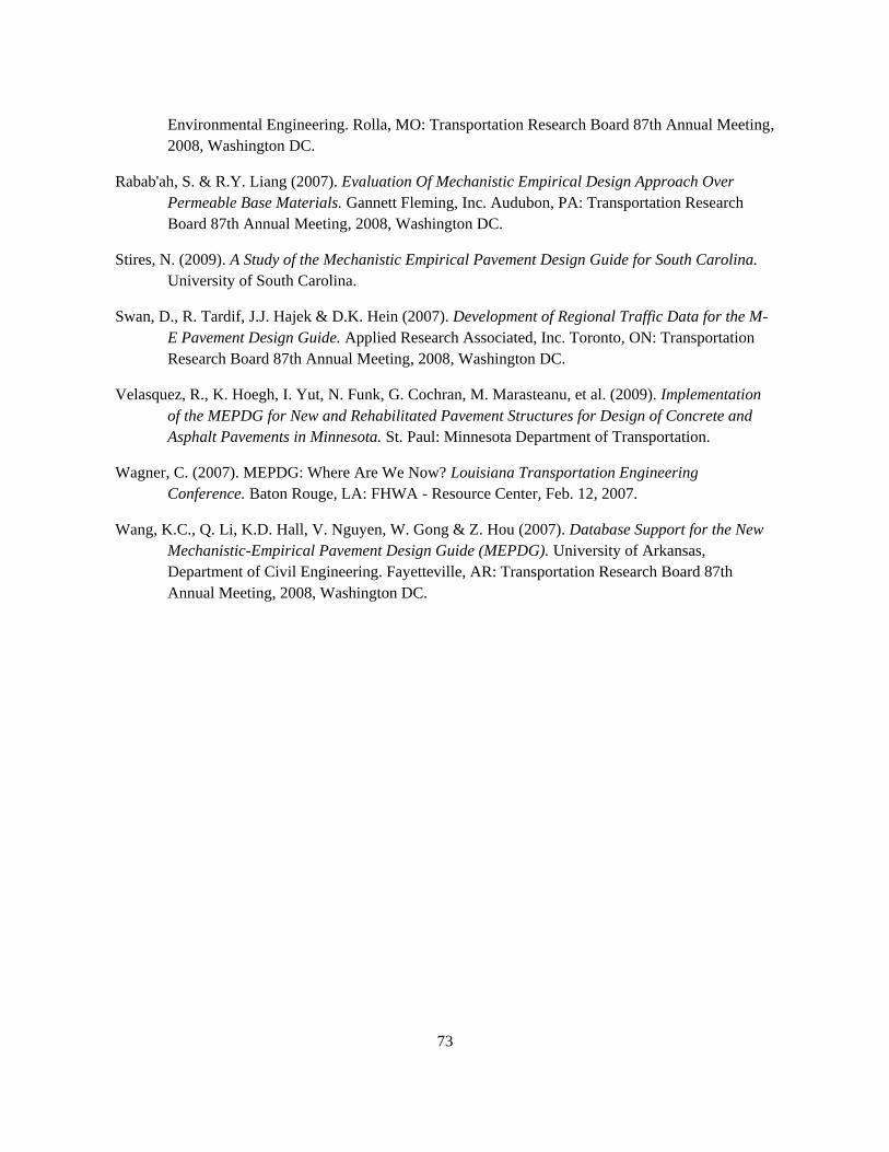
73
Environmental Engineering. Rolla, MO: Transportation Research Board 87th Annual Meeting,
2008, Washington DC.
Rabab'ah, S. & R.Y. Liang (2007). Evaluation Of Mechanistic Empirical Design Approach Over
Permeable Base Materials. Gannett Fleming, Inc. Audubon, PA: Transportation Research
Board 87th Annual Meeting, 2008, Washington DC.
Stires, N. (2009). A Study of the Mechanistic Empirical Pavement Design Guide for South Carolina.
University of South Carolina.
Swan, D., R. Tardif, J.J. Hajek & D.K. Hein (2007). Development of Regional Traffic Data for the M-
E Pavement Design Guide. Applied Research Associated, Inc. Toronto, ON: Transportation
Research Board 87th Annual Meeting, 2008, Washington DC.
Velasquez, R., K. Hoegh, I. Yut, N. Funk, G. Cochran, M. Marasteanu, et al. (2009). Implementation
of the MEPDG for New and Rehabilitated Pavement Structures for Design of Concrete and
Asphalt Pavements in Minnesota. St. Paul: Minnesota Department of Transportation.
Wagner, C. (2007). MEPDG: Where Are We Now? Louisiana Transportation Engineering
Conference. Baton Rouge, LA: FHWA - Resource Center, Feb. 12, 2007.
Wang, K.C., Q. Li, K.D. Hall, V. Nguyen, W. Gong & Z. Hou (2007). Database Support for the New
Mechanistic-Empirical Pavement Design Guide (MEPDG). University of Arkansas,
Department of Civil Engineering. Fayetteville, AR: Transportation Research Board 87th
Annual Meeting, 2008, Washington DC.

74

75
APPENDIX A1: FLEXIBLE PAVEMENT PERFORMANCE PREDICTION EQUATIONS
The prediction equations for flexible pavement distresses have been taken from the Mechanistic-
Empirical Pavement Design Guide, A Manual of Practice, Interim Edition (AASHTO July 2008) and
show the computational steps used in the MEPDG to calculate the distresses. The equations have been
nationally calibrated using field data from the LTPP data and indicate what calibration coefficients
need to be changed to perform local calibration of the distress predictions. The procedure for
computing rutting or plastic vertical deformation, in HMA layers is as shown in the equation. The total
rutting of the pavement structure is summation of the permanent vertical deformation in each layer.
( ) ( ) ( )
Where:
Δp(HMA) = Accumulated permanent or plastic vertical deformation in the HMA layer, in
εp(HMA) = Accumulated permanent or axial strain in the HMA layer/sublayer, in/in
hHMA = Thickness of the HMA layer/sublayer, in.
εr = Resilient or elastic strain calculated by the structural response model at the mid-depth of each
HMA sublayer, in/in.,
n = Number of axle load repetitions
T = Mix or pavement temperature, oF
kz = Depth confinement factor,
k1r, 2r, 3r = Global field calibration parameters (from the NCHRP 1-40D recalibration;
k1r = -3.35412, k2r = 0.4791, k3r = 1.5606)
β1r, 2r, 3r = Local or mixture field calibration constants; for the global calibration,
These constants were all set to 1.0
kz = (C1 + C2D)0.328196D
C1 = - 0.1039(HHMA) 2 + 2.4868HHMA – 17.342
C2 = 0.0172(HHMA) 2 – 1.7330HHMA + 27.428
Where:
D = Depth below surface, in
HHMA = Total HMA thickness, in
( ) { }
{ }
Where:
Δp(soil) = permanent or plastic deformation for the layer/sublayer, in
n = number of axle load applications
ε0 = Intercept determined from laboratory repeated load permanent deformation tests, in/in
εr = Resilient strain imposed in laboratory test to obtain material properties ε0, ε, and ρ, in/in
εv = Average vertical resilient or elastic strain in the layer/sublayer and calculated by the structural
response model, in/in
hsoil = Thickness of the unbound layer/sublayer, in
ks1= Global calibration coefficients; ks1 = 1.673 for granular materials and 1.35 for fine grained
materials
76
εs1= Local calibration constant for the rutting in the unbound layers; the local calibration constant was
set to 1.0 for the global calibration effort.
Logβ = -0.61119 – 0.017638(Wc)
ρ = {
( ( ) )}
C0 = Ln{
} = 0.0075
Wc = Water content, %
Mr = Resilient modulus of the unbound later or sublayer, psi
a1, 9 = Regression constants; a1 = 0.15 and a9 = 20.0
b1, 9 = Regressions constants; b1 = 0.0 and b9 = 0.0
Load Related Cracking
There are two types of load related cracking predicted by the MEPDG; these are the alligator cracking
and longitudinal cracking. It is assumed that alligator cracks are initiated at the bottom of the HMA
layer and propagate to the surface with continued traffic, while the longitudinal cracks initiate at the
surface of the pavement (AASHTO 2008). For both cracking models, the procedure for computing the
allowable number of axle-load applications needed for the incremental damage index is shown using
the following equations:
( )( ) ( ) ( )
Where:
Nf-HMA = Allowable number of axle load applications for a flexible pavement and HMA overlays
εt = Tensile strain at critical locations and calculated by the structural response model in/in
EHMA = Dynamic modulus of the HMA measured in compression, psi
kf1, kf2, kf3 = Global field calibration parameters (from the NCHRP 1-40D recalibration; Kf1= 0.007566,
kf2= -3.9492, kf3= - 1.281).
βf1, f2, f3 = Local or mixture field calibration constants; for the global calibration, these constants were
all set to 1.0.
C = 10M
M = 4.84{
}
Where:
Vbe = Effective asphalt content by volume, %
Va = Percent air voids in the HMA mixture
CH = Thickness term, dependent on type of cracking
For bottom up or alligator cracking
CH =
( )
For top down or longitudinal cracking

77
CH =
( )
Where:
HHMA = Total HMA thickness, in
The area of alligator cracking and length of longitudinal cracking are calculated from the total damage
over time. The relationship used to predict the amount of alligator on the basis of area is as given in
the equation below (AASHTO, 2008).
DI = ∑( ) ∑ (
)
Where:
n = Actual number of axle load applications within a specific time period
j = Axle load interval
m = Axle load type (single, tandem, tridem, quad, or special axle configuration)
l = Truck type using the truck classification groups included in the MEPDG
p = Month
T = Median temperature for the five temperature intervals or quintiles used to subdivide each month, oF.
FCBottom = (
) (
(
) ( ))
Where:
FCBottom = Area of alligator cracking that initiates at the bottom of the HMA layers, % of total lane
area.
DIBottom = Cumulative damage index at the bottom of the HMA layers
C1, 2, 4 = Transfer function regression constants; C4 = 6,000; C1 = 1.00 and C2 = 1.00
C*1 = - 2C*
2
C*2 = - 2.40874 – 39.748(1+HHMA)-2.856
Where:
HHMA = Total HMA thickness, in
FCTop = ( ) (
( ( ))
)
Where:
FCTop = Length of longitudinal cracks that initiate at the top of the HMA layer, ft/mi
DITop = Cumulative damage index near the top of the HMA surface
C1, 2, 4 = Transfer function regression constants; C1 =7.00; C2 = 3.5; C4 = 1,000
Non-Load Related Cracking – Transverse Cracking
The transverse cracking is as a result of the cooling cycle experienced by the pavement. The amount of
this type of crack propagation predicted in the MEPDG uses the Paris law of crack propagation
(AASHTO 2008).
ΔC = A(ΔK)n
Where:
ΔC = Change in the crack depth due to a cooling cycle
ΔK = Change in the stress intensity factor due to a cooling cycle
A, n = Fracture parameters for the HMA mixture
( ( )) Where:

78
[
]
kt = Coefficient determined through global calibration for each input level (Level 1 = 5.0; Level 2 =
1.5; and Level 3 = 3.0)
EHMA – HMA indirect tensile modulus, psi
σm = Mixture tensile strength, psi
m = the m-value derived from the direct tensile creep compliance curve measured in the laboratory
βt = Local or mixture calibration factor
The stress intensity factor K, is given by the equation
K = σtip[0.45 + 1.99(C0)0.56]
Where:
σtip = Far-field stress from pavement response model at the depth of crack tip, psi
C0 = Current crack length, ft
The degree of transverse cracking is predicted by
[
(
)]
Where;
TC = Observed amount of thermal cracking, ft/mi
βt1 = Regression coefficient determined through global calibration (400)
N[z] = Standard normal distribution evaluated at [z]
σd = Standard deviation of the log of the depth of cracks in the pavement (0.769), in
Cd = Crack depth, in
HHMA = Thickness of HMA layers, in
IRI Computation
The equation embedded in the MEPDG for the prediction of IRI is as given below. The equation
applies to new HMA pavements and HMA overlays of Flexible pavements.
IRI = IRI0 + 0.0150(SF) + 0.400(FCTotal) + 0.0080(TC) + 40.0(RD)
Where:
IRI0 = Initial IRI after construction, in/mi
SF = Site factor (equation given below)
FCTotal = Area of fatigue cracking (combined alligator, longitudinal and reflection cracking in the
wheel path), percent of total lane area. All load related cracks are combined on an area basis
– length of cracks is multiplied by 1ft to convert length into an area basis.
TC = Length of transverse cracking (including the reflection of transverse cracks in existing HMA
pavements), ft/mi
RD = Average rut depth, in.
SF = Age [0.02003(PI + 1) + 0.007947(Precip + 1) + 0.000636(FI + 1)]
Where:
Age = Pavement age, yr
PI = Percent plasticity index of the soil
FI = Average annual freezing index, oF days
Precip = Average annual precipitation or rainfall, in

79
APPENDIX A2: MEPDG DATA INPUT SCREENS

80
Figure A2.1 Main MEPDG Data Input Screen

81
Figure A2.2 General Information Screen (I-80)
Figure A2.3 Analysis Parameter Screen (I-80)

82
Figure A2.4 AADTT Calculator
Figure A2.5 Traffic Input Screen (I-80)
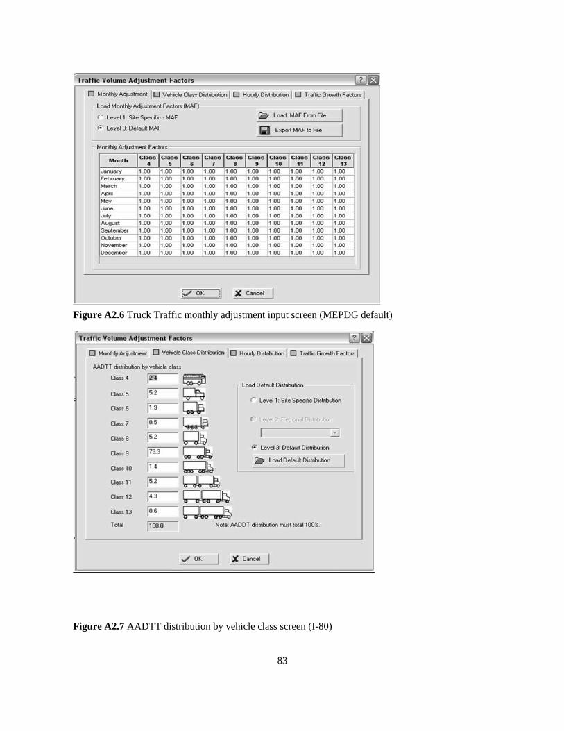
83
Figure A2.6 Truck Traffic monthly adjustment input screen (MEPDG default)
Figure A2.7 AADTT distribution by vehicle class screen (I-80)
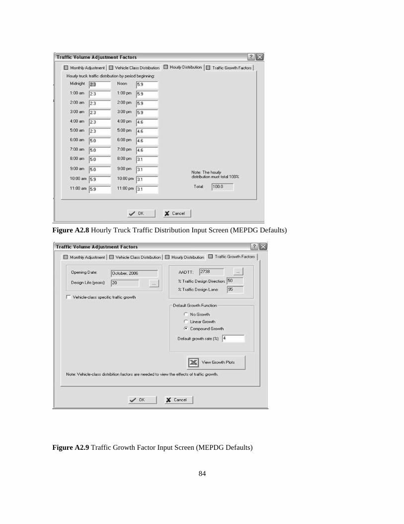
84
Figure A2.8 Hourly Truck Traffic Distribution Input Screen (MEPDG Defaults)
Figure A2.9 Traffic Growth Factor Input Screen (MEPDG Defaults)

85
Figure A2.10 Axle Load Distribution Factors Input Screen (MEPDG Default)
Figure A2.11 Number of Axles per Truck Input Screen (MEPDG Default)

86
Figure A2.12 Axle Configuration Input Screen (MEPDG Defaults)
Figure A2.13 Truck Wheelbase Input Screen (MEPDG Defaults)

87
Figure A2.14 Pavement Structure Input Screen (I-80)
Figure A2.15 Asphalt Mix Input Screen (I-80)

88
Figure A2.16 Asphalt Binder Selection Input Screen (I-80)
Figure A2.17 Asphalt General Properties Input Screen (I-80)

89
Figure A2.18 Strength Properties Input Screen for Unbound Materials

90
Figure A2.19 EICM Inputs for Unbound Materials
Figure A2.20 Input Screen for Thermal Cracking (MEPDG Default)

91
APPENDIX B1: PAVEMENT DATABASE SURFACE/BASE TYPE DESIGNATIONS
Pavement Database Surface/Base Type Designations
The following designations were defined for use in the pavement management system.
Pavements:
G1: Standard PM Pavement with chip seal.
G2: Standard PM Pavement with plant mix wearing course.
G3: PM overlay of PCC pavement, no crack and seat.
G4: PM overlay of crack & seated PCC pavement.
G5: Plain jointed PCC pavement with PM inlay in driving lane.
G6: Standard PM Pavement with microsurfacing (DL or Full-width).
J1: Plain jointed full width PCC pavement.
J2: Dowel jointed full width PCC pavement.
J3: Plain jointed PCC pavement with PM pavement shoulders.
J4: Dowel jointed PCC pavement with PM pavement shoulders.
J5: PM pavement with PCC pavement inlay in driving lane.
J6: Dowel retrofitted Plain Jointed PCC pavement with PM pavement shoulders.
J7: Dowel retrofitted Plain Jointed full width PCC pavement.
K1: Plain jointed PCC pavement overlay (whitetop) over PM pavement
K2: Dowel jointed PCC pavement overlay (whitetop) over PM pavement
Bases:
AG: Aggregate base or rubblized cement treated base
PM: Plant mix treated base
CT: Cement treated base
AP: Asphalt treated permeable base
UP: Untreated permeable base
PC: Cracked and seated PCC pavement base
LT: Lime Stabilized Subgrade

92

93
APPENDIX B2: EXTRACT FROM PRIMARY ROAD PMS

94
SYS
TEM
RO
UTE
BEG_
MP
END_
MP
PAV
E_TY
PE
LAST_
REHA
B
AAD
T
ESA
L
PAVE
_DEP
TH
BASE
_TYP
E
BASE_
DEPT
H
P 10 0 2.37 G2 1987 1120 303 4 AG 6
P 10 1.122 11.59 G2 1989 1827 195 4 AG 6
P 10 84.93 85.59 G2 1988 3750 311 4 AG 6
P 10 85.59 87.16 G2 1987 4193 412 5 AG 6
P 10 118.3 120.9 G2 1999 1985 392 5 AG 6
P 10 120.9 127.2 G2 2001 1900 392 4 AG 6
P 10 127.2 132 G2 1998 1925 392 4 PM 7
P 10 132 136 G2 2002 1925 392 4 PM 6
P 10 136 139.3 G2 2000 1973 392 5 PM 6
P 10 139.3 142.5 G2 1986 2760 397 2 AG 5
P 10 142.5 146.8 G2 1982 3130 427 4 AG 4
P 10 146.8 148 G2 1977 3630 468 2 PM 6
P 10 148 151 G2 1998 4902 488 4 AG 9
P 10 151 154.3 G2 1989 9993 666 5 AG 4
P 10 155.1 158.8 G2 1973 4330 370 4 AG 4
P 13 0 1.147 G2 1983 7330 378 7 AG 6
P 13 1.618 2.867 G2 1995 3530 625 4 PM 7
P 13 2.867 4.71 G2 1995 1350 629 4 AG 11
P 13 111.3 115.3 G2 1987 995 191 6 AG 4
P 14 57.04 62.97 G2 1993 737 232 4 AG 17
P 16 96.96 99.02 G2 1990 2948 218 6 AG 4
P 20 47.22 54.37 G2 1990 360 150 6 AG 4
P 20 80.02 81.11 G2 1997 4513 305 4 PM 9
P 20 81.11 82.32 G2 2002 3170 337 7 AG 7
P 20 90.87 104.1 G2 1994 4381 465 4 PM 5
P 20 104.1 105.1 G2 2007 7418 459 10 AG 5
P 20 109.7 119.1 G2 1986 2018 540 7 AG 4
P 21 0.768 2.286 G2 1997 3003 442 4 AG 8
P 21 38.6 44.31 G2 2003 905 571 6 AG 4
P 21 79.6 88 G2 1989 1255 637 5 AG 8
P 21 88 94.08 G2 1990 1485 749 5 AG 4
P 21 94.08 98 G2 2000 1740 687 8 AG 4
P 21 98 101.1 G2 2000 1818 798 7 AG 4
P 21 101.1 106 G2 2000 2183 769 6 AG 4
P 21 106 107.9 G2 2000 2058 891 6 CT 4
P 21 107.9 111.7 G2 1995 4106 600 3 CT 4
P 21 111.7 113.2 G2 1992 11038 805 7 CT 4
P 21 114.8 115.3 G2 2005 6460 237 3 AG 6

95
SYS
TEM
RO
UTE
BEG_
MP
END_
MP
PAV
E_TY
PE
LAST_
REHA
B
AAD
T
ESA
L
PAVE
_DEP
TH
BASE
_TYP
E
BASE_
DEPT
H
P 21 115.4 115.7 G2 1981 6607 245 5 AG 10
P 21 116.5 117.2 G2 1969 8927 637 3 AG 4
P 23 326.9 327.2 G2 1982 2730 143 4 AG 4
P 23 327.2 327.4 G2 1990 3670 156 6 AG 12
P 23 327.4 328.2 G2 1982 7750 271 6 AG 12
P 23 328.2 400.1 G2 1975 6675 278 3 AG 9
P 23 400.1 400.9 G2 1965 4895 660 3 AG 4
P 23 402.3 411.9 G2 1995 2380 545 6 PM 6
P 23 419.3 421.6 G2 1985 1585 621 4 CT 6
P 23 421.6 424.5 G2 1978 1585 621 7 PM 7
P 23 424.5 425.4 G2 1995 2069 660 4 PM 7
P 25 92.02 93.11 G2 1994 4478 393 3 AG 5
P 25 93.63 95.01 G2 1976 4775 472 4 AG 6
P 25 95.01 103.3 G2 1997 2353 569 4 PM 5
P 25 149 149.2 G2 2002 1700 186 6 AG 9
P 25 149.3 149.7 G2 2002 2748 407 6 AG 9
P 25 149.8 149.9 G2 2002 2510 377 6 AG 9
P 25 149.9 150.2 G2 1988 2200 375 5 AG 6
P 25 184.9 190.3 G2 1999 825 329 5 CT 9
P 25 190.3 192 G2 1999 689 285 5 CT 11
P 25 192 195.8 G2 1999 554 214 9 CT 11
P 25 195.8 202.6 G2 1995 413 123 5 CT 10
P 25 222.2 225.9 G2 1996 511 151 4 AG 18
P 25 225.9 229.3 G2 1996 708 159 4 AG 18
P 26 0 0.295 G2 1963 5865 195 4 AG 4
P 26 0.295 0.82 G2 1988 6099 218 5 AG 6
P 26 0.82 1.263 G2 1977 6006 181 6 AG 8
P 26 1.377 2.598 G2 1988 2905 180 5 AG 15
P 27 23.22 38.42 G2 2000 1157 424 7 AG 4
P 27 48.63 56.26 G2 1991 2712 379 5 PM 5
P 29 0.685 2.253 G2 2006 5455 360 7 AG 10
P 29 13.05 19.29 G2 2004 2407 385 4 AG 14
P 29 19.29 23.35 G2 2004 3130 275 5 CT 15
P 29 24.18 25.02 G2 2002 1710 190 6 AG 4
P 30 130.7 133.7 G2 1999 5712 186 9 AG 8
P 31 0 10 G2 1997 590 59 4 PM 8
P 31 27.47 36.41 G2 1975 698 69 2 AG 4
P 31 45.89 51.08 G2 2002 3093 202 6 AG 4

96
SYS
TEM
RO
UTE
BEG_
MP
END_
MP
PAV
E_TY
PE
LAST_
REHA
B
AAD
T
ESA
L
PAVE
_DEP
TH
BASE
_TYP
E
BASE_
DEPT
H
P 31 51.08 51.78 G2 1994 4525 348 2 AG 4
P 31 52.96 54.8 G2 1994 3283 289 3 AG 4
P 33 0 0.674 G2 2003 1425 194 3 AG 5
P 33 38.18 43.12 G2 1994 550 170 5 CT 10
P 33 43.12 51.31 G2 1996 726 294 5 CT 9
P 33 72.91 81.21 G2 1991 1073 264 4 PM 8
P 34 0 2.89 G2 1990 4593 680 3 AG 4
P 34 0 1.1 G2 1999 4920 103 3 AG 4
P 34 3.874 10.37 G2 1990 5389 474 6 AG 8
P 34 10.36 21.24 G2 2002 1535 509 7 AG 17
P 34 164.1 164.6 G2 2006 1715 286 5 AG 14
P 34 164.7 165.4 G2 2000 2245 322 7 AG 6
P 34 165.8 166 G2 1985 4095 405 4 AG 4
P 34 186.3 197.7 G2 1991 1932 420 6 PM 4
P 34 202.6 203.6 G2 2005 2740 258 5 AG 12
P 34 203.6 205 G2 2007 3233 331 5 AG 8
P 34 205 205.3 G2 1962 2055 374 3 AG 4
P 36 80.09 87.16 G2 2003 620 87 5 AG 6
P 36 87.16 88.39 G2 2003 753 73 5 AG 6
P 36 90.83 91.96 G2 1990 3040 112 4 AG 4
P 36 100 100.7 G2 2003 3420 441 8 AG 4
P 37 20.36 20.55 G2 1992 310 48 4 AG 2
P 37 20.55 26.41 G2 1992 497 61 6 AG 6
P 37 61.6 66.3 G2 1999 453 56 4 AG 6
P 37 83.45 88.91 G2 2000 1235 100 3 PM 5
P 42 10.95 21.04 G2 1999 820 228 6 AG 9
P 43 8.662 18.21 G2 1997 1150 359 9 CT 11
P 43 107 111.2 G2 2000 8245 505 6 CT 10
P 43 111.2 112 G2 1994 19060 794 4 CT 8
P 43 113.1 114.9 G2 1979 7770 657 6 AG 6
P 43 114.9 115.2 G2 1981 8299 793 3 PM 10
P 43 115.3 115.4 G2 1981 3750 705 3 PM 10
P 43 115.4 115.4 G2 1984 3850 711 3 PM 10
P 43 115.5 118.8 G2 1981 1268 184 3 PM 10
P 44 0 0.252 G2 1963 1100 192 2 AG 4
P 49 0 0.381 G2 1988 1935 105 5 AG 6
P 49 1.084 1.764 G2 2004 1700 74 7 AG 9
P 51 4.324 4.646 G2 1996 4900 498 4 PM 6

97
SYS
TEM
RO
UTE
BEG_
MP
END_
MP
PAV
E_TY
PE
LAST_
REHA
B
AAD
T
ESA
L
PAVE
_DEP
TH
BASE
_TYP
E
BASE_
DEPT
H
P 51 4.646 4.768 G2 1975 5760 311 3 AG 6
P 53 102.8 103.8 G2 1986 10035 464 5 PM 11
P 53 104.8 104.8 G2 1985 7316 324 2 CT 4
P 54 212 212 G2 1994 3885 319 6 AG 7
P 55 328.5 330.4 G2 1988 9085 169 5 AG 4
P 55 330.4 330.7 G2 1988 9544 224 5 AG 4
P 55 330.7 331 G2 1973 9402 219 5 AG 4
P 55 331 331.2 G2 1988 8572 214 5 AG 4
P 55 331.2 332.2 G2 1992 3073 224 4 AG 4
P 56 362.9 363.2 G2 1985 8310 229 8 AG 4
P 56 363.6 364.3 G2 1985 7888 205 5 AG 4
P 56 364.3 365.2 G2 1978 4100 152 3 PM 11
P 56 365.2 365.8 G2 1977 3830 174 3 PM 9
P 56 365.8 371.1 G2 1982 2233 116 5 AG 4
P 57 78.93 79 G2 1976 2570 150 3 AG 8
P 57 79.42 80.89 G2 1996 1545 100 4 AG 8
P 58 135.8 136.5 G2 1990 2565 208 7 AG 6
P 58 136.5 138 G2 1967 4025 236 3 AG 4
P 58 138 138.8 G2 1980 5403 228 4 AG 4
P 58 138.8 139.2 G2 1986 3550 104 3 PM 4
P 58 139.2 140 G2 1982 3895 138 4 AG 4
P 59 298.6 300.4 G2 1991 2829 146 3 PM 5
P 60 20.92 21.14 G2 1998 4925 350 4 CT 6
P 60 21.14 21.65 G2 1998 3940 190 4 CT 6
P 60 23.48 23.99 G2 1998 7289 274 3 PM 2
P 60 23.91 24.34 G2 1998 10070 213 3 PM 9
P 60 24.34 25.16 G2 1998 11182 324 4 PM 9
P 61 0.022 0.279 G2 1987 4750 181 4 AG 4
P 62 124.5 125.5 G2 1979 7589 336 6 AG 6
P 62 126.2 126.4 G2 2001 4325 392 5 CT 6
P 62 126.4 127.2 G2 2001 5569 255 8 CT 8
P 62 127.2 127.2 G2 2001 4423 317 6 CT 6
P 62 127.2 127.6 G2 2001 7589 336 4 CT 6

98
0
2
4
6
8
10
12
14
16
18
20
AG
PM AG
AG
PM AG CT
AG
PM AG
AG
AG
AG
AG
AG
AG
AG CT
PM AG
AG
PM AG
PM CT
BASE TYPE
Base Depth(in)
PavementDepth (in)

99
APPENDIX B3: EXTRACT FROM SECONDARY ROAD PMS
SYST
EM
ROU
TE
BEG
_MP
END_
MP
PAVE
_TYP
E
LAST_
REHA
B
AAD
T
ESA
L
PAVE
_DEPT
H
BASE
_TYP
E
BASE_
DEPT
H
S 107 3.92 10.4 G2 2004 1340 74 3 AG 12
S 109 28.5 30.6 G2 1997 274 30 4 AG 6
S 109 30.6 35.8 G2 1997 240 24 4 AG 6
S 109 35.8 45.1 G2 1995 335 40 4 AG 9
S 109 45.1 52.2 G2 1994 423 46 4 AG 6
S 302 89.3 99.3 G2 2002 880 114 2 AG 12
S 504 0 0.18 G2 2004 640 42 8 AG 8
S 504 0.18 1.38 G2 2004 746 24 8 AG 8
S 504 1.38 2.13 G2 2004 1033 61 10 AG 6
S 505 165 165 G2 1963 1419 83 3 AG 6
S 505 165 166 G2 2004 1668 82 6 AG 6
S 505 166 172 G2 1996 1150 89 5 AG 12
S 505 172 176 G2 1997 1260 89 5 AG 12
S 505 176 179 G2 1998 1260 89 7 AG 7
S 505 179 181 G2 1998 1260 89 7 AG 6
S 505 181 184 G2 1998 1450 108 7 AG 6
S 1501 1.66 2.74 G2 1979 1240 78 2 AG 6
S 1501 2.77 6.52 G2 1995 835 54 2 AG 6
S 1501 6.52 9.44 G2 1995 986 60 2 AG 6
S 1604 0.09 1.64 G2 1999 342 18 4 AG 8
S 1703 0 3.14 G2 2002 2190 78 5 AG 6
S 2000 0 3.67 G2 1984 8305 346 5 PM 7
S 2000 3.85 4.01 G2 1975 7095 264 6 AG 3
S 2000 4.01 6.58 G2 1984 3852 246 5 AG 6
S 2000 6.58 13.7 G2 2005 2100 83 2 AG 6
S 2000 13.7 17.5 G2 2005 1972 81 4 AG 4
S 2001 0 0.14 G2 1975 5335 226 4 AG 3
S 2001 0.14 6.63 G2 1971 4205 183 3 AG 4
S 2106 34.7 35.5 G2 2006 1015 66 8 AG 6
S 2106 35.4 42.3 G2 2006 1715 82 8 AG 6
S 2106 42.3 43.4 G2 1997 2053 76 3 AG 6
S 2303 27.3 28.1 G2 1995 883 111 4 AG 10

100
APPENDIX B4: EXTRACTS FROM I-80 PMS

101
SYST
EM
RO
UT
E
BEG
_MP
END_
MP
PAVE
_TYPE
LAST_
REHA
B
AAD
T
ESA
L
PAVE_
DEPT
H
BASE
_TYP
E
BASE_
DEPT
H
I 80 28.1 39 G2 1997 6453 5100 5 CT 6
I 80 39 28.1 G2 1997 6453 5100 5 CT 6
I 80 39 44 G2 1998 5855 4706 6 PM 6
I 80 44 39 G2 1998 5855 4706 6 PM 6
I 80 44 49 G2 1997 5800 4736 6 PM 6
I 80 49 44 G2 1997 5800 4736 6 PM 6
I 80 49 53 G2 2000 5800 4745 9 CT 6
I 80 53 49 G2 2000 5800 4745 9 CT 6
I 80 53 57 G2 2000 5800 4753 8 CT 6
I 80 57 53 G2 2000 5800 4753 8 CT 6
I 80 57 65.4 G2 2003 5758 4740 17 PM 6
I 80 65.4 57 G2 2003 5758 4740 16 PM 6
I 80 65.4 76 G2 1995 6545 5906 4 PM 6
I 80 76 65.4 G2 1995 6545 5906 4 PM 6
I 80 76 83 G2 1996 6695 5919 9 CT 6
I 80 83 76 G2 1996 6695 5919 9 CT 6
I 80 143 148.5 G2 1998 6090 5633 6 PM 6
I 80 149 143 G2 1998 6090 5633 6 PM 6
I 80 149 153.8 G2 1998 6085 5633 6 PM 6
I 80 154 148.5 G2 1998 6085 5633 6 PM 6
I 80 216 221.2 G2 2000 6455 6071 10 CT 6
I 80 221 216.2 G2 2000 6455 6071 10 CT 6
I 80 221 227.5 G2 1997 6355 6062 8 CT 6
I 80 228 221.2 G2 1997 6355 6062 8 CT 6
I 80 228 233.7 G2 2001 6215 5907 6 CT 6
I 80 234 227.5 G2 2001 6215 5907 6 CT 6
I 80 246 252 G2 1999 5975 5718 8 PM 6
I 80 252 245.9 G2 1999 5975 5718 8 PM 6
I 80 252 258.6 G2 1999 5975 5718 10 PM 6
I 80 259 252 G2 1999 5975 5718 10 PM 6
I 80 276 280.7 G2 2001 5490 5476 6 PM 6
I 80 281 275.6 G2 2001 5490 5476 6 PM 6
I 80 281 285 G2 2001 5430 5391 6 PM 6
I 80 285 280.7 G2 2001 5430 5391 6 PM 6
I 80 290 295 G2 2004 5430 5391 8 CT 6
I 80 295 289.9 G2 2004 5430 5391 8 CT 6
I 80 295 299.5 G2 2004 5430 5391 8 CT 6
I 80 300 295 G2 2004 5430 5391 8 CT 6

102
SYST
EM
RO
UT
E
BEG
_MP
END_
MP
PAVE
_TYPE
LAST_
REHA
B
AAD
T
ESA
L
PAVE_
DEPT
H
BASE
_TYP
E
BASE_
DEPT
H
I 80 300 310.5 G2 1991 5535 5191 11 CT 6
I 80 311 299.5 G2 1991 5535 5191 11 CT 6
I 80 324 329.6 G2 2005 6245 5233 7 CT 6
I 80 330 324 G2 2005 6245 5233 7 CT 6
I 80 330 336.6 G2 2006 6245 5233 7 CT 6
I 80 337 329.6 G2 2006 6245 5233 7 CT 6
I 80 337 348.5 G2 2004 6382 5278 14 CT 6
I 80 349 336.6 G2 2004 6382 5278 14 CT 6
I 80 28.1 39 G2 1997 6453 5100 5 CT 6
I 80 39 28.1 G2 1997 6453 5100 5 CT 6
I 80 39 44 G2 1998 5855 4706 6 PM 6
I 80 44 39 G2 1998 5855 4706 6 PM 6
I 80 44 49 G2 1997 5800 4736 6 PM 6
I 80 49 44 G2 1997 5800 4736 6 PM 6
I 80 49 53 G2 2000 5800 4745 9 CT 6
I 80 53 49 G2 2000 5800 4745 9 CT 6
I 80 53 57 G2 2000 5800 4753 8 CT 6
I 80 57 53 G2 2000 5800 4753 8 CT 6
I 80 57 65.4 G2 2003 5758 4740 17 PM 6
I 80 65.4 57 G2 2003 5758 4740 16 PM 6
I 80 65.4 76 G2 1995 6545 5906 4 PM 6
I 80 76 65.4 G2 1995 6545 5906 4 PM 6
I 80 76 83 G2 1996 6695 5919 9 CT 6
I 80 83 76 G2 1996 6695 5919 9 CT 6
I 80 108 120.3 G2 2003 6515 5747 9 CT 6
I 80 120 107.6 G2 2003 6515 5747 9 CT 6
I 80 120 130 G2 1996 6490 5550 8 CT 6
I 80 130 120.3 G2 2001 6490 5550 8 CT 6
I 80 138 130 G2 2001 6190 5208 11 CT 6
I 80 138 143 G2 1994 6040 5198 19 PM 6
I 80 143 138 G2 1994 6040 5198 19 PM 6
I 80 143 148.5 G2 1998 6090 5633 6 PM 6
I 80 149 143 G2 1998 6090 5633 6 PM 6
I 80 149 153.8 G2 1998 6085 5633 6 PM 6
I 80 154 148.5 G2 1998 6085 5633 6 PM 6
I 80 216 221.2 G2 2000 6455 6071 10 CT 6
I 80 221 216.2 G2 2000 6455 6071 10 CT 6
I 80 221 227.5 G2 1997 6355 6062 8 CT 6
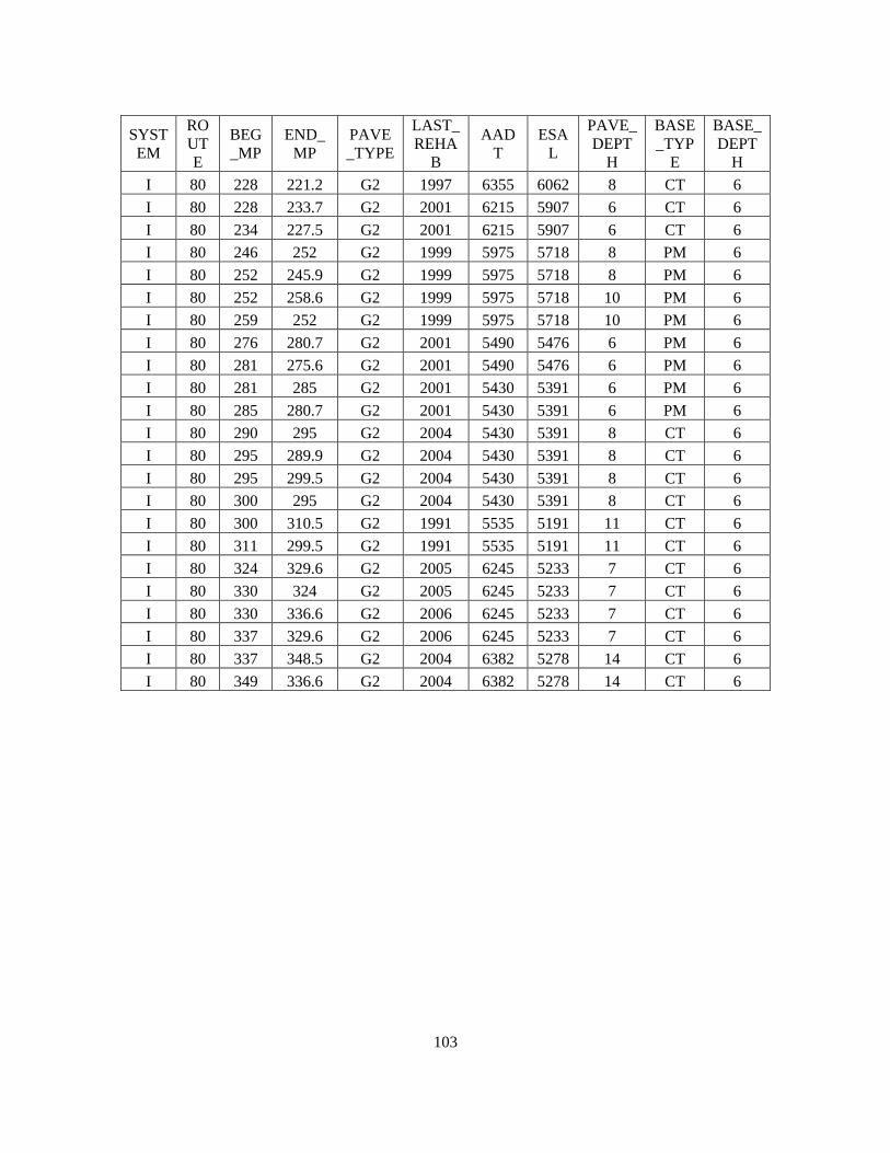
103
SYST
EM
RO
UT
E
BEG
_MP
END_
MP
PAVE
_TYPE
LAST_
REHA
B
AAD
T
ESA
L
PAVE_
DEPT
H
BASE
_TYP
E
BASE_
DEPT
H
I 80 228 221.2 G2 1997 6355 6062 8 CT 6
I 80 228 233.7 G2 2001 6215 5907 6 CT 6
I 80 234 227.5 G2 2001 6215 5907 6 CT 6
I 80 246 252 G2 1999 5975 5718 8 PM 6
I 80 252 245.9 G2 1999 5975 5718 8 PM 6
I 80 252 258.6 G2 1999 5975 5718 10 PM 6
I 80 259 252 G2 1999 5975 5718 10 PM 6
I 80 276 280.7 G2 2001 5490 5476 6 PM 6
I 80 281 275.6 G2 2001 5490 5476 6 PM 6
I 80 281 285 G2 2001 5430 5391 6 PM 6
I 80 285 280.7 G2 2001 5430 5391 6 PM 6
I 80 290 295 G2 2004 5430 5391 8 CT 6
I 80 295 289.9 G2 2004 5430 5391 8 CT 6
I 80 295 299.5 G2 2004 5430 5391 8 CT 6
I 80 300 295 G2 2004 5430 5391 8 CT 6
I 80 300 310.5 G2 1991 5535 5191 11 CT 6
I 80 311 299.5 G2 1991 5535 5191 11 CT 6
I 80 324 329.6 G2 2005 6245 5233 7 CT 6
I 80 330 324 G2 2005 6245 5233 7 CT 6
I 80 330 336.6 G2 2006 6245 5233 7 CT 6
I 80 337 329.6 G2 2006 6245 5233 7 CT 6
I 80 337 348.5 G2 2004 6382 5278 14 CT 6
I 80 349 336.6 G2 2004 6382 5278 14 CT 6

104
0
2
4
6
8
10
12
14
16
18
20
CT
PM CT
PM
PM CT
CT
PM
PM CT
CT
CT
PM CT
PM CT
CT
PM
PM CT
PM
PM CT
CT
CT
BASE TYPE
Base Depth (in)
PavementDepth (in)

105
APPENDIX B5: WYDOT BINDER GRADES

106
107
APPENDIX C1: PREDICTED DISTRESSES FOR DIFFERENT BINDER GRADES
Pavement #1 Structural Layers
Layer 1- 3in Asphalt Concrete - PG76-28
Layer 2- 3in Asphalt Concrete - PG64-28
Layer 3- 6in Asphalt Permeable Base - PG64-28
Layer 4- Subgrade (Classification A3; R-value – 42)
Table C1.1 Predicted Distresses for Pavement #1 at Big Piney
Performance Criteria Distress
Target
Reliability
Target
Distress
Predicted
Reliability
Predicted Acceptable
Terminal IRI (in/mi) 190 90 123.3 97.60 Pass
Longitudinal Cracking (ft/mi) 2000 90 0.1 99.99 Pass
Alligator Cracking (%) 25 90 0.1 99.99 Pass
Transverse Cracking (ft/mi) 1000 90 1595.1 2.34 Fail
AC Deformation (in) 0.25 90 0.1 99.99 Pass
Total Pavement Deformation (in) 0.75 90 0.24 99.99 Pass
Pavement #2 Structural Layers
Layer 1- 3in Asphalt Concrete - PG52-28
Layer 2- 3in Asphalt Concrete - PG52-28
Layer 3- 6in Asphalt Permeable Base - PG52-28
Layer 4- Subgrade (Classification A3; R-value – 42)
Table C1.2 Predicted Distresses for Pavement #2 at Big Piney
Performance Criteria Distress
Target
Reliability
Target
Distress
Predicted
Reliability
Predicted Acceptable
Terminal IRI (in/mi) 190 90 124.8 97.26 Pass
Longitudinal Cracking (ft/mi) 2000 90 4.1 99.97 Pass
Alligator Cracking (%) 25 90 0.1 99.99 Pass
Transverse Cracking (ft/mi) 1000 90 1288.4 12.83 Fail
AC Deformation (in) 0.25 90 0.19 81.56 Fail
Total Pavement Deformation (in) 0.75 90 0.34 99.99 Pass
Pavement #3 Structural Layers
Layer 1- 3in Asphalt Concrete - PG52-22
Layer 2- 3in Asphalt Concrete - PG52-22
Layer 3- 6in Asphalt Permeable Base - PG52-22
Layer 4- Subgrade (Classification A3; R-value – 42)

108
Table C1.3 Maximum values of Predicted Distresses for Pavement #3 at Big Piney
Performance Criteria Distress
Target
Reliability
Target
Distress
Predicted
Reliability
Predicted Acceptable
Terminal IRI (in/mi) 190 90 127.2 96.57 Pass
Longitudinal Cracking (ft/mi) 2000 90 2.6 99.99 Pass
Alligator Cracking (%) 25 90 0.1 99.99 Pass
Transverse Cracking (ft/mi) 1000 90 1696.9 1.33 Fail
AC Deformation (in) 0.25 90 0.17 89.58 Fail
Total Pavement Deformation (in) 0.75 90 0.32 99.99 Pass
Pavement #4 Structural Layers
Layer 1- 3in Asphalt Concrete - PG58-22
Layer 2- 3in Asphalt Concrete - PG58-22
Layer 3- 6in Asphalt Permeable Base - PG58-22
Layer 4- Subgrade (Classification A3; R-value – 42)
Table C1.4 Maximum Distresses of Predicted Distresses for Pavement #4 at Big Piney
Performance Criteria Distress
Target
Reliability
Target
Distress
Predicted
Reliability
Predicted Acceptable
Terminal IRI (in/mi) 190 90 126 96.89 Pass
Longitudinal Cracking (ft/mi) 2000 90 0.6 99.99 Pass
Alligator Cracking (%) 25 90 0.1 99.99 Pass
Transverse Cracking (ft/mi) 1000 90 1778.9 0.85 Fail
AC Deformation (in) 0.25 90 0.13 99.08 Pass
Total Pavement Deformation (in) 0.75 90 0.28 99.99 Pass
Pavement #5 Structural Layers
Layer 1- 3in Asphalt Concrete - PG64-22
Layer 2- 3in Asphalt Concrete - PG58-22
Layer 3- 6in Asphalt Permeable Base - PG58-22
Layer 4- Subgrade (Classification A3; R-value – 42)

109
Table C1.5 Maximum values of Predicted Distresses for Pavement #5 at Big Piney
Performance Criteria Distress
Target
Reliability
Target
Distress
Predicted
Reliability
Predicted Acceptable
Terminal IRI (in/mi) 190 90 125.5 97.04 Pass
Longitudinal Cracking (ft/mi) 2000 90 0.2 99.99 Pass
Alligator Cracking (%) 25 90 0.1 99.99 Pass
Transverse Cracking (ft/mi) 1000 90 1791.3 0.79 Fail
AC Deformation (in) 0.25 90 0.12 99.83 Pass
Total Pavement Deformation (in) 0.75 90 0.26 99.99 Pass
#6 Structural Layers (Big Piney Weather Station Only)
Layer 1- 3in Asphalt Concrete - PG70-22
Layer 2- 3in Asphalt Concrete - PG58-22
Layer 3- 6in Asphalt Permeable Base - PG58-22
Layer 4- Subgrade (Classification A3; R-value – 42)
Table C1.6 Maximum values of Predicted Distresses for Pavement #6 at Big Piney
Performance Criteria Distress
Target
Reliability
Target
Distress
Predicted
Reliability
Predicted Acceptable
Terminal IRI (in/mi) 190 90 125.2 97.12 Pass
Longitudinal Cracking (ft/mi) 2000 90 0.1 99.99 Pass
Alligator Cracking (%) 25 90 0.1 99.99 Pass
Transverse Cracking (ft/mi) 1000 90 1812 0.71 Fail
AC Deformation (in) 0.25 90 0.11 99.97 Pass
Total Pavement Deformation (in) 0.75 90 0.25 99.99 Pass

110

111
APPENDIX D1: PREDICTED DISTRESSES FOR INTERSTATE SYSTEM

112
TERMINAL IRI (in/mi)
Actual
Weather
Data
Virtual
Weather data
interpolated
from all
generated
stations
Diff
Actual
Weather
Data
Virtual
Weather data
interpolated
using similar
elevations
Diff
Virtual
Weather data
interpolated
from all
generated
stations
Virtual
Weather data
interpolated
using similar
elevations
Diff
IRI-1 IRI-2 IRI1-2 IRI-1 IRI-3 IRI1-3 IRI-2 IRI-3 IRI2-3
Big Piney 124.8 121.1 3.700
124.8 112 12.800
121.1 112 9.100
Buffalo 120.3 127.1 -6.800
120.3 120.6 -0.300
127.1 120.6 6.500
Casper Na 121.5 120.6 0.900
121.5 120.8 0.700
120.6 120.8 -0.200
Cheyenne 114.3 122.1 -7.800
114.3 115.5 -1.200
122.1 115.5 6.600
Doug. Avn 121.8 119.4 2.400
121.8 120.3 1.500
119.4 120.3 -0.900
Evanston 112.5 117.2 -4.700
112.5 122.2 -9.700
117.2 122.2 -5.000
Gillette 122.0 119.1 2.900
122.0 119.4 2.600
119.1 119.4 -0.300
Greybull 126.0 124.3 1.700
126.0 125.8 0.200
124.3 125.8 -1.500
Lander 121.3 120.6 0.700
121.3 121.2 0.100
120.6 121.2 -0.600
Laramie 117.7 119.3 -1.600
117.7 118.3 -0.600
119.3 118.3 1.000
Rawlins 117.5 120.2 -2.700
117.5 112.5 5.000
120.2 112.5 7.700
Riverton 121.2 121.2 0.000
121.2 121.3 -0.100
121.2 121.3 -0.100
Rock
Springs 113.6 119.5 -5.900
113.6 120.1 -6.500
119.5 120.1 -0.600
Sheridan 123.4 126.2 -2.800
123.4 126.4 -3.000
126.2 126.4 -0.200
Worland 129.9 119.6 10.300
129.9 125.2 4.700
119.6 125.2 -5.600
IRI-1 International Roughness Index from Actual Weather Data.
IRI-2 International Roughness Index from Virtual Weather Data generated by interpolation using all neighboring stations.
IRI-3 International Roughness Index from Virtual Weather Data generated by interpolation using stations with similar elevation.

113
AC SURFACE DOWN CRACKING (LONGITUDINAL CRACKING) (ft/mile)
Actual
Weather
Data
Virtual
Weather data
interpolated
from all
generated
stations
Diff
Actual
Weather
Data
Virtual
Weather data
interpolated
using similar
elevations
Diff
Virtual
Weather data
interpolated
from all
generated
stations
Virtual
Weather data
interpolated
using similar
elevations
Diff
LC-1 LC-2 LC1-2 LC-1 LC-3 LC1-3
LC-2 LC-3 LC2-3
Big Piney 4.1 4.6 -0.500
4.1 5.5 -1.400
4.6 5.5 -0.900
Buffalo 10.3 5.7 4.600
10.3 7.3 3.000
5.7 7.3 -1.600
Casper Na 10.0 9.8 0.200
10.0 9.4 0.600
9.8 9.4 0.400
Cheyenne 2.3 1.8 0.500
2.3 1.9 0.400
1.8 1.9 -0.100
Doug. Avn 14.3 7.0 7.300
14.3 10.3 4.000
7.0 10.3 -3.300
Evanston 3.5 2.5 1.000
3.5 9 -5.500
2.5 9 -6.500
Gillette 12.0 7.6 4.400
12.0 9.6 2.400
7.6 9.6 -2.000
Greybull 81.5 10.8 70.700
81.5 24.3 57.200
10.8 24.3 -13.500
Lander 19.5 15.6 3.900
19.5 18.2 1.300
15.6 18.2 -2.600
Laramie 3.1 1.0 2.100
3.1 5.8 -2.700
1.0 5.8 -4.800
Rawlins 7.3 3.5 3.800
7.3 5.3 2.000
3.5 5.3 -1.800
Riverton 17.9 16.3 1.600
17.9 19.3 -1.400
16.3 19.3 -3.000
Rock
Springs 11.1 6.3 4.800
11.1 4.9 6.200
6.3 4.9 1.400
Sheridan 15.4 12.3 3.100
15.4 15.6 -0.200
12.3 15.6 -3.300
Worland 72.2 20.5 51.700
72.2 32.5 39.700
20.5 32.5 -12.000
LC-1 Longitudinal Cracking from Actual Weather Data.
LC-2 Longitudinal Cracking from Virtual Weather Data generated by interpolation using all neighboring stations.
LC-3 Longitudinal Cracking from Virtual Weather Data generated by interpolation using stations with similar elevation.

114
AC BOTTOM UP CRACKING (ALLIGATOR CRACKING) (%)
Actual
Weather
Data
Virtual
Weather data
interpolated
from all
generated
stations
Diff
Actual
Weather
Data
Virtual
Weather data
interpolated
using similar
elevations
Diff
Virtual
Weather data
interpolated
from all
generated
stations
Virtual
Weather data
interpolated
using similar
elevations
Diff
AC-1 AC-2 AC1-2 AC-1 AC-3 AC1-3
AC-2 AC-3 AC2-3
Big Piney 0.1 0.1 0.000
0.1 0.1 0.000
0.1 0.1 0.000
Buffalo 0.2 0.1 0.100
0.2 0.2 0.000
0.1 0.2 -0.100
Casper Na 0.2 0.2 0.000
0.2 0.2 0.000
0.2 0.2 0.000
Cheyenne 0.1 0.1 0.000
0.1 0.1 0.000
0.1 0.1 0.000
Doug. Avn 0.2 0.2 0.000
0.2 0.2 0.000
0.2 0.2 0.000
Evanston 0.1 0.1 0.000
0.1 0.1 0.000
0.1 0.1 0.000
Gillette 0.2 0.2 0.000
0.2 0.2 0.000
0.2 0.2 0.000
Greybull 0.2 0.2 0.000
0.2 0.2 0.000
0.2 0.2 0.000
Lander 0.2 0.2 0.000
0.2 0.2 0.000
0.2 0.2 0.000
Laramie 0.1 0.1 0.000
0.1 0.1 0.000
0.1 0.1 0.000
Rawlins 0.1 0.1 0.000
0.1 0.1 0.000
0.1 0.1 0.000
Riverton 0.2 0.2 0.000
0.2 0.2 0.000
0.2 0.2 0.000
Rock
Springs 0.1 0.1 0.000
0.1 0.1 0.000
0.1 0.1 0.000
Sheridan 0.2 0.2 0.000
0.2 0.2 0.000
0.2 0.2 0.000
Worland 0.2 0.2 0.000
0.2 0.2 0.000
0.2 0.2 0.000
AC-1 Alligator Cracking from Actual Weather Data.
AC-2 Alligator Cracking from Virtual Weather Data generated by interpolation using all neighboring stations.
AC-3 Alligator Cracking from Virtual Weather Data generated by interpolation using stations with similar elevation.

115
THERMAL FRACTURE (TRANSVERSE CRACKING) (ft/mi)
Actual
Weather
Data
Virtual
Weather data
interpolated
from all
generated
stations
Diff
Actual
Weather
Data
Virtual
Weather
data
interpolated
using
similar
elevations
Diff
Virtual
Weather data
interpolated
from all
generated
stations
Virtual
Weather data
interpolated
using similar
elevations
Diff
TC-1 TC-2 TC1-2 TC-1 TC-3 TC1-3
TC-2 TC-3 TC2-3
Big Piney 1289.2 826.7 462.500
1288.4 4.6 1283.800
826.7 4.6 822.100
Buffalo 697.2 1496.6 -799.400
697.2 809.5 -112.300
1496.6 809.5 687.100
Casper Na 861.0 711.3 149.700
861.0 735.6 125.400
711.3 735.6 -24.300
Cheyenne 154.8 1117.7 -962.900
154.8 382.1 -227.300
1117.7 382.1 735.600
Doug. Avn 747.5 649.9 97.600
747.5 724.1 23.400
649.9 724.1 -74.200
Evanston 3.1 339.8 -336.700
3.1 1072.4 -1069.300
339.8 1072.4 -732.600
Gillette 776.9 516.8 260.100
776.9 530.2 246.700
516.8 530.2 -13.400
Greybull 1051.0 1032.1 18.900
1051.0 1024.3 26.700
1032.1 1024.3 7.800
Lander 530.5 672.4 -141.900
530.5 702.7 -172.200
672.4 702.7 -30.300
Laramie 780.5 864 -83.500
780.5 775.7 4.800
864 775.7 88.300
Rawlins 588.1 826 -237.900
588.1 99.4 488.700
826 99.4 726.600
Riverton 716.9 584.8 132.100
716.9 537.5 179.400
584.8 537.5 47.300
Rock
Springs 57.7 751.6 -693.900
57.7 986.4 -928.700
751.6 986.4 -234.800
Sheridan 740.1 1405.7 -665.600
740.1 1411.4 -671.300
1405.7 1411.4 -5.700
Worland 1294.8 401.6 893.200
1294.8 1059.7 235.100
401.6 1059.7 -658.100
TC-1 Transverse Cracking from Actual Weather Data.
TC-2 Transverse Cracking from Virtual Weather Data generated by interpolation using all neighboring stations.
TC-3 Transverse Cracking from Virtual Weather Data generated by interpolation using stations with similar elevation.

116
PERMANENT DEFORMATION (HMA LAYER) (in)
Actual
Weather
Data
Virtual
Weather data
interpolated
from all
generated
stations
Diff
Actual
Weather
Data
Virtual
Weather data
interpolated
using similar
elevations
Diff
Virtual
Weather data
interpolated
from all
generated
stations
Virtual
Weather data
interpolated
using similar
elevations
Diff
ACR-1 ACR-2 ACR1-2 ACR-1 ACR-3 ACR1-3
ACR-2 ACR-3 ACR2-3
Big Piney 0.19 0.21 -0.020
0.19 0.19 0.000
0.21 0.19 0.020
Buffalo 0.24 0.22 0.020
0.24 0.22 0.020
0.22 0.22 0.000
Casper Na 0.24 0.24 0.000
0.24 0.24 0.000
0.24 0.24 0.000
Cheyenne 0.19 0.18 0.010
0.19 0.18 0.010
0.18 0.18 0.000
Doug. Avn 0.26 0.23 0.030
0.26 0.24 0.020
0.23 0.24 -0.010
Evanston 0.18 0.19 -0.010
0.18 0.21 -0.030
0.19 0.21 -0.020
Gillette 0.25 0.24 0.010
0.25 0.24 0.010
0.24 0.24 0.000
Greybull 0.34 0.26 0.080
0.34 0.29 0.050
0.26 0.29 -0.030
Lander 0.28 0.25 0.030
0.28 0.26 0.020
0.25 0.26 -0.010
Laramie 0.17 0.16 0.010
0.17 0.19 -0.020
0.16 0.19 -0.030
Rawlins 0.20 0.20 0.000
0.20 0.19 0.010
0.20 0.19 0.010
Riverton 0.26 0.27 -0.010
0.26 0.28 -0.020
0.27 0.28 -0.010
Rock
Springs 0.22 0.21 0.010
0.22 0.18 0.040
0.21 0.18 0.030
Sheridan 0.28 0.25 0.030
0.28 0.25 0.030
0.25 0.25 0.000
Worland 0.35 0.28 0.070
0.35 0.29 0.060
0.28 0.29 -0.010
ACR-1 AC Rutting from Actual Weather Data.
ACR-2 AC Rutting from Virtual Weather Data generated by interpolation using all neighboring stations.
ACR-3 AC Rutting from Virtual Weather Data generated by interpolation using stations with similar elevation.

117
TOTAL PAVEMENT DEFORMATION (in)
Actual
Weather
Data
Virtual
Weather data
interpolated
from all
generated
stations
Diff
Actual
Weather
Data
Virtual
Weather data
interpolated
using similar
elevations
Diff
Virtual
Weather data
interpolated
from all
generated
stations
Virtual
Weather data
interpolated
using similar
elevations
Diff
TR-1 TR-2 TR1-2 TR-1 TR-3 TR1-3
TR-2 TR-3 TR2-3
Big Piney 0.34 0.36 -0.020
0.34 0.33 0.010
0.36 0.33 0.030
Buffalo 0.38 0.37 0.010
0.38 0.37 0.010
0.37 0.37 0.000
Casper Na 0.39 0.39 0.000
0.39 0.39 0.000
0.39 0.39 0.000
Cheyenne 0.34 0.33 0.010
0.34 0.32 0.020
0.33 0.32 0.010
Doug. Avn 0.41 0.37 0.040
0.41 0.39 0.020
0.37 0.39 -0.020
Evanston 0.32 0.34 -0.020
0.32 0.35 -0.030
0.34 0.35 -0.010
Gillette 0.40 0.39 0.010
0.40 0.39 0.010
0.39 0.39 0.000
Greybull 0.48 0.41 0.070
0.48 0.45 0.030
0.41 0.45 -0.040
Lander 0.43 0.40 0.030
0.43 0.41 0.020
0.40 0.41 -0.010
Laramie 0.31 0.31 0.000
0.31 0.33 -0.020
0.31 0.33 -0.020
Rawlins 0.34 0.34 0.000
0.34 0.32 0.020
0.34 0.32 0.020
Riverton 0.41 0.42 -0.010
0.41 0.43 -0.020
0.42 0.43 -0.010
Rock
Springs 0.36 0.35 0.010
0.36 0.32 0.040
0.35 0.32 0.030
Sheridan 0.43 0.40 0.030
0.43 0.4 0.030
0.40 0.4 0.000
Worland 0.50 0.43 0.070
0.50 0.44 0.060
0.43 0.44 -0.010
TR-1 Total Rutting from Actual Weather Data.
TR-2 Total Rutting from Virtual Weather Data generated by interpolation using all neighboring stations.
TR-3 Total Rutting from Virtual Weather Data generated by interpolation using stations with similar elevation.

118
Actual
Weather
Data
Virtual
Weather
data
interpolated
from all
generated
stations
Change
Actual
Weather
Data
Virtual
Weather
data
interpolated
using
similar
elevations
Change
Virtual
Weather
data
interpolated
from all
generated
stations
Virtual
Weather
data
interpolated
using
similar
elevations
Change
IRI-1 IRI-2 IRI1-2 IRI-1 IRI-3 IRI1-3 IRI-2 IRI-3 IRI2-3
Big Piney 124.8 121.1 -0.030
124.8 112 -0.103
121.1 112 -0.075
Buffalo 120.3 127.1 0.057
120.3 120.6 0.002
127.1 120.6 -0.051
Casper Na 121.5 120.6 -0.007
121.5 120.8 -0.006
120.6 120.8 0.002
Cheyenne 114.3 122.1 0.068
114.3 115.5 0.010
122.1 115.5 -0.054
Doug. Avn 121.8 119.4 -0.020
121.8 120.3 -0.012
119.4 120.3 0.008
Evanston 112.5 117.2 0.042
112.5 122.2 0.086
117.2 122.2 0.043
Gillette 122.0 119.1 -0.024
122.0 119.4 -0.021
119.1 119.4 0.003
Greybull 126.0 124.3 -0.013
126.0 125.8 -0.002
124.3 125.8 0.012
Lander 121.3 120.6 -0.006
121.3 121.2 -0.001
120.6 121.2 0.005
Laramie 117.7 119.3 0.014
117.7 118.3 0.005
119.3 118.3 -0.008
Rawlins 117.5 120.2 0.023
117.5 112.5 -0.043
120.2 112.5 -0.064
Riverton 121.2 121.2 0.000
121.2 121.3 0.001
121.2 121.3 0.001
Rock
Springs 113.6 119.5 0.052
113.6 120.1 0.057
119.5 120.1 0.005
Sheridan 123.4 126.2 0.023
123.4 126.4 0.024
126.2 126.4 0.002
Worland 129.9 119.6 -0.079
129.9 125.2 -0.036
119.6 125.2 0.047

119
Actual
Weather
Data
Virtual
Weather data
interpolated
from all
generated
stations
Change
Actual
Weather
Data
Virtual
Weather
data
interpolated
using
similar
elevations
Change
Virtual
Weather data
interpolated
from all
generated
stations
Virtual
Weather
data
interpolated
using
similar
elevations
Change
LC-1 LC-2 LC1-2 LC-1 LC-3 LC1-3 LC-2 LC-3 LC2-3
Big Piney 4.1 4.6 0.122 4.1 5.5 0.341 4.6 5.5 0.196
Buffalo 10.3 5.7 -0.447 10.3 7.3 -0.291 5.7 7.3 0.281
Casper Na 10.0 9.8 -0.020 10.0 9.4 -0.060 9.8 9.4 -0.041
Cheyenne 2.3 1.8 -0.217 2.3 1.9 -0.174 1.8 1.9 0.056
Doug. Avn 14.3 7.0 -0.510 14.3 10.3 -0.280 7.0 10.3 0.471
Evanston 3.5 2.5 -0.286 3.5 9 1.571 2.5 9 2.600
Gillette 12.0 7.6 -0.367 12.0 9.6 -0.200 7.6 9.6 0.263
Greybull 81.5 10.8 -0.867 81.5 24.3 -0.702 10.8 24.3 1.250
Lander 19.5 15.6 -0.200 19.5 18.2 -0.067 15.6 18.2 0.167
Laramie 3.1 1.0 -0.677 3.1 5.8 0.871 1.0 5.8 4.800
Rawlins 7.3 3.5 -0.521 7.3 5.3 -0.274 3.5 5.3 0.514
Riverton 17.9 16.3 -0.089 17.9 19.3 0.078 16.3 19.3 0.184
Rock
Springs 11.1 6.3 -0.432
11.1 4.9 -0.559
6.3 4.9 -0.222
Sheridan 15.4 12.3 -0.201 15.4 15.6 0.013 12.3 15.6 0.268
Worland 72.2 20.5 -0.716 72.2 32.5 -0.550 20.5 32.5 0.585

120
Actual
Weather
Data
Virtual
Weather data
interpolated
from all
generated
stations
Change
Actual
Weather
Data
Virtual
Weather
data
interpolated
using similar
elevations
Change
Virtual
Weather data
interpolated
from all
generated
stations
Virtual
Weather
data
interpolated
using similar
elevations
Change
AC-1 AC-2 AC1-2 AC-1 AC-3 AC1-3 AC-2 AC-3 AC2-3
Big Piney 0.1 0.1 0.000 0.1 0.1 0.000 0.1 0.1 0.000
Buffalo 0.2 0.1 -0.500 0.2 0.2 0.000 0.1 0.2 1.000
Casper Na 0.2 0.2 0.000 0.2 0.2 0.000 0.2 0.2 0.000
Cheyenne 0.1 0.1 0.000 0.1 0.1 0.000 0.1 0.1 0.000
Doug. Avn 0.2 0.2 0.000 0.2 0.2 0.000 0.2 0.2 0.000
Evanston 0.1 0.1 0.000 0.1 0.1 0.000 0.1 0.1 0.000
Gillette 0.2 0.2 0.000 0.2 0.2 0.000 0.2 0.2 0.000
Greybull 0.2 0.2 0.000 0.2 0.2 0.000 0.2 0.2 0.000
Lander 0.2 0.2 0.000 0.2 0.2 0.000 0.2 0.2 0.000
Laramie 0.1 0.1 0.000 0.1 0.1 0.000 0.1 0.1 0.000
Rawlins 0.1 0.1 0.000 0.1 0.1 0.000 0.1 0.1 0.000
Riverton 0.2 0.2 0.000 0.2 0.2 0.000 0.2 0.2 0.000
Rock
Springs 0.1 0.1 0.000
0.1 0.1 0.000
0.1 0.1 0.000
Sheridan 0.2 0.2 0.000 0.2 0.2 0.000 0.2 0.2 0.000
Worland 0.2 0.2 0.000 0.2 0.2 0.000 0.2 0.2 0.000

121
Actual
Weather
Data
Virtual
Weather
data
interpolated
from all
generated
stations
Change
Actual
Weather
Data
Virtual
Weather
data
interpolated
using
similar
elevations
Change
Virtual
Weather data
interpolated
from all
generated
stations
Virtual
Weather
data
interpolated
using
similar
elevations
Change
TC-1 TC-2 TC1-2 TC-1 TC-3 TC1-3 TC-2 TC-3 TC2-3
Big Piney 1289.2 826.7 -0.359 1288.4 4.6 -0.996 826.7 4.6 -0.994
Buffalo 697.2 1496.6 1.147 697.2 809.5 0.161 1496.6 809.5 -0.459
Casper Na 861.0 711.3 -0.174 861.0 735.6 -0.146 711.3 735.6 0.034
Cheyenne 154.8 1117.7 6.220 154.8 382.1 1.468 1117.7 382.1 -0.658
Doug. Avn 747.5 649.9 -0.131 747.5 724.1 -0.031 649.9 724.1 0.114
Evanston 3.1 339.8 108.613 3.1 1072.4 344.935 339.8 1072.4 2.156
Gillette 776.9 516.8 -0.335 776.9 530.2 -0.318 516.8 530.2 0.026
Greybull 1051.0 1032.1 -0.018 1051.0 1024.3 -0.025 1032.1 1024.3 -0.008
Lander 530.5 672.4 0.267 530.5 702.7 0.325 672.4 702.7 0.045
Laramie 780.5 864 0.107 780.5 775.7 -0.006 864 775.7 -0.102
Rawlins 588.1 826 0.405 588.1 99.4 -0.831 826 99.4 -0.880
Riverton 716.9 584.8 -0.184 716.9 537.5 -0.250 584.8 537.5 -0.081
Rock
Springs 57.7 751.6 12.026
57.7 986.4 16.095
751.6 986.4 0.312
Sheridan 740.1 1405.7 0.899 740.1 1411.4 0.907 1405.7 1411.4 0.004
Worland 1294.8 401.6 -0.690 1294.8 1059.7 -0.182 401.6 1059.7 1.639

122
Actual
Weather
Data
Virtual
Weather data
interpolated
from all
generated
stations
Change
Actual
Weather
Data
Virtual
Weather
data
interpolated
using
similar
elevations
Change
Virtual
Weather data
interpolated
from all
generated
stations
Virtual
Weather
data
interpolated
using
similar
elevations
Change
ACR-1 ACR-2 ACR1-2 ACR-1 ACR-3 ACR1-3 ACR-2 ACR-3 ACR2-3
Big Piney 0.19 0.21 0.105 0.19 0.19 0.000 0.21 0.19 -0.095
Buffalo 0.24 0.22 -0.083 0.24 0.22 -0.083 0.22 0.22 0.000
Casper Na 0.24 0.24 0.000 0.24 0.24 0.000 0.24 0.24 0.000
Cheyenne 0.19 0.18 -0.053 0.19 0.18 -0.053 0.18 0.18 0.000
Doug. Avn 0.26 0.23 -0.115 0.26 0.24 -0.077 0.23 0.24 0.043
Evanston 0.18 0.19 0.056 0.18 0.21 0.167 0.19 0.21 0.105
Gillette 0.25 0.24 -0.040 0.25 0.24 -0.040 0.24 0.24 0.000
Greybull 0.34 0.26 -0.235 0.34 0.29 -0.147 0.26 0.29 0.115
Lander 0.28 0.25 -0.107 0.28 0.26 -0.071 0.25 0.26 0.040
Laramie 0.17 0.16 -0.059 0.17 0.19 0.118 0.16 0.19 0.188
Rawlins 0.20 0.20 0.000 0.20 0.19 -0.050 0.20 0.19 -0.050
Riverton 0.26 0.27 0.038 0.26 0.28 0.077 0.27 0.28 0.037
Rock
Springs 0.22 0.21 -0.045
0.22 0.18 -0.182
0.21 0.18 -0.143
Sheridan 0.28 0.25 -0.107 0.28 0.25 -0.107 0.25 0.25 0.000
Worland 0.35 0.28 -0.200 0.35 0.29 -0.171 0.28 0.29 0.036

123
Actual
Weather
Data
Virtual
Weather data
interpolated
from all
generated
stations
Change
Actual
Weather
Data
Virtual
Weather
data
interpolated
using
similar
elevations
Change
Virtual
Weather data
interpolated
from all
generated
stations
Virtual
Weather
data
interpolated
using
similar
elevations
Change
TR-1 TR-2 TR1-2 TR-1 TR-3 TR1-3 TR-2 TR-3 TR2-3
Big Piney 0.34 0.36 0.059 0.34 0.33 -0.029 0.36 0.33 -0.083
Buffalo 0.38 0.37 -0.026 0.38 0.37 -0.026 0.37 0.37 0.000
Casper Na 0.39 0.39 0.000 0.39 0.39 0.000 0.39 0.39 0.000
Cheyenne 0.34 0.33 -0.029 0.34 0.32 -0.059 0.33 0.32 -0.030
Doug. Avn 0.41 0.37 -0.098 0.41 0.39 -0.049 0.37 0.39 0.054
Evanston 0.32 0.34 0.063 0.32 0.35 0.094 0.34 0.35 0.029
Gillette 0.40 0.39 -0.025 0.40 0.39 -0.025 0.39 0.39 0.000
Greybull 0.48 0.41 -0.146 0.48 0.45 -0.062 0.41 0.45 0.098
Lander 0.43 0.40 -0.070 0.43 0.41 -0.047 0.40 0.41 0.025
Laramie 0.31 0.31 0.000 0.31 0.33 0.065 0.31 0.33 0.065
Rawlins 0.34 0.34 0.000 0.34 0.32 -0.059 0.34 0.32 -0.059
Riverton 0.41 0.42 0.024 0.41 0.43 0.049 0.42 0.43 0.024
Rock
Springs 0.36 0.35 -0.028
0.36 0.32 -0.111
0.35 0.32 -0.086
Sheridan 0.43 0.40 -0.070 0.43 0.4 -0.070 0.40 0.4 0.000
Worland 0.50 0.43 -0.140 0.50 0.44 -0.120 0.43 0.44 0.023

124

125
APPENDIX D2: ANNUAL CLIMATE STATISTICS

126
MEAN ANNUAL AIR TEMPERATURE (F)
Actual
Weather
Data
Virtual
Weather data
interpolated
from all
generated
stations
Diff
Actual
Weather
Data
Virtual
Weather data
interpolated
using similar
elevations
Diff
Virtual
Weather data
interpolated
from all
generated
stations
Virtual
Weather data
interpolated
using similar
elevations
Diff
AT-1 AT-2 AT1-2 AT-1 AT-3 AT1-3
AT-2 AT-3 AT2-3
Big Piney 37.19 40.90 -3.710
37.19 43.29 -6.100
40.90 43.29 -2.390
Buffalo 46.79 43.06 3.730
46.79 45.98 0.810
43.06 45.98 -2.920
Casper Na 46.26 45.47 0.790
46.26 45.36 0.900
45.47 45.36 0.110
Cheyenne 46.86 43.70 3.160
46.86 46.81 0.050
43.70 46.81 -3.110
Doug. Avn 46.61 47.04 -0.430
46.61 47.26 -0.650
47.04 47.26 -0.220
Evanston 42.29 40.54 1.750
42.29 38.84 3.450
40.54 38.84 1.700
Gillette 47.11 47.05 0.060
47.11 47.01 0.100
47.05 47.01 0.040
Greybull 46.20 47.26 -1.060
46.20 46.13 0.070
47.26 46.13 1.130
Lander 45.80 45.02 0.780
45.80 45.2 0.600
45.02 45.2 -0.180
Laramie 41.96 41.44 0.520
41.96 42.2 -0.240
41.44 42.2 -0.760
Rawlins 43.95 41.73 2.220
43.95 43.92 0.030
41.73 43.92 -2.190
Riverton 45.20 45.13 0.070
45.20 45.8 -0.600
45.13 45.8 -0.670
Rock
Springs 43.95 41.31 2.640
43.95 40.77 3.180
41.31 40.77 0.540
Sheridan 45.92 48.15 -2.230
45.92 46.61 -0.690
48.15 46.61 1.540
Worland 45.54 47.39 -1.850
45.54 45.27 0.270
47.39 45.27 2.120

127
MEAN ANNUAL RAINFALL (in)
Actual
Weather
Data
Virtual
Weather data
interpolated
from all
generated
stations
Diff
Actual
Weather
Data
Virtual
Weather data
interpolated
using similar
elevations
Diff
Virtual
Weather data
interpolated
from all
generated
stations
Virtual
Weather data
interpolated
using similar
elevations
Diff
AR-1 AR-2 AR1-2 AR-1 AR-3 AR1-3
AR-2 AR-3 AR2-3
Big Piney 12.15 11.68 0.470
12.15 8.03 4.120
11.68 8.03 3.650
Buffalo 11.90 12.80 -0.900
11.90 10.98 0.920
12.80 10.98 1.820
Casper Na 10.40 10.70 -0.300
10.40 10.73 -0.330
10.70 10.73 -0.030
Cheyenne 13.26 13.32 -0.060
13.26 12.74 0.520
13.32 12.74 0.580
Doug. Avn 11.86 11.33 0.530
11.86 10.56 1.300
11.33 10.56 0.770
Evanston 10.49 14.13 -3.640
10.49 7.84 2.650
14.13 7.84 6.290
Gillette 12.85 12.75 0.100
12.85 12.2 0.650
12.75 12.2 0.550
Greybull 5.27 12.46 -7.190
5.27 11.78 -6.510
12.46 11.78 0.680
Lander 11.42 8.82 2.600
11.42 8.4 3.020
8.82 8.4 0.420
Laramie 8.82 12.94 -4.120
8.82 7.98 0.840
12.94 7.98 4.960
Rawlins 9.07 10.94 -1.870
9.07 7.91 1.160
10.94 7.91 3.030
Riverton 8.46 11.28 -2.820
8.46 11.36 -2.900
11.28 11.36 -0.080
Rock
Springs 7.94 9.25 -1.310
7.94 8.04 -0.100
9.25 8.04 1.210
Sheridan 13.85 10.90 2.950
13.85 9.43 4.420
10.90 9.43 1.470
Worland 9.69 9.87 -0.180
9.69 8.15 1.540
9.87 8.15 1.720

128
FREEZING INDEX (F-days)
Actual
Weather
Data
Virtual
Weather data
interpolated
from all
generated
stations
Diff
Actual
Weather
Data
Virtual
Weather data
interpolated
using similar
elevations
Diff
Virtual
Weather data
interpolated
from all
generated
stations
Virtual
Weather data
interpolated
using similar
elevations
Diff
FI-1 FI-2 FI1-2 FI-1 FI-3 FI1-3
FI-2 FI-3 FI2-3
Big Piney 2439.19 1655.95 783.240
2439.19 1238.36 1200.830
1655.95 1238.36 417.590
Buffalo 874.26 1459.03 -584.770
874.26 1028.5 -154.240
1459.03 1028.5 430.530
Casper Na 986.09 1124.28 -138.190
986.09 1146.45 -160.360
1124.28 1146.45 -22.170
Cheyenne 793.33 1233.91 -440.580
793.33 877.67 -84.340
1233.91 877.67 356.240
Doug. Avn 1068.48 887.24 181.240
1068.48 885.43 183.050
887.24 885.43 1.810
Evanston 1325.58 1676.79 -351.210
1325.58 2098.26 -772.680
1676.79 2098.26 -421.470
Gillette 949.71 875.94 73.770
949.71 897.47 52.240
875.94 897.47 -21.530
Greybull 1569.36 1006.47 562.890
1569.36 1175.34 394.020
1006.47 1175.34 -168.870
Lander 1187.27 1312.40 -125.130
1187.27 1315.33 -128.060
1312.40 1315.33 -2.930
Laramie 1314.61 1398.28 -83.670
1314.61 1390.44 -75.830
1398.28 1390.44 7.840
Rawlins 1162.02 1486.62 -324.600
1162.02 1128.66 33.360
1486.62 1128.66 357.960
Riverton 1315.53 1268.94 46.590
1315.53 1187.27 128.260
1268.94 1187.27 81.670
Rock
Springs 1253.80 1609.43 -355.630
1253.80 1660.99 -407.190
1609.43 1660.99 -51.560
Sheridan 1110.34 872.54 237.800
1110.34 1180.55 -70.210
872.54 1180.55 -308.010
Worland 1452.64 1080.04 372.600
1452.64 1432.15 20.490
1080.04 1432.15 -352.110

129
AVERAGE NUMBER OF FREEZE/THAW CYCLES
Actual
Weather
Data
Virtual
Weather data
interpolated
from all
generated
stations
Diff
Actual
Weather
Data
Virtual
Weather data
interpolated
using similar
elevations
Diff
Virtual
Weather data
interpolated
from all
generated
stations
Virtual
Weather
data
interpolated
using
similar
elevations
Diff
FT-1 FT-2 FT1-2 FT-1 FT-3 FT1-3
FT-2 FT-3 FT2-3
Big Piney 149 134 15.000
149 117 32.000
134 117 17.000
Buffalo 123 154 -31.000
123 138 -15.000
154 138 16.000
Casper Na 118 131 -13.000
118 138 -20.000
131 138 -7.000
Cheyenne 117 144 -27.000
117 157 -40.000
144 157 -13.000
Doug. Avn 135 121 14.000
135 128 7.000
121 128 -7.000
Evanston 98 116 -18.000
98 144 -46.000
116 144 -28.000
Gillette 124 119 5.000
124 123 1.000
119 123 -4.000
Greybull 118 116 2.000
118 150 -32.000
116 150 -34.000
Lander 124 131 -7.000
124 121 3.000
131 121 10.000
Laramie 146 146 0.000
146 152 -6.000
146 152 -6.000
Rawlins 120 136 -16.000
120 138 -18.000
136 138 -2.000
Riverton 121 138 -17.000
121 124 -3.000
138 124 14.000
Rock
Springs 111 130 -19.000
111 137 -26.000
130 137 -7.000
Sheridan 140 111 29.000
140 116 24.000
111 116 -5.000
Worland 127 114 13.000
127 133 -6.000
114 133 -19.000

130
Actual
Weather
Data
Virtual
Weather
data
interpolated
from all
generated
stations
Change
Actual
Weather
Data
Virtual
Weather
data
interpolated
using
similar
elevations
Change
Virtual
Weather
data
interpolated
from all
generated
stations
Virtual
Weather
data
interpolated
using
similar
elevations
Change
AT-1 AT-2 AT1-2 AT-1 AT-3 AT1-3 AT-2 AT-3 AT2-3
Big Piney 37.19 40.90 0.100 37.19 43.29 0.164 40.90 43.29 0.058
Buffalo 46.79 43.06 -0.080 46.79 45.98 -0.017 43.06 45.98 0.068
Casper Na 46.26 45.47 -0.017 46.26 45.36 -0.019 45.47 45.36 -0.002
Cheyenne 46.86 43.70 -0.067 46.86 46.81 -0.001 43.70 46.81 0.071
Doug. Avn 46.61 47.04 0.009 46.61 47.26 0.014 47.04 47.26 0.005
Evanston 42.29 40.54 -0.041 42.29 38.84 -0.082 40.54 38.84 -0.042
Gillette 47.11 47.05 -0.001 47.11 47.01 -0.002 47.05 47.01 -0.001
Greybull 46.20 47.26 0.023 46.20 46.13 -0.002 47.26 46.13 -0.024
Lander 45.80 45.02 -0.017 45.80 45.2 -0.013 45.02 45.2 0.004
Laramie 41.96 41.44 -0.012 41.96 42.2 0.006 41.44 42.2 0.018
Rawlins 43.95 41.73 -0.051 43.95 43.92 -0.001 41.73 43.92 0.052
Riverton 45.20 45.13 -0.002 45.20 45.8 0.013 45.13 45.8 0.015
Rock
Springs 43.95 41.31 -0.060
43.95 40.77 -0.072
41.31 40.77 -0.013
Sheridan 45.92 48.15 0.049 45.92 46.61 0.015 48.15 46.61 -0.032
Worland 45.54 47.39 0.041 45.54 45.27 -0.006 47.39 45.27 -0.045

131
Actual
Weather
Data
Virtual
Weather data
interpolated
from all
generated
stations
Change
Actual
Weather
Data
Virtual
Weather
data
interpolated
using
similar
elevations
Change
Virtual
Weather data
interpolated
from all
generated
stations
Virtual
Weather
data
interpolated
using
similar
elevations
Change
AR-1 AR-2 AR1-2 AR-1 AR-3 AR1-3 AR-2 AR-3 AR2-3
Big Piney 12.15 11.68 -0.039 12.15 8.03 -0.339 11.68 8.03 -0.313
Buffalo 11.90 12.80 0.076 11.90 10.98 -0.077 12.80 10.98 -0.142
Casper Na 10.40 10.70 0.029 10.40 10.73 0.032 10.70 10.73 0.003
Cheyenne 13.26 13.32 0.005 13.26 12.74 -0.039 13.32 12.74 -0.044
Doug. Avn 11.86 11.33 -0.045 11.86 10.56 -0.110 11.33 10.56 -0.068
Evanston 10.49 14.13 0.347 10.49 7.84 -0.253 14.13 7.84 -0.445
Gillette 12.85 12.75 -0.008 12.85 12.2 -0.051 12.75 12.2 -0.043
Greybull 5.27 12.46 1.364 5.27 11.78 1.235 12.46 11.78 -0.055
Lander 11.42 8.82 -0.228 11.42 8.4 -0.264 8.82 8.4 -0.048
Laramie 8.82 12.94 0.467 8.82 7.98 -0.095 12.94 7.98 -0.383
Rawlins 9.07 10.94 0.206 9.07 7.91 -0.128 10.94 7.91 -0.277
Riverton 8.46 11.28 0.333 8.46 11.36 0.343 11.28 11.36 0.007
Rock
Springs 7.94 9.25 0.165
7.94 8.04 0.013
9.25 8.04 -0.131
Sheridan 13.85 10.90 -0.213 13.85 9.43 -0.319 10.90 9.43 -0.135
Worland 9.69 9.87 0.019 9.69 8.15 -0.159 9.87 8.15 -0.174
132
Actual
Weather
Data
Virtual
Weather data
interpolated
from all
generated
stations
Change
Actual
Weather
Data
Virtual
Weather
data
interpolated
using
similar
elevations
Change
Virtual
Weather data
interpolated
from all
generated
stations
Virtual
Weather
data
interpolated
using
similar
elevations
Change
FI-1 FI-2 FI1-2 FI-1 FI-3 FI1-3
FI-2 FI-3 FI2-3
Big Piney 2439.19 1655.95 -0.321
2439.19 1238.36 -0.492
1655.95 1238.36 -0.252
Buffalo 874.26 1459.03 0.669
874.26 1028.5 0.176
1459.03 1028.5 -0.295
Casper Na 986.09 1124.28 0.140
986.09 1146.45 0.163
1124.28 1146.45 0.020
Cheyenne 793.33 1233.91 0.555
793.33 877.67 0.106
1233.91 877.67 -0.289
Doug. Avn 1068.48 887.24 -0.170
1068.48 885.43 -0.171
887.24 885.43 -0.002
Evanston 1325.58 1676.79 0.265
1325.58 2098.26 0.583
1676.79 2098.26 0.251
Gillette 949.71 875.94 -0.078
949.71 897.47 -0.055
875.94 897.47 0.025
Greybull 1569.36 1006.47 -0.359
1569.36 1175.34 -0.251
1006.47 1175.34 0.168
Lander 1187.27 1312.40 0.105
1187.27 1315.33 0.108
1312.40 1315.33 0.002
Laramie 1314.61 1398.28 0.064
1314.61 1390.44 0.058
1398.28 1390.44 -0.006
Rawlins 1162.02 1486.62 0.279
1162.02 1128.66 -0.029
1486.62 1128.66 -0.241
Riverton 1315.53 1268.94 -0.035
1315.53 1187.27 -0.097
1268.94 1187.27 -0.064
Rock
Springs 1253.80 1609.43 0.284
1253.80 1660.99 0.325
1609.43 1660.99 0.032
Sheridan 1110.34 872.54 -0.214
1110.34 1180.55 0.063
872.54 1180.55 0.353
Worland 1452.64 1080.04 -0.256
1452.64 1432.15 -0.014
1080.04 1432.15 0.326
133
Actual
Weather
Data
Virtual
Weather data
interpolated
from all
generated
stations
Change
Actual
Weather
Data
Virtual
Weather
data
interpolated
using
similar
elevations
Change
Virtual
Weather data
interpolated
from all
generated
stations
Virtual
Weather
data
interpolated
using
similar
elevations
Change
FT-1 FT-2 FT1-2 FT-1 FT-3 FT1-3 FT-2 FT-3 FT2-3
Big Piney 149 134 -0.101 149 117 -0.215 134 117 -0.127
Buffalo 123 154 0.252 123 138 0.122 154 138 -0.104
Casper Na 118 131 0.110 118 138 0.169 131 138 0.053
Cheyenne 117 144 0.231 117 157 0.342 144 157 0.090
Doug. Avn 135 121 -0.104 135 128 -0.052 121 128 0.058
Evanston 98 116 0.184 98 144 0.469 116 144 0.241
Gillette 124 119 -0.040 124 123 -0.008 119 123 0.034
Greybull 118 116 -0.017 118 150 0.271 116 150 0.293
Lander 124 131 0.056 124 121 -0.024 131 121 -0.076
Laramie 146 146 0.000 146 152 0.041 146 152 0.041
Rawlins 120 136 0.133 120 138 0.150 136 138 0.015
Riverton 121 138 0.140 121 124 0.025 138 124 -0.101
Rock
Springs 111 130 0.171
111 137 0.234
130 137 0.054
Sheridan 140 111 -0.207 140 116 -0.171 111 116 0.045
Worland 127 114 -0.102 127 133 0.047 114 133 0.167

134

135
APPENDIX D3: PREDICTED DISTRESSES FOR PRIMARY SYSTEM
136
TERMINAL IRI (in/mi)
Actual
Weather
Data
Virtual
Weather
data
interpolated
from all
generated
stations
Diff
Actual
Weather
Data
Virtual
Weather data
interpolated
using similar
elevations
Diff
Virtual
Weather
data
interpolated
from all
generated
stations
Virtual
Weather
data
interpolated
using similar
elevations
Diff
IRI-1 IRI-2 IRI1-2 IRI-1 IRI-3 IRI1-3 IRI-2 IRI-3 IRI2-3
Big Piney 131 129.8 1.200
131.0 112.8 18.200
129.8 112.8 17.000
Buffalo 128 130 -2.000
128.0 129.1 -1.100
130 129.1 0.900
Casper Na 129.1 129.1 0.000
129.1 129.3 -0.200
129.1 129.3 -0.200
Cheyenne 124.1 129.2 -5.100
124.1 125.3 -1.200
129.2 125.3 3.900
Doug. Avn 133.6 129 4.600
133.6 128.7 4.900
129 128.7 0.300
Evanston 113.1 128.9 -15.800
113.1 129.2 -16.100
128.9 129.2 -0.300
Gillette 129.3 127.8 1.500
129.3 127.9 1.400
127.8 127.9 -0.100
Greybull 129.9 129.9 0.000
129.9 130.6 -0.700
129.9 130.6 -0.700
Lander 129 129.4 -0.400
129.0 129.3 -0.300
129.4 129.3 0.100
Laramie 127.3 129.1 -1.800
127.3 128.8 -1.500
129.1 128.8 0.300
Rawlins 126.7 129.2 -2.500
126.7 121.7 5.000
129.2 121.7 7.500
Riverton 129.5 129.7 -0.200
129.5 129.1 0.400
129.7 129.1 0.600
Rock
Springs 120.8 128.9 -8.100
120.8 128.3 -7.500
128.9 128.3 0.600
Sheridan 130.7 129.2 1.500
130.7 129.3 1.400
129.2 129.3 -0.100
Worland 131.5 128.8 2.700
131.5 129.9 1.600
128.8 129.9 -1.100

137
AC SURFACE DOWN CRACKING (LONGITUDINAL CRACKING) (ft/mi)
Actual
Weather
Data
Virtual
Weather
data
interpolated
from all
generated
stations
Diff
Actual
Weather
Data
Virtual
Weather
data
interpolated
using
similar
elevations
Diff
Virtual
Weather data
interpolated
from all
generated
stations
Virtual
Weather
data
interpolated
using
similar
elevations
Diff
LC-1 LC-2 LC1-2
LC-1 LC-3 LC1-3 LC-2 LC-3 LC2-3
Big Piney 364 334 30.000
364.0 282 82.000
334.0 282 52.000
Buffalo 400 351 49.000
400.0 377 23.000
351.0 377 -26.000
Casper Na 378 369 9.000
378.0 368 10.000
369.0 368 1.000
Cheyenne 447 376 71.000
447.0 403 44.000
376.0 403 -27.000
Doug. Avn 378 397 -19.000
378.0 384 -6.000
397.0 384 13.000
Evanston 311 330 -19.000
311.0 286 25.000
330.0 286 44.000
Gillette 388 387 1.000
388.0 377 11.000
387.0 377 10.000
Greybull 282 369 -87.000
282.0 359 -77.000
369.0 359 10.000
Lander 364 336 28.000
364.0 333 31.000
336.0 333 3.000
Laramie 325 381 -56.000
325.0 372 -47.000
381.0 372 9.000
Rawlins 317 329 -12.000
317.0 308 9.000
329.0 308 21.000
Riverton 338 349 -11.000
338.0 360 -22.000
349.0 360 -11.000
Rock
Springs 290 295 -5.000
290.0 276 14.000
295.0 276 19.000
Sheridan 390 384 6.000
390.0 343 47.000
384.0 343 41.000
Worland 338 340 -2.000
338.0 298 40.000
340.0 298 42.000

138
AC BOTTOM UP CRACKING (ALLIGATOR CRACKING) (%)
Actual
Weather
Data
Virtual
Weather
data
interpolated
from all
generated
stations
Diff
Actual
Weather
Data
Virtual
Weather data
interpolated
using similar
elevations
Diff
Virtual
Weather
data
interpolate
d from all
generated
stations
Virtual
Weather data
interpolated
using similar
elevations
Diff
AC-1 AC-2 AC1-2 AC-1 AC-3 AC1-3
AC-2 AC-3 AC2-3
Big Piney 1.1 1 0.100
1.1 0.9 0.200
1.0 0.9 0.100
Buffalo 1 1 0.000
1 1 0.000
1.0 1.0 0.000
Casper Na 1 1 0.000
1 1 0.000
1.0 1.0 0.000
Cheyenne 1 1 0.000
1 1 0.000
1.0 1.0 0.000
Doug. Avn 7 1 6.000
7 1 6.000
1.0 1.0 0.000
Evanston 0.9 1 -0.100
0.9 0.9 0.000
1.0 0.9 0.100
Gillette 1 1 0.000
1 1 0.000
1.0 1.0 0.000
Greybull 1 1 0.000
1 1.1 -0.100
1.0 1.1 -0.100
Lander 1.1 1 0.100
1.1 1 0.100
1.0 1.0 0.000
Laramie 0.9 1 -0.100
0.9 0.9 0.000
1.0 0.9 0.100
Rawlins 0.9 0.9 0.000
0.9 0.8 0.100
0.9 0.8 0.100
Riverton 1.1 1.1 0.000
1.1 1.1 0.000
1.1 1.1 0.000
Rock
Springs 0.9 0.9 0.000
0.9 0.8 0.100
0.9 0.8 0.100
Sheridan 1.1 1 0.100
1.1 1 0.100
1.0 1.0 0.000
Worland 1.1 1 0.100
1.1 1 0.100
1.0 1.0 0.000

139
AC THERMAL CRACKING (TRANSVERSE CRACKING) (ft/mi)
Actual
Weather
Data
Virtual
Weather
data
interpolate
d from all
generated
stations
Diff
Actual
Weather
Data
Virtual
Weather
data
interpolated
using
similar
elevations
Diff
Virtual
Weather data
interpolated
from all
generated
stations
Virtual
Weather
data
interpolated
using
similar
elevations
Diff
TC-1 TC-2 TC1-2 TC-1 TC-3 TC1-3
TC-2 TC-3 TC2-3
Big Piney 2112 2112 0.000
2112.0 240.9 1871.100
2112 240.9 1871.100
Buffalo 1972.2 2112 -139.800
1972.2 2112 -139.800
2112 2112 0.000
Casper Na 2112 2067.2 44.800
2112.0 2089.6 22.400
2067.2 2089.6 -22.400
Cheyenne 1538.4 2112 -573.600
1538.4 1723 -184.600
2112 1723 389.000
Doug. Avn 2025.7 2111.7 -86.000
2025.7 2081.8 -56.100
2111.7 2081.8 29.900
Evanston 183.8 1958.1 -1774.300
183.8 2112 -1928.200
1958.1 2112 -153.900
Gillette 2043.5 1917.3 126.200
2043.5 1927.4 116.100
1917.3 1927.4 -10.100
Greybull 2112 2112 0.000
2112.0 2112 0.000
2112 2112 0.000
Lander 1951.9 2112 -160.100
1951.9 2112 -160.100
2112 2112 0.000
Laramie 2050.5 2112 -61.500
2050.5 2112 -61.500
2112 2112 0.000
Rawlins 1927.3 2112 -184.700
1927.3 1392.1 535.200
2112 1392.1 719.900
Riverton 2112 2061.2 50.800
2112.0 1971 141.000
2061.2 1971 90.200
Rock
Springs 1168.5 2112 -943.500
1168.5 2112 -943.500
2112 2112 0.000
Sheridan 2105 2112 -7.000
2105.0 2112 -7.000
2112 2112 0.000
Worland 2112 1984.6 127.400
2112.0 2112 0.000
1984.6 2112 -127.400

140
PERMANENT DEFORMATION (AC ONLY) (in)
Actual
Weather
Data
Virtual
Weather data
interpolated
from all
generated
stations
Diff
Actual
Weather
Data
Virtual
Weather data
interpolated
using similar
elevations
Diff
Virtual
Weather
data
interpolated
from all
generated
stations
Virtual
Weather
data
interpolated
using
similar
elevations
Diff
ACR-1 ACR-2 ACR1-2 ACR-1 ACR-3 ACR1-3
ACR-2 ACR-3 ACR2-3
Big Piney 0.08 0.08 0.000
0.08 0.08 0.000
0.08 0.08 0.000
Buffalo 0.1 0.09 0.010
0.10 0.09 0.010
0.09 0.09 0.000
Casper Na 0.1 0.1 0.000
0.10 0.1 0.000
0.10 0.1 0.000
Cheyenne 0.08 0.08 0.000
0.08 0.08 0.000
0.08 0.08 0.000
Doug. Avn 0.12 0.09 0.030
0.12 0.1 0.020
0.09 0.1 -0.010
Evanston 0.07 0.08 -0.010
0.07 0.08 -0.010
0.08 0.08 0.000
Gillette 0.1 0.1 0.000
0.10 0.1 0.000
0.10 0.1 0.000
Greybull 0.14 0.11 0.030
0.14 0.12 0.020
0.11 0.12 -0.010
Lander 0.11 0.1 0.010
0.11 0.1 0.010
0.10 0.1 0.000
Laramie 0.07 0.07 0.000
0.07 0.07 0.000
0.07 0.07 0.000
Rawlins 0.08 0.08 0.000
0.08 0.08 0.000
0.08 0.08 0.000
Riverton 0.11 0.11 0.000
0.11 0.11 0.000
0.11 0.11 0.000
Rock
Springs 0.09 0.08 0.010
0.09 0.08 0.010
0.08 0.08 0.000
Sheridan 0.11 0.1 0.010
0.11 0.1 0.010
0.10 0.1 0.000
Worland 0.14 0.11 0.030
0.14 0.12 0.020
0.11 0.12 -0.010

141
TOTAL PAVEMENT DEFORMATION (in)
Actual
Weather
Data
Virtual
Weather
data
interpolated
from all
generated
stations
Diff
Actual
Weather
Data
Virtual
Weather
data
interpolated
using
similar
elevations
Diff
Virtual
Weather data
interpolated
from all
generated
stations
Virtual
Weather
data
interpolate
d using
similar
elevations
Diff
TR-1 TR-2 TR1-2 TR-1 TR-3 TR1-3
TR-2 TR-3 TR2-3
Big Piney 0.31 0.3 0.010
0.31 0.28 0.030
0.30 0.28 0.020
Buffalo 0.3 0.3 0.000
0.30 0.3 0.000
0.30 0.3 0.000
Casper Na 0.3 0.31 -0.010
0.30 0.31 -0.010
0.31 0.31 0.000
Cheyenne 0.29 0.28 0.010
0.29 0.28 0.010
0.28 0.28 0.000
Doug. Avn 0.33 0.3 0.030
0.33 0.3 0.030
0.30 0.3 0.000
Evanston 0.28 0.29 -0.010
0.28 0.3 -0.020
0.29 0.3 -0.010
Gillette 0.31 0.3 0.010
0.31 0.3 0.010
0.30 0.3 0.000
Greybull 0.35 0.31 0.040
0.35 0.33 0.020
0.31 0.33 -0.020
Lander 0.32 0.31 0.010
0.32 0.31 0.010
0.31 0.31 0.000
Laramie 0.27 0.28 -0.010
0.27 0.28 -0.010
0.28 0.28 0.000
Rawlins 0.29 0.29 0.000
0.29 0.28 0.010
0.29 0.28 0.010
Riverton 0.32 0.32 0.000
0.32 0.32 0.000
0.32 0.32 0.000
Rock
Springs 0.3 0.29 0.010
0.30 0.28 0.020
0.29 0.28 0.010
Sheridan 0.32 0.31 0.010
0.32 0.31 0.010
0.31 0.31 0.000
Worland 0.35 0.32 0.030
0.35 0.33 0.020
0.32 0.33 -0.010

142
Actual
Weather
Data
Virtual
Weather
data
interpolated
from all
generated
stations
Change
Actual
Weather
Data
Virtual
Weather
data
interpolated
using
similar
elevations
Change
Virtual
Weather
data
interpolated
from all
generated
stations
Virtual
Weather
data
interpolated
using
similar
elevations
Change
IRI-1 IRI-2 IRI1-2 IRI-1 IRI-3 IRI1-3 IRI-2 IRI-3 IRI2-3
Big Piney 131 129.8 -0.009 131.0 112.8 -0.139 129.8 112.8 -0.131
Buffalo 128 130 0.016 128.0 129.1 0.009 130 129.1 -0.007
Casper Na 129.1 129.1 0.000 129.1 129.3 0.002 129.1 129.3 0.002
Cheyenne 124.1 129.2 0.041 124.1 125.3 0.010 129.2 125.3 -0.030
Doug. Avn 133.6 129 -0.034 133.6 128.7 -0.037 129 128.7 -0.002
Evanston 113.1 128.9 0.140 113.1 129.2 0.142 128.9 129.2 0.002
Gillette 129.3 127.8 -0.012 129.3 127.9 -0.011 127.8 127.9 0.001
Greybull 129.9 129.9 0.000 129.9 130.6 0.005 129.9 130.6 0.005
Lander 129 129.4 0.003 129.0 129.3 0.002 129.4 129.3 -0.001
Laramie 127.3 129.1 0.014 127.3 128.8 0.012 129.1 128.8 -0.002
Rawlins 126.7 129.2 0.020 126.7 121.7 -0.039 129.2 121.7 -0.058
Riverton 129.5 129.7 0.002 129.5 129.1 -0.003 129.7 129.1 -0.005
Rock
Springs 120.8 128.9 0.067
120.8 128.3 0.062
128.9 128.3 -0.005
Sheridan 130.7 129.2 -0.011 130.7 129.3 -0.011 129.2 129.3 0.001
Worland 131.5 128.8 -0.021 131.5 129.9 -0.012 128.8 129.9 0.009

143
Actual
Weather
Data
Virtual
Weather
data
interpolated
from all
generated
stations
Change
Actual
Weather
Data
Virtual
Weather
data
interpolated
using
similar
elevations
Change
Virtual
Weather data
interpolated
from all
generated
stations
Virtual
Weather
data
interpolated
using
similar
elevations
Change
LC-1 LC-2 LC1-2 LC-1 LC-3 LC1-3 LC-2 LC-3 LC2-3
Big Piney 364 334 -0.082 364.0 282 -0.225 334.0 282 -0.156
Buffalo 400 351 -0.123 400.0 377 -0.058 351.0 377 0.074
Casper Na 378 369 -0.024 378.0 368 -0.026 369.0 368 -0.003
Cheyenne 447 376 -0.159 447.0 403 -0.098 376.0 403 0.072
Doug. Avn 378 397 0.050 378.0 384 0.016 397.0 384 -0.033
Evanston 311 330 0.061 311.0 286 -0.080 330.0 286 -0.133
Gillette 388 387 -0.003 388.0 377 -0.028 387.0 377 -0.026
Greybull 282 369 0.309 282.0 359 0.273 369.0 359 -0.027
Lander 364 336 -0.077 364.0 333 -0.085 336.0 333 -0.009
Laramie 325 381 0.172 325.0 372 0.145 381.0 372 -0.024
Rawlins 317 329 0.038 317.0 308 -0.028 329.0 308 -0.064
Riverton 338 349 0.033 338.0 360 0.065 349.0 360 0.032
Rock
Springs 290 295 0.017
290.0 276 -0.048
295.0 276 -0.064
Sheridan 390 384 -0.015 390.0 343 -0.121 384.0 343 -0.107
Worland 338 340 0.006 338.0 298 -0.118 340.0 298 -0.124

144
Actual
Weather
Data
Virtual
Weather
data
interpolated
from all
generated
stations
Change
Actual
Weather
Data
Virtual
Weather
data
interpolated
using
similar
elevations
Change
Virtual
Weather data
interpolated
from all
generated
stations
Virtual
Weather
data
interpolated
using similar
elevations
Change
AC-1 AC-2 AC1-2 AC-1 AC-3 AC1-3 AC-2 AC-3 AC2-3
Big Piney 1.1 1 -0.091 1.1 0.9 -0.182 1.0 0.9 -0.100
Buffalo 1 1 0.000 1 1 0.000 1.0 1.0 0.000
Casper Na 1 1 0.000 1 1 0.000 1.0 1.0 0.000
Cheyenne 1 1 0.000 1 1 0.000 1.0 1.0 0.000
Doug. Avn 7 1 -0.857 7 1 -0.857 1.0 1.0 0.000
Evanston 0.9 1 0.111 0.9 0.9 0.000 1.0 0.9 -0.100
Gillette 1 1 0.000 1 1 0.000 1.0 1.0 0.000
Greybull 1 1 0.000 1 1.1 0.100 1.0 1.1 0.100
Lander 1.1 1 -0.091 1.1 1 -0.091 1.0 1.0 0.000
Laramie 0.9 1 0.111 0.9 0.9 0.000 1.0 0.9 -0.100
Rawlins 0.9 0.9 0.000 0.9 0.8 -0.111 0.9 0.8 -0.111
Riverton 1.1 1.1 0.000 1.1 1.1 0.000 1.1 1.1 0.000
Rock
Springs 0.9 0.9 0.000
0.9 0.8 -0.111
0.9 0.8 -0.111
Sheridan 1.1 1 -0.091 1.1 1 -0.091 1.0 1.0 0.000
Worland 1.1 1 -0.091 1.1 1 -0.091 1.0 1.0 0.000

145
Actual
Weather
Data
Virtual
Weather
data
interpolated
from all
generated
stations
Change
Actual
Weather
Data
Virtual
Weather
data
interpolated
using
similar
elevations
Change
Virtual
Weather
data
interpolated
from all
generated
stations
Virtual
Weather
data
interpolated
using
similar
elevations
Change
TC-1 TC-2 TC1-2 TC-1 TC-3 TC1-3 TC-2 TC-3 TC2-3
Big Piney 2112 2112 0.000 2112.0 240.9 -0.886 2112 240.9 -0.886
Buffalo 1972.2 2112 0.071 1972.2 2112 0.071 2112 2112 0.000
Casper Na 2112 2067.2 -0.021 2112.0 2089.6 -0.011 2067.2 2089.6 0.011
Cheyenne 1538.4 2112 0.373 1538.4 1723 0.120 2112 1723 -0.184
Doug. Avn 2025.7 2111.7 0.042 2025.7 2081.8 0.028 2111.7 2081.8 -0.014
Evanston 183.8 1958.1 9.653 183.8 2112 10.491 1958.1 2112 0.079
Gillette 2043.5 1917.3 -0.062 2043.5 1927.4 -0.057 1917.3 1927.4 0.005
Greybull 2112 2112 0.000 2112.0 2112 0.000 2112 2112 0.000
Lander 1951.9 2112 0.082 1951.9 2112 0.082 2112 2112 0.000
Laramie 2050.5 2112 0.030 2050.5 2112 0.030 2112 2112 0.000
Rawlins 1927.3 2112 0.096 1927.3 1392.1 -0.278 2112 1392.1 -0.341
Riverton 2112 2061.2 -0.024 2112.0 1971 -0.067 2061.2 1971 -0.044
Rock
Springs 1168.5 2112 0.807
1168.5 2112 0.807
2112 2112 0.000
Sheridan 2105 2112 0.003 2105.0 2112 0.003 2112 2112 0.000
Worland 2112 1984.6 -0.060 2112.0 2112 0.000 1984.6 2112 0.064

146
Actual
Weather
Data
Virtual
Weather
data
interpolated
from all
generated
stations
Change
Actual
Weather
Data
Virtual
Weather
data
interpolated
using
similar
elevations
Change
Virtual
Weather data
interpolated
from all
generated
stations
Virtual
Weather
data
interpolated
using
similar
elevations
Change
ACR-1 ACR-2 ACR1-2 ACR-1 ACR-3 ACR1-3 ACR-2 ACR-3 ACR2-3
Big Piney 0.08 0.08 0.000 0.08 0.08 0.000 0.08 0.08 0.000
Buffalo 0.1 0.09 -0.100 0.10 0.09 -0.100 0.09 0.09 0.000
Casper Na 0.1 0.1 0.000 0.10 0.1 0.000 0.10 0.1 0.000
Cheyenne 0.08 0.08 0.000 0.08 0.08 0.000 0.08 0.08 0.000
Doug. Avn 0.12 0.09 -0.250 0.12 0.1 -0.167 0.09 0.1 0.111
Evanston 0.07 0.08 0.143 0.07 0.08 0.143 0.08 0.08 0.000
Gillette 0.1 0.1 0.000 0.10 0.1 0.000 0.10 0.1 0.000
Greybull 0.14 0.11 -0.214 0.14 0.12 -0.143 0.11 0.12 0.091
Lander 0.11 0.1 -0.091 0.11 0.1 -0.091 0.10 0.1 0.000
Laramie 0.07 0.07 0.000 0.07 0.07 0.000 0.07 0.07 0.000
Rawlins 0.08 0.08 0.000 0.08 0.08 0.000 0.08 0.08 0.000
Riverton 0.11 0.11 0.000 0.11 0.11 0.000 0.11 0.11 0.000
Rock
Springs 0.09 0.08 -0.111
0.09 0.08 -0.111
0.08 0.08 0.000
Sheridan 0.11 0.1 -0.091 0.11 0.1 -0.091 0.10 0.1 0.000
Worland 0.14 0.11 -0.214 0.14 0.12 -0.143 0.11 0.12 0.091

147
Actual
Weather
Data
Virtual
Weather
data
interpolated
from all
generated
stations
Change
Actual
Weather
Data
Virtual
Weather
data
interpolated
using
similar
elevations
Change
Virtual
Weather data
interpolated
from all
generated
stations
Virtual
Weather
data
interpolated
using
similar
elevations
Change
TR-1 TR-2 TR1-2 TR-1 TR-3 TR1-3 TR-2 TR-3 TR2-3
Big Piney 0.31 0.3 -0.032 0.31 0.28 -0.097 0.30 0.28 -0.067
Buffalo 0.3 0.3 0.000 0.30 0.3 0.000 0.30 0.3 0.000
Casper Na 0.3 0.31 0.033 0.30 0.31 0.033 0.31 0.31 0.000
Cheyenne 0.29 0.28 -0.034 0.29 0.28 -0.034 0.28 0.28 0.000
Doug. Avn 0.33 0.3 -0.091 0.33 0.3 -0.091 0.30 0.3 0.000
Evanston 0.28 0.29 0.036 0.28 0.3 0.071 0.29 0.3 0.034
Gillette 0.31 0.3 -0.032 0.31 0.3 -0.032 0.30 0.3 0.000
Greybull 0.35 0.31 -0.114 0.35 0.33 -0.057 0.31 0.33 0.065
Lander 0.32 0.31 -0.031 0.32 0.31 -0.031 0.31 0.31 0.000
Laramie 0.27 0.28 0.037 0.27 0.28 0.037 0.28 0.28 0.000
Rawlins 0.29 0.29 0.000 0.29 0.28 -0.034 0.29 0.28 -0.034
Riverton 0.32 0.32 0.000 0.32 0.32 0.000 0.32 0.32 0.000
Rock
Springs 0.3 0.29 -0.033
0.30 0.28 -0.067
0.29 0.28 -0.034
Sheridan 0.32 0.31 -0.031 0.32 0.31 -0.031 0.31 0.31 0.000
Worland 0.35 0.32 -0.086 0.35 0.33 -0.057 0.32 0.33 0.031

148

149
APPENDIX D4: PREDICTED DISTRESSES FOR SECONDARY SYSTEM

150
TERMINAL IRI (in/mi)
Actual
Weather
Data
Virtual
Weather
data
interpolated
from all
generated
stations
Diff
Actual
Weather
Data
Virtual
Weather
data
interpolated
using
similar
elevations
Diff
Virtual
Weather
data
interpolated
from all
generated
stations
Virtual
Weather
data
interpolated
using
similar
elevations
Diff
IRI-1 IRI-2 IRI1-2 IRI-1 IRI-3 IRI1-3
IRI-2 IRI-3 IRI2-3
Big Piney 127.8 126.8 1.000
127.8 109.5 18.300
126.8 109.5 17.300
Buffalo 124.3 127 -2.700
124.3 125.8 -1.500
127 125.8 1.200
Casper Na 125.9 130.6 -4.700
125.9 125.6 0.300
130.6 125.6 5.000
Cheyenne 119.6 125 -5.400
119.6 121.5 -1.900
125 121.5 3.500
Doug. Avn 124.8 124.5 0.300
124.8 124.9 -0.100
124.5 124.9 -0.400
Evanston 109.9 124.9 -15.000
109.9 126.4 -16.500
124.9 126.4 -1.500
Gillette 125.2 124.2 1.000
125.2 124.3 0.900
124.2 124.3 -0.100
Greybull 126 126.6 -0.600
126.0 127.1 -1.100
126.6 127.1 -0.500
Lander 124.6 125.4 -0.800
124.6 125.6 -1.000
125.4 125.6 -0.200
Laramie 124.1 126.3 -2.200
124.1 126.1 -2.000
126.3 126.1 0.200
Rawlins 122.2 126.3 -4.100
122.2 117.4 4.800
126.3 117.4 8.900
Riverton 125.7 125.8 -0.100
125.7 124.9 0.800
125.8 124.9 0.900
Rock
Springs 116 126 -10.000
116.0 125.6 -9.600
126 125.6 0.400
Sheridan 126.9 125.9 1.000
126.9 126.1 0.800
125.9 126.1 -0.200
Worland 127.5 124.3 3.200
127.5 126.4 1.100
124.3 126.4 -2.100

151
AC SURFACE DOWN CRACKING (LONGITUDINAL CRACKING) (ft/mi)
Actual
Weather
Data
Virtual
Weather
data
interpolated
from all
generated
stations
Diff
Actual
Weather
Data
Virtual
Weather
data
interpolated
using
similar
elevations
Diff
Virtual
Weather data
interpolated
from all
generated
stations
Virtual
Weather
data
interpolated
using
similar
elevations
Diff
LC-1 LC-2 LC1-2 LC-1 LC-3 LC1-3 LC-2 LC-3 LC2-3
Big Piney 48.5 45.3 3.200
48.5 41.1 7.400
45.3 41.1 4.200
Buffalo 52.2 47.4 4.800
52.2 50.9 1.300
47.4 50.9 -3.500
Casper Na 51.5 186 -134.500
51.5 49.7 1.800
186.0 49.7 136.300
Cheyenne 56.6 49.4 7.200
56.6 53 3.600
49.4 53 -3.600
Doug. Avn 50.8 51.5 -0.700
50.8 51.6 -0.800
51.5 51.6 -0.100
Evanston 42.9 45.6 -2.700
42.9 42.1 0.800
45.6 42.1 3.500
Gillette 53.2 51.2 2.000
53.2 50 3.200
51.2 50 1.200
Greybull 42.9 50.4 -7.500
42.9 48.1 -5.200
50.4 48.1 2.300
Lander 45.7 47 -1.300
45.7 46.9 -1.200
47.0 46.9 0.100
Laramie 46.7 48.9 -2.200
46.7 49.8 -3.100
48.9 49.8 -0.900
Rawlins 44.3 45 -0.700
44.3 43.9 0.400
45.0 43.9 1.100
Riverton 47.4 47.2 0.200
47.4 49.2 -1.800
47.2 49.2 -2.000
Rock
Springs 43.5 42.2 1.300
43.5 38.5 5.000
42.2 38.5 3.700
Sheridan 52.4 51.2 1.200
52.4 46.4 6.000
51.2 46.4 4.800
Worland 48.1 47.5 0.600
48.1 43.4 4.700
47.5 43.4 4.100

152
AC BOTTOM UP CRACKING (ALLIGATOR CRACKING) (%)
Actual
Weather
Data
Virtual
Weather
data
interpolated
from all
generated
stations
Diff
Actual
Weather
Data
Virtual
Weather
data
interpolated
using
similar
elevations
Diff
Virtual
Weather data
interpolated
from all
generated
stations
Virtual
Weather
data
interpolated
using similar
elevations
Diff
AC-1 AC-2 AC1-2 AC-1 AC-3 AC1-3
AC-2 AC-3 AC2-3
Big Piney 0.2 0.2 0.000
0.2 0.2 0.000
0.2 0.2 0.000
Buffalo 0.2 0.2 0.000
0.2 0.2 0.000
0.2 0.2 0.000
Casper Na 0.2 0.4 -0.200
0.2 0.2 0.000
0.4 0.2 0.200
Cheyenne 0.2 0.2 0.000
0.2 0.2 0.000
0.2 0.2 0.000
Doug. Avn 0.2 0.2 0.000
0.2 0.2 0.000
0.2 0.2 0.000
Evanston 0.2 0.2 0.000
0.2 0.2 0.000
0.2 0.2 0.000
Gillette 0.2 0.2 0.000
0.2 0.2 0.000
0.2 0.2 0.000
Greybull 0.2 0.2 0.000
0.2 0.2 0.000
0.2 0.2 0.000
Lander 0.2 0.2 0.000
0.2 0.2 0.000
0.2 0.2 0.000
Laramie 0.2 0.2 0.000
0.2 0.2 0.000
0.2 0.2 0.000
Rawlins 0.2 0.2 0.000
0.2 0.2 0.000
0.2 0.2 0.000
Riverton 0.2 0.2 0.000
0.2 0.2 0.000
0.2 0.2 0.000
Rock
Springs 0.2 0.2 0.000
0.2 0.2 0.000
0.2 0.2 0.000
Sheridan 0.2 0.2 0.000
0.2 0.2 0.000
0.2 0.2 0.000
Worland 0.2 0.2 0.000
0.2 0.2 0.000
0.2 0.2 0.000

153
AC THERMAL FRACTURE (TRANSVERSE CRACKING) (ft/mi)
Actual
Weather
Data
Virtual
Weather data
interpolated
from all
generated
stations
Diff
Actual
Weather
Data
Virtual
Weather
data
interpolated
using similar
elevations
Diff
Virtual
Weather data
interpolated
from all
generated
stations
Virtual
Weather
data
interpolated
using similar
elevations
Diff
TC-1 TC-2 TC1-2 TC-1 TC-3 TC1-3
TC-2 TC-3 TC2-3
Big Piney 2112 2112 0.000
2112.0 163.8 1948.200
2112 163.8 1948.200
Buffalo 1899.1 2112 -212.900
1899.1 2096.1 -197.000
2112 2096.1 15.900
Casper Na 2112 1689.4 422.600
2112.0 2027.2 84.800
1689.4 2027.2 -337.800
Cheyenne 1344.7 1967.5 -622.800
1344.7 1600.6 -255.900
1967.5 1600.6 366.900
Doug. Avn 1897.4 1950.2 -52.800
1897.4 2003.8 -106.400
1950.2 2003.8 -53.600
Evanston 132.6 1813.3 -1680.700
132.6 2112 -1979.400
1813.3 2112 -298.700
Gillette 1944.6 1860.6 84.000
1944.6 1870.1 74.500
1860.6 1870.1 -9.500
Greybull 2112 2112 0.000
2112.0 2112 0.000
2112 2112 0.000
Lander 1848.4 2020.7 -172.300
1848.4 2054.3 -205.900
2020.7 2054.3 -33.600
Laramie 1976.1 2112 -135.900
1976.1 2112 -135.900
2112 2112 0.000
Rawlins 1723.1 2112 -388.900
1723.1 1186.6 536.500
2112 1186.6 925.400
Riverton 2059.5 1990.4 69.100
2059.5 1875.8 183.700
1990.4 1875.8 114.600
Rock
Springs 952.5 2112 -1159.500
952.5 2112 -1159.500
2112 2112 0.000
Sheridan 2061.8 2112 -50.200
2061.8 2112 -50.200
2112 2112 0.000
Worland 2112 1866.3 245.700
2112.0 2112 0.000
1866.3 2112 -245.700

154
PERMANENT DEFORMATION (HMA LAYER) (in)
Actual
Weather
Data
Virtual
Weather
data
interpolated
from all
generated
stations
Diff
Actual
Weather
Data
Virtual
Weather
data
interpolated
using
similar
elevations
Diff
Virtual
Weather data
interpolated
from all
generated
stations
Virtual
Weather
data
interpolated
using
similar
elevations
Diff
ACR-1 ACR-2 ACR1-2 ACR-1 ACR-3 ACR1-3
ACR-2 ACR-3 ACR2-3
Big Piney 0.04 0.05 -0.010
0.04 0.04 0.000
0.05 0.04 0.010
Buffalo 0.05 0.05 0.000
0.05 0.05 0.000
0.05 0.05 0.000
Casper Na 0.05 0.05 0.000
0.05 0.05 0.000
0.05 0.05 0.000
Cheyenne 0.05 0.05 0.000
0.05 0.04 0.010
0.05 0.04 0.010
Doug. Avn 0.06 0.05 0.010
0.06 0.06 0.000
0.05 0.06 -0.010
Evanston 0.04 0.04 0.000
0.04 0.04 0.000
0.04 0.04 0.000
Gillette 0.06 0.05 0.010
0.06 0.06 0.000
0.05 0.06 -0.010
Greybull 0.08 0.06 0.020
0.08 0.07 0.010
0.06 0.07 -0.010
Lander 0.06 0.06 0.000
0.06 0.06 0.000
0.06 0.06 0.000
Laramie 0.04 0.04 0.000
0.04 0.04 0.000
0.04 0.04 0.000
Rawlins 0.05 0.04 0.010
0.05 0.04 0.010
0.04 0.04 0.000
Riverton 0.06 0.06 0.000
0.06 0.06 0.000
0.06 0.06 0.000
Rock
Springs 0.05 0.05 0.000
0.05 0.04 0.010
0.05 0.04 0.010
Sheridan 0.06 0.06 0.000
0.06 0.06 0.000
0.06 0.06 0.000
Worland 0.08 0.06 0.020
0.08 0.07 0.010
0.06 0.07 -0.010

155
TOTAL PAVEMENT DEFORMATION (in)
Actual
Weather
Data
Virtual
Weather
data
interpolated
from all
generated
stations
Diff
Actual
Weather
Data
Virtual
Weather
data
interpolated
using
similar
elevations
Diff
Virtual
Weather data
interpolated
from all
generated
stations
Virtual
Weather
data
interpolated
using
similar
elevations
Diff
TR-1 TR-2 TR1-2 TR-1 TR-3 TR1-3
TR-2 TR-3 TR2-3
Big Piney 0.25 0.24 0.010
0.25 0.23 0.020
0.24 0.23 0.010
Buffalo 0.24 0.24 0.000
0.24 0.24 0.000
0.24 0.24 0.000
Casper Na 0.24 0.29 -0.050
0.24 0.24 0.000
0.29 0.24 0.050
Cheyenne 0.23 0.24 -0.010
0.23 0.23 0.000
0.24 0.23 0.010
Doug. Avn 0.25 0.24 0.010
0.25 0.24 0.010
0.24 0.24 0.000
Evanston 0.23 0.24 -0.010
0.23 0.24 -0.010
0.24 0.24 0.000
Gillette 0.25 0.24 0.010
0.25 0.24 0.010
0.24 0.24 0.000
Greybull 0.27 0.25 0.020
0.27 0.26 0.010
0.25 0.26 -0.010
Lander 0.25 0.25 0.000
0.25 0.25 0.000
0.25 0.25 0.000
Laramie 0.22 0.23 -0.010
0.22 0.23 -0.010
0.23 0.23 0.000
Rawlins 0.23 0.23 0.000
0.23 0.23 0.000
0.23 0.23 0.000
Riverton 0.25 0.25 0.000
0.25 0.25 0.000
0.25 0.25 0.000
Rock
Springs 0.24 0.24 0.000
0.24 0.23 0.010
0.24 0.23 0.010
Sheridan 0.25 0.24 0.010
0.25 0.25 0.000
0.24 0.25 -0.010
Worland 0.27 0.25 0.020
0.27 0.26 0.010
0.25 0.26 -0.010

156
Actual
Weather
Data
Virtual
Weather
data
interpolated
from all
generated
stations
Change
Actual
Weather
Data
Virtual
Weather
data
interpolated
using
similar
elevations
Change
Virtual
Weather
data
interpolated
from all
generated
stations
Virtual
Weather
data
interpolated
using
similar
elevations
Change
IRI-1 IRI-2 IRI1-2 IRI-1 IRI-3 IRI1-3 IRI-2 IRI-3 IRI2-3
Big Piney 127.8 126.8 -0.008 127.8 109.5 -0.143 126.8 109.5 -0.136
Buffalo 124.3 127 0.022 124.3 125.8 0.012 127 125.8 -0.009
Casper Na 125.9 130.6 0.037 125.9 125.6 -0.002 130.6 125.6 -0.038
Cheyenne 119.6 125 0.045 119.6 121.5 0.016 125 121.5 -0.028
Doug. Avn 124.8 124.5 -0.002 124.8 124.9 0.001 124.5 124.9 0.003
Evanston 109.9 124.9 0.136 109.9 126.4 0.150 124.9 126.4 0.012
Gillette 125.2 124.2 -0.008 125.2 124.3 -0.007 124.2 124.3 0.001
Greybull 126 126.6 0.005 126.0 127.1 0.009 126.6 127.1 0.004
Lander 124.6 125.4 0.006 124.6 125.6 0.008 125.4 125.6 0.002
Laramie 124.1 126.3 0.018 124.1 126.1 0.016 126.3 126.1 -0.002
Rawlins 122.2 126.3 0.034 122.2 117.4 -0.039 126.3 117.4 -0.070
Riverton 125.7 125.8 0.001 125.7 124.9 -0.006 125.8 124.9 -0.007
Rock
Springs 116 126 0.086
116.0 125.6 0.083
126 125.6 -0.003
Sheridan 126.9 125.9 -0.008 126.9 126.1 -0.006 125.9 126.1 0.002
Worland 127.5 124.3 -0.025 127.5 126.4 -0.009 124.3 126.4 0.017

157
Actual
Weather
Data
Virtual
Weather
data
interpolated
from all
generated
stations
Change
Actual
Weather
Data
Virtual
Weather
data
interpolated
using
similar
elevations
Change
Virtual
Weather data
interpolated
from all
generated
stations
Virtual
Weather
data
interpolated
using
similar
elevations
Change
LC-1 LC-2 LC1-2 LC-1 LC-3 LC1-3 LC-2 LC-3 LC2-3
Big Piney 48.5 45.3 -0.066 48.5 41.1 -0.153 45.3 41.1 -0.093
Buffalo 52.2 47.4 -0.092 52.2 50.9 -0.025 47.4 50.9 0.074
Casper Na 51.5 186 2.612 51.5 49.7 -0.035 186.0 49.7 -0.733
Cheyenne 56.6 49.4 -0.127 56.6 53 -0.064 49.4 53 0.073
Doug. Avn 50.8 51.5 0.014 50.8 51.6 0.016 51.5 51.6 0.002
Evanston 42.9 45.6 0.063 42.9 42.1 -0.019 45.6 42.1 -0.077
Gillette 53.2 51.2 -0.038 53.2 50 -0.060 51.2 50 -0.023
Greybull 42.9 50.4 0.175 42.9 48.1 0.121 50.4 48.1 -0.046
Lander 45.7 47 0.028 45.7 46.9 0.026 47.0 46.9 -0.002
Laramie 46.7 48.9 0.047 46.7 49.8 0.066 48.9 49.8 0.018
Rawlins 44.3 45 0.016 44.3 43.9 -0.009 45.0 43.9 -0.024
Riverton 47.4 47.2 -0.004 47.4 49.2 0.038 47.2 49.2 0.042
Rock
Springs 43.5 42.2 -0.030
43.5 38.5 -0.115
42.2 38.5 -0.088
Sheridan 52.4 51.2 -0.023 52.4 46.4 -0.115 51.2 46.4 -0.094
Worland 48.1 47.5 -0.012 48.1 43.4 -0.098 47.5 43.4 -0.086
158
Actual
Weather
Data
Virtual
Weather
data
interpolated
from all
generated
stations
Change
Actual
Weather
Data
Virtual
Weather
data
interpolated
using
similar
elevations
Change
Virtual
Weather data
interpolated
from all
generated
stations
Virtual
Weather
data
interpolated
using similar
elevations
Change
AC-1 AC-2 AC1-2 AC-1 AC-3 AC1-3 AC-2 AC-3 AC2-3
Big Piney 0.2 0.2 0.000
0.2 0.2 0.000
0.2 0.2 0.000
Buffalo 0.2 0.2 0.000
0.2 0.2 0.000
0.2 0.2 0.000
Casper Na 0.2 0.4 1.000
0.2 0.2 0.000
0.4 0.2 -0.500
Cheyenne 0.2 0.2 0.000
0.2 0.2 0.000
0.2 0.2 0.000
Doug. Avn 0.2 0.2 0.000
0.2 0.2 0.000
0.2 0.2 0.000
Evanston 0.2 0.2 0.000
0.2 0.2 0.000
0.2 0.2 0.000
Gillette 0.2 0.2 0.000
0.2 0.2 0.000
0.2 0.2 0.000
Greybull 0.2 0.2 0.000
0.2 0.2 0.000
0.2 0.2 0.000
Lander 0.2 0.2 0.000
0.2 0.2 0.000
0.2 0.2 0.000
Laramie 0.2 0.2 0.000
0.2 0.2 0.000
0.2 0.2 0.000
Rawlins 0.2 0.2 0.000
0.2 0.2 0.000
0.2 0.2 0.000
Riverton 0.2 0.2 0.000
0.2 0.2 0.000
0.2 0.2 0.000
Rock
Springs 0.2 0.2 0.000
0.2 0.2 0.000
0.2 0.2 0.000
Sheridan 0.2 0.2 0.000
0.2 0.2 0.000
0.2 0.2 0.000
Worland 0.2 0.2 0.000
0.2 0.2 0.000
0.2 0.2 0.000

159
Actual
Weather
Data
Virtual
Weather
data
interpolated
from all
generated
stations
Change
Actual
Weather
Data
Virtual
Weather
data
interpolated
using
similar
elevations
Change
Virtual
Weather
data
interpolated
from all
generated
stations
Virtual
Weather
data
interpolated
using
similar
elevations
Change
TC-1 TC-2 TC1-2 TC-1 TC-3 TC1-3 TC-2 TC-3 TC2-3
Big Piney 2112 2112 0.000
2112.0 163.8 -0.922
2112 163.8 -0.922
Buffalo 1899.1 2112 0.112
1899.1 2096.1 0.104
2112 2096.1 -0.008
Casper Na 2112 1689.4 -0.200
2112.0 2027.2 -0.040
1689.4 2027.2 0.200
Cheyenne 1344.7 1967.5 0.463
1344.7 1600.6 0.190
1967.5 1600.6 -0.186
Doug. Avn 1897.4 1950.2 0.028
1897.4 2003.8 0.056
1950.2 2003.8 0.027
Evanston 132.6 1813.3 12.675
132.6 2112 14.928
1813.3 2112 0.165
Gillette 1944.6 1860.6 -0.043
1944.6 1870.1 -0.038
1860.6 1870.1 0.005
Greybull 2112 2112 0.000
2112.0 2112 0.000
2112 2112 0.000
Lander 1848.4 2020.7 0.093
1848.4 2054.3 0.111
2020.7 2054.3 0.017
Laramie 1976.1 2112 0.069
1976.1 2112 0.069
2112 2112 0.000
Rawlins 1723.1 2112 0.226
1723.1 1186.6 -0.311
2112 1186.6 -0.438
Riverton 2059.5 1990.4 -0.034
2059.5 1875.8 -0.089
1990.4 1875.8 -0.058
Rock
Springs 952.5 2112 1.217
952.5 2112 1.217
2112 2112 0.000
Sheridan 2061.8 2112 0.024
2061.8 2112 0.024
2112 2112 0.000
Worland 2112 1866.3 -0.116
2112.0 2112 0.000
1866.3 2112 0.132

160
Actual
Weather
Data
Virtual
Weather
data
interpolated
from all
generated
stations
Change
Actual
Weather
Data
Virtual
Weather
data
interpolated
using
similar
elevations
Change
Virtual
Weather data
interpolated
from all
generated
stations
Virtual
Weather
data
interpolated
using
similar
elevations
Change
ACR-1 ACR-2 ACR1-2 ACR-1 ACR-3 ACR1-3 ACR-2 ACR-3 ACR2-3
Big Piney 0.04 0.05 0.250
0.04 0.04 0.000
0.05 0.04 -0.200
Buffalo 0.05 0.05 0.000
0.05 0.05 0.000
0.05 0.05 0.000
Casper Na 0.05 0.05 0.000
0.05 0.05 0.000
0.05 0.05 0.000
Cheyenne 0.05 0.05 0.000
0.05 0.04 -0.200
0.05 0.04 -0.200
Doug. Avn 0.06 0.05 -0.167
0.06 0.06 0.000
0.05 0.06 0.200
Evanston 0.04 0.04 0.000
0.04 0.04 0.000
0.04 0.04 0.000
Gillette 0.06 0.05 -0.167
0.06 0.06 0.000
0.05 0.06 0.200
Greybull 0.08 0.06 -0.250
0.08 0.07 -0.125
0.06 0.07 0.167
Lander 0.06 0.06 0.000
0.06 0.06 0.000
0.06 0.06 0.000
Laramie 0.04 0.04 0.000
0.04 0.04 0.000
0.04 0.04 0.000
Rawlins 0.05 0.04 -0.200
0.05 0.04 -0.200
0.04 0.04 0.000
Riverton 0.06 0.06 0.000
0.06 0.06 0.000
0.06 0.06 0.000
Rock
Springs 0.05 0.05 0.000
0.05 0.04 -0.200
0.05 0.04 -0.200
Sheridan 0.06 0.06 0.000
0.06 0.06 0.000
0.06 0.06 0.000
Worland 0.08 0.06 -0.250
0.08 0.07 -0.125
0.06 0.07 0.167

161
Actual
Weather
Data
Virtual
Weather
data
interpolated
from all
generated
stations
Change
Actual
Weather
Data
Virtual
Weather
data
interpolated
using
similar
elevations
Change
Virtual
Weather data
interpolated
from all
generated
stations
Virtual
Weather
data
interpolated
using
similar
elevations
Change
TR-1 TR-2 TR1-2 TR-1 TR-3 TR1-3 TR-2 TR-3 TR2-3
Big Piney 0.25 0.24 -0.040
0.25 0.23 -0.080
0.24 0.23 -0.042
Buffalo 0.24 0.24 0.000
0.24 0.24 0.000
0.24 0.24 0.000
Casper Na 0.24 0.29 0.208
0.24 0.24 0.000
0.29 0.24 -0.172
Cheyenne 0.23 0.24 0.043
0.23 0.23 0.000
0.24 0.23 -0.042
Doug. Avn 0.25 0.24 -0.040
0.25 0.24 -0.040
0.24 0.24 0.000
Evanston 0.23 0.24 0.043
0.23 0.24 0.043
0.24 0.24 0.000
Gillette 0.25 0.24 -0.040
0.25 0.24 -0.040
0.24 0.24 0.000
Greybull 0.27 0.25 -0.074
0.27 0.26 -0.037
0.25 0.26 0.040
Lander 0.25 0.25 0.000
0.25 0.25 0.000
0.25 0.25 0.000
Laramie 0.22 0.23 0.045
0.22 0.23 0.045
0.23 0.23 0.000
Rawlins 0.23 0.23 0.000
0.23 0.23 0.000
0.23 0.23 0.000
Riverton 0.25 0.25 0.000
0.25 0.25 0.000
0.25 0.25 0.000
Rock
Springs 0.24 0.24 0.000
0.24 0.23 -0.042
0.24 0.23 -0.042
Sheridan 0.25 0.24 -0.040
0.25 0.25 0.000
0.24 0.25 0.042
Worland 0.27 0.25 -0.074
0.27 0.26 -0.037
0.25 0.26 0.040

162

163
APPENDIX E1: INTERSTATE SCATTER PLOTS
y = 0.1721x + 100.43
R² = 0.0901
116
118
120
122
124
126
128
110.0 115.0 120.0 125.0 130.0
IRI2
IRI1
y = 0.326x + 80.823
R² = 0.1331
110
112
114
116
118
120
122
124
126
128
110.0 115.0 120.0 125.0 130.0 135.0
IRI3
IRI1
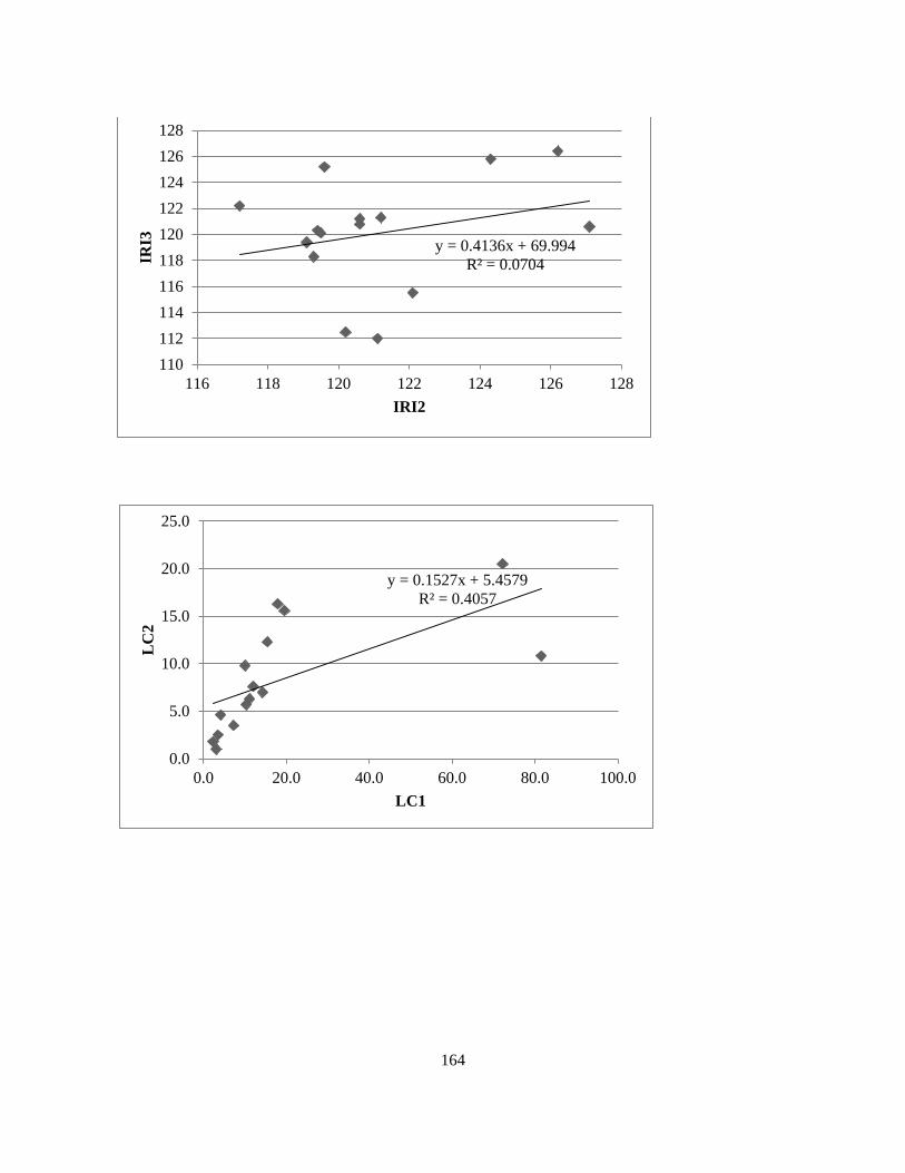
164
y = 0.4136x + 69.994
R² = 0.0704
110
112
114
116
118
120
122
124
126
128
116 118 120 122 124 126 128
IRI3
IRI2
y = 0.1527x + 5.4579
R² = 0.4057
0.0
5.0
10.0
15.0
20.0
25.0
0.0 20.0 40.0 60.0 80.0 100.0
LC
2
LC1

165
y = 0.3029x + 6.181
R² = 0.7495
0
5
10
15
20
25
30
35
0.0 20.0 40.0 60.0 80.0 100.0
LC
3
LC1
y = 1.2992x + 1.0739
R² = 0.7919
0
5
10
15
20
25
30
35
0.0 5.0 10.0 15.0 20.0 25.0
LC
3
LC2

166
y = 0.8889x + 0.0111
R² = 0.7619
0.0
0.1
0.1
0.2
0.2
0.3
0 0.05 0.1 0.15 0.2 0.25
AC
2
AC1
y = x
R² = 1
0.0
0.1
0.1
0.2
0.2
0.3
0 0.05 0.1 0.15 0.2 0.25
AC
3
AC1
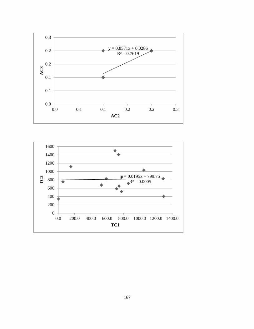
167
y = 0.8571x + 0.0286
R² = 0.7619
0.0
0.1
0.1
0.2
0.2
0.3
0.0 0.1 0.1 0.2 0.2 0.3
AC
3
AC2
y = 0.0195x + 799.75
R² = 0.0005
0
200
400
600
800
1000
1200
1400
1600
0.0 200.0 400.0 600.0 800.0 1000.0 1200.0 1400.0
TC
2
TC1

168
y = -0.1212x + 806.82
R² = 0.0156
0
200
400
600
800
1000
1200
1400
1600
0.0 200.0 400.0 600.0 800.0 1000.0 1200.0 1400.0
TC
3
TC1
y = 0.1252x + 621.88
R² = 0.0124
0
200
400
600
800
1000
1200
1400
1600
0 500 1000 1500 2000
TC
3
TC2

169
y = 0.5682x + 0.0877
R² = 0.8098
0.15
0.17
0.19
0.21
0.23
0.25
0.27
0.29
0.31
0.15 0.20 0.25 0.30 0.35 0.40
AC
R2
ACR1
y = 0.6501x + 0.0718
R² = 0.8126
0.15
0.17
0.19
0.21
0.23
0.25
0.27
0.29
0.31
0.15 0.20 0.25 0.30 0.35 0.40
AC
R3
ACR1

170
y = 1.0386x - 0.0047
R² = 0.8271
0.15
0.17
0.19
0.21
0.23
0.25
0.27
0.29
0.31
0.15 0.17 0.19 0.21 0.23 0.25 0.27 0.29
AC
R3
ACR2
y = 0.5747x + 0.1503
R² = 0.8293
0.29
0.31
0.33
0.35
0.37
0.39
0.41
0.43
0.45
0.30 0.35 0.40 0.45 0.50 0.55
TR
2
TR1

171
y = 0.7407x + 0.0876
R² = 0.8296
0.3
0.32
0.34
0.36
0.38
0.4
0.42
0.44
0.46
0.48
0.30 0.35 0.40 0.45 0.50 0.55
TR
3
TR1
y = 1.1868x - 0.0679
R² = 0.8482
0.3
0.32
0.34
0.36
0.38
0.4
0.42
0.44
0.46
0.30 0.32 0.34 0.36 0.38 0.40 0.42 0.44
TR
3
TR2

172
y = 0.71x + 12.554
R² = 0.482
38.00
40.00
42.00
44.00
46.00
48.00
50.00
37.00 39.00 41.00 43.00 45.00 47.00 49.00
AT
2
AT1
y = 0.6135x + 17.225
R² = 0.4346
37
39
41
43
45
47
49
35.00 37.00 39.00 41.00 43.00 45.00 47.00 49.00
AT
3
AT1

173
y = 0.7215x + 12.701
R² = 0.6286
37
39
41
43
45
47
49
40.00 42.00 44.00 46.00 48.00 50.00
AT
3
AT2
y = 0.0839x + 10.665
R² = 0.0162
8.00
9.00
10.00
11.00
12.00
13.00
14.00
15.00
4.00 6.00 8.00 10.00 12.00 14.00 16.00
AR
2
AR1
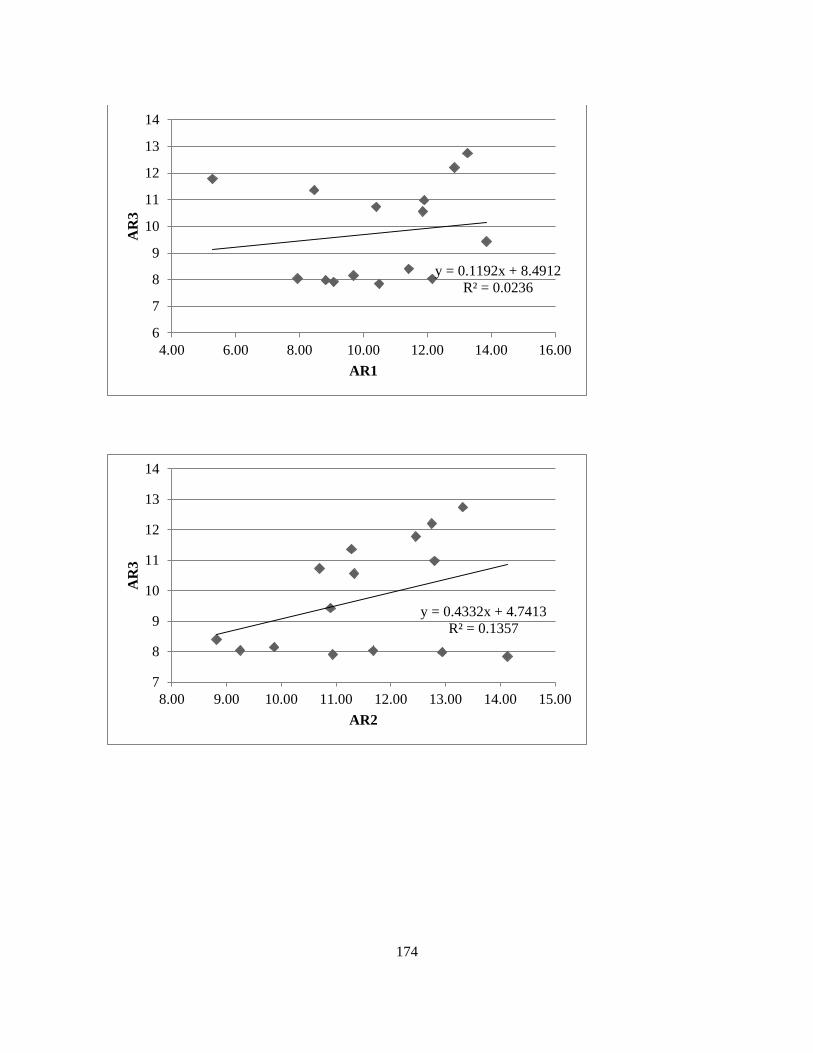
174
y = 0.1192x + 8.4912
R² = 0.0236
6
7
8
9
10
11
12
13
14
4.00 6.00 8.00 10.00 12.00 14.00 16.00
AR
3
AR1
y = 0.4332x + 4.7413
R² = 0.1357
7
8
9
10
11
12
13
14
8.00 9.00 10.00 11.00 12.00 13.00 14.00 15.00
AR
3
AR2

175
y = 0.2715x + 922.82
R² = 0.1415
800.00
900.00
1000.00
1100.00
1200.00
1300.00
1400.00
1500.00
1600.00
1700.00
1800.00
500.00 1000.00 1500.00 2000.00 2500.00 3000.00
FI2
FI1
y = 0.2514x + 927.79
R² = 0.0948
500
700
900
1100
1300
1500
1700
1900
2100
2300
500.00 1000.00 1500.00 2000.00 2500.00 3000.00
FI3
FI1

176
y = 0.6725x + 393.3
R² = 0.3536
700
900
1100
1300
1500
1700
1900
2100
2300
700.00 900.00 1100.00 1300.00 1500.00 1700.00 1900.00
FI3
FI2
y = 0.1128x + 115.33
R² = 0.0134
100
110
120
130
140
150
160
90 100 110 120 130 140 150 160
FT
2
FT1

177
y = -0.3874x + 182.72
R² = 0.1615
110
115
120
125
130
135
140
145
150
155
160
90 100 110 120 130 140 150 160
FT
3
FT1
y = 0.3171x + 93.372
R² = 0.1026
110
115
120
125
130
135
140
145
150
155
160
100 110 120 130 140 150 160
FT
3
FT2