the effect of a large hog barn operation on residential ... · the effect of a large hog barn...

J O S R E u V o l . 6 u N o . 1 – 2 0 1 4

The Ef fec t o f a Large Hog Barn

Operat ion on Res ident ia l Sales

Pr ices in Marshal l County , KY

A u t h o r s Robert A. Simons, Youngme Seo, and Spenser Robinson

A b s t r a c t In this paper, we examine the economic impact of a tightly clusteredcomplex of hog barns, a type of concentrated animal feeding operation(CAFO) on residential property in a rural area near Benton, Kentucky.The operation creates noxious and offensive odors associated withswine-raising and waste disposal activities. Theory and practice indicatethat buyers would avoid purchasing a property believed to becontaminated or subject to effects of unsustainable environmentaldisamenities. Using hedonic regression analysis, the results show pricereductions of 23%–32% for residential properties sold within 1.25 milesof the facility, and much larger losses northeast (downwind) of thefacility.

In this case study, we examine the economic impact of a hog barn, a type ofconcentrated animal feeding operation (CAFO) on residential property. The CAFOfor this case study includes a tightly clustered complex of hog barns, with capacityfor several thousand hogs, which was built and opened in a rural area near thetown of Benton, Kentucky in 2007. After about a full year of operations thatallows the waste pit to fill, the operation created noxious and offensive odorsassociated with swine-raising and waste disposal activities. Theory and practiceindicates that, all else being equal, buyers would avoid purchasing a propertysubject to effects of an environmental disamenity because of unpleasant odors,possible health risks, reduced use, difficulty in reselling the property, uncertainty,and nuisance associated with these environmental issues. Therefore, propertiessuffering from proximity to a hog farm can be expected to sell less frequently andat a discounted price compared with properties not so situated. The amount of thediscount can be equated to the sustainability adjustment to allow the properties totransact in the marketplace.

To determine potential reductions in sales prices, we reviewed the academicliterature regarding the impact of CAFOs on property values; conducted a fieldtrip to the project location and held interviews with affected parties living nearby;reviewed odor logs maintained by residents in the case area at various dates from2007 through 2011, and also reviewed the environmental report of an expert inodor modeling. Next, we built a data set of approximately 270 residential salesand performed a hedonic regression analysis of sales in Marshall County,Kentucky from 2002 through 2012.1

9 4 u S i m o n s , S e o , a n d R o b i n s o n

Our main findings indicate statistically significant reduction of 23%–32% inresidential sales prices due to the presence of the hog barn and its operationswithin a 1.25-mile radius from the hog barn complex. Higher losses are observednortheast of the facility, consistent with wind direction and a comprehensivecompilation of the order logs.

u L i t e r a t u r e

Both economic theory and empirical evidence from peer-reviewed literatureindicate that real property would be negatively affected by environmentaldisamenities, including the repeated presence of noxious or nuisance odors fromnearby commercial activities such as CAFOs, where the existence of such a historyof nuisance odors would need to be disclosed to potential buyers. In a rural area,the local knowledge of potential buyers is also expected to be relatively high,because of the lack of outside interest in living in this relatively isolated area.Identification and quantification of the negative impact of noxious odors canreadily be determined through one or a combination of well-established,scientifically accepted real estate analytical techniques including hedonicregression, real estate sales trends analysis, contingent valuation analysis, and sale-resale analysis, although the preponderance of the literature cited below relies onregression analysis.

Hog farms are a type of CAFO. The other main types of CAFOs include cattleand chicken farms. Smaller operations handle several hundred or a few thousandanimals at a time, and larger ones can grow to 10,000 animals or more. Sometimesthe facilities have a cluster of animal barns. Activities at a CAFO typically includegrowing, but not slaughtering or butchering the animals. The work is relativelyunpleasant, and much of the animal care is automated or handled by immigrantworkers. CAFOs are typically located in relatively isolated areas because ofpotential negative amenities, including some noise, but especially odors. The bulkof the odors usually emanate from concentrated pits of animal by-products, suchas urine, feed, body fluids, feces, medicine, and dead animal parts. These pits arerarely emptied, and a typical pit may be an acre in size and 20 feet deep: a largeone could be three acres and 30 feet deep (Price, 2010). The liquids contained ina hog barn pit can lead to a strong odor, including chemicals such as ammoniaand hydrogen sulfide. Because industrial-sized fans are often used to dissipate theodors locally, direction of fans and wind direction can be a large factor in wherethe odors go, and the impacts they have on nearby property.

In a seminal quantitative study of the impact of CAFOs on proximate propertyvalues, Palmquist, Roka, and Vukina (1997) used hedonic regression to analyze237 arms-length transactions of rural, non-farm residences in nine North Carolinacounties from January 1992 through July 1993. Their analysis, which evaluatedimpact based on the density of swine herds (equivalent to hog farms as we use itin this article) within concentric rings at one-half mile, one mile, and two-milesfrom each house, found a statistically significant reduction in house prices of up

T h e E f f e c t o f a L a r g e H o g B a r n O p e r a t i o n u 9 5

J O S R E u V o l . 6 u N o . 1 – 2 0 1 4

to 9% for each new hog operation opened, with the greatest losses occurring inareas of previously low hog farming density.

In an article outlining the scope of potential value diminution for propertieslocated in the vicinity of CAFOs, Kilpatrick (2001) summarized a University ofMissouri study that found losses to range from 6.6% for vacant land within threemiles of the CAFO to 88% for a home within 0.1 mile of the facility. He alsoreported the results of single-property consulting studies, which found diminutionof 50% for a fruit-and-vegetable family farm located one-quarter mile from aCAFO, 50% for a horse-breeding farm/residence 1,000 feet from a porkprocessing facility, and 60% for a residence 700 feet from another pork processingfacility. In a recent conference paper, the authors also reported newer empiricalstudies consistently showing property losses, including some of the papers citedbelow (Kilpatrick, 2013).

Isakson and Ecker (2008) used hedonic regression to analyze 5,822 single-familyhomes that sold between January 2000 and November 2004 in Black HawkCounty, Iowa, an area which included 39 swine (hog) CAFOs. The studyincorporated a measure of the effects of prevailing winds, concentric circleanalysis around the CAFOs, and spatial correlation factors. Within 2 miles of aCAFO, the authors found losses of 44% for houses directly downwind and 17%for houses at an average oblique wind angle, with wind angle the most powerfulexplanatory variable in their model.

Using hedonic regression, Herriges, Secchi, and Babcock (2005) evaluate 1,145rural, owner-occupied home sales (arms-length transactions) from 1992 to 2002in five Iowa counties with an aggregate of 349 livestock facilities (98% of whichwere swine facilities). The authors found statistically significant property valuereductions of about 15% at one-quarter mile and 9% at one-half mile downwindof a CAFO.

Ready and Abdalla (2005) examined the impact of agricultural land use as bothan amenity and disamenity. The hypothesis was that open space has a positiveimpact on residential property values, while local disamenities, including landfills,high-traffic roads, airport, and large-scale animal production and mushroomproduction, have a negative impact. The study area was Berks County,Pennsylvania. The findings indicated that animal production facilities have asignificant negative impact on the property values of 6.4% within 500 meters and4.1% within 800 meters. Large facilities (greater than 300 AEU2 but less than 600AEU) have less impact on residential property values than medium-sized facilities.

As summarized in Exhibit 1, these studies indicate that it is typical to findresidential property value diminution of 10% to 45%, depending on location withrespect to prevailing wind direction, within two miles of swine CAFOs. Lossescan amount to 50% and more for individual properties located in close proximityto CAFOs. The adverse property value impacts are greatest where swine CAFOsare introduced into areas that did not previously contain high-density hog farmingoperations.


Exhibit 1 u Brief Summary of Literature

Author(s) Year Method Findings

Palmquist, Roka, and Vukina 1997 Hedonic 9% loss

Kilpatrick 2001 Case Study 50–83% within 0.1 mile: 7% 3 miles away

Isakson and Ecker 2008 Hedonic 44% for houses downwind and 17% forthose at an average

Herriges, Secchi, and Babcock 2005 Hedonic 9% at one-half mile downwind

Ready and Abdalla 2005 Hedonic 6.4% within 500 meters and 4.1% within800 meters

Kim and Goldsmith 2009 Spatial Lag Model 10% loss

u S t u d y A r e a a n d S a l e s D a t a

The hog barns analyzed in this study are located in a rural area of MarshallCounty, Kentucky, and nearby Benton, Kentucky. The main complex includes apair of large hog barns. The area’s topography is dominated by level land andslightly rolling hills and a generally warm climate, with mild winters and hothumid summers. The case area (expected to represent the area most affected)where the affected residential properties are located is within a 1.25-mile radiusof the main hog barn complex. All areas outside this radius are considered control(likely unaffected) property. However, since, the empirical evidence citied abovesuggests that the zone of affected property may be larger: in other words, part ofthe control area (outside the affected zone) may also suffer from diminishedproperty values, we also tested an area between 1.25 and 2 miles from the hogfarm complex. The case area and nearby control areas were all in Marshall Countywithin about seven miles of the hog farm complex. They contain similar typesand a similar range of housing stock, and were subject to similar local economicconditions, with the exception of their proximity to the subject hog barns,throughout the study period. Exhibit 2 identifies the general locale.

Study Area Particulars

In 2006, a hog farm complex capable of handling 5,000 hogs was proposed in thepredominantly rural study area near Benton, Kentucky. The facility was openedin mid-2007, and within about a year the urine/catchment pool under the facilitybecame full. Several large fans pointing generally west-northwest move odors andheat away from the facility. According to generally available data in the popularpress, hog barns are associated with noxious chemicals including ammonia andhydrogen sulfide; when inhaled, these chemicals can lead to bronchitis, asthma,nosebleeds, brain damage, and seizures (Price, 2010). An expert report thatdocumented environmental conditions (Winegar, 2013) confirmed the presence ofthese chemicals in proportions large enough to be noticed, and the wind direction,and attributed them to the hog farm. These nuisance odors are consistent with


J O S R E u V o l . 6 u N o . 1 – 2 0 1 4

Exhibit 2 u Study Area: Big Picture and Impacted Area


Exhibit 3 u Nearby Resident Odor Log Analysis: Severe Odor Percentages

Note: This is not a random sample of residents. Residents were involved in litigation against the hog farmoperators.

those described in the peer-reviewed literature cited above. A slightly smaller hogfarm operation, opened in about 2010 by the same owner, is located about 1.5miles northwest of the main hog barns. There has also been a smaller chickenfarm operation about 1/3 mile east of the main hog barns for over 15 years, andthis is considered part of the baseline conditions with respect to odors. Both ofthese are shown in Exhibit 3. The case area includes about 300 residentialproperties, with about a third of the parcels being undeveloped land.

Personal interviews with a non-random sample of nearby residents confirmed thatin about 2009 odors started emanating from the plant, and that they wereintermittently bad to very bad in some directions from the facility (especially tothe northwest), and sometimes noticeable in other directions. The odors persistuntil the present day.

Local Resident Odor Logs

Detailed logs of hog barn odor observations (‘‘odor logs’’) were maintained by14 nearby residents over varying periods of time from July 2007 through August


J O S R E u V o l . 6 u N o . 1 – 2 0 1 4

2011. The authors had no control over who provided these odor logs, and we donot assume this is a random sample. However, the logs do support that odors arestrongest towards the northeast, and thus provide valuable information for modeldesign.

We translated these observations into a common 10-point intensity scale,3 andthen calculated, for each location, an average ‘‘odor intensity level’’ and a ‘‘severe-odor’’ percentage (i.e., the percentage of all of the observations that were rated at7 or higher on the 10-point intensity scale).

We employed a geographic information system to plot the severe odor percentagesat the residents’ homes on a map of the case area, which is shown in Exhibit 3,along with recent sales. The results of this process revealed that the largest clusterof severe odor percentage observations indeed occurred to the northeast of thehog barns. Other relatively high severe odor percentages were found to thenorthwest and southeast of the hog barn site, while the plaintiff odor logs showedless frequent severe odors to the southwest of the barns.

Residential Sales Data Set

The real estate market in this part of Kentucky has been resilient, and has largelyavoided the economic downturn that has affected the rest of the United States.Although there is a mix of housing in the study area, from mobile homes on 1⁄4-acre rural lots to newer mansions on 101 acres, a typical house is a 2,000 sq. ft.ranch or bi-level, 15 years old, on 5–10 acres of land, and located along a ruralroad. Benton (population about 4,400) and Murray (home of Murray StateUniversity with a population of about 18,000) are the nearest towns, whilePaducah, Kentucky and Nashville, Tennessee, TN would provide air links. MineralMounds State Park is about 45 minutes east of the area by car. In short, Bentonis a rural area not convenient to urban life.

Exhibits 4a and 4b show local area housing sales price trends. While the balanceof the U.S. was mired in the great recession due in large part to the foreclosurecrisis, the study area was generally experiencing a continuation of steady growthin sales prices and transaction amounts (note in particular control area price trendsin Exhibit 4b). Case area prices vary widely in some years, due to a small numberof sales.

The initial database used to create the regression data set is a mix of local propertyvaluation data (PVA) and the local multiple listing service (MLS), and includedall (the population of) 305 single-family home sales from both the case and controlareas, which transacted between 2002 and 2012. Based on information in theaccompanying deeds and detailed MLS reports, 12 sales were deleted becausethey did not appear to be ‘‘arm’s length.’’ We also deleted 15 sales that were notable to be properly geocoded, leaving 278 transactions. Because this is a ruralarea, this is a relatively small data set, but represents the vast majority of sales inthe affected area and nearby. Hence, the case and nearby control areas aregenerally comparable, and subject to the same economic trends.

1 0 0 u S i m o n s , S e o , a n d R o b i n s o n

Exhibit 4a u Sales Activity and Average Prices for Case and Control Area: 2002–2012

All Sales Sales in Case Area Sales in Control

Sale Year # of Sales Average Price # of Sales Average Price # of Sales Average Price

2002 26 $88,265 4 $90,875 22 $87,791

2003 23 $89,443 3 $40,200 20 $96,830

2004 25 $96,524 6 $72,083 19 $104,242

2005 30 $90,600 4 $98,725 26 $89,350

2006 24 $115,075 2 $112,700 22 $115,291

2007 27 $100,870 2 $245,000 25 $89,340

2008 19 $110,407 2 $58,750 17 $116,485

2009 18 $119,106 2 $90,400 16 $122,694

2010 21 $93,405 5 $78,040 16 $98,206

2011 24 $132,028 5 $200,800 19 $113,930

2012 34 $115,990 8 $71,500 26 $129,679

Exhibit 4b u Average Sales Price Trends

The real estate public sales dataset was corroborated with MLS records whereavailable, and contained virtually all of the variables required for a regressionanalysis. Continuous variables (unless otherwise noted) included property address(needed for geocoding distance and direction from the source of the odors), saleamount (the dependent variable) and year (a dummy variable), interior squarefootage of the building, porch size, garage/carport spaces, year built, bedrooms,

T h e E f f e c t o f a L a r g e H o g B a r n O p e r a t i o n u 1 0 1

J O S R E u V o l . 6 u N o . 1 – 2 0 1 4

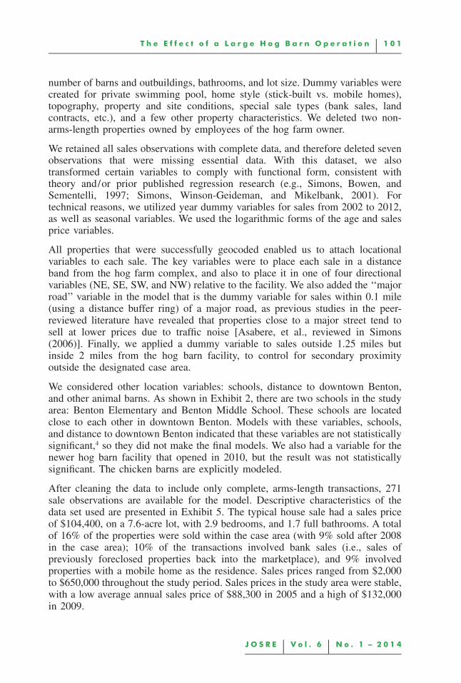
number of barns and outbuildings, bathrooms, and lot size. Dummy variables werecreated for private swimming pool, home style (stick-built vs. mobile homes),topography, property and site conditions, special sale types (bank sales, landcontracts, etc.), and a few other property characteristics. We deleted two non-arms-length properties owned by employees of the hog farm owner.

We retained all sales observations with complete data, and therefore deleted sevenobservations that were missing essential data. With this dataset, we alsotransformed certain variables to comply with functional form, consistent withtheory and/or prior published regression research (e.g., Simons, Bowen, andSementelli, 1997; Simons, Winson-Geideman, and Mikelbank, 2001). Fortechnical reasons, we utilized year dummy variables for sales from 2002 to 2012,as well as seasonal variables. We used the logarithmic forms of the age and salesprice variables.

All properties that were successfully geocoded enabled us to attach locationalvariables to each sale. The key variables were to place each sale in a distanceband from the hog farm complex, and also to place it in one of four directionalvariables (NE, SE, SW, and NW) relative to the facility. We also added the ‘‘majorroad’’ variable in the model that is the dummy variable for sales within 0.1 mile(using a distance buffer ring) of a major road, as previous studies in the peer-reviewed literature have revealed that properties close to a major street tend tosell at lower prices due to traffic noise [Asabere, et al., reviewed in Simons(2006)]. Finally, we applied a dummy variable to sales outside 1.25 miles butinside 2 miles from the hog barn facility, to control for secondary proximityoutside the designated case area.

We considered other location variables: schools, distance to downtown Benton,and other animal barns. As shown in Exhibit 2, there are two schools in the studyarea: Benton Elementary and Benton Middle School. These schools are locatedclose to each other in downtown Benton. Models with these variables, schools,and distance to downtown Benton indicated that these variables are not statisticallysignificant,4 so they did not make the final models. We also had a variable for thenewer hog barn facility that opened in 2010, but the result was not statisticallysignificant. The chicken barns are explicitly modeled.

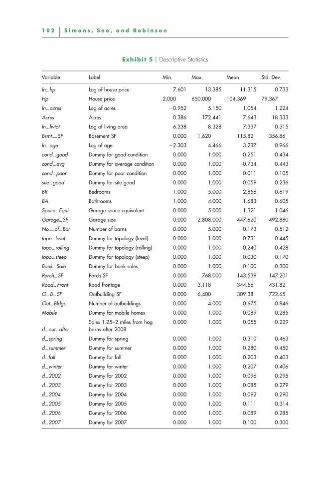
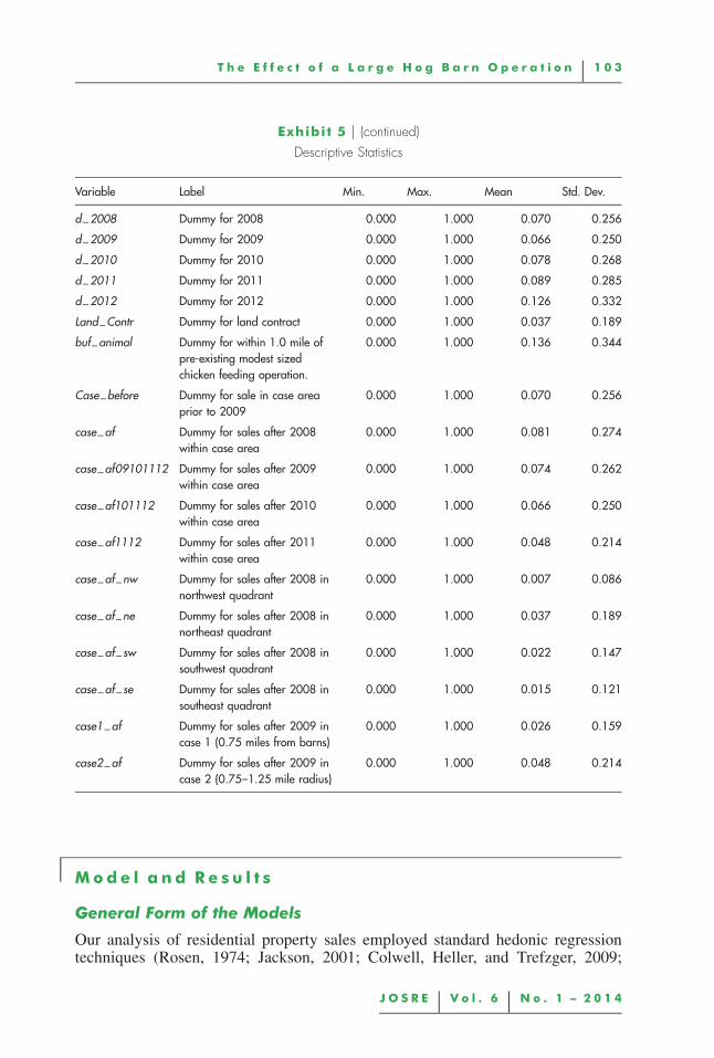
After cleaning the data to include only complete, arms-length transactions, 271sale observations are available for the model. Descriptive characteristics of thedata set used are presented in Exhibit 5. The typical house sale had a sales priceof $104,400, on a 7.6-acre lot, with 2.9 bedrooms, and 1.7 full bathrooms. A totalof 16% of the properties were sold within the case area (with 9% sold after 2008in the case area); 10% of the transactions involved bank sales (i.e., sales ofpreviously foreclosed properties back into the marketplace), and 9% involvedproperties with a mobile home as the residence. Sales prices ranged from $2,000to $650,000 throughout the study period. Sales prices in the study area were stable,with a low average annual sales price of $88,300 in 2005 and a high of $132,000in 2009.


Exhibit 5 u Descriptive Statistics

Variable Label Min. Max. Mean Std. Dev.

ln hp Log of house price 7.601 13.385 11.315 0.733

Hp House price 2,000 650,000 104,369 79,367

ln acres Log of acres 20.952 5.150 1.054 1.224

Acres Acres 0.386 172.441 7.643 18.333

ln livtot Log of living area 6.238 8.328 7.337 0.315

Bsmt SF Basement SF 0.000 1,620 115.82 356.86

ln age Log of age 22.303 4.466 3.237 0.966

cond good Dummy for good condition 0.000 1.000 0.251 0.434

cond avg Dummy for average condition 0.000 1.000 0.734 0.443

cond poor Dummy for poor condition 0.000 1.000 0.011 0.105

site good Dummy for site good 0.000 1.000 0.059 0.236

BR Bedrooms 1.000 5.000 2.856 0.619

BA Bathrooms 1.000 4.000 1.683 0.605

Space Equi Garage space equivalent 0.000 5.000 1.321 1.046

Garage SF Garage size 0.000 2,808.000 447.620 492.880

No of Bar Number of barns 0.000 5.000 0.173 0.512

topo level Dummy for topology (level) 0.000 1.000 0.731 0.445

topo rolling Dummy for topology (rolling) 0.000 1.000 0.240 0.428

topo steep Dummy for topology (steep) 0.000 1.000 0.030 0.170

Bank Sale Dummy for bank sales 0.000 1.000 0.100 0.300

Porch SF Porch SF 0.000 768.000 143.539 147.201

Road Front Road frontage 0.000 3,118 344.56 431.82

O B SF Outbuilding SF 0.000 6,400 309.38 722.65

Out Bldgs Number of outbuildings 0.000 4.000 0.675 0.846

Mobile Dummy for mobile homes 0.000 1.000 0.089 0.285

d out afterSales 1.25–2 miles from hogbarns after 2008

0.000 1.000 0.055 0.229

d spring Dummy for spring 0.000 1.000 0.310 0.463

d summer Dummy for summer 0.000 1.000 0.280 0.450

d fall Dummy for fall 0.000 1.000 0.203 0.403

d winter Dummy for winter 0.000 1.000 0.207 0.406

d 2002 Dummy for 2002 0.000 1.000 0.096 0.295

d 2003 Dummy for 2003 0.000 1.000 0.085 0.279

d 2004 Dummy for 2004 0.000 1.000 0.092 0.290

d 2005 Dummy for 2005 0.000 1.000 0.111 0.314

d 2006 Dummy for 2006 0.000 1.000 0.089 0.285

d 2007 Dummy for 2007 0.000 1.000 0.100 0.300


J O S R E u V o l . 6 u N o . 1 – 2 0 1 4

Exhibit 5 u (continued)

Descriptive Statistics

Variable Label Min. Max. Mean Std. Dev.

d 2008 Dummy for 2008 0.000 1.000 0.070 0.256

d 2009 Dummy for 2009 0.000 1.000 0.066 0.250

d 2010 Dummy for 2010 0.000 1.000 0.078 0.268

d 2011 Dummy for 2011 0.000 1.000 0.089 0.285

d 2012 Dummy for 2012 0.000 1.000 0.126 0.332

Land Contr Dummy for land contract 0.000 1.000 0.037 0.189

buf animal Dummy for within 1.0 mile ofpre-existing modest sizedchicken feeding operation.

0.000 1.000 0.136 0.344

Case before Dummy for sale in case areaprior to 2009

0.000 1.000 0.070 0.256

case af Dummy for sales after 2008within case area

0.000 1.000 0.081 0.274

case af09101112 Dummy for sales after 2009within case area

0.000 1.000 0.074 0.262


0.000 1.000 0.066 0.250


0.000 1.000 0.048 0.214

case af nw Dummy for sales after 2008 innorthwest quadrant

0.000 1.000 0.007 0.086

case af ne Dummy for sales after 2008 innortheast quadrant

0.000 1.000 0.037 0.189

case af sw Dummy for sales after 2008 insouthwest quadrant

0.000 1.000 0.022 0.147

case af se Dummy for sales after 2008 insoutheast quadrant

0.000 1.000 0.015 0.121

case1 af Dummy for sales after 2009 incase 1 (0.75 miles from barns)

0.000 1.000 0.026 0.159

case2 af Dummy for sales after 2009 incase 2 (0.75–1.25 mile radius)

0.000 1.000 0.048 0.214

u M o d e l a n d R e s u l t s

General Form of the Models

Our analysis of residential property sales employed standard hedonic regressiontechniques (Rosen, 1974; Jackson, 2001; Colwell, Heller, and Trefzger, 2009;


Simons, Bowen, and Sementelli, 1997; Simons, Winson-Geideman, andMikelbank, 2001; and Seo and Simons, 2012). The dependent variable is the logof housing sales prices. The independent variables include a number of controlvariables, plus one that isolates the effect odors (Eq. 1). We hypothesize that, afterthe opening of the hog barns, homes within a 1.25-mile radius of the facility havesold at lower prices than those in the control area.

To check for spatial autocorrelation in housing sales prices (Kim and Goldsmith,2009), we used the Lagrange Multiplier (LM) test for lag, for error, RobustLagfor lag, and RobustLM for error. None of the test results indicated spatialautocorrelation was a concern.5

Two models plus an examination of the effects of the hog farm over time arepresented: a baseline model including all sales in the case area from 2009 onward;a space model focusing on wind direction; and a series of interactive models overtime and space that allows us to identify variations in price impact over varyingtime periods, based on a case property’s direction from the hog barn complex. Allmodels are generally specified as follows:

Ln HP 5 b0 1 b1HC 1 b2LOC 1 b3TIME

1 b4CASE AF 1 «, (1)

where:

Ln HP 5 The (log of the) sale price of each home that sold in our dataset;b0 5 The model intercept;

HC 5 A matrix of physical housing characteristics;LOC 5 A matrix of dummy variables for sales within 0.1 mile of a major

road, outside the case area;TIME 5 A matrix of year and season dummy variables;

CASE AF 5 The effect on sales price of location within the case area after thehog barns became fully operative, which can take different formsas discussed below; and

« 5 The error term.

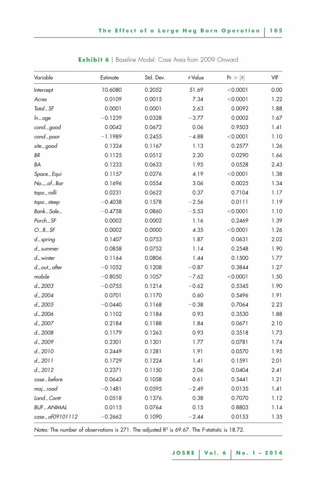
Results: Baseline Model

The results from our baseline model are presented in Exhibit 6. We checked formulticollinearity, and the VIF statistics shown in the far right-hand column arelow, outside the concern of generally accepted cutoffs. We also tested fornormality and heterogeneity using the Kolmogorov-Smirnov test, which indicatedthat there is no normality problem with the dataset. The value of K-S D is 0.07,which is statistically significant at the 99% confidence interval. Similarly,application of the Breusch-Pagan test found no heteroscedasticity.6

The model’s adjusted R2 value at 69.67 is satisfactory, indicating that the variablesused in the model explain about 70% of the variation in sales price. Likewise the


J O S R E u V o l . 6 u N o . 1 – 2 0 1 4

Exhibit 6 u Baseline Model: Case Area from 2009 Onward

Variable Estimate Std. Dev. t-Value Pr . ut u VIF

Intercept 10.6080 0.2052 51.69 ,0.0001 0.00

Acres 0.0109 0.0015 7.34 ,0.0001 1.22

Total SF 0.0001 0.0001 2.63 0.0092 1.88

ln age 20.1239 0.0328 23.77 0.0002 1.67

cond good 0.0042 0.0672 0.06 0.9503 1.41

cond poor 21.1989 0.2455 24.88 ,0.0001 1.10

site good 0.1324 0.1167 1.13 0.2577 1.26

BR 0.1125 0.0512 2.20 0.0290 1.66

BA 0.1233 0.0633 1.95 0.0528 2.43

Space Equi 0.1157 0.0276 4.19 ,0.0001 1.38

No of Bar 0.1696 0.0554 3.06 0.0025 1.34

topo rolli 0.0231 0.0622 0.37 0.7104 1.17

topo steep 20.4038 0.1578 22.56 0.0111 1.19

Bank Sale 20.4758 0.0860 25.53 ,0.0001 1.10

Porch SF 0.0002 0.0002 1.16 0.2469 1.39

O B SF 0.0002 0.0000 4.35 ,0.0001 1.26

d spring 0.1407 0.0753 1.87 0.0631 2.02

d summer 0.0858 0.0752 1.14 0.2548 1.90

d winter 0.1164 0.0806 1.44 0.1500 1.77

d out after 20.1052 0.1208 20.87 0.3844 1.27

mobile 20.8050 0.1057 27.62 ,0.0001 1.50

d 2003 20.0755 0.1214 20.62 0.5345 1.90

d 2004 0.0701 0.1170 0.60 0.5496 1.91

d 2005 20.0440 0.1168 20.38 0.7064 2.23

d 2006 0.1102 0.1184 0.93 0.3530 1.88

d 2007 0.2184 0.1188 1.84 0.0671 2.10

d 2008 0.1179 0.1263 0.93 0.3518 1.73

d 2009 0.2301 0.1301 1.77 0.0781 1.74

d 2010 0.2449 0.1281 1.91 0.0570 1.95

d 2011 0.1729 0.1224 1.41 0.1591 2.01

d 2012 0.2371 0.1150 2.06 0.0404 2.41

case before 0.0643 0.1058 0.61 0.5441 1.21

maj road 20.1481 0.0595 22.49 0.0135 1.41

Land Contr 0.0518 0.1376 0.38 0.7070 1.12

BUF ANIMAL 0.0115 0.0764 0.15 0.8803 1.14

case af09101112 20.2662 0.1090 22.44 0.0153 1.35

Notes: The number of observations is 271. The adjusted R2 is 69.67. The F-statistic is 18.72.


F-statistic is 18.72, satisfactory but consistent with statistical analysis with alimited number of sales.

The coefficients on the housing characteristic control variables are generally asexpected by theory, at over a 90% level of confidence. The variables for lot size,porch size, square footage of living area, number of bedrooms, and number ofbaths have the expected positive signs and possess significantly high t-values.Housing and site condition dummy variables are as expected and statisticallysignificant. Bank sales (20.48) show the expected negative and statisticallysignificant effect on sales prices, as does the mobile home variable (20.81). Thelocational variable (major road) shows the predicted negative effect and isstatistically significant. We used the year 2002 as the base year; the coefficientsfor sales in the years 2003 and 2005 have negative signs but are not statisticallysignificant; the coefficients for sales in the years 2007, 2009, 2010, and 2012reflect statistically significant differences from the base year in the order of a 20%increase, stable since 2007, which is contrary to the national trend of a downwardcycle, consistent with the figures in Exhibit 4.

We include the variable case before, which covers the subject area prior to theCAFO beginning operations. The coefficient is insignificant from zero, showingthat prior to the CAFO, the subject area prices moved similarly to the surroundingareas, ceteris paribus.

We initially employed the commonly-used distance-rings approach in the hedonicmodel to estimate the effect of location within the case area.7 Using the 1.25-miledistance ring, we identified sales in the case area from 2009 onward; the coefficientfor the corresponding variable (case af09101112) shows a coefficient of 20.27,or an estimated loss of 23%8 (Halvorsen and Palmquist, 1980) after performinglog transformation, and this figure is statistically significant at a level of morethan 95%. In other words, this baseline regression model reveals that the marginaleffect of a home’s location within the case area (i.e., within a 1.25-mile radius ofthe subject hog barns after December 31, 2008, there is a 23% reduction in salesprice, holding all other factors constant).9

Space Model Results: Direction and Time within Case Area

As noted above, the analysis of odor observation logs kept by a non-randomsample of nearby residents at varying times from 2007 through 2011 demonstratedthat hog barn odors appeared to be somewhat stronger and more prevalent atlocations to the north and northeast of the hog barns than in other portions of thecase area. As per Winegar (2013), prevailing winds in southwestern MarshallCounty tend to blow more often and with greater intensity from south andsouthwest of the hog barn complex. Accordingly, in our space model we exploredthe marginal effect on sales price of a home’s location within the four cardinalwind directions from the hog farm facility. The case area is split into fourdirections, with the reference category defined as outside in the case area. Thesample sizes are limited, but there is particular interest in the northeast quadrantof the case area (i.e., at headings between 08 (north) and 908 (east) from the hog


J O S R E u V o l . 6 u N o . 1 – 2 0 1 4

barns), during the period beginning January 1, 2009. The corresponding variableis case af0912 ne. The results of the regression model are presented in Exhibit7.

The adjusted R2 value and F-statistic in the space model are slightly higher thanthose in the baseline model, at 71.54 (indicating that the space model explainsabout 72% of the variation in sales price among all sales in the dataset) and 18.86,respectively. The signs of the variable coefficients in this hedonic regression modelare similar to those in the baseline model. The coefficient of the interactivevariable (case af0912 ne) is statistically significant (at a level greater than 99%)and negative, indicating that the marginal effect of a property’s location withinthe northeast quadrant of the case area, after December 31, 2008, is a reductionin sales price of 49%,10 holding all other factors constant. This clearly shows thatfor these data, properties located northeast of the hog barns have sustained larger-than-average losses.

However, due to the relatively small number of sales (the number of sales in thisNE quadrant is 13), caution is advised in putting too much weight on themagnitude of the parameter estimate, which seems quite large. Also, the otherwind quadrants had only a handful of sales or less, and none of their parameterestimates were statistically significant. Hence, prudence indicates that we can onlysay that wind direction matters.

Alternative Runs Over Time and Space

In this sensitivity analysis, we explored a number of additional variations,including varying start time of the effects, and splitting distance rings within thecase area. For start time, we varied the starting year, going from 2008 when thestench pit was filling up, to 2009 and 2010, through 2012 in all cases. It’simportant to watch the number of sales dwindling: the strongest results are whenthe model contains at least 15 sales.

We also took a closer look at distance rings. We attempted three rings: within0.75 miles of the hog barns, 0.75–1.25 miles, and 1.25–2.0 miles. We ran intosample size issues again: the 0.75–1.25 miles from hog barns (referred to as case2)had over 15 sales, enough to report, and the losses there were higher than averagefor the entire case area.11 The close-in ring did not have enough sales to findsignificant results. Exhibits 6 and 7 do not show a statistically significant effectoutside the 1.25-mile range. However, there were only 15 sales, which is a smallnumber for statistical reliability in these models.

We also conducted several additional model runs with five outliers (high and lowsales prices) removed. Results continued to show significant reductions onproperty sales prices after 2009, about 15% lower than the full model. The spacemodel still had significant higher losses northeast of the hog farms, but at amagnitude 25%–30% lower than the baseline model. Thus the model appears tohave potentially influential outliers, but caution is again advised because thenumber of sales is smaller still. It can be concluded that the magnitude of themain results vary somewhat but not their statistical significance.


Exhibit 7 u Space Model Case Area (Northeast Quadrant) from 2009 Onward


Intercept 10.5958 0.1989 53.28 ,0.0001 0.00

Acres 0.0107 0.0014 7.43 ,0.0001 1.23

Total SF 0.0001 0.0000 2.22 0.0271 1.91

ln age 20.1249 0.0319 23.92 0.0001 1.68

cond good 0.0192 0.0654 0.29 0.7688 1.42

cond poor 21.1710 0.2379 24.92 ,0.0001 1.10

site good 0.1375 0.1131 1.22 0.2252 1.26

BR 0.1179 0.0497 2.37 0.0185 1.67

BA 0.1382 0.0613 2.25 0.0252 2.43

Space Equi 0.1127 0.0269 4.19 ,0.0001 1.40

No of Bar 0.2103 0.0546 3.85 0.0002 1.38

topo rolli 0.0392 0.0604 0.65 0.5168 1.18

topo steep 20.4251 0.1532 22.78 0.0060 1.19

Bank Sale 20.4764 0.0832 25.73 ,0.0001 1.10

Porch SF 0.0002 0.0002 1.27 0.2046 1.39

O B SF 0.0002 0.0000 5.12 ,0.0001 1.30

d spring 0.1198 0.0732 1.64 0.1032 2.03

d summer 0.0753 0.0731 1.03 0.3037 1.91

d winter 0.1030 0.0784 1.31 0.1899 1.78

d out after 20.1367 0.1172 21.17 0.2446 1.27

mobile 20.7621 0.1029 27.40 ,0.0001 1.52

d 2003 20.0737 0.1176 20.63 0.5315 1.90

d 2004 0.0722 0.1134 0.64 0.5247 1.91

d 2005 20.0558 0.1132 20.49 0.6224 2.24

d 2006 0.1033 0.1148 0.90 0.3691 1.89

d 2007 0.2098 0.1151 1.82 0.0696 2.11

d 2008 0.1362 0.1233 1.10 0.2704 1.76

d 2009 0.1860 0.1269 1.47 0.1441 1.77

d 2010 0.3172 0.1258 2.52 0.0123 2.00

d 2011 0.1001 0.1194 0.84 0.4028 2.04

d 2012 0.2247 0.1115 2.02 0.0450 2.42

case before 0.0607 0.1026 0.59 0.5544 1.22

maj road 20.1317 0.0588 22.24 0.0259 1.47

Land Contr 0.1613 0.1353 1.19 0.2346 1.15

BUF ANIMAL 0.0201 0.0746 0.27 0.7877 1.16


J O S R E u V o l . 6 u N o . 1 – 2 0 1 4

Exhibit 7 u (continued)

Space Model Case Area (Northeast Quadrant) from 2009 Onward


class af ne 20.6782 0.1476 24.60 ,0.0001 1.37

class af nw 20.1167 0.2919 20.40 0.6898 1.11

class af se 0.1540 0.2103 0.73 0.4648 1.14

class af sw 0.2270 0.1722 1.32 0.1886 1.14

Notes: The number of observations is 271. The adjusted R2 is 71.54. The F-statistic is 18.86.

Exhibit 8 u Compilation of Several Alternative Runs

ModelCase Area2008–2012

Case Area2009–2012

Case Area2010–2012

Case Area2009–2012NE of Hogs

Case Area2009–2012NE of Hogs

Case 22009–20120.75–1.25 miles

Parameter Est. 20.20 20.27 20.32 20.68 20.78 20.56

T-stat. 21.94 22.47 22.76 24.60 25.13 24.09

Model Adj. R 2 69.52 69.81 70.00 71.54 72.11 71.04

# of Sales 22 20 18 10 9 17

u C o n c l u s i o n

Hog farms are generally associated with a reduction in nearby residential salesprices, and our results support this expectation. Our hedonic regression analysisfound a statistically significant average reduction in property value averagingalmost 23% across the subject area within 1.25 miles of the facility for salestransacting from 2009 through 2012, holding other factors constant. Results fromour regression models indicate that this negative impact on affected area propertyvalues is increasing, as the regression analysis disclosed an average property valuediminution of 27% for sales from 2010 onward. We also found a substantiallyhigher diminution in value for properties located in the northeast quadrant of thesubject area, which suffer from the most prominent prevailing winds in the area.The discount allows properties that otherwise would not sell to be transacted inthe market place, and thus represents a ‘‘sustainability adjustment.’’

The peer-reviewed professional literature reports that it is not unusual to findproperty value losses of 10% to 45% within 2 miles of CAFOs, with the effectsbeing largest and most pronounced downwind of the facilities and in areas thatdo not already have high densities of existing CAFOs. The subject area fits thislatter category, as the subject hog barns and a smaller, related facility are the first


swine CAFOs to be established in Marshall County. The peer-reviewed literaturealso contains examples of property value losses in the range of 50% to 60% forindividual homes in close proximity to CAFOs, with higher-valued propertiessustaining particularly large percentage losses in value. Our results match closelywith Isakson and Ecker’s (2008) findings concerning the magnitude of losses andimportance of wind direction.

With respect to time effects, we found increased impacts over time, with limitedeffects in the transitional year when the swill pits on the hog farms were fillingup and increasing over the next several years. We conclude that wind direction ismore important than pure distance in determining the magnitude of the effects onresidential property values, but qualify this with our limited number of sales.

u E n d n o t e s

1 The senior author was retained as an expert witness by the plaintiffs in a legal caserelated to this study in 2013.

2 AEU is animal equivalent unit.3 Many of the residents’ observations were recorded on such a 10-point scale of odor

intensity, but others were in the form of verbal descriptions.4 The t-value is 20.53 for the distance to downtown Benton variable, and R-squared is

slightly lower than the model without this variable.5 Spatial results were: 0.09 (0.764) for LM lag, 0.09 (0.760) for LM error, 0.43 (0.513)

for Robustlag, and 0.43 (0.512) for Robust LM error, respectively. The numbers inparentheses are the p-values. All results are below threshold levels.

6 We also examined the dataset for heteroscedasticity by visual inspection of a scatterplotof sale price and model residuals, and no fanning pattern was evident.

7 Simons and Seo (2011) found a positive externality of a religious facility campus onneighboring housing sale prices. They used hedonic regression analysis using 2,500 salesin Ohio, and identified sales within quarter-mile distance buffers. A similar distance ringapproach was taken by Smolen et al., Reichert, and Nelson in their analyses of thenegative amenity from proximity to landfills [in Simons (2006, p. 96)].

8 Percentage log transformation of dummy variables, [(e0.2662) 2 1] * 100 5 23%.9 As additional interpretive context for this result, note that the coefficient for the variable

case before is positive but not statistically significant. In other words, over the timeperiod before the odors became apparent covered by the dataset (i.e., 2002–2007), thesales data do not allow us to conclude that the marginal effect on sales price of locationwithin the ‘‘future’’ area that would be affected by odors was other than zero. Thus, thesales performance of homes within the case area did not significantly differ from homesthroughout the entire study area. That is, the observed diminution in value of case areahomes after 2009 represents a genuine and abrupt change in their sales performancerelative to a multi-year pre-existing pattern in which such homes statistically matchedthe sales performance of homes in the surrounding areas of southwestern MarshallCounty.

10 Percentage log transformation of dummy variables, [(e0.6782) 2 1] * 100 5 49%.11 In the outlier-free models reported just below, case2 had significant losses equivalent to

the entire case area: hence no model shows closer-in sales with higher losses.


J O S R E u V o l . 6 u N o . 1 – 2 0 1 4

u R e f e r e n c e s

Colwell, P., J. Heller, and J. Trefzger. Expert Testimony: Regression Analysis and OtherSystematic Methodologies. The Appraisal Journal, 2009, Summer, 253–62.

Halvorsen, R. and R. Palmquist. The Interpretation of Dummy Variables in SemilogarithmicEquations. American Economic Review, 1980, 70, 474–75.

Herriges, J., S. Secchi, and B.A. Babcock. Living with Hogs In Iowa: The Impact ofLivestock Facilities on Rural Residential Property Values. Land Economics, 2005, 81:4,530–45.

Isakson, H.R. and M.D. Ecker. An Analysis of the Impact of Swine CAFOs on the Valueof Nearby Houses. Agricultural Economics, 2008, 39:3, 365–72.

Jackson, T. Evaluating Environmental Stigma with Multiple Regression Analysis. TheAppraisal Journal, 2001, Fall, 363–69.

Kilpatrick, J.A. Concentrated Animal Feeding Operations and Proximate Property Values.The Appraisal Journal, 2001, July, 301–06.

Kilpatrick, J.A. Appraisal Implications of Proximity to Feedlots. Paper presented at theARES Annual Meeting, Hawaii, April 2013.

Kim, J. and P. Goldsmith. A Spatial Hedonic Approach to Assess the Impact of SwineProduction on Residential Property Values. Environmental and Resource Economics, 2009,42:4, 509–34.

Palmquist, R.B., F.M. Roka, and T. Vukina. Hog Operations, Environmental Effects, andResidential Property Values. Land Economics, 1997, 73:1, 114–24.

Price, C. 101 Places Not to See before You Die. New York, NY: HarperCollins Publishers,2010.

Ready, R.C. and C.W. Abdalla. The Amenity and Disamenity Impacts of Agriculture:Estimates from a Hedonic Pricing Model. American Journal of Agricultural Economics,2005, 87:2, 314–26.

Rosen, S. Hedonic Prices and Implicit Markets: Product Differentiation in PureCompetition. Journal of Political Economy, 1974, 82:1, 34–55.

Seo, Y. and R.A. Simons. Residential Value Halos: The Effect of a Jewish OrthodoxCampus On Residential Property Values. 2011 International Real Estate Review.

Simons, R.A. When Bad Things Happen to Good Property. Washington DC: EnvironmentalLaw Institute Press (released 2006).

Simons, R.A., W. Bowen, and A. Sementelli. The Effect of Underground Storage Tankson Residential Property Values in Cuyahoga County, Ohio. Journal of Real Estate Research,1997, 14:1/2, 29–42.

Simons, R.A., K. Winson-Geideman, and B. Mikelbank. The Effects of an Oil PipelineRupture on Single-Family House Prices. The Appraisal Journal, 2001, 69, 410–18.

Winegar, E. Air Modeling Expert Report on Marshall County, KY Hog Farm Case. 2013.

Robert A. Simons, Cleveland State University, Cleveland, OH 44115 [email protected].

Youngme Seo, [email protected].

Spenser Robinson, Central Michigan University, Mt. Pleasant, MI 48859 [email protected].

This page intentionally left blank

the effect of a large hog barn operation on residential ... · the effect of a large hog barn...

Documents