The Economics of CO2 Sequestration through Enhanced Oil Recovery

Klaas van ’t Veld,* Charles F. Mason∗, and Andrew Leach**

Abstract

In this paper, we provide an overview of the economics of CO2-enhanced oil recovery (EOR), considering the

influence of climate-change policy on optimal management of CO2-EOR projects. EOR is a significant and

rapidly growing portion of oil production in the US. This is an important development for climate-change

policy as most of the injected CO2 remains underground after fields are decommissioned. If the injected CO2

comes from anthropogenic sources, EOR therefore constitutes a form of carbon capture and sequestration.

The potential magnitude of this sequestration potential is substantial; recent estimates indicate EOR has the

potential to sequester emissions from more than 90 one-gigawatt-size coal-fired power plants for 30 years. In

addition, these projects generate revenues from the incremental oil that they recover. While EOR projects

currently treat CO2 as a costly input, operators may receive carbon credits, tax credits, or other types of

subsidies for any CO2 they sequester in the context of climate-change policy. Because these subsidies then

become a new source of revenues, additional to revenues from oil, the question arises how operators should

“co-optimize” oil recovery and CO2 sequestration.

*Department of Economics & Finance, University of Wyoming, 1000 E. University Ave., Laramie, WY 82071.E-mail: klaas@uwyo.edu, bambuzlr@uwyo.edu**University of Alberta School of Business, 3-40K Business Building, Edmonton, Alberta, Canada T6G 2R6.E-mail: andrew.leach@ualberta.ca

2

1. Introduction

The process of injecting CO2 into mature oil fields to increase oil production, referred to as CO2-

enhanced oil recovery (CO2-EOR), contributes a significant and rapidly growing portion of oil

production in the US. According to the most recent biannual survey of EOR production by the Oil

and Gas Journal (Koottungal, 2012), CO2-EOR projects now produce about 350,000 barrels/day

(5.6% of total US oil production), compared to just 190,000 barrels/day (3.2%) in the year 2000.

This is an important development for climate-change policy, because almost all of the injected

CO2 remains underground after fields are decommissioned. Provided therefore that the CO2 comes

from anthropogenic sources, EOR constitutes a form of carbon capture and sequestration (CCS).

Moreover, whereas projects that inject CO2 into saline aquifers incur only costs, EOR projects

generate revenues from the incremental oil that they recover. Recognizing perhaps the political

advantage in emphasizing that captured CO2 can generate economic value, the US Department of

Energy (DOE) has in fact recently “re-branded” CCS to CCUS—the “U” standing for “utiliza-

tion,” mostly in CO2-EOR projects (Marshall, 2012). The DOE’s most recent report on CO2-EOR

(Kuuskraa et al., 2010) dramatizes the sequestration potential of CO2-EOR projects by estimating

that they could collectively sequester the emissions from as many as 93 one-GW-size coal-fired

power-plants for 30 years. In addition, it has widely been argued that promoting CO2-EOR may

provide a “bridge” to widespread capture of CO2 for storage in aquifers (which have far greater

sequestration capacity), by helping pay for required infrastructure.1

In this paper, we provide an overview of the economics of CO2-EOR. Our focus thereby is on

insights from economic analysis that engineering studies have tended to overlook.

We first consider how climate-change policy may influence optimal management of CO2-EOR

projects. Currently, these projects treat CO2 as a costly input, the use of which should be min-

imized. In the context of climate-change policy, however, operators may receive carbon credits,

tax credits, or other types of subsidies for any CO2 they sequester. Because these subsidies then

become a new source of revenues, additional to revenues from oil, the question arises how operators

should “co-optimize” oil recovery and CO2 sequestration.

1 See, e.g., ARI (2010); MIT (2010); Steelman and Tonachel (2010), but see also Dooley et al. (2010) for a dissentingview.

3

q injwat qinjCO2

↓↓

qprdoil

→

↑

qrecCO2 ←← CO2recycling

plant

qseqCO2

qpurCO2

x

x

Figure 1. Schematic of fluid flows in a CO2-EOR project.

2. Modeling Oil Production

Several engineering studies (Asghari and Al-Dliwe, 2004; Jessen et al., 2005a; Kovscek and Cakici,

2005; Babadagli, 2006; Forooghi et al., 2009; Pamukcu and Gumrah, 2009; Ghomian et al., 2010;

Jahangiri and Zhang, 2011) have addressed this question of co-optimization, examining how oper-

ators might modify well-completion, -spacing, and -control decisions, as well as the sequencing of

CO2 and water injection. The usefulness of these studies is limited, however, by the ad hoc criterion

used to compare these decisions: the operator is usually assumed to maximize a simple weighted

sum of cumulative oil recovery and cumulative CO2 sequestration. More realistically, operators

will maximize the net present value (NPV) of project profits—discounted oil and sequestration rev-

enues less operating and investment costs—which we find may result in quite different management

decisions.

One such difference is that, whereas engineering studies tend to hold CO2 injection constant,

NPV maximization dictates a gradually declining CO2-injection rate, to save on CO2 recycling

costs. To see why, consider the schematic of a CO2-EOR flood shown in Figure 1.

On the left, water and compressed CO2 are injected into the reservoir (q injwat and q injCO2), usually

in alternating slugs—a process referred to as “water alternating gas” (WAG) injection. Inside the

reservoir, the injected fluids help move oil towards production wells. In the process of doing so,

some fraction of the injected CO2 remains sequestered in the reservoir (qseqCO2), taking up pore space

vacated by the oil, as does some fraction of the injected water. On the right, a mixture of CO2,

oil, and water flows out of production wells and is separated at the surface into flows of oil (qprdoil ),

recycled and recompressed CO2 (qrecCO2) and recycled water. In order to maintain a given injection

4

ratio of water and CO2, the recycled flows are supplemented with new water and new, purchased

CO2 (qpurCO2).

These physical flows give rise to the following profit flow from an EOR project in a given period

(a year, say):

profit = poilqprdoil︸ ︷︷ ︸

oilrevenues

+ sCO2qseqCO2︸ ︷︷ ︸

CO2

sequestrationsubsidies

− pCO2qseqCO2︸ ︷︷ ︸

CO2

purchasecosts

− crecqrecCO2︸ ︷︷ ︸CO2

recyclingcosts

− coth︸︷︷︸othercosts

, (1)

where poil and pCO2 represent the unit prices of oil and CO2 in the given period, sCO2 any unit

subsidy for CO2 sequestration, crec the unit cost of CO2 recycling (which is a major flow expense

of any EOR project), and finally coth other operating costs (overhead, labor, maintenance, etc.).

For our economic analysis, it is useful to rearrange this profit expression, using two identities

that follow from the schematic of Figure 1.

First, the schematic shows that if a given CO2 injection flow is to be maintained, CO2 purchases

must make up for CO2 sequestration, so qpurCO2= qseqCO2

. Using this identity, we can merge the CO2

sequestration subsidies term sCO2qseqCO2

and the CO2 purchase costs term pCO2qpurCO2

into a single

term (sCO2 − pCO2)qseqCO2. That is, we subtract from the subsidy sCO2 for each unit sequestered the

price pCO2 of the additional unit of CO2 that will have to be purchased in order to make up for

the sequestration and maintain the CO2 injection flow: this price is in effect an indirect cost of

sequestration.

Second, the schematic shows that the quantity of CO2 recycled is just the quantity injected less

that sequestered, so qrecCO2= q injCO2

− qseqCO2. Using this identity, we can split the CO2 recycling costs

term crecqrecCO2into two terms crecq injCO2

− crecqseqCO2: the first term is the “gross” recycling cost that

would have to be incurred if the entire of injected CO2 came back up and had to be recycled, while

the second term is the recycling cost avoided because some of the CO2 in fact does not come back

up, but is sequestered in the reservoir. This avoided cost can therefore be viewed as an indirect

benefit of, or revenue from, sequestration, and combined with the term (sCO2−pCO2)qseqCO2to obtain

“net” CO2 sequestration revenues (sCO2 − pCO2 + crec)qseqCO2.

5

With these changes, the profit expression becomes

profit = poilqprdoil︸ ︷︷ ︸

oilrevenues

+ (sCO2 − pCO2 + crec)qseqCO2︸ ︷︷ ︸net CO2

sequestrationrevenues

− crecq injCO2︸ ︷︷ ︸gross CO2

recyclingcosts

− coth︸︷︷︸othercosts

(2)

Rearranging the expression in this manner is useful, because it shows that if it is optimal to maintain

CO2 injection q injCO2at a constant level, and if all prices and costs can be treated as contant as well,

then the profit expression in effect reduces to a weighted sum of oil revenues and CO2 sequestration:

profit = poil︸︷︷︸weighton oil

production

qprdoil + (sCO2 − pCO2 + crec)︸ ︷︷ ︸weighton CO2

sequestration

qseqCO2− crecq injCO2︸ ︷︷ ︸

gross CO2

recyclingcosts

− coth︸︷︷︸othercosts

. (3)

That is, it reduces to the objective function used in the above-cited engineering studies, with the

oil price poil and the “net price” of sequestration (sCO2 − pCO2 + crec) as weights.

In reality, however, it is not optimal to hold CO2 injection constant. This is because, although

a successful CO2-EOR project initially sees a bump in oil production, eventually (usually within a

few years) the oil flow peaks and thereafter gradually declines, for purely physical reasons: progres-

sively less oil remains in the reservoir, and that remaining oil is progressively harder to dislodge.

Concominantly, because progressively less oil vacates pore spaces in the reservoir rock, the flow of

CO2 sequestered in those pore spaces declines as well.

As a result, both revenue streams from the EOR project fall over time as well.2 In other words,

the benefits of CO2 injection fall over time: the whole point of injecting CO2 is precisely to generate

these oil and sequestration revenues. But then, if the benefits of injection fall, it cannot be optimal

(i.e., profit maximizing) to keep injecting at a constant rate, thereby keeping the costs of injection

constant. Rather, it is optimal to gradually reduce the injection rate, thereby reducing costs in line

with benefits.

This in turn has two implications for the objective function of EOR operators. First, rather

than casting the objective as a weighted sum of oil production and CO2 sequestration alone (minus

constant terms), the objective should include a third, injection term, with the cost of recycling as

2Assuming, of course, that the oil price and net CO2 price stay relatively constant and in particular do not increaserapidly enough to offset the decline in oil production and CO2 sequestration.

6

its weight:

profit = poil︸︷︷︸weighton oil

production

qprdoil + (sCO2 − pCO2 + crec)︸ ︷︷ ︸weighton CO2

sequestration

qseqCO2− crec︸︷︷︸

weighton CO2

recycling

q injCO2− coth︸︷︷︸

othercosts

. (4)

Second, because all three flows vary over time (and not in lockstep), the time value of money

should be taken into account: changes in the flows because of from operating decisions and resulting

changes in revenues and costs should matter more to the operator, the earlier in the lifetime of an

EOR project they occur. That is, the objective should not just be profit in any given time period t

or the simple sum of profits over the project’s lifetime T ,3 but rather the sum of discounted profits

or net present value,

NPV =T∑t=0

1

(1 + r)t

[poil,tq

prdoil,t + (sCO2,t − pCO2,t + crect )qseqCO2,t

− crect q injCO2,t− cotht

]. (5)

In previous work (Leach et al., 2011), we used an extremely stylized model of an EOR project

to confirm the intuitive argument above suggesting that optimal CO2 injection should fall over

time. At the heart of the model are just two assumptions, both of which involve the CO2 injection

fraction at any given point in time, f injCO2,t≡ q injCO2,t

/(q injCO2,t+ q injwat,t):

Assumption 1. Oil production at any point in time is a fraction of remaining recoverable reserves,

whereby this fraction is an inverse U-shaped function of the CO2 injection fraction:

qprdoil,t = δ(f injCO2,t) ×Roil,t (6)

Assumption 2. CO2 sequestration at any point in time is the product of the CO2 injection fraction

and oil production:

qseqCO2,t= f injCO2,t

× qprdoil,t (7)

The first assumption captures two stylized facts about oil production from EOR projects. One

is that, after an initial jump, production declines at a roughly exponential rate over time when the

injection fraction is held constant. The other is that oil recovery is maximized when a mix of CO2

and water is injected, using alternating slugs. The slugs of water serve to increase the the area of

3Given constant weights, the latter would be equivalent to a weighted sum of cumulative oil production, CO2

sequestration, and CO2 injection.

7

0 0.1 0.2 0.3 0.4 0.5 0.625 0.7 0.8 0.9 10

0.02

0.04

0.06

0.08

0.1

0.1225

0.14

CO2 injection fraction

Rate

s (

fraction o

f re

main

ing r

eserv

es/y

ear)

oil production

CO2 sequestration

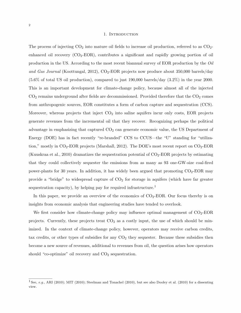
Figure 2. Assumed relationship between CO2 injection, oil production, and CO2 sequestration.

Roil,0 10 Initial recoverable reserves (million barrels)q inj 10 Combined injection of CO2 and water (million barrels/year)pCO2 4 CO2 purchase cost ($/barrel)crec 1 CO2 recycling cost ($/barrel)coth 1 Other costs ($ million)I 27 Up-front capital cost of switching to CO2 flood ($ million)r 5 Discount rate (%/year)

Table 1. Baseline parameter values.

the reservoir that the slugs of CO2 sweep through, by reducing the tendency of CO2 to “finger” or

“channel” between injection and production wells, bypassing some of the oil.4

The second assumption reflects the fact that both injected fluids end up occupying the pore

space vacated by produced oil. It seems reasonable that they should end up doing so roughly in

proportion to their ratio in the injection mix.

Figure 2 shows the relationship between the CO2 injection rate and the oil production and

CO2 sequestration rates implied by these assumptions, if the δ function is a simple quadratic

δ(f injCO2,t) = 0.06 + 0.2f injCO2,t

− 0.16(f injCO2,t)2.

Importantly, this functional form and its coefficients are merely illustrative: although they are

loosely based on data from a simulation study by Guo et al. (2006) as well as on experience at the

Lost Soldier-Tensleep EOR project in Wyoming, the actual shape of the functions is likely to be

highly dependent on the specific properties of any given reservoir and of the oil it contains.

4 See, e.g., Al-Shuraiqi et al. (2003), Jessen et al. (2005b), Juanes and Blunt (2006), Guo et al. (2006), and Trivediand Babadagli (2007).

8

0 10 20 30 40 50

0

1

2

3

4

5

6

Time (years)

Flo

ws (

mill

ion b

l/year)

CO2 injection

oil production

CO2 sequestration

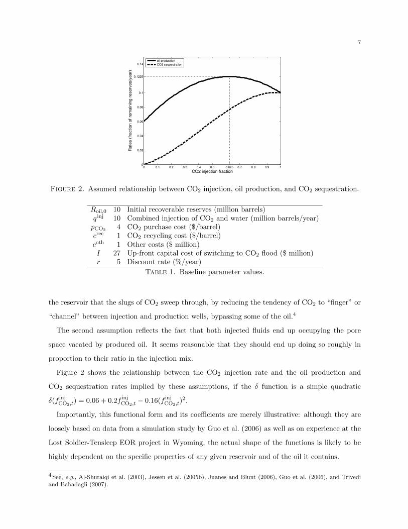
Figure 3. Baseline simulation results.

The full model consists of objective function (5), equations (6) and (7), and an equation Roil,t+1 =

Roil,t − qprdoil,t to update remaining reserves in each period. Using the parameter values given in

Table 1,5 we solve the model numerically for the combination of terminal time T and vector of CO2

injection rates qinjCO2,0, qinjCO2,1

, qinjCO2,2, · · · , qinjCO2,T

up to that time that maximize NPV.

Figure 3 shows the result at our baseline oil price of $100/bl and baseline CO2 sequestration

subsidy of $4/bl (≈ 40/tCO2). At these values, it is optimal to intially inject a mix of about 50%

CO2 and water, but to gradually drop the CO2 fraction over time. After 22 years, the optimal

fraction drops to zero, after which the project optimally continues to operate for another 31 years

(so the optimal terminal time T is 53 years) while injecting only water.

Paradoxically, when we then re-run the simulations for a range of oil prices and CO2 subsidies,

we find that cumulative CO2 sequestration is much more responsive to the oil price than to the

sequestration subsidy. As shown in Figure 4, halving the subsidy to $20/tCO2 reduces cumula-

tive sequestration by only about 5%, while doubling the subsidy to $80/tCO2 increases cumulative

sequestration by only 11%. In contrast, halving the oil price to $50/bl reduces cumulative se-

questration by 36%, and doubling the oil price to $200/bl increases cumulative sequestration by

42%.

5Note that we measure CO2 in barrels rather than the more conventional units of mcf (1,000 cubic feet at standardsurface temperature and pressure conditions) or tCO2 (1 metric tonne). At the temperature and pressure conditionsinside the Lost-Soldier Tensleep reservoir, 1 mcf of CO2 is compressed to about 0.471 barrels, which we round off to0.5 bl/mcf. The standard conversion factor between mcf and tCO2 is about 18.9, which we round off to 20 mcf/tCO2.See Leach et al. (2011) for further details.

9

0 5 10 15 20 25 30 35 40 45

0

0.5

1

1.5

2

2.5

3

3.5

4

4.5

5

Time (years)

Quantity

(m

illio

n b

l)

p $50/bl

p $100/blp $200/bl

(a)

0 5 10 15 20 25 30 35 40 45

0

0.5

1

1.5

2

2.5

3

3.5

4

4.5

5

Time (years)

Quantity

(m

illio

n b

l)

subsidy $20/tCO2

subsidy $40/tCO2subsidy $80/tCO2

(b)

Figure 4. Sensitivity of cumulative sequestration to (a) the oil price (b) the se-questration subsidy.

The reason is quite straightforward: at realistic oil-price and sequestration-subsidy levels, oil

revenues make up a far larger share of a project’s profits than do sequestration revenues. In terms

of equation (4) above, not only is the sequestration rate q injCO2is over most of the project’s lifetime

less than half as large as the oil production rate qprdoil (when both are expressed in comparable units

such as bl/year) but its weight is orders of magnitude smaller: over the range of subsidies and

prices considered in Figure 4, the weight on sequestration varies from $-1 to $5, while that on oil

production varies from $50 to $200. As a result, the operator’s incentive, even with sequestration

subsidies as high as $80/tCO2, is to largely ignore sequestration and instead manage the project

so as to maximize oil production alone.

The relationship between oil production and sequestration shown in Figure 2, however, implies

that increasing oil production even slightly in response to a higher oil price may require injecting,

and hence sequestering, large amounts of additional CO2. For example, we find that if the oil price

doubles from $100 to $200, the operator’s optimal CO2 injection rate over the first 30 years of

the project increases 45%, from 2.26 million bl/year to 3.29 million bl/year. Doing so increases

average oil production by only 2%, from 0.312 million bl/year to 0.318 million bl/year, but this

implies a revenue boost from oil sales of $1.2 million/year. At the same time it increases average

CO2 sequestration by 24%, from 0.126 million bl/year to 0.155 million bl/year, but this implies a

revenue boost from sequestration subsidies of only $0.12 million/year. From the operator’s point

10

of view, then, the boost in CO2 sequestration, while significant in quantity terms, is just a “side

effect” in dollar terms.

Conversely, even very high sequestration subsidies will not induce the operator to alter project

management by much. A true tradeoff between oil revenues and CO2 sequestration emerges only

when the subsidy reaches levels as high as $120/tCO2 (well above realistic levels in the near future),

and even then, the operator will optimally give up only very small amounts of oil production in

order to boost CO2 sequestration. In terms of Figure 2, it is only at these very high CO2 subsidy

levels that the operator will briefly, at the very beginning of the flood, choose a CO2 injection

fraction higher than the oil-production-maximizing fraction of 0.625.

While the preceding result suggests that climate policy should perhaps focus on raising oil prices

rather than on subsidizing CO2 sequestration, we find this need not be the case. There are two

reasons.

First, we find—in an extension of our previous work that incorporates possible changes in oil

prices or CO2 subsidies over time (Leach et al., 2010)—that rapid increases in the oil price, if

anticipated by operators, may greatly reduce sequestration by CO2-EOR projects. As shown in

panel (b) of Figure 5, cumulative sequestration from our model project drops by as much as 53%,

from 3.77 million bl to 1.78 million bl, if instead of staying constant at $100/bl, the oil price

increases at a rate of 7.5% per year.

Underlying this is the fact that large up-front investment costs are required to switch from con-

ventional oil-recovery methods, such as waterflooding, to CO2 injection. That is, the full expression

for the net present value of a project is

NPV = −I +

T∑t=0

1

(1 + r)t

[poil,tq

prdoil,t + (sCO2,t − pCO2,t + crect )qseqCO2,t

− crect q injCO2,t− cotht

], (8)

where I is the up-front investment cost.

In general, oil field operators have an incentive to delay switching in order to delay these invest-

ment costs. When oil prices are anticipated to increase, there is an additional incentive to delay:

by so doing, the CO2-induced boost in oil production is pushed back to a time when oil prices

are higher. But the extension of waterflooding until this later switching time also reduces CO2

sequestration. This is because reservoir pore space that would have been occupied by CO2 had

EOR commenced sooner will now be occupied by water.

11

0 5 10 15 20 25 30 35 40 45

0

1

2

3

4

5

Time (years)

Ra

te (

mill

ion

bl/ye

ar)

p growth 0%

p growth 2.5%

p growth 5%

p growth 7.5%

(a)

0 5 10 15 20 25 30 35 40 45

0

1

2

3

4

5

Time (years)

Qu

an

tity

(m

illio

n b

l)

p growth 0%

p growth 2.5%

p growth 5%

p growth 7.5%

(b)

Figure 5. Sensitivity of cumulative sequestration to (a) the oil price (b) the se-questration subsidy.

Second, and independent of the first effect, when the incremental oil recovered by EOR projects

is consumed, additional CO2 emissions will be generated. A common misconception is that these

emissions can be ignored, ostensibly because incremental oil from EOR merely “displaces” conven-

tionally produced oil.

In their study of net sequestration by eight North American CO2-EOR projects, Faltinson and

Gunter (2011) suggest, for example, that

“Project-life-cycle emissions attributed to CO2 EOR should include fugitive emis-sions directly related to the CO2-EOR project only, and not include downstreamemissions common to all sources of oil supply.”

This is because, they argue,

“World oil production is determined by world oil demand and if CO2-EOR projectswere not undertaken, some other source of oil would step forward and fill the gap.Therefore, executing CO2-EOR projects will not result in incremental aggregaterefining and consumption emissions” (emphasis added).

This line of reasoning presumes, however, that aggregate world demand for oil is fixed, i.e.,

perfectly insensitive to price. If so, any drop in the oil price caused by increasing EOR supply will

induce no expansion of demand, forcing marginal conventional oil projects to cut back production

by exactly the amount of EOR production added. Realistically, however, world demand is price

12

sensitive (particularly in the long run), and incremental EOR production therefore does expand

aggregate consumption and emissions.

3. Market Equilibria

We provide a graphical illustration of the oil market, based on the model previously described. For

expositional simplicity, we discuss only the first two periods of a multi-period story. In this setting,

we refer to the current time frame as “period 0” and the future as “period 1.” At the start of a

given period t, firms collectively have remaining reserves rcont , where the superscript indicates that

these reserves have been developed using conventional technology. Of these reserves, at most a

given proportion δ can be extracted. Under a wide range of conditions, this constraint will bind,

allowing us to focus on the role played by current “developed” reserves. To produce a greater level

of output, new reserves must be added to the portfolio, a process that involves exploration and

development. Here we do not describe these steps in any detail; rather, we focus on the impact

these “additions” acon will have on the problem.

Adding reserves is costly, with the total cost given by c(acon, Acon), where Acon is cumulative

additions at the current time. One can think of a story in which the relatively easy to find and

develop reserves are added sooner, in which case the costs of adding reserves naturally rise as

cumulative additions mount. With this intuition in mind, we assume cA > 0; it is also natural to

assume that adding more reserves is costly, given any particular level of accumulated additions, so

that ca > 0 as well.

In deciding what level of additions to bring forward at time 0, the (discounted) stream of oper-

ating profits is compared against the (up front) development costs; this implies a cutoff price, p0,

that would just generate the requisite stream of profits. Viewed through this lens, one can think

of the incremental cost of bringing forward greater levels of additions as comprising an increasing

supply schedule. We denote the available reserves in period t (after the new additions are brought

on line) as Rcont ≡ rcont + acont ; based on these available reserves, output is Qcon

t = δRcont . Within

the period, the market equilibrium price equates the incremental cost associated with this supply

schedule to the willingness to pay for that last barrel of oil, as reflected by the market demand

curve.

13

Scon0

p0

Qcon0

D

p

Qoil

poil

x

x

(a)

Scon0

p0

Qcon0

Scon1

p1

Qcon1

D

p

Qoil

poil

x

x

(b)

Scon0

Scon+EOR0

p′0

Q′0con+EOR

p0

Qcon0Q′

0con

displacedconventionalproduction D

p

Qoil

poil

x

x

(c)

Scon0

Scon+EOR0

p′0

Q′0con+EORQ′

0con

displacedconventionalproduction

Scon1

Scon+EOR1

p′1 = p0

Q′1con+EOR

(= Qcon0 )

Q′1con

previouslydisplaced

conventionalproduction D

p

Qoil

poil

x

x

(d)

Figure 6. Stylized representation the world oil market at two periods in time,without (panels (a) and (b)) or with additional production from CO2-EOR (panels(c) and (d)).

Writing the optimal level of new additions in period 0 be acon0 , total output delivered to market

is then Q0 = δ(rcon0 + acon0 ). The market-equilibrium price corresponding to this level of output,

illustrated in panel (a) of Figure 6, is p0.

Now consider the next period. The remaining reserves at the start of the period are rcon1 =

(1 − δ)Rcon0 , the fraction of period-0 available reserves that was not extracted. Again, firms may

add to these reserves, up to the point where the last barrel added brings a profit stream that

just covers the current development cost. Because the depletion effect associated with period

0 production reduces the amount that can be produced in period 1, the supply curve shifts in

14

(leftward) between periods 0 and 1.6 As a result, the market equilibrium price increases from p0 to

p1. This point is illustrated in panel (b) of Figure 6.

In this framework, imagine firms discover the potential to add to reserves via CO2-EOR. This

technique is similar to additions, in that it raises the available stock of reserves, but it is cheaper

to incorporate. The increased production that EOR facilitates induces an outward tilting of the

supply curve, above some new threshold price; panel (c) of Figure 6 illustrates. With this new

supply curve, the market equilibrium price falls and equilibrium quantity rises.7

Importantly, the increase in market quantity implies that the new output associated with EOR

must more than offset the reduction in output from conventional sources that are not brought to

market in period 0. That is, the oil production “displaced” by EOR is smaller than the increase due

to EOR, contrary to arguments that have been made. Note too that this “displaced” production is

associated with new additions that are no longer economic as a result of the lower price that follows

naturally from the increase in supply arising from EOR. While these additions are not brought on

line in period 0, they are nevertheless still available in the future.

Because of the upward-sloping nature of the incremental cost curve for additions, some additions

to conventional developed reserves remain economic even with the lower price; call the correspond-

ing optimal level of additions a′con0 . The net effect on output in period 0 is an increase, from

Qcon0 = δRcon

0 = δ(rcon0 + acon0 )

to

Q′con+EOR0 = δR′con+EOR

0 = δ(rcon0 + a′con0 + aEOR0 ).

At the start of period 1, remaining reserves are now

r′con+EOR1 = (1 − δ)R′con+EOR

0 = (1 − δ)(rcon0 + a′con0 + aEOR0 ),

and so if without any further additions, supply would equal

δr′con+EOR1 = δ(1 − δ)(rcon0 + a′con0 + aEOR

0 ).

6 In addition, the time horizon is shorter (the backstop is more imminent) in period 1, so there is a shorter time frameto enjoy these profits, which raises the price required to motivate development must be greater than it was in period0. This effect is of second-order importance in our scenario, and so we abstract from it in the pursuant discussion.7This reduction in price obtains so long as demand is not perfectly elastic.

15

This supply level corresponds to the intercept of the supply curve labeled Scon+EOR1 in panel (d) of

Figure 6. The supply curve labeled Scon1 represents the component of overall supply that is provided

by conventional sources, and has intercept

δr′con1 = δ(1 − δ)(rcon0 + a′con0 ).

Because at p′0, demand exceeds δr′con+EOR1 , the new market equilibrium entails a higher price

p′1. To avoid clutter, we have set this price to correspond with the original period-0 price in the

absence of EOR, p0.8

At this price p′1 = p0, further additions to both conventional and EOR reserves become economic

and are brought into production. Importantly, by our convenient assumption that p′1 = p0, the

period-1 additions to conventional reserves that become economic, a′con1 , are precisely those addi-

tions that would have been economic in period 0 in the absence of EOR, but became uneconomic as

a result of the price drop from p0 to p′0. That is, a′con1 = acon0 −a′con0 . It follows that the conventional

production out of these additions that would have been supplied in period 0, but was displaced,

becomes part of overall production in period 1. The displacement is therefore only temporary: in

this case it merely involves a one-period delay.

More generally, the ultimate impact of CO2-EOR upon cumulative oil production depends on

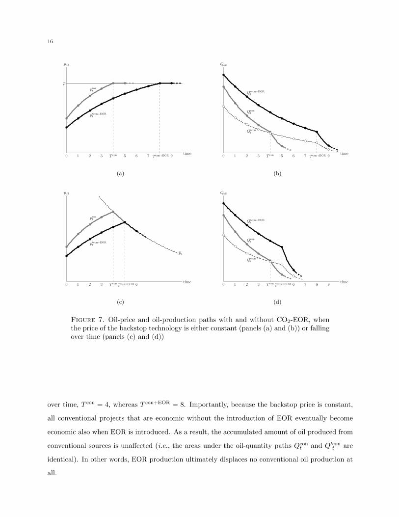
the impacts in multiple periods. Panel (a) of Figure 7 compares the oil-price path with only

conventional production, pcont , to that with added production from CO2-EOR, p′con+EORt . Let T con

and T con+EOR denote the times at which the oil price reaches p in the scenario without and with

CO2-EOR, respectively. Under both scenarios, the oil price increases over time. However, the

addition of CO2-EOR production raises production in each period, as illustrated in panel (b) of

Figure 7. In every such period, the increased production implies a lower price, and so the oil-price

path p′con+EORt lies below the oil-price path pcont in panel (a).

At a certain point, each path hits a price ceiling p, above which oil demand drops to zero. This

is because p represents the price of a renewable, “backstop” technology that is a perfect substitute

for oil. At this price, oil production may still continue for some time, but no additions to reserves

are made. Since the path p′con+EORt lies below the path pcont , it follows that T con+EOR > T con. In

the example illustrated in panels (a) and (b) of Figure 7, where the backstop price does not change

8Of course, this scenario is coincidental. But our central point, that the net effect of introducing EOR will only beneutral in terms of the impact on ultimate oil production under very special circumstances, does not depend on thisgraphical assumption.

16

0 1 2 3 T con 5 6 7 T con+EOR 9

p

pcont

p′tcon+EOR

time

poil

x

x

(a)

0 1 2 3 T con 5 6 7 T con+EOR 9

Qcont

Q′tcon+EOR

Q′tcon

time

Qoil

x

x

(b)

0 1 2 3 T con T con+EOR 6

pt

pcont

p′tcon+EOR

time

poil

x

x

(c)

0 1 2 3 T con T con+EOR 6 7 8 9

Qcont

Q′tcon+EOR

Q′tcon

time

Qoil

x

x

(d)

Figure 7. Oil-price and oil-production paths with and without CO2-EOR, whenthe price of the backstop technology is either constant (panels (a) and (b)) or fallingover time (panels (c) and (d))

over time, T con = 4, whereas T con+EOR = 8. Importantly, because the backstop price is constant,

all conventional projects that are economic without the introduction of EOR eventually become

economic also when EOR is introduced. As a result, the accumulated amount of oil produced from

conventional sources is unaffected (i.e., the areas under the oil-quantity paths Qcont and Q′cont are

identical). In other words, EOR production ultimately displaces no conventional oil production at

all.

17

If, on the other hand, the backstop price falls over time, matters are more complex.9 In this

scenario, the outward shift in the oil price implies that there is more time for the backstop price to

decline, and as a result the backstop is reached at a lower price. Panel (c) of Figure 7 illustrates this

point. This lower “terminal” oil price in turn induces a reduction in cumulative additions (i.e., the

area under the oil-quantity path Q′cont in panel (d) is smaller than the area under the oil-quantity

path Qcont ). Ultimately, the net effect on total production turns on a comparison of this induced

reduction on the one hand with the increased output associated with EOR on the other.

4. conclusion

In this paper, we have investigated the impact of EOR on oil markets, paying specific attention

to the interplay of supply and demand across time. A key result is that the introduction of EOR

displaces oil production early on, as the lower prices that result from a supply expansion render some

potential additions uneconomic. But over time, as depletion occurs and prices rise, the erstwhile

displaced projects become economic. Accordingly, the introduction of EOR may not displace any

production, though it necessarily will delay the development of some new sources of production. In

the end, then, introduction of EOR will necessarily increase the total accumulated amount of oil

produced. As any extra oil produced will ultimately yield CO2 emissions, a key issue is how the

extra CO2 emissions associated with the net increase in oil extraction compares to the amount of

CO2sequestered by EOR.

If the critical price at which the economy switches from oil to another energy source, which we

have referred to as the backstop price, is constant across time, then it follows that all production

that would have obtained if EOR were never introduced will also (eventually) be brought on line

after EOR is introduced. The end result is that the introduction of EOR must necessarily raise

total accumulated oil production by the time the backstop is adopted, with the amount of extra

production corresponding to the level of oil produced by EOR. If the level of CO2 sequestered by

EOR is roughly equivalent to the amount of CO2 generated by the consumption of this extra oil

produced, then introducing EOR has no net effect on carbon emissions. By contrast, if the backstop

price falls over time, as one might expect if learning occurs over time, and if this learning makes

9 There is, we believe, good reason to expect the backstop price to fall: historically, R&D into technologies associatedwith renewable resources have produced striking cost reductions over time. If this pattern is indicative of likely trendsgoing forward, then there seems to be good reason to anticipate the backstop price will decline over time.

18

the new technology more efficient, then some of the projects that are pushed out of the market

after the introduction of EOR will never be developed. The implication is that the increase in total

accumulated amount of oil produced is smaller than that described in the previous paragraph. It

then follows that introducing EOR leads to a net reduction in the accumulated amount of CO2

emitted over time.

In linking the impact of EOR upon carbon stocks, it is tempting to think that the timing of

production changes is of paramount importance. But such an approach presumes that damages are

linked to carbon stocks (indeed, the typical Integrated Assessment Model follows this approach).

But if damages are linked to temperatures, as seems most likely, then the key question is: what

effect does a change in the stream of emissions have upon the time path of temperatures? In this

regard, Allen et al. (2009) have argued that it is the cumulative amount of CO2 emitted by, say,

2050 that is of crucial importance, with the time path of those emissions being far less critical.

Taking this perspective, the key consideration in evaluating the impact of EOR upon damages is

the net effect on cumulative emissions over time.

This then raises the policy question of how to address the fact that, due to both geological factors

and differing management practices, net CO2 emissions by EOR projects vary widely. Whereas some

projects sequester far less CO2 per incremental barrel than the consumption of those barrels will

generate, other projects sequester more (therefore arguably producing “green” oil). Presumably,

one would want a policy to discourage the former class of projects, while promoting the latter class

of projects. Fortunately, a comprehensive tax on CO2 emissions (or an equivalent cap-and-trade

scheme) will accomplish both objectives. It does so indirectly, through induced adjustments in the

oil and CO2 markets that reduce both the oil price that EOR projects receive and the CO2 price

that they pay. A large enough tax will in fact make that CO2 price negative, thereby effectively

acting as a sequestration subsidy. Moreover, these price adjustments will appropriately account

for market switching between energy sources, thereby making the above-described “displacement”

issue moot.

References

Al-Shuraiqi, H. S., Muggeridge, A. H. and Grattoni, C. A. (2003). Laboratory investigations of first contact

miscible WAG displacement: The effects of WAg ratio and flow rate, Working Paper 84894, Society of

Petroleum Engineers (SPE).

19

Allen, M. R., Frame, D. J., Huntingford, C., Jones, C. D., Lowe, J. A., Menihausen, M. and Meinhausen, N.

(2009). Warming caused by cumulative carbon emissions towards the trillionth tonne, Nature 458: 1163–

1166.

ARI (2010). U.S. oil production potential from accelerated deployment of carbon capture and storage.

Advanced Resources International, White Paper prepared for Natural Resources Defense Council.

Asghari, K. and Al-Dliwe, A. (2004). Optimization of carbon dioxide sequestration and improved oil recovery

in oil reservoirs, GHGT-7 Proceedings.

Babadagli, T. (2006). Optimization of CO2 injection for sequestrationenhanced oil recovery and current

status in canada, Advances in the Geological Storage of Carbon Dioxide, Springer, pp. 261–270.

Dooley, J., Dahowski, R. and Davidson, C. (2010). CO2-driven enhanced oil recovery as a stepping stone to

what?, Technical Report PNNL-19557, Pacific Northwest National Laboratory.

Faltinson, J. and Gunter, B. (2011). Net CO2 stored in North American EOR projects, Journal of Canadian

Petroleum Technology 50(7/8): 55–60.

Forooghi, A., Hamouda, A. and Eilertsen, T. (2009). Co-optimization of CO2 EOR and sequestration in a

North Sea chalk reservoir. SPE 125550.

Ghomian, Y., Sepehrnoori, K. and Pope, G. (2010). Efficient investigation of uncertainties in flood design

parameters for coupled CO2 sequestration and enhanced oil recovery. SPE 1397380.

Guo, X., Du, Z., Sun, L. and Fu, Y. (2006). Optimization of tertiary water-alternate-CO2 flood in Jilin oil

field of China: Laboratory and simulation studies, Working Paper 99616, Society of Petroleum Engineers

(SPE).

Jahangiri, H. R. and Zhang, D. (2011). Optimization of the net present value of carbon dioxide sequestration

and enhanced oil recovery. OTC 21985.

Jessen, K., Kovscek, A. R. and Orr Jr., F. M. (2005a). Increasing CO2 storage in oil recovery, Energy

Conversion and Management 46: 293–311.

Jessen, K., Kovscek, A. R. and Orr Jr., F. M. (2005b). Increasing CO2 storage in oil recovery, Energy

Conversion and Management 46: 293–311.

Juanes, R. and Blunt, M. J. (2006). Analytical solutions to multiphase first-contact miscible models with

viscous fingering, Transport in Porous Media 64: 339–373.

Koottungal, L. (2012). 2012 worldwide EOR survey, Oil & Gas Journal 110(4): 57–69.

Kovscek, A. and Cakici, M. (2005). Geologic storage of carbon dioxide and enhanced oil recovery. ii. coop-

timization of storage and recovery, Energy Conversion and Management 46: 1941–1956.

Kuuskraa, V., Van Leeuwen, T. and Wallace, M. (2010). Improving domestic energy security and lower-

ing CO2 emissions with ‘next generation’ CO2-enhanced oil recovery (CO2-EOR). US Department of

Energy/National Energy Technology Laboratory, DOE/NETL-2011/1504.

Leach, A., Mason, C. F. and van ’t Veld, K. (2010). Co-optimization of enhanced oil recovery and carbon

sequestration, Climates of Change: Sustainability Challenges for Enterprise Working Paper 005, Smith

20

School of Enterprise and the Environment, University of Oxford, UK.

Leach, A., Mason, C. F. and van ’t Veld, K. (2011). Co-optimization of enhanced oil recovery and carbon

sequestration, Resource and Energy Economics 33: 893–912.

Marshall, C. (2012). DOE unveils new strategy, mapping system to advance carbon storage. ClimateWire,

http://www.eenews.net/climatewire/2012/05/02/archive/3.

MIT (2010). Role of enhanced oil recovery in accelerating the deployment of carbon capture and sequestra-

tion, Symposium report, Mit Energy Initiative and Bureau of Economic Geology at UT Austin.

Pamukcu, Y. and Gumrah, F. (2009). A numerical simulation study of carbon-dioxide sequestration into a

depleted oil reservoir, Energy Sources, Part A 31: 1348–1367.

Steelman, J. and Tonachel, L. (2010). Reducing imported oil with comprehensive climate and energy legis-

lation. Natural Resources Defense Council, Washington, DC.

Trivedi, J. J. and Babadagli, T. (2007). Optimal injection strategies for CO2 and flue gas sequestration

during tertiary oil recovery, Oil Gas–European Magazine 33(1): 22–26.