The Economic Returns to Social Interaction:

Experimental Evidence from Microfinance

Benjamin Feigenberg, Erica Field and Rohini Pande⇤

February 23, 2013

Abstract

Microfinance clients were randomly assigned to repayment groups that met eitherweekly or monthly during their first loan cycle, and then graduated to identicalmeeting frequency for their second loan. Long-run survey data and a follow-uppublic goods experiment reveal that clients initially assigned to weekly groups in-teract more often and exhibit a higher willingness to pool risk with group membersfrom their first loan cycle nearly two years after the experiment. They were alsothree times less likely to default on their second loan. Evidence from an additionaltreatment arm shows that, holding meeting frequency fixed, the pattern is insen-sitive to repayment frequency during the first loan cycle. Taken together, thesefindings constitute the first experimental evidence on the economic returns to so-cial interaction, and provide an alternative explanation for the success of the grouplending model in reducing default risk.

JEL: C81,C93, O12, O16

⇤The authors are from MIT (Feigenberg), Duke University (Field) and Harvard University (Pande).We thank Max Bode, Emmerich Davies, Sean Lewis Faupel, Sitaram Mukherjee and Anup Roy forsuperb field work and research assistance, Alexandra Cirone and Gabe Sche✏er for editorial assistanceand Village Financial Society and Centre for Micro Finance for hosting this study, Theresa Chen, AnnieDuflo, Nachiket Mor and Justin Oliver for enabling this work and ICICI, Exxon Mobil Educating Womenand Girls Initiative (administered through WAPP/CID at Harvard) and the Dubai Initiative for financialsupport. We thank the editor, two anonymous referees and Attila Ambrus, Abhijit Banerjee, Tim Besley,Amitabh Chandra, Esther Duflo, Raquel Fernandez, Seema Jayachandran, Dean Karlan, Asim Khwaja,Dominic Leggett, Muriel Niederle, Aloysius Sioux, Jesse Shapiro and numerous seminar participants forhelpful comments.

1

1 Introduction

Social capital, famously defined by Putnam (1993) as “features of social organization,

such as trust, norms and networks, that can improve the e�ciency of society by facili-

tating coordinated actions,” is considered particularly valuable in low-income countries

where formal insurance is largely unavailable and institutions for contract enforcement

are weak.1 Since economic theory suggests that repeat interaction among individuals can

help build and maintain social capital, encouraging interaction may be an e↵ective tool

for development policy. Indeed, numerous development assistance programs emphasize

social contact among community members under the assumption of significant economic

returns to regular interaction. But can simply inducing individuals to interact with one

another actually facilitate economic cooperation?

Rigorous evidence on this question remains limited, largely due to the di�culty of

accounting for endogenous social ties (Manski, 1993, 2000). For instance, if more trust-

worthy individuals or societies are characterized by denser social networks, we cannot

assign a causal interpretation to the positive association between community-level social

ties and public good provision. For similar reasons, it is also not possible to assign a

causal interpretation to the higher levels of cooperation observed among friends relative

to strangers in laboratory public goods games.2 In short, without randomly varying so-

cial distance, it is di�cult to validate the model of returns to repeat interaction and

even harder to determine whether small changes in social contact can produce tangible

economic returns.

The first contribution of this paper is to undertake exactly this exercise. By randomly

varying how often individuals meet, we provide causal evidence on the returns to repeat

social interaction. We do so in the context of a development program that emphasizes

1For instance, Guiso et al. (2004) demonstrate that residents in high social capital regions undertakemore sophisticated financial transactions, and Knack and Keefer (1997) show that a country’s level oftrust correlates positively with its growth rate.

2The community ties literature includes Costa and Kahn (2003); Alesina and La Ferrara (2002);DiPasquale and Glaeser (1999); Miguel et al. (2005); Olken (2009), while laboratory games literatureincludes Glaeser et al. (2000); Carter and Castillo (2004b); Do et al. (2009); Karlan (2005); Ligon andSchechter (2011).

2

group interaction: microfinance.3 In the typical “Grameen Bank”-style microfinance pro-

gram, clients meet weekly in groups to make loan payments. Our experiment varied social

interaction by randomly assigning 100 first-time borrower groups of a typical microfinance

institution (MFI) in India to either meet on a weekly or a monthly basis throughout their

ten-month loan cycle. Using administrative and survey data we study the e↵ect of short-

run increases in group meeting frequency on long-run social contact and an important

measure of economic vulnerability: default incidence in the subsequent loan cycle.

A second contribution of this paper is to identify a key mechanism through which

group lending sustains high repayment rates: risk-pooling among clients. While the

theoretical literature largely emphasizes the importance of joint-liability contracts for

reducing default in microfinance, recent experimental evidence suggests that joint liability

per se has little impact on default (Gine and Karlan, 2011), raising anew the question

of how exactly group lending achieves risk reduction without collateral. Since our clients

received individual-liability debt contracts, we can isolate how a less noted feature of

the classic group lending contract – encouraging social interaction via group meetings –

reduces default.4 In other words, even absent the explicit incentives for monitoring and

enforcement that joint liability provides, frequent group meetings can lower lending risk by

increasing social interaction among group members and, as a consequence, strengthening

3Related work include Dal Bo (2005) who provide laboratory game evidence on returns to repeat eco-

nomic interaction, where the likelihood of future rounds of exchange is randomly assigned and Humphreyset al. (2009)’s field experiment which shows that community development programs randomly assignedto villages encourage pro-social behavior (but cannot isolate the influence of social interaction from otherprogram aspects).

4The remarkable success of microfinance in achieving very high repayment rates on collateral-freeloans to poor individuals is widely recognized, as evidenced by awarding of the Nobel Peace Prize tothe Grameen Bank founder. Our findings complement theoretical research on the role of social collateralin microfinance and empirical work that identifies a significant correlation between social connectionsand default risk (Besley and Coate, 1995; Ghatak and Guinnane, 1999; Karlan, 2005). For instance, MFIclients in Peru who are more trustworthy in a trust game are less likely to default, and group-level defaultis lower in groups where clients have stronger social connections (Karlan, 2005, 2007). In Gine and Karlan(2011), the shift from joint to individual liability increased default among borrowers with ex-ante weaksocial ties. Fischer and Ghatak (2010) show that microfinance repayment schedules are attractive topresent-biased borrowers and consistent with this, Bauer et al. (2012) shows that microfinance borrowersare relatively more likely to be present-biased. It is likely that microfinance induced gains in socialcollateral, which improve informal insurance arrangements, are particularly valued by these borrowers.In our setting, Field et al. (forthcoming) show that impatient borrowers benefit less from added flexibilityin the form of a grace period.

3

risk-pooling arrangements within social networks.

Our evidence consists of several striking changes in client behavior associated with

experimentally increasing the frequency of client contact. First, clients assigned to weekly

groups during their first loan cycle increased social contact with group members outside

of meetings, and sustained it in the long run. More than a year after the experiment

ended, clients who had met on a weekly basis during their first loan saw each other

37% more often outside of group meetings. If client groups remained fixed for multiple

loan cycles, then treatment and control groups should converge in terms of their degree

of connectedness, in which case we would no longer observe long-run di↵erences in the

degree of social interaction according to first-intervention meeting frequency. Instead, the

persistence of the di↵erence makes sense in our setting given that, due to a policy change

immediately after our experiment that reduced loan groups from ten to five members,

the majority of pairs (68%) of first loan group members were no longer in the same loan

group at follow-up. As our long-run social contact data show, clients continue to interact

outside of loan groups and treatment clients do so at a significantly higher rate.

Second, greater social interaction among clients on a weekly schedule was accompanied

by increased willingness to pool risk relative to monthly clients. Here, our evidence comes

from a field-based lottery game conducted roughly 16 months after the first loan cycle

ended. The lottery operated much like a laboratory trust or solidarity game, but in a

real-world setting. Each client was entered into a (separate) promotional lottery for the

MFI’s new retail store. The client started with a 1 in 11 chance of winning the lottery

prize, a voucher redeemable at the MFI store. She was then o↵ered the opportunity to

give out additional lottery tickets to any number of members of her first loan group.

Since ticket-giving reduces a client’s individual chances but increases the probability

that someone from the group would win, it captures either her unconditional altruism

towards or willingness to risk-share with members of her initial group. To distinguish

insurance motivations from unconditional altruism, we randomized the divisibility of the

lottery prize. Assuming the more easily divisible prize reduces transaction costs of sharing

and/or is perceived as more conducive to sharing, then a client should give more tickets

4

when the prize is divisible if she is motivated at least in part by risk-sharing considerations,

but should not if her sole motivation is unconditional altruism.5

Relative to a monthly client, a client who had been assigned to a weekly group two

years prior was 32% more likely to enter a group member into the lottery when the prize

was divisible, but only 16% more likely when it was not.

Finally, we show that clients on a weekly schedule were, in the long run, better able

to endure financial shocks. Those who met weekly during their first loan cycle were three

times (5.2 percentage points) less likely to default on their subsequent loan, despite the

fact that all clients had reverted to the same repayment schedule.

To disentangle the role of meeting frequency from repayment frequency, we use a

second treatment arm in which clients were assigned to meet weekly but maintained a

monthly repayment schedule. To address variation in actual occurrence of non-repayment

meetings in this arm, we implement an Instrumental Variable (IV) strategy, which exploits

the fact that loan o�cers were more likely to cancel a non-repayment meeting on days

with heavy rainfall. Our IV estimates show that the default rate di↵erence remains in

magnitude and significance when we compare monthly clients to clients randomly assigned

to meet weekly but repay monthly. Based on this evidence, we conclude that default risk

falls on account of meeting more frequently rather than di↵erences in fiscal habits that

could arise from requiring clients to initially repay at more frequent intervals.

To summarize, a higher degree of short-run interaction is associated with increased

social interaction in the long run, improved risk-sharing arrangements among clients and

lower default. Our findings are consistent with several mechanisms through which social

interactions reduces default, including improved monitoring, better information flows,

lower transaction costs for risk-sharing and better ability to punish potential deviations

from risk-sharing, which we are unable to disentangle. However, our findings substanti-

ate theoretical claims that repeat interaction can yield economic returns by facilitating

5Similar variations of dictator or trust games have been used to parse out motives for giving (Ligonand Schechter, 2011; Do et al., 2009; Carter and Castillo, 2004a). Most similar to us, Gneezy et al. (2000)use a sequence of trust games with varying constraints on the amount that can be returned to show thatindividuals contribute more when large repayments are feasible.

5

informal economic exchange, and provide an alternative explanation for the success of

the group lending model. More generally, the findings demonstrate that tweaking the

design of standard development programs to encourage social interaction can generate

economically valuable social capital.

The paper is structured as follows: Section 2 describes the experimental design. Sec-

tion 3 examines how randomized di↵erences in meeting frequency, implemented only dur-

ing the first loan cycle, influenced long-run social interaction and client willingness to share

in the field lottery. Section 4 documents changes in long-run default rates and separates

the role of meeting frequency from that of repayment frequency. Section 5 concludes.

2 Experimental Design

2.1 Setting

Our MFI partner, Village Financial Services (VFS), operates in the Indian state of West

Bengal. In 2006 when we began our field experiment, it had $6.75 million in outstanding

loans to over 56,000 female clients. VFS’ gross loan portfolio to total asset ratio of 78%

placed it slightly below the median Indian MFI (84%) while its portfolio at risk of 0.47%

(defined as payments outstanding in excess of 30 days) was identical to the median Indian

MFI (MIX Market, 2012).

Our study population consisted of first-time VFS clients living in peri-urban slums of

the city of Kolkata. At the time of joining the MFI, over 70% of client households owned a

business and the median client’s household income placed her just below the dollar-a-day

poverty line. Study population demographics, such as income, home ownership and home

size, are largely comparable with similar MFIs operating in other Indian cities (Online

Appendix Table 2). However, consistent with cross-city di↵erences in MFI penetration,

clients in our sample exhibit significantly lower rates of borrowing outside of the MFI.

6

2.2 Sample

Between April and September 2006 we recruited 100 first-time microfinance groups from

neighborhoods in the catchment areas of three VFS branches. Following VFS protocol,

the loan o�cer first surveyed the neighborhood and then conducted a meeting to inform

female residents about the VFS loan product. Interested women were invited for a five-

day training program, where clients met for an hour each day and learned about the

benefits and responsibilities of the loan. At the end of the five days, the loan o�cer

assigned women into groups of ten and identified a leader of each group.6 Thus, clients in

a single loan group lived in close proximity and were typically acquainted prior to joining.

Although 63% of group members in our sample knew one another at group formation,

most described their relationship with other group members as neighbors (48%) rather

than friends (7%) or family (8%).

2.3 Experimental Design

Group Assignment At the end of the group formation process, each group member

was o↵ered an individual-liability loan of Rs. 4,000 (⇠$100) and told that her repayment

schedule would be assigned at the time of loan disbursal. Prior to loan disbursal, groups

were randomized into either weekly or monthly schedules. In total, 38 groups were as-

signed to the control arm in which group meetings were held on a monthly basis, and

30 groups were assigned to the treatment arm in which group meetings occurred weekly

(Treatment 1). In addition, 32 groups were assigned to an alternative treatment in which

they met weekly but repaid monthly (Treatment 2), an artificial contract design for the

purpose of microfinance delivery, but one that allows us to disentangle the influence of

meeting frequency from the influence of repayment frequency for scientific purposes.

At loan disbursal, Treatment 1 groups were informed that they were to repay their

loans in 44 weekly installments of Rs. 100 (a reasonably small amount given average

weekly household earnings of Rs. 1,167), while Control and Treatment 2 groups were told

6Loan o�cers aimed to form ten-member groups. In practice, group size ranged between nine andthirteen members, with 77% ten-member groups.

7

that they would repay in 11 monthly installments of Rs. 400. No client dropped out after

her repayment schedule was announced.

Meeting Protocol Repayment in a group setting is an integral part of MFI lending prac-

tice, and VFS followed a relatively standard “Grameen Bank” group meeting model. Each

group was assigned a loan o�cer who conducted the meeting in the group leader’s house.

The average meeting lasted 18 minutes, during which clients took an oath promising reg-

ular repayment, and deposited payment with the loan o�cer and had their passbooks

marked.7 Thus, a client’s repayment behavior was observable to other group members,

although in practice most clients socialized while awaiting their turn. Anecdotally, social-

izing happens en route to meetings, while waiting for the loan o�cer to arrive and begin

meetings and while waiting for one’s turn to pay.8

Overall, Control and Treatment 1 groups closely followed the assigned meeting sched-

ule: No Control group met less than five or more than eleven times and no Treatment 1

group met less than 23 or more than 44 times, which were the minimum and maximum

meetings allowed by the respective contracts.9 While in theory clients could skip meetings

and send their payment with another group member, it was rare for clients to do so, and

average attendance at repayment meetings was 81%.

Treatment 2 groups did not strictly adhere to the experimental protocol: Only half

of the groups met at least the minimum required number of times (23) and average

attendance at meetings was only 56%. As this compliance issue necessitates a more

complicated econometric strategy, we first present experimental estimates which compare

Control and Treatment 1 groups only. Then, in order to identify the channels of influence,

in Section 4.1.2 we reintroduce Treatment 2 and describe our econometric approach to

isolate compliers in this arm.

7While the oath encourages group responsibility for loans, the loan contract is individual liability.8Anthropologists have also documented that group lending increases women’s opportunities for social

interaction with members of their community (Larance, 2001).9Variation in number of meetings within a repayment schedule reflects the fact that VFS allows a

client to repay her outstanding balance in a single installment starting 23 weeks after loan disbursement.Once a majority of group members have repaid, remaining clients typically repay at the VFS o�ce.

8

2.4 Data

We tracked our experimental clients over two and a half loan cycles (on average 176

weeks). Figure 1 provides a detailed study timeline. Our analysis makes use of several

data sources, which we describe in turn.

Baseline and Endline Data After group formation, we administered a baseline sur-

vey to 1016 out of 1028 clients. The short time period between group formation and

loan disbursement led to a significant fraction of baseline surveys taking place after loan

disbursement. We therefore exclude any potentially endogenous baseline variables from

the analysis. Roughly 13 months after first loan disbursement, we conducted an endline

survey with 961 clients that provides data on transfers and loan use. We observe similar

attrition in both surveys across treatment and control clients (Online Appendix Table 3).

Short-run Social Contact To gauge social interaction among group members, loan o�-

cers collected data at repayment meetings during the first loan cycle. The protocol was as

follows: After marking passbooks, each client was pulled aside and asked broad questions

about social ties with other group members, in order to provide multiple indicators of

short-run contact. The first two of these indicators measure social interaction and are

constructed as the maximum values of client responses to the two questions – “Have all of

your group members visited your house?” and “Have you visited the houses of all group

members?” The next two indicators measure knowledge of group members: whether the

client knew the names of her group members’ immediate family and whether she knew if

group members had relatives visit over the previous month.10 Here, we report the average

e↵ect size across these measures, defined as the short-run social contact index.11

10To preserve anonymity (given potential observability of responses by group members) we did not askabout interactions with specific group members. We consider the maximum value for all variables, exceptthe relative visit variable for which we take the average (only the latter was reported for an explicit recallperiod). To account for the delay in starting the survey and the fact that groups could choose to repayearly and stop meeting after week 23 of the loan cycle, we use data collected between week 9 and week23 of the loan cycle.

11The index is the equally weighted average of its components’ z-scores, where each measure is orientedso that more beneficial outcomes have higher scores. The z-scores are calculated by subtracting theControl group mean and dividing by the Control group standard deviation. By construction, the indexhas a mean of 0 for the Control group (for further details, see Kling et al., 2007).

9

Long-run Social Contact and Lottery Data collection during group meetings allowed

us to gather high frequency data in an economical way. However, collecting data in a

group setting could create reporting bias that confounds experimental comparisons. For

instance, when responses are potentially overheard, a client may be subject to conformity

bias wherein she answers questions in a similar manner to others in the group, which

could potentially bias experimental estimates. To gather more reliable data on inter-

actions, roughly 16 months after the experimental loan cycle ended, we implemented a

lottery game and survey with 866 clients in their homes.12 Surveying occurred in two

phases, and client assignment to phase was random. Section 3.2.1 describes the lottery

protocol and data. After the lottery was conducted, the client was surveyed about her

current contact with every member of her first loan cycle group. On average we have nine

observations per client. In cases where both members of a pair were surveyed, we keep the

maximum value (since social contact cannot vary, in the absence of measurement error

or di↵erences in survey timing, within a pair), giving 3,026 pairwise observations.13 The

survey questions included: number of times over the last 30 days the client had visited or

been visited by a group member (outside of repayment meetings), whether she talked to

the group member about family and whether they celebrated the Bengali festival (Durga

Puja) together. We report all three outcomes and, for comparability with the short-run

index, also report a long-run social contact index defined at the pair level.

Default Data Our primary outcome of interest is default in the loan cycle subsequent to

the experimental loan cycle (from now on, second loan cycle), during which all clients re-

verted to the same repayment and meeting frequency. Bank administrative records show

that all clients (except one deceased) took out a loan within 176 weeks of their first loan

due date. Online Appendix Table 1 shows that time between due date of first loan and

disbursement of second loan does not di↵er by experimental arm, and we have confirmed

that our default results are robust to controlling for this variable.

12We excluded a randomly selected 130 clients with whom we piloted the lottery game and 32 clientscould not be tracked.

1382% of pair member provided the same response on having spent the previous Durga Puja together.This is the only long-run social contact variable in which pair-member responses should coincide, absentmeasurement error (since pair members were not surveyed on the same day).

10

We define a client as having defaulted if she has not repaid her loan in full by 44 weeks

after the o�cial loan end date (i.e., one full loan cycle duration later).14

2.5 Randomization Balance Check

Panel A in Table 1 reports time-invariant characteristics from the baseline survey as a

function of treatment assignment. Columns (1)-(3) report the randomization check for the

full sample and columns (4)-(6) for clients in the lottery/long-run social interaction survey.

On average, randomization created balance between treatment and control groups on

observed characteristics. There is one statistically significant di↵erence between Control

and Treatment 1 clients: On average, Treatment 1 clients have lived in their neighborhood

for two fewer years. With respect to the comparison between Control and Treatment 2, a

higher fraction of Muslim clients fell into Treatment 2. This imbalance reflects residential

segregation by religion, combined with a relatively small number of Muslim clients: 93%

of our clients report living in religiously homogenous neighborhoods (90% Hindu; 3%

Muslim). Our 55 Muslim clients are concentrated in eight groups, of which six were

assigned to Treatment 2. Since Muslim clients tend to come from larger households, we

observe a corresponding imbalance on household size. Since no variable is imbalanced in

both treatment arms, the robustness of our results to alternative treatment arms provides

strong evidence that imbalances are not driving our results. Nonetheless, throughout this

paper we report regressions with and without the controls listed in Panel A of Table 1.

Online Appendix Table 4 shows that our main results are robust to excluding groups with

Muslim clients.15

Panel B reports an additional set of variables from the baseline survey that are poten-

tially (though not likely, given the short amount of time between loan disbursement and

14Although we cannot track all second loan clients for more than 44 weeks, we have verified that secondloan default rates are relatively constant at the 64-week mark among those clients whom we can observefor this long. This, combined with the fact that the portfolio at risk statistic o�cially used for MFI creditrating is defined as the share of portfolio with loan payments outstanding 30 days after due date (CGAP,2012) makes our default definition relevant.

15The reduction of groups makes the IV default result more noisily estimated (p-value of 0.12) but thepoint estimates with and without Muslim groups are of similar size and statistically indistinguishable.

11

data collection) influenced by loan receipt. We observe no systematic di↵erences between

control and treatment groups. Of the 20 comparisons, the only two (weakly) significant

di↵erences in means are that Treatment 1 clients were less likely to have a household

member earning a fixed salary, and Treatment 2 clients were slightly less likely to report

experiencing an illness during the last 12 months. Finally, comparing across columns we

see similar patterns of mean di↵erences in observables across the full sample and the client

sample for the lottery/long-run survey.

3 Meeting Frequency and Client Relationships

In this section, we use data on social interactions to examine whether requiring first-

time VFS clients to meet and repay weekly (Treatment 1) as opposed to monthly (Con-

trol) increased social interactions outside of group meetings, both during and beyond

the experiment. To investigate whether clients also experienced long-run improvements

in risk-sharing arrangements, we implemented a follow-up lottery game that measured

willingness to pool risk. For ease of exposition, we restrict the sample to Control and

Treatment 1 clients only, since compliance (in terms of meeting protocol) was perfect in

these two arms.

In Section 4, we examine the economic impact of these changes by testing whether

clients who met weekly in the first loan cycle exhibit lower default on their subsequent

loan. Long-run financial behavior (and default) may be directly influenced by initial

repayment frequency. We, therefore, complement our experimental analysis by an IV

analysis in which we compare default outcomes across clients who paid monthly in the

first loan cycle but di↵er in whether they met on a weekly or monthly basis (that is we

compare Treatment 2 to Control). The IV strategy is needed to address noncompliance

in the Treatment 2 arm, and exploits the fact that weekly non-repayment meetings were

more likely to be canceled if they were scheduled to occur on a day of heavy rainfall.

Our IV estimates verify that di↵erences in meeting frequency not repayment frequency

underlie changes in default.

12

3.1 Impact on Social Interaction

Data obtained during repayment meetings provide a summary measure of a client’s inter-

action with other group members during the experimental loan cycle.

For client i in group g with short-run contact index ygi we estimate:

ygi = �T1,g + Xgi� + ✏gi (1)

where T1,g is an indicator for assignment to the Weekly-Weekly treatment arm (Treatment

1) and Xgi represents individual covariates (those variables included in Panel A of Table

1). � is interpretable as the e↵ect of switching from a monthly to a weekly group meeting

and repayment model on a client’s contact with group members outside of meetings.

Standard errors are clustered by group.

As reported in Table 2, switching a client from monthly to weekly meetings increases

her social contact with group members by over 3 standard deviations (column 1). We

observe similar results with and without controls (throughout the paper, Panels A and

B report estimates without and with controls, respectively).16 This impact is large but

plausible. As the questions ask about a client’s social contact with all group members, the

estimated treatment e↵ect depends on the response to treatment of the weakest pairwise

tie within a group. Since 76% of clients have at least one person in their group who is a

stranger at baseline and 40% have at least one member who is a distant (geographically)

stranger at baseline, the estimates are consistent with a scenario in which it takes 5-20

meetings for two strangers to become su�ciently connected to initiate social interaction

(hence the index is low for Control groups after five months, but by week 23 virtually

every pair of Treatment 1 clients has connected).

However, some caveats apply. First, the presence of other clients during the survey

raises the concern of aggregation and reporting biases in client responses. Second, the

16Component-wise regression results show large and significant e↵ects of assignment to the Treatment1 arm. For instance, while only 10% of Control clients report having met all group members outsideof meetings, almost 100% of Treatment 1 members report having visited (or having been visited by) allother group members by the same point (see Online Appendix Table 5).

13

frequency of surveying may have influenced responses and generated artificial di↵erences

across treatment groups in reported interactions. A related concern is that surveying

clients about social interactions may itself encourage friendship formation. Two pieces

of evidence suggest that survey frequency did not directly influence real or reported in-

teractions. First, delays in fieldwork initiation meant that group meeting surveys were

implemented more than five weeks after meetings began for 26 of the 68 groups. Data on

social interactions from the first group meeting survey for these groups show significant

di↵erences across experimental arms in the reported level of interaction. Second, in a

later intervention we randomized groups (typically on their third loan cycle) into Weekly-

Weekly and Monthly-Monthly groups and loan o�cers surveyed them during meetings

at the same frequency (monthly). We continue to see greater increases in social contact

among groups that met weekly. See Online Appendix Table 6 for results.

That said, even in the absence of data quality concerns, our interest is in lasting, not

transient, changes in social networks. Therefore, we turn to long-run measures of social

interaction, collected 16 months after the experimental loan cycle ended. These data have

the additional advantage of being collected through careful surveying, where each client

was asked in the privacy of her home about her ongoing interactions with each member

of her first loan group. As before, we compare clients assigned to the Weekly-Weekly

(Treatment 1) schedule to those assigned to the Monthly-Monthly (Control) schedule.

For member i matched with group member m in group g we estimate:

ymgi = �T1,g + Xgi� + sgi + ✏m

gi (2)

sgi is a stratification indicator for whether individual i was surveyed in the first phase

of surveying. The other variables are defined as in Equation (1) and standard errors

clustered by group.17

17Factors common across observations involving a single member imply observations in a pairwise(dyadic) regression are not independent (Fafchamps and Gubert, 2007). The error covariance matrixstructure may also exhibit correlations varying in magnitude across group members. Group-level cluster-ing of standard errors (which subsumes individual clustering) accounts for this potential pattern: Withroughly equal sized clusters, if the covariate of interest is randomly assigned at the cluster level, then

14

Columns (2)-(5) of Table 2 reveal that clients engaged in a significant amount of social

interaction with their first loan cycle group members at the time of the follow-up survey,

and that this interaction was significantly higher among clients who met on a weekly

basis during the first loan cycle. In column (2) we see that the average Control pair

met 5.5 times over the last 30 days (outside of repayment meetings), and that the average

Treatment 1 client pair met 37% more often than their Control counterpart. In total, 15%

of Control client pairs versus 22% of Treatment 1 pairs celebrated the last Durga Puja

festival together, and 23% of Control client pairs compared to 30% of Treatment 1 pairs

report discussing family matters (column 4). Finally, for comparability with the short-run

index we report the long-run social contact index, which aggregates outcome variables in

columns (2)-(4), and see that Treatment 1 assignment increased long-run social contact

by 0.19 standard deviations.

The persistence of di↵erences in social interaction is particularly striking given that

all clients took out at least one additional loan with VFS and roughly half report having

a VFS loan outstanding at the time of the follow-up survey. Thus, we might expect social

interaction rates to converge as monthly members slowly get to know one another over

the long run. However, an important reason not to anticipate convergence is churning

in group membership: Due to a VFS policy change implemented immediately after our

experiment that reduced roup size from ten to five members, the majority (68%) of client

pairs were not in the same group for their second loan.18 Hence, many clients lost the

opportunity to get to know one another at group meetings after the experimental loan

cycle ended. Put di↵erently, the relatively low level of group membership persistence

allows us to more clearly identify di↵erences in meeting frequency during the first loan

cycle as the channel for long-run di↵erences in social interaction (which occurred outside

of meetings).

only accounting for non-zero covariances at the cluster level, and ignoring correlations between clusters,leads to valid standard errors and confidence intervals (Barrios et al., 2012).

18On average, three out of four of a client’s second loan group members were from her first loan group,so there is also some degree of change in group membership that is unrelated to the policy change.Anecdotally, the main reason for changes in group membership across cycles is that clients from the samegroup di↵ered in the timing of their demand for the next loan.

15

The policy change raises the possibility that treatment assignment influenced the

likelihood that group members remain together in future loan cycles, which could be an

independent channel through which average levels of social interaction between treatment

groups diverge over time. We are able to track group membership of clients in 51 groups.

For these clients, Online Appendix Table 1 shows no di↵erence across experimental arms

in the likelihood of being paired with first group members in the second loan cycle. Thus,

our experimental di↵erences in long-run contact are likely driven by the higher propensity

of Treatment 1 (Weekly-Weekly) clients to stay in touch with members of their first group

who did not remain with them for a subsequent loan.

3.2 Impact on Risk-sharing

Clearly, the increases in social interaction documented in Table 2 are meaningful if they

were tangibly welfare-improving, for instance by enabling information spillovers or facili-

tating economic exchange.19 For poor clients who face many shocks and rigid debt con-

tracts, informal risk-sharing arrangements are likely to be particularly valuable. Hence,

we directly examine whether increasing social interaction facilitated informal risk-sharing

arrangements through a series of field-based lottery games. These lotteries, a variant

of laboratory dictator and trust games (Forsythe et al., 1994; Berg et al., 1995), were

designed to elicit client willingness to form risk-sharing arrangements.

Our methodology contributes to a growing experimental literature on risk-sharing,

which finds that increased opportunity for commitment across individuals is associated

with a higher willingness to undertake profitable but riskier investments, and that close

interpersonal relationships predict risk pooling (Barr and Genicot, 2008; Attanasio et al.,

2012). Evidence from games conducted in an experimental economics laboratory also

suggests that group contracts improve implicit insurance against investment losses (Gine

et al., 2010). Experimental approaches to measuring risk-sharing, inside or outside of the

laboratory, depart considerably from non-experimental empirical tests which most often

19Indeed, in and of itself, being encouraged to spend time with strangers may be utility-decreasing ifone does so out of convention or social pressure.

16

examine di↵erences in networks’ ability to smooth consumption in response to shocks

(e.g. Townsend, 1994; Mace, 1991). While the latter may provide a more direct test of

standard hypotheses derived from models of risk-sharing, the experimental approach, in

which outcomes are financially incentivized rather than merely reported, arguably enables

a more reliable method of establishing risk-sharing between specific pairs of individuals.

That said, we complement our experimental measure of risk-sharing with survey data

on financial transfers into and out of client households, and demonstrate similar patterns

across the two types of data.20

Below, we describe the lottery protocol, and then key predictions of increased risk-

sharing for client behavior in the lottery. Then we test these predictions using the lottery

data and finally check for consistency of patterns in the financial transfers data.

3.2.1 Lottery Protocol and Data

Main Lottery Surveyors approached each client in her house and invited her to enter a

promotional lottery for a new VFS retail store. The lottery prize consisted of gift vouchers

worth Rs. 200 ($5) redeemable at the store (see Appendix for the surveyor script). The

client was informed that, in addition to her, the lottery included 10 clients from di↵erent

VFS branches, whom she was therefore unlikely to know. If she agreed to enter the draw

(all agreed), she was given the opportunity to enter any number of members of her first

VFS group into the same draw. Each chosen group member would receive a lottery ticket

and be told whom it was from (typically within one day).21 To clarify how ticket-giving

influenced her odds of winning, the client was shown detailed payo↵ matrices (Figure 2),

and told that the other ten lottery participants could not add individuals to the lottery.

20We lack information on consumption and, therefore, cannot directly link potential improvements inrisk-sharing with consumption smoothing (for related work which links risk-sharing and social networks,see Angelucci et al., 2012). Our findings on the comparability of survey and experimental estimates isconsistent with Barr and Genicot (2008) and Ligon and Schechter (2012); both show that behavior ofnetwork members is correlated across laboratory and real-world settings.

21Only clients who received a ticket were told of the group members’ decision. In this sense, the lotterydeparts from most laboratory trust games in which individuals are not given the opportunity to “optout” of playing the game. By not giving a ticket, individuals in our sample opt out of participating inthe cooperative game with the other member, which is beneficial in a non-anonymous trust game sinceotherwise behavior could be heavily influenced by social norms rather than pure trustingness.

17

Hence, she could potentially increase the number of lottery participants from 11 to as

many as 20, thereby increasing the fraction of group members in the draw from 9% to up

to 50% while decreasing her individual probability of winning from 9% to as low as 5%.

We randomized divisibility of the lottery prize at the client level (randomization bal-

ance check is provided in Online Appendix Table 7). For half of the sample, the prize

was one Rs. 200 voucher, while for the other half it consisted of four Rs. 50 vouchers.

Appendix Figure 1 provides pictures of these vouchers. A voucher could only be redeemed

by one client and all vouchers expired within two weeks.

Supplementary Lottery Frequent interaction with group members could cause a client

to either expand and strengthen her existing social network or to substitute microfinance

group members for existing members of her network. To examine the nature of network

change, we implemented a supplementary lottery with a sample drawn from five-member

VFS groups formed between January and September 2008 (roughly a year and half after

the experimental loan groups were formed). As before, groups were randomly assigned

to either a weekly or a monthly schedule. For comparability with previous estimates,

our lottery was restricted to new (first-time) borrowers, which encompasses 55 Control

(Monthly-Monthly) and 51 Treatment 1 (Weekly-Weekly) clients (from 39 and 35 groups

respectively). Clients were approached in the same manner as in the original lottery. The

di↵erence was that the new lottery asked each client how many tickets she wanted to give

to group members (up to four), and how many tickets she wanted to give to individuals

outside of the group (up to four). As in the main lottery, if an individual was given a

ticket by the client then he or she was informed by the surveyor (typically on the same

day). The voucher prize in this lottery was always divisible.

Lottery Data We use data on ticket-giving by a client. For each client in the main

lottery, we have, on average, nine pairwise observations on whether she gave a ticket to

each of her group members, and for each client in the supplemental lottery, we have eight

pairwise observations.

How Artifactual Was the Lottery? Our lottery game shares many design features of

the trust game. In using a lottery game in place of a trust game, our primary interest

18

was to avoid triggering client awareness of being a participant in an experiment. Aside

from banking, VFS undertakes many community interventions and conducts regular pro-

motional activities in order to attract and retain clients. Thus, it is likely that clients

perceived the invitation to participate in a VFS lottery as a natural VFS activity. The

potential for the lottery to seem artifactual arises from the invitation to give tickets to

other group members. However, the fact that client selection for the lottery was described

as a reward for survey participation during her first loan cycle and the fact that the lottery

was linked to the VFS store made it more natural that clients were o↵ered the chance to

give tickets to their very first loan cycle group members.22

3.2.2 Testable Predictions

Since group members who receive a ticket from a client are not obligated to share their

winnings (as in a trust game), no ticket-giving is a Nash outcome. Risk-pooling via ticket-

giving increases a client’s expected payo↵ only if she anticipates that informal enforcement

mechanisms will ensure sharing of resources (such as lottery winnings).

To see this, suppose the client gives one group member a ticket. The pair’s joint

chances of winning the lottery rise from 9% to 17%. There are mutual gains from risk-

pooling (e.g., if the pair equally shares winnings then giving a ticket increases a client’s

expected lottery winnings from Rs. 18 to 25 and the pair member’s expected winnings

rise from Rs. 0 to 8.3), but costs to the client if there is no sharing (since her individual

probability of winning the lottery declines from 9% to 8% as the pool of lottery entrants

rises to 12; see Appendix Figure 2 for a graphical illustration).23

We use the lottery game to test the hypothesis that higher frequency of interaction

can improve a client’s ability to enforce risk-pooling arrangements with group members

22Furthermore, in the supplementary lottery, we expanded the set of people clients could give ticketsto and, as described below, our findings are very similar across the two lotteries.

23The top and bottom lines show a client’s expected payo↵ with full and no sharing, respectively. Theidea that risk-sharing can increase potential winnings is shared by a trust game, though the increaseoccurs with certainty in the trust game but stochastically in the lottery game. In addition, unlike a trustgame, pairwise returns in the lottery depend on total ticket-giving, generating more subtle predictionson ticket-giving as a function of group composition, which we do not exploit.

19

(on this mechanism, also see Karlan et al., 2009; Besley and Coate, 1995 Ambrus et al,

forthcoming). We have already shown that higher meeting frequency in the first loan

cycle strengthened long-run social ties between group members. Hence,

Prediction 1 Higher meeting frequency in the first loan cycle will increase ticket-giving.

However, a positive correlation between meeting frequency and ticket-giving is also con-

sistent with a model in which more frequent interaction simply increases a client’s uncon-

ditional altruism towards group members or increases her desire to signal willingness to

share.

To isolate the importance of meeting frequency for risk-sharing arrangements we ex-

ploit random variation in the divisibility of the lottery prize. Divisibility reduces the

transaction costs associated with sharing tickets. In addition, framing the prize as easily

divisible may prime the first mover to think of the lottery in terms of potential gains from

cooperation as opposed to a purely altruistic e↵ort. However, in both cases a more divis-

ible lottery prize will increase ticket-giving if and only if the client cares about reciprocal

transfers.24 Hence,

Prediction 2 If ticket-giving only reflects (unconditional) altruism or signaling, then in-

cidence of ticket-giving will be independent of receiver’s perceived ability to reciprocate.

Finally, we consider potential crowd-out of reciprocal arrangements with non-group mem-

bers. The crowding out force that we consider of interest is the possibility that more time

spent with individual group members reduces time spent with people outside the group,

given overall time constraints on socializing. The idea is that spending more time with

people either encourages or facilitates risk-sharing, so if you spend less time with non-

group members, you will be less likely to pool risk with them. To examine whether higher

meeting frequency caused clients to substitute social ties with group members for ties with

non-group members, we use the supplementary lottery in which a client could choose to

give tickets to non-group members. Hence,

24The behavioral response to the divisibility of the lottery prize could potentially reflect the fact thatframing the prize as divisible, and therefore shareable, primes a participant to think in terms of reciprocalarrangements. However, this possibility leaves our prediction unchanged: Divisibility should not matterif motivations for giving are purely altruistic or driven by signaling.

20

Prediction 3 If ticket-giving to group members is accompanied by substitution away from

social ties with non-group members, then ticket-giving to non-group members will be lower

for Treatment 1 (Weekly-Weekly) clients than for Control (Monthly-Monthly) clients.

3.2.3 Results

Our outcome of interest is ticket-giving: 67.2% of main lottery participants gave at least

one ticket. Figure 3 shows the ticket distribution across Control and Treatment 1 clients

(in percentage terms to account for group size di↵erences) for the main lottery. After

zero tickets, the fraction of group members that received tickets declines gradually and

levels o↵ after 60%. Control clients are more likely to not give tickets and less likely to

give tickets to more than 60% of their group. Ticket-giving patterns in the supplementary

lottery are qualitatively similar, with Control clients more likely to not give tickets and

less likely to give multiple tickets.

In Table 3 we provide regression results from the specifications given by Equation (2).

Looking across all clients, we see that Treatment 1 clients gave 23.8% more tickets than

the Control group (column 1), consistent with stronger social ties among clients who meet

weekly translating into higher willingness to risk-share in the lottery game.

Next, we evaluate the importance of risk-sharing relative to either unconditional altru-

ism or a desire to signal reciprocity (independent of willingness to risk-share) in explaining

the link between ticket-giving and meeting frequency.

In columns (2) and (3) we show results for clients who were randomized into either the

indivisible or divisible prize lottery, respectively. Relative to the Control group, Treatment

1 clients were significantly more likely to give a ticket to a group member if and only if

the lottery prize was divisible. Among clients o↵ered the divisible voucher, Treatment 1

clients were 31.9% more likely to give tickets than Control clients (9.1 percentage points).

We observe no significant di↵erence between experimental arms when the prize was a

single indivisible voucher. Furthermore, for clients in the Control group, ticket-giving

behavior was similar across voucher categories.

We have posited that ticket divisibility led to actual or perceived reductions in the

21

transaction costs associated with reciprocal behavior. A first potential explanation for

the di↵erential impact of ticket divisibility across experimental arms is non-risk-sharing

motivation for ticket-giving among Control clients. Consistent with this, 76% of ticket-

giving in the Control group was to either individuals that clients had not seen in the last 30

days, individuals not identified as sources of help in the case of emergency, or immediate

family members. A second possibility is that only marginal risk-sharing arrangements

were sensitive to the reductions in the transaction costs of reciprocal behavior which

were induced by prize divisibility. If there was heterogeneity in the extent to which a

client’s risk-sharing network was a↵ected by assignment to the weekly group, then the

transaction cost reductions may be particularly salient for weekly clients who were less

strongly a↵ected by the treatment.

If clients are only able to sustain a fixed number of reciprocal arrangements, then

one may worry that stronger ties with group members lead to crowd-out. We use the

supplementary lottery to test whether greater risk-pooling among group members was

accompanied by substitution away from risk-pooling arrangements with non-group mem-

bers. For each client we have eight observations, four pertaining to non-group members

(we capped ticket-giving to non-group members at four tickets) and four pertaining to

group members. We estimate:

ymgi = �1T1,g + �2D

mgi + �3T1,g ⇥Dm

gi + Xgi� + ✏mgi (3)

where ymgi reflects client i’s ticket-giving decision, and Dm

gi is an indicator variable for

whether individual m is i’s group member. We anticipate that �3 is positive, i.e., ticket-

giving is higher among group members of Treatment 1 clients. If there is substitution

then �1 (which captures ticket-giving to non-members) will be negative.

Column (4) shows that, consistent with the main lottery, treatment clients are signifi-

cantly more likely to give tickets to group members in the supplementary lottery (�3 > 0).

However, �1 is close to zero and insignificant, suggesting no corresponding decline in the

propensity to give tickets to non-group members. Hence, strengthening social ties among

22

group members does not appear to cause clients to substitute away from risk-pooling

arrangements with non-group members.25

The lack of substitution could reflect several factors: if sharing with non-group mem-

bers is entirely altruistic, or if the individual time constraint is not binding (so they do

not spend less time with people outside the group), or if risk-sharing arrangements with

outsiders are not sensitive to small changes in time spent together because they are so

well-entrenched, then we would not see any crowd-out.

While we cannot definitively identify which of the above are responsible the absence of

a change, qualitative evidence suggests that traditional norms of female isolation rather

than time constrains friendship formation in this setting. In interviews, study clients

stated that meetings provided them with a reason to leave their home and interact with

others in the community. To measure this more systematically, in December 2011 we

conducted a detailed time-use survey with 50 women (randomly selected from those who

entered the supplementary lottery). The survey collected hourly data over the past 24

hours on what a respondent did and with whom they spent their time. On average, a

woman spent 45 minutes per day watching television by herself, 45 minutes per day resting

by herself and 26 minutes engaging in other leisure time activities alone. At the end of

the survey, each respondent was asked whether she would like to spend more time per

week socializing with other women in her community and whether she had the spare time

to do so. On average, 86% reported having time to speak with someone who wanted to

talk with them, and 66% desired more friends with whom they could spend time.

Finally, we turn to financial transfers data from the endline survey conducted at the

end of the first loan cycle. This both provides a consistency check on our risk-sharing

interpretation of ticket-giving and tests whether behavior in the potentially artifactual

field experiment correlates with behavior outside of the experiment. Since 43% of clients

report no transfers, we focus on a binary outcome of whether the client reported transfers

to or from individuals over the last year, grouped into three self-reported categories: (i)

25Since the in-group sharing option was always first (for both treatment and control), it is di�cult tointerpret di↵erences in levels of in-group versus out-group sharing (�2), although the interpretation oftreatment-control di↵erences (�1) is still valid.

23

close family and friends, (ii) other relatives and neighbors and (iii) other non-relatives.26

Unfortunately, unlike in the lottery data, we cannot identify transfers to VFS members.

Columns (5) and (7) show that transfers with close family members or friends and

“other non-relatives” are equally likely among Treatment 1 and Control clients. However,

Treatment 1 clients are 39% more likely to report transfers to other relatives and neighbors

(column 6). Thus, consistent with the supplementary lottery ticket-giving results, we

see increased risk-sharing and no displacement of risk-sharing arrangements within the

immediate family or with other non-relatives.

4 Meeting Frequency and Loan Default

Mandating more frequent group meetings during the first loan cycle led to a persistent in-

crease in social interactions and greater risk-pooling by group members. We now examine

whether these impacts reduced household vulnerability to economic shocks.

In our setting, a carefully measured indicator of economic vulnerability that is observed

for an extended period for all clients is loan default. While default reflects more than

vulnerability to shocks, shocks are a strong predictor of default in our data and elsewhere,

and informal insurance can be assumed to decrease the likelihood of individual default in

the event of a shock (Besley and Coate, 1995; Wydick, 1999).27

We focus on default in the second loan cycle.28 All clients (except one who died)

took out a second loan and were placed on an identical fortnightly (every two weeks)

repayment schedule for the second loan cycle. Online Appendix Table 1 Panel B reports

summary statistics pertaining to clients’ second loan cycle, and verifies that they do not

26Close Family/Friend includes the following relationship types: sibling, parent, child, child-in-law,sibling-in-law, parent-in-law, uncle/aunt, cousin, grandchild and friend. Neighbor/Other Relative in-cludes all other relatives and unrelated neighbors. Other Non-Relative includes any other type of ac-quaintances.

27In our data, illness episodes are strong predictors of default, and transfers are associated with lowerdefault risk. Also, home ownership increases default risk, which likely reflects associated illiquidity.Higher levels of savings are negatively correlated with default risk, but corresponding point estimates arenoisy (Online Appendix Table 8).

28Field and Pande (2008) show that loan delinquency and failure to fully repay loan 16 weeks after thefirst loan cycle ended do not di↵er by experimental arms.

24

vary systematically with treatment status in the first loan cycle. Clients took out a

second loan roughly three months after the end of their first loan.29 The typical second

loan was 85% larger than the first, reflecting VFS policy that has clients start well below

credit demand and graduate slowly to larger loans. Loan size and timing of disbursement

is uncorrelated with first loan repayment schedule. We also have second loan use data

for a subset of clients, which reveals that most clients used the loan for business-related

purposes. This also does not di↵er by treatment status during first loan cycle.

4.1 Results

4.1.1 Experimental Estimates: Control versus Treatment 1

Table 4 presents regression estimates for default outcomes. Our regression specification

parallels Equation (1), but the outcome of interest is now an indicator variable Ygi which

equals one if client i who belonged to group g in her first loan cycle defaulted on her

second loan. We report both Probit and OLS specification.

As before, we first consider the sample of Control and Treatment 1 clients. In columns

(1) and (2) we see that, despite the fact that all individuals faced the same loan terms

for their second loan, a client who was previously assigned to a Treatment 1 schedule

during her first loan cycle is nearly three times (5.2%) less likely to default on her second

loan relative to a Control client who was previously assigned to meet on a monthly basis.

The di↵erence is strongly significant with or without controls, and is virtually unchanged

across Probit and OLS specifications.

29Given that we observe no short-run impacts of treatment on client income we do not anticipate thatthe variation in the timing of second loan demand should be correlated with social capital, and indeed, inOnline Appendix Table 1 we do not observe significantly di↵erent time periods between first and secondloan cycles across treatment and control. Since the number of first-time group members in a client’ssecond loan group is primarily driven by variation in wait times between loans, we also do not anticipate(or observe) any treatment e↵ect on second loan group composition.

25

4.1.2 IV Estimates: Meeting versus Repayment Frequency

By considering default in the subsequent loan cycle, we avoid the possibility that con-

temporaneous di↵erences in repayment frequency influence default outcomes.30 However,

while initial di↵erences in repayment frequency are unlikely to influence di↵erences in so-

cial interactions per se, they may change long-run financial habits and, thereby, default.

To isolate the long-run influence of initial di↵erences in meeting frequency from that of

repayment frequency, we now examine whether the influence of higher meeting frequency

remains when we compare second loan default outcomes across clients who all repaid on a

monthly basis in their first loan cycle but di↵ered in whether they met weekly or monthly.

As described in Section 2, for the purpose of disentangling these influences, our exper-

imental design included a treatment arm in which clients were required to meet weekly

but repay on a monthly basis (Treatment 2). To achieve this, we interspersed the stan-

dard monthly group repayment meetings with somewhat artificial weekly “non-repayment

group meetings.” During non-repayment meetings, loan o�cers recorded attendance and

collected survey data from each individual. In addition, during the first eight meetings,

loan o�cers led a brief (ten-minute) discussion on a topic of common interest, which

varied from social concerns, like street safety, to social topics such as recipe exchange.31

Appendix Figure 3 documents the number of meetings held by repayment schedule.

Roughly half of the Treatment 2 groups met less frequently than the minimum required

by protocol, and thus can be considered non-compliers. According to interviews with loan

o�cers (conducted after the experiment ended when noncompliance was detected), the

fact that they did not need to collect and deliver money to VFS after a non-repayment

meeting reduced their sense of accountability and made them more inclined to cancel non-

30There was no default among Control or Treatment 1 clients during the first loan cycle. This isunsurprising given low loan repayment burden.

31For ethical reasons, we were requested to provide information useful to clients during non-repaymentmeetings to justify the cost they were being asked to incur by attending the meetings. We chose topicsthat we did not expect to directly influence business or social outcomes. Loan o�cers were providedscripts for each session and required only to read information from the script. Topics covered were:awareness about street safety; geographical knowledge about India; general knowledge about familyancestry; recipe exchange; questions on how they spend vacations or holidays; information on bus routesin their neighborhoods; basic physiology; basic information on state politics.

26

repayment meetings (relative to repayment meetings) when inconvenient. Loan o�cers

also acknowledged that meeting cancellations early in the loan cycle caused clients to view

the institution of non-repayment meetings as dispensable, making it harder to sustain non-

repayment meetings later in the loan cycle. An important reason for early cancellations

was monsoon rains which caused waterlogging of neighborhoods and roads, increasing

both loan o�cer and client commute time (50% of our loan groups were formed during

monsoon months; on the impact of monsoon rains on daily life in Kolkata also see Beaman

and Magruder, 2012)32

To address imperfect compliance in Treatment 2, we use an IV specification that makes

use of this exogenous variation in monsoon rainfall shocks early in the loan cycle in order

to predict Treatment 2 groups that met at least 23 times. This is the minimum number of

times required by protocol, and also happens to be the median meeting rate for Treatment

2 groups. Our analysis sample for the IV estimates includes only Control and Treatment

2 clients, all of whom repaid monthly. If, among clients who repaid monthly, those who

met weekly exhibit lower default incidence, then we will have identified an independent

role for meeting frequency.33 The first stage of our IV regression is:

M23+gi = �1T2,g + �2Heavyg + �3T2,g ⇥Heavyg + Xgi� + ✏gi (4)

M23+gi , now on group met weekly, is an indicator variable which equals one if individual

i belonged to a group g which met at least 23 times during the loan cycle.34 M23+gi

equals 0 for all Control groups (since there was perfect compliance in this arm). T2,g is

an indicator variable for assignment to Treatment 2 (Weekly-Monthly). Heavyg is the

number of heavy rainfall days (defined as days with rainfall above the 90th percentile of

32A VFS loan o�cer’s average work day lasts 12 hours, and consists of conducting group meetings inthe morning and then returning to the branch o�ce by early afternoon to deposit the repayments thathad been collected and complete paperwork. On an average day, a loan o�cer would conduct five to sixgroup meetings and cover a distance of 20 kms on bicycle.

33Importantly, weekly-monthly clients did not take oaths during non-repayment meetings, so we canrule out the possibility that frequency of oath-taking influenced repayment behavior for these clients.

34We define a meeting as having occurred if at least two group members attended.

27

rainfall distribution for the city) during the first four weeks of meetings.35 While it is

possible that rainfall has a direct e↵ect on social or economic outcomes, it is unlikely that

rainfall shocks over such a short time period directly influence long-run social interactions

and/or economic activity and, therefore, client ability to repay in the subsequent loan

cycle. Hence, our exclusion restriction is likely to be satisfied. Furthermore, we have

confirmed with baseline data that an additional day of heavy rain over the seven days

before a client is surveyed does not influence a household’s wage income or likelihood of

employment (see Online Appendix Table 9).36

Column (3) of Table 4 reports this first stage regression. Treatment 2 clients at the

mean value of days of heavy rain (5.1) were 47% less likely to meet the minimum required

number of times than those who experienced zero days of heavy rain 29–56 days after

group formation. Thus heavy rainfall very significantly influenced the sustainability of

non-repayment meetings over the loan cycle.

Given this first stage, we turn to the IV estimate of the impact of increased meeting

frequency, holding constant repayment frequency. Our structural equation of interest (i.e.,

second stage) is:

ygi = �M23+gi + Xgi� + ✏gi (5)

Column (4) reveals a negative and significant impact of higher meeting frequency in first

loan cycle on default for the second loan.37 The coe�cient estimate is similar in magnitude

(even slightly larger) than the experimental estimate in columns (1) and (2). Thus, we

can rule out the possibility that lower long-run default rates among clients assigned to a

weekly meeting schedule reflect improvements in their financial habits or business practices

associated with having repaid their first loan on a weekly basis.

We conclude that higher meeting frequency in first loan cycle underlies the subse-

quent default reduction and, based on our results, posit that increased social interactions

35This corresponds to days 29–56 after group formation.36Our results are also robust to extending the definition of Heavy Rain to include the first eight weeks

of the loan cycle, or to using the 80th or 85th percentile of the rainfall distribution as the cuto↵ (resultsare shown in Online Appendix Table 9).

37We employ a linear IV specification given the strong functional form assumptions associated withthe biprobit model (Angrist and Pischke, 2009).

28

among group members is the primary channel of influence. The potential mechanisms

through which social interactions influenced default potentially include better ability to

monitor (and punish) group members, lower transaction costs for sharing and improved

information flows across members.

5 Conclusions

A widely held belief among social scientists across many disciplines is that social interac-

tions encourage norms of reciprocity and trust, which deliver economic returns. In fact,

participation in groups is often used to measure individuals’ or communities’ degree of

economic cooperation (see, for instance, Narayan and Pritchett, 1999). While theoreti-

cally well-grounded, it is not clear from previous work whether the correlation between

social distance and trust reflects the causal e↵ect of interaction on economic cooperation.

We provide experimental evidence that a development program that encourages repeat

interactions can increase long-run social ties and enhance social capital among members of

a highly localized community in a strikingly short amount of time. With only the outside

stimulus of MFI meetings, close neighbors from similar socioeconomic backgrounds got

to know each other well enough to cooperate in an economically meaningful way, which

provided a bu↵er against economic shocks that lead to default. While many studies

have suggested a link between social capital and MFI default rates, ours is the first

to provide rigorous evidence on the role of microfinance in building social capital, and

thereby broaden our understanding of the channels through which MFIs achieve low

default rates without the use of physical collateral. Arguably, the improvements in risk-

sharing we observe are even more striking because they were obtained in the absence

of joint-liability contracts, and provide a rationale for the current trend among MFIs of

maintaining repayment in group meetings despite the transition from joint- to individual-

liability contracts (Gine and Karlan, 2011). While it is di�cult to account for all of

the increased transaction costs of weekly meetings with higher loan recovery rates alone,

direct cost savings from lowering default go a long way towards explaining why weekly

29

meetings persist as the standard MFI practice.38 Furthermore, there are many reasons

to believe that the typical MFI is su�ciently delinquency- and/or default-averse to make

weekly meetings cost e↵ective.39

Using meetings to improve risk-sharing in a setting characterized by weak formal in-

stitutions for contract enforcement is a potentially important source of welfare gains, at

least for first-time clients. Although encouraging social interaction entails higher partici-

pation costs for clients, the benefits from social network expansion are likely to outweigh

the cost. We estimate that weekly compared to monthly meetings entail approximately

15 additional hours of client time over the course of an average loan cycle.40 The benefits

are likely to include, in addition to lower default risk, utility gains from consumption

smoothing and other positive externalities from social interaction such as information

sharing.In addition, we anticipate that lower propensity to default improves clients’ long-

term financial access (both ability to take out future loans and loan amount).

By broadening and strengthening social networks, the group-based lending model used

by MFIs may provide a valuable vehicle for the economic development of poor communities

and the empowerment of women. While we cannot expect all communities to respond

equally to such stimuli, our findings are likely to be most readily applicable to the fast-

growing urban and peri-urban areas of cities in developing countries (such as Kolkata)

where microfinance is spreading most rapidly. An important goal of future research would

be to understand how other development programs and public policies can be designed

to enhance the social infrastructure of poor communities.

38We estimate an additional average cost per client of Rs. 85 for a weekly relative to a monthly meetingschedule. Loan o�cers spend additional three hours per month per group (one hour in meeting time andtwo hours in commute time), which amounts to 1.9% of their monthly wage for the average group (of tenclients), or Rs. 85. Meanwhile, our data indicate that the average client who met and repaid monthlyduring her initial loan cycle defaulted on only Rs. 30 more than one previously on a weekly repaymentschedule.

39For instance, even delinquency reduces MFI liquidity and ability to expand lending, and MFI creditratings are typically calculated based on share of MFI portfolio in arrears.

40The estimate of two additional hours per month is based on meeting length of 20 minutes and anaverage client commute of ten minutes to and from meeting. As a client repays her loan, on average,after 7.5 months this adds up to 15 hours over the course of a loan cycle. While client cost is likely higherthan just this time cost of meeting attendance, including, for instance financial and psychic burden ofmaking regular repayments Field et al. (2012), these costs are likely less important cost first time clientswho receive very small loans.

30

References

Alesina, A. and E. La Ferrara (2002). Who Trusts Others? Journal of Public Eco-

nomics 85 (2), 207–234.

Ambrus, A., M. Mobius, and A. Szeidl (forthcoming). Consumption Risk-sharing in Social

Networks. American Economic Review .

Angelucci, M., G. de Giorgi, and I. Rasul (2012). Resource Pooling within Family Net-

works: Insurance and Investment. Working Paper.

Angrist, J. D. and J.-S. Pischke (2009). Mostly Harmless Econometrics: an Empiricist’s

Companion. Princeton, NJ: Princeton University.

Attanasio, O., A. Barr, J. C. Cardenas, G. Genicot, and C. Meghir (2012). Group For-

mation and Risk Pooling in a Field Experiment. American Economic Journal: Applied

Economics 4 (2), 134–167.

Barr, A. and G. Genicot (2008). Risk Sharing, Commitment, and Information: An Ex-

perimental Analysis. Journal of the European Economic Association 6 (6), 1151–1185.

Barrios, T., R. Diamond, G. Imbens, and M. Kolesr (2012). Clustering, Spatial Cor-

relation and Randomization Inference. Journal of the American Statistical Associa-

tion 107 (498), 578–591.

Bauer, M., J. Chytilov, and J. Morduch (2012). Behavioral Foundations of Microcre-

dit: Experimental and Survey Evidence from Rural India. American Economic Re-

view 102 (2), 1118–1139.

Beaman, L. and J. Magruder (2012). Who Gets the Job Referral? Evidence from a Social

Networks Experiment. American Economic Review 102 (7), 3574–3593.

Berg, J., J. Dickhaut, and K. McCabe (1995). Trust, Reciprocity and Social History.

Games and Economic Behavior 10 (1), 122–142.

31

Besley, T. and S. Coate (1995). Group Lending, Repayment Incentives and Social Col-

lateral. Journal of Development Economics 46 (1), 1–18.

Carter, M. and M. Castillo (2004a). Does It Take More than Markets to Get Ahead? An

Experimental Approach to Social Capital in South Africa. Agricultural and Applied

Economics Sta↵ Paper Series, Paper No. 448, University of Wisconsin.

Carter, M. and M. Castillo (2004b). Morals, Markets and Mutual Insurance: Using

Economic Experiments to Study Recovery from Hurricane Mitch. In C. Barrett (Ed.),

Exploring the Moral Dimensions of Economic Behavior. Routledge.

Consultative Group to Assist the Poor (CGAP) (2012). http://www.cgap.org/p/site/c/.

Costa, D. and M. Kahn (2003). Understanding the Decline in American Social Capital,

1953-1998. Kyklos 56 (1), 17–46.

Dal Bo, P. (2005). Cooperation Under the Shadow of the Future: Experimental Evidence

from Infinitely Repeated Games. American Economic Review 95 (5), 1591–1604.

DiPasquale, D. and E. Glaeser (1999). Incentives and Social Capital: Are Homeowners

Better Citizens? Journal of Urban Economics 45 (2), 354–384.

Do, Q.-A., S. Leider, M. Mobius, and T. Rosenblat (2009). Directed Altruism and En-

forced Reciprocity in Social Networks. Quarterly Journal of Economics 124 (4), 1815–

1851.

Fafchamps, M. and F. Gubert (2007). The Formation of Risk-Sharing Networks. Journal

of Development Economics 83 (2), 326–50.

Field, E. and R. Pande (2008). Repayment Frequency and Default in Microfinance:

Evidence from India. Journal of European Economic Association 6 (2-3), 501–509.

Field, E., R. Pande, J. Papp, and Y. J. Park (2012). Repayment Flexibility Can Reduce

Financial Stress: Experimental Evidence from Microfinance in India. PLoS One 7 (9),

e45679.

32

Field, E., R. Pande, J. Papp, and N. Rigol (forthcoming). Does the Classic Microfinance

Model Discourage Entrepreneurship Among the Poor? Experimental Evidence from

India. American Economic Review .

Fischer, G. and M. Ghatak (2010). Repayment Frequency and Lending-Contracts with

Present-Biased Borrowers. London School of Economics Working Paper.

Forsythe, R., J. Horowitz, N. Savin, and M. Sefton (1994). Fairness in Simple Bargaining

Games. Games and Economic Behavior 6, 347–69.

Ghatak, M. and T. W. Guinnane (1999). The Economics of Lending with Joint Liability:

Theory and Practice. Journal of Development Economics 60 (1), 195–228.

Gine, X., P. Jakiela, D. Karlan, and J. Morduch (2010). Microfinance Games. American

Economic Journal: Applied Economics 2 (3), 60–95.

Gine, X. and D. Karlan (2011). Group versus Individual Liability: Long Term Evidence

from Philippine Microcredit Lending Groups. Working Paper.

Glaeser, E., D. Laibson, J. Scheinkman, and C. Soutter (2000). Measuring Trust. Quar-

terly Journal of Economics 115 (3), 811–846.

Gneezy, U., W. Guth, and F. Verboven (2000). Presents or Investments? An Experimental

Analysis. Journal of Economic Psychology 21 (5), 481–493.

Guiso, L., P. Sapienza, and L. Zingales (2004). The Role of Social Capital in Financial

Development. American Economic Review 94 (3), 526–556.

Humphreys, N., J. Fearon, and J. Weinstein (2009). Can Development Aid Contribute to

Social Cohesion After Civil War? American Economic Review 99 (2), 287–291.

Karlan, D. (2005). Using Experimental Economics to Measure Social Capital and Predict

Real Financial Decisions. American Economic Review 95 (5), 1688–1699.

33

Karlan, D. (2007). Social Connections and Group Banking. Economic Journal 117 (517),

F52–F84, 02.

Karlan, D., M. Mobius, T. Rosenblat, and A. Szeidl (2009). Trust and Social Collateral.

Quarterly Journal of Economics 124 (3), 1307–1361.

Kling, J., J. Liebman, and L. Katz (2007). Experimental Analysis of Neighborhood

E↵ects. Econometrica 75 (1), 83–119.

Knack, S. and P. Keefer (1997). Does Social Capital Have an Economic Payo↵? A

Cross-Country Investigation. Quarterly Journal of Economics 112 (4), 1251–1288.

Larance, L. (2001). Fostering Social Capital Through NGO Design: Grameen Bank

Membership in Bangladesh. International Social Work 44.

Ligon, E. and L. Schechter (2011). The Value of Social Networks in Rural Paraguay.

CUDARE Working Paper No. 1116.

Ligon, E. and L. Schechter (2012). Motives for Sharing in Social Networks. Journal of

Development Economics .

Mace, B. J. (1991). Full Insurance in the Presence of Aggregate Uncertainty. Journal of

Political Economy 99 (5), 928–956.

Manski, C. (1993). Identification of Endogenous Social E↵ects: The Reflection Problem.

Review of Economic Studies 60 (3), 531–542.

Manski, C. (2000). Economic Analysis of Social Interactions. Journal of Economic Per-

spectives 14 (3), 115–136.

Miguel, E., P. Gertler, and D. Levine (2005). Does Social Capital Promote Industrializa-

tion? Evidence from a Rapid Industrializer. Review of Economics and Statistics 87 (4),

754–762.

MIX Market (2012). http://www.themix.org/.

34

Narayan, D. and L. Pritchett (1999). Cents and Sociability: Household Income and Social

Capital in Rural Tanzania. Economic Development and Cultural Change 47 (4), 871–97.

Olken, B. (2009). Do Television and Radio Destroy Social Capital? Evidence from In-

donesian Villages. American Economic Journal: Applied Economics 1 (4), 1–33.

Putnam, R. (1993). Making Democracy Work: Civic Traditions in Modern Italy. Prince-

ton, NJ: Princeton University Press.

Townsend, R. (1994). Risk and Insurance in Village India. Econometrica 62 (3), 539–591.

Wydick, B. (1999). Can Social Cohesion be Harnessed to Repair Market Failures? Evi-

dence from Group Lending in Guatemala. Economic Journal 109 (July), 463–475.

35

Control Mean (Monthly-Monthly)

Treatment 1 (Weekly-Weekly)

Treatment 2 (Weekly-Monthly)

Control Mean (Monthly-Monthly)

Treatment 1 (Weekly-Weekly)

Treatment 2 (Weekly-Monthly)

(1) (2) (3) (4) (5) (6)Panel A

Age 33.969 -0.593 -1.110 33.832 -0.806 -0.920(8.553) (0.813) (0.724) (8.418) (0.810) (0.764)

Literate 0.865 -0.012 -0.059 0.880 -0.012 -0.059(0.342) (0.035) (0.039) (0.325) (0.036) (0.040)

Married 0.862 0.013 0.005 0.871 0.025 -0.009(0.345) (0.031) (0.030) (0.336) (0.030) (0.029)

Household Size 3.821 0.153 0.207* 3.903 0.068 0.106(1.335) (0.106) (0.114) (1.357) (0.119) (0.124)

Muslim 0.023 -0.023 0.118** 0.026 -0.026 0.122*(0.151) (0.021) (0.060) (0.159) (0.023) (0.062)17.423 -2.010** -0.931 17.136 -2.175** -0.456

(10.473) (0.889) (0.919) (10.407) (0.903) (0.976)10.364 -0.086 -0.037 10.385 -0.073 -0.054(0.727) (0.185) (0.192) (0.741) (0.199) (0.196)0.595 -0.147 -0.109 0.654 -0.154 -0.159

(0.492) (0.122) (0.120) (0.477) (0.124) (0.119)Heavy Rain Days 5.265 -0.128 -0.477 5.453 -0.205 -0.614

(2.070) (0.545) (0.519) (2.060) (0.576) (0.534)

0.525 0.060 0.011 0.524 0.056 0.018(0.500) (0.053) (0.053) (0.500) (0.053) (0.053)0.442 -0.079* 0.023 0.437 -0.065 0.048

(0.497) (0.044) (0.049) (0.497) (0.046) (0.050)0.717 0.038 -0.080 0.718 0.034 -0.085

(0.451) (0.049) (0.061) (0.450) (0.053) (0.061)Household Savings 1636.2 325.7 1238.9 1828.7 103.3 1125.2

(5793.7) (564.8) (762.9) (6405.5) (653.7) (840.5)Household Owns Home 0.808 -0.033 -0.035 0.828 -0.048 -0.047

(0.395) (0.044) (0.047) (0.378) (0.046) (0.048)Education Expenditures 4183.9 559.5 -278.2 4490.2 112.0 -598.2

(4868.2) (407.8) (356.3) (4919.3) (456.7) (392.9)Health Expenditures 3311.4 -35.0 -399.4 3241.4 -87.7 -226.9

(5262.1) (522.2) (432.4) (5154.4) (562.9) (432.1)0.314 0.029 -0.080* 0.307 0.016 -0.062

(0.465) (0.048) (0.046) (0.462) (0.053) (0.049)1.388 0.172 -0.503 1.085 0.205 -0.185

(6.796) (0.542) (0.449) (4.659) (0.362) (0.335)2.613 0.282 -0.253 2.563 0.311 -0.147

(4.693) (0.604) (0.558) (4.728) (0.658) (0.592)788.312 -0.211 13.977(46.182) (11.360) (10.968)

N 385 306 325 309 250 297Notes1

2 Columns (2)-(3) are the regression results of the characteristics in the title column on the two treatments for the full sample. The omitted group is clients in Control groups. In columns (5)-(6) we report the same coefficients for the sample that received the lottery. All lottery sample regressions control for survey phase. * , **, and *** denote significance at the 10%, 5%, and 1% levels, respectively. Standard errors are clustered by group.

Group Formed in Rainy Season is an indicator variable for whether the group was formed in June, July, August, or September. Heavy Rain Days is a count variable representing the number of days within 29-56 days (5-8 weeks) after group formation in which rain was above the 90th decile for daily rainfall (14.3 mm). Illness in Past 12 Months is an indicator variable for whether any household member has been ill in past 12 months.

Illness in Past 12 Months

Number of Transfers into HouseholdsNumber of Transfers out of HouseholdsDays between Loan Disbursement and Lottery

Client Worked for Pay in Last 7 Days

Panel B

Household Earns Fixed Salary Household Owns Business

Number of Clients in Group

Years Living in Neighborhood

Group Formed in Rainy Season

Table 1. Randomization CheckLottery/Long-Run Survey ClientsAll Clients

Short Run

Social Contact Index

Total Times Met

Attend Durga Puja Talk Family

Social Contact Index

(1) (2) (3) (4) (5)Panel A: No Controls

Treatment 1 3.005*** 2.045** 0.069* 0.070* 0.186**(Weekly-Weekly) (0.107) (1.001) (0.038) (0.039) (0.080)

Panel B: Controls IncludedTreatment 1 3.052*** 2.054** 0.081** 0.071** 0.199***(Weekly-Weekly) (0.092) (0.891) (0.039) (0.035) (0.073)

5.475 0.153 0.229[10.386] [0.360] [0.421]

Specification OLS OLS Probit Probit OLSN 684 3026 3023 3026 3026

Notes

23

Table 2. Meeting Frequency and Social Interactions in the Short Run and Long Run

Long Run

1 Short-Run Social Contact Index generates average effect size from four client questions: (1) "Have you ever visited houses of all group members?” (2) "Have all of your group members visited your house?" (3) "Do you know the names of the family members of your group members?" and (4) "Do you know if any of your group members had relatives come over in the last 30 days?" The first three variables equal one if client responds yes at least once between week 9 and week 23 of her loan cycle, and the fourth is the mean value of client responses over this period. Long-Run Social Contact Index generates average effect size from three questions asked to each client during the lottery survey: (1) Total Times Met, (2) "Do you still talk to X about her family?" and (3) "During the most recent Durga Puja, did you attend any part of the festival with X?"

Regressions with controls include the variables in Table 1, Panel A. All long-run regressions also control for survey phase. * , **, and *** denote significance at the 10%, 5%, and 1% levels, respectively. Standard errors are clustered by group.

The sample is clients assigned to Treatment 1 (Weekly-Weekly) and Control (Monthly-Monthly) groups.

Control Mean (Monthly-Monthly)

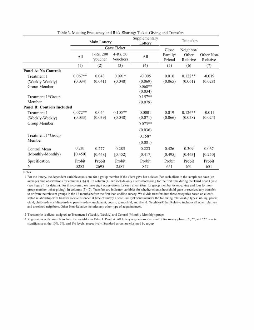
Supplementary Lottery

(1) (2) (3) (4) (5) (6) (7)Panel A: No Controls

Treatment 1 0.067** 0.043 0.091* -0.005 0.016 0.122** -0.019(Weekly-Weekly) (0.034) (0.041) (0.048) (0.069) (0.065) (0.061) (0.028)Group Member 0.068**

(0.034)0.157**(0.079)

Panel B: Controls IncludedTreatment 1 0.072** 0.044 0.105** 0.0001 0.019 0.126** -0.011(Weekly-Weekly) (0.033) (0.039) (0.048) (0.071) (0.066) (0.058) (0.024)Group Member 0.073**

(0.036)0.158*(0.081)

0.281 0.277 0.285 0.223 0.426 0.309 0.067[0.450] [0.448] [0.452] [0.417] [0.495] [0.463] [0.250]

Specification Probit Probit Probit Probit Probit Probit ProbitN 5282 2695 2587 847 651 651 651

Notes

23 Regressions with controls include the variables in Table 1, Panel A. All lottery regressions also control for survey phase. * , **, and *** denote

significance at the 10%, 5%, and 1% levels, respectively. Standard errors are clustered by group.

The sample is clients assigned to Treatment 1 (Weekly-Weekly) and Control (Monthly-Monthly) groups.

Other Non-Relative

4-Rs. 50 VouchersAll 1-Rs. 200

Voucher

1 For the lottery, the dependent variable equals one for a group member if the client gave her a ticket. For each client in the sample we have (on average) nine observations for columns (1)-(3). In column (4), we include only clients borrowing for the first time during the Third Loan Cycle (see Figure 1 for details). For this column, we have eight observations for each client (four for group member ticket-giving and four for non-group member ticket-giving). In columns (5)-(7), Transfers are indicator variables for whether client's household gave or received any transfers to or from the relevant groups in the 12 months before the first loan endline survey. We divide transfers into three categories based on client's stated relationship with transfer recipient/sender at time of survey. Close Family/Friend includes the following relationship types: sibling, parent, child, child-in-law, sibling-in-law, parent-in-law, uncle/aunt, cousin, grandchild, and friend. Neighbor/Other Relative includes all other relatives and unrelated neighbors. Other Non-Relative includes any other type of acquaintances.

Treatment 1*Group Member

Table 3. Meeting Frequency and Risk-Sharing: Ticket-Giving and Transfers

Gave TicketMain Lottery

Neighbor/ Other

Relative

Control Mean (Monthly-Monthly)

All

Transfers

Close Family/ Friend

Treatment 1*Group Member

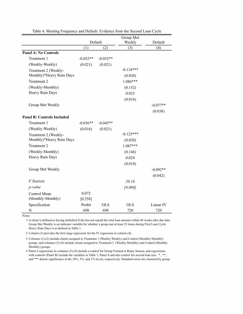
Group Met Weekly

(1) (2) (3) (4)Panel A: No Controls

Treatment 1 -0.052** -0.052**(Weekly-Weekly) (0.021) (0.021)

-0.118***(0.020)

Treatment 2 1.086***(Weekly-Monthly) (0.152)Heavy Rain Days 0.025

(0.016)Group Met Weekly -0.077**

(0.038)Panel B: Controls Included

Treatment 1 -0.036** -0.045**(Weekly-Weekly) (0.016) (0.021)

-0.125***(0.020)

Treatment 2 1.087***(Weekly-Monthly) (0.146)Heavy Rain Days 0.024

(0.018)Group Met Weekly -0.092**

(0.042)F Statistic 20.16p-value [0.000]

0.072[0.258]

Specification Probit OLS OLS Linear IVN 698 698 720 720

Notes

2

3

4

Treatment 2 (Weekly-Monthly)*Heavy Rain Days

Treatment 2 (Weekly-Monthly)*Heavy Rain Days

Control Mean (Monthly-Monthly)

Default

Columns (1)-(2) include clients assigned to Treatment 1 (Weekly-Weekly) and Control (Monthly-Monthly) groups, and columns (3)-(4) include clients assigned to Treatment 2 (Weekly-Monthly) and Control (Monthly-Monthly) groups.

Table 4. Meeting Frequency and Default: Evidence from the Second Loan Cycle

A client is defined as having defaulted if she has not repaid the total loan amount within 44 weeks after due date. Group Met Weekly is an indicator variable for whether a group met at least 23 times during First Loan Cycle. Heavy Rain Days is as defined in Table 1.Column (3) provides the first stage regression for the IV regression in column (4).

Panel A regressions in columns (3)-(4) include a control for Group Formed in Rainy Season, and regressions with controls (Panel B) include the variables in Table 1, Panel A and also control for second loan size. * , **, and *** denote significance at the 10%, 5%, and 1% levels, respectively. Standard errors are clustered by group.

1

Default

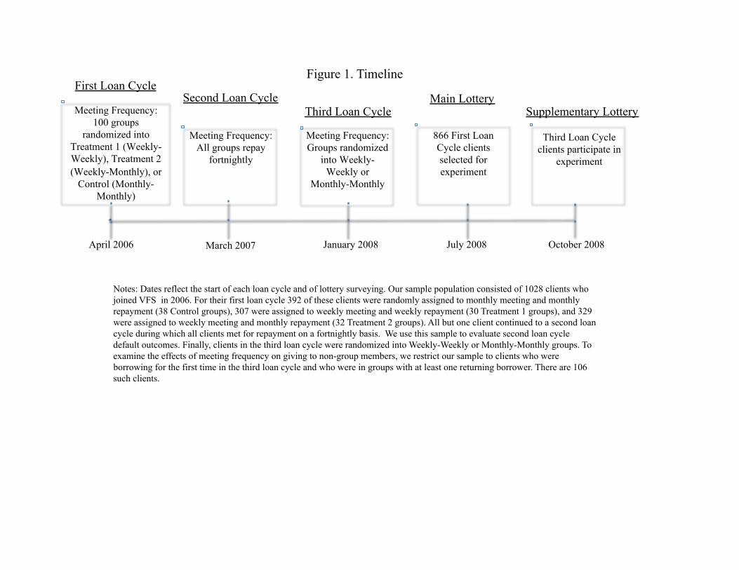
Figure 1. Timeline

Notes: Dates reflect the start of each loan cycle and of lottery surveying. Our sample population consisted of 1028 clients who joined VFS in 2006. For their first loan cycle 392 of these clients were randomly assigned to monthly meeting and monthly repayment (38 Control groups), 307 were assigned to weekly meeting and weekly repayment (30 Treatment 1 groups), and 329 were assigned to weekly meeting and monthly repayment (32 Treatment 2 groups). All but one client continued to a second loan cycle during which all clients met for repayment on a fortnightly basis. We use this sample to evaluate second loan cycle default outcomes. Finally, clients in the third loan cycle were randomized into Weekly-Weekly or Monthly-Monthly groups. To examine the effects of meeting frequency on giving to non-group members, we restrict our sample to clients who were borrowing for the first time in the third loan cycle and who were in groups with at least one returning borrower. There are 106 such clients.

April 2006

Meeting Frequency: 100 groups

randomized into Treatment 1 (Weekly-Weekly), Treatment 2 (Weekly-Monthly), or

Control (Monthly-Monthly)

March 2007

January 2008 July 2008

Meeting Frequency: All groups repay

fortnightly

866 First Loan Cycle clients selected for experiment

Meeting Frequency: Groups randomized

into Weekly-Weekly or

Monthly-Monthly

First Loan Cycle Second Loan Cycle Main Lottery

Third Loan Cycle Supplementary Lottery

October 2008

Third Loan Cycle clients participate in

experiment

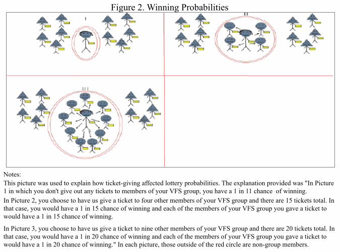
Notes:

Figure 2. Winning Probabilities

This picture was used to explain how ticket-giving affected lottery probabilities. The explanation provided was "In Picture 1 in which you don't give out any tickets to members of your VFS group, you have a 1 in 11 chance of winning. In Picture 2, you choose to have us give a ticket to four other members of your VFS group and there are 15 tickets total. In that case, you would have a 1 in 15 chance of winning and each of the members of your VFS group you gave a ticket to would have a 1 in 15 chance of winning.

In Picture 3, you choose to have us give a ticket to nine other members of your VFS group and there are 20 tickets total. In that case, you would have a 1 in 20 chance of winning and each of the members of your VFS group you gave a ticket to would have a 1 in 20 chance of winning." In each picture, those outside of the red circle are non-group members.

0.5

11.

52

Den

sity

0 .2 .4 .6 .8 1Fraction of Group Members Given Ticket

Treatment 1 (Weekly-Weekly)Treatment 2 (Weekly-Monthly)Control (Monthly-Monthly)

Figure 3: Client-Level Distribution of Ticket-Giving

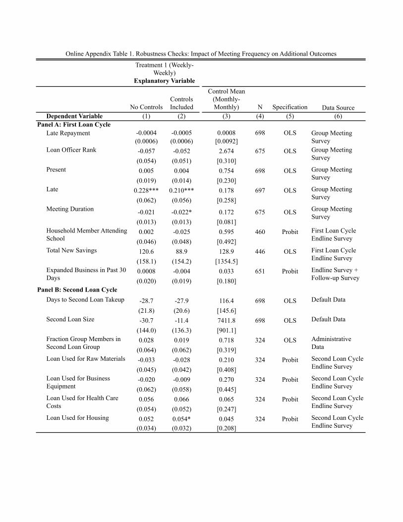
No ControlsControls Included

Control Mean (Monthly-Monthly) N Specification Data Source

Dependent Variable (1) (2) (3) (4) (5) (6)Panel A: First Loan Cycle

-0.0004 -0.0005 0.0008 698 OLS(0.0006) (0.0006) [0.0092]-0.057 -0.052 2.674 675 OLS(0.054) (0.051) [0.310]0.005 0.004 0.754 698 OLS

(0.019) (0.014) [0.230]0.228*** 0.210*** 0.178 697 OLS(0.062) (0.056) [0.258]

-0.021 -0.022* 0.172 675 OLS(0.013) (0.013) [0.081]0.002 -0.025 0.595 460 Probit

(0.046) (0.048) [0.492]120.6 88.9 128.9 446 OLS

(158.1) (154.2) [1354.5]0.0008 -0.004 0.033 651 Probit(0.020) (0.019) [0.180]

Panel B: Second Loan Cycle

-28.7 -27.9 116.4 698 OLS(21.8) (20.6) [145.6]-30.7 -11.4 7411.8 698 OLS

(144.0) (136.3) [901.1]0.028 0.019 0.718 324 OLS

(0.064) (0.062) [0.319]-0.033 -0.028 0.210 324 Probit(0.045) (0.042) [0.408]-0.020 -0.009 0.270 324 Probit(0.062) (0.058) [0.445]0.056 0.066 0.065 324 Probit

(0.054) (0.052) [0.247]Loan Used for Housing 0.052 0.054* 0.045 324 Probit

(0.034) (0.032) [0.208]

Household Member Attending School

Days to Second Loan Takeup

Meeting Duration

Late

Total New Savings

Expanded Business in Past 30 Days

Loan Used for Raw Materials

Loan Used for Business Equipment

Late Repayment

Loan Officer Rank

Present

Second Loan Size

Fraction Group Members in Second Loan Group

Group Meeting SurveyGroup Meeting Survey

Group Meeting Survey

Group Meeting Survey

Group Meeting Survey

Online Appendix Table 1. Robustness Checks: Impact of Meeting Frequency on Additional Outcomes

Treatment 1 (Weekly-Weekly)

Explanatory Variable

First Loan Cycle Endline Survey

Endline Survey + Follow-up Survey

First Loan Cycle Endline Survey

Default Data

Default Data

Administrative Data

Second Loan Cycle Endline Survey

Second Loan Cycle Endline Survey

Second Loan Cycle Endline Survey

Second Loan Cycle Endline Survey

Loan Used for Health Care Costs

Notes

2

34

1

The sample is clients assigned to Treatment 1 (Weekly-Weekly) and Control (Monthly-Monthly) groups.Regressions with controls include the variables in Table 1, Panel A (except for Days to Second Loan Takeup specification which includes all controls except for Group Formed in Rainy Season). * , **, and *** denote significance at the 10%, 5%, and 1% levels, respectively. Standard errors are clustered by group.

Late Repayment is the fraction of group meetings at which a client failed to make the scheduled repayment. Loan Officer Rank is measured on a four-point scale, with higher rankings reflecting a higher perceived ability to repay. Present and Late are averages taken for group meetings between week 9 and week 23 of the loan cycle. Meeting Duration is measured in hours and is averaged across all group meetings. Days to Second Loan Takeup is defined as the number of days between scheduled First Loan repayment and Second Loan takeup. Fraction Group Members in Second Loan Group is defined as the fraction of second loan group members also in first loan group. Loan Used for _______ are indicator variables and multiple loan uses may be listed for each loan in Second Loan Cycle. For First Loan Cycle questions on savings and school attendance, the sample excludes First Loan Cycle clients who received the follow-up survey (which did not ask about these topics and was administered to clients who repaid their initial loans faster than anticipated). For Second Loan Cycle loan use questions, the sample includes only First Loan Cycle clients who remained research clients during the Second Loan Cycle (and so continued to be surveyed regarding loan use).

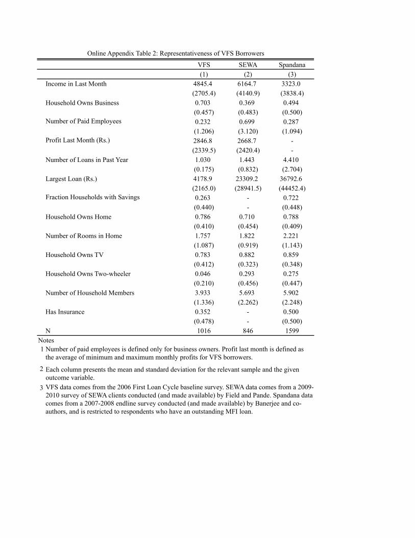
VFS SEWA Spandana(1) (2) (3)

Income in Last Month 4845.4 6164.7 3323.0(2705.4) (4140.9) (3838.4)

Household Owns Business 0.703 0.369 0.494(0.457) (0.483) (0.500)

Number of Paid Employees 0.232 0.699 0.287(1.206) (3.120) (1.094)

Profit Last Month (Rs.) 2846.8 2668.7 -(2339.5) (2420.4) -

Number of Loans in Past Year 1.030 1.443 4.410(0.175) (0.832) (2.704)

Largest Loan (Rs.) 4178.9 23309.2 36792.6(2165.0) (28941.5) (44452.4)

Fraction Households with Savings 0.263 - 0.722(0.440) - (0.448)

Household Owns Home 0.786 0.710 0.788(0.410) (0.454) (0.409)

Number of Rooms in Home 1.757 1.822 2.221(1.087) (0.919) (1.143)

Household Owns TV 0.783 0.882 0.859(0.412) (0.323) (0.348)

Household Owns Two-wheeler 0.046 0.293 0.275(0.210) (0.456) (0.447)

Number of Household Members 3.933 5.693 5.902(1.336) (2.262) (2.248)

Has Insurance 0.352 - 0.500(0.478) - (0.500)

N 1016 846 1599Notes1

2

3

Online Appendix Table 2: Representativeness of VFS Borrowers

Number of paid employees is defined only for business owners. Profit last month is defined as the average of minimum and maximum monthly profits for VFS borrowers.

Each column presents the mean and standard deviation for the relevant sample and the given outcome variable.VFS data comes from the 2006 First Loan Cycle baseline survey. SEWA data comes from a 2009-2010 survey of SEWA clients conducted (and made available) by Field and Pande. Spandana data comes from a 2007-2008 endline survey conducted (and made available) by Banerjee and co-authors, and is restricted to respondents who have an outstanding MFI loan.

Received Baseline Survey

Received Endline Survey

(1) (2)Panel A: No Controls

Treatment 1 0.015* 0.035(Weekly-Weekly) (0.008) (0.023)Treatment 2 0.006 0.026(Weekly-Monthly) (0.010) (0.021)

0.982 0.916[0.133] [0.278]

Specification OLS OLSN 1028 1028

Notes

Control Mean (Monthly-Monthly)

1 * , **, and *** denote significance at the 10%, 5%, and 1% levels, respectively. Standard errors are clustered by group.

Online Appendix Table 3. Survey Attrition

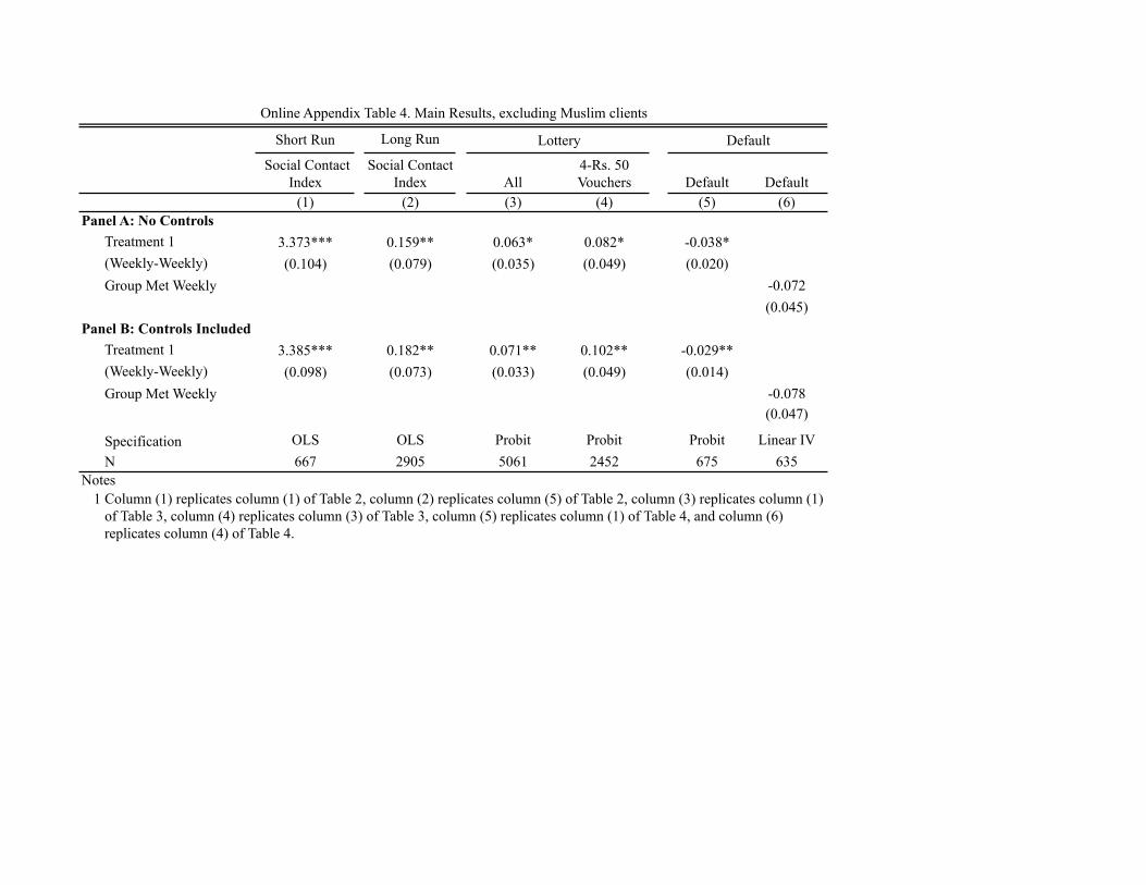
Short Run Long Run

Social Contact Index

Social Contact Index All

4-Rs. 50 Vouchers Default Default

(1) (2) (3) (4) (5) (6)Panel A: No Controls

Treatment 1 3.373*** 0.159** 0.063* 0.082* -0.038*(Weekly-Weekly) (0.104) (0.079) (0.035) (0.049) (0.020)Group Met Weekly -0.072

(0.045)Panel B: Controls Included

Treatment 1 3.385*** 0.182** 0.071** 0.102** -0.029**(Weekly-Weekly) (0.098) (0.073) (0.033) (0.049) (0.014)Group Met Weekly -0.078

(0.047)

Specification OLS OLS Probit Probit Probit Linear IVN 667 2905 5061 2452 675 635

Notes

Lottery Default

1 Column (1) replicates column (1) of Table 2, column (2) replicates column (5) of Table 2, column (3) replicates column (1) of Table 3, column (4) replicates column (3) of Table 3, column (5) replicates column (1) of Table 4, and column (6) replicates column (4) of Table 4.

Online Appendix Table 4. Main Results, excluding Muslim clients

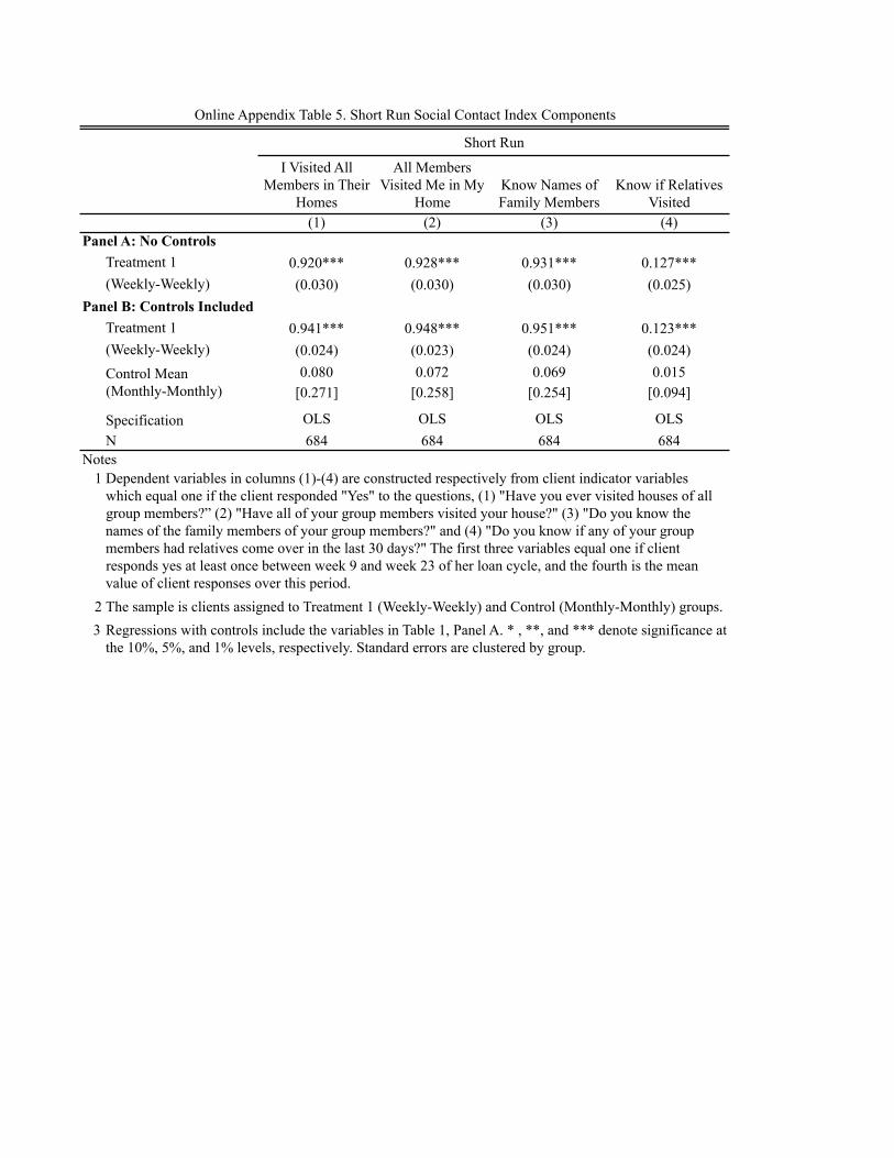
I Visited AllMembers in Their

Homes

All MembersVisited Me in My

HomeKnow Names ofFamily Members

Know if RelativesVisited

(1) (2) (3) (4)Panel A: No Controls

Treatment 1 0.920*** 0.928*** 0.931*** 0.127***(Weekly-Weekly) (0.030) (0.030) (0.030) (0.025)

Panel B: Controls IncludedTreatment 1 0.941*** 0.948*** 0.951*** 0.123***(Weekly-Weekly) (0.024) (0.023) (0.024) (0.024)

0.080 0.072 0.069 0.015[0.271] [0.258] [0.254] [0.094]

Specification OLS OLS OLS OLSN 684 684 684 684

Notes

23 Regressions with controls include the variables in Table 1, Panel A. * , **, and *** denote significance at

the 10%, 5%, and 1% levels, respectively. Standard errors are clustered by group.

Control Mean (Monthly-Monthly)

1 Dependent variables in columns (1)-(4) are constructed respectively from client indicator variables which equal one if the client responded "Yes" to the questions, (1) "Have you ever visited houses of all group members?” (2) "Have all of your group members visited your house?" (3) "Do you know the names of the family members of your group members?" and (4) "Do you know if any of your group members had relatives come over in the last 30 days?" The first three variables equal one if client responds yes at least once between week 9 and week 23 of her loan cycle, and the fourth is the mean value of client responses over this period. The sample is clients assigned to Treatment 1 (Weekly-Weekly) and Control (Monthly-Monthly) groups.

Online Appendix Table 5. Short Run Social Contact Index Components

Short Run

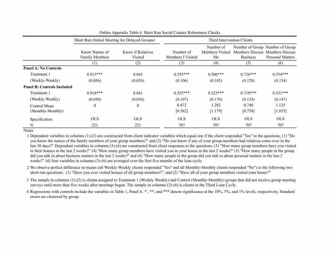
Know Names ofFamily Members

Know if RelativesVisited

Number of Members I Visited

Number of Members Visited

Me

Number of Group Members Discuss

Business

Number of Group Members Discuss Personal Matters

(1) (2) (3) (4) (5) (6)Panel A: No Controls

Treatment 1 0.913*** 0.043 0.555*** 0.506*** 0.726*** 0.534***(Weekly-Weekly) (0.056) (0.039) (0.106) (0.183) (0.128) (0.154)

Panel B: Controls IncludedTreatment 1 0.918*** 0.041 0.555*** 0.525*** 0.719*** 0.531***(Weekly-Weekly) (0.050) (0.036) (0.107) (0.170) (0.124) (0.147)

0 0 0.472 1.282 0.740 1.125. . [0.562] [1.179] [0.758] [1.035]

Specification OLS OLS OLS OLS OLS OLSN 221 221 707 707 707 707

Notes

2

3

4

1

Control Mean (Monthly-Monthly)

Dependent variables in columns (1)-(2) are constructed from client indicator variables which equal one if the client responded "Yes" to the questions, (1) "Do you know the names of the family members of your group members?" and (2) "Do you know if any of your group members had relatives come over in the last 30 days?" Dependent variables in columns (3)-(6) are constructed from client responses to the questions, (3) "How many group members have you visited in their houses in the last 2 weeks?” (4) "How many group members have visited you in your house in the last 2 weeks?" (5) "How many people in the group did you talk to about business matters in the last 2 weeks?" and (6) "How many people in the group did you talk to about personal matters in the last 2 weeks?" All four variables in columns (3)-(6) are averaged over the first five months of the loan cycle.

The sample in columns (1)-(2) is clients assigned to Treatment 1 (Weekly-Weekly) and Control (Monthly-Monthly) groups that did not receive group meeting surveys until more than five weeks after meetings began. The sample in columns (3)-(6) is clients in the Third Loan Cycle.Regressions with controls include the variables in Table 1, Panel A. * , **, and *** denote significance at the 10%, 5%, and 1% levels, respectively. Standard errors are clustered by group.

We observe perfect difference in means (all Weekly-Weekly clients responded "Yes" and all Monthly-Monthly clients responded "No") to the following two short-run questions: (1) "Have you ever visited houses of all group members?”, and (2) "Have all of your group members visited your house?"

Online Appendix Table 6. Short Run Social Contact Robustness Checks

Short Run (Initial Meeting for Delayed Groups) Third Intervention Clients

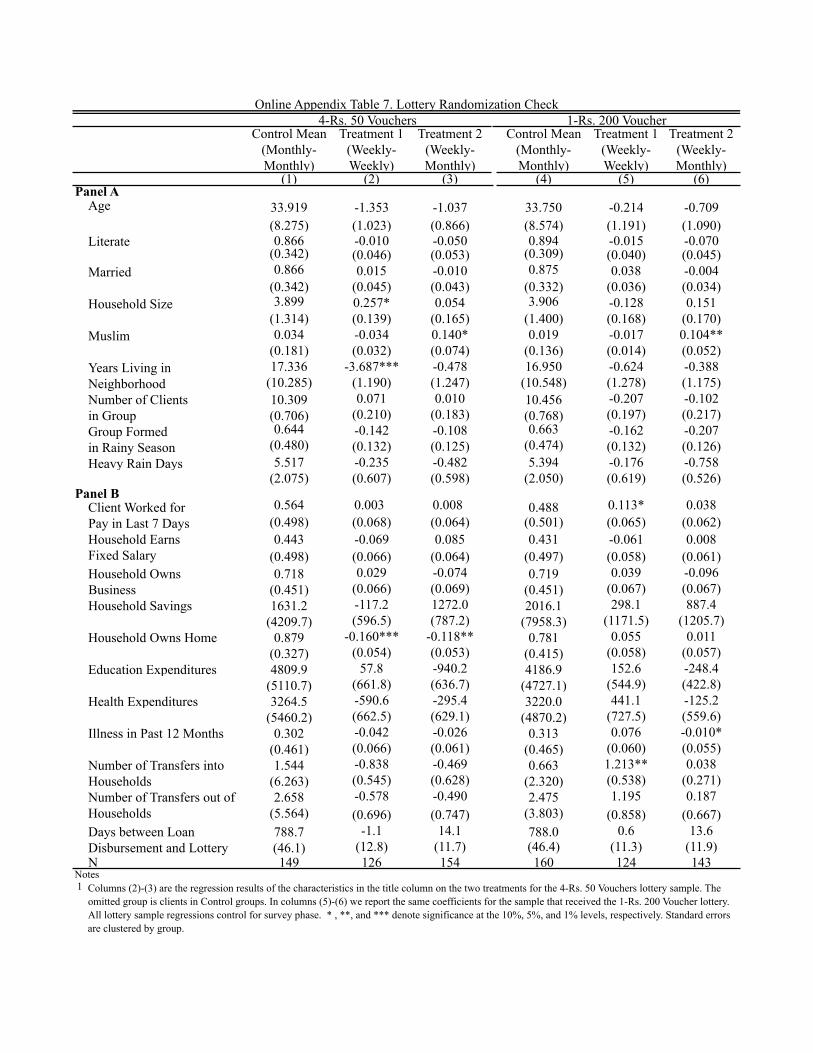
Control Mean (Monthly-Monthly)

Treatment 1 (Weekly-Weekly)

Treatment 2 (Weekly-Monthly)

Control Mean (Monthly-Monthly)

Treatment 1 (Weekly-Weekly)

Treatment 2 (Weekly-Monthly)

(1) (2) (3) (4) (5) (6)Panel A

Age 33.919 -1.353 -1.037 33.750 -0.214 -0.709(8.275) (1.023) (0.866) (8.574) (1.191) (1.090)

Literate 0.866 -0.010 -0.050 0.894 -0.015 -0.070(0.342) (0.046) (0.053) (0.309) (0.040) (0.045)

Married 0.866 0.015 -0.010 0.875 0.038 -0.004(0.342) (0.045) (0.043) (0.332) (0.036) (0.034)

Household Size 3.899 0.257* 0.054 3.906 -0.128 0.151(1.314) (0.139) (0.165) (1.400) (0.168) (0.170)

Muslim 0.034 -0.034 0.140* 0.019 -0.017 0.104**(0.181) (0.032) (0.074) (0.136) (0.014) (0.052)17.336 -3.687*** -0.478 16.950 -0.624 -0.388

(10.285) (1.190) (1.247) (10.548) (1.278) (1.175)10.309 0.071 0.010 10.456 -0.207 -0.102(0.706) (0.210) (0.183) (0.768) (0.197) (0.217)0.644 -0.142 -0.108 0.663 -0.162 -0.207

(0.480) (0.132) (0.125) (0.474) (0.132) (0.126)Heavy Rain Days 5.517 -0.235 -0.482 5.394 -0.176 -0.758

(2.075) (0.607) (0.598) (2.050) (0.619) (0.526)

0.564 0.003 0.008 0.488 0.113* 0.038(0.498) (0.068) (0.064) (0.501) (0.065) (0.062)0.443 -0.069 0.085 0.431 -0.061 0.008

(0.498) (0.066) (0.064) (0.497) (0.058) (0.061)0.718 0.029 -0.074 0.719 0.039 -0.096

(0.451) (0.066) (0.069) (0.451) (0.067) (0.067)Household Savings 1631.2 -117.2 1272.0 2016.1 298.1 887.4

(4209.7) (596.5) (787.2) (7958.3) (1171.5) (1205.7)Household Owns Home 0.879 -0.160*** -0.118** 0.781 0.055 0.011

(0.327) (0.054) (0.053) (0.415) (0.058) (0.057)Education Expenditures 4809.9 57.8 -940.2 4186.9 152.6 -248.4

(5110.7) (661.8) (636.7) (4727.1) (544.9) (422.8)Health Expenditures 3264.5 -590.6 -295.4 3220.0 441.1 -125.2

(5460.2) (662.5) (629.1) (4870.2) (727.5) (559.6)0.302 -0.042 -0.026 0.313 0.076 -0.010*

(0.461) (0.066) (0.061) (0.465) (0.060) (0.055)1.544 -0.838 -0.469 0.663 1.213** 0.038

(6.263) (0.545) (0.628) (2.320) (0.538) (0.271)2.658 -0.578 -0.490 2.475 1.195 0.187

(5.564) (0.696) (0.747) (3.803) (0.858) (0.667)788.7 -1.1 14.1 788.0 0.6 13.6(46.1) (12.8) (11.7) (46.4) (11.3) (11.9)

N 149 126 154 160 124 143Notes1 Columns (2)-(3) are the regression results of the characteristics in the title column on the two treatments for the 4-Rs. 50 Vouchers lottery sample. The

omitted group is clients in Control groups. In columns (5)-(6) we report the same coefficients for the sample that received the 1-Rs. 200 Voucher lottery. All lottery sample regressions control for survey phase. * , **, and *** denote significance at the 10%, 5%, and 1% levels, respectively. Standard errors are clustered by group.

Number of Transfers out of HouseholdsDays between Loan Disbursement and Lottery

Panel BClient Worked for Pay in Last 7 DaysHousehold Earns Fixed Salary Household Owns Business

Illness in Past 12 Months

Number of Transfers into Households

Number of Clients in GroupGroup Formed in Rainy Season

Years Living in Neighborhood

Online Appendix Table 7. Lottery Randomization Check4-Rs. 50 Vouchers 1-Rs. 200 Voucher

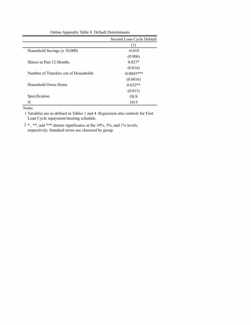
Second Loan Cycle Default(1)

Household Savings (x 10,000) -0.010(0.006)

Illness in Past 12 Months 0.027*(0.016)

Number of Transfers out of Households -0.0043***(0.0016)

Household Owns Home 0.032**(0.015)

Specification OLSN 1015

Notes1

2

Online Appendix Table 8. Default Determinants

Variables are as defined in Tables 1 and 4. Regression also controls for First Loan Cycle repayment/meeting schedule.

* , **, and *** denote significance at the 10%, 5%, and 1% levels, respectively. Standard errors are clustered by group.

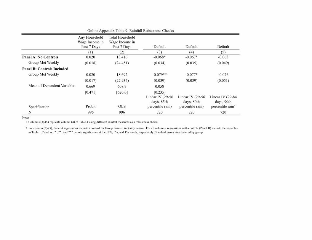
Any Household Wage Income in

Past 7 Days

Total Household Wage Income in

Past 7 Days Default Default Default(1) (2) (3) (4) (5)

Panel A: No Controls 0.020 18.416 -0.068* -0.067* -0.063Group Met Weekly (0.018) (24.451) (0.034) (0.035) (0.049)

Panel B: Controls IncludedGroup Met Weekly 0.020 18.692 -0.079** -0.077* -0.076

(0.017) (22.934) (0.039) (0.039) (0.051)0.669 608.9 0.058

[0.471] [620.0] [0.235]

Specification Probit OLS

Linear IV (29-56 days, 85th

percentile rain)

Linear IV (29-56 days, 80th

percentile rain)

Linear IV (29-84 days, 90th

percentile rain)N 996 996 720 720 720

Notes

2 For column (3)-(5), Panel A regressions include a control for Group Formed in Rainy Season. For all columns, regressions with controls (Panel B) include the variables in Table 1, Panel A. * , **, and *** denote significance at the 10%, 5%, and 1% levels, respectively. Standard errors are clustered by group.

1 Columns (3)-(5) replicate column (4) of Table 4 using different rainfall measures as a robustness check.

Online Appendix Table 9. Rainfall Robustness Checks

Mean of Dependent Variable

Note:

Appendix Figure 1. Lottery Vouchers

Clients were randomly offered entry into the lottery for a Rs. 200 Voucher or four Rs. 50 Vouchers. This figure shows the final vouchers which were given to the winner of the two lotteries.

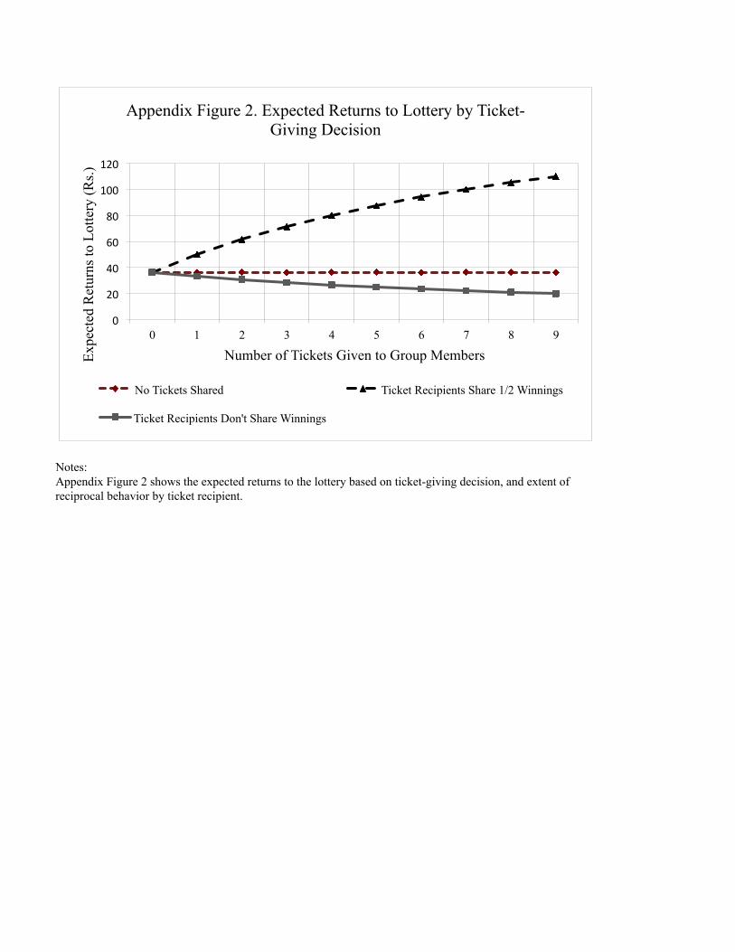
0.4282 00.1111 10.088 2

0.0926 30.1181 40.0486 50.0162 60.0255 70.0185 80.0532 9

Notes: Appendix Figure 2 shows the expected returns to the lottery based on ticket-giving decision, and extent of reciprocal behavior by ticket recipient.

0  

20  

40  

60  

80  

100  

120  

0 1 2 3 4 5 6 7 8 9

Expe

cted

Ret

urns

to L

otte

ry (R

s.)

Number of Tickets Given to Group Members

Appendix Figure 2. Expected Returns to Lottery by Ticket-Giving Decision

No Tickets Shared Ticket Recipients Share 1/2 Winnings

Ticket Recipients Don't Share Winnings

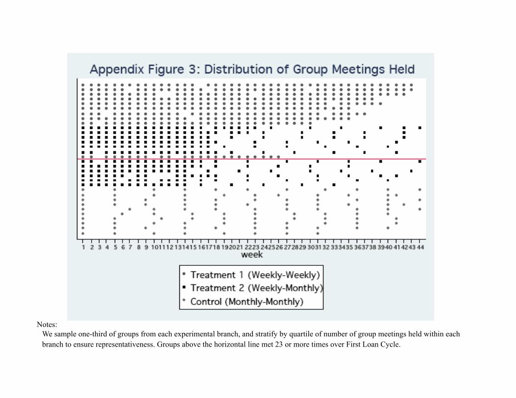
Notes:We sample one-third of groups from each experimental branch, and stratify by quartile of number of group meetings held within each branch to ensure representativeness. Groups above the horizontal line met 23 or more times over First Loan Cycle.