energy or mass and interaction - prof.usb.veprof.usb.ve/ggonzalm/invstg/pblc/enrgymssint.pdf ·...
TRANSCRIPT

EnerEnerEnerEnerEnergggggy or Massy or Massy or Massy or Massy or Massand Interactionand Interactionand Interactionand Interactionand Interaction

ii
iii
Energy or Mass and
Interaction
Gustavo R. González-Martín
Professor, Physics Department
Simón Bolívar University
Caracas

iv
First English Edition, first published in 2010
© Gustavo R. González-Martín 2010
An abridged english translation of “Geometría Fisica”,© Gustavo R. González Martín 1999, 2010Abridged and translated from the Spanishby the author.
Departamento de FísicaUniversidad Simón BolívarValle de Sartenejas, Baruta, Estado MirandaApartado 89000, Caracas 1080-A, Venezuela

v
…Mach felt that there was something important about this concept of avoidingan inertial system… Not yet so clear in Riemann’s concept of space. The first tosee this clearly was Levi-Civita: absolute parallelism and a way to differentiate…
…The representation of matter by a tensor was only a fill-in to make it possibleto do something temporarily, a wooden nose in a snowman…
…For most people, special relativity, electromagnetism and gravitation areunimportant, to be added in at the end after everything else has been done. Onthe contrary, we have to take them into account from the beginning…
Albert Einstein
from Albert Einstein’s Last Lecture,3
Relativity Seminar,Room 307, Palmer Physical Laboratory, Princeton University,April 14, 1954,according to notes taken by J. A. Wheeler.
3 J. A. Wheeler in: P. C. Eichelburg and R. U. Sexl (Eds.), Albert Einstein (Friedr. Vieweg & Sohn, Braunschweig) p. 201, (1979).

vi

vii
PrefaceThe physical ideas previously presented in Physical Geometry are published in cited
scientific journals. Nevertheless some of our latest numerical results, which are availableas e-prints at www.arXiv.org, have met resistance to publication by certain journals. Thisseems to be a reflection of opinions held by some groups involved in research along somepresently canonical particle lines. These lines introduce models, in terms of either a largenumber of dimensions or a very large number of empirical parameters, which are not clearlyrelated to a fundamental underlying theoretical physical interaction.
Our ideas represent a critique of these models and indicate the need of a researchthrust along a new direction. In this regard, the following general aspects should bepointed out: In first place, we have presented many new numerical results which are notcalculable from known physical models; In second place, these numbers arise from theconcept of energy and a generalized nonlinear electrodynamics, whose QFT should beused for perturbations corrections; In third place, there appears to be no physical experi-mental evidence contradicting our ideas. We also appreciate that there are difficultiesunderstanding the results obtained in our work because we presented them in a geometri-cally unified form. The essential objective is to start from geometry, which represents formand has developed from observations of the universe during more that 25 centuries.
For these reasons there is a need to discuss these physical-geometric ideas withoutthe burden of a complete mathematical treatment. Therefore, in this abridged book wemake emphasis on physical aspects of the theory, in particular at the start of each chapter.To help the reader a brief summary of the results is presented at the end of chapters.
In particular, here we discus the following: 1- The connection between energy andnumerical masses; 2- The energy-mass classification of particles as fundamental represen-tations of a relativity group action; 3- The unification of interactions, in particular theidentification of short-distance nuclear effects with a fundamental electromagnetic su(2)subinteraction which provides very strong short-range attractive magnetic potentials andenergy and predicts experimental nuclear data; 4- The existence of energy-mass terms in ageneralized Einstein equation which appear to lead to dark matter and energy; 5- The needand relevance of classical statistics in a theory of microscopic measurements.
Caracas, Venezuela, February 24, 2010. Gustavo R. González Martín
Preface to Physical GeometryThe objective is to establish a foundations for unification of physical forces in order to
give answers to fundamental questions: What are the relations among the concepts ofenergy, mass, inertia and interaction forces? The fundamental ideas and results arepublished in the references.
It is recognized that the action of matter defines these concepts and their relations, allof them capable of geometrical representation. The main aspects of the theory are thefollowing:
1. The physical universe is described by matter equations associated to anevolution group.
2. The group is obtained from geometric algebraic tranformations of space andtime.
3. The interaction is represented by field equations and equations of motion in

viii
terms of potential and force tensors determined by matter transformationcurrents.
4. Microscopic physics is seen as the study of linear geometric excitations, whichare representations of the group, characterized by a set of discrete numbers.
5. The equations determine fundamental concepts of energy, mass and inertiawhich classify the interactions and particles.
The results obtained indicate that gravitation and electromagnetism are unifiedin a nontrivial manner. There are additional generators that may represent non classicalinteractions. Multipole equations of motion determine the geodesic motion with the Lorentzforce term. If we restrict to the even part, we obtain the Einstein field equation and a purelygeometric energy momentum tensor that indicate the possibility of a geometric internalsolution. The constant curvature parameter (geometric energy density) of a hyperbolicsymmetric solution may be related, in the newtonian limit, to the gravitational constant G.If the nonriemannian connection fields contribute to the scalar curvature, the parameter Gwould be variable, diminishing with the field intensity. This effect may be interpreted asthe presence of dark matter or energy. In vacuum, the known gravitational solutions witha cosmological constant are obtained. Electromagnetism is related to an SU(2)Q subgroup.If we exclusively restrict to a U(1) subgroup we obtain Maxwell’s field equations. Ingeneral, the equation of motion is a geometric generalization of Dirac’s equation. In fact,it appears that this geometry is the germ of quantum physics including its probabilisticaspects. The geometric nature of Planck’s constant h and of light speed c is determined bytheir respective relations to the connection and the metric. The mass is defined in aninvariant manner in terms of energy, depending on the connection and matter frames.The geometry shows a triple structure that determines various physical triple structures.The geometric excitations have quanta of charge, flux and spin that determine the fractionalquantum Hall effect. The quotient of bare masses of the three stable particles are calculatedand leads us to a surprising geometric expression for the proton electron mass ratio,previously known but physically unexplained. There are massive connection excitationswhose masses correspond to the weak boson masses and allow a geometric interpretationof Weinberg’s angle.The geometric equation of motion (a generalized Dirac equation)determines the anomalous bare magnetic moments of the proton, the electron and theneutron. The “strong” electromagnetic SU(2)Q part, without the help of any other force,generates nuclear range attractive potentials which are sufficiently strong to determinethe binding energy of the deuteron and other light nuclides, composed of protons andelectrons. The bare masses of the leptons in the three families are calculated as topologicalexcitations of the electron. The masses of these excitations increase under the action of astrong connection (relativity of energy) and are related to meson masses. The geometrydetermines the geometric excitation mass spectrum, which for low masses, essentiallyagrees with the physical particle mass spectrum. The proton shows a triple structure thatmay be related to a quark structure. The combinations of the three fundamental geometricexcitations (associated to the proton, the electron and the neutrino), forming otherexcitations, may be used to represent particles and show a symmetry under the groupSU(3)SU(2)U(1). The alpha coupling constant is also determined geometrically.
The first two chapters represent an introduction. In chapters 3 to 10 the fundamentalgeometric ideas are developed. In chapters 11 to 18 the theory is applied to concrete cases.
Caracas, Venezuela, February 24, 2010. Gustavo R. González Martín

ix
q 1
q 2
q 3EQ
E E iE- = 1 2
E E+ = 3
“The odd -E generators determine attractive, short-range potentialswhich are sufficiently strong to sustain nuclear fusion.”
A geometric universal action?Are neutron stars natural laboratories for these energy processes?
Geometric Quantization of theSU(2) electromagnetic potentialand the electric charge.

x

xi
To Lourdes

xii
Acknowledgments
I have tried to give credit to those whose work give support to the ideasexpressed in this book. Nevertheless, it appears impossible to accomplish thiscompletely. At the moment of writing, it is much what I owe to those from which Ihave learned throughout the years. In this sense, I am grateful to the membersphysics community of the Boston area, in particular to my professor, John Stachel.
Specially I want to thank the colleagues with whom I discussed these topics,even if I am unable to precisely determine the contribution to the germination andformation of the ideas; in particular, the senior faculty of the Caracas Relativityand Fields Seminar: Luis Herrera Cometa, Alvaro Restuccia, Sebastián Salamó andCarlos Aragone (R.I.P.). I also acknowledge the collaboration of research assis-tants and some students in my relativity courses and special lectures on unifica-tion at the Simón Bolívar University, who served as stimulating test in the presen-tation and discussion of the geometric hypothesis of physics: G. Salas, G. Sarmiento,V. Villalba, V. Varela, A. Mendoza, O. Rendón, E. Valdeblánquez, I. Taboada, V. DiClemente, J. Díaz, J. González T., A. de Castro, A. Hernández and M. A. Lledó.
Caracas, Venezuela, June 20, 2000. Gustavo R. González Martín

xiii
CONTENTS1. Energy. ............................................................................................ 1
1.1. Extension of Relativity. ................................................................................. 21.2. Energy and the Field Equation. .................................................................... 51.3. Inertial Effects and Mass. ............................................................................. 81.4. The Classical Fields. ................................................................................... 111.5. Results. ...................................................................................................... 13
2. Quanta. ......................................................................................... 142.1. Induced Representations of the Structure Group G. ................................... 142.2. Relation Among Quantum Numbers. .......................................................... 162.3. Spin, Charge and Flux. ................................................................................ 172.4. Representations of a Subgroup P. .............................................................. 192.5. Magnetic Flux Quanta. ............................................................................... 212.6. Magnetic Energy Levels. ........................................................................... 222.7. Fractional Quantum Hall Effects. ................................................................ 252.8. Results. ...................................................................................................... 27
3. Measurements and Motion. ........................................................ 283.1. Measurement of Geometric Currents. ......................................................... 293.2. Geometric Spin. .......................................................................................... 313.3. Geometric Charge. ...................................................................................... 323.4. The Concept of Mass. ................................................................................ 353.5. Invariant Mass. .......................................................................................... 363.6. Equation of Motion. ................................................................................... 38
3.6.1. Agreement with Standard Quantum Mechanics. ............................... 393.7. Results. ...................................................................................................... 42
4. Masses. ........................................................................................ 434.1. Bare Inertial Masses for Frame Excitations or Fermions. ............................ 454.2. Symmetric Cosets. ...................................................................................... 50
4.2.1. Volume of C Space. ............................................................................ 504.2.2. Volume of K space. ............................................................................ 504.2.3. Ratio of Geometric Volumes ............................................................... 51
4.3. The p, e and n Mass Ratios. ....................................................................... 524.4. The Equation for the Potential Excitations or Bosons. ............................... 524.5. Massive Particular Solutions. ..................................................................... 534.6. Massive SU(2) Bosons. .............................................................................. 55
4.6.1. Mass Values in Free Space. ............................................................... 604.6.2. Potential Excitations in a Lattice. ....................................................... 61
4.7. Results. ...................................................................................................... 625. Nuclear Energy and Interaction. ................................................. 64
5.1. Nonrelativistic Motion of an Excitation. ..................................................... 645.2. Magnetic Moments of p, e and n. .............................................................. 655.3. The Modified Pauli Equation. ..................................................................... 695.4. The Proton-Electron-Proton Model for the Deuteron. ............................... 71
xiv
5.5. Binding Energy of the Deuteron. ............................................................... 745.6. The Electron-Proton Model for the Neutron. ............................................. 765.7. The Many Deuteron Model. ...................................................................... 77
5.7.1. Nuclear Structure, Fusion and Fission. ............................................. 795.8. Geometric Weak Interations. ...................................................................... 805.9. Relation with Fermi’s Theory. ..................................................................... 835.10. Results. ...................................................................................................... 86
6. Particles and Interactions. ........................................................... 876.1. Geometric Classification of the Potential. ................................................... 876.2. Algebraic Structure of Particles. ................................................................. 886.3. Interpretation as Particles and Interactions. ............................................... 916.4. Topological Structure of Particles. ............................................................. 926.5. Geometric Excitation Masses. ..................................................................... 94
6.5.1. Leptonic Masses. .............................................................................. 966.5.2. Mesonic Masses. .............................................................................. 98
6.6. Barut’s Model. .......................................................................................... 1026.7. Relation with Particle Theory. ................................................................... 1066.8. Results. .................................................................................................... 108
7. Gravitation and Geometry. ........................................................ 1097.1. Einstein’s Equation. .................................................................................. 109
7.1.1. Newtonian G and the Schwarzschild Mass. .................................... 1127.2. Dark Matter Effects. ................................................................................. 1157.3. The Alpha Constant. ................................................................................ 116
7.3.1. Symmetric Space K. ......................................................................... 1177.3.2. Wyler’s Measure on the K Space. ................................................... 1177.3.3. Value of the Geometric Coefficient. ................................................. 118
7.4. Results. .................................................................................................... 1198. Quantum Fields. ......................................................................... 120
8.1. Linearization of Fields. ............................................................................. 1218.2. Frame Solutions. ....................................................................................... 1228.3. Potential Solutions. .................................................................................. 1248.4. Bracket as Derivation. .............................................................................. 1258.5. Geometric Theory of Quantum Fields. ...................................................... 126
8.5.1. Product of Jacobi Operators in QED. .............................................. 1288.6. Geometric Electrodynamics. ..................................................................... 129
8.6.1. Free Particles and Currents. ............................................................. 1298.6.2. The Interaction Hamiltonian. ........................................................... 1308.6.3. Statistical Interpretation. ................................................................. 131
8.7. Results. .................................................................................................... 135Appendix ......................................................................................... 136INDEX ............................................................................................ 140References ...................................................................................... 153
Bibliography on Geometry and Relativity ....................................................... 159

xv
Notation.
Lower case Greek indices, corresponding to space time, vary from 0 to 3.
Lower case Latin indices, correspond to a Lie algebra dimension, usually from 1 to15; occasionally indicate the three dimensional space, from 1 to 3.
Upper case Latin indices correspond to dimensions of matrices or spinors, usu-ally varying from 1 to 4.
Repetition of indices indicates summation over the dimension of the correspond-ing space.
The partial derivative is denoted by ¶ , the covariant derivative by , the exteriorderivative by d and the covariant exterior derivative in a fiber bundle by D .
The physical units are chosen geometrically, so that c, and e are equal to 1.
The space time metric signature is 1, -1, -1, -1.
Specialized mathematical notation is defined where needed, following the com-mon use in the bibliography.

xvi

1. Energy.Our physical notions of energy, space, mass, force and time are local mani-
festations of a nonlinear physical geometry. We are able to sense and experimentthis geometry which appears to be generated by the evolution of matter currents.In many present day geometric physical theories it is implicitly assumed thatmatter is linearly made of particles related to points, strings, membranes, etc.Nevertheless, this assumption may not be sufficient nor necessary. Instead, itappears necessary to assume that the action of physical matter currents Jnonlinearly determines a physical geometry which reacts back on the current.The reaction is locally experienced by matter as the action of an interaction po-tential A which may be represented by a geometric connection w associated to aninteraction group [1] sufficient to account for the physical effects. The funda-mental action-reaction dynamical process allows us to define the concept of (in-teraction) energy as the product J.A. The group generates infinitesimal excita-tions of the geometry which are representations of the group and behave as physi-cal particles. We call this group the structure group of the physical theory.
Starting from space and time we shall inquire the properties of this geometry.In order to describe electromagnetism and relativistic motion we need a space-timewith 4 coordinates. Measurements require standard units which introduce a metric.Relativity allows us to say that space-time is locally an orthonormal space withan invariant metric under the Lorentz group SO(3,1). The use of the Lorentzgroup as structure group of a curved space-time leads to gravitation. We shouldrequire, at least, that the structure group also represent electrodynamics [1].
It is known that the structure group of electromagnetism is U(1). Since thisgroup is complex we felt, in a first attempt, that in order to approach unificationit was desirable to work with the spin group SL(2,C), rather than the Lorentzgroup itself SO(3,1). A gravitation theory related to SL(2,C) was discussed byCarmelli [2]. The simplest way to enlarge the group, apparently, was to use thegroup U(1) SL(2,C) which is the group that preserves the metric associated toa tetrad induced from a spinor base.
It was known to Infeld and Van der Waerden [3, 4, 5], when using this group,that there appeared arbitrary fields which admitted interpretation as electromag-netic potentials because they obeyed the necessary field equations. To admit thisinterpretation we further required that the electrodynamic Lorentz force equa-tion be a consequence of the field equations. Otherwise the equation of motion,necessarily implied by the nonlinear theory, contradicts the experimentally well-established motion of charged particles and the theory should be rejected.
This attempt [6], using U(1) SL(2,C) as the group, led to a negative result,because the equations of motion depend on the commutators of the gravitationaland electromagnetic parts which commute. This means that a charged particlewould follow the same path followed by a neutral particle. This proves that it isnot possible, without contradictions, to consider that the U(1) part representselectromagnetism as suggested by Infeld and Van der Waerden. This also means
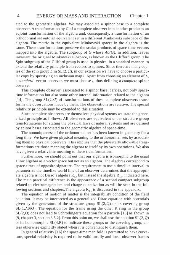
Chapter 1 ENERGY OR MASS AND INTERACTION2
that to obtain the correct motion we must enlarge the chosen group in such a waythat the electromagnetic generators do not commute with the gravitational ones.It is not true that any structure group which contains SL(2,C) U(1) as a sub-group gives a unified theory without contradicting the electrodynamic equationsof motion. The correct classical motion is a fundamental requirement of a unifiedtheory.
In addition to this commutation physical problem there are two mathematicalproblems due to the SO(3,1) group. The second problem is that orthogonal groupsare double valued due to their quadratic metric. The third problem is the definition ofthe square root of unit vectors associated to the metric signature.
Clifford algebras were developed to solve the third problem for general orthonor-mal spaces Rm,n. The geometric elements in the algebras include real numbers R,complex numbers C or R0,1, anticommuting quaternions H or R0,2, Clifford operatorsR3,1 or Cl(3,1)... Cl(m,n), etc. The groups generated by Cl(m,n) solve the threeproblems. They are also useful in taking the square root of operators and have aricher mathematical structure which determines a higher predictive power.
Therefore, we should use the maximal group of Clifford number transforma-tions which preserve the metric and numerical structures of the associated spaces.The construction of the theory was accomplished [7, 8, 9] by taking this group,which is essentially SL(4,), as the structure group G of a generalized curvedelectromagnetic theory. This construction appears to be sufficient to obtain astructure group which describes all known physical energy interactions and cor-responds to Hilbert’s sixth problem [10].
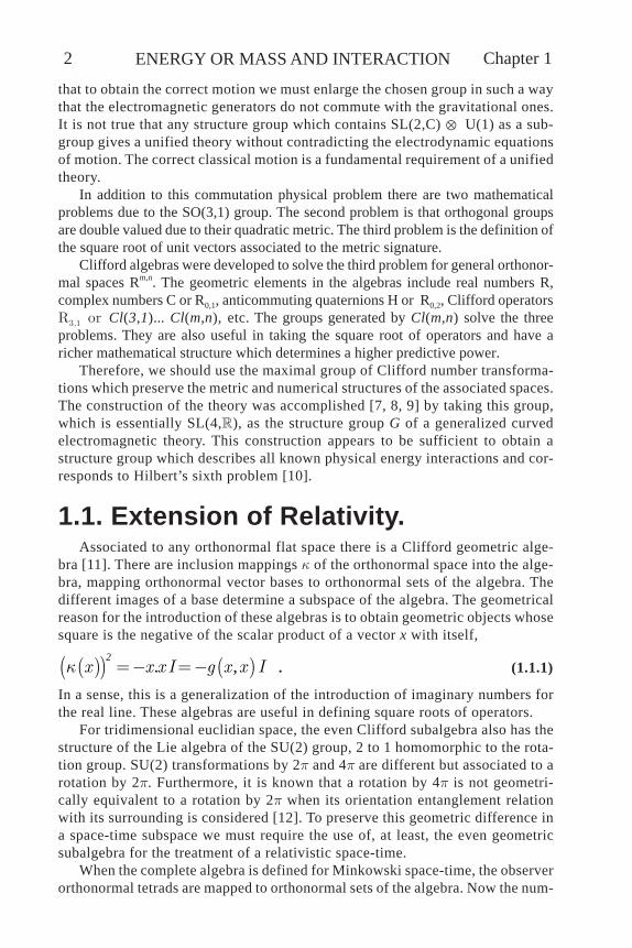
1.1. Extension of Relativity.Associated to any orthonormal flat space there is a Clifford geometric alge-
bra [11]. There are inclusion mappings k of the orthonormal space into the alge-bra, mapping orthonormal vector bases to orthonormal sets of the algebra. Thedifferent images of a base determine a subspace of the algebra. The geometricalreason for the introduction of these algebras is to obtain geometric objects whosesquare is the negative of the scalar product of a vector x with itself,
( )( ) ( ). ,x x x I g x x Ik = - = -2
. (1.1.1)
In a sense, this is a generalization of the introduction of imaginary numbers forthe real line. These algebras are useful in defining square roots of operators.
For tridimensional euclidian space, the even Clifford subalgebra also has thestructure of the Lie algebra of the SU(2) group, 2 to 1 homomorphic to the rota-tion group. SU(2) transformations by 2p and 4p are different but associated to arotation by 2p. Furthermore, it is known that a rotation by 4p is not geometri-cally equivalent to a rotation by 2p when its orientation entanglement relationwith its surrounding is considered [12]. To preserve this geometric difference ina space-time subspace we must require the use of, at least, the even geometricsubalgebra for the treatment of a relativistic space-time.
When the complete algebra is defined for Minkowski space-time, the observerorthonormal tetrads are mapped to orthonormal sets of the algebra. Now the num-

3Energy
ber of possible orthonormal sets in the algebra is much larger than the possibleorthonormal tetrads in space-time. There are operations, within the algebra, whichtransform all possible orthonormal sets among each other. These are the innerautomorphisms of the algebra. Geometrically this means that the algebra spacecontains many copies of the orthonormal Minkowski space. A relativistic ob-server may be imbedded in the algebra in many equivalent ways. It may be saidthat a normal space-time observer is algebraically “blind”. Usually the algebra isrestricted to its even part, when the symmetry is extended from the Lorentz group(automorphisms of space-time) to the corresponding spin group SL(2,C) [13],(automorphisms of the even subalgebra). In this manner a fixed copy of Minkowskispace is chosen within the geometric algebra. This copy remains invariant underthe spin group.
The situation is similar to the imbedding of a three dimensional observer car-rying a spatial triad into tetradimensional space-time. This imbedding is notunique, depending on the relative state of motion of the observer. There are manyspatial tridimensional spaces in space-time, defining the concept of simultaneitywhich is different for observers with different constant velocities. These possiblephysical observers may all be transformed into each other by the group ofautomorphisms of space-time, the Lorentz group.
This similarity allows the extension of the principle of relativity [1] by takingas structure group the group of correlated automorphisms of the space-time geo-metric algebra spinors instead of the group of automorphisms of space-time it-self or only the automorphisms of the even subalgebra spinors. A relativistic ob-server carrying a space-time tetrad is imbedded in the geometric algebra space ina nonunique way, depending on some bias related to the orientation of atetradimensional space-time subspace of the sixteen dimensional algebra. As Diraconce pointed out, we should let the geometrical structure itself lead to its physi-cal meaning.
We may conceive complete observers which are not algebraically “blind”.These observers should be associated to different but equivalent orthonormalsets in the algebra. Transformations among complete observers should producealgebra automorphisms, preserving the algebraic structure. This is the same situ-ation of special relativity for space-time observers and Lorentz transformations.
In particular the inner automorphisms of the algebra are of the form
a a-¢ = 1g g , (1.1.2)where g is an element of the largest subspace contained in the algebra whichconstitutes a group. This action corresponds to the adjoint group acting on thealgebra.
For the Minkowski orthonormal space, denoted by R3,1, the Clifford algebraCl(3,1)=R3,1 is (2), where may be called the ring of pseudoquaternions [9]and the corresponding group is GL(2,). The adjoint of the center of this group,acting on the algebra, corresponds to the identity. The quotient by its normalsubgroup R+ is the simple group SL(2,). Therefore, the simple group nontriviallytransforming the complete observers among each other is SL(2,). This group isprecisely the group G of correlated automorphisms of the spinor space associ-
Chapter 1 ENERGY OR MASS AND INTERACTION4
ated to the geometric algebra. We may associate a spinor base to a completeobserver. A transformation by G of a complete observer into another produces anadjoint transformation of the algebra and, consequently, a transformation of anorthonormal set onto an equivalent set in a different Minkowski subspace of thealgebra. The metric in the equivalent Minkowski spaces in the algebra is thesame. These transformations preserve the scalar products of space-time vectorsmapped into the algebra. The subgroup of G whose Ad(G), in addition, leavesinvariant the original Minkowski subspace, is known as the Clifford group. TheSpin subgroup of the Clifford group is used in physics, in a standard manner, toextend the relativity principle from vectors to spinors. Since there are many cop-ies of the spin group L in SL(2,), in our extension we have to choose a particu-lar copy by specifying an inclusion map i. Apart from choosing an element of L,a standard vector observer, we must choose i, thus defining a complete spinorobserver
This complete observer, associated to a spinor base, carries, not only space-time information but also some other internal information related to the algebra[14]. The group SL(2,) of transformations of these complete observers trans-forms the observations made by them. The observations are relative. The specialrelativity principle may be extended to this situation.
Since complete observers are themselves physical sytems we state the gener-alized principle as follows: All observers are equivalent under structure grouptransformations for stating the physical laws of natural systems and are definedby spinor bases associated to the geometric algebra of space-time.
The nonuniqueness of the orthonormal set has been known in geometry for along time. We have given physical meaning to the orthonormal sets by associat-ing them to physical observers. This implies that the physically allowable trans-formations are those mapping the algebra to itself by its own operations. We alsohave given a relativistic meaning to these transformations.
Furthermore, we should point out that our algebra is isomorphic to the usualDirac algebra as a vector space but not as an algebra. The algebras correspond tospace-times of opposite signature. The requirement to use a timelike interval toparametrize the timelike world line of an observer determines that the appropri-ate algebra is not Dirac´s algebra R1,3 but instead the algebra R3,1, indicated here.The main practical difference is the appearance of a second compact subgrouprelated to electromagnetism and charge quantization as will be seen in the fol-lowing sections and chapters.The algebra R3,1 is discussed in the appendix.
The equation of motion of matter is the integrability condition of the fieldequation. It may be interpreted as a generalized Dirac equation with potentialsgiven by the generators of the structure group SL(2,) or its covering groupSL(1,LQ). The equation for the frame using the other K ring in the groupSL(2,Q) does not lead to Schrödinger’s equation for a particle [15] as shown in[9, chapter 3, section 3.5.2]. From this point on, we shall use the notation SL(2,)or its homomorphic SL(4,R) to indicate these groups or the covering group, un-less otherwise explicitly stated when it is convenient to distinguish them.
In general relativity [16] the space-time manifold is permitted to have curva-ture, special relativity is required to be valid locally and local observer frames
5Energy
are introduced, depending on their positions on space-time. In this manner weget fields of orthonormal tetrads on a curved manifold. The geometry of the mani-fold determines the motion, introducing accelerations of inertial and gravitationalnature.
Similarly in our case, in order to include accelerated systems, we let space-time have curvature and introduce local complete observers which depend ontheir positions. But now, these observers are represented by general spinor frameswhich are subject to transformations beyond relativity (Ultra relativity). In thismanner we get fields of spinor bases (frames) which geometrically are local sec-tions of a fiber bundle with a curved base space. The geometry determines theevolution of matter, but now we have, in addition to inertial and gravitationalaccelerations, other possible accelerations due to other fields of force representedby the additional generators. These algebraic observers are accelerated observ-ers. In other words we now get a geometrically unified theory with extra interac-tions (nuclear and particle) whose properties must be investigated.
1.2. Energy and the Field Equation.The group SL(4,R) is known not to preserve the corresponding metric. But, if
we think of general relativity as linked to general coordinate transformationschanging the form of the metric, it would be in the same spirit to use such agroup. Instead of coordinate transformations whose physical meaning is associ-ated with a change of observers, we have transformations belonging to the struc-ture group whose physical meaning should be associated with a change of spinorsrelated to observers. Representations of this group would be linked to matterfields. If we restrict to the even part of the group, taken as a subset of the Cliffordalgebra, we get the group SL1(2,C), used in spinor physics. Since SL(4,R) islarger (higher dimensional) than SL(2,C) it gives us an opportunity to associatethe extra generators with energy interactions apart from gravitation and electro-magnetism. The generator which plays the role of the electromagnetic generatormust be consistent with its use in other equations of physics. The physical mean-ing of the remaining generators should be identified.
The field equations should relate the interaction connection w or the physi-cally equivalent interaction potential A to a geometric object representing matter.We expect that matter is represented by a current J(m) function of points m on aspace-time manifold M, valued in the group Lie algebra, rather than thenongeometric stress energy tensor T. The simplest object of this type is a gener-alized curvature W of w or the physical generalized Maxwell tensor F. This gen-eralized tensor obeys the Bianchi identity, which we write indicating the covari-ant exterior derivative by D,
DF DWº = 0 . (1.2.1)
The next simple object is constructed using Hodge duality. In similarity withthe linear Maxwell’s theory, we postulate the corresponding nonlinear field equa-tion for the curvature as the generalized geometrical electrodynamic equation,

Chapter 1 ENERGY OR MASS AND INTERACTION6
* *D F D k JW *º = , (1.2.2)where matter is represented by the current *J, which must be a 3-form valued inthe algebra, and k is a constant to be identified later. Because of the geometricalstructure of the theory the source current must be a geometrical object compat-ible with the field equation and the geometry. The structure of J, of course, isgiven in terms of some geometric objects acted upon by the potential. The geo-metrical properties of the curvature and the field equations determine that J obeysan integrability condition,
,DD F F F* *é ù= =ê úë û 0 , (1.2.3)
D J* = 0 . (1.2.4)This relation being an integrability condition on the field equations, includes
all self reaction terms of the matter on itself. A physical system would be repre-sented by matter fields and interaction fields which are solutions to this set ofnonlinear simultaneous equations. There should be no worries about infinitiesproduced by self-reaction terms. As in the EIH method in general relativity [17],when a perturbation is performed on the nonlinear equations, for example toobtain linearity of the equations, the splitting of the equations into equations ofdifferent order brings in the concepts of field produced by the source, force pro-duced by the field and therefore the self-reaction terms. These terms, not presentin the original nonlinear system, are a problem introduced by this particular methodof solution. In the zeroth order a classical particle moves as a test particle with-out self-reaction. In the first order the field produced by the particle produces aself correction to the motion.
Enlarging the group of the potential not only unifies satisfactorily gravitationand electromagnetism [8, 9], but requires other fields [14] and it appears to givea gravitational theory which differs, in principle, from Einstein’s theory and re-sembles Yang’s theory [18]. This may be seen from the field equations of thetheory, which relate the derivatives of the Ehresmann curvature to a current source J.
The product of the interaction potential A by the matter current J has units ofenergy or inverse length. We may naturally define a fundamental unified geometricenergy M associated to the geometry, which defines the concept of mass and ap-pears to be related to the concepts of inertia,
( ) ( ) ( )( )trm J m A mmm= 1
4M . (1.2.5)
This unification of the concept of energy and mass leads to important physicalresults.
A theory of connections without any other objects is incomplete from a geo-metrical point of view. A connection on a principal bundle is related to the struc-ture group and the base space of the bundle. Representations of the group pro-vide a natural vector fiber for an associated vector bundle on which the connec-tion may be made to act. The geometric meaning of the physical potential isrelated to parallel translation of the elements of the fiber at different points

7Energy
throughout the base space. This is, essentially, a process of comparison of ele-ments at different events.
A vector fiber space of this type has a base and the effect of the potential isnaturally defined on the base. From a geometrical point of view the potentialshould be complemented by a vector base. It is well known that Einstein’s gravi-tation theory may be expressed using an orthonormal tetrad instead of the metric[19]. In this theory we have taken this idea one step further, introducing a spinorbase e on the fiber space of an associated vector bundle S, in addition to the baseon the fiber of the tangent space. In other words, we work with the base of the“square root space” of the usual flat space. The potential, which represents thegravitational and electromagnetic fields, depends on a current source term. Wealso postulate that this source current is built from fundamental matter fieldswhich have the geometrical interpretation of forming a base e on the fiber of theassociated vector bundle and defines an orthonormal subset k of the geometricClifford algebra,
!J e edx dx dxm a b g
abgme k* = 13
. (1.2.6)
This base e, when arranged as a matrix with the vectors of the base as col-umns, is related to an element of the group of the principal bundle. It is natural toexpect that a base field e (a section in geometric language), which we shall call aframe e, should obey equations of motion which naturally depend on the poten-tial field. In fact, it will be seen that a particular solution of the integrabilitycondition, the covariant conservation equation (1.2.4) of J, is obtained from theequation
emmk = 0 . (1.2.7)
This equation may be interpreted as a generalized Dirac equation since the struc-ture group is SL(4,R) or its covering group .
We should note that whenever we have an sl(2,C) potential, there is a canoni-cal coupling of standard gravitation to spin ½ particles obtained by postulating aDirac equation which depends on a spin frame [20, 21, 22]. Nevertheless, strictlythis does not represent a real unification. Our field equation implies integrabilityconditions in terms of J. Together with the geometric structure of J, our condi-tions imply the generalized Dirac equation which, therefore, is not required to beseparately postulated, as in the previously mentioned nonunified case. The theoryunder discussion is not a mere pasting together of canonical gravitation and ca-nonical electromagnetism for spin ½ particles. Rather, it is the introduction of ageneralized geometric structure which nontrivially modifies both canonical theo-ries and their coupling. Actually, the nonlinear field equation for the potentialand the simplest geometric structure of the current are sufficient to predict thisgeneralized Dirac equation and provide a unified concept of energy and mass.
If we introduce a variational principle [8,9] to obtain the two fundamentalequations, (1.2.2) and (1.2.4), the principle determines a third related fundamen-tal equation,
Chapter 1 ENERGY OR MASS AND INTERACTION8
()ˆ ˆ ˆˆtr trF F u F F k e u e u e u emmn m kl m n
rn r kl r nri i- -é ùé ù- = - ê ú ê úë û ë û1 14 4 (1.2.8)
which represents the total generalized field energy. It has been shown [8, 9] that thelatter equation leads to the Einstein equation of gravitation in General Relativitywith a geometric tensor source T.
Some of the features of the theory depend only on its geometry and not on aparticular field equation and may be seen directly. For example, matter must evolveas a representation of SL(4,R) instead of the Lorentz group. It follows that matterstates are characterized by three quantum numbers corresponding to the discretenumbers characterizing the states of a representation of SL(4,R). One of thesenumbers is spin, another is associated to the electromagnetic SU(2). This givesus the opportunity to recognize the latter as the electric charge [23].
Perhaps we should realize that the idea of a quantum entered Modern Physicsby the experimental determination of the discreteness of electric charge. Lateratomic measurements were explained by quantum theory by assuming the quan-tum of spin, but quantum theory was not given the burden to quantize electriccharge. The possibility of obtaining the quantum of charge as explained before,may indicate that present day quantum theory is an incomplete theory as Diracindicated [24].
As a bonus, this theory provides a third quantum number for a matter state,which may be recognized as a quantum of magnetic flux, providing a plausiblefundamental explanation to the fractional quantum Hall effect [23].
As in general relativity, the integrability conditions imply the equations ofmotion for a classical particle, without knowledge of the detailed form of thesource J, if we assume that J has a multipole structure. The desired classicalLorentz equations of motion were obtained [1, 7].
Nevertheless the main objective at present, is not to describe the classicalmotion of matter exhaustively but rather to construct the geometrical theory andto show that it is compatible with the classical motion of the sources and withmodern ideas in quantum theory. In particular, it appears, as first objective, toexploit the opportunity provided by the theory to give a geometrical interpreta-tion to the source current in terms of fundamental geometric matter field objects.With the geometric structure given to J, the first stage in the construction of theunified concept of energy is completed.
1.3. Inertial Effects and Mass.The proposed nonlinear equation and its integrability condition have peculiar
aspects which distinguish them from standard equations in classical physics. Nor-mally coupled field equations and equations of motion, for example Maxwelland Lorentz equations, in presence of a current source do not provide, by them-selves, a static internal solution for a source which may represent a particle orobject under the influence of its own field. Use of delta functions for point par-ticles avoid the problem rather than solve it, and may introduce self acceleratedsolutions [25, 26]. The choice of current density in the theory, together with the

9Energy
interpretation developed allows a discussion on different grounds. The frame ethat enters in the current represents matter. Since a measurement is always acomparison between similar objets, a measurement of e entails another frame e’to which its components are referred. If we choose the referential e’ properly wemay find interesting solutions. In particular we can find a geometric backgroundsolution, which we call the substratum, whose excitations behave as particles.
The integrability condition of the nonlinear equation leads to a generalizedDirac equation for the motion of matter, with a parameter that may be identifiedwith a mass defined in terms of energy [7, 8, 9]. The recognition of a singleconcept of mass is fundamental in General Relativity and merits discussion ofpossible solutions of the coupled equations.
If we identify a geometrical excitation with a physical particle, the Dirac equa-tion for a linear excitation, which now would be the linear equation for a particle,contains parameters provided by the curved (nonlinear) background solutionwhich we shall call its substratum solution. Some of the particle properties couldbe determined by a substratum geometry. In particular a mass parameter arisesfor the frame excitation particle from the mass-energy concept defined in termsof energy. It is clear that this parameter is not calculable from the linearizedexcitation equation but rather from a nonlinear substratum solution.This appearsinteresting, but requires a knowledge of a substratum solution to the nonlinearfield equation. Thus it is necessary to find a nonlinear solution, the simpler thebetter, which could illustrate this ideas. It is in this context that the followingsolution is presented.
The nonlinear equations of the theory are applicable to an isolated physicalsystem interacting with itself. Of course the equations must be expressed in termsof components with respect to an arbitrary reference frame. A reference frameadapted to an arbitrary observer introduces arbitrary fields which do not containany information related to the physical system in question. The only nonarbitraryreference frame is the frame defined by the physical system itself.
Any excitation must be associated to a definite background solution or sub-stratum solution. An arbitrary observation of an excitation property depends onboth the excitation and its substratum, but the physical observer must be thesame for both excitation and substratum. We may use the freedom to select thereference frame to refer the excitation to the physical frame defined by its ownsubstratum.
We have chosen the current density 3-form J to beˆ
ˆJ e u em a mak= , (1.3.1)
in terms of the matter spinor frame e and the orthonormal space-time tetrad u .Since we selected that the substratum be referred to itself, the substratum
matter local frame em, referred to er becomes the group identity I. Actually thisgeneralizes comoving coordinates (coordinates adapted to dust matter geode-sics) [27]. We adopt coordinates adapted to local substratum matter frames (theonly nonarbitrary frame is itself, as are the comoving coordinates). If the frame ebecomes the identity I, the comoving substratum current density becomes a con-stant. Comparison of an object with itself gives trivial information. For example

Chapter 1 ENERGY OR MASS AND INTERACTION10
free matter or an observer are always at rest with themselves, no velocity, noacceleration, no self forces, etc. In its own reference frame these effects actuallydisappear. This substratum represents inert matter. Only constant self energy terms,determined by the nonlinearity, make sense and should be the origin of the con-stant bare inertial mass parameter.
At the small distance l, characteristic of excitations, the elements of the sub-stratum, both connection and frame, appear symmetric, independent of space-time. We should remember that space-time M is, mathematically, a locally sym-metric space or hyperbolic manifold [28] . We recognize these as the necessarycondition for the substratum to locally admit a maximal set of Killing vectors[29] which should determine the space-time symmetries of the connection (andcurvature). This means that there are space-time Killing coordinates such thatthe connection is constant but nonzero in the small region of particle interest. Aflat connection does not satisfy the field equation. The excitations may alwaysbe taken around a symmetric nonzero connection or potential.
In particular the nonlinear equation admits a local nonzero constant potentialsolution. This would be the potential determined by an observer at rest with the mat-ter frame. Of course, this solution is trivial but since the potential has units of energy,mass or inverse length, this actually introduces fundamental dimensions in the theory.Furthermore, a constant nonzero solution assigns a constant mass parameter m to afundamental particle excitation and allows the calculation of mass ratios of particlesby integration of M on symmetric spaces [9]. The result is obtained in terms of thedimensionless coupling constant in eq. (1.2.2). Therefore, we wish to find a constantnonzero inert (trivial) solution to the nonlinear field equation which we shall call theinert substratum solution.
First we look into the left side of the field equation (1.2.2), and notice that fora constant potential form A and a flat metric, the expression reduces to triplewedge products of A with itself [9], which may be put in the form of a polyno-mial in the components of A. This cubic polynomial represents a self interactionof the potential field since it may also be considered as a source for thedifferential operator.
Rather than work with the whole group G we first restrict the group to the 10dimensional Sp(4,) subgroup. Furthermore we desire to look at thenongravitational part of the potential. Hence, we limit the components of thepotential to the Minkowski subspace defined by the orthonormal set, which isthe coset Sp(4,)/SL(2,C). This is possible because if the potential is odd so isthe triple product giving an odd current as required. The substratum solution is
ˆˆsA e edx e de J e de e deaapa k L- - - -= - + = - + = +1 1 1 113
43 M . (1.3.2)
where M is a constant determining the equipartition of excitation energy. This inertpotential is essentially proportional to the current, up to an automorphism. It shouldbe noted that in the expression for A, the term containing the current J defines apotential tensorial form L. Its subtraction from A gives an object, e-1de, which trans-forms as a potential or connection. This solution may be extended from the subgroupto the whole 15 dimensional SL(4,R) group using complex coordinates on the com-plex coset SL(4,R)/SL(2,C). We call this solution the complex inert substratum [9].

11Energy
For any potential solution A or connection we can always define a newpotential or connection by subtracting the tensorial potential form L corre-sponding to the substratum solution, eq. (1.3.2),
A A A JLº - = +4
M . (1.3.3)
In terms of the new potential defined by equation (1.3.3) the equation ofmotion (1.2.9), in induced representations, explicitly displays the termdepending on the substratum mass required by the Dirac equation. Using thealgebraic relations among the orthonormal subset k of the geometric Cliffordalgebra we get,
( )
,
e e eA e eA e J
e e e e
m m mm m m m m m
m m mm m m
k k k
k k k k
æ öæ ö÷ç ÷ç = ¶ - = ¶ - + ÷÷ç ç ÷÷çç ÷è øè ø
= + = - =
4
04
M
MM (1.3.4)
which explicitly shows the geometric energy M as the germ of the Dirac particlemass. This equation is nonlinearly coupled to the field equation (1.2.2) through thedefinition of J, eq. (1.2.6).
1.4. The Classical Fields.The curvature of this geometry is a generalized curvature associated to the
group SL(4,R). Since it is known that the even subgroup of SL(4,R) is the Spingroup related to the Lorentz group, we look for a limit theory to get this reduc-tion. When ultra relativistic effects are small, we expect that we can choose basesso that the odd part is small of order e. This is accomplished mathematically bycontracting the SL(4,R) group with respect to its odd subspace [30]. In the con-tracted group this odd subspace becomes an abelian subspace. Then the SL(4,R)curvature reduces to
( )F F e+= +O , (1.4.1)
where F + is the curvature of the even subgroup SL1(2,C)The result is that in this limit the curvature reduces to its even component
which splits into an SL(2,C) curvature and a separate commuting U(1) curvature.It is known that an SL(2,C) curvature may represent gravitation [31] and a U(1)curvature may represent electromagnetism [32, 33, 34].
If we take this limit U(1) as representing the standard physical electromagne-tism we must accept that, in the full theory, electromagnetism is related to theSU(2) subgroup of SL(4,R) obtained using the inner automorphisms. Similarlythe SL(2,C) of gravitation may be transformed into an equivalent subgroup by anautomorphism. This ambiguity of the subgroups within G represents a symmetryof the interactions. Since the noncompact generators are equivalent to space-
Chapter 1 ENERGY OR MASS AND INTERACTION12
time boosts, their generated symmetry may be considered external. The internalsymmetry is determined by the compact nonrotational SU(2) sector.
It is well known in special relativity, that motion produces a relativity of elec-tric and magnetic fields. We find, since SL(4,R) acts on the curvature, an intrin-sic relativity of the unified fields, altering the nonunified fields which are seenby an observer. Given the orthonormal set corresponding to an observer, theSL(4,R) curvature may be decomposed in terms of a base generated by the set.The quadratic terms correspond to the SL(2,C) curvature and its associated Ri-emann curvature seen by the observer. A field named gravitation by an observer,may appear different to another observer. These transformations disguise inter-actions into each other.
The algebra associates some generators to space-time and simultaneously tosome interactions. This appears surprising, but on a closer look this is a naturalassociation. In an experiment, changes due to an interaction generator are inter-preted by an observer as time and distance which become parameters of change.Then, it is natural that a reorientation, a gyre of space-time within the algebracorresponds to a rearrangement of interactions. A complete observer has thecapacity to sense forces not imputable to his space-time riemannian curvature.He senses them as nongravitational, nonriemannian, forces. This capacity maybe interpreted as the capacity to carry some generalized charge corresponding tothe nongravitational interactions. Ultra relativity is essentially interpreted as anintrinsic relativity of energy interactions.
We should separate the equations with respect to the even subalgebra or sub-group as indicated by eq. (1.4.1), because this part represents the classical fields.In other words, we have the sl1(2,C) forms, as functions of its generators i, E,
aaA A I Ei G+ = + , (1.4.2)
n n aaF F I R Ei+ = + . (1.4.3)
It should be noted that the even curvature does not just arise from the even partof the connection because it depends on the product of odd parts.
The curvature F of the abelian even connection A corresponds to the Maxwellcurvature tensor in electrodynamics and obeys
* *D F d F k j jpa* *= = º 4 , (1.4.4)
DF dF= = 0 , (1.4.5)which are exactly the standard Maxwell’s equations if we define k in terms of thefine structure constant a. The standard j.A interaction is obtained back.
The curvature form R of the G connection corresponds to the Riemann curva-ture with torsion, in standard spinor formulation. They obey the equations
*D R k J* += , (1.4.6)
DR = 0 , (1.4.7)

13Energy
which are not Einstein’s equations but represent a spinor gravitation formulationequivalent to Yang’s [18] theory restricted to its SO(3,1) subgroup.
It may be claimed that the Einstein equation of the geometric unified theoryis equation (1.2.8) rather than the field equation. In general this equation may bewritten in terms of the Einstein tensor G [8, 9]
( )j g t cn
GRrm rm rm rm rmp Q p Q Q Qé ù= - + +ê úë û3 8 8 . (1.4.8)
We have then a generalized Einstein equation with geometric stress energytensors.
When we consider the external field problem, that is, space-time regionswhere there is no matter, the gravitational part of the field equations for J=0are similar to those of Yang’s gravitational theory. All vacuum solutions ofEinstein’s equation are solutions of these equations. In particular theSchwarzchild metric is a solution and, therefore, the newtonian motion under a1/r gravitational potential is obtained as a limit of the geodesic motion underthe proposed equations.
Nevertheless, in the interior field problem there are differences between theunified physical geometry and Einstein’s theory. For this problem where thesource J is nonzero, our theory is also essentially different from Yang’s theory.Since in the physical geometry the metric and the so(3,1) potential remaincompatible, the base space remains pseudoriemannian with torsion avoidingthe difficulties discussed by Fairchild and others for Yang’s theory. Thisequation may be interpreted as the existence of an apparent effective stress en-ergy tensor which includes contributions from “dark matter or dark energy”.
1.5. Results.The physical universe is described by matter equations associated to an evo-
lution group. The group is obtained from geometric algebraic tranformations ofrelativistic space and time. The related algebra is essentially the Pauli matricesmultiplied by the quaternions, as indicated in the appendix. The interaction isrepresented by field equations and equations of motion in terms of potential andforce tensors determined by matter transformation currents. We identify the con-cept of energy using the potential and current fields.
A nonlinear particular solution, which may represent inertial properties, wasgiven. The concept of bare inertial mass is related to this solution. Microscopicphysics is seen as the study of linear geometric excitations.
The results obtained indicate that gravitation and electromagnetism are uni-fied in a nontrivial manner. There are additional generators which may representnon classical nuclear and particle interactions [9]. Strong nuclear electromagne-tism is related to an SU(2)Q subgroup. If we exclusively restrict to a U(1) sub-group we obtain Maxwell’s field equations. We have a generalized Einstein equa-tion with geometric stress energy tensors and possible dark matter effects.
2. Quanta.The geometrical structure of the theory, in terms of a potential describing the
interaction and a frame describing matter, is determined by the field equationswhich relate the generalized curvature to the matter distribution. Neverthelesssome aspects of the theory may be discussed by group techniques without neces-sarily solving the field equations.
The structure group of the theory, SL(2,), the group of spinor automorphismsof the universal Clifford algebra of the tangent space at a space-time point, actson associated spinor bundles and has generators which may represent other in-teractions, apart from gravitation and electromagnetism. A consequence of thetheory is the necessary association of electromagnetism to an SU(2) subgroup ofSL(2,).
In order to give a complete picture, the frame fields should represent matterand, consequently, the frame excitations should represent particles. The poten-tial acts on the frame excitations which may be considered linear representationsof the group. It is of interest to consider the irreducible representations of thisgroup and to discuss its physical interpretation and predictions [8]. Representa-tions of related groups have been discussed previously [35 ].
2.1. Induced Representations of theStructure Group G.
The irreducible representations of a group G may be induced from those of asubgroup H. These representations act on the sections [36 ] of a homogeneousvector bundle over the coset space M = G/H with fiber the carrier space U of therepresentations of H.
It is then convenient to consider the subgroups contained in SL(2,), in par-ticular the maximal compact subgroup. The higher dimensional simple subgroupsare as follows:
1. The 10-dimensional group P, generated by ka, k[akb]. This group is iso-morphic to subgroups generated by k[akbkg], k[akb] and by k[akbkc], k[akb],k5;
2. The 6-dimensional group L, corresponding to the even generators ofthe algebra, k[akb]. This group is isomorphic to the subgroups gener-ated by ka, k[akb] and by k0k[akb], k[akb];
3. There are two compact subgroups, generated by k[akb] and by k0, k5,k1k2k3.
The P subgroup is, in fact, Sp(2,), homomorphic to Sp(4,), as may beverified by explicitly showing that the generators satisfy the simplectic require-ments [37 ]. This group is known to be homomorphic to SO(3,2), a De Sittergroup. The L subgroup is isomorphic to SL(2,). The compact subgroups areboth isomorphic to SU(2) and therefore the maximal compact subgroup of the

15Quanta
covering group G is SU(2)ÄSU(2) homomorphic to SO(4). The LPG chaininternal symmetry is SU(2)U(1) and coincides with the symmetry of the weakinteractions.
Irreducible representations of the covering group of SL(2,) may be inducedfrom its maximal compact subgroup. The representations are characterized bythe quantum numbers associated to irreducible representations of both SU(2)subgroups. These representations may be considered sections of an homogeneous
vector bundle over the coset SL(4, ) /(SU(2)ÄSU(2)) with fiber the carrier spaceof representations of SU(2)ÄSU(2).
One of the SU(2), acting on spinor space, is associated to the rotation group,acting on vector space. Its irreducible representations are characterized by a quan-tum number l of the associated Casimir operator L2, representing total angularmomentum squared. The other SU(2), as indicated in previous sections, may beassociated to electromagnetism. It has a Casimir operator C2, similar to L2 butrepresenting generalized total charge, with some quantum number c. The irre-ducible representations of SL(2,) have a third label which may be associated toone of the Casimir operators of SL(2,), for example, the quadratic operator M2
on the symmetric space SL(4,)/SO(4).The states of these irreducible representations of SL(2,) should be charac-
terized by integers m, q corresponding to physical particles with z component ofangular momentum m/2 and charge qe. These quantum numbers are studied indetail in chapters 2 and 3. The price paid to obtain this charge quantization isonly the association of electromagnetism to the second SU(2) in SL(2,). Infact, this may not be a disadvantage in a unified theory of this type, where it maylead to new geometric representations of physical phenomena. It should be notedthat Dirac’s charge quantization scheme [38 ] requires the existence of magneticmonopoles. This requirement is not compatible with this theory.
Representations of SL(2,) may also be induced from L, naturally including thespin representations of its SU(2) subgroup. Since L is a subgroup of P, it is moreinteresting to look at the representations induced from P which include, in particular,those of L. In some situations the holonomy group of the potential or connection maybe P= Sp(2,) and we may expect that representations induced from it should playan interesting role. It should be clear that the coset P/L is the De Sitter space S- [39 ].The points of S- may be seen as translation operators on the space S- itself, in thesame manner as the Minkowski space. The Laplace-Beltrami operators on S- haveeigenvalues that should correspond to the concept of mass in this curved space. Theisotropy subgroup at a translation (point) in S- is the rotation subgroup SO(3) fortranslations along lines inside the null 3-hypercone and the SO(2,1) subgroup fortranslations along the lines in the null 3-hypercone itself. The SL(2,) representa-tions induced from the De Sitter group P are characterized by mass and spin or helicityand expressed as sections (functions) of a bundle over the mass shell 3-hyperboloidor the null 3-hypercone, respectively for massive or null mass representations as thecase may be. These representations are solutions of Dirac’s equation in this curvedspace and geometrically correspond to sections of bundles over subspaces of the DeSitter space S-.

Chapter 2 ENERGY OR MASS AND INTERACTION16
The group SO(3,2), homomorphic to Sp(2,), is known [37] to contract toISO(3,1) which is the Poincare group and we may have approximate representa-tions of SL(2,) related to the Poincare group. Then, the representations of thedirect product of Wigner’s little group [40 ] by the translations are introducedapproximately in the theory. The SO(2,1) isotropy subgroup of P contracts to theISO(2) subgroup of ISO(3,1).Thus, we may work with representations character-ized by mass and spin or helicity expressed as sections (functions) of a bundleover the mass shell 3-hyperboloid or the light cone, as the case may be. It shouldbe clear from these considerations of groups that the standard Dirac equation,which is an equation for a representation of the Poincare group, plays an ap-proximate role in the geometric theory.
We should point out that the isotropy subgroup of P at a De Sitter translation(point) in a null subspace is the group of transformations which leaves invariantthe null tangent vectors at the given translation. The isotropy subgroup is SO(2,1)acting on the curved De Sitter translations space or its contraction ISO(2) actingon the flat Minkowski translations space. In either case there is only one rotationgenerator, which corresponds to the common compact SO(2) subgroup in bothisotropy subgroups. Therefore, the null mass representations induced from P arecharacterized by the corresponding eigenvalue or SO(2) quantum number whichis known as helicity. For the rest of the chapter we shall restrict ourselves tomassive representations.
In order to study the irreducible representations of the group SL(2,), weneed to introduce the complex extension of this group, which is SL(4,). Therelation of induced representations with those obtained in Cartan’s approach [41],is discussed in [9]. The Cartan subspace of the complex algebra sl(4,), alsoknown as the root space A3, describes the commutation relations of the canonicalCartan generators of this complex algebra and all its real forms sl(4,), su(4),su(3,1), su(2,2) and su*(4) [9] . In particular, the real form sl(4,) is the leastcompact real form of sl(4,).
2.2. Relation Among QuantumNumbers.
The relation of the quantum numbers associated to the standard Cartangenerators Gi with the quantum numbers of the representations induced from themaximal compact subgroup may be seen by considering the corresponding Cartansubalgebras. There are other Cartan subalgebras in sl(4,). It is known that aCartan subalgebra is not uniquely determined but depends on the choice of aregular element in the complete algebra. Nevertheless, it is also known that thereis an automorphism of the complex algebra which maps any two Cartansubalgebras [41]. This implies there is a relation between the sets of quantumnumbers associated to two different Cartan subalgebras within sl(4,). We maytake the quantum numbers linked to spin and charge as the physically fundamentalquantum numbers and consider the others which arise by use of different Cartansubalgebras as numbers which are functions of the fundamental ones.

17Quanta
For physical reasons, since electromagnetism and electric charge are associatedto the SU(2) subgroup generated by k0, k1k2k3, k0k1k2k3 within our geometrictheory, it is of interest to consider an algebra decomposition with respect to oneof these generators giving a new set of generatos X. Since all three of themcommute with all the generators of the spin SU(2), k1k2, k2k3, and k3k1, we havedifferent choices at our disposal. For convenience of interpretation we choosek1k2, and k0k1k2k3 as our starting point. The only other generator which commuteswith them is k0k3. It has been shown [9] now that neither k0k1k2k3 nor k1k2 areregular elements of the total sl(4,) algebra in spite of being regular elements ofthe two su(2) subalgebras. Each of the two matrices, k1k2 and k0k1k2k3, generatesa subspace Vo, corresponding to eigenvalues l=0, which is seven-dimensional.Since the Cartan subalgebra of sl(4,) is tridimensional, it follows that neither ofthe two generators is a regular element. Nevertheless the sum generator,
( )ad k k k k k k+1 2 0 1 2 3 has a VO subspace, for l=0, which is tridimensional.Therefore, the sum generator is a regular element of the Lie algebra.
The VO space generated by this regular element is a Cartan subalgebra whichis spanned by the generators
X k k=1 1 2 , (2.2.1)
X k k k k=2 0 1 2 3 , (2.2.2)
X k k=3 0 3 , (2.2.3)
where the product is understood in the enveloping Clifford algebra.It is clear that X1, and X2 are compact generators and therefore have imaginary
eigenvalues. Because of the way they were constructed, they should be associated,respectively, to z-component of angular momentum and electric charge. Both ofthem may be diagonalized simultaneously in terms of their imaginary eigenvalues,leaving X3 invariant. When dealing with compact elements of a real form, asspin, it is usual to introduce the standard notation in terms of the correspondingnoncompact real matrices of the real base in the complex algebra.
The Clifford algebra matrices provide a geometric normalization of roots andweights in the Cartan subspace. The weight vectors in the base Xi have the samestructure of those in Cartan’s canonical base except for a standard normalizationfactor of (32)-1/2. Similarly, the roots in both bases have the same structure,differing by the standard normalization factor.
2.3. Spin, Charge and Flux.It may be seen that, in the fundamental representation, one of the generators
in the Cartan subalgebra may be expressed as a Clifford product (not a Lie product)of the other generators of the subalgebra,
X X X=1 2 3 . (2.3.1)

Chapter 2 ENERGY OR MASS AND INTERACTION18
This implies that, within the Clifford algebra, there is a multiplicative relationamong the quantum numbers in the theory. In particular, the z-component angularmomentum generator, spin, is the Clifford product of the electric charge generatorand the X3 generator. The quantum numbers associated to X3 must have the physicalmeaning of angular momentum divided by electric charge, or equivalently,magnetic flux. Then the fundamental quantum of action should be the product ofthe fundamental quantum of charge times the fundamental quantum of flux,
( )h he e=2 2 . (2.3.2)
We may intuitively interpret the last equation as a quantum betatron effect, whena quantum change in magnetic flux is related to a quantum change in angularmomentum.
We have taken the quantum of action in terms of h rather than because thenatural unit of frequency is cycles per second. Then the quantum of flux f0 is
he e
pf = =0 2 . (2.3.3)
The four members of the fundamental irreducible representation form atetrahedron in the tridimensional A3 Cartan space as shown in figure 1. Theyrepresent the combination of the two spin states and the two charge states of anassociated particle, which we shall call a G-particle. One charge state representsa physical particle state and the other represents a charge conjugate state. The G-particle carries one quantum each of angular momentum, electric charge andmagnetic flux and may be in one of the four state whose quantum numbers are:
spin charge flux negative charge with spin up
negative charge with spin down positive charge with spin up
positive charge with spin down
f
f
f
f
-
-
+
+
+ - -- - ++ ++
-- +
1 1 11 1 11 11
11 1
The dual of the fundamental representation, defined by antisymmetric tensorproducts of 3 states of the fundamental representation or triads, corresponds tothe inverted tetrahedron. A conjugate state or a dual state may be related to anantiparticle. This may be useful but is not a necessary interpretation. It is betterto keep these mathematical concepts physically separate. We consider, on onehand, fundamental excitations and dual excitations and, on the other hand,excitations with particle and conjugate states.
The states of an irreducible representation of higher dimensions, built fromthe fundamental one, are also characterized by three integers: angular momentumm, electric charge q and magnetic flux f. We may conjecture then that the magneticmoment is not as fundamental as the magnetic flux when describing particles.

19Quanta
(-1, -1, 1)
(-1, 1, -1)
(1, 1, 1)
(1, -1, -1)
k k k k0 1 2 3 charge
k k0 3 flux
k k1 2 spin
Figure 1.Irreducible representation
of SL(4,R).
2.4. Representations of a Subgroup P.It is known that the SL(2,) subgroup has a unidimensional Cartan subspace
of type A1 associated to the quantized values of angular momentum. The Sp(4,)subgroup has a bidimensional Cartan subspace of type C2. In the same way wehandled SL(4,), we may choose a regular element associated to the spin and
flux generators in particular ( )ad k k k k+1 2 0 3 , which annihilates the bidimensionalsubspace, with zero eigenvalues, spanned by the k1k2 and k0k3 generators. Wemay obtain the corresponding weight vectors and roots with the same previousnormalization. Nevertheless we may also choose as regular element another
element related to the charge in particular, ( )ad k k k+1 2 0 which annihilates thebidimensional subspace, with zero eigenvalues, spanned by the generators k1k2and k0.
In both cases the four members of the fundamental representation form a squarein a bidimensional C2 Cartan space, but in different Cartan subspaces of the A3
root space. We may visualize the relation of these vectors with those of the fullSL(4,) group recognizing that the tridimensional Cartan A3 space collapses to abidimensional C2 subspace as indicated in figure 1. The tetrahedron whichrepresents the states of the fundamental representation collapses to a square. The4 tetrahedron vertices project to the 4 square vertices. The set of 4 weight vectorsin C2 may be obtained by projecting the 4 weight vectors in A3, which correspondto the tetrahedron vertices, on the plane spanned by the vectors k1k2 y k0k3 or
Chapter 2 ENERGY OR MASS AND INTERACTION20
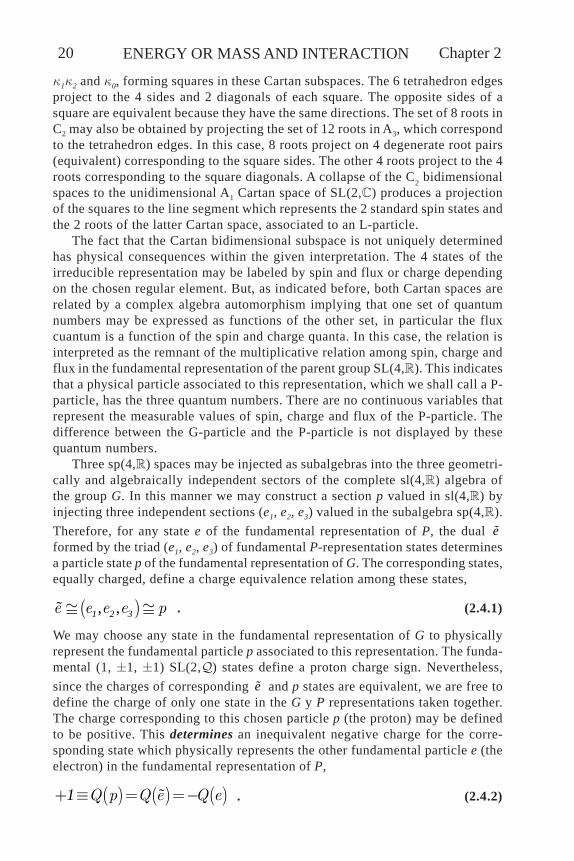
k1k2 and k0, forming squares in these Cartan subspaces. The 6 tetrahedron edgesproject to the 4 sides and 2 diagonals of each square. The opposite sides of asquare are equivalent because they have the same directions. The set of 8 roots inC2 may also be obtained by projecting the set of 12 roots in A3, which correspondto the tetrahedron edges. In this case, 8 roots project on 4 degenerate root pairs(equivalent) corresponding to the square sides. The other 4 roots project to the 4roots corresponding to the square diagonals. A collapse of the C2 bidimensionalspaces to the unidimensional A1 Cartan space of SL(2,) produces a projectionof the squares to the line segment which represents the 2 standard spin states andthe 2 roots of the latter Cartan space, associated to an L-particle.
The fact that the Cartan bidimensional subspace is not uniquely determinedhas physical consequences within the given interpretation. The 4 states of theirreducible representation may be labeled by spin and flux or charge dependingon the chosen regular element. But, as indicated before, both Cartan spaces arerelated by a complex algebra automorphism implying that one set of quantumnumbers may be expressed as functions of the other set, in particular the fluxcuantum is a function of the spin and charge quanta. In this case, the relation isinterpreted as the remnant of the multiplicative relation among spin, charge andflux in the fundamental representation of the parent group SL(4,). This indicatesthat a physical particle associated to this representation, which we shall call a P-particle, has the three quantum numbers. There are no continuous variables thatrepresent the measurable values of spin, charge and flux of the P-particle. Thedifference between the G-particle and the P-particle is not displayed by thesequantum numbers.
Three sp(4,) spaces may be injected as subalgebras into the three geometri-cally and algebraically independent sectors of the complete sl(4,) algebra ofthe group G. In this manner we may construct a section p valued in sl(4,) byinjecting three independent sections (e1, e2, e3) valued in the subalgebra sp(4,).Therefore, for any state e of the fundamental representation of P, the dual eformed by the triad (e1, e2, e3) of fundamental P-representation states determinesa particle state p of the fundamental representation of G. The corresponding states,equally charged, define a charge equivalence relation among these states,
( ), ,e e e e p@ @1 2 3 . (2.4.1)
We may choose any state in the fundamental representation of G to physicallyrepresent the fundamental particle p associated to this representation. The funda-mental (1, 1, 1) SL(2,) states define a proton charge sign. Nevertheless,since the charges of corresponding e and p states are equivalent, we are free todefine the charge of only one state in the G y P representations taken together.The charge corresponding to this chosen particle p (the proton) may be definedto be positive. This determines an inequivalent negative charge for the corre-sponding state which physically represents the other fundamental particle e (theelectron) in the fundamental representation of P,
( ) ( ) ( )Q p Q e Q e+ º = =-1 . (2.4.2)
21Quanta
In other words the charge of the electron (dual) particle must have a sign oppo-site to the charge sign of the proton (dual) particle.
2.5. Magnetic Flux Quanta.From the previous discussion it follows that any particle which is a fundamental
representation of SL(4,) or Sp(4,) must be a charged particle with a quantumof flux. This quantum of flux is exactly the value determined experimentally byDeaver and Fairbank [42 ] and Doll and Nebauer [43 ], first predicted theoreticallyby London [44 ] with an extra factor of two. The experiment consisted in makinga small cylinder of superconductor by electroplating a thin layer of tin on a copperwire. The wire was put in a magnetic field, and the temperature reduced until thetin became a superconducting ring. Afterwards the external field was eliminated,leaving a trapped minimum of flux through the ring.
Our result is consistent with the experimental result if we consider that thetrapped flux through the cylindrical ring layer of superconducting tin is reallyassociated to the discrete minimum intrinsic flux of a single electron inside thenormal (not superconducting) copper wire which serves as nucleus for thesuperconducting tin. At present, it is generally believed that the quantization offlux is due to the topology of the superconducting material in the experiment andrelated to the charge of an electron pair inside the superconductor. The ideaexpressed here is that the quantum of flux is an intrinsic property of matter particles(electron, proton etc.) and only the possibility of trapping the flux depends onthe topology of the superconductor.
The generalization of the Lorentz group (automorphisms of Minkowski space)to the group of automorphisms of the geometric algebra of Minkowski space andthe corresponding physical interpretation indicate that any massive particle (orquasi particle) must carry not only quanta of angular momentum, but also quantaof charge e and quanta of magnetic flux, h/2e , (one or more), both intrinsic andorbital,
( )hNf eF = 2 . (2.5.1)
This equation provides a simple-minded interpretation for the Meissner effect[45] on superconductors. This expression should still be valid if the electrons arepaired. If the pairing is such that the quanta of flux cancel each other, the valueof f should be zero for each pair and consequently the total magnetic flux insidethe superconductor should also be zero.
Furthermore, if a particle crosses a line in a plane normal to its flux, there isa relation between the charge and flux crossing the line. If there are no resistivelosses on a conductor along the line, the induced voltage leads to a transverseresistance which is fractionally quantized,
( )hf eQ qe
DFD
= 2 . (2.5.2)
Chapter 2 ENERGY OR MASS AND INTERACTION22
This expression leads us to conjecture that the fractional quantized Hall effect(FQHE) [46, 47] gives evidence for the existence of these flux quanta instead ofevidence for the existence of fractional charges. The FQHE experiment consistsessentially of the measurement of the transverse Hall conductivity occurring atlow temperature in bidimensional electron gas crystal interfaces insemiconductors.
2.6. Magnetic Energy Levels.Usually the motion in a constant magnetic field is discussed in cartesian coor-
dinates in terms of states with definite energy and a definite linear momentumcomponent. The resultant Landau energy levels are degenerate in terms of themomentum component. Additionally, for the electron, the Landau energy levelsare doubly degenerate except the lowest level. In order to use definite angularmomentum states, the problem is expressed in cylindrical coordinates and theenergy of the levels is [48, 49],
( )eBU n m sMc
= + + +12
, (2.6.1)
where B is the magnetic field along the positive z symmetry axis, m is the abso-lute value of the orbital angular momentum quantum number, also along the posi-tive z axis, n is a nonnegative quantum number associated to the radial wavefunction and s is the spin. This expression has the peculiarity that even for zero mthere may be energy quanta associated to the radial direction.
The equations of motion of charged particles in a constant magnetic field, inquantum or classical mechanics, do not determine the momentum or the center ofrotation of the particle. These variables are the result of a previous process thatprepares the state of the particle. We can idealize this process as a collision be-tween the particle and the field. Since the magnetic field does not do work on theparticle, the energy of the particle is conserved if the system remains isolatedafter the initial collision. The angular momentum of the particle with respect tothe eventual center of motion is also conserved. The values of angular momen-tum and energy inside the field equal their values outside. This implies there isno kinetic energy associated to the radial wave function, as the equation allows.Therefore, among the possible values of energy we must exclude all values of nexcept the value zero. This means that the energy only depends on angular mo-mentum, as in the classical theory.
The degeneracy of energy levels, apart from that due to the momentum compo-nent along the field, is the one due to the spin direction, as in the case of cartesiancoordinates. Only moving electrons make a contribution to the Hall effect, hence wedisregard zero orbital angular momentum states. Each degenerate energy level hastwo electrons, one with spin down and orbital momentum m+1 and the other withspin up and orbital angular momentum m. Each typical degenerate energy level maybe considered to have a total charge q equal to 2e, total spin 0 and a total integerorbital angular momentum 2m+1. Using half integer units,

23Quanta
( )( )zL m= +2 2 1 2 . (2.6.2 )
In the classical treatment of motion in a magnetic field, it is known that theclassical kinetic momentum of a particle has a circulation around the closed curvecorresponding to a given orbit, which is twice the circulation of the canonicalmomentum. The latter, in turn, equals the negative of the external magnetic fluxenclosed by the loop [50 ]. That is, for the given number of quanta of orbitalangular momentum in a typical level, we should associate a number of orbitalexternal magnetic flux quanta. In accordance with the previous equation, we as-sign a flux FL to a degenerate level,
( )( )Lhm eF = - +2 2 1 2 . (2.6.3)
When we have an electron gas instead of a single electron, the electrons occupya number of the available states in the energy levels depending on the Fermi level.The orbiting electrons are effective circular currents which induce a magnetic fluxantiparallel to the external flux. The electron gas behaves as a diamagnetic body,where the applied field is reduced to a net field because of the induced field of theelectronic motion. Associated to the macroscopic magnetization M, magnetic induc-tion B and magnetic field H we introduce, respectively, a quantum magnetizationflux FM, a quantum net B flux FB and a quantum bare H flux FH per level, whichmust be related by
B H MF F F= + . (2.6.4 )
The first energy level of moving electrons is nondegenerate, correspondingto one electron with spin down and one quantum of orbital momentum. In orderfor the electron to orbit, there has to be a net (orbital) flux inside the orbit. If theflux is quantized, the minimum possible is one quantum of orbital flux for theelectron. In addition, another quantum is required by the intrinsic flux asociatedto the intrinsic spin of the electron. Therefore without further equations, the mini-mum number of net quanta in this level is 2 and its minimum net magnetic flux is
( )B
he
F = 22
. (2.6.5)
It should be noted that the minimum flux attached to the electron, in this state, istwice the flux quantum. In other words, the attached flux is split into orbital andintrinsic parts.
The quantum magnetization flux is, considering its induced flux FL opposedto FH , two negatve (-2) quanta for the orbital motion of the single electron andone (1) additional quantum for its intrinsic flux FS, which gives, for thisnondegenerate level, a relation indicating an equivalent magnetic permeabilityof 2/3,
B MF F= 2 . (2.6.7)
Chapter 2 ENERGY OR MASS AND INTERACTION24
This reasoning is not applicable to the calculation of FB for the degeneratelevels in the electron gas, rather, we somehow have to find a relation with FH . Todetermine this exactly we would need to solve the (quantum) equation of motionfor the electrons simultaneously with the (quantum) electromagnetic equationdetermining the field produced by the circulating electrons. Instead of detailedequations we recognize that, since flux is quantized, the orbital flux must changeby discrete quanta as the higher energy levels become active. As the angularmomenta of the levels increase, a proportional increase in any two of the vari-ables in equation (2.6.4 ) would mean that the magnetic permeability does notvary from the value 2/3 determined by the nondegenerate level. Therefore, ingeneral, the flux increases should obey the following quantum condition: theflux FB may deviate discretely from the proportionality indicated by the lastrelation, by an integral number of flux quanta according to,
B MF F DF= +2 , (2.6.8)
where DF is an indeterminate quantum flux of the electron pair in the degeneratelevel. The magnetization flux FM has FL an upper bound and we may indicatethe attached quanta by the inequality
( ) ( )Bh hm e eF dé ù£ + +ê úë û
2 2 2 1 2 , (2.6.9)
where d is an integer indicating a jump in the flux associated to each electron in the pair.Whatever flux FB results, it must be a function of only the flux quanta per elec-
tron pair. A degenerate energy level consists of the combination or coupling of twoelectrons with orbital momentum levels m and m+1, in states of opposite spins, with2m orbital flux quanta linked to the first electron and 2m+2 linked to the other elec-tron. The pair, has 2(2m+1) flux quanta, in terms of a nonnegative integer m. Hencethe only independent variable determining the jump in the flux FB is 2(2m+1). Inorder for FB to be only a function of this variable, the integer d must be even so thatit adds to m, giving the possible values of the net flux of the level,
( )( )Bh
eF m= +4 2 1 2 , (2.6.10)
The physical interpretation of the last equation is the following: If the externalmagnetic field increases, both the effective net magnetic flux B and the effec-tive magnetization flux M per electron increase discretely, by quantum jumps,and the equivalent permeability remains constant.
The number of possible quanta, indicated by f, linked to this level called asuperfluxed level, is
( )f m= +4 2 1 , (2.6.11)
where the flux index m has undetermined upper bound. The number of electriccharge quanta per level, indicated by q, is
q = 2 . (2.6.12)

25Quanta
2.7. Fractional Quantum Hall Effects.Each single electronic state is degenerate with a finite multiplicity. This gives
the population of each typical energy half-level corresponding to a single elec-tron, indicated by N0, when it is exactly full. It is clear that if the degeneracy inthe energy levels is lifted, by the mechanism described in the references, halflevels may be filled separately and observed experimentally.
Since there is the same number of electrons N0 in each sublevel we mayassociate one electron from each sublevel to a definite center of rotation, as amagnetic vortex. We have then, as a typical carrier model, a system of electronsrotating around a magnetic center, like a flat magnetic atom (quasi particle?).The validity of this vortex model relies in the possibility that the levels remainsome how chained together, otherwise, the levels would move independently ofeach other. A physical chaining mechanism is clear: If we have two current loopslinked by a common flux, and one loop moves reducing the flux through theother, Lenz’s law would produce a reaction which opposes the motion of the firstloop, trying to keep the loops chained together.
The total electronic population when the levels are exactly full is,
( ) oqN N N Nn n= + = +0 02 2 1 , (2.7.1)
where n doubly degenerate Landau energy levels are full and where the first N0corresponds to the nondegenerate first Landau level. The charge index n is aninteger if the highest full level is a complete level, or a half integer if the highestfull level is a half level or zero if the only full level is the nondegenerate firstlevel.
The flux linked to this vortex, whatever quantum theory wave functions char-acterize the states of the electronic matter, should have quanta because the sys-tem is a representation that must carry definite quanta of charge, angular mo-mentum and magnetic flux. In other words, the vortex carries quanta of magneticflux. The flux linking a particular vortex is equal to the net flux FB chained bythe orbit of the electron pair corresponding to the highest level. The value of f,the number of net quanta linked to a vortex, is expressed by equation (2.6.11)depending on value of the flux index m for the highest level in the system.
We now make the assumption that the condition for filling the Landau levelsshould be taken in the sense given previously [9, 48] by counting the net fluxquanta linked to the orbital motion of all N0 vortices. The filling condition isdetermined by conservation of flux (continuity of flux lines). The applied exter-nal flux must equal the total net flux linked only to the highest level. This deter-mines a partial filling of the levels, in the canonical sense (only h/e per electron).This filling condition implies, for a degenerate level with N0 pairs,
hf
N eF æ ö÷ç= ÷ç ÷çè ø0 2
. (2.7.2)
The general expression for the Hall conductivity, in terms of the bidimensionaldensity of carriers N/A and the number of quanta of the carriers q, is

Chapter 2 ENERGY OR MASS AND INTERACTION26
qeNAB
s = . (2.7.3)
Substituting, we obtain for the conductivity, for values of q an f given by equa-tions (2.6.11), (2.6.12),
( )( )
, e N e
h
n ns n
F m
æ ö+ + ÷ç ÷= = ³ç ÷ç ÷ç+ è ø
20 1
2
2 1 2 12 2 1
. (2.7.4)
This expression is not valid if the highest level is the nondegenerate firstlevel. For this special case, where n is equal to zero, there are separate values forq and f ,
hf
N eF æ ö÷ç= ÷ç ÷çè ø0
0 2 , (2.7.5)
and, we get, using equation (2.6.5),
, eN e ef h h
s nF
æ ö÷ç ÷= = = =ç ÷ç ÷çè ø
2 20
0
1 2 0 . (2.7.6)
For half integer n we may define another half integer n which indicates thenumber of full levels of definite angular momentum number m (not energy lev-els), by
n n= +12
. (2.7.7)
If we replace n by n we get for the conductivity, the equivalent expression,
( ), n e
nh
sm
æ ö÷ç ÷= ³ç ÷ç ÷ç+ è ø
2
12 1
. (2.7.8)
The highest full level is characterized by the integer flux index m, indi-cating the number of flux quanta per electron in this highest level and thehalf integers charge index n, number of active degenerate energy levels, orn, number of active orbital angular momentum levels. As the magnetic in-tensity is increased, the levels, their population and flux quanta are rear-ranged, to obtain full levels. Details for this process depends on the micro-scopic laws. Nevertheless, the quantum nature of the magnetic flux requiresa fractional exact value of conductivity whenever the filling condition ismet independent of details. As the magnetic field increases, the resultantfractions for small integers n, m are
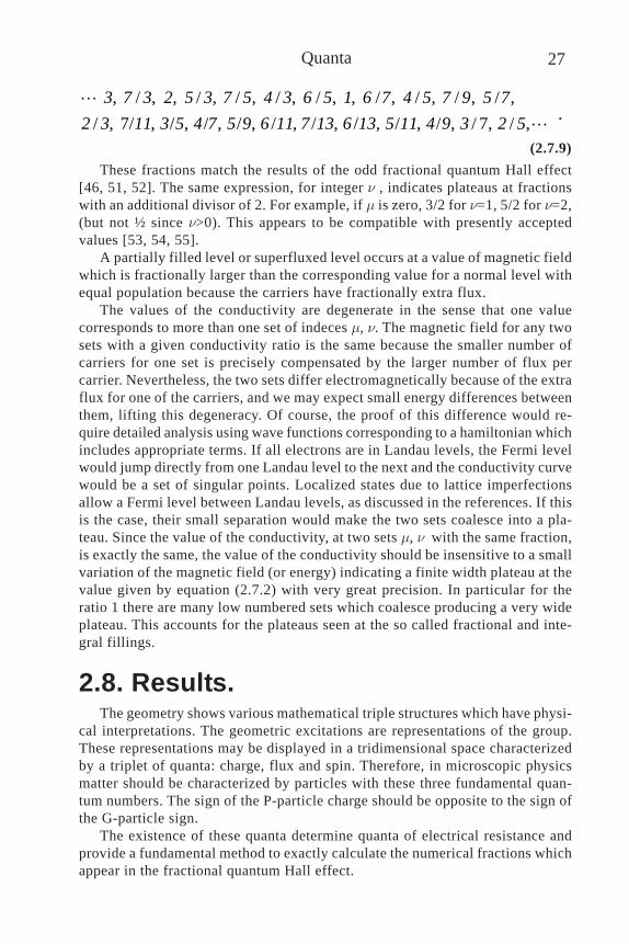
27Quanta
, / , , / , / , / , / , , / , / , / , / ,/ , 7/ , / , / , / , / , / , / , / , / , / 7, / ,
3 7 3 2 5 3 7 5 4 3 6 5 1 6 7 4 5 7 9 5 72 3 11 3 5 4 7 5 9 6 11 7 13 6 13 5 11 4 9 3 2 5
.
(2.7.9)These fractions match the results of the odd fractional quantum Hall effect
[46, 51, 52]. The same expression, for integer n , indicates plateaus at fractionswith an additional divisor of 2. For example, if m is zero, 3/2 for n=1, 5/2 for n=2,(but not ½ since n>0). This appears to be compatible with presently acceptedvalues [53, 54, 55].
A partially filled level or superfluxed level occurs at a value of magnetic fieldwhich is fractionally larger than the corresponding value for a normal level withequal population because the carriers have fractionally extra flux.
The values of the conductivity are degenerate in the sense that one valuecorresponds to more than one set of indeces m, n. The magnetic field for any twosets with a given conductivity ratio is the same because the smaller number ofcarriers for one set is precisely compensated by the larger number of flux percarrier. Nevertheless, the two sets differ electromagnetically because of the extraflux for one of the carriers, and we may expect small energy differences betweenthem, lifting this degeneracy. Of course, the proof of this difference would re-quire detailed analysis using wave functions corresponding to a hamiltonian whichincludes appropriate terms. If all electrons are in Landau levels, the Fermi levelwould jump directly from one Landau level to the next and the conductivity curvewould be a set of singular points. Localized states due to lattice imperfectionsallow a Fermi level between Landau levels, as discussed in the references. If thisis the case, their small separation would make the two sets coalesce into a pla-teau. Since the value of the conductivity, at two sets m, n with the same fraction,is exactly the same, the value of the conductivity should be insensitive to a smallvariation of the magnetic field (or energy) indicating a finite width plateau at thevalue given by equation (2.7.2) with very great precision. In particular for theratio 1 there are many low numbered sets which coalesce producing a very wideplateau. This accounts for the plateaus seen at the so called fractional and inte-gral fillings.
2.8. Results.The geometry shows various mathematical triple structures which have physi-
cal interpretations. The geometric excitations are representations of the group.These representations may be displayed in a tridimensional space characterizedby a triplet of quanta: charge, flux and spin. Therefore, in microscopic physicsmatter should be characterized by particles with these three fundamental quan-tum numbers. The sign of the P-particle charge should be opposite to the sign ofthe G-particle sign.
The existence of these quanta determine quanta of electrical resistance andprovide a fundamental method to exactly calculate the numerical fractions whichappear in the fractional quantum Hall effect.
3. Measurements and Motion.It is possible to give a geometrical representation to the postulates of quan-
tum mechanics. In most cases this is only a geometrical superstructure which maynot contain new physical ideas. On the contrary, it may be possible to start froma geometrical physical theory, and obtain its quantum implications. In this mannernew physical phenomena may arise.
Our theory considers excitacions of physical matter as representations of thestructure group of the geometrical theory. From this idea it follows that there arecertain discrete numbers associated with the states of microscopic matter. It wasshown that these numbers may be interpreted as quanta of angular momentum,electric charge and magnetic flux, providing a plausible explanation to the frac-tional quantum Hall effect (FQHE) [14 ]. The theory also leads to a geometricalmodel for the process of field quantization [56 ], implying the existence of fermionicand bosonic operators and their rules of quantization.We also presented [57] adefinition of mass in terms of the self energy of the nonlinear self interactionleading to the mass term in Dirac’s equation. It should be clear that a process ofphysical measurement should display these discrete geometric numbers as experi-mental quanta, leading to a particle (atomic) description of matter. It is necessary,therefore, to discuss the process of measurements within the physical geometry[23].
It may be claimed that, if the uncertainty principle is taken as fundamental, thegeometry at very short distances becomes a “fuzzy” geometry and the applica-tions of differential geometry is questionable. Nevertheless, nothing prevents us,within our theory, to continue taking differential geometry as fundamental, pro-viding the germ of quantum physics principles and represent particles by fluctua-tions or excitations around a geometric nonlinear substratum.
In particular, we consider the following questions: Can we define, within ourtheory, a geometric operation representing the process of physical quantum mea-surement? Are the results of this operation compatible with well known facts ofexperimental physics? Can we define and measure angular momentum and chargegeometrically?
We are also faced with the concept of mass. This concept plays a fundamental rolein relativity as shown by the relation between mass and energy and the principle ofequivalence between inertial and passive gravitational mass. From a relativistic pointof view, the rest mass of a system should be a unique concept defined in terms of theself energy of the system.
In quantum theory, a parameter in Dirac’s equation is interpreted as the relativisticrest mass, by means of the correspondence principle, This parameter is considered anunmeasurable number, bare mass, and a process of renormalization is required toinclude self energy effects in a corrected physical mass. Apart from the infinities thatappear in renormalization, there is no clear fundamentally derived relation betweenthese masses and a relativistic definition based entirely in terms of energy. We con-sider that such a relation is only possible within a unified theory.

29Measurements and Motion
Our physical geometry leads to the equations of relativistic quantum mechan-ics and it was shown in chapter 1 that it provides a bare inertial mass for a gener-alized Dirac equation [14, 58]. Since the nonlinear field equation of the theory andits integrability condition determine simultaneously the evolution of the field andthe motion of the sources, all self interaction effects are included in principle inany given solution. In other words, conceptually, it is not possible to have asolution for the field equation which does not satisfy the equations of motion ofthe sources. No additional self reaction forces are needed to describe the evolu-tion of field and source.
As in general relativity, [17 ] the self interaction difficulties arise when separat-ing the sources from the field while attempting an approximate solution. An ap-proximation (linearization) which splits these equations in an infinite system ofequations of different orders, requires the calculation of an infinite number ofcorrections due to self interactions. This renormalization is a consequence of themethod of approximation and not due to the nonlinear theory. In particular, it isalso possible to define and measure an inertial mass including self interactionwithout introducing unmeasurable bare masses.
3.1. Measurement of GeometricCurrents.
We shall study the properties of fluctuations or excitations of the geometricelements of the unified theory. If as suggested before [14], a particle may berepresented as an excitation of the geometry, its physical properties may be deter-mined by its associated fluctuations. These fluctuations may be characterizedmathematically by a variational problem. From a variational principle, if the equa-tions of motion hold, it is possible to define the generator of the variation. Thereis a canonical geometric current associated with this generator which geometri-cally represents the evolution or motion of the excitation, and should be consid-ered the subject of a physical measurement (observable).
The lagrangian density, in general, has units of energy per volume and theaction has units of energy-time. In the natural units defined by the connection(c=1, =1, e=1), the action is dimensionless. In the standard relativistic units(c=1), the constant arises as a factor in the action W.
It is well known that the variation of an action integral along a transformationof the variable y with parameters l is
RR
LW yd x Q d
ym
m¶
dd d d s
d= +òò 4 , (3.1.1)
where the canonical current , and the conjugate momentum P are defined by
dy dxQ L
d d
mm m md dl P dl
l l
æ ö÷ç ÷= = +ç ÷ç ÷çè ø , (3.1.2)

Chapter 3 ENERGY OR MASS AND INTERACTION30
,
Ly
m
m
¶P
¶= . (3.1.3)
The current is a geometrical object field which represents an observableproperty of a physical excitation, for example, angular momentum density. In gen-eral, a measurement is not a point process but rather it is an interaction excitationwith an apparatus over a local space-time region. In the geometric theory, theresults of a physical measurement should be a number depending on a variationalcurrent about a variation of a background section e, over a region R(m’) arounda characteristic point m on the base space M, with some instrumental averagingprocedure over the region. Therefore, we shall make the hypothesis that a mea-surement on a geometrical excitation is represented mathematically by a func-tional m of the observable geometric current defined by the associated variationover a complementary hypersurface s,
( ) ( ) ( ),m
R
m m m dmm
¶
s¢ ¢= ò . (3.1.4)
In some cases, excitations may be approximated as point excitations with noextended structure. In order to show the relation of our geometric theory to othertheories, without using any knowledge about the structure of excitations, we shalldefine a geometric measurement of a point excitation property by a process ofshrinking the region R(m’) of the current to the point m. With this procedure, thelocal section representing the excitation shrinks to a singular section at m. Wemay express this mathematically by
( ) ( )( )
lim m mR m m
d¢
= , (3.1.5)
where the functional dm is the Dirac functional.This process shrinks the current to a timelike world line. We may visualize the
boundary ¶R of region R as an infinitesimal cylindrical pillbox pierced by thecurrent at the bottom and top spacelike surfaces S. As the pillbox is shrunken topoint m, the functionals of the current dm() at the top and bottom surfaces areequal, if the current is continuous. The functional dm() on either of the spacelikesurfaces S is the geometric measurement.
From the lagrangian given for the theory [8, 9] the geometric current of anarbitrary matter excitation has the general form
e Xem mi= , (3.1.6)in terms of the frame e, an orthonormal set of the algebra i, the correlation on thespinor spaces ~, and the group generator X of the variation.
It should be noted that the frame e is associated with a set of states forming abase of a representation of the structure group. It does not represent a singlephysical state, but a collection of physical states. For any operator L in the alge-bra we may select, as the column vectors of the frame e, the eigenvectors f corre-sponding to L. Then we may write

31Measurements and Motion
( ) ( ), , , , ii ie eL L f f f l f l f l f l= = =1 2
1 2 1 2 , (3.1.7)
where l is the diagonal matrix formed by the eigenvalues li.Accordingly, the results of the measurement given by eq. (3.1.6), in coordi-
nates adapted to the 4-velocity u, is
( )m e Xe e ed i L= = =0 0 , (3.1.8)
which defines an associated operator L.In this expression, we should note e is the group inverse of e, and the corre-
lated product in the spinor space is a scalar. The product e e gives a unit matrix ofscalars, and the measurement values of the current coincide with the diagonalmatrix formed with its eigenvalues,
This result agrees with one of the postulates of quantum mechanics. Themathematical content of the last equation is truly independent of a physical inter-pretation of the frame e. In particular, it does not require, but allows that e is aprobability amplitude.
The result of the measurement essentially equals the value of the current atthe representative point m. Equivalently it is the average over a characteristic 3-volume V of S,
VV
Qd d
V V
mm
m md
s sdl
= = òò1 1 . (3.1.9)
This averaging, indicated by á ñ, is similar to the operation of taking the expec-tation value of an operator in wave mechanics.
The different generators of the group produce excitations whose propertiesmay be investigated by measuring the associated geometric currents. In particu-lar, we are interested here in currents associated with generators of the compactsubgroups, which were used to characterize the induced representations.
3.2. Geometric Spin.The concept of spin is related to rotations. In the geometric theory the com-
pact even generators form an su(2) subalgebra which is related to the rotationalgebra. The group homomorphism between this SU(2) subgroup and rotations is
( )†tra ab bR s s= 1
2 g g , (3.2.1)
where gÎSU(2) and RÎSO(3). The isomorphism between this SU(2) and the com-pact even subgroup of SL(2,) is the well known isomorphism between the com-plex numbers and a subalgebra of the real 2 ´ 2 matrices.
The isomorphism given by these expressions is not accidental, but is part ofthe conceptual definition of the geometric Clifford algebras as a generalization ofthe complex numbers and the quaternions. These algebras, and the spinor spaceson which they act, have well defined complex structures.
Chapter 3 ENERGY OR MASS AND INTERACTION32
If we consider that the generators kikj which belong to su(2) are the rotationgenerators, the associated geometric current is the angular momentum along thethird axis. For example, the result of the measurement of this current in a preferreddirection 3, using as illustration eq. (3.1.9) for the expectation value is
de dxd L
V d d
mm
ms Pl l
æ ö÷ç ÷= +ç ÷ç ÷çè øò3 1 , (3.2.2)
where the variation de is generated by k1k2. Then, for a flat metric,
ˆˆde de
d e u d xeV d V d
a mm as i i
l l= =ò ò3 3 01 1 . (3.2.3)
Since i0 commutes with k1k2 and i0i0 is -1, we identify the matrices and express thevariation generated by k1k2 as the differential of eq. (3.2.1). This rotation inducesa change in the functions on tridimensional space, giving a total variation for e of
( ) ( )y x y x
ie e x y e x y e
k kd ¶ ¶ dl s ¶ ¶ dl
æ ö æ ö÷ç ÷ç÷= + - = + - ÷ç ç÷ ÷ç ç÷ç è øè ø
1 23
2 2 , (3.2.4)
which leads to
( )( )y xd xe i x y eV
s ¶ ¶= - -ò3 3 312
1 . (3.2.5)
The factor ½ indicates, of course, that the SU(2) parameter l is half the angularrotation, due to the 2-1 homomorphism between the two groups.
This calculation was done, for simplicity, with only one component. It is clearthat if we use the three spatial components we get the expression for the angularmomentum vector operator L in quantum mechanics. The frame sections play therole of wave functions and the group generators play the role of quantum opera-tors. These similarities between our geometric theory and quantum mechanicsprovide essentially equivalent results. There are differences; in particular, wavefunctions have a complex structure and our frame sections have a Clifford struc-ture. Rather than a contradiction, this difference is a generalization, since thereare complex structures in different subspaces of the geometric Clifford algebra. Itis possible to introduce spaces of sections, but they certainly may have a struc-ture more general than a Hilbert space. The geometrical and group elements in thetheory actually determine many of its physical features.
3.3. Geometric Charge.The geometric source current J is a generalization of electric current. The
three compact generators k0, k5, and k1k2k3 are equivalent as electromagneticgenerators within the theory because there are automorphisms which transformany one of them into any other. It follows that the set ia, which enters into the

33Measurements and Motion
current, is defined up to an algebra automorphism. This allows us to take the i0
element as any of three electromagnetic generators without changing the physicalcontent of the theory.
The generalized source current J is the canonical current corresponding to avariation generated by an electromagnetic generator. In order to see this, we choosethe set km for im, and look for a variation generator which results in an automor-phism of the current. In other words, we look for a generator which gives anequivalent set to the set km by right multiplication. A generator which accom-plishes this is k5,
exp expm mp pk k k k k
æ ö æ ö÷ ÷ç ç= - ÷ ÷ç ç÷ ÷ç çè ø è ø5 5 5
4 4 . (3.3.1)
It is possible to find another one that results in a different automorphism but itwould lie in the electromagnetic sector. Thus it is clear that the current J corre-sponds to variations generated by the electromagnetic sector.
When we make a measurement of this canonical current J, we are measuringthe charge associated with the fluctuation of e related to a fundamental irreduc-ible representation of the group. We repeat the same calculation done in the pre-vious section for angular momentum current. If we neglect the gravitational part,the metric is flat, the expression for the measurement on the charged current is
ˆˆd e u ed
V Vm a m
m a ms k s= =ò ò1 1
(3.3.2)
where it is understood that we are working in the bundle SM which is the Whitneysum of the associated spinor vector bundle VM and its conjugate. Explicitly, interms of elements of VM the last equation is written as
eej d x
eV e
k kk k
-
-
é ù é ù é ùê ú ê ú ê ú= ê ú ê ú ê ú- ë ûë û ë û
ò1 0 5
315 0
00 0100 0
. (3.3.3)
It should be emphasized that the matrices in the last equation are 8´8 real matri-ces, the double-dimensional representation used in the SM bundle [9, 14]. The evengenerators may be written as 4´4 complex matrices using the isomorphisms men-tioned after eq.(3.2.1). We may substitute any equivalent generator for k0k5.
It is possible to choose a frame section e corresponding to eigenvectors of thefundamental representation of SU(2). In fact, since k5 commutes with k1k2, it isalso possible to choose a frame corresponding to common eigenvectors of thesetwo antihermitian generators belonging to the two su(2) subalgebras in sl(4,).The eigenvalues correspond to the quanta of spin and charge. Of course it isusual to work with the associated hermitian operators obtained by multiplicationby i, with real eigenvalues ± 1. Nevertheless the use of the antihermitian expres-sion is natural since they are generators of the two compact su(2) subalgebras
If e is an eigenframe of the generator, we get
j i= . (3.3.4)

Chapter 3 ENERGY OR MASS AND INTERACTION34
In other words, the result of this measurement for the fundamental repre-sentation is a quantum number equal to ±1. This conserved number may beinterpreted as the quantum of charge.
It is known that the electron charge plays two roles, one as the quantumof charge and the other as the square root of the fine structure couplingconstant a. In order to be able to reduce the theory to electromagnetism wemust account for Coulomb’s coupling constant k/4p and understand the rela-tionship of these constants. This k may be absorbed into the definition of thecurrent in eq.(1.2.2), but at the end it must be identified. It is better to show itexplicitly and to keep the frame e separate, as a section in the principal bundle,so that the conjugate e is the dual inverse of e, and the product e e is theunit matrix.
The dimensionless fine structure constant a is expressed in physical unitsas ke2/4pc. The units of the arbitrary constant k, which allows us to definethe electromagnetic units from the mechanical ones, are ml3t-2q-2. If we setk=4p, the units correspond to the gaussian system, where Coulomb’s con-stant is 1. If we set k=1, we obtain the Heaviside-Lorentz system whereCoulomb’s constant is 1/4p. If we set k=4pc210-7, we obtain the rationalizedMKSA system of units, where Coulomb’s constant is c210-7. In these sys-tems, the minimal coupling determines that the connection G corresponds toeA, in terms of the potential A and the electron charge e. On the other hand,rather than setting the value of k, it seems better to consider that the geomet-ric theory introduces a natural unit of charge by defining the electromag-netic potential, in energy units, equal to the connection. In this form the newgeometric unit of charge (the “electron”) equals e Coulombs, k is determinedto be 4pa and Coulomb’s constant becomes the fine structure constant a.With our definition of current and coupling constant (4pa) the calculatedcharge of the electron is ±1, in these geometric units. In arbitrary units, thecalculated quantum of charge e is ±(4pac/k)1/2.
In other words, this value is the minimum quantum of measurable chargechanges. This geometric prediction explains the two roles played by the elec-tron charge, as coupling constant and as quantum. In the previous sectionthe calculation lead to the well known values of angular momentum. In thissection we obtain a new theoretical result.
When there is only a U(1) electromagnetic field in flat space, our fieldequations reduce to [9]
d dA jpa* *= 4 . (3.3.5)
A particular solution for a static spherically symmetric potential A is
qA
ra
=0 , (3.3.6)
where q is the charge in “electrons”. If we now change our units to the gaussiansystem (1 electron = e coulombs), where a=e2 ,

35Measurements and Motion
2 (Gauss)A q qee
e er ra
j a= = = =0 , (3.3.7)
which is Coulomb’s law in terms of the charge qe in Coulombs.
3.4. The Concept of Mass.In relativity, the inertial rest mass of a particle is the norm of its four momen-
tum. In quantum mechanics, momentum is related to derivatives in space-time. Toshow the consistency of the concept of mass within our geometric theory, weshall consider the variation generated by a translation in the base space along theintegral curve of the vectors of the space-time tetrad ua. We obtain, in this way,four canonical geometric currents, as defined previously, whose average valuesover the volume V are
ˆ ˆedVm
a a mq P s= ò1 , (3.4.1)
where a indicates the four Lie derivatives with respect to the vectors ua and P isthe canonical momentum. In adapted coordinates we get
ˆ ˆ ˆe ed e ed xV V
ma a m aq k ¶ s k ¶- -= =ò ò1 1 0 31 1
. (3.4.2)
In particular, consider the trace of the time current and using the equation ofmotion assuming for the moment that e is constant, express the integral in terms ofthe connection Gm or potential,
ˆ trtr tr J d xe e d xV V
mmmm Gq k G-= =ò ò 31 3
0
1 1 . (3.4.3)
It is clear from the analogy with jmAm that JmGm should have the meaning of energyand that <q0> is the corresponding measured value. Furthermore we recognizethat the integrand in eq. (3.4.3) is in accordance with the fundamental mass-energyeq. (1.2.5). Later we shall come back to indicate the meaning of the conditionassumed.
This average energy leads to the concept of Dirac mass parameter for a par-ticle. It was pointed out above, that mass may be defined as a parameter related tothe potential. For geometrical reasons the unit of connection is inverse length, thesame as the operator ¶m. This provides a geometric (natural) unit of mass in termsof inverse length. Initially [14] we defined the mass parameter by
( )trm mmk G= 1
4 . (3.4.4)
It was noted that since we use time (length) as units of interval, the metric and itsrelated km matrix are dimensionless. Then the mass m has units of inverse length.

Chapter 3 ENERGY OR MASS AND INTERACTION36
We recognize now that a more general definition in accordance with section 1.3 is
( ) ( )tr trm e e Jm mm mk G G-= = =11 1
4 4 M (3.4.5)
which reduces to the previous one, eq. (3.4.4) under the simplifying assumptionsgiven previously.
The inertial mass of a particle is defined as a parameter related to a pair ofconnection and current which solve the nonlinear self interacting system. If thesign of the current in the source is changed it is conjectured that the sign of theconnection also changes and the mass remains positive. For an excitation aroundthe geometric inert substratum solution this nonlinear solution itself provides aparameter m0 for the linear excitation equation which may be considered the bareinertial mass parameter of the particle associated to the excitation.
Since the only element in the algebra with nonzero trace is the unit, we findthat
e e mImmk G- = +1 (3.4.6)
and we may write the equation of motion (1.2.7)
( )e e em mm m mk k ¶ G = - = 0 , (3.4.7)
as a Dirac equation,
e memmk ¶ = + . (3.4.8)
If we used the standard unit of mass, instead of the geometric unit, a constantappears in front of the differential operator, which is Planck’s constant . Thegeometric nature of Planck’s constant is determined by the connection in thesame manner that the geometric nature of the velocity of light c is determined bythe metric.
3.5. Invariant Mass.There is one difficulty with the given definition. The connection G is not a
tensor and under arbitrary change of reference frame the mass is not invariant [9].In words we may say that, in order to have an invariant mass, we must restrict thechange of the reference frame in such a way that the generator of the transforma-tion be orthogonal to the current J. For example, this would mean for standardelectrostatics that the scalar potential should not change in the transformation. Ifthe current J is odd, the mass given by eq. (3.4.5) is invariant under SL1(2,) andis, therefore, a Lorentz invariant.
Nevertheless, we realize that the theory applies to matter in the whole uni-verse. If a particle is associated to an excitation on a matter local frame in a dy-namic cosmic geometric background, we expect that the corresponding mass shouldbe related to the part of the connection responsible for the nonlinear local interac-tion with the local matter current.
37Measurements and Motion
It is convenient to separate the current into a part Jl corresponding to a localsystem representing a particle and another part Jb corresponding to the cosmicbackground which borders the system. The field equation in terms of the curva-ture takes the form,
( )t l bD J JW pa* * *= +4 , (3.5.1)
where Wt is the generalized curvature of the total connection Gt. If there is no localmatter, we have a background equation,
b bD JW pa* *= 4 , (3.5.2)
where Wb is the curvature of a cosmic background connection Gb.Far away from the region of the local material frame we may consider that its
effect is a small perturbation with respect to the dynamic cosmic background, butthis is not the case very close to a local material frame. In fact, close to it, thedynamic cosmic background may be considered a perturbation, with respect tothe nonlinear self interaction in the area of the tetrad section.
With this in mind, we may define the local material potential tensorial form Ll,the difference between the total and background connections,
l t bL G G= - , (3.5.3)
as the element responsible for the self energy of the interaction in the system.It is clear that a difference of connections is a tensor and that the last equation
is valid even in the case where the effect of the background is zero. In this case Gbwould be a flat inertial connection GI, which would be zero in some referenceframes but may have nonzero values in arbitrary reference frames. In general thisis not the case due to the presence of far away macroscopic matter.
The invariant expression for the mass is obtained from the total dynamic po-tential tensorial form L defined by eq. (1.3.2). Thus, we define
( )( )
( )( )
( )( )tr
trtr
C
l bC
J Jm J
I
m mm m m
m m
L LL L
k kº = = +
-140
0
g
g . (3.5.4)
This mass parameter is determined by the scalar product, using the Cartan-Killingmetric, of the potential and current which solve the nonlinear self interactingsystem. Since the Cartan-Killing metric depends on the representation [59] of thealgebra A used in the Dirac equation, the parameter m depends on the chosenrepresentation. In some representations the products involved are convolutionsrather than matrix multiplication.
If the background is negligible, Gb may be taken as a flat connection and thisequation reduces to the original one in those reference frames where Gb is zero.The extra mass like terms which appear in Dirac’s equation when an improperreference frame is used are similar to the inertial effects which appear in acceler-ated reference systems. These effects appear in eq.(3.4.8), apart from the mass, aspart of a “fictitious” inertial interaction. In fact, the flat GI related to the back-

Chapter 3 ENERGY OR MASS AND INTERACTION38
ground connection is called the inertial connection since it is the part responsiblefor all these inertial effects.
It should be noted here that a particle is associated to an excitation of thematter local frame in a very small region compared with the universe. The localmaterial frame is the dominant element and the dynamic cosmic background shouldbe treated as a perturbation which we consider negligible. We shall say that thelocal matter frame is the inert substratum for the excitation. In this case the sub-stratum is the dominant element, and the excitation should be treated as a linearperturbation on this nonlinear substratum solution. The value of the mass param-eter for the excitation should be related to the constant M associated to the inertsubstratum solution.
3.6. Equation of Motion.After justifying the identification of the parameter in eq. (3.4.4) as the inertial mass
we take a closer look at the geometric motion associated to the current J. Using thepotential relative to the inert substratum defined by equation (1.3.3), in inducedrepresentations, the new equation of motion (1.3.4) explicitly displays the termdepending on the invariant substratum mass, required by the Dirac equation,
( )
.
me e e e e e J
e me
m m mm m m m m m
mm
k k G k G
k
æ öæ ö- ÷ç ÷ç = ¶ - = ¶ - - ÷÷ç ç ÷÷çç ÷è øè ø
= - =
0
4
0
(3.6.1)
We now express all geometric objects by their even and odd parts. The geo-metric equation breaks in two complex equations for the even and odd parts of theG-system. We then designate different vector potentials in the connection with
the following notation: +Ai is the even part of the SU(2)Q sector ( )QG
of the
connection and corresponds to the electromagnetic potential; A is the comple-mentary odd part in the same sector; G is, in this section, the SL(2,) sector of theconnection which determines an L covariant derivative; is the complementarypart. Both -A and ¡ are complex matrices, respectively proportional to the iden-tity and the Pauli matrices, along the odd direction k0.
The odd and even parts of the frame, x and h, are elements of sl(2,) andsl(2,)Åu(1) respectively. The u(1) component contributes an overall phase andshould be neglected. Using conjugation the first equation may be written as
( )( ) † †i A i A mm m mm m m ms x s h s h ¡ h+ - + = + + . (3.6.2)
Similarly we get for the second equation
( )( ) ( ) ( ) ( )† †i A i A i i m im m mm m m m ms h h h G s x s x ¡ x+ -- ¶ + - = + - .
(3.6.3)
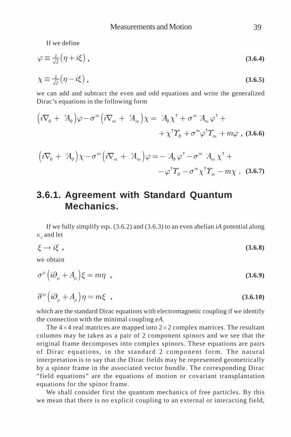
39Measurements and Motion
If we define
( )ij h xº +12 , (3.6.4)
( )ic h xº -12 , (3.6.5)
we can add and subtract the even and odd equations and write the generalizedDirac’s equations in the following form
( ) ( ) † †
† † ,
m mm m m
mm
i A i A A A
m
j s c c s j
c ¡ s j ¡ j
+ + - - + - + = + +
+ + +
0 0 0
0 (3.6.6)
( ) ( ) † †
† † .
m mm m m
mm
i A i A A A
m
c s j j s c
j ¡ s c ¡ c
+ + - - + - + = - - +
- - -
0 0 0
0 (3.6.7)
3.6.1. Agreement with Standard Quantum Mechanics.
If we fully simplify eqs. (3.6.2) and (3.6.3) to an even abelian iA potential alongk5 and let
ix x , (3.6.8)
we obtain
( )i A mmm ms ¶ x h+ = , (3.6.9)
( )i A mmm ms ¶ h x+ = , (3.6.10)
which are the standard Dirac equations with electromagnetic coupling if we identifythe connection with the minimal coupling eA.
The 4´4 real matrices are mapped into 2´2 complex matrices. The resultantcolumns may be taken as a pair of 2 component spinors and we see that theoriginal frame decomposes into complex spinors. These equations are pairsof Dirac equations, in the standard 2 component form. The naturalinterpretation is to say that the Dirac fields may be represented geometricallyby a spinor frame in the associated vector bundle. The corresponding Dirac“field equations” are the equations of motion or covariant transplantationequations for the spinor frame.
We shall consider first the quantum mechanics of free particles. By thiswe mean that there is no explicit coupling to an external or interacting field,
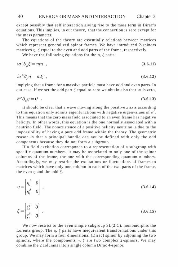
Chapter 3 ENERGY OR MASS AND INTERACTION40
except possibly that self interaction giving rise to the mass term in Dirac’sequations. This implies, in our theory, that the connection is zero except forthe mass parameter.
The equations of the theory are essentially relations between matriceswhich represent generalized spinor frames. We have introduced 2-spinorsmatrices h, x equal to the even and odd parts of the frame, respectively.
We have the following equations for the h, x parts:
i mmms ¶ x h= , (3.6.11)
i mmms ¶ h x= , (3.6.12)
implying that a frame for a massive particle must have odd and even parts. Inour case, if we set the odd part x equal to zero we obtain also that m is zero,
mms ¶ h = 0 . (3.6.13)
It should be clear that a wave moving along the positive z axis accordingto this equation only admits eigenfunctions with negative eigenvalues of s3.This means that the zero mass field associated to an even frame has negativehelicity. In other words, this equation is the one normally associated with aneutrino field. The nonexistence of a positive helicity neutrino is due to theimpossibility of having a pure odd frame within the theory. The geometricreason is that a principal bundle can not be defined with only the oddcomponents because they do not form a subgroup.
If a field excitation corresponds to a representation of a subgroup withspecific quantum numbers, it may be associated to only one of the spinorcolumns of the frame, the one with the corresponding quantum numbers.Accordingly, we may restrict the excitations or fluctuations of frames tomatrices which have only one column in each of the two parts of the frame,the even h and the odd x.
ˆ
ˆ
hh
h
é ùê ú= ê úê úë û
11
21
0
0 , (3.6.14)
ˆ
ˆ
xx
x
é ùê ú= ê úê úë û
11
21
0
0 . (3.6.15)
We now restrict to the even simple subgroup SL(2,C), homomorphic theLorentz group. The h, x parts have inequivalent transformations under thisgroup. We may form a four dimensional (Dirac) spinor by adjoining the twospinors, where the components h, x are two complex 2-spinors. We maycombine the 2 columns into a single column Dirac 4-spinor,
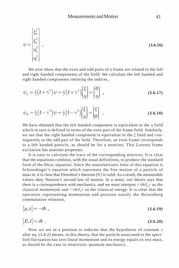
41Measurements and Motion
ˆ
ˆ
ˆ
ˆ
x
xy
h
h
é ùê úê úê úê ú=ê úê úê úê úë û
11
21
11
21
. (3.6.16)
We now show that the even and odd parts of a frame are related to the leftand right handed components of the field. We calculate the left handed andright handed components omitting the indices,
( ) ( )L
xy g y g
h h
æ ö æ ö÷ ÷ç ç= + = + ÷= ÷ç ç÷ ÷ç ç÷ ÷ç çè ø è ø5 51 1
2 2
01 1 , (3.6.17)
( ) ( )R
x xy g y g
h
æ ö æ ö÷ ÷ç ç= - = - ÷= ÷ç ç÷ ÷ç ç÷ ÷ç çè ø è ø5 51 1
2 21 10
. (3.6.18)
We have obtained that the left handed component is equivalent to the h fieldwhich in turn is defined in terms of the even part of the frame field. Similarly,we see that the right handed component is equivalent to the x field and con-sequently to the odd part of the field. Therefore, an even frame correspondsto a left handed particle, as should be for a neutrino. This Lorentz frameexcitation has neutrino properties.
It is easy to calculate the trace of the corresponding matrices. It is clearthat the equations combine, with the usual definitions, to produce the standardform of the Dirac equation. Since the nonrelativistic limit of this equation isSchroedinger’s equation which represents the free motion of a particle ofmass m, it is clear that Ehrenfest’s theorem [9 ] is valid. As a result, the measurablevalues obey Newton’s second law of motion. In a sense, our theory says thatthere is a correspondence with mechanics, and we must interpret <-ih¶m> as theclassical momentum and <-ih¶0> as the classical energy. It is clear that theoperators representing momentum and position satisfy the Heisenbergcommutation relations,
[ ],p x i= - , (3.6.19)
[ ],E t i= . (3.6.20)
Now we are in a position to indicate that the hypothesis of constant eafter eq. (3.4.2) means, in this theory, that the particle associated to the speci-fied fluctuation has zero lineal momentum and its energy equals its rest mass,as should be the case in relativistic quantum mechanics.
Chapter 3 ENERGY OR MASS AND INTERACTION42
3.7. Results.Measurements on geometric excitations determine integral expressions similar
to the expectation values in quantum mechanics. These expressions display thetriple structure of charge, flux and spin quanta. The associated operators satisfythe Heisenberg commutation relations. In fact, it appears that this geometry is thegerm of quantum physics including its probabilistic aspects. The mass may alsobe similarly defined in an invariant manner in terms of energy, depending on thepotential and matter current. The equation of motion is a geometric generalizationof Dirac’s equation. The geometric nature of Planck’s constant h and of lightspeed c is determined by their respective relations to the connection and themetric.
4. Masses.The fundamental dynamic process in the theory is the action of the connec-
tion or potential on the frame. Since the connection is valued in the Lie algebra ofthe group G and the frame is an element of G, the dynamic is realized by the actionof the group on itself. The principal bundle structure [36] of the group, (G,K,L),provides a natural geometric interpretation of its action on itself. A particularsubgroup L defines a symmetric space K, the left coset G/L, the base space of thebundle. The subgroup L, the fiber of the bundle, acts on itself on the right, andalso is the isotropy subgroup of the coset K. The complementary coset elementsact as translations on the symmetric coset.
This geometric interpretation may be transformed into a physical interpreta-tion if we choose L to be homomorphic to the spinor group, SL(2,), related to theLorentz group. The action of L is then interpreted as a Lorentz transformation(pseudorotation) of the external space, the tangent space TM of the physicalspace-time manifold M, defining its metric. The action of the complementary cosetK is interpreted as a translation in the internal space, the symmetric coset K itself.There is then a nontrivial geometric relation between the internal and externalspaces determined by the Clifford algebra structure of the manifold. The space Kis the exponentiation of the odd sector of the Clifford algebra and is related tolocal copies of the tangent space TM and its dual cotangent space T*M. It may beinterpreted as a generalized momentum space. The states of momentum k wouldcorrespond to the points of K.
It follows that the frame excitations are also acted by the potential and evolveas representations of G. The constant parameter m characterizes an eigenvalue ofa differential operator , defined by the equation of motion, acting on excitationsde of a substratum solution over a locally symmetric space-time, seen by somedefinite observer and therefore m also characterizes the eigenvalue of the qua-dratic differential operator 2 on space-time.
Different observers would measure different relative momenta k for a givenexcitation. A measurement for each k corresponds to a function in momentumspace. An abstract excitation is an equivalence class of these functions, under therelativity group. Since the group space itself carries its own representations, therealization of excitations as representations defined on the group space have afundamental geometric character. The geometric action of the K sector is a trans-lation on itself and the functions on K are the internal linear representations thatmay be observed (observables). The action of the L sector is a Lorentz transfor-mation and sl(2,) spinors are the observable external representations. For thesereasons, we must represent physically observable excitations by classes of spinorvalued functions on the symmetric K space. In particular, we realize them on avector bundle, associated to the principal bundle (G,K,L), taking as fiber the sl(2,)representation valued functions on the symmetric K space. Essentially, this is, infact, done in particle physics when considering representations of the Poincaregroup.Our representations are representations of SL(4,) induced from SL(2,).

Chapter 4 ENERGY OR MASS AND INTERACTIONS44
It was indicated in chapters 1 and 2 that the base manifold, the space-time M,is a manifold modeled on K. Given an observer, the excitations on M may be locallyidealized as functions on the symmetric space K locally tangent to M at a point uin an a neighborhood UÌM. For the moment we restrict G to its 10 dimensional Psubgroup. The tangent symmetric model space is isomorphic to the hyperbolicspace P/L which has a LaPlace-Beltrami differential operator corresponding to thequadratic Casimir operator 2. Because of the local isomorphism between the tan-gent spaces of M and P/L, we may take 2 as the corresponding space-time imageof 2.
The constant m would then characterize the eigenvalues of 2. It is known thatthe representations of P induced on P/L are characterized by the eigenvalues ofthis Casimir operator [60, 36] and therefore they would also be characterized by m.In general we would then have that the parameter m associated to an excitation(wave) function on M, as seen by some definite observer, characterizes an in-duced representation of G on G/L. Because of this pure geometric relation be-tween the 2 and 2 operators the induced representations should play a signifi-cant physical role. It should be clear the geometrical origin of this well knownphysical hypothesis in elementary particle physics.
Choosing a particular induced representation of G on G/L and definite localobservers in a neighborhood around a given point in M determines the excitation(wave) function. Since we deal with a class of relativistic equivalent observers, weactually have a class of (wave) functions on M, one for each transformation link-ing valid observers. The section of the fiber bundle E defining a particular in-duced representation has for support the mass hyperboloid in K characterized bythe rest mass value m. Once we have chosen observers at points u in a neighbor-hood U in M, corresponding to points k on the mass hyperboloid, we have (wave)functions on M with definite values of k(u) in the neighborhood U. The isotropygroup of the mass hyperboloid, the one that leaves a point (momentum) invariant(“little” group), transforms the (wave) functions on the mass hyperboloid. If wehave the flat trivial bundles used in standard quantum theories, for example, if Mis flat Minkowski space, P is the Poincare group and L is the Lorentz group thenthe quotient P/LK is a flat Minkowski (momentum) space distinct but isomorphicto (space-time) M and the little group on the mass hyperboloid in K is SO(3) orISO(2). The (wave) function becomes the standard particle wavefunction depend-ing on a single definite value of k throughout M.
Due to the preceding arguments, when we try to calculate the physical valuesm, corresponding to excitations on a substratum, we must use the induced repre-sentations characterized by m, which are the ones that represent geometric excita-tions of definite momentum k by (wave) functions on space-time, carrying geo-metrical and physical significance.
From our geometric point of view, it has been claimed [61 ] that the proton, theelectron and the neutrino are representations of SL(2,) and its subgroups, in-duced from the subgroups SL1(2,) and SL(2,). This is a generalization of par-ticles as representations of the Poincare group induced from its Lorentz subgroup[62]. Using our definition of mass [57, 63], it is possible to find an expression forthe mass of these geometric excitations and compare them with the proton elec-

45Masses
tron mass ratio (a not fully explained geometrical expression is known [64, 65, 66]).It should be noted that there is no contradiction in this calculation with presentphysical theories, which may be considered as effective theories derived undercertain conditions and limits from other theories. The structure group G of thetheory, SL(4,), has been used in an attempt to describe particle properties [67, 68,69] in another approach.
These results ratify that quantum mechanics effects may be contained in theunified theory. A curved substratum may also be a mechanism to give masses tothe potential excitations. This is only possible for nonlinear theories like the oneunder discussion and is interesting, since we have found a simple inert substra-tum solution to the nonlinear field equation. Here we find particular equations forthe case of a potential field excitation around this substratum solution [63]. Inaddition we will discuss under what conditions the excitations are massless.
4.1. Bare Inertial Masses for FrameExcitations or Fermions.
The definition of the mass parameter m, in terms of a connection or potentialon the principal fiber bundle (E, M, G), has been given in the fundamental definingrepresentation of SL(4,) in terms of 4´4 matrices, but in general, may be writtenfor other representations using the Cartan-Killing metric Cg [70], defined by thetrace. The definition of this metric may be extended to the Clifford algebra A,which is an enveloping algebra of both sl(4,) and sp(4,). The Clifford algebra Ais a representation and a subalgebra of the universal enveloping algebra U ofthese Lie algebras. We have normalized the mass, within a fixed group representa-tion, by the dimension of the vector space carrying the representation, given bythe trace of the representative of the identity in A. We may write the definition ofthe mass parameter from eqs. (1.2.5) or (3.5.4) in any representation of the algebrassl(4,) and sp(4,) and the corresponding representation of the common envel-oping Clifford algebra (A) as
( )( )( )
( ) ( )( )( ) ( )( )
trtrtr
tr tr
C
00
g14 g
C
A A
J JJm J
I I
mmmmm
m
G GGG
k k= = º =
-
. (4.1.1)
It is known that the Cartan metric depends on the representations, as indicated insection 3.5, but we shall only apply this expression to find ratios within a particu-lar fixed induced representation of the enveloping algebra.
If we consider geometric excitations on a substratum, this mass may be ex-panded as a perturbation around the substratum in terms of the only constant ofthe theory, the small fine structure parameter a characterizing the excitation,
J J J Ja a= + + +20 1 2 , (4.1.2)
G G aG a G= + + +20 1 2 , (4.1.3)

Chapter 4 ENERGY OR MASS AND INTERACTIONS46
( )( )trm J J Jm m mm m mG a G a G a= + + + 2
0 0 1 0 0 114
, (4.1.4)
indicating that the zeroth order term, which we shall call the bare mass, is givenentirely by the substratum current J0 and connection G0, with corrections depend-ing on the excitation self interaction.
The variation of J is orthogonal to J. In the same manner as the 4-velocity hasunit norm in relativity and the 4-acceleration is orthogonal to the 4-velocity, wehave in the defining representation of tetradimensional matrices,
G G H H G G H HJ J e ee e I J J J J J Jmmk k- -· · · ·¢ ¢ ¢ ¢= = - = = =1 1 4 . (4.1.5)
This implies that J1 is orthogonal to J0,The first order mass correction is
( ) ( )tr tr trgm J J m J J J Ja a a
D G G G G· · · · ·= + = + =1 0 0 1 1 0 0 1 0 14 4 4 .
(4.1.6)The first order equation for the potential is linear, expressed using a linear differ-ential matricial operator. If we take the projection along J0, its source becomes zeroand since J0 is constant there are no Dm solutions that depend physically on thesource J. It follows that the first order correction must be zero and the masscorrection should be of order a2, or 10-5. These corrections correspond to a geo-metric quantum field approximation (QFT) [56 ]. In this section we limit ourselvesto the zeroth order term which we consider the bare mass of QFT.
The structure group G is SL(2,) and the even subgroup G+ is SL1(2,). Thesubgroup L is the subgroup of G+ with real determinant in other words, SL(2,).There is another subgroup H in the group chain GÉHÉL which is Sp(2,). Thecorresponding symmetric spaces and their isomorphisms are discussed in a previ-ous publication [63]. We are dealing with two quotients which we shall designateas C and K,
( , ) ( , )( , ) ( ) ( , ) ( )
G SL SOK
G SL SO SO SO+
º @ @Ä Ä
4 3 32 2 3 1 2
, (4.1.7)
( , ) ( , )( , ) ( , )
H Sp SOC
L SL SOº @ @
4 3 22 3 1 . (4.1.8)
These groups have a principal bundle structure over the cosets and themselvescarry representations. The geometric action of the K generators are translationson the coset K. The functions on K are the natural internal representations.
We shall consider, then, the representations of SL(2,) and Sp(2,) inducedfrom the subgroups SL1(2,) and SL(2,) over the symmetric spaces SL(2,)/SL1(2,) and Sp(2,)/SL(2,), respectively. These geometric induced
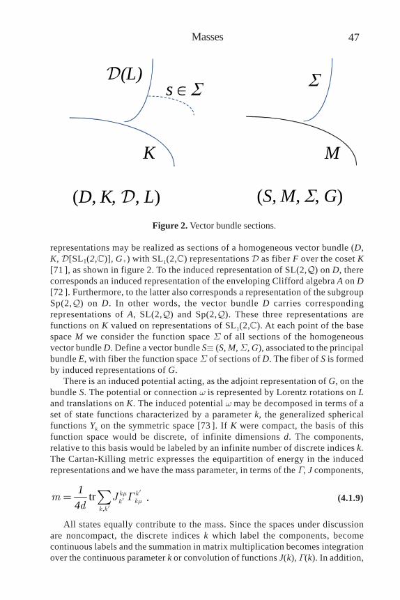
47Masses
representations may be realized as sections of a homogeneous vector bundle (D,K, [SL1(2,)], G+) with SL1(2,) representations as fiber F over the coset K[71 ], as shown in figure 2. To the induced representation of SL(2,) on D, therecorresponds an induced representation of the enveloping Clifford algebra A on D[72 ]. Furthermore, to the latter also corresponds a representation of the subgroupSp(2,) on D. In other words, the vector bundle D carries correspondingrepresentations of A, SL(2,) and Sp(2,). These three representations arefunctions on K valued on representations of SL1(2,). At each point of the basespace M we consider the function space S of all sections of the homogeneousvector bundle D. Define a vector bundle Sº (S, M, S, G), associated to the principalbundle E, with fiber the function space S of sections of D. The fiber of S is formedby induced representations of G.
There is an induced potential acting, as the adjoint representation of G, on thebundle S. The potential or connection w is represented by Lorentz rotations on Land translations on K. The induced potential w may be decomposed in terms of aset of state functions characterized by a parameter k, the generalized sphericalfunctions Yk on the symmetric space [73 ]. If K were compact, the basis of thisfunction space would be discrete, of infinite dimensions d. The components,relative to this basis would be labeled by an infinite number of discrete indices k.The Cartan-Killing metric expresses the equipartition of energy in the inducedrepresentations and we have the mass parameter, in terms of the G, J components,
,
tr k kkk
k k
m Jd
mmG ¢
¢¢
= å14
. (4.1.9)
All states equally contribute to the mass. Since the spaces under discussionare noncompact, the discrete indices k which label the components, becomecontinuous labels and the summation in matrix multiplication becomes integrationover the continuous parameter k or convolution of functions J(k), G(k). In addition,
Figure 2. Vector bundle sections.
(S, M, , G)
M
s (L)
(D, K, , L)
K
Chapter 4 ENERGY OR MASS AND INTERACTIONS48
if we work with tetradimensional matrices and continuous functions on the cosetK, the Cartan-Killing metric in A is expressed by trace and integration, introducinga 4V(KR) dimension factor for the common representation space D, giving
( )( ) ( )tr , ,
R
dkm J k k k k dkV A
G= ò ò 2 2 21
4 . (4.1.10)
where V(AR) is a characteristic volume determining the dimension of the continuousrepresentation of A. We interpret the value of a function at k as the componentwith respect to the basis functions Y(kx) of the symmetric space K, parametrizedby k, as usually done in flat space in terms of a Fourier expansion. We may saythat there are as many “translations” as points in K. It should be noted that these“translations” do not form the well known abelian translation group.
The G-connection on E induces a SO(3,1)-connection on TM. The combinedaction of the connections, under the even subgroup G+, leaves the orthonormalset km invariant [9] , defining a geometric relativistic equivalence relation R in theodd subspace K. Each element of the coset is a group element k which correspondsto a space-time moving frame. Physically a class of equivalent moving frames k isrepresented, up to a boost transformation, by a single rest frame, a point k0 whichcorresponds to the rest mass m0.The decomposition of G and J over the coset K isinto equivalence classes of state functions Y(kx). The number of classes of statefunctions Y(kx) (independent bases), is the volume of a subspace KRÌK of classes(nonequivalent points under a relativistic boost transformation integral I(b)).Physically the integral represents summation of the potential ´ current product,over all inequivalent observers, represented by a rest observer.
There is a constant inert substratum solution [74 ], discussed in section 1.3, for thenonlinear differential equations that provides an SL(2,) valued 1-form inert potentialL to the principal fiber bundle (E,M,G). The only contribution of eq. (4.1.10) to theinert rest mass m0 is through L which represents the class of equivalent local potentialforms G. At some particular frame s, which we may take as origin of the coset, the localexpression for L is constant.
All points of K or C may be reached by the action of a translation by k,restricted to the corresponding subgroup, from the origin of the coset. As thereference frame changes from s at the origin to sk at point k of the coset, the localpotential form changes as eq. (1.3.2), corresponding to the equivalence class ofconstant solutions L. All changed potentials correspond to the same constantsolution class L, seen in the different reference frames of the coset.
In the principal bundle the constant potential L combines with the constant Jto produce a constant product over the coset K as shown in section 3.5. Asindicated before, the mass variation produced by the last term in the equation,due to an arbitrary choice of frame, corresponds to inertial effects. The dominantnoninertial effects are due to the first term in the right hand side of the equationbecause the current J is a tensorial form which corresponds to the substratumpotential tensor L. It is clear that the subtraction of L from the potential, the lastterm in the equation which only has a frame k dependence, transforms as aconnection, and corresponds to the inertial connection. The physical contribution

49Masses
to the bare mass parameter may be calculated in terms of L, in the special frame s,defining an invariant expression in the group G and its subgroups valid for agiven representation.
We are interested in the representations of SL(2,) and Sp(2,) induced bythe same representation of SL1(2,) and corresponding to the same inert substratumsolution. In the defining representation of tetradimensional matrices, the productJJ contained in the LJ term is
G G H H G G H HJ J e ee e I J J J J J Jmmk k- -· · · ·¢ ¢ ¢ ¢= = - = = =1 1 4 , (4.1.11)
invariant under a SL(2,) transformation on coset K and equal to the unit in thealgebra A for both the G group and any H subgroup. There is a representation ofA on the bundle S corresponding to the induced representation. The invariance(equality) of the product JJ must be valid in any representation of A, although thevalue of the product may differ from one representation to the other. For theinduced function representations valued in the sl(2,) algebra (Pauli matrices),the invariant product becomes the k integration,
( ) ( ) ( )
( ) ( )
ˆˆˆ ˆ
ˆˆˆ ˆ
,, ,
, ,
FF k kJ k k J k k dk
J k k J k k dk
a m bm a b
a m bm a b
k k k k
k k k k¢
=º =
¢ ¢ ¢ ¢ ¢
ò
ò
001 301 2 2 3 2
0201 2 2 3 , (4.1.12)
which, must be a constant 4´4 matrix F0 on K, independent of k1 and k3.The trace expression for the mass becomes
( )( )tr ,
RKR
F k k dkmAV
= òM . (4.1.13)
The integrand is the same F0 constant for both groups, but the range ofintegration KR differs. Integration is on a subspace KRÌK of relativistic boostinequivalent points of K for the group G and on a subspace CRÌCÌK for thegroup H. The expressions for the masses corresponding to G-excitations andH-excitations become,
( )( ) ( )
( )( )tr,tr
R
RG
KR R
V Km FF k k dkV A V A
= =ò 0M
M , (4.1.14)
( )( )
( )( ) ( )
( )( )
tr,trR
G RH R
C RR R
m V CFm F k k dk V C
V KV A V A== =ò 0
MM.
(4.1.15)

Chapter 4 ENERGY OR MASS AND INTERACTIONS50
The bare mass parameters m are related to integration on coset subspaces,depending proportionally on their volume. In other words, the ratio of thebare mass parameters for representations of SL(2,) and Sp(2,), inducedfrom the same SL(2,) representation as functions on cosets K and CÌKshould be equal to the ratio of the volumes of the respective subspaces. Thevalues of mass are related by the equation
( ) ( )
( ) ( )
tr tr
tr tr
m J J
e e e e I
m mm m
mm
G L
k k- -
= =
æ öæ ö- ÷ç ÷ç= = =÷÷ç ç ÷÷çç ÷è øè ø
1 14 4
1 11 14 44
MM M . (4.1.16)
4.2. Symmetric Cosets.
4.2.1. Volume of C Space.First consider, the volume of the tetradimensional symmetric space Sp(2,)/
SL(2,) which coincides with the quotient SO(3,2)/SO(3,1). In the regularrepresentation, it has the matricial structure determined by the groups [75, 76]. Inparticular the volume of C is obtained by an integration over this curvedminkowskian momentum space using coordinate relations given by the group. Wesplit the integration into the angular integration on the compact sphere S2, theradial boost b and the energy parameter c,
( )
( )2
sin sinh
sinh C
V C dd d
d I
b pp
b
Wc c b b
p pb b b
= =
=
ò ò ò
ò
4
23 2
0 0 0
0
16 163 3
, (4.2.1)
obtaining the result in terms of a boost integral I(b).
4.2.2. Volume of K space.For the volume of K, the integration is over an 8 dimensional symmetric space.
This space G/G+ has a complex structure and is a nonhermitian space [77]. Usingits complex coordinates we define an equivalence relation S in the points on K bydefining equivalent points as points with equal coordinate moduli,
S S S S S= ´ ´ ´1 1 1 1 . (4.2.2)The volume of K will then be the product of the volumes of S and the volume
of the coset K/S. We split the integration into the integration on the 4 compactphase spaces S and integration on the tetradimensional coset space K/S,

51Masses
parametrized by the coordinate moduli. The last integration is further split intointegration on the compact 3 spheres S3 and integration on the complementarynoncompact direction, which corresponds to boosts b, obtaining
( ) ( ) ( )/
sinh sin
K
d d d d d V K S V Sg VV K
dd d db pp p
y y y y
yb b Wz z
´- == =
æ ö÷ç ÷ç´ ÷ç ÷÷çè ø
ò
ò ò ò ò
40 1 2 3
4243 2 3
0 0 0 0
, (4.2.3)
( ) ( )( ) ( )sinh KdV K Ib
p p b b p b= =ò42 3 5 6
0
2 2 2 , (4.2.4)
in terms of another boost integral I(b). This result shows, as should be expected,that the relativistic equivalent subspace of K is of higher dimension than therelativistic equivalent subspace of C, as indicated by the respective integrals ofthe hyperbolic sine of b.
4.2.3. Ratio of Geometric VolumesWe expect that the ratio of the volumes V of the inequivalent subspaces of K
and C, corresponding to fundamental representation of spin ½, should be relatedto the ratio of the corresponding geometrical masses. We have to eliminate theseequivalent points by dividing by the equivalence relation R under the boosts ofSO(3,1). Equivalent points are related by a Lorentz boost transformation ofmagnitude b . There are as many equivalent points as the volume of the orbitdeveloped by the parameter b.
The respective inequivalent volumes are, for C,
( ) ( )( )( )
( )
( )C
RC
IV CV C
IV R
pb p
bb= = =
16163
3 , (4.2.5)
and for K,
( )( )
( )( )( )
( )K
RK
V K IV K
IV R
p bp
bb= = =
5 65 62
2 . (4.2.6)
Although the volumes of the noncompact spaces diverge the ratio of the compactsubspaces, taking in consideration the equivalence relation R, has a well definedlimit, obtaining

Chapter 4 ENERGY OR MASS AND INTERACTIONS52
( )( )
R
R
V K
V Cp= 56 . (4.2.7)
We actually have shown a theorem which says: The ratio of the volumes of Kand C, up to the equivalence relation R under the relativity subgroup, is finiteand has the value 6p5 .
4.3. The p, e and n Mass Ratios.For a constant solution, the masses are proportional to the respective volumes
V(KR). The constants of proportionality only depend on the specified inducingSL(2,) representation. In particular for any two representations induced from thespin 1/2 representation of L, the respective constants are equal.
Using the theorem of the previous section, the ratio of bare masses of thefundamental representations of the groups G and its subgroup H induced fromthe spin 1/2 representation of L, for the constant solution, equals the ratio of thevolumes of the inequivalent subspaces of the respective cosets G/L1 and H/L, andhas the finite exact value
( )( )
. .pRG
H R e
mV Kmm V C m
p= = = » =56 1836 1181 1836 153 , (4.3.1)
which is a very good approximation for the experimental physical proton electronmass ratio, in confirmation of the relation of the G group to the proton and the Hgroup to the electron. The only other physical subgroup L=SL(2,) of G shouldlead to a similar mass ratio. Previously we have related L to the neutrino. In thiscase the quotient space is the identity and we get
( )( )
( )( )
/R RL
H R R e
V L L V Im mm V C V C m
n= = = =0 , (4.3.2)
which is in accordance with the zero bare mass of the neutrino. The physical massof the neutrino may include a small correction term due to the excitation.
4.4. The Equation for the PotentialExcitations or Bosons.
We consider now the equations for the geometric potential excitations aroundthe fixed substratum geometry. In a particular case we shall show that the excitationequations take the form of a Yukawa equation. The corresponding solutionsbehave as short range fields, with a range given by a constant associated to thesubstratum potential solution. This constant, which in general depends on theparticular representation, may also be interpreted as the mass of the particleassociated to the potential excitation.

53Masses
The field equation of the theory,
D JW pa* *= 4 , (4.4.1)is expanded [78] by writing the exterior product in terms of differential forms andgroup generators. The expression for the field equation becomes
( ) ( )[ ]
[ ] [ ][ ]
[ ]
,
, , ,
a a ba a bg g
a b c a b aa b c a b a
gg g E g E E
g g E E E E E J E
rm an r ar m n r
rm an r a ar m n r
¶ ¶ w ¶ w w
w ¶ w w w w pa
- -- + - +
é ù+ =ë û
2 1
2 4 .
(4.4.2)The commutator in the expressions introduce the structure constants and thetrace of products of the Lie algebra base introduces the Cartan-Killing metric.
We shall proceed formally in the defining 4´4 representation. The equationmay be written in terms of components referred to these bases. We note that theterms quadratic in the structure constant also include terms depending on theCartan-Killing metric. This may be seen from the trace expression.
To obtain field excitations we perform perturbations of the geometric objectsin the equation. Then the linear differential equation for the perturbation of thepotential takes the general form
( )[ ]
cd c dg
cd c d d
gg g
L L g J
rm an r ar m n r
a r amn ar mn
¶ ¶ dw w w dw
dw d pad
-- +
+ + =
2
1 2
4
4 , (4.4.5)
where 1L and 2L are linear first and second order operators, respectively, withvariable coefficients which are functions of w . The second term, which arisesfrom the cubic self interaction term, may provide a mechanism to give effectivemasses to the potential excitations in the curved substratum, in terms of a param-eter which represents the self energy determined using the Cartan-Killing metricin the defining representation,
ccr
rw w w=2 . (4.4.6)
4.5. Massive Particular Solutions.We have constructed a pair of conjugate constant complex substratum solu-
tions [78], in terms of the geometrical fundamental unit of energy M, by extendingthe real functions in eq. 1.3.2 for the substratum to complex functions,
( ) ( )ˆ ˆˆ ˆ ˆdx dx ia aa a aw k k k k= - = - 5 4 1 4 M M . (4.5.1)
In particular if we assume that we can obtain a potential solution with alge-braic components only in the complex Minkowski plane Kk generated by the Cliffordalgebra orthonormal set k, we have that the complete base E may be replaced bythe orthonormal set k . Since the potential has no even components, the metric in

Chapter 4 ENERGY OR MASS AND INTERACTIONS54
the base space-time M is flat. Using the trace relations we obtain the excitationequation using the complex metric g of the complex Minkowski plane Kk, whichinvolves lowering the indices and taking the complex conjugate,
( )( )
ˆ ˆ ˆˆ ˆ ˆ ˆ ˆ ˆˆ
ˆ ˆ ˆ ˆˆ ˆ ˆ ˆ
d d
J
n c ar bn c ar bn c ar bnr r rd
nca ddb da cb
dw dw w w w dw w w w dw
pad
* * + + + ´
- =
4
g g g g 4 , (4.5.2)
ˆˆ ˆ ˆ ˆd d Ja a r a a
rd d d ddw w dw w dw d pad* * + + =
2 22 4 . (4.5.3)
Given a representation, a solution to these coupled linear equations may al-ways be found in terms of the Green’s function of the differential operator and thecurrent excitation dJ, which may be an extended source. In order to decouple theequations, it is necessary to assume that dwr
r vanishes. If this is the case then allequations are essentially the same and the solution is simplified.
We shall restrict ourselves to consider the equation for a unit point excitationof the quantum of physical charge and its solution which is the Green’s function.If we assume a time independent excitation with spherical symmetry, the onlyrelevant equation would be the radial equation. Since M is constant, it representsan essential singularity of the differential equation, an irregular singular point atinfinity. The corresponding solutions have the exponential Yukawa [79] behavior.Let us interpret that the curved substratum gives an effective range w-1 to thelinear excitations. Equation (4.5.3) when time independent for a point source be-comes, designating the fluctuation as a weak field W,
( ) ( ) ( )W x W x g x xw pa d ¢- + = -2 2 2 24 , (4.5.4)
where we explicitly recognize that the current is of order a or equivalently of ordercharge squared. Furthermore, we realize that the assumed excitation is the odd partof an su(2)Q representation and should explicitly depend on the formal odd part of thecharge. The charge which enters in this first order perturbation equation is thesu(2)Q charge, eq. (3.3.4), defined by the original nonlinear unperturbed equation.This is the quantum of the only physical charge: the electric charge quantum e=1. Weshould define a factor g to expresses the geometric charge quantum in units of anundefined formal odd charge (or weak charge). The a and g factors are not part of thed function which represents a unit odd charge. This equation may be divided by(ag)2, obtaining the equation for the odd excitations W produced by the unit oddpoint charge or equation for the Green’s function
( )( ) ( ) ( )W x W x x x
gg
wpd
aa
æ ö÷ç ¢ - = - -÷ç ÷÷çè ø
22
21 4 . (4.5.5)
We may define a new radial coordinate r=agx’, rationalized to a new range -m-1 forodd excitations, which incorporates the ag constant. Taking in consideration the

55Masses
covariant transformations of the function W and Dirac’s d, the radial equation isthen
( ) ( )rW W r rr r
¶m pd
¶- ¢- = - -
22
21 4 . (4.5.6)
Since -m is constant, the Green’s function for this differential operator is
x x re ex x r
m m
p p
- -¢- - ¢-
= =¢ ¢-
1 14 4
. (4.5.7)
whose total space integration introduces, in general, a range factor,
r ddr r e
p
m Wp m
-
¥
¢--
¢¢ ¢ =òò4
22
00
1 14
, (4.5.8)
The range -m may be evaluated using eqs. (4.5.1) and (4.5.3),
( ) trCCm m
m mw w w w w*= = =2 214g 2M , (4.5.9)
obtaining
g g
wm
a a- = =
2M
. (4.5.10)
In order to obtain a complete excitation, instead of only its odd part, set gequal to 1.
4.6. Massive SU(2) Bosons.According to physical geometry we may consider excitations of the SU(2)Q
subgroup of G around the substratum. The complex substratum solution indi-cates that this excitation acquires an effective mass. Let us consider the threecomponents of an SU(2)Q potential A as three classically equivalent electromag-netic potentials.
The electromagnetic subgroup is SU(2)Q, similar to the spin subgroup SU(2)S.The group itself, as a fiber bundle (SU(2),S2,U(1)) carries its own representations [78,80]. The base space is the coset SU(2)/U(1) which is the bidimensional sphere S2.The fiber is an arbitrary even subgroup U(1). The action of this electromagneticSU(2)Q is a multiplication on the fiber by an element of the U(1) subgroup and atranslation on the base space S2 by the action of the SU(2)Q group Casimir opera-tor, representing a squared total SU(2)Q rotation.
This action is not as simple as translations in flat spaces, but rather has com-plications similar to those associated with angular momentum due to the SU(2)group geometry. The orientation of directions in SU(2) is quantized. In particularonly one component of the electromagnetic rotation generator E commutes with

Chapter 4 ENERGY OR MASS AND INTERACTIONS56
q 1
q 2
q 3EQ
E E iE- = 1 2
E E+ = 3
Figure 3.Electromagnetic
polar angle in su(2).
the group Casimir operator E2. This operator acts on the symmetric coset S2 be-coming the Laplace-Beltrami operator on the coset. Its eigenvalues are geometri-cally related to translations on S2 in the same manner as the eigenvalues of theusual Laplace operator are related to translations on the plane. There are definiteeigenvalues, simultaneous with the Casimir operator, only along any arbitrarysingle su(2) direction, which we have taken as the direction of the even generator+E. The generator E may be decomposed in terms of the even part and the comple-mentary odd component E. We can not decompose E into components withdefinite expectation values. The splitting into even and odd parts represents,respectively, the splitting of the group action into its vertical even action on thefiber and a complementary odd translation on the base S2.
Consider that the exponential functions ek.r form a representation of the trans-lation group on the plane. The magnitude of the translation k is determined by theeigenvalue of the Laplace operator ,
k x k x k xe e k elD = = 2 , (4.6.1)where the absolute value of k is
( )mnm nk k kd=
1 2 . (4.6.2)
The odd subspace of su(2)Q, spanned by the two compact odd electromagneticgenerators in E, is isomorphic to the odd subspace of the quaternion algebra, spannedby its orthonormal subset qa. Associated to this orthonormal subset we have theDirac operator q on a curved bidimensional space. This Dirac operator represents
57Masses
the rotation operator L2 on the vector functions on the sphere which also correspondsto the laplacian bidimensional component. We obtain for this action, if we separatethe wave function j into the SU(2)S eigenvector f and the SU(2)Q eigenvector y, anduse the fact that the Levi-Civita connection is symmetric,
( ) ( ) [ ]
a a b a b a ba a b a b a b
aba b
q q q q q q q
g L
y y y y
y y y
= = +
= - = -D =
2
2 . (4.6.3)
This equation shows that the squared curved Dirac operator is the Laplace-Beltramior squared angular momentum Casimir operator on the sphere. Therefore, we maydefine the odd electromagnetic generator E as the quaternion differential operator
a 2aE q C . (4.6.4)
The E direction in the odd tangent plane is indeterminable because there are no oddeigenvectors common with +E and E2. Nevertheless the absolute value of this quater-nion must be the square root of the absolute value of the Casimir quaternion. Theabsolute values of +E and E define a polar angle Q in the su(2) algebra as indi-cated in figure 3.
The angle Q is a property of the algebra representations, independent of thenormalization as may be verified by substituting E by NE. The generators have twicethe magnitude of the standard spin generators. This normalization introduces factorof 2 in the respective commutation relations structure constants and determines thatthe generator eigenvalues, characterized by the charge quantum numbers c, n, aretwice the standard eigenvalues characterized by the spin quantum numbers j, m.Nevertheless, it appears convenient to use the two different normalizations for theSU(2)Q and SU(2)S isomorphic subgroups in accordance with the physical interpreta-tion of the integer charge and half-integer spin quanta.
The electromagnetic generator has an indefinite azimuthal direction but a quan-tized polar direction determined by the possible translation values. Therefore weobtain, since the absolute values of the quaternions are the respective eigenvalues,
( ) ( )tan tanj c
m n
E C j j c c
m nE EQ Q
-
+ +
+ += = º = º
12 2 1 2
. (4.6.5)
The internal directions of the potential A and the current J in su(2)Q must be inthe possible directions of the electromagnetic generator E. In the near zone de-fined by 1rm- the A components must be proportional to the possible evenand odd translations. The total A vector must lie in a cone, which we call theelectrocone, defined by a quantized polar angle Qn
c relative to an axis along theeven direction and an arbitrary azimuthal angle.
The fundamental state ,c n which represents a charge quantum is ,1 1 and

Chapter 4 ENERGY OR MASS AND INTERACTIONS58
corresponds to the ,1 12 2 electromagnetic rotation state. The corresponding Q½
½
angle is
( ) ( )tan tanE
Ep Q
-
+
+= = = º
12
12
1 12 2
12
13 3 . (4.6.6)
The su(2) potential excitations are functions over the bidimensional sphereSU(2)/U(1) generated by the -E odd generators. We may define the complex chargedraise and lower generators -E, which are different from the odd generator E, interms of the real generators. Therefore, these charged excitations, defined as rep-resentations of the SU(2)Q group, require a substratum with a preferred directionalong the even quaternion q3 in the su(2)Q sector. Only the complex substratumsolution, [78, 1] is adequate.
The odd complex substratum solutions in the su(2) sector reduce to
( )ˆˆ ˆ ˆ ˆcos sin a
adx A dx Aqm mm mw w k f k k k f- - - -= = =0
0 1 2 3 (4.6.7)
and should correspond to the two -E odd sphere generators. This odd su(2)subspace generated by the complex solution is physically interpreted as an SU(2)electromagnetic odd substratum, a vacuum, with potential -w which determinesranges which may be interpreted as masses for the excitations of the electromag-netic potential in its surroundings. The range -m-1 is determined by the -w funda-mental bidimensional component in the substratum equatorial plane.
The even and odd components of the su(2) excitation in the E direction haveto obey the relations,
A A A+ -+ =2 2 2
, (4.6.8)
Due to the quantization of the su(2) potential, in the near zone there only are twopossible definite absolute values, associated to a fundamental representation, whichare proportionally related by
sinA E
A EQ
- -
= = 1 2 . (4.6.9)
A fundamental su(2)Q potential excitation should be the spin 1 boson (SU(2)Srepresentation which also is a fundamental SU(2)Q representation where the threecomponent generators keep the quantized relations corresponding to electromag-netic rotation eigenvalues ½, ½, similar to the frame excitation representation(proton). Of course, they differ regarding the spin SU(2)S because the former is aspin 1 representation and the latter is a spin ½ representation. We shall call thisexcitation by the name complete fundamental excitation. When the angle Q is writtenwithout indices it should be understood that it refers to this representation. A fluctuationof the odd substratum does not provide a complete su(2)Q excitation.

59Masses
The su(2)Q currents are similarly quantized and define the formal odd charge.The g factor which expresses the geometric charge quantum in units of the formal oddcharge (or weak charge) is
cscg Q= 1 2 . (4.6.10)
The only possible ranges associated with an su(2)Q excitation should be pro-portional to the only possible values of the quantized potential
sinA
A gm
Qm
- -
= = =1
. (4.6.11)
The possible values of the range are
sing
Qwm
a a- = = 1 2
2M
(4.6.12)
and
ma
=2M
. (4.6.13)
On the other hand, the excitation ranges should be provided by the excitation fieldequation (4.5.3) as the absolute value of some substratum potential. The odd complexsubstratum admits a related complete substratum with an additional even component+w potential which should provide the value of the energy difference. This even part+w increases the modulus of the total potential. The possible value of +w shouldcorrespond to the allowed value of the total substratum potential absolute value m.We shall call this substratum the complete complex substratum.
The value m2 represents the square of the bound energy of a complete (with itsthree components) su(2)Q fundamental excitation around the complete complexsubstratum with equation,
( ) ( )A x A x xm pd ¢ - = - -2 2 4 . (4.6.14)
Since the orientations of the potential A and the substratum connection w arequantized, their vectorial decompositions into their even and odd parts are fixedby the representation of the connection w. Therefore this m2 energy term may besplit using the characteristic electrocone angle Q,
( ) ( ) ( )cos sin cos sinm m Q Q m Q m Q m m+ -= + = + º +2 22 2 2 2 2 2 .
(4.6.15)The energy parameter +m corresponds to the even component +w associated with theU(1) group generated by the k5 even electromagnetic generator.
The energy m produced by the excitation components may not be decom-posed without dissociating the su(2) excitation due to the orientation quantiza-

Chapter 4 ENERGY OR MASS AND INTERACTIONS60
tion of its components. If the complete excitation is disintegrated in its partialcomponents, the corresponding even equation is separated from the odd sector inK as indicated in eq. (4.5.3) and has an abelian potential. Therefore, no mass termappears in the even equation, which is physically consistent with the zero mass ofthe photon. The energy +m associated to +w in the k5 direction is available as freeenergy. For a short duration the disintegration takes energy from the substratum.On the other hand, the energy -m corresponds to the odd complex substratum andwhen the complete excitation is disintegrated, the energy appears as the massterm in the coupled equations (4.5.3) associated to the pair of odd generators -E
( ) ( ) ( ) ( )A x A L x xm m dw pd- + - ¢ - - + = - -2 2 21 4 . (4.6.16)
We may neglect the coupling term L1, as was done previously in eq. (4.5.3)), sothat the equation may approximately be written
( ) ( )A x A x xm pd- - - ¢ - = - -2 2 4 . (4.6.17)
4.6.1. Mass Values in Free Space.These SU(2)Q potential excitations are also spin 1 representations of G or P in-
duced from the L subgroup. The considerations in section 4.1 apply to them, in par-ticular the expression for the physical mass, eq. (4.1.10). This amounts to a calibrationof the geometric mass M which appears in equations (4.5.9) for the potential excita-tion range and (4.1.16) for the stable fermions [78, 9]. The only way of calibrating thegeometrical M mass for w is through the only two physical masses proportional to Mby the integration required for the induced representations as described in section4.1. The calibration with the Sp(2,) representation mass me is inadequate for a free-A, su(2) potential particle excitation, because the latter requires a full SL(2,) mattersource dj current representation. If we calibrate M with the mass mp we obtain
tr pmgm
mw w w a m*= = = =14 2 2
M . (4.6.18)
Considering these relations, the Q electrocone angle also determines the ratio ofthe two energies or masses associated to the fundamental excitation,
sinA
A
m
mQ
-
= . (4.6.19)
These relations determine that the SU(2) potential excitation energies or massesare proportional to the proton mass mp,
. Gev. . Gev.pA Z
mm mm
a a= = = = » =90 9177 91 188
2 2M
(4.6.20)

61Masses
sin. Gev. . Gev.p
WA
mm m
Qm
a-
-= = = » =78 7370 80 422
(4.6.21)
These values indicate a relation with the weak intermediate bosons [81]. They alsoindicate a relation of this electroconic angle with Weinberg’s angle: Weinberg’s anglewould be the complement of the angle Q. They admit corrections of order a, inparticular the charged boson masses need electromagnetic corrections. For ex-ample if we use a corrected value for Q, obtained from its relation to the experi-mental value of Weinberg’s angle,
sin
. Gev . GevpWA
mm m
Q
a- = = » =79 719 80 42
2. (4.6.22)
Let us define a monoexcitation as an excitation that is not a complete or oddSU(2)Q representation and is associated to a single generator. A collision mayexcite a resonance at the A fundamental potential excitation energy m
A determined
by the complete complex substratum. The fundamental potential excitation A whichis an SU(2) representation may also be dissociated or disintegrated in its threecomponents (+A, -A), when the energy is sufficient, as two -A freemonoexcitations, each one with mass (energy) A
m - determined by the odd com-plex substratum, and a +A third free U(1) monoexcitation, with null mass deter-mined by the even complex substratum component +w which is abelian.
This simply determines the existence of four spín-1 excitations or boson par-ticles associated to the SU(2) potential and their theoretical mass values:
1.The resonance at energy m of the fundamental potential A, which has todecay neutrally in its components (+A, -A) and may identified with theZ particle.
2.The pair of free monoexcitations -A, charged 1 with equal masses -m ,which may identified with the W particles.
3.The free excitation +A, neutral with null mass which may identified withthe photon.
In this manner we may give a geometric interpretation to the W, Z intermediatebosons and to Weinberg’s angle which is then equivalent to the complement ofthe Q electrocone angle.
4.6.2. Potential Excitations in a Lattice.The equation for the odd SU(2)Q excitation, eq. (4.5.4) displays a geometric current
automatically produced by the same W potential excitation. This current component,with charged potential excitations, may dominate the total effective current. In thesecases the original wave equation (4.5.3), decoupled and time indepentent, determinesa Helmholtz equation [82] for a coherent self sustained collective magnetic su(2)potential wave where the perturbation current dj has a charged potential excitationcomponent in addition to the material component,

Chapter 4 ENERGY OR MASS AND INTERACTIONS62
( ) ( ) ( )( )A x A x j A xw pa d- = -2 2 24 . (4.6.23)
As an aplication, we may consider excitations around a lattice with periodic poten-tials in some media. Any wave in a periodic medium should be described as a Blochwave [83]. The properties of this waves are essentially based on the Floquet theory[84] of differential equations. If we have a many excitation system composed bydifferent particle species in the medium, we should consider the Bloch wave equa-tions for Helmholtz's potential and Pauli's particle equation for the different species.The wave functions behave as Bloch waves consisting of a plane wave envelope functionand a periodic Bloch function unk(r) with the same periodicity of the external potential,
( ) ( )ik r
nk nkr e u ry =
. (4.6.24)
The index n characterizes the energy bands of the solutions. A Bloch wave vectork represents the conserved momentum, modulo addition of reciprocal lattice vectors.The wave group velocity is also conserved. Wave associated particles can propagatewithout scattering through the medium almost like free particles. There are possibletransfers of energy and momentum among the different waves.
For the collective A field the domain of the Bloch functions unk are lattice cellswhere disturbances arise. These disturbances should be produced by first order aterms in the dj current, eq. (4.6.23) and would determine the range of the excitations.
Equation (4.6.12) for the range m, using the mass mp gives mW as shown in theprevious section. For a collective state of excitations, the self sustained -A su(2) totalpotential excitation from all particle species does not require a particular SL(4,R)matter source dj current representation and may additionally couple to the k0 genera-tor of an Sp((4,R) representation with the other fundamental mass me. The sameexpression (4.6.12), using this mass me, gives a lower energy mass
sin . . MeVeeA
mm m
Qm
a-
-= = = =83 9171 42 88142
. (4.6.25)
Therefore the massive collective SU(2)Q connection excitations can be in thesetwo states of diferent energy. These excitations obey Bose-Einstein statistics andunder certain conditions may condense into a collective coherent state corre-sponding to the lowest energy. The mass given by eq. (4.6.25) should be related toenergy terms in the A potential Bloch functions unk. Using this collective mass insteadof the free space mass mW we obtain the quantum relation required by the coherentglobal complete su(2) algebra between its odd and even components,
tan Am rA e AQ -- +=2 222 . (4.6.26)
4.7. Results. We are able to identify three classes of fundamental excitations, corresponding to
the three stable physical particles: neutrino, electron and proton. The quotient of bare

63Masses
inertial masses of these stable particles are calculated using integration on thecorresponding symmetric spaces and leads to a surprising geometric expression forthe proton electron mass ratio, previously known but physically unexplained.
There are massive potential excitations of the Yukawa equation for the tripleelectromagnetic potentials. The electromagnetic subgroup is SU(2)Q, similar to thespin subgroup.The action of this electromagnetic group is a multiplication by anelement of the U(1) subgroup and a translation on a sphere. This action is not assimple as translations in flat spaces, but rather has complications similar to thoseassociated with angular momentum. The orientation of directions in SU(2) is quantized.The calculated masses correspond to the weak boson masses and allow a geometricinterpretation of Weinberg’s angle. It is possible that collective excitation statesof the potential may have a smaller Yukawa mass.

5. Nuclear Energy and Interaction.The role that Clifford algebras play in the geometrical structure of the theory
provides a link to the nonclassical interactions theories. It should also be pos-sible to represent nuclear interactions within these geometric ideas, in the samemanner as gravitation and electromagnetism are represented by the unified theory.The potential corresponding to the SU(2)Q generators represents a generalizednuclear electromagnetism and is subject to quantization in the same manner thatangular momentum. In particular, this geometric coupling provides a short rangeattractive magnetic nuclear potential with a 1/r4 strong radial dependence whichis an important nonlinear nuclear interaction. The interest in electromagnetic ef-fects on the nuclear structure is old [85]. Nevertheless, here we present neweffects due to this geometric nuclear interaction. For certain applications it is notnecessary to use the complete theory and it is sufficient to take the triple electro-magnetic coupling of the SU(2)Q subgroup.
It is also be possible to represent electron neutrino weak nuclear interactionsand relate it to the Fermi theory. An even frame obeys the neutrino equation. Theholonomy groups of the potential or connection may be used geometrically toclassify the interactions contained in the theory. The subgroup chain SL(2,) ÉSp(2,) É SL(2,) characterizes a chain of subinteractions with reducing sectorsof nonclassical interactions and has a symmetry SU(2)U(1) equal to that of weakinteractions.
5.1. Nonrelativistic Motion of anExcitation.
The general equations of motion were discussed in section 3.6. We now takethe equations in that section as linearized equations around the substratum solu-tion with a potential fluctuation representing self interactions. For a nonrelativis-tic approximation we may neglect the low velocity terms of order v/c, which corre-spond to the boost sector of the algebra, in other words the boost and thehermitian parts of h and x,
†h h= - , (5.1.1)
†x x= - . (5.1.2)
As usually done in relativistic quantum mechanics [86] in a nonrelativisticapproximation, we let j and c in eqs. (3.6.6) and (3.6.7) be slowly varying func-tions of time. Neglecting , the equations become after recognizing the spacecomponent Am as an odd magnetic vector potential,
( ) ( )mm m mi A A i A Aj s c+ - + - + + - + - =0 0 0 0 , (5.1.3)

65Nuclear Energy and Interactions
0 0 02 mm m mi A i A A m A , (5.1.4)
where c is a small component, of order v/c relative to the large component j. Weneglect the small terms which are, as usual, the c terms in equation (5.1.4) unlessmultiplied by m, and substitute the resultant expression for in equation (5.1.3).The result is
( ) ( ) ( )m nm m m n m mi A A i A A
i A Am
s s jj
+ - + -+ -
+ - + + + + - =0 0 0 0
2 .
(5.1.5)Since we have the well known relation
( ). . . .a b a b i a bs s s= + ´ , (5.1.6)
substitution in equation (5.1.11 ) gives, denoting the 3-vector magnetic potentialbyA,
( ) ( ) ( )
( )( ) ( ) ( )
[
]
i A A i A Ai A A
m
A A A i A A
m m m
j
s s sj
+ - + -+ -
+ - - - +
+ - + + = - + +
´ + ´ ´- + -
0 0 02
2
(5.1.7)
which is a generalized Pauli’s equation [87] depending on the even and odd mag-netic vector potentials +A, A. The vector A decays exponentially in the character-istic Yukawa form as seen in section 4.5. Distances Wm r 1 define a subnuclear
zone where the exponential aproximates to 1. Distances Wm r 1 define a far zonewhere the exponencial is negligible. In the far zone we obtain Pauli’s equation,
( )i A Ai V
m ms
y yé ù+ ⋅´ê ú = - -ê úê úë û
2
0 2 2 . (5.1.8)
5.2. Magnetic Moments of p, e and n.According to physical geometry [7, 8] a G-solution should include the three SU(2)Q
generators. The equation of motion (5.1.7) displays the remarkable geometrical struc-ture of triplets. We may associate the effect of a combination of three SU(2)Q potentialcomponents, one for each possible P in G, as three classically equivalent electromag-netic potentials A’s. It has been shown [8, 9], in this geometry, that all long range fieldscorrespond to fields associated to the fiber bundle obtained by contracting the struc-ture group SL(4,) to its even subgroup SL1(2,) which in turn correspond to classi-
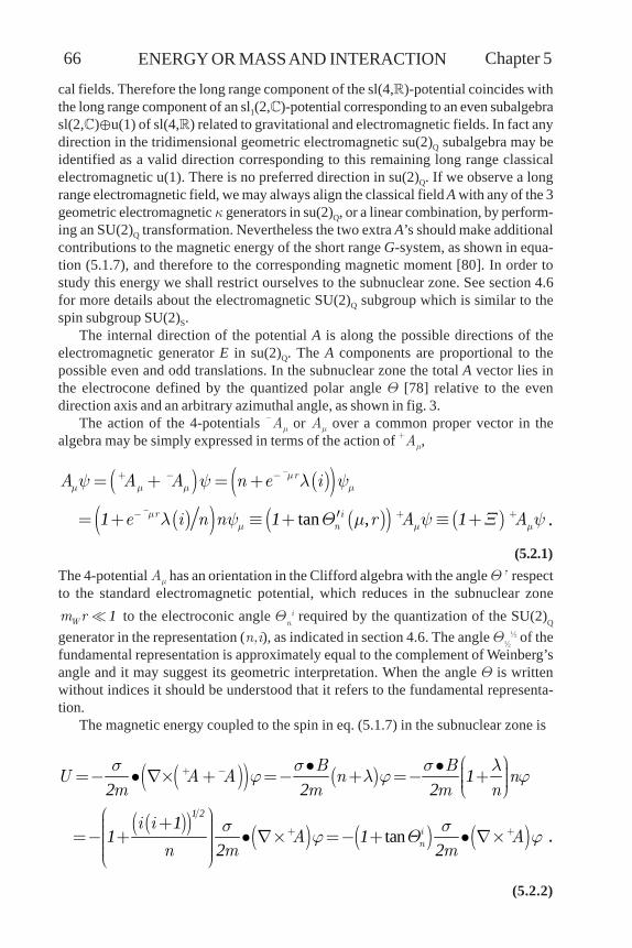
Chapter 5 ENERGY OR MASS AND INTERACTION66
cal fields. Therefore the long range component of the sl(4,)-potential coincides withthe long range component of an sl1(2,)-potential corresponding to an even subalgebrasl(2,)u(1) of sl(4,) related to gravitational and electromagnetic fields. In fact anydirection in the tridimensional geometric electromagnetic su(2)Q subalgebra may beidentified as a valid direction corresponding to this remaining long range classicalelectromagnetic u(1). There is no preferred direction in su(2)Q. If we observe a longrange electromagnetic field, we may always align the classical field A with any of the 3geometric electromagnetic k generators in su(2)Q, or a linear combination, by perform-ing an SU(2)Q transformation. Nevertheless the two extra A’s should make additionalcontributions to the magnetic energy of the short range G-system, as shown in equa-tion (5.1.7), and therefore to the corresponding magnetic moment [80]. In order tostudy this energy we shall restrict ourselves to the subnuclear zone. See section 4.6for more details about the electromagnetic SU(2)Q subgroup which is similar to thespin subgroup SU(2)S.
The internal direction of the potential A is along the possible directions of theelectromagnetic generator E in su(2)Q. The A components are proportional to thepossible even and odd translations. In the subnuclear zone the total A vector lies inthe electrocone defined by the quantized polar angle Q [78] relative to the evendirection axis and an arbitrary azimuthal angle, as shown in fig. 3.
The action of the 4-potentials -Am or Am over a common proper vector in thealgebra may be simply expressed in terms of the action of +Am,
( ) ( )( )( )( ) ( )( ) ( ) tan ,
r
r in
A A A n e i
e i n n r A A
mm m m m
mm m m
y y l y
l y Q m y X y
-
-
+ - -
- + +
= + = +
¢= + º + º +1 1 1 .
(5.2.1)The 4-potential Am has an orientation in the Clifford algebra with the angle Q’ respectto the standard electromagnetic potential, which reduces in the subnuclear zone
Wm r 1 to the electroconic angle Qni required by the quantization of the SU(2)Q
generator in the representation (n,i), as indicated in section 4.6. The angle Q½
½ of thefundamental representation is approximately equal to the complement of Weinberg’sangle and it may suggest its geometric interpretation. When the angle Q is writtenwithout indices it should be understood that it refers to the fundamental representa-tion.
The magnetic energy coupled to the spin in eq. (5.1.7) in the subnuclear zone is
( )( ) ( )
( )( ) ( ) ( ) ( ) tan1 2
12 2 2
11 1
2 2in
B BU A A n n
m m m n
i iA A
n m m
s s s lj l j j
s sj Q j
+ -
+ +
æ ö· · ÷ç=- · ´ + =- + =- + ÷ç ÷çè ø
æ ö+ ÷ç ÷ç ÷=- + · ´ =- + · ´ç ÷ç ÷ç ÷è ø .
(5.2.2)
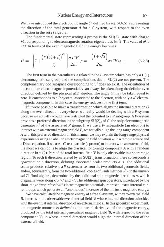
67Nuclear Energy and Interactions
We have introduced the electroconic angle Q, defined by eq. (4.6.5), representingthe direction of the total generator A for a G-system, with respect to the evendirection in the su(2) algebra.
The fundamental state representing a proton is the SU(2)Q state with charge+1, corresponding to electromagnetic rotation eigenvalues ½, ½. The value of Q isp/3. In terms of the even magnetic field the energy becomes
( )( ) ( )BU B
m ms
j s j+
+æ ö ++ ÷ç ÷ç ÷= - + = -ç ÷ç ÷ç ÷çè ø
1 21 1
2 2
12
1 311
2 2 . (5.2.3)
The first term in the parenthesis is related to the P-system which has only a U(1)electromagnetic subgroup and the complications due to SU(2) are not present. Thecomplementary odd subspace corresponding to S2 does no exist. The orientation ofthe complete electromagnetic potential A can always be taken along the definite evendirection defined by the physical u(1) algebra. The angle Q may be taken equal tozero. It corresponds to a P-system, associated to the electron, with only a k0 electro-magnetic component. In this case the energy reduces to the first term.
If it were possible to make a transformation which aligns the internal direction Qalong the even direction everywhere, we really would be dealing with a P-systembecause we actually would have restricted the potential to a P subgroup. A P-systemprovides a preferred direction in the subgroup SU(2)Q of G, the only electromagneticgenerator k0 of the associated P group. If we use a P-test-particle (an electron) tointeract with an external magnetic field B, we actually align the long range componentA with this preferred direction. In this manner we may explain the long-range physicalexperiments using an abelian electromagnetic field equation with a remote source anda Dirac equation. If we use a G-test-particle (a proton) to interact with an external field,the most we can do is to align the classical long-range component A with a randomdirection in su(2). Part of the total internal field iB is only observable in a short rangeregion. To each B direction related by an SU(2)Q transformation, there corresponds a“partner” spin direction, defining associated scalar products s.B. The additionalscalar products, relative to a P-system, arise from the two additional geometric fields,and/or, equivalently, from the two additional copies of Pauli matrices knk in the univer-sal Clifford algebra, determined by the additional spin-magnetic directions k, whichoriginally were along k1k2k3 and k5. The additional spin operators, introduced by theshort-range “non-classical” electromagnetic potentials, represent extra internal cur-rent loops which generate an “anomalous” increase of the intrinsic magnetic energy.
We have calculated the magnetic energy of a free G-system, with zero external fieldB, in terms of the observable even internal field +B whose internal direction coincideswith the eventual internal direction of an external field B. In this gedenken experiment,the magnetic moment is defined as the partial derivative of the magnetic energy,produced by the total internal generalized magnetic field iB, with respect to the evencomponent +B, in whose internal direction would align the internal direction of theexternal B field,
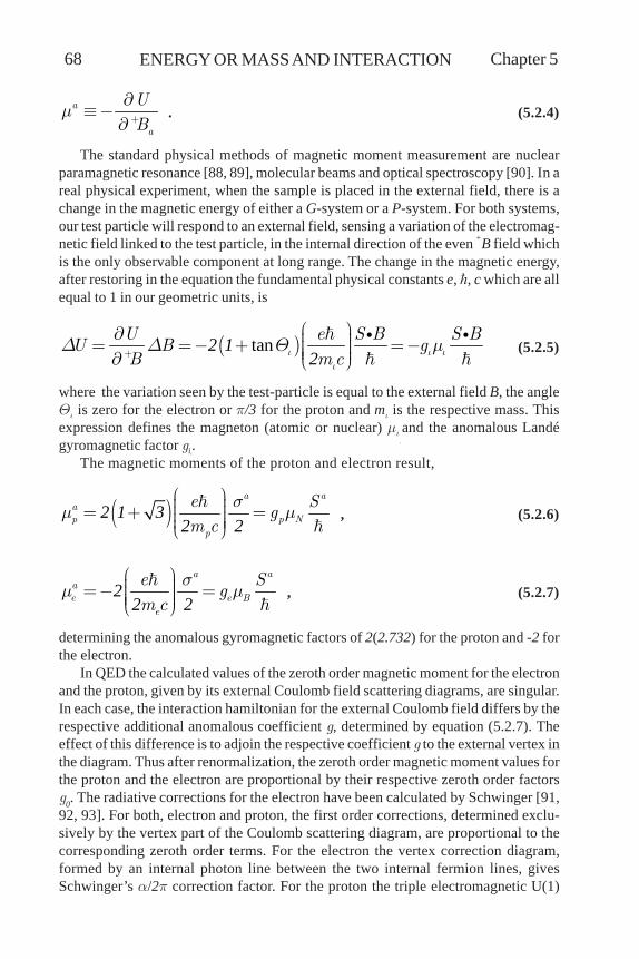
Chapter 5 ENERGY OR MASS AND INTERACTION68
a
a
UB
m +
¶º -
¶ . (5.2.4)
The standard physical methods of magnetic moment measurement are nuclearparamagnetic resonance [88, 89], molecular beams and optical spectroscopy [90]. In areal physical experiment, when the sample is placed in the external field, there is achange in the magnetic energy of either a G-system or a P-system. For both systems,our test particle will respond to an external field, sensing a variation of the electromag-netic field linked to the test particle, in the internal direction of the even +B field whichis the only observable component at long range. The change in the magnetic energy,after restoring in the equation the fundamental physical constants e, , c which are allequal to 1 in our geometric units, is
( )tanU e S B S BU B g
B m ci i ii
D D Q m+
æ ö¶ ÷ç ÷= = - + = -ç ÷ç ÷ç¶ è ø2 1
2
(5.2.5)
where the variation seen by the test-particle is equal to the external field B, the angleQi is zero for the electron or p/3 for the proton and mi is the respective mass. Thisexpression defines the magneton (atomic or nuclear) mi
i
and the anomalous Landé
gyromagnetic factor gii.
The magnetic moments of the proton and electron result,
( )a a
ap p N
p
e Sg
m cs
m mæ ö÷ç ÷ç= + =÷ç ÷÷çè ø
2 1 32 2
, (5.2.6)
a aae e B
e
e Sg
m cs
m mæ ö÷ç ÷= - =ç ÷ç ÷çè ø
22 2
, (5.2.7)
determining the anomalous gyromagnetic factors of 2(2.732) for the proton and -2 forthe electron.
In QED the calculated values of the zeroth order magnetic moment for the electronand the proton, given by its external Coulomb field scattering diagrams, are singular.In each case, the interaction hamiltonian for the external Coulomb field differs by therespective additional anomalous coefficient g, determined by equation (5.2.7). Theeffect of this difference is to adjoin the respective coefficient g to the external vertex inthe diagram. Thus after renormalization, the zeroth order magnetic moment values forthe proton and the electron are proportional by their respective zeroth order factorsg0. The radiative corrections for the electron have been calculated by Schwinger [91,92, 93]. For both, electron and proton, the first order corrections, determined exclu-sively by the vertex part of the Coulomb scattering diagram, are proportional to thecorresponding zeroth order terms. For the electron the vertex correction diagram,formed by an internal photon line between the two internal fermion lines, givesSchwinger’s a/2p correction factor. For the proton the triple electromagnetic U(1)

69Nuclear Energy and Interactions
structure present in the SU(2) sector of the geometric interaction operator JG, deter-mines three standard j.A coupling terms. The triple structure is also present in thenoncompact sector of the algebra. This indicates that a full proton excitation descrip-tion requires three boost momenta ki. Consequently a full description of the externalCoulomb field scattering diagram requires a pair of internal fermion boost momentumtriplets, instead of simply the pair of electron momenta. There are additional U(1)radiative processes between the six internal fermion boost lines corresponding to thetwo triplets. Therefore, there are multiple additional internal vertex diagrams, obtainedby permutation of the internal photon line among the six necessary internal fermionlines, which contribute to the first order correction. The multiplicity of the vertexcorrections of the 6 lines taken 2 at a time is 15. Each correction is equal to Schwinger’svalue, a/2p, due the SU(2)
Q group equivalence. Up to first order, the proton mag-
netic moment is
. ( . ) .gg ap
æ ö÷ç= + = + =÷ç ÷çè ø01 151 2 7321 1 0 01742 2 7796
2 2 2 . (5.2.8)
Let us calculate the magnetic moment of a combination of GPL chain excita-tions. The total electromagnetic potential is the sum of the SU(2)Q A potential anda different U(1) AU potential. Let j be a (½) eigenfunction of A and AU [63]. Includ-ing the radiative correction, with the 28 vertex multiplicity corresponding to 4 P-excitations in the resultant su(2)+u(1) algebra, the magnetic moment of the combi-nation is
( )
( ) . .
a aa
n Np
a
N
e Sg
m c
S
a sm m
p
m
æ öæ ö ÷ç÷ç ÷ç= - + + =÷ ÷ç ç÷ç ÷è ø ÷çè ø
= -
282 1 3 2 12 2 2
2 1 967
(5.2.9)
These results have a 0.5% discrepancy with the experimental values of theproton magnetic moment (2.7928) and the neutron magnetic moment (1.9130).The neutron may be considered a combination of the proton, the electron and theantineutrino.
5.3. The Modified Pauli Equation.If the generalized Pauli equation (5.1.7) in the subnuclear zone is useful in
calculating the magnetic moments of the nucleons we may expect that this equa-tion is involved in the nuclear interaction. In particular we are interested in apply-ing it to the study the properties of the light stable nuclides [94]. A nonlinearsubstratum solution implies the self interaction between its excitation field andmotion. It is normal to define the self potential of a charge as positive. With theadequate definition of the classic potential A, in accordance with section 3.6, andusing eqs. (5.2.1) and (5.1.7) for the quantum states of the potential A we obtain,
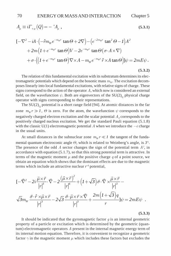
Chapter 5 ENERGY OR MASS AND INTERACTION70
( )A i Q Am m mG ++º = - , (5.3.1)
( ) ( )( ) ( )
( )( )
ˆ[ tan tan
tan tan
ˆ tan tan ]
W W
W W
W W
m r m rW
m r m r
m r m rW
iA rm e e A
m e V e A
e A m e r A mE
Q Q
Q Q s
s Q Q y y
- -
- -
- -
- - ⋅ - + - -
+ + - ⋅ ´
+ ⋅ + ´ - ´ =
22 2 22 1
2 1 2
1 2 .
(5.3.2)The relation of this fundamental excitation with its substratum determines its elec-
tromagnetic potentials which depend on the bosonic mass mW. The excitation decom-poses linearly into local fundamental excitations, with relative signs of charge. Thesesigns correspond to the action of the operator A, which now is considered an externalfield, on the wavefunction y. Both are eigenvectors of the SU(2)Q physical chargeoperator with signs corresponding to their representations.
The SU(2)Q potential is a short range field [94]. At atomic distances in the farzone Wm r 1 , Q is zero. For the atom, the wavefunction y corresponds to thenegatively charged electron excitation and the scalar potential A0 corresponds to thepositively charged nucleus excitation. We get the standard Pauli equation (5.1.8)with the classic U(1) electromagnetic potential A when we introduce the -e chargein the usual units.
At small distances in the subnuclear zone Wm r 1 the tangent of the funda-mental quantum electroconic angle Q, which is related to Weinberg’s angle, is 3½.The presence of the odd A sector changes the sign of the potential term A2, inaccordance with equation (5.1.7), so that this strong potential term is attractive. Interms of the magnetic moment m and the positive charge q of a point source, weobtain an equation which shows that the dominant effects are due to the magneticterms which include an attractive nuclear r-4 potential,
( ) ( )
( )
[
ˆ]W
rr ri
r r r
m qr r rm mE
rr r
mm ms
s m s my y
´´ ´- - ⋅ - + + ⋅ ´ -
+⋅ ´ ´ ⋅ ´ ´- + =
22
3 6 3
3 3
2 2 1 3
2 1 33 2 3 2
.
(5.3.3)It should be indicated that the gyromagnetic factor g is an internal geometric
property of a particle or excitation which is determined by the geometric (quan-tum) electromagnetic operators A present in the internal magnetic energy term ofits internal motion equation. Therefore, it is convenient to recognize a geometricfactor g in the magnetic moment m which includes these factors but excludes the

71Nuclear Energy and Interactions
mass which represents a secondary inertial reaction in the charge motion. De-pending on the particular system considered this mass may correspond to thesystem reduced mass or to a total mass.
5.4. The Proton-Electron-ProtonModel for the Deuteron.
Consider that equation (5.3.3) represents a system of G and P excitations, in par-ticular a system of one electron and two protons moving about the system center ofmass. The fields are dominated by the electron magnetic field because its highermagnetic moment m. The resultant SU(2) field is characterized by the system reducedmass which is the electron mass m. There are flux quanta associated to the protons pand the electron e, one for each particle, which should link among themselves. Thismakes convenient to use the flux lines or magnetic strings to characterize the linksbetween particle magnetic moments. The dominant potential is a strong attraction inthe equatorial radial direction which may also be considered as the attraction amongmagnetic flux lines linked to flux quanta. The three indicated quantum flux stringscannot be linked so that they fully attract themselves as a whole without breaking thePauli exclusion principle of the two p. To fully attract themselves the only possibility isthe necessary presence of a fourth string. This string must be supplied by the onlyneutral fundamental excitation in the theory, an L excitation or neutrino with a linked
flux quantum. The resultant system ( ), , ,p e pn is a model for the deuteron. The only
possible way to attractively link the flux lines determines that the subsystem ( ),e en ¢º
has the e and spins in the same direction. Hence e’ has spin 1, the charge, mass andthe magnetic moment of the electron. The operators +Ae of the electron e and Ap of the
protons p in the stable system ( ), ,p e p¢ constitute a single coherent total field operator A,which depends on the reduced mass, and determines its fundamental SU(2) excitation.In other words, the resultant 4-potencial A has the Clifford algebra orientation re-quired by the fundamental SU(2)Q quantum representation of the generator. This de-termines the geometric electroconic angle Q of A with respect to the even electromag-netic potential +A. The resultant field affects the system components and in particularthe protons. The dominant internal magnetostatic energy is the one which holds the
excitation system ( ), ,p e p¢ together and determines its energy proper value E. Wemay say that this is a coherent symmetric quasi-static disposition of the two pro-tons around the excited electron in a proton-electron-proton formation which fa-cilitates a stable solution.
Because of the symmetry we may use cylindrical coordinates with the z axisalong the electron magnetic moment m. It is convenient to approximate the poten-tials to very small r by only keeping the dominant r-4 potential term. The energy
eigenvalue is expressed as a mass fraction E me= 2 . In this manner we obtain [94]the equation

Chapter 5 ENERGY OR MASS AND INTERACTION72
mz
me y
rr
é ùê úê úê ú- - - =ê úæ öê ú÷ç ÷+ê úç ÷ç ÷çê úè øë û
22 2 2
324
2
22 01
. (5.4.1)
This equation is not separable [95] due to the spatial polar angle q dependencecontained in the cross products.
Nevertheless, since orbital and spin angular momenta tend to align with themagnetic B field we should expect that the wave function concentrates around theequatorial plane and most of the energy is in the equatorial region. A calculationof the negative gradient of the dominant potential term confirms this consider-ation. The negative gradient has direction toward the equatorial plane z = 0 for allvalues of z and toward the origin in an equatorial region defined by z r<2 22 . Thisequatorial region is limited by two cones near the equator, characterized by an equa-torial angle or latitude qe . In the limit of very small r the problem reduces to abidimensional problem on the equatorial plane. Therefore, near this limit we shouldsimplify by setting sin q » 1 , z » 0 ., obtaining a separable approximate equation,
mm
e yr
é ùê ú + + =ê úë û
22 2 2
4
22 0 , (5.4.2)
mz
me y
r r r r j r
é ù¶ ¶ ¶ ¶ê ú+ + + + + =ê ú¶ ¶ ¶ ¶ë û
2 2 2 22 2
2 2 2 2 4
1 1 22 0 . (5.4.3)
Since the z dependence is originally through the spatial polar angle q, it is conve-nient to introduce in its place, in the equatorial zone, an angular latitude coordinate z,.In terms of this coordinate in the equatorial region the equation becomes
mm
r r e r yr r j z r
é ù¶ ¶ ¶ ¶ê ú+ + + + + =ê ú¶ ¶ ¶ ¶ë û
2 2 2 22 2 2 2
2 2 2 2
22 0 . (5.4.4)
We assume a separable solution in the equatorial region, of the form
( ) ( ) ( )R Zy r L j z= . (5.4.5)
The separated equation for Z , which does not produce eigenvalues, is
ZZa
z¶
=¶
22
2 (5.4.6)
where a is only an approximate separation constant.
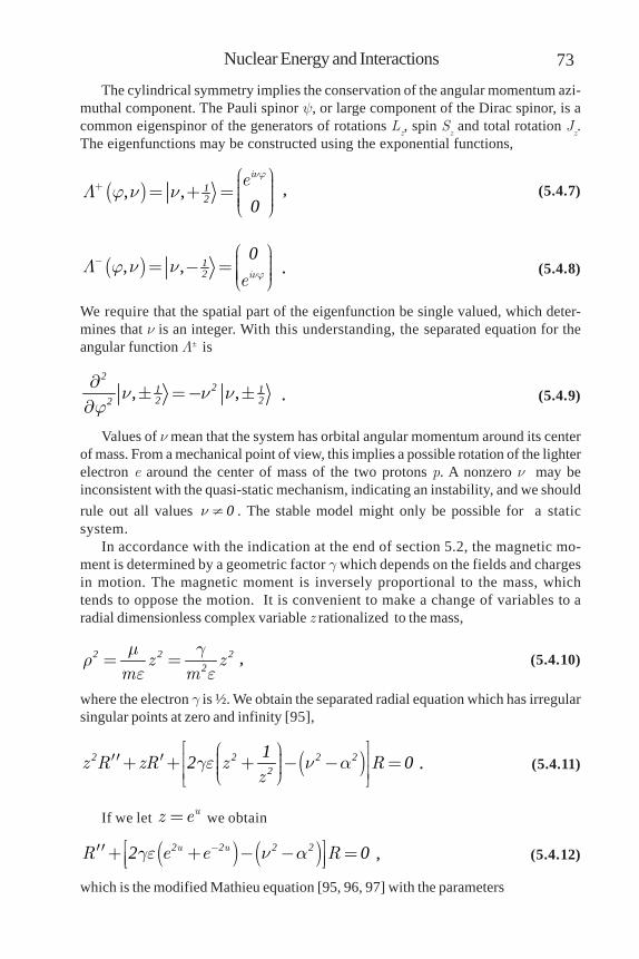
73Nuclear Energy and Interactions
The cylindrical symmetry implies the conservation of the angular momentum azi-muthal component. The Pauli spinor y, or large component of the Dirac spinor, is acommon eigenspinor of the generators of rotations L
z, spin S
z and total rotation J
z.
The eigenfunctions may be constructed using the exponential functions,
( ), ,ie nj
L j n n+æ ö÷ç ÷= + = ç ÷ç ÷çè ø
12 0
, (5.4.7)
( ), , ie njL j n n-æ ö÷ç= - = ÷ç ÷ç ÷çè ø
12
0 . (5.4.8)
We require that the spatial part of the eigenfunction be single valued, which deter-mines that n is an integer. With this understanding, the separated equation for theangular function L± is
, ,n n nj
¶ = -
¶
221 1
2 22 . (5.4.9)
Values of n mean that the system has orbital angular momentum around its centerof mass. From a mechanical point of view, this implies a possible rotation of the lighterelectron e around the center of mass of the two protons p. A nonzero n may beinconsistent with the quasi-static mechanism, indicating an instability, and we shouldrule out all values n ¹ 0 . The stable model might only be possible for a staticsystem.
In accordance with the indication at the end of section 5.2, the magnetic mo-ment is determined by a geometric factor g which depends on the fields and chargesin motion. The magnetic moment is inversely proportional to the mass, whichtends to oppose the motion. It is convenient to make a change of variables to aradial dimensionless complex variable z rationalized to the mass,
z zm mm g
re e
= =2 2 22 , (5.4.10)
where the electron g is ½. We obtain the separated radial equation which has irregularsingular points at zero and infinity [95],
( )z R zR z Rz
ge n aé ùæ ö÷çê ú¢¢ ¢+ + + - - =÷ç ÷çê úè øë û
2 2 2 22
12 0 . (5.4.11)
If we let uz e= we obtain
( ) ( )u uR e e Rge n a-é ù¢¢ + + - - =ê úë û2 2 2 22 0 , (5.4.12)
which is the modified Mathieu equation [95, 96, 97] with the parameters

Chapter 5 ENERGY OR MASS AND INTERACTION74
q ge= 2 , (5.4.13)
a n a= -2 2 . (5.4.14)In the last equation the parameters a, and a should be considered effective param-eters because, independently of n2 and a2, a may include contributions from equation(5.4.1). Nevertheless, the eigenvalues of the angular and radial equations are the oneswhich directly determine the possible values of the pair n, a and consquently theeffective value a2.
This approximate result regarding the application of the Mathieu equation forthe system under study might also be obtained using spherical coordinates.
5.5. Binding Energy of the Deuteron.According to Floquet’s theorem [84], a solution of eq. (5.4.12) includes an
overall factor, sue where s is a complex constant. If s is an integer we get the Mathieufunctions of order s. A Mathieu function [95] is one of the few special functionswhich are not a special case of the hypergeometric function and therefore thedetermination of its proper values differs. The Mathieu functions can be expressedas a Fourier series. The series expansion coefficients are proportional to the char-acteristic root values ar of a set of continued fraction equations obtained from thethree-term recursion relations among the expansion coefficients. These character-istic roots are obtained as a power series in q.
A solution of the Mathieu equation can also be expressed in terms of a seriesof Bessel functions with the same expansion coefficients of the Fourier series.This Bessel series is convenient to find the asymptotic behavior of the solution.By replacing the Bessel functions with the Neumann functions we obtain a solu-tion of the second kind. Solutions of the third and fourth kind are obtained bycombining the Bessel and Neumann functions to form Hankel functions. We wanta regular solution at zero that vanishes at infinity. We require that s = 0 to avoid asingular or oscillatory asymptotic behaviour. The appropriate negative exponentialbehavior at infinity is provided by the radial Mathieu function of zeroth order, of the
third kind, or Mathieu-Hankel function, indicated by ( ),He q u0 .It is known that the characteristic roots and the corresponding series expan-
sion coefficients for the Mathieu functions have branch cut singularities on theimaginary q axis[98, 99] and the complex plane a of the corresponding Riemannsurfaces. Therefore, the expansion coefficients are multiple-valued. In the stan-dard radial equation eigenvalue problem, the energy is determined by eliminating thesingularities of the hypergeometric series by requiring its coefficients to vanish aftera certain order. In our case, the energy should be determined by eliminating the branchcut singularity of the Mathieu series by choosing appropriate coefficients. We shouldrequire that the solution coefficients of the R function be single valued as werequired for the L function. To eliminate the possibility of multiple-valued coeffi-cients and obtain a regular solution we must disregard all points q on all branches ofthe Riemann surface except the points q0 common to all branches. We require that q be
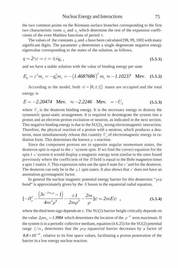
75Nuclear Energy and Interactions
the two common points on the Riemann surface branches corresponding to the firsttwo characteristic roots a
0 and a
2 which determine the rest of the expansion coeffi-
cients of the even Mathieu functions of period p.The values of the constants q0 and a have been calculated [98, 99, 100] with many
significant digits. The parameter q determines a single degenerate negative energyeigenvalue corresponding to the states of the solution, as follows,
q iqge e= = = 02 , (5.5.1)
and we have a stable solution with the value of binding energy per state
( ). . Mev.e e eE m q m me= = - = - » -22 2
0 0 1 4687686 1 10237 (5.5.2)
According to the model, both ,y = 120 states are occupied and the total
energy is
. Mev. . Mev. dE U= - » - = -2 20474 2 2246 (5.5.3)
where Ud is the deuteron binding energy. It is the necessary energy to destroy the
symmetric quasi-static arrangement. It is required to desintegrate the system into aproton and an electron-proton excitation or neutron, as indicated in the next section.This negative binding energy is due to the SU(2)Q strong electromagnetic interaction.Therefore, the physical reaction of a proton with a neutron, which produces a deu-teron, must simultaneously release this cuantity U
d of electromagnetic energy in ra-
diation form. This determines the known p n reaction.Since the component protons are in opposite angular momentum states, the
deuteron spin is equal to the e’ system spin. If we find the correct equation for thespin 1 e’ system it would display a magnetic energy term similar to the ones foundpreviously where the coefficient of the B field is equal to the Bohr magneton timesa spin 1 matrix S. This expression rules out the spin 0 state for e’ and for the deuteron.The deuteron can only be in the ±1 spin states. It also shows that e’ does not have ananomalous gyromagnetic factor.
In general the nuclear magnetic potential energy barrier for this deuteronic “pepbond” is approximately given by the A boson in the equatorial radial equation,
( )[ ]
Ame mmE
m m
r
r y yr r r
--
-¶ - - - =2
22 4 3
3 1 1 2 24 2
, (5.5.4)
where the third term sign depends on y. The SU(2) barrier height critically depends on
the value .Amr =2 1 3984 which determines the location of the r-4 term maximum. Ifthe system is in a periodic collective medium, equation (4.6.25) for the SU(2) potentialrange 1/mA determines that the pep equatorial barrier decreases by a factor of
. -´ 148 8 10 , relative to its free space values, facilitating a proton penetration of thebarrier in a low energy nuclear reaction.
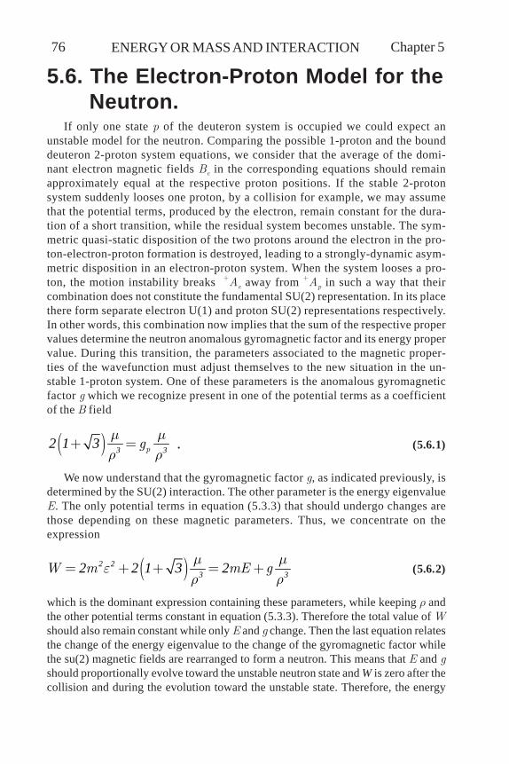
Chapter 5 ENERGY OR MASS AND INTERACTION76
5.6. The Electron-Proton Model for theNeutron.
If only one state p of the deuteron system is occupied we could expect anunstable model for the neutron. Comparing the possible 1-proton and the bounddeuteron 2-proton system equations, we consider that the average of the domi-nant electron magnetic fields Be in the corresponding equations should remainapproximately equal at the respective proton positions. If the stable 2-protonsystem suddenly looses one proton, by a collision for example, we may assumethat the potential terms, produced by the electron, remain constant for the dura-tion of a short transition, while the residual system becomes unstable. The sym-metric quasi-static disposition of the two protons around the electron in the pro-ton-electron-proton formation is destroyed, leading to a strongly-dynamic asym-metric disposition in an electron-proton system. When the system looses a pro-ton, the motion instability breaks +Ae away from +Ap in such a way that theircombination does not constitute the fundamental SU(2) representation. In its placethere form separate electron U(1) and proton SU(2) representations respectively.In other words, this combination now implies that the sum of the respective propervalues determine the neutron anomalous gyromagnetic factor and its energy propervalue. During this transition, the parameters associated to the magnetic proper-ties of the wavefunction must adjust themselves to the new situation in the un-stable 1-proton system. One of these parameters is the anomalous gyromagneticfactor g which we recognize present in one of the potential terms as a coefficientof the B field
( ) pgm mr r
+ =3 32 1 3 . (5.6.1)
We now understand that the gyromagnetic factor g, as indicated previously, isdetermined by the SU(2) interaction. The other parameter is the energy eigenvalueE. The only potential terms in equation (5.3.3) that should undergo changes arethose depending on these magnetic parameters. Thus, we concentrate on theexpression
( )W m mE gm m
er r
= + + = +2 23 32 2 1 3 2 (5.6.2)
which is the dominant expression containing these parameters, while keeping r andthe other potential terms constant in equation (5.3.3). Therefore the total value of Wshould also remain constant while only E and g change. Then the last equation relatesthe change of the energy eigenvalue to the change of the gyromagnetic factor whilethe su(2) magnetic fields are rearranged to form a neutron. This means that E and gshould proportionally evolve toward the unstable neutron state and W is zero after thecollision and during the evolution toward the unstable state. Therefore, the energy

77Nuclear Energy and Interactions
eigenvalue is proportional to the gyromagnetic factor and to the intrinsic magneticmoment potential term which is a fraction of total effective potential
n
n p
EEEg g g
= = 0 . (5.6.3)
The ratio of the two nucleon energy eigenvalues is then approximately equal to theratio of the gyromagnetic factors. We know from section 5.2 that both anomalousproton and neutron magnetic moments are determined and theoretically calculatedfrom two different su(2) magnetic field arrangements in nucleon excitation systemswith mass mp. The proton-electron system undergoes su(2) magnetic field changestoward an unstable neutron system which eventually decays. The energy of the lattersystem is then theoretically determined by these gyromagnetic factor theoretical val-ues
( ). . . Mev. . Mev..n n p eE m m m
-= - = » - - =
1 967 1 10237 0 780 0 7822 780
(5.6.4)This system has a mass-excess equal to En which is given-up as energy when itdecays into its constituents proton and electron.
The generalized Pauli equation (5.3.3) for the internal motion relative to thecenter of mass, with reduced mass m, under the internal magnetic field, serves tocalculate gyromagnetic effects and binding energies. The Pauli equation also servesto study the motion of the neutron system center of mass under an external magneticfield, now with the resultant total mass.
The system ( ), ,p e n is a spin ½ system because the proton spin is opposite to
the ( ),e en ¢º spin. Thus, the neutron and proton forming the deuteron have theirspins in the same direction. The fact that the deuteron magnetic moment is theapproximate sum of the proton and neutron moments may be explained becausethe presence of an external magnetic field forces one proton to react by itself whilethe rest of the system, p, e’ reacts adjusting its fields as a neutron.
5.7. The Many Deuteron Model.We follow here the idea of nuclear pairings by Bohr, Mottelson and Rainwater
[101]. The presence of orbital angular momentum, l ¹ 0 , breaks the stable quasi-static mechanism of the model. The equation determines only one stable bondexcitation corresponding to the spin ±½ states of frame field excitations bound by thestrong magnetic interaction. This deuteron “pep bond” is a (p,e’,p) fundamentalexcitation and supplies another pairing mechanism which also allows the combi-nation of more than 2 protons. The alpha particle, or excitation a, may be consid-ered as a 2-deuteron excitation [102].
The magnetic interaction range defines the subnuclear zone W pr m r1 ,

Chapter 5 ENERGY OR MASS AND INTERACTION78
very small in relation to the proton radius rp. Mathieu’s equation determines a singlepep bond energy in a proton pair. In order to feel the strong attraction the protoncenters must be inside the subnuclear zone. Therefore the protons are essentiallysuperposed. In the a model there are 4 protons and 2 electrons which are also super-posed and must share the magnetic field. The stationary state, of minimum energy,is the symmetrized quantum superposition, as in the hydrogen molecular ion. Theelectrons and protons are shared by all possible pep bonds in the system. The pos-sible pep bonds obey the Pauli exclusion principle and are only those sharing a singleelectron. All p participate in as many pep bonds as proton pairings.
One difference in the a model is that the reduced mass m of the system isapproximately half the electron mass me due to the presence of two electrons inthe system. The required coordinate transformation to obtain Mathieu’s equationis then different from eq. (5.4.10),
e
z z zm m m mm g g
re e e
= = =2 2 2 222
, (5.7.1)
which changes q proportionally and determines twice the binding energy dU ¢ perpair,
q e= 2 , (5.7.2)
( )d e dE E m q m q m Ue¢ ¢= = = =- =-22 20 02 2 2 2 4 2 . (5.7.3)
The energy d dE E¢ = 2 is the unique Mathieu equation eigenvalue even if e' isshared and is the same for each pep magnetic bond. This fact together with thesymmetry simplifies the energy calculation of the n-body problem. There are symmet-ric cluster states whose energies are determined by their pep bonds. The symmetric acluster associated to 4 protons has 6 pep bonds and the energy of these bonds minusthe electronic mass difference,
, ,
, ,
p e p e
i i ep e p em m m
¢ ¢
¢¢ ¢= -å å4 2 4 6 4 , (5.7.4)
( ) ,, . Mev.e d ep ep eE E m E m E Ua a¢¢
¢= - = - = - º » -4 64 2 4 6 4 28 501 .
(5.7.5)Similarly we have the same considerations for 3 protons.The symmetric cluster
associated to 3 protons has 3 pep bonds with a unique Mathieu energy Ed,
( ) ,, . Mev. He Hee d ep ep eE E m E m E U¢¢ = - = - = - º » -3 33 33 2 3 2 7 636 .
(5.7.6)The exclusion principle prohibits 2e in a pep bond. An extra e may link to a p which is notin pep bond at that moment, which is impossible in the 4p a system, with the energy of eq.(5.6.4),

79Nuclear Energy and Interactions
( )e n pE m m mD = - - , (5.7.7)
( ), . Mev.He H Hp eE E E E U¢ = + D = - º » -3 3 33 2 8 416 . (5.7.8)
These equations determine a mass relation identity for the A=3 isobars. Since
our notation uses the correspondence ( ) ( ), ,p e p n¢ =3 2 we may write
p n p n eH He He
eH He
m m m E E m m m E
m m m
+
+ +
= + + + D = + + +
º +
3 3 3
3 3 2
2 2(5.7.9)
which indicates a small b decay possibility of 3H+ into 3He+ from total energyconsiderations in spite of the unfavorable binding energy difference. It also im-plies that the corresponding atoms 3He and 3H have essentially equal masses, upto the negligible Coulomb electron interaction.
5.7.1. Nuclear Structure, Fusion and Fission.We have obtained the binding energies for 4He and the isobars 3H, 3He within
1%. We are lead by the model to consider that the pep bonds or deuterons act as theessential components of more complex clusters in electromagnetic interaction withadditional nucleons. This is consistent with the protonic and neutronic numbersof the nuclides. Any proton outside a pep bond when associated with e' may beconsidered a neutron. Therefore the energy bond Ud determines a “nuclear” force ofelectromagnetic origen among nucleons, which is independent of a neutron inter-pretation. These simple facts about deuterons and alpha particles would deter-mine the general nuclear structure. The inclusion of neglected interaction terms maybe sufficient, without any other force, to explain the properties of nuclides and theirfusion and fission reactions.
We have built these models using the geometric ideas, in particular the electro-magnetic SU(2)Q subgroup and its attractive subnuclear r-4 potential term. It shouldbe clear that the numbers obtained also depend on other particular model features andthey do not constitute by themselves a proof of the theory. Nevertheless the overallpicture lends them credibility. From a practical point of view these results should notbe overlooked because the implications they might have in the understanding of theprocess of nuclear fusion of light nuclei. The electromagnetic field would be anactive element of a fusion generator. In particular it may provide possible quasistatic fusion processes for the development of clean fusion energy without the presentproblems of high radiation and radioactivity.
The binding energy of the deuteron and other light nuclides would be essen-tially magnetostatic and the nuclear fission and fusion reactions in a nuclidesystem would be magnetic multipolar transitions. The electromagnetic field mayinterchange electromagnetic gamma radiation of type M1 through the correspond-ing quantum or gamma photon. If the system interacts with another (external)system, in addition to the radiative channel there should be other possible chan-

Chapter 5 ENERGY OR MASS AND INTERACTION80
nels in the S dispersion matrix. The total potential may have energy transfers inthe non radiation near zone. Quasistatic channels may open between the nuclidesystem and the other system through the field in this electromagnetic zone. Inparticular, if the potential is periodic and coherent in a collective system thecuantum magnetic barrier for quasistatic exchanges may be reduced, as indicatedin section 5.5. In this manner magnetic energy would be tranferred with low radia-tion, as it usually happens between near electromagnetic and matter systems.
5.8. Geometric Weak Interations.In addition to the strong effects shown in the previous sections it is also
possible to find weak effects. The field equation implies a conservation law for thegeometric current, which determines a generalized Dirac equation (3.6.1) in termsof the local frames. This equation, for the even and odd parts of a frame f under thepresence of a pure odd potential reduces [7] as seen in chapter 3 to
f A f mfm mm mk ¶ k+ - - -= = , (5.8.1)
f A f mfm mm mk ¶ k- - + += = , (5.8.2)
implying that a frame for a massive corpuscle must have odd and even parts. Foran even frame,
=f m- = 0 0 . (5.8.3)
Therefore, for an even frame we obtain the equation normally associated with aneutrino field by multiplying by k0. A fluctuation of f+ on the fixed substratumobeys also the last equation.
From previous discussion, [103] we consider that an electroweak interactionmay be related to the action of the Sp(2,) holonomy group. The total interactionfield should correspond to a potential A, which is a representation of Sp(2,).The total matter current should be associated to an Sp(2,) frame f representingboth the electron field e and the neutrino field n. We should then be able todescribe neutrino electron interactions.
At a point, the total frame excitation f of the interacting e,n is related to anelement of the group Sp(2,), a subspace of the geometric algebra R3,1=R(4). Theframe f may be decomposed into fields associated to the particles e,n by means ofthe addition operation within the algebra. These e, n fields are not necessarilyframes because addition does not preserve the group subspace Sp(2,) andgeometrically, e and n are not sections of a principal fiber bundle but rather of anassociated bundle with the Clifford algebra as fiber.
The source current J in the theory is
J f f f fk k= = , (5.8.4)
where f is the frame section associated to the total field of the electron and theneutrino and k represents the orthonormal set. For the Sp(2,) group the correla-tion reduces to conjugation.
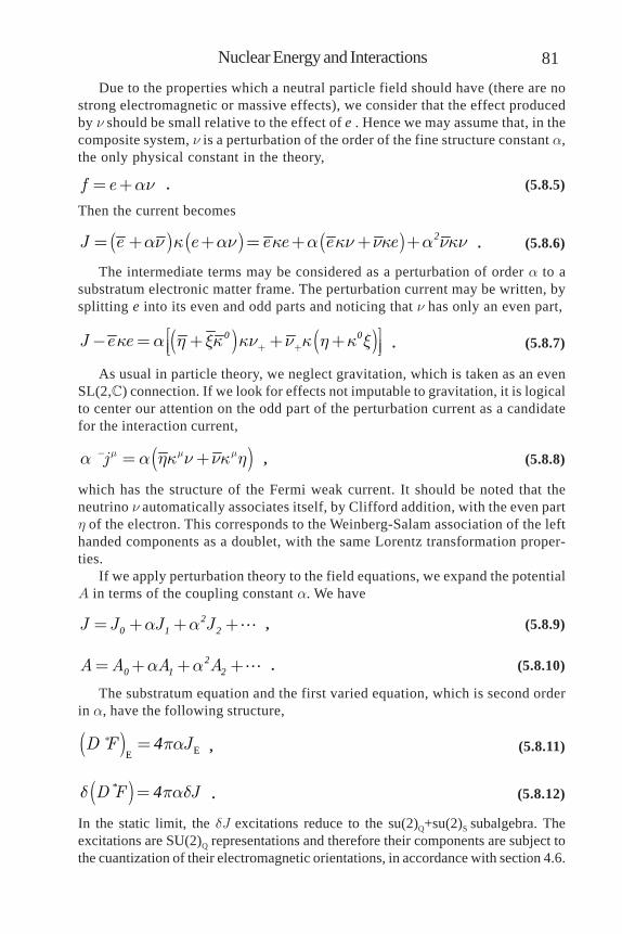
81Nuclear Energy and Interactions
Due to the properties which a neutral particle field should have (there are nostrong electromagnetic or massive effects), we consider that the effect producedby n should be small relative to the effect of e . Hence we may assume that, in thecomposite system, n is a perturbation of the order of the fine structure constant a,the only physical constant in the theory,
f e an= + . (5.8.5)
Then the current becomes
( ) ( ) ( )J e e e e e ean k an k a kn nk a nkn= + + = + + + 2 . (5.8.6)
The intermediate terms may be considered as a perturbation of order a to asubstratum electronic matter frame. The perturbation current may be written, bysplitting e into its even and odd parts and noticing that n has only an even part,
( ) ( )J e ek a h xk kn n k h k x+ +é ù- = + + +ê úë û
0 0 . (5.8.7)
As usual in particle theory, we neglect gravitation, which is taken as an evenSL(2,) connection. If we look for effects not imputable to gravitation, it is logicalto center our attention on the odd part of the perturbation current as a candidatefor the interaction current,
( )j m m ma a hk n nk h- = + , (5.8.8)
which has the structure of the Fermi weak current. It should be noted that theneutrino n automatically associates itself, by Clifford addition, with the even parth of the electron. This corresponds to the Weinberg-Salam association of the lefthanded components as a doublet, with the same Lorentz transformation proper-ties.
If we apply perturbation theory to the field equations, we expand the potentialA in terms of the coupling constant a. We have
J J J Ja a= + + +20 1 2 , (5.8.9)
A A A Aa a= + + +20 1 2 . (5.8.10)
The substratum equation and the first varied equation, which is second orderin a, have the following structure,
( ) EED F Jpa* = 4 , (5.8.11)
( )*D F Jd pad= 4 . (5.8.12)
In the static limit, the dJ excitations reduce to the su(2)Q+su(2)S subalgebra. Theexcitations are SU(2)Q representations and therefore their components are subject tothe cuantization of their electromagnetic orientations, in accordance with section 4.6.

Chapter 5 ENERGY OR MASS AND INTERACTION82
We should express the term J1 as a function of its odd component. In this manner, welet the first order terms be, as a function of the representation electrocone angle Q,
sinJ j j Q-= =1 , (5.8.13)
A W=1 , (5.8.14)
and we obtain for the variation, the linear equation
( )d dW LW ja pa* + = 24 , (5.8.15)
where L is a linear first order differential operator determined by the substratum.This equation may be solved in principle using its Green’s function . The solu-tion in terms of components with respect to a base E in the algebra is
( ) ( )ji i j
j xx xW dx nm mnpa ¢¢= ¢ -ò4 . (5.8.16)
It is well known that the second variation of a lagrangian serves as lagrangianfor the first varied Euler equations. Therefore, the AJ term in the covariant deriva-tive present in the lagrangian [8, 9] provides an interaction coupling term thatmay be taken as part of the lagrangian for the process in discussion. When the AJterm is taken in energy units, considering that the lagrangian has an overall mul-tiplier, it should lead to the interaction energy for the process. The second varia-tion (or differential) in a Taylor expansion of the energy U, corresponds to thehessian of U.
The AJ term gives the interaction lagrangian for the substratum, in energyunits. For the perturbations, the interaction lagrangian is given by 1/2 the secondvariation or dJ.dA,
( )tr W j j Wm mm ma- +2 1 1
4 2 = . (5.8.17)
It is clear that this interaction is carried by G or W. Nevertheless, we wish toobtain a current-current interaction to compare with other theories at low ener-gies. Substitution of eq. (5.8.16) in the last equation gives the correspondingaction which, for clarity, we indicate by
( ) ( ) ( )tr j i l l ii j lx x E E E E j x j xdxdx m nmnpa é ù¢ ¢¢ - += - ê úë ûò3 1
42 ,
(5.8.18)representing a current-current interaction hamiltonian, with a coupling constantderived from the fine structure constant. This new expression may be interpretedas a weak interaction Fermi lagrangian. The associated coupling constant is of thesame order as the standard weak interaction coupling constant, up to terms in theGreen’s functions .

83Nuclear Energy and Interactions
5.9. Relation with Fermi’s Theory.The action, in terms of elements of the algebra and the trace, corresponds to
the scalar product. For the case of the isotropic homogeneous constant substra-tum solution, eq. (1.3.2), the Greens function is a multiple of the unit matrix withrespect to the algebra components. We assume here that for a class of solutionsthe Green’s function have this property. Then for this class of solutions, the lastequation may be written as
( ) ( ) ( )tr x x j x jdxdx xm nmnpa ¢¢= - ¢-ò3 1
44 , (5.9.1)
where the j are matrices.The current defines an equivalent even current j- , which is the k0 component,
by inserting k0k0 and commuting. Each 2´2 block component of this 4 dimensional
real current matrix is an even matrix which may be represented as a complex num-ber, by the known isomorphism between this complex algebra and a subalgebra of2´2 matrices. Thus, we may use, instead of the generalized spinors forming theframe f, the standard bidimensional spinor pairs, h1, h2 and n1, n2 which form the2´2 submatrices corresponding to the even part, respectively, of the electron andthe neutrino. In this manner, if we use the standard quantum mechanics notationin Weyl’s representation, each matrix component is of the form
( ) †e nj m m mY g g Y h s n- = + =51 1
2 , (5.9.2)
which may be recognized as the standard nonhermitian Fermi weak interactioncurrent for the electron neutrino system. We shall indicate this current by jF andwe may determine that the 0-0 submatrix j0 is the hermitian part of jF.
We may evaluate the trace of the currents in the expression for . As dis-cussed previously, within this theory, particles would be represented by excita-tions of frames. These fluctuations are matrices which correspond to a singlerepresentation of the subgroup in question. This means that for each pair ofspinors of a spinor frame, only one is active for a particular fluctuation matrix. Inother words, for a fluctuation, only one of the components of the current matrix isnonzero and we may omit the indices on the spinors and use complex numbernotation instead of 2´2 even matrices. The terms combine with their hermitianconjugates. It should be noticed that in going from the real 4´4 to the 2´2 com-plex matrix realizations the ¼ factor in front of the trace changes to 1/2 and due tothe form of the excitation matrices introduces a factor of 1/2.
The resultant expression for is
( ) ( ) ( )†0 0sin
x x j x j xdxdx m nmn
pa
Q- -¢ ¢¢= - -ò
3
2
2 . (5.9.3)
We now shall restrict the discussion to excitations around the constant com-

Chapter 5 ENERGY OR MASS AND INTERACTION84
plex substratum solution. Then the Green’s function is determined from the fluc-tuation equation in section 4.5,
( ) ( ) ˆˆ ˆ ˆ ˆd d A A A Ja a r a a
rd d d dd d d d pad* * + + =
2 22 2 2 4M M , (5.9.4)
where M has a constant value, in the 44 representation. We may decouple theequations by assuming a zero value for the cross coupling term dha
a, and intro-duce the radial coordinate r as was done in section 4.5. The result is a Yukawaequation, where we have defined the constant coefficient inside the parenthesisdivided by a as the mass parameter m in the corresponding representation ofinterest. In general, the Green’s function has a Dirac time d function which allowsintegration in t’. The spatial part of the Green’s function should provide an equiva-lent range for the interaction. Since m is a constant the equation reduces, for apoint source, to the radial equation. Using the Green’s function and furtherassumming that the currents vary slightly in the small region of integration, sothat j(x’) approximately equals j(x), we obtain an approximation for the hamiltoniancontained in the geometric theory,
( ) ( )
( ) ( )
†w
†0 0
.sin
r ddx j x j x dr r e
dx j x j x
p
m Wa
pam Q
¥
¢-- -
- -
=¢¢ ¢= ·-
-·
ò ò ò
ò
42
0 00 0
2 2
12
2
. (5.9.5)
The value of the Q angle, which indicates the relation of the odd current withthe total current, is determined by the component orientation cuantization in thecorresponding current representation. Since the corrent J is quadratic in terms ofthe frame e, its excitation correponds to a pair of su(2)Q fundamental excitations deand the current excitation j is the representation with electromagnetic spin indexj=i=1 in equation (4.6.5). Then the corresponding electrocone angle which weshall indicate by Q1 , because it is not Weinberg’s angle Q1/2, gives
( )( )
sin sinj j i i
j i ij jQ Q
- -
- +
+= = = = =
+ ++
11 1 2 2
1 231 1
. (5.9.6)
The expression of the currents in the integral may be rewritten recognizing theterms that equal the Fermi current jF,. We can evaluate the scalar j0.j0 in any coordinatesystem. We may choose a system where jF is along the timelike direction which hasonly a JF component. We may write then the product in terms of a phase j. The anglej measures the degree of nonhermiticity of jF. If j is zero jF is hermitic. Since j is notmeasured in standard experiments, we may expect its influence on is through itsaverage value <cosj> and leave the expression in the form,

85Nuclear Energy and Interactions
†cossinw F Fdxj j
pa jm Q
- < >= ò
2
2 21
2 , (5.9.7)
which determines the lagrangian and the current jF assumed in Fermi’s theory.The value of the weak interaction constant GF is determined from results of
experiments like the muon decay. As is it always done, in other weak interactiontheories, we may fit the value of the constant in front of the integral to its experi-mental value by fixing values of m and j,
cossin
FGpa jm Q
-- < >=
2
2 21
22
. (5.9.8)
On the other hand, we now have at our disposal the possibility of theoreticallycalculating the value of GF from the knowledge of the constant substratum solu-tion. The value of the mass m is theoretically obtained, eq. (4.6.20), in a geometricunit because of the used representation,
- gZmma
= = 1
2M
. (5.9.9)
This geometric unit g may be calibrated, in the SL(4,) representation inducedby SL(2,), from the value of the proton mass mp in terms of a unit of mass as itwas done in section 4.6.1. This is desirable because the expression for the protonand electron mass ratio agrees with the experimental value. The mass parameterfor the proton, expressed in the geometric unit in the defining representation, is
- gpm = 1M , (5.9.10)
and we may calibrate the fundamental unit of length g by the experimental value ofthe proton mass. Because of similarities of the Fermi weak current with the electro-magnetic current, which is hermitic, we may fix the j phase related factor equal to1. The theoretical value of GF, determined from the value of the proton mass,without any other experimental value, is
-2
-2
. GeVsin
. GeV
FZ p
Gm m
pa paQ
a
-
-
= = = ´æ ö æ ö÷ ÷ç ç÷ ÷ç ç ÷ç÷ç è øè ø
» ´
522 2 2
1
5
2 2 2 2 1 176668 102
2 31 16639 10 .
(5.9.11)This value is subject to corrections of order a due to the approximations made.
The general perturbation for the interaction of the electron and the neutrinofields includes eqs. (5.9.2, 5.9.7, 5.9.11) which essentially are the current and

Chapter 5 ENERGY OR MASS AND INTERACTION86
lagrangian assumed in Fermi’s theory [104, 105] of weak interactions [106, 107] ofleptons. Fermi’s theory is contained, as a low energy limit within the unified theoryof potentials and frames, or physical geometry. If the full theory is accepted thereare certainly new effects and implications, which should be determined withoutthe simplifications made to display the relation of our theory to low energy weakinteractions.
5.10. Results.The equation of motion, which is a geometric generalization of Dirac’s equa-
tion, implies a generalized Pauli equation. The geometric triple structure in thegeneralized equation determines a triple electromagnetic interaction potential whichdepends on Weinberg’s angle. This equation determines the anomalous bare mag-netic moments of the proton, the electron and the neutron which agree with theexperimental values. The “strong” electromagnetic part, without the help of anyother force, generates nuclear range attractive magnetic potentials which are suf-ficiently strong to determine the values of the binding energies of the deuteron,the alpha particle, the neutron and other light nuclides, composed of protons andelectrons. These strong deuteron pep links may be used to understand the struc-ture of nuclei, implying that nuclear energy is a strong nonlinear electromagneticenergy. In particular these effects are important in nuclear fusion processes.
Fermi’s theory of weak nuclear interactions, including its weak current structureand the constant GF, are determined as a low energy limit of the field equations.
6. Particles and Interactions.The group of the geometric space-time structure of special relativity is fundamental
to the field theories of elementary particles, which are representations of this group. Incontrast, the geometry of general relativity has not played such a fundamental role.Nevertheless, our geometric relativistic unified theory of gravitation and electromag-netism may have nontrivial applications for particle theory.
It is clear from the definition of excitation that a free particle is a representation ofthe structure group of the theory and consequently an algebraic element. A represen-tation (and therefore a particle) is characterized by the eigenvalues of the Casimiroperators. The states of a representation (particle) are characterized by the eigenvaluesof a Cartan subspace basis operators. This provides a set of algebraic quantum numbersto the excitation. Of course, we must somehow choose the respective representationsassociated to these particles. It has been indicated that the physical particles arerepresentations of the holonomy group of the connection, a subgroup of SL(2,),induced from the subgroup SL(2,) and realized as functions on the coset spaces.
6.1. Geometric Classification of thePotential.
In order to classify the interactions we look for dynamical holonomy groups Hof the associated potential or connection. It is clear that H must be a subgroup ofthe structure group of the theory, SL(2,). For physical reasons we want that theinteractions be associated to a dynamic evolution of the matter sources. Thedynamical effects are produced in the theory by the action of the group, in par-ticular accelerations should be produced by generators equivalent to the Lorentzboosts as seen by an observer. Therefore, we require that the boost generators,k0ka, be present in a potential identifiable with a dynamical interaction as seen bythe observer associated to the Minkowski subspace generated vectorially by ka.Because of the nature of the source current,
ˆˆJ e u em a mak= , (6.1.1)
which corresponds to the adjoint action of the group on the algebra, it should beclear that all generators of the form k[akb] of SL(2,) should be present in thedynamical holonomy group of a physical interaction potential.
If we designate the even subgroup, generated by k[akb], by L, the previousdiscussion means that
L H GÍ Í . (6.1.2)
Furthermore, H must be simple. The different possibilities may be obtained fromthe knowledge of the subgroups of G. as discussed in chapter 2.
The possible simple subgroups are as follows:

Chapter 6 ENERGY OR MASS AND INTERACTION88
1. The 10 dimensional subgroup P generated by ka, k[bkg]. This group isisomorphic to the groups generated by, k[akbkg], k[akb] and by k[akbkc],k[akb], k5 and in fact to any subgroup generated by a linear combinationof these three generators;
2. The 6 dimensional subgroup L, corresponding to the even generatorsof the algebra, k[akb]. This group is isomorphic to the subgroups gener-ated by ka, k[akb], and by k0k[akb], k[akb] and in fact to any subgroupgenerated by a linear combination of these three generators;
2. The group G itself.The P subgroup is Sp(2,), as may be verified by explicitly showing that the
generators satisfy the simplectic requirement [108]. This group is known to behomomorphic to SO(2,2), a De Sitter group. The L subgroup is Sp(2,), isomor-phic to SL(2,). In addition there are only two simple compact subgroups of G,nondynamical, generated by k[akb] and k0, k5, k1k2k3, apart from the unidimen-sional subgroups.
Then we have only three possible dynamical holonomy groups: L, P, or G. Foreach group we have an equivalence class of potentials and a possible physicalinteraction within the theory. The group chain LPG has a symmetry becausethere is no unique way of identifying LG and LP. The coset G/L represents howmany equivalent L subgroups are in G. There is also an equivalence relation Ramong the noncompact generators of G, all of them equivalent to a boost genera-tor or space-time external symmetry. The subspace obtained as the quotient of G/L bythis relation is the internal symmetry group of LG,
/ ( )G LSU
R= 2 . (6.1.3)
Similarly the coset P/L gives, as the internal symmetry of LP, the group
/ ( )P LU
R= 1 . (6.1.4)
The total internal symmetry of the chain LPG is the product of the two groupsSU(2)U(1) which coincides with the symmetry group of the weak interactions.There is no geometrical reason to identify the structure group of the theory withthe symmetry group because they are different geometrical concepts.
Other holonomy groups are not dynamical, in the sense that they do not pro-duce a geometrical accelerating action on matter, as determined by an observerboost. This is the case of holonomy subgroups in the non simple chain L U(1)L SU(2)L G which may represent electromagnetism but do not pro-vide, by their direct action, a geometric dynamics (force) on charged matter. Thedynamics requires a separate Lorenz force postulate.
6.2. Algebraic Structure of Particles.In general, the equation of motion for matter,
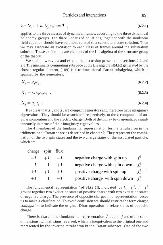
89Particles and Interactions
ˆˆe u em a m
m m ak k + =2 0 , (6.2.1)
applies to the three classes of dynamical frames, according to the three dynamicalholonomy groups. The three linearized equations, together with the nonlinearfield equation should have solutions related to a substratum state solution. Thenwe may associate an excitation to each class of frames around the substratumsolution. These excitations are elements of the Lie algebra of the structure groupof the theory.
We shall now review and extend the discussion presented in sections 2.2 and2.3.The maximally commuting subspace of the Lie algebra sl(4,) generated by thechosen regular element, [109] is a tridimensional Cartan subalgebra, which isspanned by the generators:
X k k=1 1 2 , (6.2.2)
X k k k k=2 0 1 2 3 , (6.2.3)
X k k=3 0 3 . (6.2.4)
It is clear that X1, and X2 are compact generators and therefore have imaginaryeigenvalues. They should be associated, respectively, to the z-component of an-gular momentum and the electric charge. Both of them may be diagonalized simul-taneously in terms of their imaginary eigenvalues.
The 4 members of the fundamental representation form a tetrahedron in thetridimensional Cartan space as described in chapter 2. They represent the combi-nation of the two spin states and the two charge states of the associated particle,which are:
charge spin flux negative charge with spin up
negative charge with spin down positive charge with spin up
positive charge with spin down
f
f
f
f
-
-
+
+
- + -- - ++ +++ --
1 1 11 1 11 111 11
.
The fundamental representation f of SL(2,), indicated by f+, f+
, f-, f-
groups together two excitation states of positive charge with two excitation statesof negative charge. The presence of opposite charges in a representation forcesus to make a clarification. To avoid confusion we should restrict the term chargeconjugation to indicate the original Dirac operation to relate states of oppositecharge.
There is also another fundamental representation f dual to f and of the samedimensions, with all signs reversed, which is inequivalent to the original one andrepresented by the inverted tetrahedron in the Cartan subspace. One of the two

Chapter 6 ENERGY OR MASS AND INTERACTION90
representations is arbitrarily assigned to represent the physical excitation. Themathematics of the representation algebra indicates that the state may also bedescribed as composed of 3 members of its dual representation. In turn, the dualrepresentation may also be similarly described as composed of 3 members of itsdual, which is the original representation. This mutual decomposition is reminis-cent of the idea of “nuclear democracy” proposed in the 1960’s [110] but re-stricted to dual representations. To avoid confusion we restrict the use of the termduality to relate these inequivalent representations.
In standard particle language the antiparticle is the dual particle which impliesthat it also is the charge conjugate. Nevertheless, this assignment of a physicalparticle-antiparticle pair to the fundamental representation and its inequivalentdual is not a mathematical implication of standard particle theory, it is only aphysical assumption. Since our fundamental representation includes oppositecharges it is not appropriate to consider the dual representation as antiparticles.We may, as well, simply say that the antiparticle is determined by the algebraconjugation. The dual particle is just a necessary dual mathematical structure.
We have then for a particular state p of the fundamental representation,
( ) ( )p f f f f q q q + + + - + + -º = º , (6.2.5)
in terms of the dual states q. Similarly for a particular q state,
( ) ( )q q q q p p p + + + - + + -= = . (6.2.6)
It does not follow that the q necessarily are states of a different physicalexcitation, only that the q form a dual triplet mathematical representation of the prepresenting the same excitation. This allows a different physical interpretationfor these mathematical constructions. It should be noted that all p, q have electriccharge equal to the geometric unit, electron charge e. Since these excitationshave particle properties, there is a dual mathematical representation of the physi-cal excitation (particle). We may raise the following question? What happens if wephysically identify p with the proton, which mathematically may be expressed as3 q, interpreted as quarks? In our theory there is no need to assign fractionalcharges to quarks. In accordance with the “restricted nuclear democracy” we mayassume that the quark states, in turn, may be mathematically expressed as 3 pro-tons p, which may justify the large experimental mass of these unstable dualstates.
The fundamental representation of Sp(2,) which may be displayed as a squarein a two dimensional Cartan space is e-
, e-, e+
, e+. Its dual Sp(2,) representa-
tion, obtained by reversing all signs is mathematically the same e+, e+
e-, e-
.Similarly the SL(2,) representation n, n which may be displayed in a one dimen-sional Cartan space is mathematically its own SL(2,) dual. Therefore, the onlyone of the three excitations with a mathematically inequivalent dual structure is p.Since the Sp(2,) and SL(2,) subgroups may be imbedded in SL(2,), the corre-sponding Cartan spaces of Sp(2,) and SL(2,) may also be imbedded in theCartan subspace of SL(2,). The plane subspace Q=-1, including dual states, hascharges of one definite sign and is a representation of Sp(2,). Another plane,

91Particles and Interactions
Q=1, containing opposite charges is another representation of Sp(2,) whichcompletes the SL(2,) Cartan subspace.
The space SL(4,)/SU(2)SU(2) is a nonadimensional riemannian space of thenoncompact type. There are 9 boost generators Bm
a. The rotation SU(2), indicatedby S, contained in in the maximal compact SO(4) acts on the m index and theelectromagnetic SU(2), indicated by Q, contained in SO(4) acts on the a index,
a n m mb a n bQ B S B ¢= . (6.2.7)
Similarly the subspace Sp(4,)/SU(2)U(1) is a hexadimensional riemannian spaceof the noncompact type. The complementary subspace within SL(4,)/SU(2)SU(2)is 3-dimensional. There is a triple infinity of these subspaces within the totalspace, reflecting the triple infinity of groups P in G, depending on the choice of anelectromagnetic generator among the three possible ones in SU(2).
In Sp(4,)/SU(2)U(1), with a fixed electromagnetic generator, we have a vec-tor in the odd sector, representing a momentum k associated to an excitation e.Since we have this situation in SL(4,)/SU(2)SU(2) for each generator in SU(2),we have, in effect, 3 momenta, ki, which may characterize an excitation p. We mustconsider excitations characterized by 3 momenta, ki, which may be interpreted asthree subexcitations. This effect was used in the previous chapter to calculatequantum corrections to the proton and neutron magnetic moments.
Three P-subexcitations are necessary to characterize the protonic excitation p, butnot those of e nor those of n. Mathematically we have a system characterized by 3trimomenta, ki, which may be scattered into another system of 3 trimomenta, kj’. Ascattering analysis of excitations must include all momenta in some d functions whichappear in the scattering results. Experimentally this is a collision with a system of 3pointlike scattering centers and is interpreted as a collision with partons inside theproton. In general it is clear that a pointlike proton excitation is not predicted by ourtheory. In particular, e scattering from p can be replaced by a sum of incoherent scatter-ings from P-excitations. Then group invariance implies that the collision cross sectioncan be expressed as two functions of the energy and momentum transfer and, for deepscattering, Bjorken’s scaling law is obtained.
6.3. Interpretation as Particles andInteractions.
We have found properties of the geometric excitations which are particlelike.We take the position that this is no coincidence but indicates a geometrical struc-ture for physics. The source current J depends on a frame. To each holonomygroup we may associate a class of frames thus giving three classes of matter.
As already discussed in section 5.8, the corresponding L-frame represents azero bare mass, neutral, spin ½, left handed pointlike geometric excitation, whichobeys eq. (5.8.1). It has the particle properties of the neutrino.
For the P-potential, the corresponding P-frame represents a massive, negativecharge -1, spin ½, geometric pointlike excitation with bare magnetic g-factor -2,which obeys the Dirac equation. It has the properties of the electron.
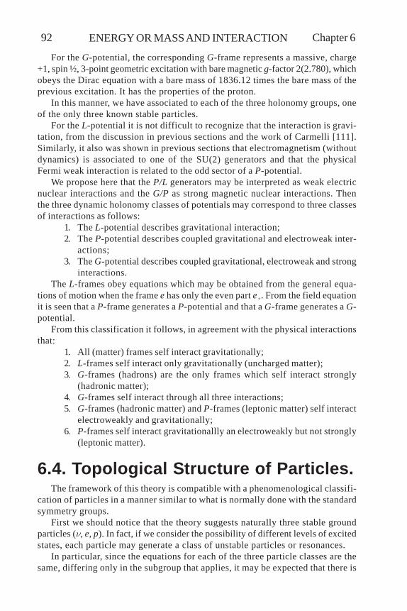
Chapter 6 ENERGY OR MASS AND INTERACTION92
For the G-potential, the corresponding G-frame represents a massive, charge+1, spin ½, 3-point geometric excitation with bare magnetic g-factor 2(2.780), whichobeys the Dirac equation with a bare mass of 1836.12 times the bare mass of theprevious excitation. It has the properties of the proton.
In this manner, we have associated to each of the three holonomy groups, oneof the only three known stable particles.
For the L-potential it is not difficult to recognize that the interaction is gravi-tation, from the discussion in previous sections and the work of Carmelli [111].Similarly, it also was shown in previous sections that electromagnetism (withoutdynamics) is associated to one of the SU(2) generators and that the physicalFermi weak interaction is related to the odd sector of a P-potential.
We propose here that the P/L generators may be interpreted as weak electricnuclear interactions and the G/P as strong magnetic nuclear interactions. Thenthe three dynamic holonomy classes of potentials may correspond to three classesof interactions as follows:
1. The L-potential describes gravitational interaction;2. The P-potential describes coupled gravitational and electroweak inter-
actions;3. The G-potential describes coupled gravitational, electroweak and strong
interactions.The L-frames obey equations which may be obtained from the general equa-
tions of motion when the frame e has only the even part e+. From the field equationit is seen that a P-frame generates a P-potential and that a G-frame generates a G-potential.
From this classification it follows, in agreement with the physical interactionsthat:
1. All (matter) frames self interact gravitationally;2. L-frames self interact only gravitationally (uncharged matter);3. G-frames (hadrons) are the only frames which self interact strongly
(hadronic matter);4. G-frames self interact through all three interactions;5. G-frames (hadronic matter) and P-frames (leptonic matter) self interact
electroweakly and gravitationally;6. P-frames self interact gravitationallly an electroweakly but not strongly
(leptonic matter).
6.4. Topological Structure of Particles.The framework of this theory is compatible with a phenomenological classifi-
cation of particles in a manner similar to what is normally done with the standardsymmetry groups.
First we should notice that the theory suggests naturally three stable groundparticles (n, e, p). In fact, if we consider the possibility of different levels of excitedstates, each particle may generate a class of unstable particles or resonances.
In particular, since the equations for each of the three particle classes are thesame, differing only in the subgroup that applies, it may be expected that there is

93Particles and Interactions
some relation among corresponding levels of excitations for each class, formingfamilies.
The ratio of the mass of the hadron in the ground level family (proton) to themass of the lepton in the ground level family (electron) has been calculated fromthe ratio of volumes of coset spaces based on the existence of a inert nonzeroconstant solution for the substratum potential. This inert solution is the represen-tative of a class of equivalent solutions generated by the action of the structuregroup.
Now consider only topological properties, independent of the potential, of thespace of complete solutions (substratum plus excitation solutions). Scatteringprocesses of excitations around a given substratum should naturally display theseproperties. An incoming scattering solution is a jet bundle local section, over aworld tube in the space-time base manifold, which describes the evolution of thesolution in terms a timelike parameter t from past infinity to some finite time t.Similarly, an outgoing solution is a local section from time t to future infinity. Thelocal sections in the bundle represent classes of solutions relative to local ob-servers. Scattering solutions at infinity are asymptotically free excitation solu-tions around a substratum. The substrata (incoming and outgoing) are equivalentto each other and to the constant inert solution if we choose observer framesadapted to the substrata.
The equations are of hyperbolic type and we should provide initial conditions,at past infinity t=-¥, for the solutions over an initial tridimensional spatial hy-persurface -. We require that any incoming solution over the past infinity hyper-surface - reduce to a free excitation around the substratum solution over thebidimensional subspace -(¥) at spatial infinity r=¥. Since the incoming solu-tion substrata are equivalent to the inert substratum solution at spatial infinity-
(¥), we may treat this spatial infinity as a single point, thus realizing a singlepoint compactification of -, so the initial hypersurface - is homeomorphic toS3. All incoming solutions on - are classified by the functions over S3. The samerequirements may be applied to the outgoing remote future solutions and, in fact,to any solution along an intermediate tridimensional hypersurface , a section ofthe world tube. Thus, the final hypersurface at future infinity + is also homeo-morphic to S3. The incoming and outgoing substratum local sections over - and+ must be pasted together in some common region around the present t, by thetransition functions of the bundle. The scattering interaction is represented bythe group action of the transition functions at t=0. All generators of the groupproduce a transformation to a different, but equivalent under the group, expres-sion for the solution. If the holonomy group of the solution is not the wholegroup, there is a reference frame which reduces the structure group to the particu-lar holonomy subgroup. But in general for arbitrary observers, there are solutionsformally generated by SL(2,)=SL(4,). Since this transition region, the “equa-tor” ´R, has the topology of S3´R, the transition functions j define a mapping, atthe t=0 hypersurface,
: ( , )S SLj 3 2 , (6.4.1)
which is classified by the third homotopy group [112] of the structure group

Chapter 6 ENERGY OR MASS AND INTERACTION94
SL(2,) or the respective holonomy subgroup. There are some solutions not de-formable to the inert solution by a homeomorphism because j represents thetwisting of local pieces of the bundle when glued together.
The homotopy group of SL(2,) is Z ZÄ [9].Similarly the homotopy group forboth Sp(2,) and SL(2,) is Z. The scattering solutions are characterized by topo-logical quantum integer numbers n, for the three groups, and n’ only for group G,called winding or wrapping numbers. In all cases the scattering solutions arecharacterized by one topological winding number n and in particular the hadronicscattering solutions have an additional topological winding number n’. This re-sult implies that there are solutions wn, en that are not homotopically equivalent tow0, e0.
All p, e, n excitation solutions with a given n may be associated among them-selves because of the isomorphism of the homotopy groups Z. This is an equiva-lence relation. Two p, e, n excitation with the same n are in the same topologicalclass determined by the substratum. Each topological class, characterized by thetopological quantum number n defines a physical class, a family of particles withthe same winding number, which is respected by transitions the same as the alge-braic quantum numbers s, q, f.
For example, the association of a solution of each type to any value of n maybe part of a general scheme of relations labeled by n as follows:
, , ,
e l
e
l e l l
h p h p hm
m
m tn n n n n n
= = == = == =
0 1 2
0 1 2
0 1 2
, (6.4.2)
among the excitation levels of the electron (proper leptons), the excitation levelsof the neutrino (other neutrinos) and the excitation levels of the proton (hadrons).
In any case, the possibility exists that there be excited states which may beinterpreted as a particle composed of p, e and n . As a matter of fact Barut [113]suggested that the muon should be considered as an electromagnetic excitationof the electron. Although the details should be different, because Barut’s ap-proach is only electromagnetic in nature and ours is a unified interaction, we mayconjecture also that the muon is an excited electron state with a leptonic windingnumber n=1. Similarly the t would be an excitation with winding number n=2
6.5. Geometric Excitation Masses.If the leptons are topological excitations it should be possible to calculate
their mass ratios [114] using the method given in chapter 4. The integrand JG ineq. (4.1.10), which corresponds to a fundamental representation, is a local sub-stratum constant equal for all values of n. The number of possible states of afundamental representation only depends on the integration volume. Physically,when integrating over the CR subspace of De Sitter space C, corresponding toinequivalent observer states by an L transformation, we have counted the numberof L equivalence classes of states (points in the mass hyperboloid are in the same

95Particles and Interactions
relativistic equivalence class as the rest state of the representation) in local form(only counting n=0 local states). Taking in consideration the global characteris-tics of the topological excitation which would represent heavy leptons, the countshould be larger, over all L equivalence classes of excitation states with wrappingn. What is the number of states for each value of n?
Since we are working with a manifold with atlas, the integration over the sym-metric space K is realized on the atlas charts. On the principal fiber bundle (E,M,G),the transition function preserves the projection and acts, as a group element, overthe fiber which is the bundle structure group G [9]. For two neighborhoods U, V inthe base manifold M, which corresponds to space-time, we have the followingmaps: homeomorphisms h from the bundle to the model space, transition func-tions j among the charts and partial identity i over the points mM.
The transition function j acts as an element of G over the incoming scatteringsolution, defined on a hypersurface homeomorphic to S3, to produce the outgoingscattering solution. Physically j represents a collision interaction. The active repre-sentation is the interaction of two excitations observed by a single observer. Thepassive representation is the observation of a single excitation by different ob-servers. The nontrivial transition functions of class [jn], where the index n repre-sents the set of wrapping numbers (n, n’), are classified by the mappings. Con-sider G as a principal fiber bundle (G,K,G+). The induced representations, assignedto points mM, are sections of an associated bundle to G that has Lorentz grouprepresentations [L] as fiber and is denoted by (D,K,[L],L) as shown in chapter4. Under a change of charts, representing a change of observers, the transitionfunction acts on the bundle D (fig. 2) on the section JG over K, which we shallindicate by f(m).
The transition functions belong to the different classes determined by thethird homotopy group of G. The class [jn] may be expressed, using the homotopicproduct [115] in terms of the class [j1]. This class [jn] may be considered gener-ated by the product of n independent elements of class [j1] and one element ofclass [j0]. Observe that the homotopic mapping essentially determines a wrap-ping of subspaces s(m)G, wrappings homeomorphic to spheres S3, inside (G,K,G+).Each of the generating classes j is globally associated to a generating wrappedsubspace s in (G,K,G+), additional and necessary, linked to the original inert sub-space by a transition function. In this manner the class [jn] is associated to thetrivial wrapping [s0] and to (n, n’) additional wrappings [s1], defined by the expres-sion for the coordinates u of point mM.
The excitation is not completely described by a single subspace which wouldcorrespond to a single observer s(m) in the passive representation. For globalreasons we must accept the presence of as many images of generating subspacesin the nontrivial chart as there are wrappings. Nevertheless some of the wrap-pings may be equivalent under the subgroup of interest. For the trivial subbundleG there is only one independent wrapping, the trivial (n=0) wrapping s0, becausethe subspaces sn are equivalent under a G transformation. For other subbundles,a tridimensional su(2) subalgebra acts on the complete group G fiber bundle,generating transformations of P and L subbundles which are not equivalent underthe corresponding subgroup. It is possible to generate no more than three wrap-
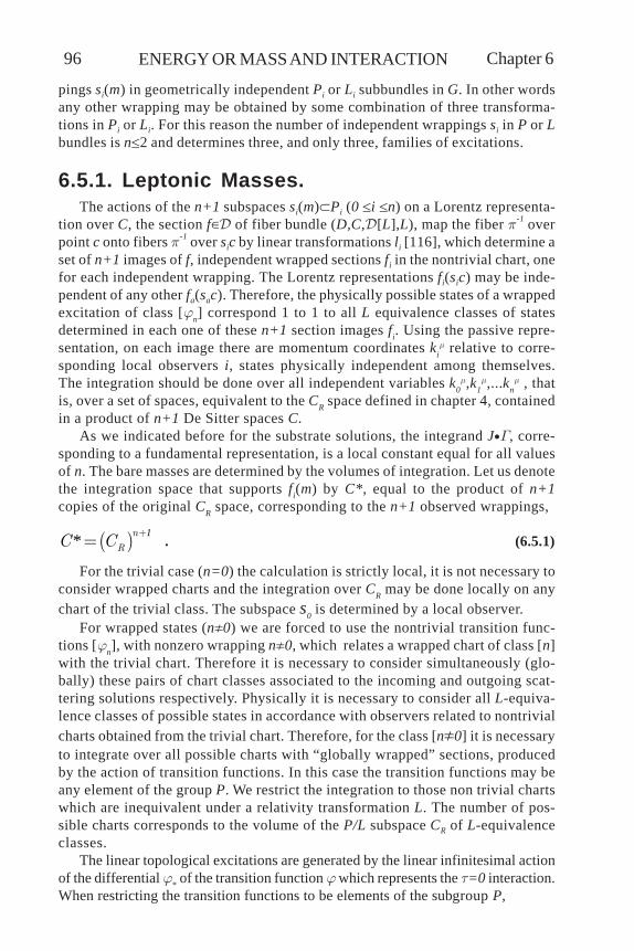
Chapter 6 ENERGY OR MASS AND INTERACTION96
pings si(m) in geometrically independent Pi or Li subbundles in G. In other wordsany other wrapping may be obtained by some combination of three transforma-tions in Pi or Li. For this reason the number of independent wrappings si in P or Lbundles is n2 and determines three, and only three, families of excitations.
6.5.1. Leptonic Masses.The actions of the n+1 subspaces si(m)Pi (0in) on a Lorentz representa-
tion over C, the section f of fiber bundle (D,C,[L],L), map the fiber p-1 overpoint c onto fibers p-1 over sic by linear transformations li [116], which determine aset of n+1 images of f, independent wrapped sections fi in the nontrivial chart, onefor each independent wrapping. The Lorentz representations fi(sic) may be inde-pendent of any other fa(sac). Therefore, the physically possible states of a wrappedexcitation of class [jn] correspond 1 to 1 to all L equivalence classes of statesdetermined in each one of these n+1 section images fi. Using the passive repre-sentation, on each image there are momentum coordinates ki
m relative to corre-sponding local observers i, states physically independent among themselves.The integration should be done over all independent variables k0
m,k1m,...kn
m , thatis, over a set of spaces, equivalent to the CR space defined in chapter 4, containedin a product of n+1 De Sitter spaces C.
As we indicated before for the substrate solutions, the integrand JG, corre-sponding to a fundamental representation, is a local constant equal for all valuesof n. The bare masses are determined by the volumes of integration. Let us denotethe integration space that supports fi(m) by C*, equal to the product of n+1copies of the original CR space, corresponding to the n+1 observed wrappings,
( )* n
RC C+= 1
. (6.5.1)
For the trivial case (n=0) the calculation is strictly local, it is not necessary toconsider wrapped charts and the integration over CR may be done locally on anychart of the trivial class. The subspace s0 is determined by a local observer.
For wrapped states (n0) we are forced to use the nontrivial transition func-tions [jn], with nonzero wrapping n0, which relates a wrapped chart of class [n]with the trivial chart. Therefore it is necessary to consider simultaneously (glo-bally) these pairs of chart classes associated to the incoming and outgoing scat-tering solutions respectively. Physically it is necessary to consider all L-equiva-lence classes of possible states in accordance with observers related to nontrivialcharts obtained from the trivial chart. Therefore, for the class [n0] it is necessaryto integrate over all possible charts with “globally wrapped” sections, producedby the action of transition functions. In this case the transition functions may beany element of the group P. We restrict the integration to those non trivial chartswhich are inequivalent under a relativity transformation L. The number of pos-sible charts corresponds to the volume of the P/L subspace CR of L-equivalenceclasses.
The linear topological excitations are generated by the linear infinitesimal actionof the differential j* of the transition function j which represents the t=0 interaction.When restricting the transition functions to be elements of the subgroup P,

97Particles and Interactions
( )UhV V V P¾¾ = ´ , (6.5.2)
we should only consider the effect of the differential mapping j*. The odd sub-space in the P algebra, as differential mapping, generates the coset C. The onlygenerator inequivalent to an L “boost” is the compact u(1) generator. The differ-ential action produces a smaller space of L-equivalence classes. If we denote thecompact subgroup U(1)SU(2) of P by H we obtain the noncompact coset BC
PB
H= . (6.5.3)
The group P may be expressed as a principal fiber bundle (P,B,H) over B. If weinject L in P, the image of the rotation subgroup in L should be the SU(2) subgroupin H but the image of the “boost” sector in L is not uniquely defined in B. Thegroup L acts on P preserving its image in P. The u(1) subalgebra of H acts on B, asa translation within P, mapping the C subspace onto another subspace C’ in Bwhich is P-equivalent to C. Nevertheless C´ is not L-equivalent to C. Therefore,the possible L-inequivalent states correspond to the translation action by theU(1) compact subgroup not related [115] with the rotation SU(2). The number of L-equivalence classes of these possible charts, over which we should integrate, isdetermined by the volume of this electromagnetic U(1) group. The total wrappedspace CT for an n-excitation (n0) is the space formed by all possible translated,not relativistically equivalent, C* spaces
( ) *TC U C= ´1 . (6.5.4)
The number of states (different k values) is, therefore, proportional to thevolume of this total CT space, which may be calculated,
( ) ( )( ) ( )( ) nTRV C V U V C n
+= ´ ¹
11 0 . (6.5.5)
The bare mass of the trivial excitation (n=0) which is the electron, as previ-ously indicated, is proportional to the volume of CR
( )RV Cp
=16
3 . (6.5.6)
The bare masses corresponding to the n-excitations (n0) are proportional tothe volumes
( ) n
TV C np
p+æ ö÷ç= < £÷ç ÷çè ø
1164 0 23
, (6.5.7)
which may be expressed in terms of the electron bare mass m0,

Chapter 6 ENERGY OR MASS AND INTERACTION98
n
nmn
mp
pæ ö÷ç= < £÷ç ÷çè ø0
16 4 0 23
. (6.5.8)
For excitations with wrappings 1 and 2 we have
( ) . .R
m mV C
m mt
m
p= = = » =2
1
16 16 75516 16 8183
, (6.5.9)
( )
. .
. Mev
m m
m Om
pp
a
æ ö÷ç= = ´÷ç ÷çè ø
= » +
1 016 4 0 5109989 210 5516
3107 5916 , (6.5.10)
( )
. .
. Mev
m m
m Ot
pp
a
æ ö÷ç= = ´÷ç ÷çè ø
= » +
2
2 016 4 0 5109989 3527 825
31802 7 , (6.5.11)
which correspond to the bare masses of the m and t leptons, due to the electro-magnetic U(1) interaction. Due to this electromagnetic interaction in the topologi-cal excitation, we should apply higher order energy corrections to these massesmi. For the subbundle L we can make a similar calculation. The bare masses of theneutrinos for the 3 families are zero because the volume of the L/L coset space iszero, as indicated in section 4.3. We shall refer to these topological excitations,respectively, as TnP-excitations and TnL-excitations.
6.5.2. Mesonic Masses.The chart transformations under general G transition functions translate, within
G, the CR region of integration. The only possible additional L-inequivalent statescorrespond to the action of compact group sectors. In order to find the differentpossibilities we consider the two related chains of symmetric spaces in G, notrelated to L
( ) ( )
( ) ( )
R RG K C I
SU SU U U I
É É É
È È È
É É É2 2 1 1 . (6.5.12)
The compact symmetric subspaces CR and KR, respectively, contain one and twoU(1) electromagnetic subgroups of the three equivalent U(1) subgroups containedin the electromagnetic SU(2)Q. We note that one U(1) is common to both sub-spaces. We are interested in extending the translation within G, beyond the U(1)

99Particles and Interactions
transition function, by adjoining compact sectors. The physical interpretation isthat these excitations are subjected to additional nonlinear interactions whichincrease the energy and therefore their masses. In the same manner as an observ-able relativistic motion increases the rest mass to a kinetic mass, an observablerelativistic interaction increases the free mass to a dynamic mass. This relativisticeffect, included in the mass definition, is realized by the action of the transitionfunctions at t=0.
For n0 topological excitations the transition functions may be extended from U(1)to CR. The physical interpretation is that these topological excitations are subjected tothe additional odd electroweak nonlinear interactions of a leptonic P-system. We saythat the excitations are “masked” by the nonlinear electroweak interactions. Thegeometric mass expressions for the class [n0] masked excitations should be multipliedby the volume of the corresponding complete subspace of L-equivalence classes V(CR)rather than by its subspace V(U(1)). The weak interaction energy acquired by the n-excitations corresponds to the product of the values from equations (6.5.10) and (6.5.11)by the ratio of the volumes,
( )( )( )
.RV Cm mm mV U
p
m
¢= = » =1
1
4 1 32095731
. (6.5.13)
If we use the experimental values for the lepton masses, we obtain the maskedgeometric masses,
( ). Mev m m Op a¢ = » +1 140 8778 , (6.5.14)
( ) Mev fm m O a¢ = » +2 2369 . (6.5.15)
We shall refer to these CR masked (electroweakly interacting) topological excita-tions as TnPC-excitations. The TnPC-excitations may be considered components ofmesons. In particular, a masked muon m’ or T1PC -excitation, joined to a low energyT1L-excitation, has the geometric mass and other properties of the pion p.
For n0 topological excitations the transition functions may be further ex-tended beyond CR to include the sector of KR corresponding to both U(1) oddsubgroups in KR which is an SU(2)/U(1) compact sector which may be identifiedwith the sphere S2. The physical interpretation is that these excitations are sub-jected to the additional strong S2 electromagnetic interaction of a hadronic G-system. The parametrization of group spaces and their symmetric cosets is, to acertain extent, arbitrary. They map different points in the linear Lie algebra to thesame group operation. Since both equivalent U(1) subgroups in S2 have the samesignificance because of the symmetry of S2, they both should contribute equallyto the invariant volume of S2 and it is convenient to choose a parametrizationwhich explicitly displays this fact. A parametrization by the odd generators ac-complishes this,
( ) ( ) ( )( ) exp exp exp ( )SU J J J Ua a a S S+ + - - + -= =3 32 1 , (6.5.16)

Chapter 6 ENERGY OR MASS AND INTERACTION100
( )( ) ( ) ( )( ) ( ) ( )V SU V V U V Vp S S p S+ - += = =2 22 16 1 4 . (6.5.17)
We adjoin the group subspace SKR, defined by the expression in equation (6.5.16),to subspace CR. Because of the extended integration in S, the n-excitations acquire astrong interaction energy corresponding to the ratio of the volumes
( )( )
( ) ( ) . .R K
R
V Cm mV
m V C mp
SS p
¢¢= = = = » =
¢121
1
4 3 5449 3 5371 . (6.5.18)
We obtain the geometric masses for n=1 and n=2,
( ) ( ) ( ). Mev m m V m m Op p KS p a¢¢= = = = +12
1 4 494 76 . (6.5.19)
( ) ( ) Mev K
mm m V m m
mt
m
pS p
æ öæ ö ÷ç÷ç ÷¢¢ ¢ ¢ ç= = » =÷ ÷ç ç÷ç ÷è ø ÷çè ø
12
2 2 116 4 8303
3. (6.5.20)
These excitations are not contained in the P sector defined by the n=0 wrapping,but rather in a combination of inequivalent P sectors inside G. Therefore, strictly,they do not have a proper constituent topological P-excitation. We shall refer tothese odd S masked (strongly interacting) topological excitations as TnPS-excita-tions. In particular, a masked muon m’’ or T1PS-excitation, joined to a low energyT1L-excitation by the strong interaction, has the geometric mass and other proper-ties of the kaon K.
The physical interpretation of these masked leptons suggests that the corre-sponding geometric excitations may be combined to form lepton pairs which maybe considered particles. In accordance with this interpretation, the combinationsunder odd nuclear generators are only possible if there is, at least, one maskedlepton. Take the n=1 topological leptons and construct a doublet l of a cSU(2)combinatory group associating a masked muon and a stable lepton. We shouldindicate that the conjugation in the geometric algebra, which is equivalent to thedual operation in sp(4,), is not the dual operation in csu(2). Both l and its conju-gate are csu(2) fundamental representations 2. The product is
Ä = Å2 2 3 1 . (6.5.21)The first possibility is that m is a weakly masked m’, part of the SU(2) leptonic
system doublet (m’, n) characterized by the charge Q and the muonic number Lm.We get the amplitude for the p representation:
( ) ( )( ), , , ,
, ,
xm n m n p p p
nm m m nn m n m m nn
- +é ùé ù é ù¢ ¢Ä º Åê úë û ë û ë ûé ù¢ ¢ ¢ ¢ ¢ ¢= - Å +ê úë û
0
1 12 2
. (6.5.22)
The only other possibility is the more complex combination where the muon is astrongly masked m’’. In addition to the coupling to n, since m’’ has a strong S2 electro-
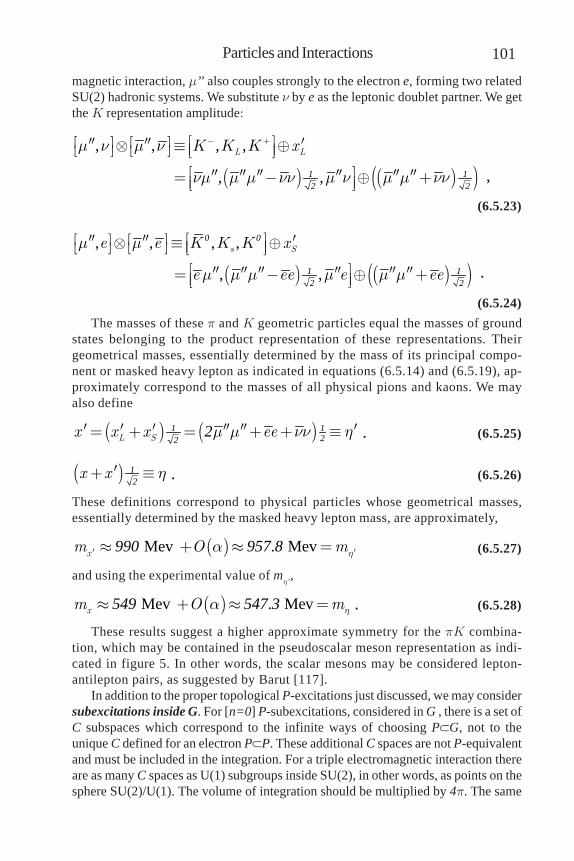
101Particles and Interactions
magnetic interaction, m’’ also couples strongly to the electron e, forming two relatedSU(2) hadronic systems. We substitute n by e as the leptonic doublet partner. We getthe K representation amplitude:
( ) ( )( ), , , ,
, ,
L Lxm n m n K K K
nm m m nn m n m m nn
- +é ùé ù é ù¢¢ ¢¢ ¢Ä º Åê úë û ë û ë ûé ù¢¢ ¢¢ ¢¢ ¢¢ ¢¢ ¢¢= - Å +ê úë û
1 12 2
,
(6.5.23)
( ) ( )( ), , , ,
, ,
s Se e x
e ee e ee
m m K K K
m m m m m m
é ùé ù é ù¢¢ ¢¢ ¢Ä º Åê úë û ë û ë ûé ù¢¢ ¢¢ ¢¢ ¢¢ ¢¢ ¢¢= - Å +ê úë û
0 0
1 12 2
.
(6.5.24)The masses of these p and K geometric particles equal the masses of ground
states belonging to the product representation of these representations. Theirgeometrical masses, essentially determined by the mass of its principal compo-nent or masked heavy lepton as indicated in equations (6.5.14) and (6.5.19), ap-proximately correspond to the masses of all physical pions and kaons. We mayalso define
( ) ( )L Sx x x eem m nn h¢ ¢ ¢ ¢¢ ¢¢ ¢= + = + + º1 122
2 . (6.5.25)
( )x x h¢+ º12 . (6.5.26)
These definitions correspond to physical particles whose geometrical masses,essentially determined by the masked heavy lepton mass, are approximately,
( ) Mev . Mevxm O mha¢ ¢» + » =990 957 8 (6.5.27)
and using the experimental value of mh’,
( ) Mev . Mevxm O mha» + » =549 547 3 . (6.5.28)
These results suggest a higher approximate symmetry for the pK combina-tion, which may be contained in the pseudoscalar meson representation as indi-cated in figure 5. In other words, the scalar mesons may be considered lepton-antilepton pairs, as suggested by Barut [117].
In addition to the proper topological P-excitations just discussed, we may considersubexcitations inside G. For [n=0] P-subexcitations, considered in G , there is a set ofC subspaces which correspond to the infinite ways of choosing PG, not to theunique C defined for an electron PP. These additional C spaces are not P-equivalentand must be included in the integration. For a triple electromagnetic interaction thereare as many C spaces as U(1) subgroups inside SU(2), in other words, as points on thesphere SU(2)/U(1). The volume of integration should be multiplied by 4p. The same

Chapter 6 ENERGY OR MASS AND INTERACTION102
thing happens with L-excitations. In other words, class [n=0] leptonic subexcitationmasses m0, present in a hadronic G-system, are masked by the nonlinear stronginteractions. We shall refer to these S2 masked (strongly interacting) subexcitations asGS-subexcitations. The GS-subexcitations geometric mass values corresponding to thefundamental leptonic excitations are 4p times the previous leptonic geometric massvalues,
( ) ( ), , , , , . , , . , , . , Gevem e m tn m n t n¢¢¢ = 0 00641 0 1 77 0 29 9 0 . (6.5.29)
The masked excitations are characterized by the same quantum numbers whichcharacterize the leptonic excitation but the value of the masked geometric massincludes the energy increase due to the other interactions. If the masked excita-tions were to be ejected (injected) from (to) a G-system they would loose (gain)the energy due to the extra interactions, and they would exit (enter) with the baregeometric mass value, as standard free leptons. There are no observable freeparticles with this GS masked masses. Experimentally this masked mass wouldnever be detected by long-range methods. These masked leptonic subexcitationsbehave as quarks.
In particular, the GS-subexcitations correspond, one to one, to the leptons.These GS-subexcitations determine a hexadimensional space. Consequently anyother possible geometric GS-subexcitation can be expressed as a linear superposi-tion of these fundamental masked geometric subexcitations. Alternately we mayinterpret some of these subexcitations as quark states. The structure of maskedleptonic subexcitations is geometrically equivalent to the physical quark struc-ture. For example, a superposition of 2 low velocity masked electrons e plus 1masked low energy neutrino ne has a 2/3 charge and a total 4.2 Mev invariantmass and may be interpreted as a u quark. Similarly a superposition of 2 maskedlow velocity muons m plus 1 masked low energy neutrino nm has 2/3 charge and1.2 Gev total mass. It should be noted that, if free quarks are unobservable, allexperimental information about their masses comes from bound quark states (me-son resonances) and must depend somehow on theoretical arguments about thesestates. There is no quark confinement problem.
As shown in section 6.2, a proton contains leptonic subexcitations. We mayconsider that there are GS-subexcitations inside the hadrons. In this manner wemay identify six flavors of geometric masked leptonic excitations inside all had-rons providing an equivalent quark flavor structure. There is also another triplestructure associated to the dual representations, also shown in that section, whichcould in principle provide another quark structure. Nevertheless, we have saidduality is just a necessary mathematical equivalent structure. Additionally, thereis no spin-statistics problem with these geometric components and there is noneed for another degree of freedom (color).
6.6. Barut’s Model. On the other hand, Barut has suggested [117, 118, 119, 120, 121] a process to
construct particles in terms of the stable particles and the muon. Therefore, it
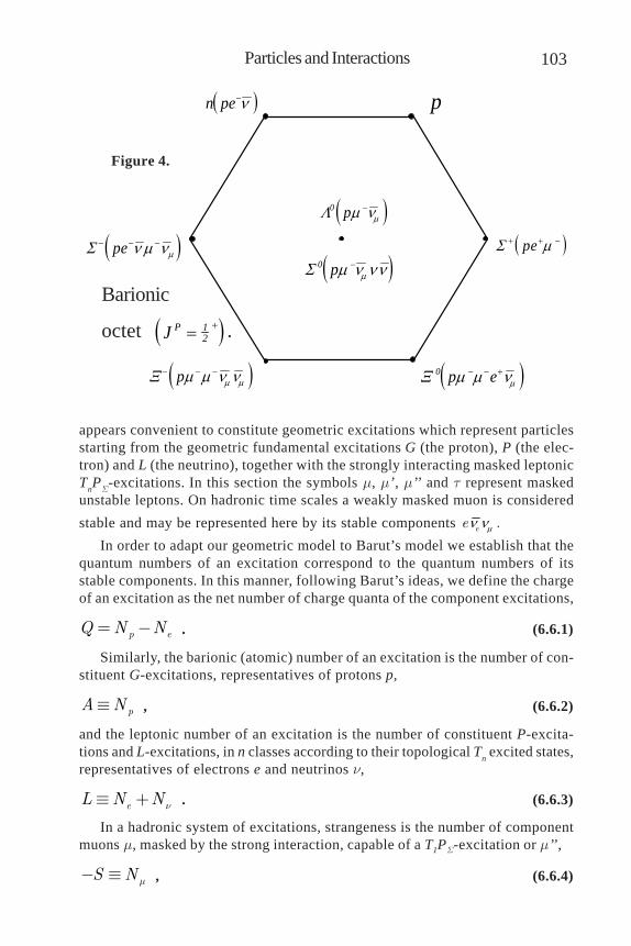
103Particles and Interactions
appears convenient to constitute geometric excitations which represent particlesstarting from the geometric fundamental excitations G (the proton), P (the elec-tron) and L (the neutrino), together with the strongly interacting masked leptonicTnPS-excitations. In this section the symbols m, m’, m’’ and t represent maskedunstable leptons. On hadronic time scales a weakly masked muon is consideredstable and may be represented here by its stable components ee .
In order to adapt our geometric model to Barut’s model we establish that thequantum numbers of an excitation correspond to the quantum numbers of itsstable components. In this manner, following Barut’s ideas, we define the chargeof an excitation as the net number of charge quanta of the component excitations,
p eQ N N= - . (6.6.1)
Similarly, the barionic (atomic) number of an excitation is the number of con-stituent G-excitations, representatives of protons p,
pA Nº , (6.6.2)
and the leptonic number of an excitation is the number of constituent P-excita-tions and L-excitations, in n classes according to their topological Tn excited states,representatives of electrons e and neutrinos n,
eL N N nº + . (6.6.3)
In a hadronic system of excitations, strangeness is the number of componentmuons m, masked by the strong interaction, capable of a T1PS-excitation or m’’,
S N m- º , (6.6.4)
p
pe
p
0 p
0 p
n pe
0 p e
pe
0 p
0 p
Barionic
octet J P 12 .
Figure 4.
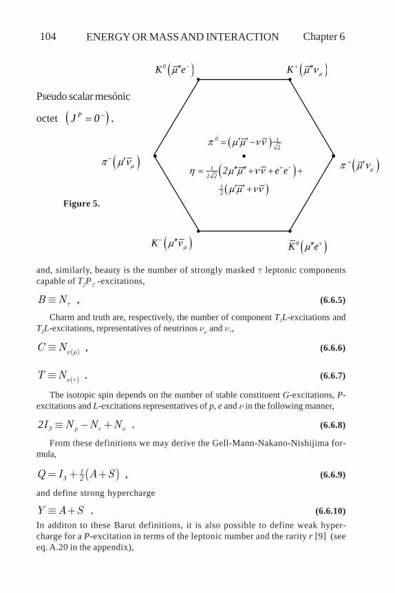
Chapter 6 ENERGY OR MASS AND INTERACTION104
and, similarly, beauty is the number of strongly masked t leptonic componentscapable of T2PS -excitations,
B N tº , (6.6.5)
Charm and truth are, respectively, the number of component T1L-excitations andT2L-excitations, representatives of neutrinos nm and nt,
( )C Nn mº , (6.6.6)
( )T Nn tº . (6.6.7)
The isotopic spin depends on the number of stable constituent G-excitations, P-excitations and L-excitations representatives of p, e and n in the following manner,
p eI N N N nº - +32 . (6.6.8)
From these definitions we may derive the Gell-Mann-Nakano-Nishijima for-mula,
( )Q I A S= + +13 2 , (6.6.9)
and define strong hypercharge
Y A Sº + . (6.6.10)In additon to these Barut definitions, it is also possible to define weak hyper-charge for a P-excitation in terms of the leptonic number and the rarity r [9] (seeeq. A.20 in the appendix),
e e 16
0K e K
K 0K e
0 e e
12 2
12
2 e e
0 12
Pseudo scalar mesónic
octet J P 0 .
Figure 5.

105Particles and Interactions
( )y L rº - + . (6.6.11)
The hadronic states contain protons. In figure 4 we show the barionicoctet JP=1/2+ and in figure 6 the barionic decuplet JP=3/2+. The meson statesare bound states of two leptons ll- as indicated in the mesonic octect JP=0- infigure 5.
Furthermore, the geometric theory allows a discussion of the approximatequantum interaction between two dressed leptonic excitation states forminga system (quarkonium?). We speculate that the nonrelativistic effective po-tential should be similar to the one in QCD because there are similarities ofthe mathematics of the theories. If this were the case, (this has to be shown)the nonrelativistic effective potential would be [122]
( ) aV r kr
r= - + (6.6.12)
and then we may fit the experimental Y excited levels accordingly, as is donein QCD.
The full frame excitation has protonlike properties. Within the geometrictheory the quark excitations are not the fundamental building blocks of mat-ter. They are only subexcitations which are useful and necessary in describ-ing a series of hadronic excitations.
p e
p
pe e 0 pe p pe
0 p e
pe p e
0 p
0 p
Figure 6.
Barionic
decuplet J P 32 .
Chapter 6 ENERGY OR MASS AND INTERACTION106
6.7. Relation with Particle Theory.The geometric triple structure determines various structures compatible with the
quark description. On top of this geometry, as is done in the standard model overthe geometry of special relativity, it is possible to add an approximate structure tohelp in the phenomenological understanding of the physical particles. It is knownthat heavy nuclei may be partially understood by using groups SU(N), U(N), O(N)to associate protons and neutrons in a dynamic symmetric or supersymmetricmanner [123]. This is essentially the use of group theory to study the combina-tions of the two building blocks, protons and neutrons, assumed to form nuclei. Inthe same manner we can use certain groups to describe the combinations of thethree fundamental geometrical building blocks introduced by the physical geom-etry, protons, electrons and neutrinos assumed to form other particles.
We are interested in combining G, P and L excitations. We attach L excitationsto P excitations and then to G excitations. As indicated in section 6.1, this combi-nation may not be done uniquely, rather it depends on the identification of asubgroup H with a subspace in the group fiber bundle space G. Any noncompactgenerator is equivalent to a boost or external symmetry, by the adjoint action of acompact generator. Thus, the compact generators generate an internal symmetryof the combination of excitations.
In particular, the identification of L within P is not unique. The group L may beexpressed as the principal bundle (L,3B,S), where the fiber S is the SU(2)R associ-ated to rotations and 3B is the tridimensional boost symmetric space,
( , )( )R
SLB
SU=3 2
2
. (6.7.1)
The group P may be expressed as the principal bundle (P,6B,SU(1)) where 6B isthe hexadimensional double boost symmetric space,
( , )( ) ( )R Q
SpB
SU U=
Ä6 4
2 1
. (6.7.2)
The choice of the boost sector of L (even generators), inside P, depends on theaction of the U(1) group in the fiber of P, generated by k0, a rotation within thedouble boost sector in P.
[ ],k k k k=0 1 0 12 . (6.7.3)
Mathematically this corresponds to the adjoint action of the only compact gen-erator in the odd quotient P/L.
Similarly, the identification of P inside G is not unique either. The group G maybe expressed as the bundle (G,9B,SQ) where Q is the SU(2)Q associated to chargeand 9B is the nonadimensional triple boost symmetric space,
( , )( ) ( )R Q
SLB
SU SU=
Ä9 4
2 2
. (6.7.4)

107Particles and Interactions
The choice of the boost sectors of L and P sector inside G depends on the actionof the SU(2) in the fiber of G, generated by the compact electromagnetic genera-tors. Mathematically this corresponds to the action of all compact generators inthe quotient G/L. The total internal symmetry of first identifying LP and then(LP)G is the product of the two groups. Therefore, there is an internal symme-try action of a group equal to SU(2)U(1), but different to the subgroups of G, onthe identification of the subgroups in the chain GPL.
There is an induced symmetry on the combination of L and P excitations on Gexcitations corresponding to this SU(2)U(1) symmetry. The action of this combi-natorial group may be interpreted as the determination of the possible combina-tions of L and P excitations to give flavor to states of G and P excitations and thusrelated to the weak interactions.
This SU(2)F group relates electron equivalent P-excitation states or neutrinoequivalent L-excitation states. Clearly at sufficiently high energies the mass ofany excitation kinematically appears very small and its effects on results are smalldeviations from those of a zero mass excitation which always corresponds to anexcitation of the even subgroup or L-excitation. For this reason, at high energies,the even part (left handed part) of a P-excitation may be related to an even L-excitation by an SU(2) transformation. Both corresponding physical leptonic exci-tations, the even part e+ or e0 and n, may be considered members of a doublet,labeled by rarity 0 or weak hypercharge -1, while the odd part e- or e1 is a singletlabeled by rarity 1 or weak hypercharge -2. This weak interaction association ofleptons into hypercharged states has the approximate symmetry SU(2)F. In addition,there is an undetermined orientation of L1 inside G which depends of the action ofSU(2)U(1). Under this approach, the standard physical electromagnetic potential A,the potential of U+(1) in SL1(2,), has an orientation angle within the chiral SU(2)U(1)which should be related to the possible polar angles Q in eq. (4.6.5).
Since our description may be made in terms of the proton representation or,alternately, in terms of its dual quark representation as indicated in section 6.2,we could obtain complementary dual realizations of the relations among differentexperimental results. These are really different perceptions or pictures of the samephysical reality of matter. The proton or G-excitation has a three point structure: itbehaves as if formed by quarks. If we use the quark representation to build otherparticles, we may consider that in G the 3 quark states span a 2 dimensional Cartansubspace. There is a combinatorial unitary symmetry, SU(3), related to this sub-space of a type A3 Cartan space, which may be interpreted as the color of thecombinations of states of G and thus related to strong interactions. States of G-excitations display an SU(3)C symmetry.
In this manner, the physical geometry determines an approximate combinato-rial internal symmetry characterized by the combinatorial symmetry group SC,
( ) ( ) ( )C C FS SU SU U= Ä Ä3 2 1 . (6.7.5)
We combine L-excitations, P-excitations and G-excitations using mathematicaland physical considerations. Any subgroup HG geometrically determines a fiberbundle (G,G/H,H,U). The structure group U of the bundle cannot be uniquely, math-ematically, identified with a fixed H subspace in G. It acts on each equivalent H

Chapter 6 ENERGY OR MASS AND INTERACTION108
subspaces, while the fiber is transported throughout the G/H space, and representsan equivalence class of subspaces. We may interpret U as a different group isomor-phic to each H. Mathematically, we require that the combinations of GPL chainsubgroups be realized as direct products. Nevertheless from the physical point ofview we recognize that all chain subgroups are related. The compact SU(2)S spinsubgroup in L is interpreted as physical rotations. The other two compact subgroupsin P and G are U(1) and SU(2)Q and are interpreted as internal electromagnetic rota-tions. The complementary noncompact sectors are interpreted as generalized (inter-nal) boosts. Physically we require that quantum numbers of product representationsin the chain GPL obey an addition rule. As indicated in previous sections, combi-nations of excitations appear to determine masses, magnetic moments, quantum num-bers, etc. of physical particles. The neutron and the pion would correspond, respec-tively, to the fundamental combinations of the GPL and PL chains.
The constructions discussed in this section should share certain features andresults with the standard model while there would be differences in some other fea-tures. This actually represents a program to be carried out. It is true that the standardmodel [112] has led to success, but this does not imply there is no better way ofreordering the physical withot large number of empirical parameters. Other geometricmodels, like string theories [124] involve a large number of dimensions which are notclearly related to a fundamental underlying theoretical physical interaction. Due tothe richness and vastness of particle physics experimental results, it is not clear howdifferences compare with experiments, in particular because the geometrical ideas andthe group SL(4,) [125] may introduce a rearrangement of experimental results.
6.8. Results.The interaction may be classified into three subclasses by the dynamical holonomy
groups of the possible physical potentials. The three classes correspond to gravita-tion, electro-weak and strong physical interactions. Solutions to the three correspond-ing frame excitation equations representing matter, show algebraic and topologicalquantum numbers. The algebraic numbers correspond to electric charge, spin andmagnetic flux. The topological numbers correspond to wrapping (winding) numbersof higher levels of excitation, defining three 2-member leptonic families. We are able toidentify three classes of fundamental excitations, corresponding to the three stablephysical particles: neutrino, electron and proton. The calculated masses agree withthe experimental values.
The bare masses of the leptons in the three families are calculated as topologicalexcitations of the electron in agreement with experimental values. The masses of theseexcitations increase under the action of a strong potential (relativity of energy)producing the meson masses, also in agreement with experiment. The geometrydetermines the geometric excitation mass spectrum, which for low masses, essentiallyagrees with the physical particle mass spectrum. The proton shows a triple structurewhich may be related to a quark structure. The combinations of the three fundamentalgeometric excitations (associated to the proton, the electron and the neutrino), formingother excitations, may be used to represent particles and show a symmetry under thegroup SU(3)SU(2)U(1).

7. Gravitation and Geometry.The standard geometrical approach to gravitation requires the construction of
an energy momentum or stress energy tensor T determined by the classical equa-tions of macroscopic matter and fields. In general these matter fields are describedby the classical fluid equations. It may be claimed that these stress energy ten-sors are not truly geometrical. Einstein [126] himself was unsatisfied by thenongeometrical character of T and spent his later years looking for a satisfactoryunified theory. Now we use the geometrical theory to obtain the Eintein equationswith a geometric stress energy tensor.
It is also known that the value of the fine structure constant a is essentiallyequal to an algebraic expression in terms of p and entire numbers which is relatedto the quotient of the volume of certain groups. Here we determine this expressionusing the invariant measure defined by the substratum solution of this geometri-cal theory.
7.1. Einstein’s Equation.The equation for the total generalized energy (1.2.8) has the structure
ˆ ˆtr F F u F F Xmn m klrn r kl
é ù- =ê úë û4(7.1.1)
of a sum of terms, each of the form corresponding to the electromagnetic stressenergy tensor. Using this equation we may define a tensor with the structure ofstress energy. It is clear that this tensor would not represent the source term ofthe field equations. It represents the energy of the interaction potential and matterframe fields.
Eq. (1.4.3) indicates that the even part of the curvature in this equation repre-sents the classical interaction fields of gravitation and electromagnetism. Due tothis reason we shall separate the terms in the equations with respect to the evensubalgebra and its coset space. In particular, the SL(2,C) curvature form corre-sponds to the Riemann curvature R in standard spinor formulation. It obeys fieldequations which are different from Einstein’s equations and represent a spinorgravitational formulation which resembles Yang’s [18] theory restricted to itsSO(3,1) subgroup.
Yang’s gravitational theory may be seen as a theory of a connection orpotential in the principal bundle of linear frames TMm with structure groupGL(4,). In Yang’s theory the group is taken to act on the tangent spaces to Mand therefore is different from the theory under discussion. The potential inYang’s theory is not necessarily compatible with a metric on the base space M,which leads to well known difficulties. Nevertheless, when Yang’s theory isrestricted to its SO(3,1) subgroup its metrical problems are eliminated. The wellknown homomorphism between this group and our even subgroup SL(2,)establishes a relation between these two restrictions of the theories.
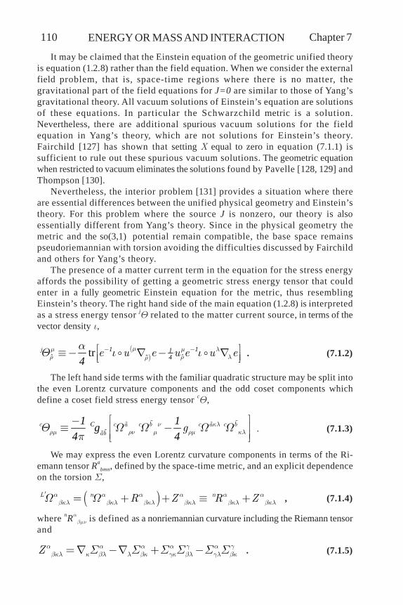
Chapter 7 ENERGY OR MASS AND INTERACTION110
It may be claimed that the Einstein equation of the geometric unified theoryis equation (1.2.8) rather than the field equation. When we consider the externalfield problem, that is, space-time regions where there is no matter, thegravitational part of the field equations for J=0 are similar to those of Yang’sgravitational theory. All vacuum solutions of Einstein’s equation are solutionsof these equations. In particular the Schwarzchild metric is a solution.Nevertheless, there are additional spurious vacuum solutions for the fieldequation in Yang’s theory, which are not solutions for Einstein’s theory.Fairchild [127] has shown that setting X equal to zero in equation (7.1.1) issufficient to rule out these spurious vacuum solutions. The geometric equationwhen restricted to vacuum eliminates the solutions found by Pavelle [128, 129] andThompson [130].
Nevertheless, the interior problem [131] provides a situation where thereare essential differences between the unified physical geometry and Einstein’stheory. For this problem where the source J is nonzero, our theory is alsoessentially different from Yang’s theory. Since in the physical geometry themetric and the so(3,1) potential remain compatible, the base space remainspseudoriemannian with torsion avoiding the difficulties discussed by Fairchildand others for Yang’s theory.
The presence of a matter current term in the equation for the stress energyaffords the possibility of getting a geometric stress energy tensor that couldenter in a fully geometric Einstein equation for the metric, thus resemblingEinstein’s theory. The right hand side of the main equation (1.2.8) is interpretedas a stress energy tensor jQ related to the matter current source, in terms of thevector density i,
()ˆ ˆˆtrj e u e u e u emm m l
r r lr
aQ i i- -é ùº - - ê úë û
1 1144
. (7.1.2)
The left hand side terms with the familiar quadratic structure may be split intothe even Lorentz curvature components and the odd coset components whichdefine a coset field stress energy tensor cQ,
c c a c b c a c bab
gn klrm rn m rm klQ W W W W
pé ù-ê úº -ê úë û
C1 1g4 4
. (7.1.3)
We may express the even Lorentz curvature components in terms of the Ri-emann tensor Ra
bmn, defined by the space-time metric, and an explicit dependenceon the torsion S,
( )L n nR Z R Za a a a a abkl bkl bkl bkl bkl bklW W¢ = + + º + , (7.1.4)
where nRabmn is defined as a nonriemannian curvature including the Riemann tensor
and
Z a a a a g a gbkl k bl l bk gk bl gl bkS S S S S S= - + - . (7.1.5)
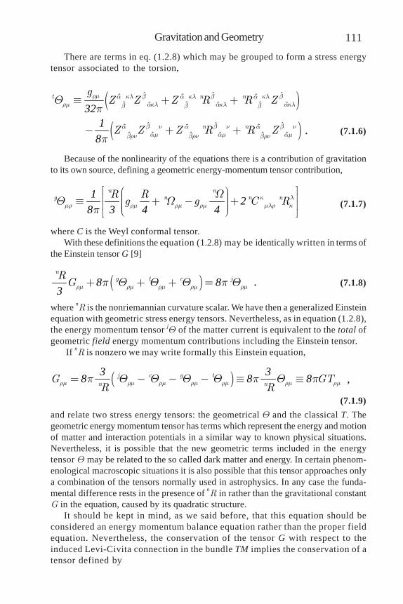
111Gravitation and Geometry
There are terms in eq. (1.2.8) which may be grouped to form a stress energytensor associated to the torsion,
( )
( )
ˆ ˆ ˆˆ ˆ ˆˆ ˆ ˆˆ ˆ ˆ
ˆ ˆ ˆˆ ˆ ˆˆ ˆ ˆˆ ˆ ˆ
t n n
n n
gZ Z Z R R Z
Z Z Z R R Z
rm a kl b a kl b a kl brm akl akl aklb b b
a b n a b n a b nam am ambrn brn brn
Qp
p
º + +
- + +
321
8 . (7.1.6)
Because of the nonlinearity of the equations there is a contribution of gravitationto its own source, defining a geometric energy-momentum tensor contribution,
n ng n n nR R
g g C Rk lmr rm rm rm mlr k
WQ W
p
é ùæ ö÷çê ú÷º + - +ç ÷ê úç ÷çè øë û
1 28 3 4 4 (7.1.7)
where C is the Weyl conformal tensor.With these definitions the equation (1.2.8) may be identically written in terms of
the Einstein tensor G [9]
( )n
g t c jRGrm rm rm rm rmp Q Q Q p Q+ + + =8 8
3 . (7.1.8)
where nR is the nonriemannian curvature scalar. We have then a generalized Einsteinequation with geometric stress energy tensors. Nevertheless, as in equation (1.2.8),the energy momentum tensor jQ of the matter current is equivalent to the total ofgeometric field energy momentum contributions including the Einstein tensor.
If nR is nonzero we may write formally this Einstein equation,
( )j c g tn n
G GTR Rrm rm rm rm rm rm rmp Q Q Q Q p Q p= - - - º º3 38 8 8 ,
(7.1.9)and relate two stress energy tensors: the geometrical Q and the classical T. Thegeometric energy momentum tensor has terms which represent the energy and motionof matter and interaction potentials in a similar way to known physical situations.Nevertheless, it is possible that the new geometric terms included in the energytensor Q may be related to the so called dark matter and energy. In certain phenom-enological macroscopic situations it is also possible that this tensor approaches onlya combination of the tensors normally used in astrophysics. In any case the funda-mental difference rests in the presence of nR in rather than the gravitational constantG in the equation, caused by its quadratic structure.
It should be kept in mind, as we said before, that this equation should beconsidered an energy momentum balance equation rather than the proper fieldequation. Nevertheless, the conservation of the tensor G with respect to theinduced Levi-Civita connection in the bundle TM implies the conservation of atensor defined by

Chapter 7 ENERGY OR MASS AND INTERACTION112
nGR
rmrm
r r
Qp
æ ö÷ç ÷ = =ç ÷ç ÷çè ø38 0 . (7.1.10)
There should be compatibility of the resultant equations with those obtainedfrom the conservation of the current J, which determine the equations of motion,[9]. If the stress energy tensor is decomposed in terms of a multipole expansionwe find the usual equations of motion [7, 132]: geodesic equation for a monopole,equations for a spinning particle and other multipole equations of motion.
For the case of a pure metric gravitation theory there are zero coset fieldsand zero torsion. We have then
j g mGR R 3 38 8 (7.1.11)
where we have defined the matter current energy momentum tensor mQ.When we consider the external field problem, that is, space-time regions
where there is no matter current, the gravitational part of the field equations forJ=0 are similar to those of Yang’s gravitational theory. Only gQ remains and weget back the Stephenson-Yang equation for vacuum. All vacuum solutions ofEinstein’s equation are solutions of these equations. In particular theSchwarzchild metric is a solution and, therefore, the newtonian motion under a1/r gravitational potential is obtained as a limit of the geodesic motion underthe proposed equations. Nevertheless, in the interior field problem there aredifferences between the unified physical geometry and Einstein’s theory.
7.1.1. Newtonian G and the Schwarzschild Mass.
It is usual to assume, as a newtonian approximation of the interior problem,that the characteristic parameters of a newtonian solution of Einstein’sequation v/c1, j1 are of the same order e2 [133] in a small dimensionlessparameter e. This small parameter e may be related to the orthonormal tetradu, thus characterizing the propagation of gravitational disturbances. Thegeometric formulation of Newton’s gravitation is the Newton-Cartan theory [134].The newtonian limit of Einstein type theories of gravitation was previouslydiscussed [9]. The main mathematical difficulty in obtaining the limit is that thegeometric Newton gravitation does not provide a metric but relies on anonriemannian affine connection, a tensor of valence (2,0) and rank 3 (singularmetric) and a scalar time function. There [9] it is shown that, in the limit e0,the metric becomes singular in e. Nevertheless the connection remainsregular in the limit and defines a newtonian affine connection not related toa metr ic . S ince we have taken the connect ion as the fundamenta lrepresentation of gravitation, the gravitational l imit may be definedappropriately as the limit of the connection. The corresponding newtoniancurvature tensor is the limit of the Riemann tensor. The projection of thistensor on the tridimensional time hypersurfaces t defines a Riemann tensor
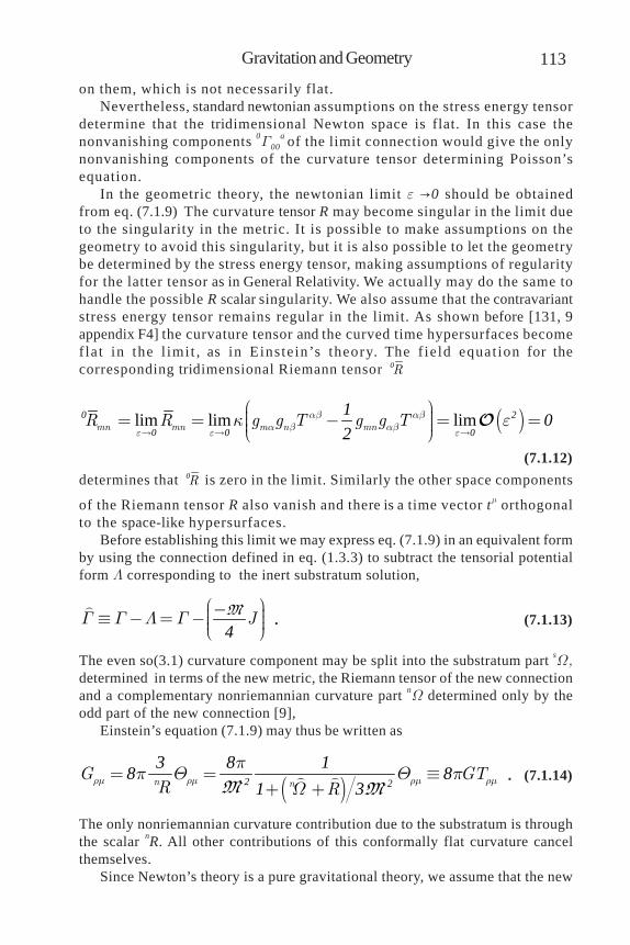
113Gravitation and Geometry
on them, which is not necessarily flat.Nevertheless, standard newtonian assumptions on the stress energy tensor
determine that the tridimensional Newton space is flat. In this case thenonvanishing components 0G00
a of the limit connection would give the onlynonvanishing components of the curvature tensor determining Poisson’sequation.
In the geometric theory, the newtonian limit e0 should be obtainedfrom eq. (7.1.9) The curvature tensor R may become singular in the limit dueto the singularity in the metric. It is possible to make assumptions on thegeometry to avoid this singularity, but it is also possible to let the geometrybe determined by the stress energy tensor, making assumptions of regularityfor the latter tensor as in General Relativity. We actually may do the same tohandle the possible R scalar singularity. We also assume that the contravariantstress energy tensor remains regular in the limit. As shown before [131, 9appendix F4] the curvature tensor and the curved time hypersurfaces becomeflat in the l imit , as in Einstein’s theory. The f ie ld equat ion for thecorresponding tridimensional Riemann tensor R0
( )lim lim limmn mn m n mnR R g g T g g Tab aba b abe e e
k e
æ ö÷ç= = - = =÷ç ÷çè ø0 2
0 0 0
1 02
(7.1.12)determines that R0 is zero in the limit. Similarly the other space components
of the Riemann tensor R also vanish and there is a time vector tm orthogonalto the space-like hypersurfaces.
Before establishing this limit we may express eq. (7.1.9) in an equivalent formby using the connection defined in eq. (1.3.3) to subtract the tensorial potentialform L corresponding to the inert substratum solution,
JG G L Gæ ö- ÷çº - = - ÷ç ÷çè ø4
M . (7.1.13)
The even so(3.1) curvature component may be split into the substratum part sW,determined in terms of the new metric, the Riemann tensor of the new connectionand a complementary nonriemannian curvature part nW determined only by theodd part of the new connection [9],
Einstein’s equation (7.1.9) may thus be written as
( )n nG GT
R Rrm rm rm rm
pp Q Q p
W= = º
+ +2 2
3 8 18 81 3
M M
. (7.1.14)
The only nonriemannian curvature contribution due to the substratum is throughthe scalar nR. All other contributions of this conformally flat curvature cancelthemselves.
Since Newton’s theory is a pure gravitational theory, we assume that the new
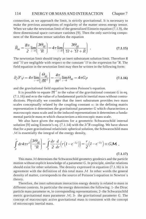
Chapter 7 ENERGY OR MASS AND INTERACTION114
connection, as we approach the limit, is strictly gravitational. It is necessary tomake the previous assumptions of regularity of the matter stress energy tensor.When we take the newtonian limit of the generalized Einstein equation (7.1.9), thethree dimensional space curvature vanishes [9]. Then the only surviving compo-nent of the Riemann tensor satisfies the equation
ˆ ˆ ˆ ˆlim limn s n
RR Re e
Q Qpp
W W
æ ö æ ö÷ ÷ç ç÷ ÷= =ç ç÷ ÷ç ç÷ ÷ç ç + +è ø è ø00 00
00 0 0
3 38 42
. (7.1.15)
The newtonian limit should imply an inert substratum solution limit. Therefore Rand nW are negligible with respect to the constant sW in the expresion for nR. Thefield equation in the newtonian limit may then be written in the following form:
ˆ ˆlim limaa G
e e
Q p¶ ¶ j p Q p r
æ ö÷ç ÷= = =ç ÷ç ÷çè ø00
002 20 0
44 4MM
(7.1.16)
and the gravitational field equation becomes Poisson’s equation.It is possible to equate M -2 to the value of the gravitational constant G in eq.
(7.1.16) and m to the value of a fundamental particle inertial mass without contra-dictions. Physically we consider that the inert substratum provides two massscales conceptually related by the coupling constant a: in the defining matrixrepresentation it determines the gravitational parameter G which characterizes amacroscopic mass scale and in the induced representations it determines a funda-mental particle mass m which characterizes a microscopic mass scale.
We also have given the equations for a geometric Schwarzschild internalsolution [9] using Einstein’s eq. (7.1.14) with the 3/nR coupling. We have shownthat for a pure gravitational relativistic spherical solution, the Schwarzschild mass is essentially the integral of the energy density,
( )( ) ( )ˆ ˆrr
n
rdr der e Gdr r
R drjjQ
p --æ ö÷ç =÷ = -- ºç ÷ç ÷çè ø òò 222 00
00
3114
22 .
(7.1.17)This mass determines the Schwarzschild geometry geodesics and the particle
motion without explicit knowledge of a parameter G. In principle, similar relationsshould exist for other solutions. The density expressed in equation (7.1.16) is inagreement with the definition of this total mass In other words the generaldensity of matter, corresponds to the source of Poisson’s equation in Newton´stheory.
Therefore, the inert substratum interaction energy density is related to mass indifferent contexts. In particular the energy determines the following: 1- the Diracparticle mass parameter m, in corresponding representations; 2- the Schwarzschildmetric gravitational mass parameter ; 3- the gravitational parameter G. Theconcept of macroscopic active gravitational mass is consistent with the conceptof microscopic inertial mass.

115Gravitation and Geometry
7.2. Dark Matter Effects.The replacement of the substratum scalar parameter nR/3 by the inverse of the
newtonian gravitational constant G shows that Einstein’s equation is modified by ageometric factor which may be interpreted as an “apparent” increment (or decrement)of an effective energy momentum tensor. The Einstein tensor may be written
( ) ( )n nG G
R G Rrm rm
rm
pQ Qp
W W= =
+ + + +2
88
3 1 3
M . (7.2.1)
In general solutions, as shown in equations (7.1.9) or (7.1.14), the even curvaturescalar nR plays the role of a variable newtonian gravitational coupling. In solutionsnear the substratum solution the scalar variable nR/3 should have an inverse valuenear the constant G, which would be the exact value in the newtonian limit.Thisvariation may be responsible for the detection of dark matter and energy effects.
In particular [131], the Friedmann cosmological metric
( ) ( )( )sin
sin sinh
k
d dt a t d d d k
k
S ct c S q q f S c
S c
ì = =ïïïï= - + + = =íïï = - =ïïî
2 2 2 2 2 2 2
101
(7.2.2)would correspond to an equation for the Einstein tensor which may be written asfollows, using a well known result [135] for its scalar curvature R and neglectingW,
G Ga k a
Ga a
rmrm
Qp=
æ ö+ ÷ç ÷- +ç ÷ç ÷çè ø
2
2
81 2
. (7.2.3)
Of course, the new solutions for the radius a of the universe, using the differentknown energy momentum tensors, will differ from the presently known solutions.This geometric equation affects the theoretical motion of galaxies and may also beinterpreted as the existence of an apparent effective stress energy tensor whichincludes contributions from “dark matter or dark energy”,
TGR a k a
Ga a
rm rmrm
Q Q= =
æ ö++ ÷ç ÷- +ç ÷ç ÷çè ø
2
21 3 1 2
. (7.2.4)
In the newtonian limit the geometric and classic densities, ˆ ˆ00Q and r are

Chapter 7 ENERGY OR MASS AND INTERACTION116
related by the inert substratum constant M which determines a gravitational con-stant G. The densities determine the active gravitational mass.
The geometric terms introduced by the even curvature scalar nR predict par-ticular effects. For example, assume that a body of mass M produces a Friedmannmetric with zero k and no acceleration. Using eq. (7.2.4) the newtonian velocity ofa particle rotating under this field is predicted by the physical geometry to be
( )( ) ( )vMG
vG a ar G a a
= =--
22 0
22 1 21 2 , (7.2.5)
where v0 is the velocity of the particle if the Friemann metric velocity a were to bezero. This pure geometric effect which increases the apparent rotational velocitymay be blamed on “dark matter or energy”.
7.3. The Alpha Constant.In section 7.1 we indicated that the newtonian constant G is related by M -2 to the
only fundamental constant in the geometric theory which is the coupling constant aas discussed in section 3.3. Geometrically it is also known that this alpha constant orfine structure constant is essentially equal to an algebraic expression in terms of p andentire numbers which is related to the quotient of the volume of certain groups [136,137]. Here we determine this expression using the invariant measure defined by thesubstratum solution. Starting from the structure group G of the unified geometrictheory and using the geometric fact that space-time is a hyperbolic manifold modeledon the symmetric space G/G+ [57, 138] as discussed in chapter 4, the invariant measureon this symmetric space K is obtained from groups associated to the structure groupG. The a expression (invariant measure) is transported to space-time using the factthat the fiber of the tangent space to space-time is the image of a minkowskian sub-space of the geometric algebra.
The current *J is a 3-form on space time M valued in the Clifford algebra A. It isconstructed starting from a vector field on a symmetric space K. This space is G/G+
where G is the simple group whose action produces the automorphisms of A and G+ isthe even subgroup, relative to the orthonormal base of the algebra. The vector field isthe image, under a Clifford injection k of a vector field on space-time M. This injectionallows us to define *J as the pullback form of a 3-form on K. The integration of this 3-form on a tridimensional boundary of a region R in K is equivalent to the integration ofthe pullback 3-form on a tridimensional boundary of the image of the region R in thespace time M. The forms are defined by the existence of a geometric invariant measureon G/G+. The constant coefficient of this invariant measure may be calculated in theparticular case where the fiber bundle is flat and the field equation reduces to thelinear equation equivalent to electromagnetism. This relation defines a geometric in-terpretation for the coupling constant of the geometric unified theory: “The couplingconstant is the constant coefficient of *J introduced by the invariant measure on thesymmetric space G/G+”.
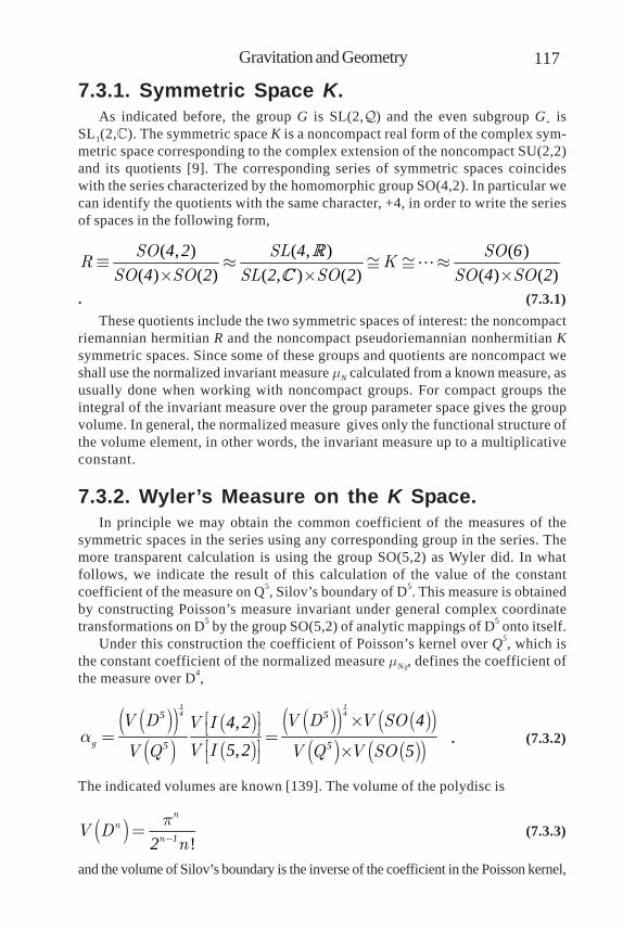
117Gravitation and Geometry
7.3.1. Symmetric Space K.As indicated before, the group G is SL(2,) and the even subgroup G+ is
SL1(2,). The symmetric space K is a noncompact real form of the complex sym-metric space corresponding to the complex extension of the noncompact SU(2,2)and its quotients [9]. The corresponding series of symmetric spaces coincideswith the series characterized by the homomorphic group SO(4,2). In particular wecan identify the quotients with the same character, +4, in order to write the seriesof spaces in the following form,
( , ) ( , ) ( )( ) ( ) ( , ) ( ) ( ) ( )SO SL SO
R KSO SO SL SO SO SO
º » @ @ »´ ´ ´4 2 4 6
4 2 2 2 4 2
. (7.3.1)These quotients include the two symmetric spaces of interest: the noncompact
riemannian hermitian R and the noncompact pseudoriemannian nonhermitian Ksymmetric spaces. Since some of these groups and quotients are noncompact weshall use the normalized invariant measure mN calculated from a known measure, asusually done when working with noncompact groups. For compact groups theintegral of the invariant measure over the group parameter space gives the groupvolume. In general, the normalized measure gives only the functional structure ofthe volume element, in other words, the invariant measure up to a multiplicativeconstant.
7.3.2. Wyler’s Measure on the K Space.In principle we may obtain the common coefficient of the measures of the
symmetric spaces in the series using any corresponding group in the series. Themore transparent calculation is using the group SO(5,2) as Wyler did. In whatfollows, we indicate the result of this calculation of the value of the constantcoefficient of the measure on Q5, Silov’s boundary of D5. This measure is obtainedby constructing Poisson’s measure invariant under general complex coordinatetransformations on D5 by the group SO(5,2) of analytic mappings of D5 onto itself.
Under this construction the coefficient of Poisson’s kernel over Q5, which isthe constant coefficient of the normalized measure mNg, defines the coefficient ofthe measure over D4,
( )( )( )
( )( )
( )( ) ( )( )( ) ( )( )
,,g
V D V D V SOV I
V IV Q V Q V SOa
é ù ´ë û= =é ù ´ë û
1 14 45 5
5 5
44 25 2 5
. (7.3.2)
The indicated volumes are known [139]. The volume of the polydisc is
( )!
nn
nV Dn
p-= 12
(7.3.3)
and the volume of Silov’s boundary is the inverse of the coefficient in the Poisson kernel,

Chapter 7 ENERGY OR MASS AND INTERACTION118
( )( )
n
n
nV Q
pG
+
=2 1
2
2 . (7.3.4)
In particular we have,
( )!
V Dp
=´
55
42 5 , (7.3.5)
( )V Qp
=3 3
5 23
. (7.3.6)
Substitution of theses expressions in equation (7.3.2) gives Wyler’s coeffi-cient of the induced invariant measure,
!g Qp
ap
æ ö÷çé ù ÷= çê ú ÷ë û ç ÷ç ´è ø
142 5
46 5 4
32 2 5
. (7.3.7)
7.3.3. Value of the Geometric Coefficient.The use of a normalized measure makes sense and is necessary on a noncompact
subspace of M. In order to calculate the coeficient of the invariant measure on thisnoncompact space we must restrict the measure mNg to this subspace by integrat-ing over a complementary compact subspace. The latter space should be thecharacteristic compact subspace of the harmonic functions on M. There is a con-tribution from the integration on this space to the value of the geometric coeffi-cient on the complementary noncompact subspace. Since mNg is defined on thecotangent space at a point *TMm and only depends on the properties of thesymmetric fiber K at m, this contribution should be independent of any solutionof the field equation. Therefore, without loss of generality we may assume spheri-cal symmetry and staticity conditions which allow a decomposition of space-timeM4 and its forms in two orthogonal subspaces, spatial compact spheres S2 and thecomplementary noncompact space-time M2 with their forms. The space M2 locallyhas the null-cone structure of a relativistic bidimesional Minkowski space.
In order to find the complete coefficient we are free to restrict the problem tothe special particular case of pure electromagnetism on a flat space-time M. Allsolutions of this restricted problem may be found as a sum of fundamental solu-tions which correspond to the Green’s function for the electromagnetic field. TheGreen’s function determines the field of a point source which always correspondsto a spherically symmetric static field relative to an observer at rest with thesource. The spherically symmetric harmonic potential solutions are determined,using Poisson’s integral formula, by its value on a boundary sphere. We see thatthe characteristic boundary space, where integration should be performed, is thesphere S2 in R3. Geometrically, in accordance with our theory, the form mNg
should

119Gravitation and Geometry
be integrated over the image of a sphere, determined by the Clifford mapping k, onthe space K. Therefore, the characteristic space is k(S2). Since S2 is compact themeasure provided by the volume element m does not require normalization. Themeasure mNg
integrated over the characteristic space gives the volume of k(S2)which is twice the volume of S2 due to the 2-1 homomorphism between standardspinors and vectors determined by its homomorphic groups SU(2) and SO(3).
Hence the complete geometric coefficient a is obtained by multiplying eq.(7.3.7), which is the value of Wyler’s coefficient calculated in the previous sec-tion, by 8p,
! . e
p p pa a
p p
æ ö æ ö÷ç ÷ç÷= = = »÷ç ç÷ ÷ç ç÷ç è ø´è ø
1 13 2 5 4 4
6 5 4 3
2 3 9 12 2 5 16 120 137 03608245
, (7.3.8)
which is equal to the experimental physical value of the alpha constant ae.
7.4. Results.We have obtained a generalized Einstein equation with geometric stress energy
tensors as the source. In vacuum, the known gravitational solutions with acosmological constant are obtained, including the Schwarzschild solution.
In general, a nonriemannian curvature scalar plays the role of variable couplingparameter. Nevertheless, in the newtonian limit, this parameter reduces to thesquare of the constant curvature parameter M (geometric energy) of the inertsubstratum solution and corresponds to the inverse of Newton’s gravitationalconstant G.
The interior Schwarzschild problem using the generalized Einstein’s equationdetermines that the Schwarzchild mass corresponds to the integral of the energydensity.
If the nonriemannian connection fields contribute to the scalar curvatureparameter in a nonnewtonian internal solution, the coupling parameter (G) wouldbe variable. This effect may be interpreted as the presence of dark matter or energy.
The only independent constant in the theory, the fine structure alpha couplingconstant, is also determined geometrically from the volume of spaces related tothe structure group.
8. Quantum Fields.We may raise the following question: Can we also obtain quantum field theory
from this geometry without recurring to classical or quantum mechanics? Thisquestion is in line with the ideal aspiration indicated by Schrödinger [140].
In quantum field theory the fields are considered operators and form an alge-bra. It appears possible that this algebra arises from geometrical properties ofsections in the principal bundle, which are properties related to group elements.Here we discuss this question, which is interesting since the group is associatedto a Clifford algebra with an anticommuting algebraic structure.
The postulates of Newton’s classical mechanics [141] are based on the con-cept of point particles and the free motion along straight lines of euclidian geom-etry. A classical field is usually seen as a mechanical system where classical me-chanics is applied. With the advent of general relativity and gauge theories, thereshould be a recognition that the geometry of the physical world is not as simple asthat provided by classical greek geometry. The idea of a physical geometry deter-mined by the evolution or flow of mass and energy [142, 143] is attractive as acriterion for setting the fundamental laws of nature.
It was natural when quantum mechanics was born [144, 145] to base its devel-opment on classical mechanics and euclidian geometry. Postulates disclosed thedifficulties with the simultaneous measurement of position and velocity of a pointparticle. Another approach, with hindsight, may be the realization that a point isnot an appropriate geometrical element on which to superpose physical postu-lates. The concepts of fields and currents are close to modern geometrical ideasand point in the direction of establishing the physical postulates on a generalgeometry, away from prejudices introduced by classical geometry and classicalmechanics.
In consequence, we developed a quantum field theory directly from physicalgeometry [56], by-passing the intermediate step of mechanics. Why should weintroduce these intermediate concepts which history of physics proved need re-vision in relativistic and quantum mechanics? Mechanics may be seen, ratherthan as a fundamental theory, as a simplification when the evolution of matter canbe approximated as the motion of a point particle.
A process of variations of the equations of the theory leads to an interpreta-tion of the varied fields as quantum operators. It is possible to define a bracketoperation which becomes the commutator for the fields associated to the connec-tion or potential and becomes the anticommutator or commutator for those asso-ciated to the frame. This bracket operation leads to the quantization relations ofquantum field theory for bosonic interaction fields and fermionic matter fields.
We show, in particular, that the theory gives quantum electrodynamics (QED)including its probabilistic interpretation. A basic feature of the geometric theoryis nonlinearity. A solution cannot be obtained by the addition of two or moresolutions and therefore it is not possible to build exact solutions from small sub-systems. Nevertheless, it is possible to study its local linearized equations which

121Quantum Fields
represent excitations which evolve approximately under the influence of statisti-cal effects inherited from the nonlinear equation.
We think of the physically related geometry as giving rise directly to fields, cur-rents and in an approximate way to both classical and quantum theories. The matterfields are represented by the frame e which is a section in a principal bundle E. Theinteraction is represented by a potential or connection w. Both the frame and theconnection are determined by the equations, in terms of an orthonormal frame u andan orthonormal set k which generates the geometric algebra A [146]. If we representparticles as excitations, then an interaction between two particles corresponds to theinteraction of two of these geometric excitations, generated by a variation. The geo-metric coupling is between the connection or potential and the matter frame.
In this chapter of the abridged presentation we shall outline various proofs. Wewill not be able to show all details of the geometric calculus of variations. For a morecomplete treatment you should see [9, 56] and the other references quoted here.
8.1. Linearization of Fields.If we introduce the bundle of connections W, a connection may be taken as a
section of this affine bundle [9, 56]. The geometrical structures of the principalfiber bundle (E,M,G) and the affine fiber bundle (W,M,w,G) are related to the alge-braic structures of their respective fibers, the frames e and the connections w.When we consider an equation relating the connection and the frame, we aredealing with Banach differentiable manifolds of sections of the fiber bundles E, Wand nonlinear differential operators which define differentiable maps betweenthese manifolds of sections. The branch of mathematics necessary for attackingthis problem is known as global nonlinear analysis [147].
We make the conjecture that the process of field quantization is the techniqueof replacing the nonlinear problem, just indicated, by a linear problem obtained byvariations of the nonlinear maps, reducing Banach differentiable manifolds ofsections to Banach linear spaces and the nonlinear differentiable maps betweenmanifolds of sections, to linear maps between Banach spaces.
From a geometrical point of view, this means working at the tangent space ofthese section manifolds at some particular “point” (section). In order to give arigorous definition to the concept of excitations we use the geometric version ofthe calculus of variations. The variation of a section leads to the geometric con-cept of the “jet” of a section. This term may physically be interpreted, in a loosemanner, as a variation or excitation of potential or matter currents.
Certain manifolds convenient to work with bundle sections are the jet bundles oforder k, indicated by JkE. They are essentially manifolds of sections equal at a point,modulus derivatives of higher order k+1 [9, 147]. Of special interest is the manifold ofsolutions g, which is the submanifold of all the sections which satisfy a given nonlin-ear differential equation. Sections obtained from a solution by the action of the struc-ture group are equivalent solutions.
If we have a variational problem, its critical sections (solutions) may be character-ized geometrically as follows: A section is critical if and only if the Euler-Lagrangeform is zero on the 1-jet prolongation [9] js of the section s,

Chapter 8 ENERGY OR MASS AND INTERACTION122
( )js
D fL h+ = 0 . (8.1.1)
The set of all the critical sections forms the differentiable manifold g of solu-tions of the variational problem. On this manifold there are vector fields whoseflow generates the space of solutions. These fields are sections of the tangentspace Tg. Instead of studying g it is possible to study the linear spaces Tgs. Wemay introduce in Tg a vector Y representing a solution of the associated variedequations. A “quantum operator” field may be related to a Jacobi field on thebundles in consideration.
Really a solution to the equations corresponds to a mapping between twosuch manifolds of solutions: one gE, corresponding to the bundle E, representinga matter frame solution and the other gW corresponding to the bundle W, repre-senting the interaction connection or potential solution.
8.2. Frame Solutions.For the manifold of frame solutions gE [56] we shall consider its tangent Tg. We
define a Jacobi vector field as a section Vs, of s*TvE, induced by the section s fromthe vertical sub-bundle of TE, such that the corresponding 1-jet prolongationsatisfies
( )jV D fL h+ = 0 . (8.2.1)
Here indicates the Lie derivative. The space of all the Jacobi vector fieldsforms the tangent space of g at a given section, denoted by Tgs. The last equationis a linearization of the nonlinear field eq. (8.1.1) which is eq.(1.2.2) in anotherform. A Jacobi field may be seen as the tangent vector to a differentiable curve ofsolutions st of the nonlinear equations at a given solution s. When we have sucha curve, we may consider it to be the integral curve of an extended Jacobi vectorfield V which takes the values Vs, at each point of the curve.
The fiber of the bundle E is the group SL(2,). The Lie algebra A of this groupis enveloped by a geometric Clifford algebra with the natural product of matricesof the orthonormal subset of the Clifford algebra. The elements of A may be ex-pressed as fourth degree polynomials in terms of the orthonormal subset of theClifford algebra.
When variations are taken, as usual, in terms of the fiber coordinates, thealgebraic properties of the fiber are not brought to full use in the theory. In orderto extract the additional information contained in the fiber which, apart from beinga manifold, is related to algebra A, we note that in many cases we have to workwith the fiber representative by the bundle homeomorphisms. We are dealing thenwith elements of G.
The vertical spaces of s*TvE are homeomorphic to the vertical spaces of TG.This means that the fiber of s*TvE is A, taken as a vector space. The association ofthe algebraic structure of A to the vertical spaces of s*TvE depends on the imageof the section s in G given by the principal bundle homeomorphisms.
When an observer frame is chosen, the local homeomorphism is fixed and the

123Quantum Fields
algebraic structure of A may be assigned to the vertical spaces. A variation of theobserver h produces an effect equivalent to a variation of the section s, andshould be taken into consideration. The total physical variation is due to a varia-tion of the section and/or a variation of the observer in the composition mappinghos, defined on a local chart U. A variation of hos is represented by a variationvector, a generalized Jacobi vector, valued in the Clifford algebra.
We are working with a double algebraic structure, one related to the algebra A,of the fiber of TE and the other to the Lie algebra of vector fields on the jetbundle JE. This allows us to assign a canonical algebraic structure to the Jacobifields, which should be defined in terms of these natural structures in each of therelated spaces.
For instance, if we use both algebraic structures and calculate the followingLie bracket of vectors,
,x ym nk ¶ k ¶é ùê úë û0 1 , (8.2.2)
where m, v are coordinates on the jet bundles and x, y the components, the resultis not a vector because of the anticommuting properties of the orthonormal set.Nevertheless, if we calculate the anticommutator, the result is a vector.
In particular, it is also known [148] that the Clifford algebra, taken as a gradedvector space, is isomorphic to the exterior algebra of the associated tangent space,which in our case is *TM. There are two canonical products, called the exteriorand the interior products, which may be defined between any two monomials inthe algebra using the Clifford product. For any element ka of the orthonormal setthe product of a monomial a of degree p by ka gives a mapping which may bedecomposed in the exterior product ka a and the interior product kaa.
Due to the associative property of the Clifford product we may extend thisdecomposition to products of monomials. We may define the grade of the productab, indicated by gr(ab), as the number of interior products in the Clifford product.The grade is equal to the number of common elements in the monomials.
For example, (k0k1) (k2k0k3) is of grade one. This decomposition may be appliedto the product of any two elements of A. It is clear that the maximum grade is thenumber of orthonormal elements and that the product of grade zero is the exteriorproduct.
The use of the exterior product instead of the Clifford product turns the alge-bra A into a Grassmann algebra isomorphic to the exterior algebra of differentialforms on the tangent spaces. This fact leads us to look for gradation of the Liealgebra structure [149].
The structure group of the theory was chosen as the simple group of innerautomorphisms of the Clifford algebra. In this sense, the group, its Lie algebra andtheir respective products arise from the Clifford algebra. In fact the Lie bracket isequal to the commutator of Clifford products. To avoid an unnecessary factor of 2we may define a Lie product as the antisymmetrized product (1/2 of the commuta-tor).
We may consider that the elements of A also satisfy the postulates to form aring, in the same manner as the complex numbers may be considered as an algebra

Chapter 8 ENERGY OR MASS AND INTERACTION124
over or as a field. In this manner, the elements of A play the role of generalizednumbers, the Clifford numbers. The candidates for the ring product are naturallythe geometric Clifford product, the exterior Grassmann product, the interior prod-uct and the Lie product. As mentioned, all these products arise from the Cliffordproduct. In fact, for any two monomials a, b Î A, all the other products a⋅b areeither zero or equal to the Clifford product ab. The geometric Clifford product ismore general and fundamental, and the others may be obtained as restrictions ofthe Clifford product. Besides, the Lie product is not associative and may needgeneralizations of the algebraic structures. On the other hand, the fiber bundle offrames, E, is a principal bundle and its vertical tangent bundle TE has for fiber aLie algebra structure inherited from the group, it would be more natural that thechosen product be closed in the algebra so that the result be also valued in the Liealgebra. For the moment, we take the more general geometric Clifford product asthe product of the ring structure of A and we shall specialize to other productswhen needed.
It is convenient, then, to work with the universal enveloping associative alge-bra of the Lie algebra of vector fields. In this manner we have an associativeproduct defined and we may represent the brackets as commutators of the ele-ments. The vertical vectors on JE may be taken as a module over the ring A. Usingthe canonical algebraic structure we may define a bracket operation on the ele-ments of the product A´. For any monomial a,b,g Î A and V,W,Z Î , define
{ } [ ], ,V W V W Za b a b g= · ´ = , (8.2.3)
turning the module into an algebra . This bracket gives the commutator oranticommutator depending on the arguments
{ } ( ) { }, ,V W W Vaba b b a= - -1 , (8.2.4)
where |ab| is the gradation of the product ab or the bracket, equal to the numberof permutations given by
( )grab a b ab= - , (8.2.5)
in terms of the degree |a| of the monomials in A and the grade of the product ab.The previous formulas are valid in general if we restrict the Clifford product to
the exterior or the interior products taking the proper number of permutations foreach case. For example in the case of Grassmann product, gr(ab) is always zero. Ifwe restrict to the Lie product, the bracket is always symmetric in eq. (8.2.3) and inthe graded Jacobi identity.
8.3. Potential Solutions.For the manifold of potential solutions gW, [56] we may proceed similarly, tak-
ing in consideration that the bundle of connections W has a different geometricalstructure than the bundle of frames E. A connection on the principal bundle maybe defined by an splitting of a short sequence of vector bundles [150]. The
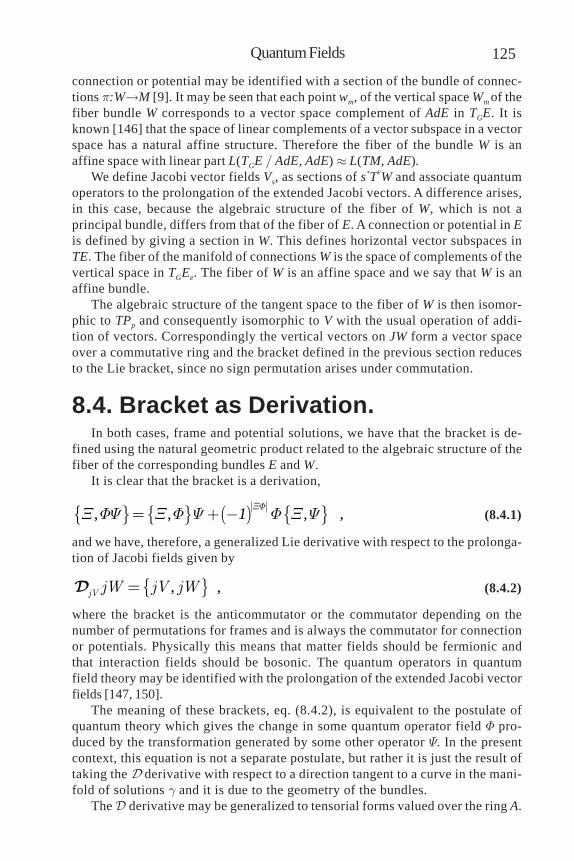
125Quantum Fields
connection or potential may be identified with a section of the bundle of connec-tions p:WM [9]. It may be seen that each point wm, of the vertical space Wm of thefiber bundle W corresponds to a vector space complement of AdE in TGE. It isknown [146] that the space of linear complements of a vector subspace in a vectorspace has a natural affine structure. Therefore the fiber of the bundle W is anaffine space with linear part L(TGE / AdE, AdE) » L(TM, AdE).
We define Jacobi vector fields Vs, as sections of s*TvW and associate quantumoperators to the prolongation of the extended Jacobi vectors. A difference arises,in this case, because the algebraic structure of the fiber of W, which is not aprincipal bundle, differs from that of the fiber of E. A connection or potential in Eis defined by giving a section in W. This defines horizontal vector subspaces inTE. The fiber of the manifold of connections W is the space of complements of thevertical space in TGEe. The fiber of W is an affine space and we say that W is anaffine bundle.
The algebraic structure of the tangent space to the fiber of W is then isomor-phic to TPp and consequently isomorphic to V with the usual operation of addi-tion of vectors. Correspondingly the vertical vectors on JW form a vector spaceover a commutative ring and the bracket defined in the previous section reducesto the Lie bracket, since no sign permutation arises under commutation.
8.4. Bracket as Derivation.In both cases, frame and potential solutions, we have that the bracket is de-
fined using the natural geometric product related to the algebraic structure of thefiber of the corresponding bundles E and W.
It is clear that the bracket is a derivation,
{ } { } ( ) { }, , ,XFX FY X F Y F X Y= + -1 , (8.4.1)
and we have, therefore, a generalized Lie derivative with respect to the prolonga-tion of Jacobi fields given by
{ },jV jW jV jW= , (8.4.2)
where the bracket is the anticommutator or the commutator depending on thenumber of permutations for frames and is always the commutator for connectionor potentials. Physically this means that matter fields should be fermionic andthat interaction fields should be bosonic. The quantum operators in quantumfield theory may be identified with the prolongation of the extended Jacobi vectorfields [147, 150].
The meaning of these brackets, eq. (8.4.2), is equivalent to the postulate ofquantum theory which gives the change in some quantum operator field F pro-duced by the transformation generated by some other operator Y. In the presentcontext, this equation is not a separate postulate, but rather it is just the result oftaking the derivative with respect to a direction tangent to a curve in the mani-fold of solutions g and it is due to the geometry of the bundles.
The derivative may be generalized to tensorial forms valued over the ring A.

Chapter 8 ENERGY OR MASS AND INTERACTION126
These derivatives represent the variation of sections along some direction in Tg,which corresponds to a generator of some transformation on the jet bundle alonga vertical direction.
The complete geometrical formulation of this physical variational problem maybe carried by constructing the extension of the vertical vector space TvEe to amodule over the ring A. In a manner similar to the complexification of a real vectorspace we consider the dual (TvEe)
* and define corresponding mappings.Thesemappings are elements of a right A-module which we designate by ATvEe. If weform the union of these spaces over the manifold E we get a fiber bundle ATvEeover E.
Further, we may construct the bundles ATvJEe over JE and s*TvE over M. Thestandard geometric version of variations may be generalized to these physicalvariations by substituting appropriately these bundles for the bundles TvE, TvJand s*TvE respectively, using the derivative and keeping track of thenoncommutative products [9, 150].
8.5. Geometric Theory of QuantumFields.
The operator bracket leads to the quantization relations of quantum field theoryusing Schwinger’s action principle. The generator of a variation F may be writtenin the jet bundle formalism by the appropriate term [9]. It may be seen that theelements entering in the expression are tensorial forms on the jet bundle whichinherit the algebraic properties of the fiber and therefore have the properties ofoperators.
The generating function F determines the variations as indicated in eq. (8.4.2).We shall write the generator F in the equivalent standard expression [151] used inquantum theory obtaining
( ) { } ( ), ,x F x dmm
s
dY Y y P dY sì üï ïï ï= = í ýï ïï ïî þ
ò , (8.5.1)
for the field operator Y variations. In this expression we recognize that the ele-ments are quantum operators, as defined above, which obey the defined bracketoperation. If we express the bracket in this relation as in eq. (8.4.1), we get
( ) ( ) ( ){ } ( ) ( ) ( ) ( ){ }, ,x x y y d y x y dm mm m
s s
dY Y P dY s P Y dY s= ò ò .
(8.5.2)It is clear that the resultant commutators for the potential operators and
anticommutators or commutators for the frame operators are none other than thequantization relations in quantum field theory for boson fields and fermion fields.
The last equation implies that

127Quantum Fields
( ) ( ){ },x yY dY = 0 , (8.5.3)
( ) ( ){ } ( ), ,x y x ym mY P d= - , (8.5.4)
where the bracket is interpreted as the commutator or anticommutator dependingon the gradation of the bracket according to the type of field.
From this formulation, the geometrical reasons for the existence of both bosonicand fermionic fields also become clear. Another advantage of this geometric for-mulation is that the operator nature of the fields may be explicitly given in terms ofthe tangent vector operators on the space of solutions and the Clifford algebramatrices.
A tangent vector may be considered as an infinitesimal action on functions ona manifold. In particular for g, the manifold of sections which are solutions, thequantum operator may be considered to act on a solution section, called thesubstratum or background section, producing solution perturbations, called quan-tum excitations. The substratum or background section takes the place of thevacuum in conventional quantum field theory.
If the manifold of sections is taken as a Hilbert manifold its tangent spaces areHilbert linear spaces. This means that the quantum operators, which act on tan-gent spaces, would act on Hilbert spaces as usually assumed in quantum theory.
If the Hilbert manifolds in question admit local harmonic sections we mayintroduce fundamental harmonic excitations. Any arbitrary excitation may be lin-early decomposed in terms of these harmonic excitations. The eqs (8.5.3, 8.5.4)determine commutation rules for the harmonic excitation amplitudes which corre-spond to the creation, annihilation and particle number operators of harmonicfield excitations at each point, with the same properties of those of the quantumharmonic oscillator. The energy of the harmonic field excitations may be definedin the usual manner leading to the concept of a quantum particle.
Nevertheless, if this geometric model is taken seriously, field (second) quanti-zation reduces to a technique for calculating field excitations or perturbations toexact solutions of theoretical geometrical equations. There may be other tech-niques for calculating these perturbations. In fact, it is known that quantum re-sults may be obtained without quantization of the electromagnetic field. See, forexample, an alternate technique to QED [152] where the self-field is taken as fun-damental.
In general relativity, the self-field reaction terms do not appear as separatefeatures in the nonlinear equations but they appear in the linearized equationsobtained using a perturbative technique. Once the geometricalnonphenomenological structure of the source term J is known, the exact equa-tions of motion for the fields describing matter, including particles, would be theconservation law for J. This relation, being an integrability condition on the fieldequations, includes all self-reaction terms of the matter on itself. There should beno worries about infinities produced by-self reaction terms. A physical systemwould be represented by matter fields and interaction fields which are solutionsto the set of simultaneous equations. When a perturbation is performed on the

Chapter 8 ENERGY OR MASS AND INTERACTION128
equations, for example to obtain linearity of the equations, the splitting of theequations into equations of different order brings in the concepts of field pro-duced by the source, force produced by the field and therefore self-reaction terms.We should not look at self-reaction as a fundamental feature but, rather, as anindication of the need to use nonlinear equations.
8.5.1. Product of Jacobi Operators in QED.The product ab in the ring A has been taken, in general, as the Clifford product
[9]. Since the fiber bundle of frames E is a principal bundle and its tangent bundleTE has for fiber a Lie algebra structure inherited from the group, it is necessarythat the chosen product be closed in the algebra so that the result be also valuedin the Lie algebra. Geometrically we should specialize the ring product, as indi-cated before, to be the Lie product. Then the product ab is zero whenever itsgradation is even. The bracket survives only when the commutator ab is nonzerobecause its gradation is odd and corresponds to the anticommutator. With thisproduct, the previouly defined bracket is the anticommutator for the matter Jacobioperator fields.
The fiber bundle of connections, W, is an affine bundle and the ring productassociated to the fiber of TW is commutative. Therefore, the bracket is the commu-tator for the connection or potential Jacobi operator fields.
As discussed before, the Jacobi vectors Vs represent fluctuations of sectionss of the fiber bundle E. The corresponding jet prolongation jV of an extension V ofVs is a vector field on JE which acts as an operator on functions on JE. A Jacobifield, as a vertical vector on the section s(M) may be considered as a displacementof s. Similarly, its jet prolongation may be considered as a displacement of js, inother words a variation,
( )j
jj
d sV s
dl= . (8.5.5)
This linear action of the Jacobi fields on the substratum sections allow us toassociate them with quantum theory objects. We may consider the inert substra-tum section as the vacuum state |0ñ of the physical system and the Jacobi fields asphysical linear operators Y which have a natural geometric action on the states.
A given physical matter section may be expressed in terms of reference framesections. This reference frames are also physical systems. Hence they may evolveunder the action of the same group that acts on the matter sections. This repre-sents the known equivalence of the active and passive views of evolution. Wemay consider the physical system evolving in a fixed frame or, equivalently, wemay consider the system fixed in an evolving reference frame.
We may choose the reference frame so that the substratum section does notevolve. In this condition the substratum section remains fixed and the Jacobioperators obey the first order linearized equations of motion. (Heisenberg pic-ture).
The Jacobi vector fields and their jet prolongations transform under the ad-
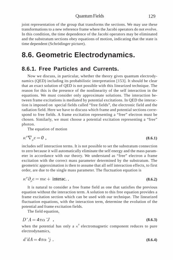
129Quantum Fields
joint representation of the group that transforms the sections. We may use thesetransformations to a new reference frame where the Jacobi operators do not evolve.In this condition, the time dependence of the Jacobi operators may be eliminatedand the substratum sections obey equations of motion, indicating that the state istime dependent (Schrödinger picture).
8.6. Geometric Electrodynamics.
8.6.1. Free Particles and Currents.Now we discuss, in particular, whether the theory gives quantum electrody-
namics (QED) including its probabilistic interpretation [153]. It should be clearthat an exact solution of QED is not possible with this linearized technique. Thereason for this is the presence of the nonlinearity of the self interaction in theequations. We must consider only approximate solutions. The interaction be-tween frame excitations is mediated by potential excitations. In QED the interac-tion is imposed on special fields called “free fields”, the electronic field and theradiation field. Here we have to discuss which frame and potential sections corre-spond to free fields. A frame excitation representing a “free” electron must bechosen. Similarly, we must choose a potential excitation representing a “free”photon.
The equation of motion
emmk = 0 , (8.6.1)
includes self interaction terms. It is not possible to set the substratum connectionto zero because it will automatically eliminate the self energy and the mass param-eter in accordance with our theory. We understand as “free” electron a frameexcitation with the correct mass parameter determined by the substratum. Thegeometric approximation is then to assume that all self interaction effects, to firstorder, are due to the single mass parameter. The fluctuation equation is
interac.e memmk ¶ = + . (8.6.2)
It is natural to consider a free frame field as one that satisfies the previousequation without the interaction term. A solution to this free equation provides aframe excitation section which can be used with our technique. The linearizedfluctuation equations, with the interaction term, determine the evolution of thepotential and frame excitation fields.
The field equation,
D A Jpa* *= 4 , (8.6.3)when the potential has only a k0 electromagnetic component reduces to pureelectrodynamics,
d dA jpa* *= 4 . (8.6.4)

Chapter 8 ENERGY OR MASS AND INTERACTION130
It is natural to consider a free potential field as one that satisfies the previousequation with j=0. A solution to the field equation provides a substratum poten-tial section which can be used with the proposed technique.
In order to get the standard QED from the geometric theory, we have to reducethe structure group to one of the 3 U(1) subgroups in the SU(2) electromagneticsector. The corresponding u(1) component of the fluctuation of the generalizedconnection is the electromagnetic potential Am. Similarly, an electromagnetic fluc-tuation of the matter section determines a fluctuation of the generalized current.This fluctuation must be generated by one of the three electromagnetic genera-tors, for example k5. The standard QED electric current is the electromagneticsector component of this current fluctuation,
( ) ( )( ) ( )
tr tr ,
tr tr
j J J
J J
d k k k d k k k k
k k k k k
é ù= = ê úë û
= =
1 2 3 1 2 3 51 1 14 4 2
5 1 2 3 01 14 4 . (8.6.5)
It was already shown that the standard electric current in quantum theory isrelated to the k0 component of the generalized current,
( )tr trJ e em m mk k k Yg Y= =0 01 14 4 , (8.6.6 )
which is the electric current for a particle with a charge equal to one quantum inthe geometric units.
8.6.2. The Interaction Hamiltonian.We may choose a reference frame so that both substratum sections, which
include the corresponding self interactions of the two “free” systems, also in-clude an observer dependent free motion for the two excitations. The two substra-tum sections are not solutions to the interacting system, they are free backgroundsolutions. This situation corresponds to an interaction picture in QED. By choos-ing an appropriate reference frame, the substratum sections (states) have the“free motion”, including self interaction effects and the excitation Jacobi opera-tors represent the dynamics of the interaction of the two systems, excluding thefree self interactions.
The only invariant effect of the self interaction in the free motion of the fieldsis the mass parameter m. The remaining effects of the total physical interaction,associated with the fluctuation fields, correspond to an effective net interactionenergy which may be written as
e eA mI Hmmk - = . (8.6.7)
The first part of H is the total physical interaction. The meaning of the secondpart is that massive self energy is not included in the fluctuation and this method(or QED), by construction, is not adequate for a calculation of bare mass.
It is known that the lagrangian for the first variation of the Lagrange equationsis the second variation of the lagrangian. For both free fields, the corresponding

131Quantum Fields
second variation of the lagrangian gives the free Maxwell-Dirac field lagrangian.Since the current variation has only a k0 component given by eq.(8.6.6 ) and thepotential variation has Am for k0 component, the second variation or interactionhamiltonian gives, in terms of these interaction field Jacobi operators dG, dJ,
( ) ( )tr trH L A J A Am mm md d d k k Yg Y Yg Yº = = = -2 0 01 1
4 4 , (8.6.8)
which is the standard interaction hamiltonian in QED.We have obtained a framework of linear operators (the prolongations of Jacobi
fields) acting on sections forming a Banach space (states) where the operatorsobey the bracket commutation relations, commutators for A and anticommutatorsfor Y. Furthermore, the geometric lagrangian of the theory reduces to a lagrangianin terms of operators which is the standard lagrangian for QED.
From this point we can proceed using the standard techniques, language andnotation of QED, equivalent to the geometric techniques, for any calculation wewish to carry in this approximation of the geometric theory. The result of thecalculation should be interpreted physically, in accordance with the geometricideas. This is our next task, to obtain a statistical interpretation to fluctuations inthe geometrical theory.
8.6.3. Statistical Interpretation.The physical significance of the local sections in the nonlinear geometrical
theory includes the holistic influence of the total universe of matter and interac-tions. The geometry of the theory, including the notion of excitations, is deter-mined by all sources in the universe. Within this geometric theory and its interpre-tation, it is not appropriate to consider the sections to be associated with a singleparticle or excitation. Rather, they are associated to the global nonlinear geometriceffects of bulk matter and radiation.
This is not the customary situation in which physical theories are set. It isusual to postulate fundamental laws between elementary microscopic objects (par-ticles). In order to translate the global universal geometry to the usual micro-scopic physics, since we associate particles to geometric excitations, we shallestablish what we call a “many excitations microscopic regime”, distinguishedfrom the situation described in the previous paragraph.
Statistics enter in our approach in a manner different than the usual one, wherefundamental microscopic physical laws are postulated between idealized elemen-tary particles and statistical analysis enters because of the difficulties that arisewhen combining particles to form complex systems. Here, the fundamental lawsare postulated geometrically among all matter and radiation in the system (thephysical universe) and statistical analysis arises because of the difficulties andapproximations in splitting the nonlinear system into elementary microscopic lin-ear fluctuation subsystems. As a consequence of this holistic situation, the re-sults associated to fundamental excitations must have a natural (classical) statis-tical character corresponding to that of quantum theory.
We consider that we may work in two different regimes of the physicalgeometric theory. One is the holistic global geometric holophysical regime
Chapter 8 ENERGY OR MASS AND INTERACTION132
which does not represent particles, where there are exact nonlinear equationsbetween the local frame sections, representing matter, and a potential sectionrepresenting the interaction. The other is the many-excitations microscopic re-gime where we have linearized approximate equations between the variations ofthe frame and potential sections, representing particles and fields.
In the many-excitations regime, the nonlinear local effects of the interactionremain hidden in a substratum solution and are replaced by linear approximatelocal effects among the subsystems, seen as a collection of excitations on thesubstratum. The number of excitations is naturally very large and the cross inter-actions among them preclude an exact treatment for a single excitation. Instead itis necessary to treat the excitations as one among a large ensemble and use clas-sical statistical theory.
The geometric excitations form statistical ensembles of population density ni.It is not possible to follow the evolution of any single one because of the previ-ous arguments. It is absolutely necessary to use statistics in describing the evo-lution of the excitations. The situation is similar to that of chemical reactions orradiation, where atoms or particles are statistically created or annihilated.
There are adequate classical statistical techniques for describing these pro-cesses. The mathematical methods used in physical chemistry may be applied tothe geometric excitations. In particular we may use the theory of irreversible ther-modynamics [154] to calculate the rates of reaction between different geometricexcitations. The process is described by the flux density characterizing the flowof n excitations between two systems or reaction rate.
It is also necessary to introduce a driving force function , which is calledaffinity and represents differences of thermodynamic intensive parameters. Theuse of these classical concepts is derived from fundamental statistical analysis. Incase of equilibrium between two different subsystems, both the affinity and theflux are zero.
The identification of the affinity is done by considering the rate of productionof entropy s. The affinity associated to any given excitation is given in terms isthe energy u, the temperature T and is the excitation potential m, similar to thechemical potential used to determine the statistics of chemical reactions.
The statistical flux is a function of the affinity and we see that the statistics ofreaction of geometric excitations should depend on the classical geometric en-ergy of the excitations. An excitation is an extensive parameter x which has asso-ciated an intensive parameter F thermodynamically related with the change ofenergy. At a point, the excitation is a function of time which may always be decom-posed in harmonic functions. In general, the energy of harmonic oscillations de-pends on the excitation amplitude. Thus, the probability of occurrence of a singlereaction event, implicit in the reaction rate determined by the excitation potential,depends on the excitation amplitude. This is the significance of the probabilisticinterpretation of quantum fields.
In some cases, for linear markoffian systems (systems whose future is deter-mined by their present and not their past), the flux is proportional to the affinityand the calculation of reaction rates is simplified, indicating explicitly the depen-dence of the flux on the difference of excitation potentials.

133Quantum Fields
The radiation excitation must be a massless, long range, geometric connectionpotential which is a representation of the group G=SL(2,) induced from thesubgroup P=Sp(2,). As indicated in section 2.1, this representation is character-ized by the quantum number helicity determined by a representation of the isot-ropy subgroup SO(2,1). The corresponding fundamental irreducible representa-tion, which is the photon, must carry a quantum of angular momentum. The pres-ence of helicity means that a photon is a harmonic oscillation of some frequencyn. Then the Jacobi vector operator Y may be decomposed in its irreducible pho-tons using a Fourier series decomposition.
It should be clear that the geometric commutation or anticommutation rela-tions of the Jacobi vector operators Y imply similar relations for the fundamentaloscillator amplitudes (Fourier components) a. Consequently the energy of thesegeometric oscillators is quantized, with the same results of the quantum theory.These amplitudes become creation or annihilation operators a. Under these con-ditions the number operator,
†N a a= , (8.6.9)has discrete eigenvalues n which indicate the number of photons and determinethe energy of the oscillators. The energy quanta are the eigenvalues
ne næ ö÷ç= + ÷ç ÷çè ø
12
, (8.6.10)
in geometric units where Planck’s constant equals 1.The energy of the excita-tions has quanta of value equal to the frequency n.
In order to illustrate this statistical character of the linearized regime, we dis-cussed [9] the wave corpuscular duality of light and matter within the concepts ofthe geometric theory. There are excitations which correspond to multiple particlesand lead to Schrödinger’s “entangled states”, typically demonstrated in Young’sdouble interference experiment as shown in figure 7. In the last decades there hasbeen a revolution in the experimental preparation of multiparticle entanglements[155, 156, 157, 158, 159]. There are no exact equations for physical situations with
Figure 7Young’s doubleinterferometer.
yz x
A
B
B’
A’
PP’ d/2
-d/2

Chapter 8 ENERGY OR MASS AND INTERACTION134
a single excitation. The outcome of microscopic transition experiments dependson the excitation potentials of the systems. Any real physical situation in themicroscopic linear regime of the theory requires the use of statistics for the totalsystem.
A physical particle (f.e. a photon) is an excitation of the corresponding sub-stratum field. In geometric terms, a Jacobi vector Y, associated to a variation of asection e or w, represents the particle. As indicated in the previous section, it isnot possible to follow the evolution of a single excitation Y. The classical statisti-cal approach is to treat the radiation as a thermodynamic reservoir of excitations.This approach was used in blackbody radiation[160, 161, 162] and was the originof Planck’s quantum theory.
The amplitude of the Jacobi excitation, which is a product representation ofthe two excitations, is
( ) ( )cos cosd
d
adx x y x z
dpq pq
Yl l
+
-
é ù é ùê ú ê úµ + +ê ú ê úë û ë û
ò2
2
. (8.6.11)
If d is much smaller than l/q the integral gives the product of two Young’spatterns as it should. If, on the contrary, d is much larger than l/q, this integralgives,
( )cosaz y
pqY
læ ö÷çµ - ÷ç ÷çè ø2 . (8.6.12)
and the excitation potential, which gives the probability for the simultaneousdetection of particles at P and P’, is
cos z y
2
. (8.6.13)
There are regions of high and low probabilities because of the interference of theexcitation amplitudes.
In recent years, similar ideas lead to introduction of stochastic quantization[163, 164], which has been shown to be equivalent to path integral quantization.Our approach is different, for example we do not introduce evolution along afictitious time direction as done in stochastic quantization. We rely on the exist-ence of a global nonlinear geometry which makes a practical necessity the statis-tical treatment of the linearized equations describing the evolution of microscopicsubsystems.
The requirement of statistics necessarily leads to the probability interpreta-tion of quantum theory. If, within a particular experimental setup, we can physi-cally distinguish between two excitation states, there is no room to apply statis-tics and there follows the absence of the interference pattern. This is the contentof Feynman’s statement about experimentally indistinguishable alternatives [165].Fundamentally the quantum statistics are the classical statistics of section excita-
135Quantum Fields
tions in this physical geometry. The objections raised by Einstein [166, 167] to theprobabilistic interpretation are resolved automatically because these statisticsenter due to the lack of detailed knowledge of the states of many excitations.
8.7. Results.The process of field quantization is the technique of replacing the nonlinear
geometric problem by a linear problem obtained by variations of the nonlinear maps.The properties of the linear variations determine a bracket operation which becomesthe commutator for the varied potential fields and also becomes the anticommutatoror commutator for the varied matter fields. This bracket operation leads the quantizationrelations of quantum field theory for bosonic interaction field and fermionic matterfields. The substratum plays the role of the quantum vacuum.
Quantum electrodynamics is obtained in the corresponding limit. The nonlineargeometric equations apply to the total universe of matter and radiation. If we workwith excitations, this implies the need to use statistical theory when considering theevolution of microscopic subsystems. Use of classical statistics, in particulartechniques of irreversible thermodynamics, determines that the probability ofabsorption or emission of a geometric excitation is a function of the classical energydensity. Emission and absorption of geometric excitations imply discrete changes ofcertain physical variables, but with a probability determined by its wave energy density.The geometric properties of the excitations are the germ of quantum physics.
Quantum Field Theory (QFT) should be used to calculate the perturbation correc-tions to the geometric bare values of the microscopic physical magnitudes. In thismanner the proper results of particular experiments are determined. As an example,higher order corrections for the magnetic moments were calculated in section 5.2.

Appendix
Introduce the real anticommuting matrices,
ré ùê ú= ê úë û
0 11 0
, (A.1)
sé ùê ú= ê ú-ë û
1 00 1
. (A.2)
These anticommuting elements form an orthonormal subset designated by
{ },ir r s= (A.3)
and generate two additional matrices,
eé ùê ú= ê ú-ë û
0 11 0
, (A.4)
Ié ùê ú= ê úë û
1 00 1
. (A.5)
These matrices form the nonommutative ring of 2-dimensional real matrices,which is the Cl(2,0) Clifford algebra or R2,0 . These matrices are similar to thequaternions but they are not isomorphic algebras. Nevertheless, their evenparts are isomorphic and may be identified with the complex numbers . Becauseof the similarit ies we shall designate this nondivision ring as thepseudoquaternions ,
[ ] [ ]Ir s e r r r r r r= 1 2 1 2 1 1 . (A.6)
The generators E of the Cl(3,1) algebra or R3,1, designated as A, may beexpressed as 2´2 matrices over the ring. The orthonormal subset km generatesthe rest of the base. Explicitly in this representation the odd sector of the algebraA including the orthonormal subset is, up to equivalence under automorphisms,
, r
k k k k k kr
é ùê úê úé ùê úê ú= = =ê úê ú- -ë û ê úê ú-ë û
0 5 0 1 2 3
0 0 0 10 0 0 1 0
0 0 1 0 01 0 0 0
, (A.7)

137Appendix
, 0 r
k k k k k kr
é ù-ê úê úé ù- -ê úê ú= = =ê úê úë û ê úê úë û
1 5 1 0 2 3
0 1 0 00 1 0 0 0
0 0 0 10 0 1 0
, (A.8)
, s
k k k k k ks
é ùê úê úé ù -ê úê ú= = =ê úê úë û ê úê ú-ë û
2 5 2 0 3 1
1 0 0 00 0 1 0 0
0 0 0 1 00 0 0 1
, (A.9)
, r
k k k k k kr
é ùê úê úé ùê úê ú= = =ê úê úë û ê úê úë û
3 5 3 0 1 2
0 0 0 10 0 0 1 0
0 0 1 0 01 0 0 0
. (A.10)
The even sector of the algebra A is, up to equivalence under automorphisms,
I
Ik k s
é ùê úê ú é ùê ú ê ú= = =ê ú ê úë ûê úê úë û
0 1 1
0 0 1 00 0 0 1 01 0 0 0 00 1 0 0
, (A.11)
ek k s
e
é ù-ê úê ú é ù-ê ú ê ú= = =ê ú ê úë ûê úê ú-ë û
0 2 2
0 0 0 10 0 1 0 00 1 0 0 01 0 0 0
, (A.12)
I
Ik k s
é ùê úê ú é ùê ú ê ú= = =ê ú ê ú- -ë ûê úê ú-ë û
0 3 3
1 0 0 00 1 0 0 00 0 1 0 00 0 0 1
, (A.13)

Appendix ENERGY OR MASS AND INTERACTION138
ie
k k se
é ùê úê ú é ù-ê ú ê ú= = =ê ú ê ú- -ë ûê úê úë û
1 2 3
0 1 0 01 0 0 0 00 0 0 1 00 0 1 0
, (A.14)
ie
k k se
é ùê úê ú é ù-ê ú ê ú= = =ê ú ê úë ûê úê ú-ë û
2 3 1
0 0 0 10 0 1 0 00 1 0 0 01 0 0 0
, (A.15)
Ii
Ik k s
é ùê úê ú é ùê ú ê ú= = =ê ú ê ú- -ë ûê úê ú-ë û
3 1 2
0 0 1 00 0 0 1 01 0 0 0 00 1 0 0
, (A.16)
Ii
I
ek k k k k
e
é ùê úê ú é ù é ù-ê ú ê ú ê ú= = = ºê ú ê ú ê úë û ë ûê úê ú-ë û
0 1 2 3 5
0 1 0 01 0 0 0 0 00 0 0 1 0 00 0 1 0
. (A.17)
For any element a of the algebra A, the conjugate anti-involution is
† †a ak k= 0 0 (A.18)
which corresponds to Dirac’s conjugation. The antiinvolution † is the transpose ofthe real 4 x 4 matrices. The main involution,
†a ak k= 5 5 , (A.19)
induces a direct sum decomposition of A into its even subalgebra A+ and thecomplementary odd part A-. Associated to the eigenvalues of the main involution,we may introduce a quantum number called rarity r, defined by the eigenvalues ofthe odd projection operator,
( ) ˆrar a aa -=
2 . (A.20)
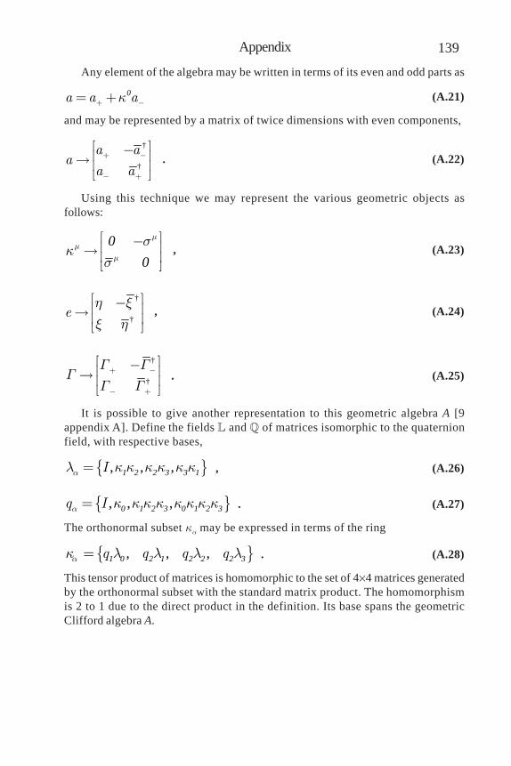
139Appendix
Any element of the algebra may be written in terms of its even and odd parts as
a a ak+ -= + 0 (A.21)
and may be represented by a matrix of twice dimensions with even components,
†
†
a aa
a a+ -
- +
é ù-ê ú ê úë û
. (A.22)
Using this technique we may represent the various geometric objects asfollows:
mm
m
sk
s
é ù-ê ú ê úë û
00
, (A.23)
†
†eh xx h
é ù-ê ú ê úë û
, (A.24)
†
†
G GG
G G+ -
- +
é ù-ê ú ê úë û
. (A.25)
It is possible to give another representation to this geometric algebra A [9appendix A]. Define the fields and of matrices isomorphic to the quaternionfield, with respective bases,
{ }, , ,Ial k k k k k k= 1 2 2 3 3 1 , (A.26)
{ }, , ,q Ia k k k k k k k k= 0 1 2 3 0 1 2 3 . (A.27)
The orthonormal subset ka may be expressed in terms of the ring
{ }, , ,q q q qak l l l l= 1 0 2 1 2 2 2 3 . (A.28)
This tensor product of matrices is homomorphic to the set of 44 matrices generatedby the orthonormal subset with the standard matrix product. The homomorphismis 2 to 1 due to the direct product in the definition. Its base spans the geometricClifford algebra A.
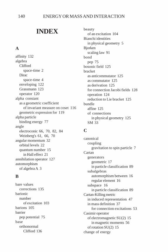
ENERGY OR MASS AND INTERACTION140
INDEX
Aaffinity 132algebra
Cliffordspace-time 2
Diracspace-time 4
enveloping 122Grassmann 123operator 120
alpha constantas a geometric coefficient
of invariant measure on coset 116geometric expression for 119
alpha particlebinding energy 77
angleelectroconic 66, 70, 82, 84Weinberg's 61, 66, 70
angular momentum 32orbital levels 22quantum number 15
in Hall effect 21annihilation operator 127automorphism
of algebra A 3
B
bare valuescorrections 135
barionicnumber
of excitation 103barions 105barrier
pep potential 75base
orthonormalClifford 136
beautyof an excitation 104
Bianchi identitiesin physical geometry 5
Bjorkenscaling law 91
bondpep 75
bosonic field 125bracket
as anticommutator 125as commutator 125as derivation 125for connection Jacobi fields 128operation 124reduction to Lie bracket 125
bundleaffine 125of connections
in physical geometry 125SM 33
C
canonicalcoupling
gravitation to spin particle 7Cartan
generatorsgeometric 17in particle classification 89
subalgebrasautomorphism between 16regular element 16
subspace 16in particle classification 89
Cartan-Killing metricin induced representation 47in mass definition 37
for connection excitations 53Casimir operator
of electromagnetic SU(2) 15in magnetic moments 56
of rotation SU(2) 15change of energy

141Index
as intensive parameter 132charge
electricopposite signs 20
measurement of 33quantum
in Hall effect 21index in Hall effect 25measurement 34
quantum number 15charm
of an excitation 104classification
of connections 87group G 88group L 88group P 88
of interactions 92of matter excitations 92
colorof an excitation 107
commutation relationHeisenberg 41quantum field theory 127
comoving reference frame 9complex
structure 50conductivity
fractionsFQHE 26
conjugationcharge 18, 89
connectionclassification 87cosmic background 37even part 139in physical principle 5odd part 139substratum 48total 37
connection field 125excitations
equation for 54mass for 53
free 129connection fields
excitationsin a lattice 62
conservation equation 7constant
coupling 6identification 34
electron charge 34fine structure alpha 34gravitational
determined by substratum 114weak interactions 85
coordinatecomoving 9
correctionsto bare values 135
cosetC
in mass ratios 50volume of 50
complex structurein mass ratios 50
in structure group G 117in mass ratios 46
K 117equivalence relation in 50
symmetricin structure group 46
volume of 50Coulomb's law 35coupling
canonicalgravitation to spin particle 7
creation operator 127critical sections 121current
canonical 29conservation 7electric 130interaction 81source 6
geometric 116curvature

ENERGY OR MASS AND INTERACTION142
in physical geometry 5Maxwell 12Riemann 12
D
De Sitter space 15derivative
Lie 122deuteron
binding energy 75model 71
Diracalgebra 4equation
2-component form 39general form 36
generalized equation 4, 7explicit mass term 39
spinor 40driving force function 132duality
of representations 18, 90
E
Ehrenfest’s theorem 41eigenvalue
mass 43Einstein
equation 13, 110Einstein equation 111electric charge
quantum 34quantum number 21
electric current 130electrocone
angle 66, 82, 84quantum subspace
in electromagnetic su(2) 57electrodynamics
classical 12quantum 129
electromagnetismgenerator
quantization 55generators 32Maxwell's equations 12standard 11vector potential 38
in Pauli's equation 65magnetic moments 57, 66
electron 91as unit of charge 34charge
negative 20roles of 34
fieldfree 129
magnetic momentradiative corrections 68
mass 52energy
bindingalpha particle 77deuteron 75
dark 111, 115equipartition 10, 47field 8fundamental 6magnetic
of excitation 66energy level
degenerateof orbiting electron 24
degenerate superfluxedpossible quanta 24
firstmagnetization flux quanta 23net flux quanta 23of orbiting electron 23
Landau 22energy momentum
equationand gravitation 109
energy momentum tensordue to torsion 111from coset fields 110matter current 110

143Index
energy operator 41energy potential 5entangled states
Schrödinger 133enveloping algebra
of vector fields 124equation
Dirac2-component form 39generalized 4, 7
Einstein 111energy momentum
and gravitation 109Helmholtz 61Mathieu
deuteron 73Maxwell 12Pauli
at nuclear distances 70generalized equation 65
Stehphenson-Yang 112Yang 13Yukawa 54
equation of motionand conservation equation 8with explicit mass 11, 38
nonrelativistic approximation 64equipartition
energy 10, 47equivalence
relationin coset K 50under relativity boosts 48
relativistic relationapplication 51
evolutionactive view 128passive view 128
excitationas extensive parameter 132connection
mass 45point 30potential 132
for Young's experiment 134representation 43topological 94
expectation value 31of charge 33
experimental flux quanta 21experimental values
and bare values 135extensive parameter 132external space 43
F
familieslepton 95particle 94
Fermicurrent
for weak interactions 83lagrangian
for weak interactions 82theory
lagrangian and current 85fermionic field 125field
bosonic 127fermionic 127
field energy 8field equation 5field quantization 120flavor
of an excitation 103, 107flux
quantum 18flux density
of excitations 132fractional quantization 21frame
as set of states 30classification 92composite
of interacting systems 80eigenvector 30even part of 139matter

ENERGY OR MASS AND INTERACTION144
current 7odd part of 139reference
in jet bundle 128frame excitations
as group representations 14as particles 14
frame sectionsas wavefunctions 32
free connection field 129free matter frame 129free particle field 129function
Green'sfor connection excitations 54from fluctuation equation 84in weak interactions 83
functionalDirac 30
G
Gell-Mann-Nakano-Nishijima formula104
generatoras quantum operator 32electromagnetic 32
quantization 55rotation 32
geometricelectrodynamics 129
geometric algebraA(3,1) 3
Clifford 2algebra A
decomposition 139Clifford product
grade of 123exterior product 123interior product 123Lie product 123
geometric currentassociated to geometric measure
in coset K 116associated with excitations 29
of a matter excitationgeneral form 30
geometric excitationannihilation operator 127creation operator 127equation for connection 54G-particle
compared with P-particle 20defines positive charge 20quantum numbers 18
L-particlequantum numbers 20
number operator 127P-particle
negative charge 20quantum numbers 19, 20
point 30representation on symmetric space 43
geometric groupG 14subgroup L (Lorentz) 14subgroup of electromagnetism 15subgroup of rotations 15subgroup P 14
geometric measurementas functional 30result of 31
geometric spin 31geometric structure
triple 65, 91, 96geometric unit
of charge 34of mass 85
geometric valuesand experimental values 135
geometrical regime 132geometrical theory 8geometry
as germ of quantum physics 28physical 1
global nonlinear analysis 121gradation
of product 124gravitation
145Index
constantdetermined by substratum 114
Einsteinequation 13, 110
energy momentum tensorgeometric 13, 111, 119
newtonian limit 112and the substratum 114
torsion 111Yang's theory 13
groupDe Sitter 14G 14geometric 14ISO(3,1) 16L 14Lorentz 1, 14P 14Poincaré 16SL(2,C) 1, 14SL(2,Q)
homotopy group of 94physical significance 3subgroups 14
SL(4,R) 2and topological numbers 94
SO(3,2) 14SO(4) 15structure 1SU(2) 14
and electric charge 32and electromagnetism 11rotation 31
SU(3)xSU(2)xU(1) 107U(1)
electromagnetism 1group action
on itself 43
H
Hall conductivityand FQHE 25
Hall effectcarrier model
magnetic vortex 25conductivity 25
fractional values 26plateaus 27
half levelpopulation 25
Landau levelfilling condition 25
vortex modellinked flux 25
hamiltonianinteraction 131
Heisenberg commutation relation 41helicity 16
photon 133Helmholtz
equation 61hermiticity
degree of non 84holonomy
group 64homotopy
product 95hyperbolic manifold
substratum 10hypercharge
strongof an excitation 104
weakof an excitation 104
I
identitiesBianchi
in physical geometry 5inclusion
mapping 2induced representation 44
as sections of vector bundle 14Cartan-Killing metric
in mass ratios 47induced from subgroup 14
of G 15inert substratum 10, 48, 49, 128

ENERGY OR MASS AND INTERACTION146
integrability condition 6intensive parameter 132interaction
classificationG/P generators as strong nuclear92L-connection as gravitation 92P/L generators as electroweak 92
interaction connection solution 122interaction current 81
in standard quantum notation 83interaction energy
net 130interactions
electromagnetic 12gravitational 13, 110
geometric 111in physical geometry 13
strong 92interference experiment
Young's double 133internal space 43invariant measure
normalized 117irreducible representation
fundamental 18isotopic spin
of an excitation 104
J
Jacobifields
canonical algebraic structure 123double algebraic structure 123
operatorevolving 128fixed 129interaction effects 130
vector fieldon connection solutions 125on frame solutions 122
jet bundlein physical geometry 121
jet prolongation 121
K
kaon 100Killing vector 10
L
lagrangianfor first varied equation 82
lawCoulomb 35
left handed componentof spinor 41
leptonas topological excitation 94families 95masses 96. See mass values
general expression 97masked 99muon 98tau 98
leptonic numberof an excitation 103
Liederivative 122
generalized 125limit
newtonianand the substratum 114in physical geometry 112
linearization 121, 135first varied equation 82
long range fieldselectromagnetic
and magnetic moment 66Lorentz
equation of motion 8
M
magnetic fieldmotion in constant field 22
magnetic fluxbare flux
quantum number 23

147Index
enclosed by loop 23magnetization
quanta 23net flux
possible quanta in level 24quantum number 23
orbital quanta 23discrete change in 24
quantum 18quantum number 21
magnetic moment 66anomalous increase 67electron 68neutron 69proton 69
manifoldHilbert
in physical geometry 127hyperbolic
substratum 10of sections 121of solutions 121
many excitations regime 132map
inclusion 2non linear differentiable 121
markoffian system 132mass
as parameter in Dirac's equationand the substratum 38for different representations 37for particles 45
bare 46corrections to 46in Dirac's equation 38in general 29in induced representation 49of G-excitations 49of H-excitations 49
concept of mass 6, 35connection excitations 45definition 37excess
neutron 77
in the induced representation 114of leptons 96
general expression 97parameter 35
constant 38in QED 130
Schwarzschild 114mass eigenvalue 43mass values
eta 101heavy leptons
muon/electron 98tau/electron 98
kaon/pion 100masked 99pion/muón 99stable particles
electron/proton 52neutrino/proton 52
weak bosons 61Mathieu
equationfor deuteron 73
functionshyperbolic radial 74
matterclassification 92dark 111, 115
matter field 125matter frame
as set of states 30Clifford structure of 32current 7eigenvector 30free 129solution 122
matter state 8Maxwell curvature 12measurement
current subject of 29mathematical representation 30physical 28
mesons 105metric

ENERGY OR MASS AND INTERACTION148
Cartan-Killingin mass ratios 45
space-timegravitational 110in newtonian limit 112
modelBarut's 103deuteron 71neutron 76
moduleover ring A 124
momentmagnetic
in physical geometry 66momentum
angular 32canonical 23conjugate 29kinetic 23operator 41
and geometric Casimir operator 44in physical geometry 43
momentum spacegeneralized 43
multiplicative relationamong quantum numbers 18
muonmass
as topological excitation 98
N
neutrinoas perturbation of composite frame 81association with even part of electron
in weak interactions 81equation 40in weak interactions 80mass 52properties 91
neutron 69mass excess 77model 76
Newtongravitation 112
newtonianlimit
and the substratum 114in physical geometry 112
O
observable 29observer
complete 3standard space-time 4
operationbracket 124
operatorCasimir 44
electromagnetic SU(2) 56LaPlace-Beltrami 44momentum 43quantum
bosonic 127fermionic 127
orientationentanglement 2
orthonormalsubset
in physical geometry 7
P
particle3-point
as proton 91alpha
binding energy 77families 94field
free 129number operator 127weak boson 61
particlesBarut's model 103geometric classification
families 94G-frame as hadronic matter 92L-frame as neutral matter 92
149Index
P-frame as leptonic matter 92leptons 98masses 98, 99, 100mesons 100properties
charge 89flux 89magnetic moments 66masses. See mass valuesmoments. See magnetic momentspin 89wrapping 94
stableelectron 91neutrino 91proton 92
Pauli’s equationgeneralized 65
at nuclear distances 70pep
bond 75potential barrier 75
perturbationof substratum 81
perturbation correctionsto bare values 135
physical geometryand electromagnetic charge 14and gravitation 109and measurements 28and particles 87and quantum field theory 120
pictureHeisenberg 128interaction 130Schrödinger 129
pion 99Poincaré
group 16polydisc
unitvolume of 117
potential 5, 37and substratum curvature 11, 113
dynamicdue to matter 37
for the substratum 10of substratum 37
in mass definition 48strong
magnetic 64potential barrier
pep 75principle
of relativitygeneralized 3
Schwinger's action 126uncertainty
Heisenberg's 41probabilistic interpretation 132
in Young's interference experiment134
productconvolution 37
in mass ratios 47Lie
in QED 128proton 92
chargedefined 20
magnetic momentcorrections 69
mass 52quark structure 90
3-point particle 91pseudoquaternion 136
Q
quantumfundamental
angular momentum 18magnetic flux 18
quantum electrodynamics 120, 129standard techniques 131
quantum field theory 120variational principle 126
quantum mechanicscomplex structure of 32

ENERGY OR MASS AND INTERACTION150
of free particles 39quantum numbers
algebraic 89topological 94
quantum of flux 21quantum operator 122
change in 125quark
as dual representation of G 90as geometric excitation 91, 102as leptonic excitation 102flavor 102
quarkoniumconjecture 105
quaternion 139pseudo 136
R
radiationfield
free 129range
longmagnetic field 65
rarityof an excitation 104operator
as odd projector 138reaction
self field 127reference frame
comoving 9in jet bundle 128
regimegeometrical holophysical 132microscopic excitation 132
regular elementas spin and charge generators 17
relationcommutation or anticommutation 127
relativity of interactions 12representation
dual 90dual fundamental of group G
as quarks 90fundamental 89fundamental of G
as proton 90fundamental of L 20
as neutrino 90fundamental of P 19
as electron 90resistivity
fractionsFQHE 26
Riemanncurvature form 12tensor 110
right handed componentof spinor 41
root spaceA1 19, 20A3 16, 18C2 19collapse from A3 to C2 19collapse from C2 to A1 20
root vectorgeometric, for G 17
rotation and spinors 2rotation generator 32
S
scaling lawBjorken 91
scattering solutionincoming 93outgoing 93topological classification
by functions on S 93Schrödinger
picture 129Schwarzschild
geometry 112, 114mass 114
self reaction 6Silov’s boundary
volume of 117SL(2,Q) group 11
151Index
solutionconstant
non zero 10substratum 38
source current 6as canonical currrent
electromagnetic 33space
De Sitter 15external 43internal 43symmetric. See coset
space-timerelativistic 1
special relativityprinciple
generalization 3spin
geometric 31isotopic
of an excitation 104quantum 18
spinorDirac
in physical geometry 40states
matter 8statistical interpretation 131strangeness
of an excitation 103strong interaction
as G/L symmetric space 92SU(3) symmetry (QCD) 107
structurecomplex 50triple geometric 65, 91, 96
subsetorthonormal
in physical geometry 7, 11substratum
connection 48in mass definition 38inert 10, 48, 49, 128potential 37
solution 9, 10substratum section
evolving 129fixed 128free motion 130moving 129
symmetric space. See cosetsymmetry
combinatorialSU(3)xSU(2)xU(1) 107
T
tangent spaceto solution space 122
taumass
as leptonic excitation 98tensorial form
potential 37tetrahedron
fundamental representationprojection to square 19
tetrahedron representationfundamental states 18
in particle classification 89theory
Fermiof weak interactions 82
geometrical 8QCD 107QED 120, 129QFD 107
Newton 112Weinberg-Salam 107Yang 13
topologicalclassification of scattering solutions
93quantum numbers 94
excitation 94quantum numbers 94
torsiongravitational 111
triple structure

ENERGY OR MASS AND INTERACTION152
geometric 65, 91, 96trivial connection
as substratum 53truth
of an excitation 104
U
ultra relativity 3small effects 12
unit of chargegaussian 34natural 34
V
variationgenerator of 29of matter section 123of observer section 123
variation generatoras quantum operator 32
vectorJacobi 128Killing 10
vector potentialelectromagnetic 38in Pauli's equation 65magnetic moments 57, 66
volume of symmetric spacein terms of boost integral
of C space 50of K space 51
of C space 50of K space 50up to equivalence relation 51
W
weak interactionconstant
from constant substratum solution85
Fermi current 83Fermi lagrangian 82QFD 107
Weinberg-Salam theory 107weight vector
geometric 17geometric, for P subgroup 19
Weinberg’s angle 61, 66, 70winding number
for excitations 94wrapping
of subspaces 95Wyler’s measure
coefficient of 118on Silov's boundary 117
Y
Yang’s equationgravitation 13
Younginterference experiment 133
Yukawaequation 54

References 1 G. González-Martín, Phys. Rev. D35, 1215 (1987). 2 M. Carmelli, Ann. Phys. 71, 603 (1972). 3 L. Infeld, B. L. van der Waerden, Sitzber. Preuss. Akad. Wiss. Physik Math.
K1, 380 1933). 4 W. L. Bade and H. Jehle, Rev. Mod. Phys. 25, 714 (1953). 5 H. Weyl, The Theory of Groups and Quantum Mechanics (Dover, New York).
(1931). 6 G. González-Martín, Act. Cient. Ven. 37, 130 (1986). 7 G. González-Martín, Phys. Rev. D35, 1225 (1987). 8 G. González-Martín, Gen. Rel. and Grav. 22, 481 (1990). 9 G. González-Martín, Geometría Física, Second Edition, (Universidad Simón
Bolívar, Caracas) (2010); First Edition translated as Physical Geometry,(Universidad Simón Bolívar, Caracas) (2000); http://prof.usb.ve/ggonzalm
10 D. Hilbert, trans. by M. W. Newson, Bull. of the American Math. Soc. (2), 8,437 (1902)
11 Y. Porteous, Topological Geometry, (Van Nostrand Reinhold Co., London), Ch13 (1969).
12 W. Misner, K. Thorne, J. Wheeler, Gravitation (W. H. Freeman and Co., SanFrancisco, p. 1148 (1973).
13 P. A. M. Dirac, Proc. R. Soc. London, 117, 610 (1928).14 G. González-Martín, Gen. Rel. and Grav. 23, 827 (1991).15 E. Schrödinger, Ann, Physik 79, 361, 489, 734 (1926).16 A. Einstein, Ann. Physik, 49, 769 (1916).17 A. Einstein, L. Infeld B. Hoffmann, Ann. Math. 39, 65 (1938).18 C. N. Yang, Phys. Rev. Lett. 33, 445 (1974).19 C. Moller, K. Dan. Vidensk Selsk. Mat. Fys. Medd., 39, 1 (1978).20 E. Schrödinger, Sizber. Akad. Phys 57, 261 (1929).21 A. Lichnerowicz, Compt. Rend. 252, 3742 (1961).22 A. Lichnerowicz, Compt. Rend. 253, 940 (1961).23 G. González-Martín, Phys. Rev. A51, 944 (1995).24 P. A: M. Dirac, Directions in Physics (John Wiley & Sons, New York), p.20
(1978).25 A. O. Barut, Electrodynamics and Classical Theory of Fields and Particles
(MacMillan, New York), p. 197 (1964).26 G. N. Plass, Rev. Mod. Phys., 33, 37 (1962).27 W. Misner, K. Thorne, J. Wheeler, Gravitation (W. H. Freeman and Co., San
Francisco), p. 715 (1973).28 E. Cartan, Assoc. Avanc. Sc. Lyon, p. 53 (1926).29 W. Misner, K. Thorne, J. Wheeler, Gravitation (W. H. Freeman and Co., San
Francisco.30 R. Gilmore, Lie Groups, Lie Algebras and some of their Aplications (John
Wiley and Sons. New York), ch. 10 (1974).
References ENERGY OR MASS AND INTERACTION15431 M. Carmelli, Ann. Phys. 71, 603 (1972).32 H. Weyl, The Theory of Groups and Quantum Mechanics (Dover, New York).
(1931).33 L. Infeld, B. L. van der Waerden, Sitzber. Preuss. Akad. Wiss. Physik Math.
K1, 380 (1933).34 W. L. Bade and H. Jehle, Rev. Mod. Phys. 25, 714 (1953).35 A. O. Barut, Phys. Rev. 133B, 839 (1964).36 R. Hermann, Lie Groups for Physicists (W. A. Benjamin, New York) p. 56
(1966).37 R. Gilmore, Lie Groups, Lie Algebras and Some of their Applications (John
Wiley and Sons, New York), p. 246, 453, ch. 9, 10 (1974).38 P. A. M. Dirac, Phys Rev. 74, 817 (1948).39 B. Doubrovine, S. Novikov, A, Fomenko, Géométrie Contemporaine,
Méthodes et Applications (Ed. Mir, Moscow), tranlated by V. Kotliar, Vol. 2, p.62 (1982).
40 E. P. Wigner, Ann. Math. 40, 149 (1939).41 S. Helgason, Differential Geometry and Symmetric Spaces (Academic Press,
New York) p. 130, 137 (1962).42 B. S. Deaver, W. M. Fairbank, Phys. Rev. Lett. 7, 43 (1961).43 R. Doll, M. Nabauer, Phys. Rev. Lett. 7, 51 (1961).44 F. London, Superfluids (John Wiley & Sons, New York), Vol. 1 p. 152 (1950).45 W. Meissner, R. Ochsenfeld, Naturwiss. 21 787 (1933).46 D. Tsui, H. Stormer, A. Gossard, Phys. Rev. Lett. 48, 1559 (1982).47 K. V. Klitzing, G. Dorda, M. Pepper, Phys. Rev. Lett. 45, 494 (1980).48 G. González-Martín, ArXiv cond-mat/0009181 and Phys. Rev. A51, 944
(1995).49 L. D. Landau, E. M. Lifshitz, Mécanique Quantique, Théorie non Relativiste
(Ed. Mir, Moscow), 2nd. Ed. p. 496 (1965).50 J. D. Jackson, Classical Electrodynamics (John Wiley and Sons, New York),
Second Ed., p. 589 (1975).51 R. Willet, J. Eisenstein , H. Stormer , D. Tsui, A Gossard, J. English, Phys. Rev.
Lett. 59, 1776 (1987).52 K. V. Klitzing, G. Dorda, M Pepper, Phys. Rev. Lett. 45, 494 (1980)53 R. Willet, R. Ruel, M. Paalanen, K. West, L. Pfeiffer, Phys. Rev. B47, 7344
(1993).54 R. Du, H. Stormer, D. Tsui, L. Pfeiffer, K. West, Phys. Rev. Lett. 70, 2994
(1993).55 J. Eisenstein, L. Pfeiffer, K. West, Phys. Rev. Lett. 69, 3804 (1992).56 G. González-Martín, Gen. Rel. Grav. 24, 501 (1992).57 G. González-Martín,.Gen. Rel. Grav. 26, 1177 (1994). Also see chapter 1.58 A. Messiah, Quantum Mechanics, translated by G. M. Temmer (North Holland,
Amsterdam), p. 216 (1961).59 R. Gilmore, Lie Groups, Lie Algebras and some of their applications (John
Wiley and Sons, New York), p. 248 (1974).60 R. Gilmore, Lie Groups, Lie Algebras and some of their applications (John
Wiley and Sons, New York), p. 357 (1974)..

155References
61 G. González-Martín, in Strings, Membranes and QED, Proc. of LASSF, Eds.C. Aragone, A. Restuccia, S. Salamó (Ed. Equinoccio, Caracas) p, 97 (1989).
62 R. Hermann, Lie Groups for Physicists (W. A. Benjamin, New York) (1966),63 G. González-Martín, ArXiv physics/0009066 (1999).64 F. Lenz, Phys. Rev. 82, 554 (1951).65 I. J. Good, Phys. Lett. 33A, 383 (1970).66 A. Wyler, Acad, Sci. Paris, Comtes Rendus, 271A, 180 (1971).67 Y. Ne’eman, Dj. Sijacki, Phys. Lett., 157B, 267.68 Y. Ne’eman, Dj. Sijacki, Phys. Lett., 157B, 275.69 F. W. Hehl, J. D. McCrea, E. W. Mielke, Y. Ne’eman, Phys. Rep. 258, 1 (
1995).70 E. Cartan, Ann. Sci. Ecole Norm. Sup. 44, 345 (1927)3.5.71 R. Hermann, Lie Groups for Physicists (W. A. Benjamin, New York) (1966).72 S. Helgason, Differential Geometry and Symmetric Spaces (Academic Press,
New York) p. 90 (1962).73 S. Helgason, Differential Geometry and Symmetric Spaces (Academic Press,
New York) p. 360 (1962).74 G. González-Martín, USB preprint 96a. (1996).75 R. Gilmore, Lie Groups, Lie Algebras and Some of their Applications (John
Wiley and Sons, New York), ch. 9 (1974).76 J. G. Ratcliffe, Foundations of Hyperbolic Manifolds (Springer-Verlag, New
York) (1994).77 S. Helgason, Differential Geometry and Symmetric Spaces (Academic Press,
New York) p. 285 (1962).78 G. González-Martín, ArXiv 0712.1538 (2007).79 H. Yukawa, in Foundations of Nuclear Physics, R. T. Beyer, ed. (Dover
Publications, New York), p. 139 (1949).80 G. González-Martín, I. Taboada, J. González, ArXiv physics/0405126, (2003).81 R. E. Marshak, Conceptual Foundations of Modern Particle Physics, (World
Scientific, Singapore) ch. 6 (1993).82 See section 4.Philip M. Morse and Herman Feshbach, Methods of Theoretical
Physics, 1st edition (McGraw-Hill, New York), Vol.1, Chap.5.83 F. Bloch, Z.Physik 52, 555 (1928).84 G. Floquet, Ann. École Norm. Sup. 12, 47 (1887).85 J. F. Carlson and J. R. Oppenheimer, Phys. Rev. 41, 763 (1932).86 J. D. Bjorken, S. D. Drell, Relativistic Quantum Mechanics (Mc Graw-Hill,
New York, ch. 1, (1964).87 L. D. Landau, E. M. Lifshitz, Mécanique Quantique, Théorie non Relativiste
(Ed. Mir, Moscow), 2nd. Ed. p. 496 (1965).88 E. M. Purcell, H. C. Torrey, R. V. Pound, Phys. Rev. 69, p.37 (1946).89 F. Bloch, W. W. Hansen, M. Packard, Phys. Rev., 70, p. 474 (1946).90 N. F. Ramsey. Nuclear Moments, (Wiley, New York), (1953).91 J. Schwinger, Phys. Rev. 73, 416 (1948).92 J. Schwinger, Phys. Rev. 76, 790 (1949).93 J. M. Jauch, F. Rohrlich, The Theory of Photons and Electrons, Springer-
Verlag, New York), Second Ed., p342 (1976).

References ENERGY OR MASS AND INTERACTION15694 G. González-Martín, ArXiv 0712.1531, USB Report SB/F/350.2-07 (2007).95 Philip M. Morse and Herman Feshbach, Methods of Theoretical Physics, 1st
edition (McGraw-Hill,New York), Vol.1, Chap.5, p.655, 673.96 E. Mathieu, J. Math. Pures Appl 13, 137 (1868).97 Gertrude Blanche,” Chapter 20 Mathieu Functions” in Milton Abramowitz and
Irene A. Stegun, eds., Handbook of Mathematical Functions (Dover, NewYork, 1964).
98 H. P. Mullholland and S. Goldstein, Phil. Mag. 8, 834 (1929).99 Josef Meixner, Friedrich W. Schäfke, and Gerhard Wolf, in Mathieu Functions
and Spheroidal Functions and Their Mathematical Foundations, edited by A.Dold and B. Eckman (Springer-Verlag), Berlin, Vol. 1, Chap.2, p.85.
100 C. J. Bouwkamp, Kon. Nederl. Akad. Wetensch. Proc. 51, 891 (1948).101 A. N. Bohr, B. R. Mottelson, Nuclear Structure Vol. 1: Single Particle Motion
(W. A. Benjamin, New York) (1969).102 G. González-Martín, ArXiv 0805.0363, USB Report SB/F/361-08 (2008).103 G. González-Martín, arXiv physics/0009045 (1999).104 E, Fermi, Z. Physik 88, 161 (1934).105 E. Fermi, N. Cimento, 11, 1 (1934).106 R. Feynman and M. Gell-Mann, Phys. Rev, 109, 193 (1958).107 E. C. G. Sudarshan and R. E. Marshak, Phys. Rev. 109, 1860 (1958).108 R. Gilmore, Lie Groups, Lie Algebras and Some of their Applications (John
Wiley and Sons, New York), p.188 (1974).109 S. Helgason, Differential Geometry and Symmetric Spaces (Academic Press,
New York) p. 137 (1962).110 G. F. Chew, S. C. Frautschi, Phys. Rev. Lett. 7, 394 (1961).111 M. Carmelli, Ann: Phys. 71, 603 (1972).112 R. E. Marshak, Conceptual Foundations of Modern Particle Physics, (World
Scientific, Singapore) ch. 10 (1993).113 A. O. Barut, Phys. Lett. B73, 310 (1978).114 G. González-Martín, ArXiv physics/0405097, (2004).115 F. H. Croom, Basic Concepst in Algebraic Topology, (Springer Verlag, New
York) (1978).116 R. Hermann, Lie Groups for Physicists (W. A. Benjamin, New York) p. 53
(1966).117 A. O. Barut, Surv. High Energy Phys. 1, 113 (1980).118 A. O. Barut, in Lecture notes in Physics, 94, (Springer, Berlin) (1979).119 A. O. Barut, Quantum Theory and Structure of Space-time, 5, L. Castell et al,
eds. (Hauser, Munich) (1983).120 A. O. Barut, Physics Reports, 172, 1 (1989).121 W. T. Grandy, Found. of Phys. 23, 439 (1993).122 E. Eichen, K. Gottfried, T. Kinoshita, K. Lane, T. Yan, Phys. Rev. D21, 203
(1980).123 A. Arima, F. Iachello, Phys. Rev. Lett., 25, 1069 (1974).124 J. Ellis, Nature 415, 957 (2002).125 Y. Ne’eman, Dj. Sijacki, Phys. Lett., 157B, 267.126 A. Einstein The Meaning of Relativity, 5th ed. (Princeton Univ. Press,
157References
Princeton), p. 98 (1956).127 E. Fairchild, Phys. Rev. D14, 384 (1976).128 R. Pavelle, Phys. Rev. Lett. 34, 1114 (1975).129 R. Pavelle, Phys. Rev. Lett. 37, 961 (1976).130 A. H. Thompson, Phys. Rev. Lett. 34, 507 (1975).131 G. González-Martín, ArXiv 0910.3380 (2009) and ArXiv gr-qc/0007066
(2000).132 W. Tulczyjew, Acta Phys. Pol. 18, 393 (1959)133 W. Misner, K. Thorne, J. Wheeler, Gravitation (W. H. Freeman and Co., San
Francisco), p. 412 (1973).134 E. Cartan, Ann. Ecole Norm. 41, 1 (1924).135 W. Misner, K. Thorne, J. Wheeler, Gravitation (W. H. Freeman and Co., San
Francisco), p. 715 (1973).136 A. Wyler, Acad, Sci. Paris, Comtes Rendus, 269A, 743 (1969).137 A. Wyler, Acad, Sci. Paris, Comtes Rendus, 271A, 180 (1971).138 G. González-Martín, ArXiv physics/0009051 (2000).139 R. Gilmore, Lie Groups, Lie Algebras and some of their applications (John
Wiley and Sons, New York), ch. 9 (1974).140 E. Schrödinger, Space-time Structure, 1st ed. (University Press, Cambridge), p.
1 (1963).141 I. Newton, in Sir IsaacNewton’s Mathematical Principles of Natural
Phylosophy and his System of the World, edited by F. Cajori (Univ. ofCalifornia Press, Berkeley and Los Angeles) (1934).
142 A. Einstein, M. Grossmann, Zeit. Math. Phys. 62, 225 (1913).143 A. Einstein The Meaning of Relativity, 5th ed. (Princeton Univ. Press,
Princeton), p.55, 98, 133, 166 (1956).144 E. Schrödinger, Ann. Physik 79, 489 (1926).145 W. Heisenberg, Z. Physik, 33, 879 (1925).146 I. Porteous, Topological Geometry, (Van Nostrand Reinhold, London), ch 13
(1969).147 R: S. Palais, Foundations of Global Non linear Analysis, (W. A. Benjamin,
New York) (1968).148 M. Atiyah, Topology Seminar Notes, (Harvard University, Cambridge) p. 23
(1962).149 R. Hermann, preprint HUTP-77/AO12 (1977).150 P. L. Garcia, Rep. on Math. Phys. 13, 337 (1978).151 J. Schwinger, Phys. Rev. 82, 914 (1951).152 A. O. Barut, Phys. Rev. 133B, 839 (1964).153 G. González-Martín, ArXiv physics/0009042 (1999).154 H. B. Callen, Thermodynamics, (J. Wiley & Sons, New York), p. 289 (1960).155 M. A. Horne, A. Zeilinger, in Proc. Symp. on Foundations of Modern Physics,
P. Lahti, P. Mittelstaedt, eds., (World Science, Singapore), p. 435 (1985).156 C. O. Alley, Y. H. Shih, Proc. 2nd Int. Symp. on Foudations of Quantum
Mechanics in the Light of New Technology, M. Namiki et al, eds. (Phys. Soc.Japan, Tokyio), p. 47 (1986).
157 M. A. Horne, A. Shimony, A Zeilinger, Phys. Rev. Lett. 62, 2209 (1989).

References ENERGY OR MASS AND INTERACTION158158 R. Ghosh, L. Mandel, Phys. Rev. Lett. 59, 1903 (1987).159 Y. H. Shih, C. O. Alley, Phys Rev. Lett. 61, 2921 (1988).160 M. Planck, Verh. Dtsch. Phys. Gesellschaft, 2, 202 (1900).161 S. Bose, Z. Physik 26, 178 (1924).162 A. Einstein, Preuss. Ak. der Wissenschaft, Phys. Math. Klasse,
Sitzungsberichte, p.18 (1925).163 G. Parisi, Y. S Wu, Sc. Sinica, 24, 483 (1981).164 P. H. Damgaard, H. Huffel, Physics Reports 152, 229 (1987).165 R. P. Feynman, The Feynman Lectures on Physics, Quantum Mechanics.
(Addison-Wesley, Reading), p.3-7 (1965).166 A. Einstein, B. Podolsky, N. Rosen, Phys. Rev. 47, 777 (1935).167 N. Bohr, Phys. Rev. 48, 696 (1936).
159
Bibliography on Geometryand Relativity
M. Atiyah, Topology Seminar Notes, (Harvard University, Cambridge) p. 23(1962).
G. Blanche, Chapter 20 “Mathieu Functions” in Milton Abramowitz, Irene A.Stegun, eds., Handbook of Mathematical Functions (Dover, New York)(1964).
C. J. Bouwkamp, Kon. Nederl. Akad. Wetensch. Proc. 51, 891 (1948).E. Cartan, Assoc. Avanc. Sc. Lyon, p. 53 (1926).B. Doubrovine, S. Novikov, A, Fomenko, Géométrie Contemporaine, Méthodes et
Applications (Ed. Mir, Moscow), tranlated by V. Kotliar, Vol. 2, p. 62 (1982).A. Einstein, The Meaning of Relativity, 5th ed. (Princeton Univ. Press, Princeton)
(1956); Ann. Physik, 49, 769 (1916); Preuss. Ak. der Wissenschaft, Phys.Math. Klasse, Sitzungsberichte, p.18 (1925)
A. Einstein, L. Infeld, B. Hoffmann, Ann. Math. 39, 65 (1938).A. Einstein, M. Grossmann, Zeit. Math. Phys. 62, 225 (1913).A. Einstein, B. Podolsky, N. Rosen, Phys. Rev. 47, 777 (1935).E. Fairchild, Phys. Rev. D14, 384 (1976).G. Floquet, Ann. École Norm. Sup. 12, 47 (1887).P. L. Garcia, Rep. on Math. Phys. 13, 337 (1978).R. Gilmore, Lie Groups, Lie Algebras and some of their Aplications (John Wiley
and Sons.New York) (1974).S. Helgason, Differential Geometry and Symmetric Spaces (Academic Press, New
York) (1962).R. Hermann, Lie Groups for Physicists (W. A. Benjamin, New York) (1966);
preprint HUTP-77/AO12 (1977).L. Infeld, B. L. van der Waerden, Sitzber. Preuss. Akad. Wiss. Physik Math. K1,
380 (1933).J. D. Jackson, Classical Electrodynamics (John Wiley and Sons, New York), Second
Ed. (1975).A. Lichnerowicz, Théorie Globale des Connexions et des Groupes d’Holonomie,
(Ed. Cremonese, Roma) (1972); Comptes Rendus 252, 3742 (1961); ComtesRendus 253, 40 (1961).
E. Mathieu, J. Math. Pures Appl. 13, 137 (1868).J. Meixner, F. W. Schäfke, G. Wolf, in Mathieu Functions and Spheroidal Func
tions and Their Mathematical Foundations, edited by A. Dold and B. Eckman(Springer-Verlag), Berlin, Vol. 1, Chap.2, p.85.
W. Misner, K. Thorne, J. Wheeler, Gravitation (W. H. Freeman and Co., SanFrancisco) (1973).
C. Moller, K. Dan. Vidensk Selsk. Mat. Fys. Medd. 39, 1 (1978).P. M. Morse and H. Feshbach, Methods of Theoretical Physics, 1st edition
(McGraw-Hill, New York) (1953). .H. P. Mullholland and S. Goldstein, Phil. Mag. 8, 834 (1929).

ENERGY OR MASS AND INTERACTION160
I. Newton, in Sir IsaacNewton’s Mathematical Principles of Natural Phylosophyand his System of the World, edited by F. Cajori (Univ. of California Press,Berkeley and Los Angeles) (1934).
R. S. Palais, Foundations of Global Non linear Analysis, (W. A. Benjamin, NewYork) (1968).
R. Pavelle, Phys. Rev. Lett. 34, 1114 (1975); Phys. Rev. Lett. 37, 961 (1976).I. Porteous, Topological Geometry, (Van Nostrand Reinhold, London) (1969).J. G. Ratcliffe, Foundations of Hyperbolic Manifolds (Springer-Verlag, New York)
(1994).E. Schrödinger, Space-time Structure, (University Press, Cambridge) (1963).M. Spivak, Differential Geometry (Publish or Perish, Berkeley) (1970).W. Tulczyjew, Acta Phys. Pol. 18, 393 (1959).H. Weyl, The Theory of Groups and Quantum Mechanics, (Dover, New York)
(1931).E. P. Wigner, Ann. Math. 40, 149 (1939).A. Wyler, Acad, Sci. Paris, Comtes Rendus 269A, 743 (1969); Comtes Rendus
271A, 180 (1971).C. N. Yang, Phys. Rev. Lett. 33, 445 (1974).
161Appendix
1. Energy. ............................................................................................ 11.1. Extension of Relativity. ......................................................................................... 21.2. Energy and the Field Equation. ............................................................................. 51.3. Inertial Effects and Mass. ..................................................................................... 81.4. The Classical Fields. ........................................................................................... 111.5. Results. ............................................................................................................... 132. Quanta. .......................................................................................... 142.1. Induced Representations of the Structure Group G. ........................................... 142.2. Relation Among Quantum Numbers. .................................................................. 162.3. Spin, Charge and Flux. ........................................................................................ 172.4. Representations of a Subgroup P. ...................................................................... 192.5. Magnetic Flux Quanta. ....................................................................................... 212.6. Magnetic Energy Levels. .................................................................................... 222.7. Fractional Quantum Hall Effects. ........................................................................ 252.8. Results. ............................................................................................................... 273. Measurements and Motion. ......................................................... 283.1. Measurement of Geometric Currents. ................................................................. 293.2. Geometric Spin. ................................................................................................... 313.3. Geometric Charge. ............................................................................................... 323.4. The Concept of Mass. ........................................................................................ 353.5. Invariant Mass. ................................................................................................... 363.6. Equation of Motion. ........................................................................................... 383.6.1. Agreement with Standard Quantum Mechanics. ............................................. 393.7. Results. ............................................................................................................... 424. Masses. ......................................................................................... 434.1. Bare Inertial Masses for Frame Excitations or Fermions. .................................... 454.2. Symmetric Cosets. .............................................................................................. 504.2.1. Volume of C Space. ........................................................................................... 504.2.2. Volume of K space. ........................................................................................... 504.2.3. Ratio of Geometric Volumes .............................................................................. 514.3. The p, e and n Mass Ratios. ............................................................................... 524.4. The Equation for the Potential Excitations or Bosons. ....................................... 524.5. Massive Particular Solutions. ............................................................................. 534.6. Massive SU(2) Bosons. ...................................................................................... 554.6.1. Mass Values in Free Space. .............................................................................. 604.6.2. Potential Excitations in a Lattice. ..................................................................... 614.7. Results. ............................................................................................................... 625. Nuclear Energy and Interaction. .................................................. 645.1. Nonrelativistic Motion of an Excitation. ............................................................. 645.2. Magnetic Moments of p, e and n. ....................................................................... 655.3. The Modified Pauli Equation. ............................................................................. 695.4. The Proton-Electron-Proton Model for the Deuteron. ........................................ 715.5. Binding Energy of the Deuteron. ........................................................................ 74
CONTENTS
Appendix ENERGY OR MASS AND INTERACTION162
5.6. The Electron-Proton Model for the Neutron. ...................................................... 765.7. The Many Deuteron Model. ............................................................................... 775.7.1. Nuclear Structure, Fusion and Fission. ............................................................ 795.8. Geometric Weak Interations. ............................................................................... 805.9. Relation with Fermi’s Theory. ............................................................................. 835.10. Results. ............................................................................................................. 866. Particles and Interactions. ............................................................ 876.1. Geometric Classification of the Potential. ........................................................... 876.2. Algebraic Structure of Particles. ......................................................................... 886.3. Interpretation as Particles and Interactions. ....................................................... 916.4. Topological Structure of Particles. ...................................................................... 926.5. Geometric Excitation Masses. ............................................................................. 946.5.1. Leptonic Masses. ............................................................................................. 966.5.2. Mesonic Masses. ............................................................................................. 986.6. Barut’s Model. .................................................................................................. 1026.7. Relation with Particle Theory. ........................................................................... 1066.8. Results. ............................................................................................................. 1087. Gravitation and Geometry. ......................................................... 1097.1. Einstein’s Equation. .......................................................................................... 1097.1.1. Newtonian G and the Schwarzschild Mass. ................................................... 1127.2. Dark Matter Effects. .......................................................................................... 1157.3. The Alpha Constant. ........................................................................................ 1167.3.1. Symmetric Space K. ........................................................................................ 1177.3.2. Wyler’s Measure on the K Space. .................................................................. 1177.3.3. Value of the Geometric Coefficient. ................................................................ 1187.4. Results. ............................................................................................................. 1198. Quantum Fields. .......................................................................... 1208.1. Linearization of Fields. ...................................................................................... 1218.2. Frame Solutions. ............................................................................................... 1228.3. Potential Solutions. ........................................................................................... 1248.4. Bracket as Derivation. ....................................................................................... 1258.5. Geometric Theory of Quantum Fields. .............................................................. 1268.5.1. Product of Jacobi Operators in QED. ............................................................. 1288.6. Geometric Electrodynamics. .............................................................................. 1298.6.1. Free Particles and Currents. ........................................................................... 1298.6.2. The Interaction Hamiltonian. ......................................................................... 1308.6.3. Statistical Interpretation. ................................................................................ 1318.7. Results. ............................................................................................................. 135Appendix ......................................................................................... 136INDEX ............................................................................................ 140References ...................................................................................... 153Bibliography on Geometry and Relativity ............................................................... 159