CSLS Conference on Service Sector Productivity and the Productivity Paradox

April 11 - 12, 1997 Chateau Laurier Hotel Ottawa, Canada

The Economic Performanceof the Canadian Insurance Business

Tarek Harchaoui

(Industrial Organization and Finance Division, Statistics Canada)

Session 4A “Productivity in the Insurance Industry”

April 12 8:30 - 10:00 AM

The Economic Performance

of the Canadian Insurance BusinessScale, Scope and Productivity Measurement *

By Tarek M. Harchaoui

Industrial Organization and Finance Division

Statistics Canada

Jean Talon Bldg., 10-B6

Ottawa, Ontario

K1A OT6

E-mail: harctar@statcan.ca

April 1997

Abstract: Network effects have been shown in theory to have implications for a

variety of activities. Although previous attempts have introduced the network

effect mainly in banking activities, its application to the insurance business where

each firm has access to a wide network of agents and brokers seems to be a natural

extension. This paper formulates a short-run production framework that accounts

for network externalities. The application of this framework to the modelling of

total factor productivity allows for the distinction between i) scale economies, ii)

temporary equilibrium, iii) market structures, and iv) technological change. Based

on an incomplete panel data set at the firm level for the period 1985-1995, the

results suggest that, with a 2.6 percent average annual growth rate of total factor

productivity for life insurance companies and .8 percent for non-life insurance

companies, the insurance business outperformed both goods-producing industries

and non-financial services industries. Scale economies represent the major

component of these TFP growth rates, followed by technological change, market

structures and the temporary equilibrium effect. In general, although total factor

productivity growth tends to decline with the size of firms, large firms still display

productivity gains.

JEL Classification Numbers: G2 and L8

1

* Paper to be presented at the CSLS Conference on Service Sector Productivity, April 11-12, 1997,

Ottawa, Canada. The views expressed in this paper are those of the author alone and should not be

attributed to Statistics Canada.

2

I. Introduction

Much progress has been made toward understanding the production economics of

manufacturing and non-financial services industries. Analysts, employing

improved statistical methodologies and measurement techniques, have produced an

impressive body of results about which there appears to be a growing consensus.

Despite the impressive body of results available on production in these industries,

it is only recently that studies analysing the structure of production in financial

services industries have appeared. This is somewhat surprising, given the

importance of financial services industries in the economic activity. Recent

developments of intermediaries and the increasing importance of financial services

in the economic activity in advanced countries have focused attention on the

activities of banks. Although banks may be the financial institutions we deal with

most often, they are not the only financial intermediaries households and

businesses come in contact with. Non-bank financial intermediaries play as

important a role in channeling funds from lenders-savers to borrowers-spenders as

banks do. In Canada for example, among these financial intermediaries, insurance

companies play a major role, since they account for about 15 percent of the

financial assets of all financial institutions, second after chartered banks. In

addition, the flows of revenue generated by the insurance business through its role

as a conduit for savings of all kinds are considered to be important enough to

require substantial government protection and supervision.

Considerable attention has been given to the measurement of various

economic performance indicators and the characterization of the underlying

technology of the insurance firm. The literature has been characterized by a

steady progression from simple investigations of a monoproduct technology

(Braeutigam and Pauly 1986) to the specification of multiproduct cost functions

(Grace and Timme 1993; Suret 1990) and recently to the taking into account of the

financial intermediation activity in the measurement of insurance companies�

output (Bernstein 1992). Despite the impressive nature of the results obtained in

3

the literature to date on insurance firms� cost structure, several important

limitations still exist. First, virtually all studies have ignored the importance of

the network effect, which has been shown to have an important impact on activities

such as banking. It is particularly important to account for the network effect for

firms in which services are provided over a network of spatially distributed points

as cost per unit of output may vary among firms depending on the nature of their

network served. Despite the fact that the importance of a network is nowhere as

obvious as in the insurance business, it is surprising that there have not been any

attempts to measure these effects on firms� performance. Previous attempts have

introduced the network effect in the behaviour of the banking industry (see Saloner

and Shephard 1995); the application of this effect to insurance firms� activities

seems to be a natural extension. Second, except for studies of economies of scale

(and recently of scope), little attention has been given to the general area of

productivity analysis in the insurance business as whole.1

The primary focus of this paper is on modelling and estimating the total

factor productivity (TFP) of the growth of the insurance business at the firm level.

The measurement and analysis of TFP growth is important, especially given the

recent trends that have taken place in this industry. For example, government tax

policy has had a profound effect on the demand for life insurance and on the

product mix. Policies that have encouraged savings through tax-sheltered

registered retirement savings plans (RRSPs) have increased demand for annuities

both for individuals who initially register their RRSPs with a life insurance

company and for those who purchase an annuity upon maturity of an RRSP

originally registered with another financial institution. In addition, the insurance

industry was considered a pioneer in the financial services industries because it

was the first to use financial systems technologies such as electronic data

processing (see Globermann 1986). The investments undertaken by insurance

companies also raise questions regarding the effect of these new technologies on

1 The exception is Daly et al. (1985), who measured productivity in the Canadian life insurance

industry.

4

the efficiency of undertaking insurance activities. There are also reasons to believe

that because of the very nature of insurance activity, a significant portion of the

inputs are represented by the size of the retail activity network, a quasi-fixed input

in the short run. When measuring cost changes and productivity gains, these

factors must be taken into account, including the possibility of a temporary

equilibrium which may occur when unexpected demand shocks lead to under- or

over-utilization of capacity.

Using an incomplete panel data set, this paper attempts to meet the

challenges mentioned above in measuring TFP in the Canadian insurance business

during the period 1985-1995. This incomplete panel data set results from i) the use

in the sample of only multiproduct firms and ii) these multiproduct firms displayed

a substantial turnover rate during the period under investigation. Accordingly, to

obtain unbiased estimates of the cost structure and the related economic

performance indicators, the estimation technique needs to account for selectivity

bias as the used sample may not well represent monoproduct firms excluded from

the sample and the portion of multiproduct firms that are subject to entry/exit. The

econometric approach to the estimation of the cost structure relies on the

methodology developed by Baltagi and Griffin (1988) and extended by Dionne and

Gagné (1992) to an incomplete panel data set. The TFP growth framework is

broken down into its main components: 1) scale economies, 2) market structures, 3)

temporary equilibrium, and 4) technological change. It is applied to life and

property and casualty (P&C) insurance companies operating in Canada as an

illustration.

The results shown in this paper suggest that the existence of a network

allows large insurance companies to exhibit returns to scales that are higher than

those of small and medium-sized firms. In addition, cost-savings from joint

5

production and TFP growth are greater for small and medium-sized firms, but they

have a tendency to decline for larger ones. Overall, for the period spanned by the

data, the TFP of life and non-life insurance business grew, respectively, at an

enviable average annual rate of growth of 2.6% and .81%, compared with a

negative annual average rate of 0.39% for goods-producing industries and 0.48% for

non-financial services producing industries. Scale economies represent the major

component of these TFP growth rates, followed by technological change, market

structures and the temporary equilibrium effect.

The remainder of the paper is organized as follows: Section II outlines the

need for an alternative production framework for insurance firms and introduces

the appropriate productivity framework. Section III discusses the data set and the

measurement of variables. Section IV presents the estimation techniques. The

parameter estimates of the restricted cost function and the TFP growth estimates

are discussed in section V. Section VI gives a brief summary of the paper.

II. Theoretical Framework

1. Specification of the Technology

The technology of an insurance company shares most of the characteristics of the

technology of any other activity in services industries. It uses standard factors of

production like capital ( )K t , labour ( )L t , and intermediate inputs ( )M t ,

where t represents time t T= 1 2, ,..., . Besides the primary and intermediate inputs

that are used in many other businesses, an insurance firm requires the use of a

network of agents and brokers ( )N N t= , a quasi-fixed input, to provide retail

services to policyholders (sell insurance policies, provision of information, etc.).

The quasi-fixed nature of this input follows from the significant adjustment costs

and the time required to dismantle or significantly alter the size of this network.

Insurance companies incur �setup costs� when establishing their retail activities.

6

As a result of these setup costs and the contractual arrangements with brokers and

agents, insurance companies are less likely to reduce the size of the network

during periods when, at the margin, the network is not needed but is expected to

be needed in the future. Factors other than adjustment costs may also explain the

quasi-fixed nature of this input. Regulatory restrictions, inflexible organizational

structures and other institutional rigidities may all provoke short-run fixities.2

The combination of these inputs and the technological knowledge prevailing

in the economy A A t= ( ) allows the insurer to produce a vector of output ( )Y Y t=under the following short-run cost function:

G w Y N A( , , , ), (1)

where ( )w w t w t w tK L M= ( ), ( ), ( ) is a vector of the prices of the variable inputs

( )K L M, , .

A fundamental measure identifying the network�s impact on productive

performance is the shadow value of the network. This cost effect, expressed as a

variant of Shephard lemma (see Diewert 1982), is ( )− =∂∂GN z. The shadow value,

which shows the cost-savings attributed to the availability of a network because of

substitutability with other inputs, can be considered a dual measure of the

marginal product of the network N . In this case, the �returns� to the network are

directly expressed in terms of cost-savings given a particular output level rather

than in terms of the additional output possible given the available inputs. This

measure should be positive if the marginal product is positive, and the size of the

measure suggests how important the returns to the network are to firms� costs.

To explore the network�s contribution in more depth, these measures must

be further adapted to deal with additional issues such as the cost and benefits of

the network. The shadow value and market price of the network are useful for

evaluating the price when making decisions about networks. These decisions

2 See Hunter and Timme (1993).

7

involve considering how the benefits or returns reflected by the shadow value

relate to the associated costs, taking into account the stock-flow nature of the

network. Constructing the price of the flow of the network can be accomplished

similarly to constructing a user cost of capital. Optimal choice of a network

requires that z u= ; zrepresents the additional marginal benefit obtained by adding

one more unit of N , and u measures its marginal cost. Thus, the optimal stock

level depends on both the cost-saving benefits and the cost of investment. The cost-

benefit comparison can be expressed either by constructing a shadow value ratio,

or a measure analogous to �Tobin�s q �, zu

. If z exceeds (falls short of) u , the firm

should invest (disinvest) in the network to reach its cost-minimizing network size.

This implies that, in present-value terms, a measure of the long-term returns to a

one-dollar investment in the base year�s dollars can be obtained by dividing z by u .

That is, the one-year return on investment in N is z, but the present value of all

returns is zu

. If this ratio exceeds 1, one more dollar of investment (in constant

base-year prices) should be undertaken. Differences between the transaction�s

rental prices u and z are usually thought to be due to the presence of increasing

marginal costs of adjustment for the quasi-fixed inputs.

2. The Total Factor Productivity Framework

In the past couple of decades, production theory models based on duality theory

have been shown to be a rich framework for analysis of firms� technology and

behaviour (see Denny et al. 1981). The basic framework can be extended to

consider a broad array of factors affecting firms� decisions and performance in

financial services industries. The dual approach to traditional TFP measurement

under the assumption of temporary equilibrium is derived from the existence of a

variable cost function ( )G G w Y N A= , , , .3 Define the long-run implicit cost function

as

3 For the introduction of the temporary equilibrium effect in productivity measurement, see Berndt

and Fuss (1986).

8

( )C G w Y N A zN= +, , , . (2)

The total differentiation of (2) with respect to time t , dividing throughout by C,

using the modified versions of Shephard lemma ( ∂∂

Gw ii

X= and − =∂∂GN z), and

rearranging terms, yields

� � � � �

,

C

C

B

B

Y

Y

w X

C

w

w

zN

C

z

zG Ys

ss

i i i

iis

= + + + ⋅∑ ∑ε (3)

The total differentiation of C w X zNi ii

= +∑ with respect to time and rearranging

gives

� � � � �C

C

w X

C

w

w

w X

C

X

X

zN

C

z

z

zN

C

N

Ni i

i

i

i

i i i

ii

= + + + ⋅∑ ∑ (4)

Substituting (4) into (3) gives

− = − −∑ ∑� � � �

,,

B

B

Y

Y

w X

C

X

X

zN

C

N

NG Ys

s

s

i i i

iis

ε (5)

where �

, ,

�

�

YY G Y

sG Y

s

Y

Y

G

Gs s

s

s≡

∑ ∑

−

ε ε1

.

Note that under the standard assumptions underlying the non-parametric

TFP framework constant return to scales, perfect competition and no quasi-fixed

factor of production TFP growth is defined as TFP

TFP

Y

Y

w X

C

X

X

uN

C

N

N

P

Pi i i

ii

� �

~�

~�

= − −∑

where �Y

Y

P YP Y

YY

s

P

Ps s

s ss

s

s≡

∑∑ , Ps is the market price of the output s,

~C w X uRi i

i

= +∑designates the total cost defined in terms of market prices, and u represents the

rental cost of the network N . Adding � �YY

YY

G

G

G

G− , � �Y

Y

Y

Y

P

P

P

P− and uN

C

N

N

uN

C

N

N~�

~�

− on the

right-hand side of (5) and using the above definition of TFP growth gives the

following new measurement framework of TFP growth:

TFP

TFP

B

B

Y

Y

Y

Y

Y

Y

zN

C

uN

C

N

NG Y

s

G

G

P

P

G

Gs

� � � � �

~�

,= − + −

+ −

+ −

∑1 ε (6)

9

Given the information on the growth rate of output s, its cost elasticity, the

inputs and their cost shares, one can use (6) to estimate TFP growth and

breakdown this measure into the factors contributing to TFP growth rates. These

factors include i) a shift in the cost function due to technical change ( )− �BB , ii) a

movement along the cost function due to scale economies 1−

∑εG Y

s

YYs

G

G,

�

, iii)

departures from marginal cost pricing ( )� �YY

YY

P

P

G

G− , and iii) the temporary equilibrium

effect ( )zNC

uNC

NN− ~�

. This last component deserves further explanation.

It has long been recognized that the existence of temporary equilibrium,

especially that associated with the business cycle, can bias measured productivity

growth away from its long-run path. The productivity residual is adjusted in a

consistent manner to accommodate forms of temporary equilibrium, such as

variation in the utilization rates of the network. Temporary equilibrium may occur

when unexpected demand shocks lead to under- or over-utilization of capacity, or

when sudden changes in factor prices result in short-run relative factor usage,

which is inappropriate in the long-run. The above TFP framework does not

assume that producers are in the long-run equilibrium when in fact they may be in

short-run or temporary equilibrium. The proposed framework accounts for

temporary equilibrium by altering the service price weights of the quasi-fixed

inputs, rather than directly altering their quantities.

III. Data Sources and Measurement Issues

This study uses administrative data collected by the Office of the Superintendent of

Financial Institutions (OSFI) on operations that insurance companies (life

insurance and P&C insurance) booked in Canada during the period 1985 to 1995.

The particular data set employed contains information on premiums earned and

claims incurred by product line, investment income, and general expenses. From

this data set, I retained only the companies operating under a multiproduct

10

technology: i.e., P&C insurance companies providing automobile insurance,

property insurance, and liability insurance and life insurance companies providing

life insurance and annuities. By excluding monoproduct companies, I could avoid

using econometric techniques, such as the Box-Cox estimation method, which give

results that are not invariant to units of measure (see Dagenais and Dufour 1992).

The data on multiproduct firms was linked to the data collected by Statistics

Canada�s Survey of Employment, Payroll and Hours and to the data on capital

stocks and investments from the Division of Investment and Capital Stock in order

to obtain the data on capital and labour. Variable costs, G , include labour

compensation, capital services, and miscellaneous expenses. Labour expenses are

comprised of salaries, wages, and benefits. Capital expenses equal the sum of the

rental cost of buildings and equipment, and depreciation. Miscellaneous expenses

include items such as legal and accounting fees, travel, advertising, and all other

non-labour and non-capital expenses. Hourly wages and capital services are

estimated at the firm level from Statistics Canada�s sources. The size of the

network is estimated by the number of brokers and agents affiliated with the

insurance company; its rental cost is estimated as the ratio of commissions on

premiums and annuity considerations to the size of the network.

Nominal output, net of reinsurance, is measured as premiums less claims

plus investment income. The latter has been allocated by commodity line on the

basis of the value of premiums earned. The information on the number of policies

and certificates of life insurance and annuities collected from life insurance

companies by OSFI allows the implicit price of these two commodity lines to be

determined. The same information for P&C insurance is not available from the

same sources. I therefore used the insurance components of consumer prices

indices (automobile and property insurance) at the firm level. The combination of

these two components is used as a substitute for the price of liability insurance as

they both comprise a component of liability insurance.

11

I organized these data into a time series panel, thus making it possible not

only to look at the structure of firms in a given year, but also to observe their

development over time. The final sample consisted of 710 observations of P&C

companies and 580 observations of life insurance companies, for which summary

statistics are presented in Table I by type of business (life vs. non-life insurance).

Regardless of the product line, multiproduct firms generally have more than 45 of

the market; however, this proportion does not seem to be constant over time from

one product line to another with the important changes occurring in the P&C

insurance industry. It is interesting to note that multiproduct firms increased their

market share in the product lines that had the greatest growth rates, such as

liability insurance and annuities. The fact that the market share of the

monoproduct companies that were excluded from the sample changed from one

period to the next and that there was a relatively high turnover rate among the

multiproduct firms retained in the sample justifies taking selectivity bias into

account in the estimation of short-run cost function parameters.

[Insert Table I here]

IV. Econometric Implementation

1. Econometric Issues

The short-run cost function G w Y N A( , , , ) is used to estimate the parameters

underlying the technology and economic performance indicators of the insurance

firm. The panel data set used is in essence incomplete as a result of the exclusion

of monoproduct firms from the sample. Specifically, since I retained only

multiproduct firms in the sample, the short-run cost function for a single firm can

be stated as

( ) ( )G

G w Y N A iff Y Y Y Y

otherwisem=

+ =

, , , , ,...,

.

ω 1 2

0(6)

12

An estimation that ignores this distinction by fitting equation ( )G w Y N A, , , by

ordinary least squares (OLS) technique using population subsamples that consist

only of multiproduct firms results in a non-random selection of the errors term ω ,

since by (6), a firm will be included in the sample if and only if it operates under a

multiproduct technology. Since observations are systematically selected into the

estimation subsample according to the criterion ( )ω > −G w Y N A, , , , OLS parameter

estimates based on such subsample do not provide consistent estimates of the

short-run cost structure parameters. To correct for selectivity bias, I used a

procedure developed by Heckman (1979) that involves an OLS estimation of an

expanded short-run cost function ( )G ⋅ . The conditional expectation of multiproduct

firms� short-run cost function can be written as

( )( ) ( ) ( )( ) ( )E G E G Y Y Y Y G Sm* , ,...,⋅ = ⋅ = = ⋅ +1 2

where S h= σ (with ( )( )h

f g

F g≡ ) is the conditional mean of ω ;

( )g G≡ ⋅

σ , ( )f ⋅ is the unit

normal density, and ( )F ⋅ is the cumulative normal distribution function. Since

S in the equation above is essentially an omitted variable in the restricted cost

function model ( )G ⋅ , Heckman has suggested adding an estimate of h as a regressor

to such an equation and then estimating the expanded regression equation by OLS

while limiting the sample to multiproduct firms. He suggested the estimation of h

initially on the basis of a probit regression using data from all firms and shows

that when this estimate of h is appended as a regressor to the short-run cost

function ( )G ⋅ , OLS estimates are consistent.

Since I am dealing with a pooled sample of firms, the issue of heterogeneity

is an important one. Unobserved firms� heterogeneity that persists over time may

introduce serial correlation and, although OLS parameter estimates remain

consistent in this case, they are inefficient, and the estimated standard errors may

induce a false sense of statistical significance. In my sample, heterogeneity can

arise from two main sources: i) life insurance and P&C insurance firms can be

expected to operate under different technologies and ii) within any business, firm-

specific heterogeneity will exist because of differences in ownership and control.

13

These idiosyncratic effects are accounted for by estimating separately the short-run

cost functions of life and non-life insurance firms. Differences in ownership and

control are captured by the use of the intercept dummy variable DW . DW = 1 if the

firm is a mutual company; otherwise, DW = 0 .

Given the technology G w Y N A( , , , ), a translog variable cost function is

parametrized as a function of output Y , a measure of the network size ( )N , the

prices of variable inputs ( )wi , with i K= (capital), L (labour), and M (intermediate

inputs), an index of industry-wide technical change ( )A . This cost function has an

important distinct feature from the one usually used in the sense that the standard

time trend has been replaced with an unobserved general index of technical change

A (Baltagi and Griffin 1988). The parametrization of the short-run cost function of

a multiproduct firm ( )k K1 2, ,.., is

( ) ( )

( )( ) ( )( ) ( )

( )( ) ( ) ( )

( )( ) ( )( ) ( )( )

" " " "

" " " " "

" " " " "

" " " "

nG D A t h nw nY nN

nw nw nw nY nw A t

nw nN nY nY nN

A t nY A t nN ny nN

kt o W W h i i ss

s Ri

ij i j is i ssi

iA ii

iN ii

s s s sss

RR

As ss

AN sN ss

kt

= + + + + + +

+ +

+ + +

+ + + +

∑∑

∑∑ ∑∑ ∑∑ ∑∑∑ ∑

′ ′′

α λ α α γ φ

α α α

α γ φ

γ φ β ξ

12

12

12

2,

.

(7)

However, (7) raises two major problems: First, t he panel data set of

multiproduct firms used is, in essence, incomplete as a result of insurers� turnover

in terms of entry/exit. The use of a balanced panel raises the possibility of

selectivity bias since new firms (those that opened during 1985-1995) and

unsuccessful firms (those that closed during the same period) are systematically

excluded from this panel. As emphasized by Olley and Pakes (1991), this exclusion

may bias the estimates of the cost function parameters. The results in terms of

economic performance indicators may also be biased. For example, technical

change as measured by a shift in the cost function may be erroneously due to

changes in the sample of firms over time. Second, the estimation of (7) would be a

simple matter if only ( )A t were observable. However, using time-specific dummy

14

variables Dt ( )t T= 1 2, ,..., and a pooled data set, I estimated (7) together with two of

the corresponding three share equations (see Baltagi and Griffin 1988; Dionne and

Gagné 1992)

( ) ( ) ( )

( )( ) ( )( ) ( )( )

( )( ) ( ) ( )( )

" " " "

" " " " " "

" " " " "

nG D D h nY D nN D nw D

nw nw nw nY nw nN

nY nY nN nY nN

kt W W t t h s t st

t Nt t it i ttitst

ijj

i j i ss

i si

iY iii

ss s sss

NN sN ss

kt

= + + + + +

+ + +

+ + + +

∑ ∑∑∑∑∑

∑ ∑∑ ∑∑

∑∑ ∑′ ′′

λ η α γ φ α

α α α

γ φ β ξ

,*

,

,

12

12

12

2

(8)

and

( ) ( ) ( )S D nw nY nNi it t ij j i s ss

iN ktjt

= + + + +∑∑∑α α α α µ* ." " " (9)

Equations (8) and (9) are identical to the parameters in (7) if and only if

( ) ( ) ( ) ( ) ( )( ) ( ) ( ) ( ) ( )[ ]( ) ( ) ( ) ( ) ( )[ ]( ) ( ) ( ) ( ) ( )[ ]

η α π ψ

α α α π ψ

γ γ γ π ψ

φ φ φ π ψ

t o

it i iA

st s As

Nt N AN

A t t DE t t DX t

A t t DE t t DX t

A t t DE t t DX t

A t t DE t t DX t

= + + +

= + + +

= + + +

= + + +

*

,

(10)

where the dummy variables DE t( ) and DX t( ) capture the turnover that occurs in

the financial intermediation activity of insurance companies. DE t( ) = 1 if the firm

is not in the sample in t −1; otherwise, DE t( ) = 0. DX t( ) = 1 if the firm unit is not in

the sample in t + 1; otherwise, DX t( ) = 0.

Estimates of ( )A t , the industry-wide measure of pure technical change, can

be derived by imposing the restrictions in (10) on the system of equations (8) and

(9). This can be implemented by using the non-linear iterated seemingly unrelated

regression procedure. Furthermore, taking the initial year as the base year for ( )A t

(i.e., ( )A 1 0= ) and assuming that entry/exit will not occur in the first and last

periods, i.e. ( ) ( ) ( ) ( )π π ψ ψ1 1 0= = = =T T , allow me to identify

( ) ( )α α γ φ π ψo i s N t t, , , , , as well as the index ( )A t .

15

2. Other Economic Performance Indicators

By subjecting the estimation of the parameters in (8) and (9) to (10), it is possible to

compute the rate of technical change as �T:

( ) ( ) ( ) ( )[ ]

( ) ( )[ ]

��

.

TB

BA t A t nY A t A t

nw nN A t A t

As ss

iAi

j AR

≡ = − − + − −

+ +

− −

∑

∑

1 1

1

γ

α φ

"

" "

(10)

The approach suggested by (10) does not impose the restriction that pure technical

change will change at a constant rate. Note that year-to-year changes in the

estimates of ( )A t may even provide a very erratic pattern of technical change,

reflecting the effects of technological epochs. In turn, technical change can be

broken down into the following three components: i) the effects of pure technical

change ( ) ( )[ ]A t A t− −1 , ii) the effects of scale augmentation ( ) ( )[ ]γ AY ssA t A t nY− −∑ 1 " ,

and iii) the effects of non-neutral technical change

( ) ( )[ ]α φjAj

j ANnw nN A t A t∑ +

− −" " 1 .

The inclusion of N along with the vector of output (and other variables)

enables me to account for the network effect. It is particularly important to make

this distinction for firms in which services are provided over a network of spatially

distributed points as cost per unit of output may vary among firms depending on

the nature of their network served. Previous studies introduced the network effect

in the specification of the banking industry; the application of this effect to the

activity of insurance firms, which also manage a substantial network of brokers

and agents, seems an obvious extension.

Returns to scales ( )RTS adjusted for the benefits generated by the existence

of a network are measured as (see Caves et al. 1981)

16

( )RTS

G N

G Ys

s

=−

∑1 ε

ε,

,

,

where

( ) ( ) ( ) ( ) ( )[ ]{ } ( )

( ) ( )

ε γ γ π ψ γ

α β

G Y s As t s st

is i sNt

sA t t DE t t DX t D nY

nw nN

,

.

= + + + +

+ +

′ ′∑∑

"

" "

(11a)

and

( ) ( ) ( ) ( ) ( )[ ]{ }( )

ε φ φ π ψ

α φ β γ

G N N AN tt

iN i NN sNsi

s s

A t t DE t t DX t D

nw nN nY

, = + + +

+ + +

∑∑∑ " " "

(11b)

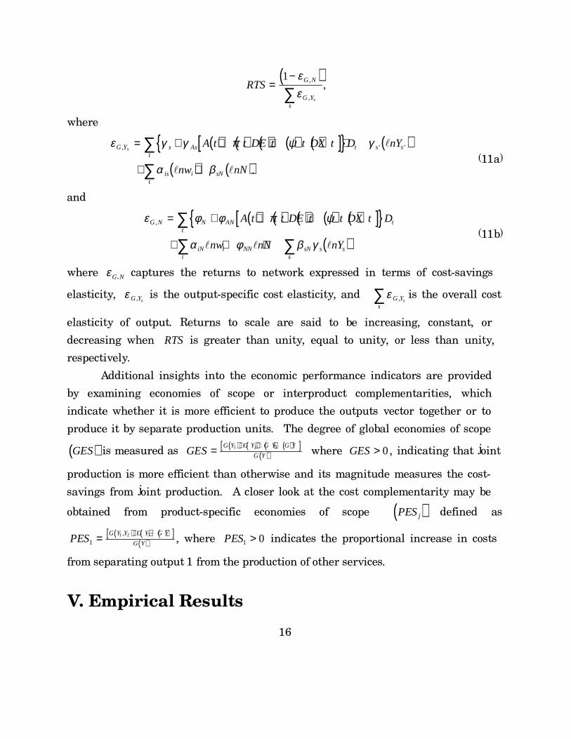
where εG N, captures the returns to network expressed in terms of cost-savings

elasticity, ε G Ys, is the output-specific cost elasticity, and ε G Ys

s,∑ is the overall cost

elasticity of output. Returns to scale are said to be increasing, constant, or

decreasing when RTS is greater than unity, equal to unity, or less than unity,

respectively.

Additional insights into the economic performance indicators are provided

by examining economies of scope or interproduct complementarities, which

indicate whether it is more efficient to produce the outputs vector together or to

produce it by separate production units. The degree of global economies of scope

( )GES is measured as ( ) ( ) ( ) ( )[ ]

( )GESG Y G Y G Y G Y

G Y= + + −1 2 3 where GES> 0 , indicating that joint

production is more efficient than otherwise and its magnitude measures the cost-

savings from joint production. A closer look at the cost complementarity may be

obtained from product-specific economies of scope ( )PESj defined as

( ) ( ) ( )[ ]( )PES

G Y Y G Y G Y

G Y11 2 3= + −,

, where PES1 0> indicates the proportional increase in costs

from separating output 1 from the production of other services.

V. Empirical Results

17

1. Parameter Estimates and Restrictions Tests

With a data set consisting of 710 observations on non-life insurance companies and

580 observations on life insurance companies for the period 1985-1995, an iterative

Zellner efficient estimation procedure was used on a system of a variable cost

function and two cost shares (labour and materials with the capital share

excluded). The parameter of both types of businesses were estimated separately for

the general model (equations (8) and (9)). The results are displayed in Tables II.

The standard tests for a well-behaved cost function were supportive. The results of

symmetry and concavity were not rejected. Homogeneity, however, was rejected for

P&C insurance only; nonetheless, it was imposed. As noted earlier, the exclusion

of multiproduct firms from the sample raises the issue of sample selection bias,

which occurs if the excluded firms differed systematically in their cost

characteristics from the included ones. Sample selection bias was therefore

investigated by testing that the inverse Mill�s ratio α h was significantly different

from zero. As shown by Tables II, the results suggest that the variable h captures

the otherwise missing information related to the excluded non-multiproduct firms.

[Insert Table II here]

The majority of the parameters in the estimated cost function are significant

at conventional levels and have the expected sign. The heterogeneity dummy

control variable λW is significant for both types of businesses and suggests that

mutual life insurance companies are more efficient than the reference case and

vice versa for non-life insurance companies. This represents a rejection in part of

the main prediction of prevailing economic theories of organizations, which argues

that because of impediments to monitoring managers� activities, mutual insurance

companies may be less efficient than stock insurance companies (see Fama and

Jensen 1985; Mayers and Smith 1988).

18

The results of the hypothesis tests using log-likelihood ratios are shown in

Table III. Sample selection bias related to the entry/exit of multiproduct firms was

investigated by testing the hypothesis ( ) ( )π ψt t= = 0 for t T= −2 3 1, ,..., . The results

indicate that this hypothesis is readily rejected at less than one percent, which

suggests that the selectivity bias that may result from entry / exist is an important

issue in my sample. The likelihood ratio tests suggest a decisive rejection of the

joint hypothesis that the coefficients related to the network are zero, suggesting

that this variable is meaningful in explaining the cost structure of insurance

companies. Also, the hypothesis that insurance companies have not experienced

technical progress of any kind was decisively rejected.

[Insert Table III here]

A further description of the production structure is provided by the Allen-

Uzawa partial elasticities of substitution and elasticities of demand. The entries in

Table IV indicate that for life and non-life insurance companies all own-price

elasticities are negative and statistically significant, a necessary condition for the

cost-minimizing factor-demand theory. The inputs can be ranked in the following

order of declining (in absolute value) price elasticity of demand: intermediate

inputs are by far more elastic than labour. With an elasticity of less than 0.05,

labour is the input whose own-price elasticity is the most inelastic. With regard to

the elasticities of substitution, the entries in Table IV indicate that labour and

intermediate inputs are substitutes and that both of them have a negative effect on

the shadow price of the network.

[Insert Table IV here]

2. Estimates of Economies of Scales and Scope

As previously discussed, in industries where firm size has two dimensions �that of

the service network and that of the magnitude of services �the interpretation of

19

scale economies is different from the conventional measure that uses the cost

elasticity of output. In fact, the inverse of the cost elasticity of output cannot be

interpreted as a measure of returns to scales (RTSs). Using the parameters

reported in Table II, RTSs were estimated. To provide insights into the groups� cost

characteristics over a reasonable range of the industry cost manifold, estimates of

RTSs were also derived for quartile sample output vectors. The quartile sample

mean output vectors were formed by ranking each output by type of business (life

and non-life insurance). These estimates were compared with those of returns to

scale where network effects are constrained to be zero (CRTS).

The results in Table V indicate that, for the overall sample mean output

vector, all types of businesses exhibit statistically significant CRTSs. The average

CRTSs for life insurance companies and P&C insurance companies are 1.08 and

1.02 respectively, which do not appear to be significantly different. This clearly

suggests that, in the absence of network effects, both life insurance and non-life

insurance businesses operate under constant RTSs. But the results show that the

CRTSs estimates vary substantially between the fourth output quartile and the

first quartile. For example, life and non-life insurance companies in the first

quartile exhibit relatively high and statistically significant CRTSs. By contrast,

the hypothesis of constant CRTSs cannot be rejected for these companies in the

fourth quartile. With regard to interbusiness comparisons, the results show that,

in general, life insurance companies display higher CRTSs than do their non-life

counterparts. This suggests that, unlike their life insurance counterparts, non-life

insurance companies incur higher incremental costs.

[Insert Table V here ]

By definition, the higher the cost-savings attributed to the availability of a

network ( ε G N, < 0), the higher the RTS. The results in Table V show that, for the

overall sample, mean output vectors of large firms exhibit statistically significant

RTS economies. The average of the RTSs for life insurance companies is 1.49, and

20

that of non-life insurance companies is 1.30. However, there are significant

differences in terms of RTSs between life and non-life insurance companies. Since

they are significant RTSs, this implies that a non-parametric estimate of TFP may

be a poor approximation of technical progress. Remarkably, although CRTSs

benefit mostly firms in the first and second quartiles, the cost-savings generated by

the presence of the network allows large life and non-life insurance companies

(those in the third and fourth quartiles) to display important economies of scales.

Analysis of economies of scope in the joint production of outputs provides

insight into the cost-savings from jointly producing insurance services relative to

producing each service individually. From the estimates in Table V, it appears

that, on average, there are global economies of scope for both life and non-life

insurance companies. Specifically, joint production is estimated to account for up

to 20 percent of cost-savings. Interestingly, for both types of businesses, these

savings become smaller as they move from the first to the last output quartile. In

the case of non-life insurance, however, the results indicate that product-specific

economies of scope exist for each type of service but do not exceed 9.6 percent on

average. Overall, the results suggest that, for non-life insurance companies,

greater savings can be achieved from the combination of all outputs as opposed to

the combination of one output with an existing output.

In summary, the empirical evidence suggests that, while CRTSs and cost-

savings complementarities are generally exhausted for the largest insurance firms,

the existence of substantial cost-savings generated by a network effect allows large

firms to display higher economies of scale. These results hold for both life and non-

life insurance companies. In addition, cost-savings from jointly producing

insurance services as opposed to individually producing each service are larger for

small and medium-sized firms, but they have the tendency to be exhausted in the

case of larger firms.

3. Estimates of Total Factor Productivity

21

Firms estimates of productivity growth were developed and then weighted as a

share of industry output to produce industry-level estimates of TFP and its

breakdown into technical change, scale economies, price-cost margin, and

temporary equilibrium effect. In Table VI, life insurance companies� TFP growth

was found to increase at an average annual rate of 2.6 percent for the period 1985-

1995. From 1985 to 1990, TFP grew at an average annual rate of roughly 3.4

percent. For the 1990-1993 period, a slight decline (only 2.1 percent) was detected

in the TFP growth, reflecting the effect of the business cycle. A slight recovery in

the TFP growth rate was noticeable during the subsequent recovery period (2.3

percent).

[Insert Table VI here]

It is of interest to see whether there are identifiable patterns of TFP between

life and non-life insurance companies. Inspection of entries in Table VI indicates

that, on average, life insurance companies enjoyed higher productivity growth than

their non-life counterparts. With an average annual growth of TFP as low as 0.8

percent, non-life insurance companies displayed an anemic productivity growth.

As for life insurance companies, most of the TFP growth took place during the

period of economic growth.4 During the period for which estimates of the

productivity of goods-producing industries and non-financial services industries

are comparable,5 that is 1985-1992, the TFP of life and non-life insurance business

grew, respectively, at an average annual rate of growth of 2.6% and .81%,

compared with a negative annual average rate of 0.39% for goods-producing

industries and 0.48% for non-financial services producing industries.

4 This result is in part due to the use of inappropriate deflators of non-life insurance output. Since

the value of insurance services considered in the non-life insurance component of the CPI are

constructed on the basis of the value of premiums (instead of premiums less claims plus investment

income), this has a tendency to overestimate the non-life insurance component of the CPI, which

results in an underestimation of my non-life insurance output.5 See Statistics Canada (1996).

22

As noted in (10), the estimated technical change index can in turn be broken

down into the effects caused by pure technical change, non-neutral technical

change, and scale-augmenting technical change. Table VI provides the results of

this breakdown for both life and non-life insurance companies for selected time

intervals. At 80 percent and 66 percent on average for life and non-life,

respectively, scale-augmenting technical change was the most important

component of technical change. It is followed well behind by non-neutral technical

change (18 percent and 34 percent, respectively, for life and non-life insurance).

The fact that life insurance companies� scale-augmenting technical change

contribution to technical change is higher than that of their non-life counterparts

may be related to government policy and the product innovations that have taken

place during the last two decades in the life insurance business. Government tax

policy has had a profound effect on life insurance companies� product mix. Apart

from a shift in product demand caused by tax changes (see Burbidge and Davies

1994), there has been a pronounced trend away from whole life policies and toward

term insurance. Policies that have encouraged savings through tax-sheltered

RRSPs have increased the demand for annuities. A large portion of each dollar of

whole life insurance premiums (compared with term insurance premiums for

example) is retained for the acquisition of assets because whole life insurance,

especially in a policy�s early years, contains a significant savings component.

Similarly, each dollar of deferred annuity premiums goes almost entirely to acquire

assets, which may be held for many years before liquidation. In this sense, the

change of life insurers� products influences the growth of this business.

The results displayed in Table VI show that scale economies have

contributed to more than 60 percent of insurance companies� TFP growth.

However, this contribution has been slightly declining for both life and non-life

insurance companies. The effect of market structures represents the third major

component of TFP growth after economies of scale and technical change. However,

the contribution of market structures to TFP growth is twice as high for non-life

23

insurance as it is for life insurance. There is evidence of imperfect competition in

the insurance business, particularly in the non-life insurance industry, as

suggested by a non-negligible contribution or price-cost margin to TFP growth.

Problems of information asymmetry in favour of the buyer may force firms to

charge higher prices to high-risk individuals.

Although the network size has experienced a positive, albeit small, year-

over-year growth rate, the effect of temporary equilibrium on TFP growth has

experienced three distinct trends during the 1985-1995 period. Although the effect

of temporary equilibrium was positive during the subperiod 1985-1990, it became

negative in the subsequent periods. The procyclical feature of the temporary

equilibrium effect mainly suggests that the long-run hypothesis underlying the

non-parametric TFP framework has been violated. A casual comparison of the

estimated value of the shadow price of network z with its market price r suggests

that, for the earlier years of the period 1985-1990, there was a strong incentive for

network investment, which ultimately led the industry to use the network to full

capacity.6 This trend was slightly reversed during the 1990-1993 subperiod as the

economy entered a recession, during which there was an apparent excess capacity

level of network. The incentive for additional network investment fell during this

period, however it increased slightly in the subsequent period as the economy

entered a period of recovey.

To provide insight on how company size may effect TFP, estimates of TFP

were also derived for the quartile sample output of life and non-life insurance

companies. Examination of the estimates of TFP growth for the quartile output

reveals a consistent pattern with other economic performance indicators such as

the constrained returns to scale and economies of scope. Chart 1, which plots TFP

for life and non-life insurance firms, shows a consistent pattern across quartiles.

6 During the period 1985-1991, the ratio q had an average annual growth rate of 18.3 percent for

life insurance and 12.1 percent for non-life insurance companies. Thereafter, it started to decrease to

7.4 percent and 11.2 percent, respectively.

24

Although TFP growth tends to decline as the size of the insurance firm,

productivity gains do not appear to be fully exhausted for large life insurance

firms.

[Insert Chart 1 here]

VI. Conclusion

With the proliferation of information technology over the past several decades,

networks have become increasingly important. Examples include banks�

automated teller machines, airlines� reservation systems, and the increased use of

the Internet. Although networks have been shown to have important implications

on firms� strategies for product announcement, technology adoption, and pricing

(see Katz and Shapiro 1985), there has been no attempt to measure the effects of

networks on firms� cost structures.

In this paper, a short-run cost function defined over a vector of output and

the size of insurance companies� network was specified and estimated for an

incomplete panel data set of Canadian life and non-life insurance companies. RTSs

were found to be large and statistically significant, particularly for large insurance

companies, as cost-savings associated with the existence of a network of agents and

brokers allows large firms to exhibit increasing returns to scale in the short run.

Failure to account for network effects has led many previous studies using

different national data to conclude that large firms operate under constant RTSs.

Changes in TFP through time are hypothesized to be the result of scale

economies, technical change, market structures, and the temporary equilibrium

associated with the existence of a network with a given size in the short run. The

findings indicate that although life insurance companies out perform their non-life

counterparts in terms of TFP growth, the bulk of this growth for both types of firms

is a result of scale economies and technical change. There is evidence of imperfect

25

competition in the insurance business, particularly in the non-life insurance

industry, as suggested by a non-negligible contribution or price-cost margin to TFP

growth. Problems of information asymmetry in favour of the buyer may force firms

to charge higher prices to high-risk individuals.

There is strong evidence that the long-run hypothesis underlying the non-

parametric TFP framework has been violated. The results suggest that, in general,

the level of various economic performance indicators declines with the firm size.

This indicates that, unlike medium-sized firms, large ones have exhausted their

potential for economic performance. Although there are variants across

businesses, this result holds for both life and non-life insurance companies.

26

References

Baltagi B.H. and J. M. Griffin (1988); �A General Index of Technical Change,�

Journal of Political Economy 96: 20-41.

Berndt, E.R. and M.A. Fuss (1986); �Productivity Measurement with Adjustments

for Variations in Capacity Utilization and Other Forms of Temporary Equilibrium,�

Journal of Econometrics .

Bernstein, J.I. (1992); �Information Spillovers, Margins, Scale and Scope: With an

Application to Canadian Life Insurance,� Scandinavian Journal of Economics 94

(Supplement): 95-105.

Braeutigam, R.R. and M.V. Pauly (1986); �Cost-Function Estimation and Quality

Bias: The Regulated Automobile Insurance Industry,� Rand Journal of Economics

17: 606-617.

Burbidge, J.B. and Davies, J.B. (1994); �Government Incentives and Household

Saving in Canada,� in Poterba J. (Ed.): Public Policies and Household Saving,

pp. 19-56, Chicago University Press for the NBER, Chicago.

Caves, D.W., L.T. Christensen and J.A. Swanson (1981); �Productivity Growth,

Scale Economies, and Capacity Utilization in U.S. Railroads, 1955-74,� American

Economic Review 71: 994-1002.

Dagenais M.G. and J.-M. Dufour (1992); �Invariance, Nonlinear Models, and

Asymptotic Tests,� Econometrica 89: 1601-15.

Daly, M.J., P.S. Rao and R.R. Geehan (1985); �Productivity, Scale Economies and

Technical Progress in the Canadian Life Insurance Industry,� International

Journal of International Organizations 3: 345-61.

Denny, M., M. Fuss, and L. Waverman (1981); �The Measurement and

Interpretation of Total Factor Productivity in Regulated Industries, with an

Application to Canadian Telecommunications in Cowing T.G. and R.E. Stevenson

(eds.): Productivity Measurement in Regulated Industries, Academic Press.

Diewert, E.W. (1982); Duality Approaches to Microeconomic Theory, in Arrow, K.

and M. Intriligator (eds.): Handbook of Mathematical Economics, Vol. II,

Elsevier Science Publishers, The Netherlands.

27

Dionne, G. and R. Gagné (1992); �Measuring Technical Change and Productivity

Growth with Varying Output Qualities and Incomplete Panel Data,� Université de

Montréal, Département de sciences économiques, cahier 9201.

Fama, E.F. and M. Jensen (1985); �Organizational Forms and Investment

Decisions,� Journal of Financial Economics , 14: 101-19.

Globerman, S. (1984); The Adoption of Computer Technology by Insurance

Companies, Ottawa, Supply and Services Canada.

Grace M.F. and S.G. Timme (1993); �An Examination of Cost Economies in the

United States Life Insurance Industry,� Journal of Risks and Insurance 93: 72-103.

Heckman (1979), J. �Sample Selection Bias as a Specification Error,� Econometrica

47: 153-161.

Hunter, W.C. and S.G. Timme (1993); �Core Deposits and Physical Capital: A Re-

examination of Bank Scale Economies and Efficiency with Quasi-Fixed Inputs,�

Federal Reserve Bank of Atlanta Working Paper 93-3.

Mayers, D. and C. Smith (1988); �Ownership Structure Across Lines of Property

and Casualty Insurance,� Journal of Law Economics 31: 351-78.

Olley, S. and A. Pakes (1991); �The Dynamics of Productivity in the

Telecommunications Equipment Industry, Department of Economics, Yale

University, New Haven, CT.

Saloner G. and A. Shephard (1995); �Adoption of Technologies with Network Effect:

An Emprical Examination of the Adoption of Automated Teller Machines,� Rand

Journal of Economics 26: 479-501.

Statistics Canada (1996); Aggregates Productivity Measures (Annual),

Catalogue 15-204-XPE, Ottawa.

Suret, J.-M. �Scale and Scope Economies in the Canadian Property and Casualty

Insurance Industry,� Geneva Papers of Risk and Insurance 89: 236-56.

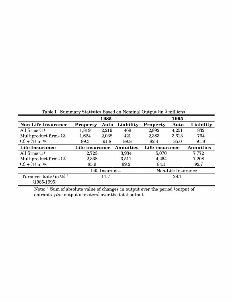
Table I. Summary Statistics Based on Nominal Output (in $ millions)

1985 1995

Non-Life Insurance Property Auto Liability Property Auto Liability

All firms (1) 1,819 2,219 469 2,892 4,251 832Multiproduct firms (2) 1,624 2,038 421 2,383 3,613 764(2) ÷ (1) in % 89.3 91.8 89.8 82.4 85.0 91.8

Life Insurance Life insurance Annuities Life insurance Annuities

All firms (1) 2,723 3,934 5,070 7,772Multiproduct firms (2) 2,338 3,511 4,264 7,208(2) ÷ (1) in % 85.9 89.2 84.1 92.7

Life Insurance Non-Life InsuranceTurnover Rate (in %)

a

(1985-1995)11.7 28.1

Note: a Sum of absolute value of changes in output over the period (output of

entrants plus output of exiters) over the total output.

Table IIa. Parameter Estimates of Life Insurance Companies�Short-Run Cost Function with a General Index of Technical Change

Variable Estimate t − statistic Variable Estimate t − statisticα o 3.0512 2.113 ( )π 86 0.0912 1.611

α L 0.2214 3.710 ( )π 87 0.0312 1.809

α M 0.1296 2.811 ( )π 88 0.0102 1.611

γ YL0.1081 3.126 ( )π 89 0.0512 1.987

γ YA0.2342 5.234 ( )π 90 0.1012 2.876

φ N 0.2813 2.313 ( )π 91 0.0399 2.011

α LL 0.1511 2.411 ( )π 92 0.0093 1.311

α MM 0.0512 1.934 ( )π 93 0.0023 1.098

α LM -0.0113 2.915 ( )π 94 0.0102 1.134

α LYL0.0912 2.981 ( )ψ 86 -0.0198 1.013

α LYA0.1123 2.673 ( )ψ 87 -0.0145 1.997

α MYL-0.0221 1.875 ( )ψ 88 -0.0449 2.018

α MYA-0.0102 1.773 ( )ψ 89 -0.0711 2.012

α LA 0.0051 2.121 ( )ψ 90 -0.1298 1.978

α MA -0.0155 2.127 ( )ψ 91 -0.0823 3.129

α LN 0.0114 2.174 ( )ψ 92 -0.4412 3.129

α MN 0.0128 2.861 ( )ψ 93 -0.4012 2.455

γ Y YL L0.2312 3.481 ( )ψ 94 -0.3866 2.523

γ Y YA A0.3581 4.534 ( )A 86 -0.1011 2.011

γ Y YL A0.0871 2.012 ( )A 87 -0.0978 2.801

φ NN -0.2253 2.413 ( )A 88 -0.0489 3.912

γ AYL0.0124 3.167 ( )A 89 -0.0712 2.012

γ AYA0.1131 5.234 ( )A 90 -0.1123 3.123

φ AN 0.0923 2.451 ( )A 90 -0.1123 3.123

βY NL0.2192 5.221 ( )A 91 -0.1245 3.891

βY NA0.3381 3.819 ( )A 92 -0.0778 5.897

λ W -0.0812 2.871 ( )A 93 -0.0983 3.089

α h 1.310 4.023 ( )A 94 -0.1377 4.912

( )A 95 -0.1012 3.091

Equation Std. Error R2

Cost 0.06156 0.94Labour Share 0.02267 0.87

Intermediate Input Share 0.01912 0.84Log of Likelihood 2,723

Table IIb. Parameter Estimates of Non-Life Insurance Companies�Short-Run Cost Function with a General Index of Technical Change

Variable Estimate t − statistic Variable Estimate t − statisticα o 0.0102 3.467 βY NA

0.0123 1.667

α L 0.1169 1.982 βY NL0.1711 3.123

α M 0.0914 1.758 λ W 0.1226 4.121γ YP

0.0774 4.125 α h 2.017 3.148γ YA

0.1281 3.339 ( )π 86 0.0107 1.981

γ YL0.2341 4.181 ( )π 87 0.0212 2.016

φ N 0.3112 4.167 ( )π 88 0.0314 3.117

α LL 0.0912 1.912 ( )π 89 0.0174 3.339

α MM 0.0417 2.012 ( )π 90 0.0471 4.125

α LM -0.0221 1.698 ( )π 91 0.0701 1.974

α LYP0.0152 1.711 ( )π 92 0.0093 2.447

α LYA0.0781 1.991 ( )π 93 0.0023 0.557

α LYL0.1023 3.012 ( )π 94 0.0097 2.007

α MYP-0.0981 1.814 ( )ψ 86 -0.0077 1.147

α MYA-0.0114 2.115 ( )ψ 87 -0.0142 2.227

α MYL-0.1098 3.119 ( )ψ 88 -0.0314 1.781

α LA 0.0088 3.874 ( )ψ 89 -0.0591 3.227

α MA -0.0978 1.689 ( )ψ 90 -0.0798 4.126

α LN 0.0447 1.978 ( )ψ 91 -0.0516 2.474

α MN 0.0011 1.551 ( )ψ 92 -0.1293 2.987

γ Y YP P0.1102 1.997 ( )ψ 93 -0.1147 3.074

γ Y YA A0.1477 2.411 ( )ψ 94 -0.0071 2.851

γ Y YL L0.1827 2.866 ( )A 86 -0.0367 3.157

γ Y YP A0.0275 1.886 ( )A 87 -0.0407 1.889

γ Y YP L0.0981 2.113 ( )A 88 -0.0566 2.471

γ Y YA L0.1366 4.129 ( )A 89 -0.0889 9.771

φ NN -0.1652 4.336 ( )A 90 -0.1202 2.971

γ AYP0.0234 2.110 ( )A 90 -0.1011 2.339

γ AYA0.0761 1.997 ( )A 91 -0.0833 4.117

γ AYL0.1183 4.125 ( )A 92 -0.0519 2.997

φ AN 0.07112 3.667 ( )A 93 -0.0711 2.339

βY NP0.0543 1.714 ( )A 94 -0.1209 5.971

( )A 95 -0.1488 2.789

Equation Std. Error R2

Cost 0.09367 0.89Labour Share 0.05147 0.84

Intermediate Input Share 0.02204 0.81Log of Likelihood 2,507

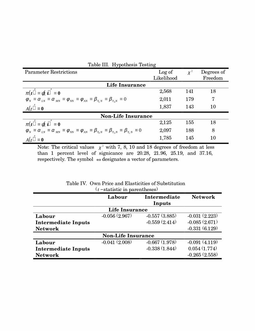
Table III. Hypothesis Testing

Parameter Restrictions Log ofLikelihood

χ 2 Degrees ofFreedom

Life Insurance

( ) ( )π ψt t′ = ′ = 0 2,568 141 18

φ α α φ φ β βN LN MN NN AN Y N Y NL A= = = = = = = 0 2,011 179 7

( )A t′ = 0 1,837 143 10

Non-Life Insurance

( ) ( )π ψt t′ = ′ = 0 2,125 155 18

φ α α φ φ β β βN LN MN NN AN Y N Y N Y NP A L= = = = = = = = 0 2,097 188 8

( )A t′ = 0 1,785 145 10

Note: The critical values χ 2 with 7, 8, 10 and 18 degrees of freedom at lessthan 1 percent level of signicance are 20.28, 21.96, 25.19, and 37.16,respectively. The symbol ©�ª designates a vector of parameters.

Table IV. Own Price and Elasticities of Substitution(t −statistic in parentheses)

Labour Intermediate

Inputs

Network

Life Insurance

Labour -0.056 (2.967) -0.557 (3.885) -0.031 (2.223)

Intermediate Inputs -0.559 (2.414) -0.085 (2.671)

Network -0.331 (6.129)

Non-Life Insurance

Labour -0.041 (2.008) -0.667 (1.978) -0.091 (4.119)

Intermediate Inputs -0.338 (1.844) 0.054 (1.774)

Network -0.265 (2.558)

Table V. Estimates of Returns to Scale and Returns to Scopeby Quartile and by Type of Business

(Asymptotic standard errors in parenthesis)

Type of Businessand Ownership

Overall 1stQuartile

2ndQuartile

3rdQuartile

4thQuartile

Constrained Returns to Scalea

Life insurance 1.08 1.18 1.21 1.05 1.02Non-life insurance 1.02 1.12 1.16 1.03 1.01

Returns to Scale

Life insurance 1.49 1.39 1.38 1.45 1.54Non-life insurance 1.30 1.24 1.24 1.36 1.48

Economies of Scope

Life Insurance

GES .271 .345 .272 .163 .087

Non-Life Insurance

GES .219 .236 .221 .114 .111PES (Property) .061 .094 .081 .063 .055PES (Auto) .096 .124 .103 .082 .063PES (Liability) .074 .131 .084 .065 .044

Note: a It is a measure of returns to scale where the effect of network is

constrained to be zero; all estimates are significant at least at the 5 percentlevel of significance; GES = global economies of scope, PES = product-specific economies of scope.

Table VI. Total Factor Productivity Growth and Its Sources

Percentage Contribution to TFP of

TimePeriod

TFPin %

Non-ConstantReturnsto Scale

Technical Progress TemporaryEquilibrium

Price-Cost

Margin

�T Pure Scaleaugmentation

Non-neutral

Life Insurance

1985-1990 3.4 74.5 18.4 3.5 83.8 12.7 0.5 6.61990-1993 2.1 71.2 24.7 3.4 78.1 18.5 -3.1 7.21993-1995 2.3 69.5 28.5 1.4 76.5 22.1 -2.9 4.9Average 2.6 71.7 23.8 2.8 79.5 17.8 -1.8 6.2

Non-Life Insurance

1985-1990 .91 70.1 14.1 .5 70.4 29.1 4.1 11.71990-1993 .73 62.0 25.2 1.9 63.9 34.2 -1.4 14.21993-1995 .79 56.9 28.5 .5 61.2 38.3 -1.1 15.7

Average .81 63.0 22.6 .97 65.2 33.9 .53 13.9

7)3�$YHUDJH�$QQXDO�*URZWK�5DWH�

%\�)LUP�6L]H�����������

�

���

�

���

�

���

�

�VW

4XDUWLOH

�QG

4XDUWLOH

�UG

4XDUWLOH

�WK

4XDUWLOH

/LIH�,QVXUDQFH 1RQ�/LIH�,QVXUDQFH