the economic effects of constitutions, what do the data say?

THE ECONOMIC EFFECTS OF CONSTITUTIONS

What do the data say?*

Torsten Persson and Guido Tabellini

October 6, 2002

*To be published by MIT Press, August 2003

To Our Mothers

1

Preface

This book is intended for the scholar or graduate student who wants to learnabout a new topic of research: the effects of constitutional rules on economicpolicymaking and performance. We draw on existing knowledge in several fields:economics, political science, and statistics. In particular, the book builds ontheoretical work from the last few years, and it forms a natural sequel to ourprevious book, Political Economics: Explaining Economic Policy, published byMIT Press in the year 2000. While the previous volume focused mainly ontheory, the purpose of this new book is uncompromisingly empirical. Takingthe existing theoretical work in comparative politics and political economicsas a point of departure, we ask which theoretical results are supported andcontradicted by the data, and try to identify new empirical patterns for a nextround of theory.The empirical results we present in the book go beyond those in our recent

articles and working papers on the same general topic. But there are other rea-sons why the entire thing is greater than the sum of its parts. We take advantageof the book format to present a more thorough discussion of measurement andmethodology than is possible in a single paper. In the end, the empirical picturestands out quite clearly and convincingly, when considering a number of relatedissues with a similar methodology.Our decision to embark on the empirical research program resulting in the

book was taken when one of us (Tabellini) gave the Munich Lectures, hostedby CES, in November 1999. At that point, we had produced several theoreticalstudies of constitutional rules and economic policy, but we had only started tolook at the data and our empirical results were still preliminary. The commentsreceived from the Munich audience, and in particular from Hans-Werner Sinnand Vito Tanzi, were an essential input and inspiration for the research thatfollowed. The warm hospitality and the outstanding atmosphere of excitementand enthusiasm at CES made those lectures a particularly memorable event.Another event that helped focus our minds, when this project was further

under way, was the Walras-Bowley Lecture, given by one of us (Persson) at theEconometric Society World Congress in Seattle, August 2000. On this occasion,as well, we obtained important feedback that led to major improvements in ourresearch.After having completed a first full draft, in May 2002, we had the opportu-

nity to present overviews of the manuscript to different audiences in Uppsala,Princeton, Harvard, the European Science Days in Steyr, Austria, and the YrjöJahnsson Foundation, in Helsinki.At these presentations, and at numerous seminars on the underlying research

papers, many colleagues made insightful comments that improved the qualityof our research. Here, we particularly want to thank our colleagues who gen-erously gave up their time for reading and commenting on the first draft: JimAlt, Tim Besley, Robin Burgess, Jon Faust, Jeff Frieden, Emanuel Kohlscheen,Per Molander, Olof Petersson, Per Pettersson-Lidbom, Gérard Roland, LudgerSchuknecht, Rolf Strauch, David Strömberg, Jakob Svensson, and three anony-

1

mous MIT Press readers. We also owe special gratitude to Andrea Ichino, aswell as Richard Blundell, Hide Ichimura, and Costas Meghir, whose commentson our empirical papers were instrumental in directing us towards some of theeconometric methodology that figures so prominently in the book.Putting together the two data sets used in this book involved a great deal of

work on data collection, data-base management, and estimation. We were luckyenough to benefit from expert help with these tasks by a number of researchassistants from different cohorts of graduate students: Gani Aldashev, AlessiaAmighini, Alessandra Bonfiglioli, Agostino Consolo, Thomas Eisensee, GiovanniFavara, Jose Mauricio Prado Jr., Andrea Mascotto, Alessandro Riboni, DavideSala and Francesco Trebbi (also a co-author of one of our articles). We benefitedgreatly from their efforts, as will other researchers with free access to the datasets used in the book.The last stretch of work on a book manuscript can be an open-ended period

of frustration, when every chapter, table, figure, and footnote seems to be inconstant flux imposed by authors’ desperate last-minute changes, as well as thepublisher’s rigorous style requirements. Luckily, in this case, as in our previousbook project, we could rely on the outstanding assistance of Christina Lönnblad.We are deeply grateful to her for helping us out with editing and style, and forcheerfully putting in some long hours, also on free days and weekends. We arealso very grateful to Lorenza Negri for her efficient and professional editorialassistance in various stages of the project.While the initial agreement with MIT Press was made with Terry Vaughn,

he left for greener pastures before the book was seriously on its way. We aregrateful to our editor, John Covell, for taking over and for being patient withour changing schedule, as we were gradually upgrading our ambitions for thefinal product.Finally, we gratefully acknowledge financial support for the research program

underlying this book from a number of sources: Bocconi University, LondonSchool of Economics, MURST, and the Italian and Swedish Research Councils.

Stockholm and Milan, October 2002

2

Contents

1 Introduction and overview 7

1.1 Constitutions and policy: a missing link . . . . . . . . . . . . 81.2 Which constitutional rules and policies? . . . . . . . . . . . . 111.3 Overview of the book . . . . . . . . . . . . . . . . . . . . . . . 13

2 What does theory say? 172.1 Introduction . . . . . . . . . . . . . . . . . . . . . . . . . . . . 172.2 A common approach . . . . . . . . . . . . . . . . . . . . . . . 192.3 Electoral rules . . . . . . . . . . . . . . . . . . . . . . . . . . . 21

2.3.1 District magnitude . . . . . . . . . . . . . . . . . . . . 222.3.2 Electoral formula . . . . . . . . . . . . . . . . . . . . . 252.3.3 Ballot structure . . . . . . . . . . . . . . . . . . . . . . 262.3.4 Empirical predictions . . . . . . . . . . . . . . . . . . . 26

2.4 Forms of government . . . . . . . . . . . . . . . . . . . . . . . 272.4.1 Separation of powers . . . . . . . . . . . . . . . . . . . 282.4.2 Confidence requirement . . . . . . . . . . . . . . . . . . 282.4.3 Empirical predictions . . . . . . . . . . . . . . . . . . . 30

2.5 Related ideas . . . . . . . . . . . . . . . . . . . . . . . . . . . 302.6 What questions do we pose to the data? . . . . . . . . . . . . 342.7 The empirical agenda . . . . . . . . . . . . . . . . . . . . . . . 36

3 Policy measures and their determinants 393.1 Introduction . . . . . . . . . . . . . . . . . . . . . . . . . . . . 393.2 Fiscal policy . . . . . . . . . . . . . . . . . . . . . . . . . . . . 41

3.2.1 Size of government . . . . . . . . . . . . . . . . . . . . 413.2.2 Composition of government . . . . . . . . . . . . . . . 503.2.3 Budget surplus . . . . . . . . . . . . . . . . . . . . . . 52

3

4 CONTENTS

3.3 Rent extraction . . . . . . . . . . . . . . . . . . . . . . . . . . 543.3.1 Measuring corruption . . . . . . . . . . . . . . . . . . . 543.3.2 Determinants of corruption . . . . . . . . . . . . . . . 56

3.4 Productivity and policy . . . . . . . . . . . . . . . . . . . . . 593.4.1 Measuring productivity and growth promoting policies 603.4.2 Determinants of productivity and growth promoting

policies . . . . . . . . . . . . . . . . . . . . . . . . . . . 62

4 Electoral rules and forms of government 694.1 Introduction . . . . . . . . . . . . . . . . . . . . . . . . . . . . 694.2 Which countries and years? . . . . . . . . . . . . . . . . . . . 70

4.2.1 Defining democracies . . . . . . . . . . . . . . . . . . . 714.2.2 Dating democracies . . . . . . . . . . . . . . . . . . . . 73

4.3 Electoral rules . . . . . . . . . . . . . . . . . . . . . . . . . . . 754.3.1 Basic measures of electoral rules . . . . . . . . . . . . . 764.3.2 Dating of electoral rules . . . . . . . . . . . . . . . . . 784.3.3 Continuous measures of electoral rules . . . . . . . . . 80

4.4 Forms of government . . . . . . . . . . . . . . . . . . . . . . . 834.4.1 A basic measure of forms of government . . . . . . . . 844.4.2 Dating of forms of government . . . . . . . . . . . . . . 86

4.5 Our political atlas . . . . . . . . . . . . . . . . . . . . . . . . . 884.6 Constitutions, performance and co-variates: a first look . . . . 90

4.6.1 Constitutions and outcomes . . . . . . . . . . . . . . . 904.6.2 Constitutions and other co-variates . . . . . . . . . . . 93

5 Cross-sectional inference: Pitfalls and methods 955.1 Introduction . . . . . . . . . . . . . . . . . . . . . . . . . . . . 955.2 The question . . . . . . . . . . . . . . . . . . . . . . . . . . . 98

5.2.1 Primitives . . . . . . . . . . . . . . . . . . . . . . . . . 985.2.2 The parameter of interest . . . . . . . . . . . . . . . . 1005.2.3 Estimation . . . . . . . . . . . . . . . . . . . . . . . . . 101

5.3 Simple linear regressions . . . . . . . . . . . . . . . . . . . . . 1035.3.1 Conditional independence . . . . . . . . . . . . . . . . 1035.3.2 Linearity . . . . . . . . . . . . . . . . . . . . . . . . . . 1045.3.3 Ordinary Least Squares . . . . . . . . . . . . . . . . . 105

5.4 Relaxing conditional independence . . . . . . . . . . . . . . . 1085.4.1 Instrumental variables . . . . . . . . . . . . . . . . . . 1085.4.2 Adjusting for selection . . . . . . . . . . . . . . . . . . 113

CONTENTS 5

5.5 Relaxing linearity . . . . . . . . . . . . . . . . . . . . . . . . . 1175.5.1 Matching estimators . . . . . . . . . . . . . . . . . . . 1185.5.2 Propensity scores . . . . . . . . . . . . . . . . . . . . . 1195.5.3 Implementation . . . . . . . . . . . . . . . . . . . . . . 122

5.6 Multiple constitutional states . . . . . . . . . . . . . . . . . . 127

6 Fiscal Policy: Variation across countries 1296.1 Introduction . . . . . . . . . . . . . . . . . . . . . . . . . . . . 1296.2 Size of government . . . . . . . . . . . . . . . . . . . . . . . . 132

6.2.1 OLS estimates . . . . . . . . . . . . . . . . . . . . . . . 1326.2.2 IV and Heckman estimates . . . . . . . . . . . . . . . . 1356.2.3 Matching estimates . . . . . . . . . . . . . . . . . . . . 1376.2.4 Summary . . . . . . . . . . . . . . . . . . . . . . . . . 139

6.3 Composition of government . . . . . . . . . . . . . . . . . . . 1406.3.1 OLS estimates . . . . . . . . . . . . . . . . . . . . . . . 1406.3.2 IV and Heckman estimates . . . . . . . . . . . . . . . . 1446.3.3 Matching estimates . . . . . . . . . . . . . . . . . . . . 1456.3.4 Summary . . . . . . . . . . . . . . . . . . . . . . . . . 146

6.4 Budget surplus . . . . . . . . . . . . . . . . . . . . . . . . . . 1466.4.1 OLS estimates . . . . . . . . . . . . . . . . . . . . . . . 1476.4.2 Heckman estimates . . . . . . . . . . . . . . . . . . . . 1486.4.3 Matching estimates . . . . . . . . . . . . . . . . . . . . 1496.4.4 Summary . . . . . . . . . . . . . . . . . . . . . . . . . 149

6.5 Concluding remarks . . . . . . . . . . . . . . . . . . . . . . . . 150

7 Political rents and productivity: Variation across countries 1537.1 Introduction . . . . . . . . . . . . . . . . . . . . . . . . . . . . 1537.2 Political rents . . . . . . . . . . . . . . . . . . . . . . . . . . . 156

7.2.1 OLS estimates . . . . . . . . . . . . . . . . . . . . . . . 1577.2.2 IV and Heckman estimates . . . . . . . . . . . . . . . 1607.2.3 Matching estimates . . . . . . . . . . . . . . . . . . . . 1627.2.4 Summary . . . . . . . . . . . . . . . . . . . . . . . . . 163

7.3 Productivity . . . . . . . . . . . . . . . . . . . . . . . . . . . . 1637.3.1 Reduced-form estimates . . . . . . . . . . . . . . . . . 1647.3.2 Structural-form estimates . . . . . . . . . . . . . . . . 1667.3.3 Endogenous selection . . . . . . . . . . . . . . . . . . . 1697.3.4 Matching estimates . . . . . . . . . . . . . . . . . . . . 1717.3.5 Summary . . . . . . . . . . . . . . . . . . . . . . . . . 172

6 CONTENTS


8 Fiscal policy: Variation across time 1758.1 Introduction . . . . . . . . . . . . . . . . . . . . . . . . . . . . 1758.2 Methodology . . . . . . . . . . . . . . . . . . . . . . . . . . . 177

8.2.1 The question . . . . . . . . . . . . . . . . . . . . . . . 1778.2.2 Estimation . . . . . . . . . . . . . . . . . . . . . . . . . 179

8.3 Unobserved common events . . . . . . . . . . . . . . . . . . . 1818.3.1 Size of government . . . . . . . . . . . . . . . . . . . . 1838.3.2 Welfare spending . . . . . . . . . . . . . . . . . . . . . 1868.3.3 Budget surplus . . . . . . . . . . . . . . . . . . . . . . 1888.3.4 Summary . . . . . . . . . . . . . . . . . . . . . . . . . 189

8.4 Output gaps . . . . . . . . . . . . . . . . . . . . . . . . . . . . 1908.4.1 Size of government . . . . . . . . . . . . . . . . . . . . 1918.4.2 Welfare spending . . . . . . . . . . . . . . . . . . . . . 1948.4.3 Budget surplus and government revenue . . . . . . . . 1968.4.4 Summary . . . . . . . . . . . . . . . . . . . . . . . . . 197

8.5 Elections . . . . . . . . . . . . . . . . . . . . . . . . . . . . . . 1988.5.1 Unconditional electoral cycles . . . . . . . . . . . . . . 2018.5.2 Proportional vs. majoritarian democracies . . . . . . . 2038.5.3 Parliamentary vs. presidential democracies . . . . . . . 2058.5.4 A four-way constitutional split . . . . . . . . . . . . . . 2078.5.5 Summary . . . . . . . . . . . . . . . . . . . . . . . . . 208


9 What have we learned? 2119.1 Theoretical priors and empirical results . . . . . . . . . . . . . 211

9.1.1 Electoral rules . . . . . . . . . . . . . . . . . . . . . . . 2129.1.2 Forms of government . . . . . . . . . . . . . . . . . . . 215

9.2 What next? . . . . . . . . . . . . . . . . . . . . . . . . . . . . 217

Chapter 1

Introduction and overview

Since the 1990s, constitutional reforms are the subject of heated debate inmany democracies. Debate has already led to a number of important reforms.Among the industrial countries, Italy left its former reliance on full propor-tional representation (PR), introducing a first-past-the-post system for 75%of the seats in the National Assembly. Similarly, New Zealand introduced amixed PR-plurality system, but from the opposite point of departure — thetraditional British system of appointing all lawmakers by plurality rule inone-member constituencies. Japan also renounced its special form of plural-ity voting in favor of a mixed system. In Latin America, Bolivia, Ecuadorand Venezuela undertook large-scale electoral reform in the 1990s, as did Fijiand the Philippines.Other reforms are still under debate. In the UK, discussions about switch-

ing to a mixed or proportional electoral system have resurfaced. In Italy, keypolitical leaders consider proposals of injecting elements of presidentialism orsemi-presidentialism into the current parliamentary regime, while in Francesome commentators would like to go the other way, towards more parlia-mentarism. Alternative ideas of how to address inefficient decision-makingand the “democratic deficit” in the European Union, involve constitutionalreforms introducing clearer principles of either parliamentary or presidentialdemocracy at the European level.These constitutional discussions often concern the alleged effects of con-

stitutional reforms on economic policy and economic performance.1 Is it

1The contributions in Shugart and Wattenberg (2001) discuss the motives behind, andthe political consequences of, reform in these and other countries adopting mixed electoral

7

8 CHAPTER 1. INTRODUCTION AND OVERVIEW

true that a move towards more majoritarian elections would stifle corruptionamong politicians, as presumed by the vast majority of Italians who approvedthe electoral reform? Would it also reduce the propensity of Italian govern-ments to run budget deficits? If the UK were to abandon its current first-past-the-post system in favor of proportional elections, would this change the sizeof overall government spending or the welfare state? Can we really blame thepoor and volatile economic performance of many countries in Latin Americaon their presidential form of government? More generally, what are the eco-nomic effects of constitutional reforms? Knowing the answers to these typesof questions is important not only for established democracies contemplatingreform, but also for new democracies designing their constitutions more fromscratch.The goal of this book is to contribute to the body of empirical knowledge

about these very difficult, yet fundamental, issues.

1.1 Constitutions and policy: a missing linkSurprising as it may seem, social scientists have not really addressed thequestion of constitutional effects on economic policy and economic perfor-mance, until very recently. In fact, some observers have even gone as far asdeeming it impossible to predict the consequences of constitutional reforms(Elster and Slagstad, 1988). But this is clearly an extreme position. Analyz-ing the effects of alternative constitutions is a main research topic in politicalscience, as exemplified by the contributions of Sartori (1994), Bingham Pow-ell (1982), Lijphart (1984), to name just a few. Yet, despite this long andhonored tradition, little is known empirically about the economic effects ofalternative constitutions.To see why, consider the stylized view of the democratic policymaking

process in Figure 1.1. Citizens and groups in society have conflicting prefer-ences over economic policy. Political institutions aggregate these preferencesinto specific political outcomes and these in turn induce public-policy deci-sions in the economic domain (the arrows on the right in the figure). Publicpolicies interact with markets and influence the prices of different goods, em-ployment and remunerations in different sectors of the economy, and thesemarket outcomes feed back into policy preferences (the arrows on the left).In this view of the interaction between politics and economics, the formal

systems in the 1990s.

1.1. CONSTITUTIONS AND POLICY: A MISSING LINK 9

rules of the constitution influence political decisions over economic policy,given some distribution of (primitive) preferences over economic outcomes inthe population. Our goal is to learn more about the effects of these formalconstitutional rules on specific economic policies.

Figure 1.1 about here

The box on the right-hand side of Figure 1.1 is the domain of traditionalcomparative politics. Political scientists in this field of research have spentdecades working on the fundamental features of constitutions and their po-litical effects. Apart from a few recent exceptions mentioned below and inChapter 2, however, this research does not reach beyond political phenomena:how different electoral systems affect the number of parties or the incidenceof coalition governments, how the form of government affects the frequencyof government crises and political instability, and so on. In terms of Figure1.1, the political-science research on constitutions has remained within theconfines of the box to the right, dealing with the link between constitutionalrules and political outcomes. Yet, the conclusions often point squarely in thecontinuation of this arrow, i.e., towards an investigation of systematic pol-icy consequences. For example, the comparative politics literature portraysthe choice between majoritarian and proportional elections, as a trade-offbetween accountability and representation.2 It is plausible that this choicewill be reflected in observable economic-policy consequences: better account-ability might show up in less corruption, and broader representation in morecomprehensive social-insurance programs. A few political scientists have re-cently asked the empirical “so-what” question of how constitutional rulesinfluence economic policy. Largely based on simple correlations in relativelysmall data sets of developed democracies, these studies have not come upwith clear-cut evidence of a mapping from electoral rules, or forms of gov-ernment, to policy outcomes.3

2The recent book by Bingham Powell (2000), for example, makes this point very clearlyand thoroughly.

3Lijphart (1999) asks a so-what question about some macroeconomic outcomes, in-cluding budget deficits, in different democracies classified largely by their electoral rules.Using mainly bivariate correlations in a sample of 36 countries, he finds few systematiceffects. Castles (1998) studies possible determinants of economic policy, including thesize of government and the welfare state in 21 developed OECD democracies. One of thedeterminants is an institutional indicator, mixing five different constitutional provisions,


It is not fair to say that all research in political science has remained insidethe box on the right hand side of the figure. Another substantial political-science literature relates economic policy to political outcomes, such as partystructure or political instability. But these political outcomes are typicallytaken as the starting point of the analysis and they are not explicitly linkedto specific constitutional features. This can be illustrated as a study of thearrow from “Political outcomes” to “Policy decisions” in Figure 1.1. Sincethe political outcomes are indeed systematically related to the constitutionalrules we study in this book (electoral rules, e.g., help shape the party struc-ture), this research is also relevant for our main question and we discuss itfurther in Chapter 2.The box on the left-hand side of Figure 1.1 is the domain of traditional

economics. Economists in the field of political economics have tried to es-cape from this box, devoting their attention to the other issues illustrated inFigure 1.1. They have asked how economic policy interacts with markets toshape the policy preferences of specific individuals and groups, and how thedistribution of those preferences in turn induce economic policy outcomesand performance. Until very recently, however, this literature portrayed theaggregation of policy preferences in simple games of electoral competition,or lobbying, devoid of institutional detail.4 Thus, the literature on politicaleconomics mainly focused the attention on the remaining parts of Figure 1.1,while treating the box on the right-hand side as a black box. As a result,this research as well has generated few predictions, let alone empirical tests,about how constitutional features influence economic policy outcomes.5 Oncemore, asking this so-what question is a logical next step.

including the rules for elections and the form of government (see Chapter 2). Castles findslittle effect of this indicator, once more, mostly on the basis of bivariate analysis.

4Recent textbook treatments of this literature can be found in Drazen (2000a), Gross-man and Helpman (2001) and Persson and Tabellini (2000a). We also refer to some of therelevant contributions in Chapter 2.

5This statement is misleading when it comes to the constitutional rules regulating thedegree of decentralization to lower levels of government, and some specific rules, such asbudgetary procedures, both of which have been the subject of extensive and influentialempirical and theoretical work by economists. The traditional literature on Public Choiceconcentrated precisely on issues of constitutional economics (cf. Buchanan and Tullock,1962, Brennan and Buchanan, 1980, Mueller 1996). But this literature is mostly normativeand did not lead to a careful empirical analysis of the economic effects of alternativeconstitutional features, with the main exception of a few interesting papers on referenda(e.g., Pommerehne and Frey, 1978).

1.2. WHICH CONSTITUTIONAL RULES AND POLICIES? 11

To sum up, the question about the constitutional effects on economicpolicy is an example of interesting research topics falling in between existingdisciplines and research traditions. The main motivation for writing thisbook is precisely to fill that void between the stools of economics and politicalscience.

1.2 Which constitutional rules and policies?

The general question of constitutional effects on economic policies is stillfar too wide for a single book. We narrow it down by just considering a fewconstitutional features and areas of policy, and by almost exclusively focusingon empirical evidence rather than theoretical modeling. Thus, we limit ourattention to two broad aspects of the constitution: the rules for elections andthe form of government. On the policy side, we consider different aspectsof fiscal policy, political rents taking the form of corruption and abuse ofpower, and structural policies fostering economic development. Moreover, wefocus exclusively on the direct (or reduced-form) link between constitutionsand policies, neglecting the intermediate causal effects of the constitution onpolitical outcomes, and from these onto economic policies.Why these specific constitutional provisions and policies? An obvious

reason is that a small recent theoretical literature has dealt precisely withthe link between some of them. This literature has generated a number ofspecific predictions, which suits our empirical purpose. In that sense, we arelooking for the key under the street-lamp. But our theoretical street-lampshines on pretty interesting pieces of ground.First, electoral rules and legislative rules associated with different forms of

government are the most fundamental constitutional rules in modern repre-sentative democracies. Voters delegate policy choices to political representa-tives in general elections, but how well their policy preferences get representedand whether they manage to “throw the rascals out” hinge on the rules forelection as well as the rules for approving and executing legislation. Politi-cians make policy choices, but their specific electoral incentives and powersto propose, amend, veto and enact economic polices hinge on the rules forelection, legislation and execution. Electoral rules and forms of governmentare also the constitutional features that have attracted most attention fromresearchers in comparative politics. We thus have a solid body of work torely upon when it comes to measuring and identifying the critical aspects of


these political institutions in existing democracies.Second, the chosen areas of policy and performance display a great deal

of variation in observed outcomes. If we look across countries in the late1990s, total government spending as a fraction of GDP stood around 60 %in Sweden, and well above 50% in many countries of continental Europe, butaround 35% in Japan, Switzerland, and the US. We also see striking varia-tions in the composition of spending: transfers are high in Europe, but low inLatin America; among the 15 members of the European Union, spending onthe unemployed in the 1990s ranged from 2% of total spending (Italy) to 17%(Ireland). Perceptions of corruption and ineffectiveness in the provision ofgovernment services are generally higher in Africa and Latin America than inthe OECD, but still differ a great deal among countries at comparable levelsof economic development. Output per worker and total factor productivityvary enormously across countries, reflecting the wide gaps in living standardsnot only across the world, but also within the same continents.Looking instead across time in the last 40 years, we see some common

patterns in the data. Average government spending, in a large group of coun-tries, grew by about 10% of GDP from the early 1960s to the mid 1980s, tostabilize around a new higher level towards the end of the century. Budgetdeficits were, on average, below 2% of GDP in the early 1960s and the late1990s, but reached 5% of GDP in the early 1980s. In spite of such com-mon trends, however, we observe substantial differences in the time paths ofindividual countries.As we shall see later in the book, considerable differences remain, even

as we take into account the level of development, population structure, andmany other observable country characteristics. Hence, it interesting andplausible to explore whether some of the remaining variation can be at-tributed to different political systems. This is what we do in the rest ofthe book.But we are not just interested in finding nice correlations in the data.

Our ultimate goal is to draw conclusions about the causal effects of theconstitution on specific policy outcomes. In the end, we would like to answerquestions like the following. If the UK were to switch its electoral rule frommajoritarian to proportional, what would this do to the size of its welfarestate, or its budget deficit? If Argentina were to abandon its presidentialregime in favor of a parliamentary form of government, would this help theadoption of sound policies towards economic development? That is, we wouldlike to answer questions about hypothetical counterfactual experiments of

1.3. OVERVIEW OF THE BOOK 13

constitutional reform.It goes without saying that this is a very ambitious goal. Drawing in-

ference about causal effects from cross-country comparisons is a treacherousexercise and much of the book revolves around the question of how to drawrobust inference about causation from observed patterns in the data. But weare not groping in the dark. A large and sophisticated econometric literaturehas dealt with exactly this difficulty, how to use observed correlations forinference about causation. So far, the main applications of this econometricliterature have been in applied microeconomics. One of the contributions ofthis book is to bring these techniques into the field of comparative politics,in an attempt to discover some economic effects of political constitutions.

1.3 Overview of the book

We finish this brief introductory chapter by sketching the broad plan of ourcampaign. Chapter 2 provides a starting point by describing a small andrecent theoretical literature by economists on the link between constitutionsand policy outcomes. As the book focuses on empirical evidence, we keep thisdiscussion brief and non-formal, mainly summarizing the testable predictionsof the theory. The chapter also comments on other non-formalized, butrelated, ideas in the political-science and economics literatures, as well assome possible extensions of existing theory. It ends with a list of empiricalquestions, some taking the form of well-defined testable hypotheses, othersreally amounting to quests for systematic patterns in the data. This list setsthe agenda for the empirical work to follow.Given our big-picture questions, the most interesting constitutional vari-

ation is observed among different countries. We have assembled two differentcross-country data sets for our purpose. One takes the form of a pure crosssection, measuring average outcomes in the 1990s for 85 democracies. Theother has a panel structure, measuring annual outcomes from 1960 to 1998for 60 democracies. Chapter 3 presents the bulk of these data. Specifically,it describes our measures of the size and composition of government spend-ing, budget deficits, political rents, structural policies and productivity — anultimate measure of economic performance. This chapter also introduces ourdata on many other cross-country characteristics which we need to hold con-stant in the empirical work to follow. We show how these characteristics arecorrelated with the policy and performance outcomes, both across countries


and time.Chapter 4 describes our empirical measures of electoral rules and forms of

government. As the theory in Chapter 2 refers to collective decision-makingin democratic societies, we first describe how to restrict our two data sets tocountries and years of democratic governance. We then introduce an over-all classification of electoral rules into majoritarian, mixed and proportional,as well some continuous measures of the finer details of these rules. Simi-larly, we provide an empirical classification of countries into presidential andparliamentary forms of government. Discussing the history of current con-stitutional rules, we find deep constitutional reforms to be a very rare phe-nomenon among democracies. We also uncover a systematic, non-randomselection into different constitutional rules, based on observable historical,geographical and cultural country characteristics.The rarity of constitutional reforms implies that any direct constitutional

effect on policy must be estimated from the cross-sectional variation in thedata. But the non-random selection means that we risk confounding thecausal effects of constitutions with other, fixed country characteristics. Chap-ter 5 discusses the statistical pitfalls in estimating the causal effect of con-stitutional reforms from cross-country data under these circumstances andintroduces a number of econometric methods that might help us circumventthem. While the discussion is cast in the context of our particular problem,this is mainly a methodological chapter. Some of the traditional methodswe discuss (such as linear regression, instrumental variables, and adjustmentfor selection bias) are probably well known to many of our readers. Other,quasi-experimental methods (such as propensity-score matching) are morenew.Chapter 6 presents a first set of empirical results. Here, we apply the

econometric methods from the previous chapter and estimate constitutionaleffects on fiscal policy, exploiting the cross-sectional variation in the data. Formost of our policy measures, we obtain constitutional effects robust to thespecification and estimation method. Presidential regimes have smaller gov-ernments than parliamentary regimes. Majoritarian elections induce smallergovernments, less welfare-state spending and smaller deficits than do pro-portional elections. Many of the effects expected from theory also appear toexist in practice. Moreover, some of them are not only statistically significantbut quantitatively very important.Chapter 7 presents another set of results, on the constitutional effects on

political rents, growth-promoting policies and productivity, once more esti-

1.3. OVERVIEW OF THE BOOK 15

mated from the cross-sectional variation in the data. Lower barriers to entryfor new candidates or parties (measured by the number of legislators electedin each district) and more direct individual accountability of political candi-dates to voters both lead to less corruption and greater effectiveness in theprovision of government services, while the crude classifications of electoralrules and forms of government is less important. The same detailed featuresof electoral rules promote better growth-promoting policies and higher pro-ductivity. Finally, parliamentary forms of government and older democraciesseem to have better growth-promoting policies, but we also uncover somesubtle interactions between the form of government and the overall qualityof democratic institutions. As in Chapter 6, these effects are both statisti-cally and economically significant.Chapter 8 exploits the time variation in our panel data on fiscal policy.

Due to the inertia in constitutional features, we cannot use institutional re-forms to estimate any direct constitutional effects. We thus pose a somewhatdifferent question, focusing on the interaction between (mainly fixed) con-stitutions and time-varying policies. Are different constitutional rules sys-tematically associated with different responses to important economic andpolitical events? We discover that the cyclical adjustment of spending andtaxes differs crucially, depending on the form of government. Presidentialdemocracies have a slower growth of government spending than parliamen-tary democracies until the early 1980s, with less inertia and less cyclicalresponse of spending. Proportional and parliamentary democracies alonedisplay a ratchet effect in spending, with government outlays as a percentageof GDP rising in recessions, but not reverting in booms. All countries cuttaxes in election years, but other aspects of electoral cycles are highly depen-dent on the constitution. Presidential regimes postpone fiscal contractionsuntil after the elections, while parliamentary regimes do not; welfare-stateprograms are expanded in the proximity of elections, but only in democracieswith proportional elections.Finally, Chapter 9 takes stock of our findings. While most of the results

are clearly consistent with theory, others are not, and we speculate on thereasons for success and failure. Several of our estimates uncover new, andsometimes unexpected, patterns in the data. These results suggest furtherextensions of existing theory, as well as additional measurement to createnew data sets. Based on our discoveries, we argue that the next round ofwork in the comparative politics of policy making should be both theoreticaland empirical. In that endeavour, it should attempt to integrate the policy-


making incentives emphasized by economists with the political mechanismsemphasized by political scientists regarding party structure and governmentformation.

Figure 1.1 The democratic policymaking process

Policy preferences

Policy decisions

Constitutional rules

Political outcomes

Economic outcomes

Markets

Chapter 2

What does theory say?

2.1 Introduction

Economic policymaking generates conflicts in different dimensions: amongdifferent groups of voters, among different groups of politicians, and betweenvoters and politicians. The basic idea in the literature discussed in thischapter is that the resolution of these conflicts — and, therefore, the policyoutcomes we observe — hinges on the political institutions in place.At a general level, this idea is familiar to economists and has an anal-

ogy in microeconomic theory. Markets generate conflicts of interest betweenconsumers and producers over price and product quality, and among differ-ent producers over profit. How these are then resolved depends on marketinstitutions. Equilibrium prices, qualities and profits hinge on regulations,determining the barriers to entry and the scope for competition between pro-ducers. They also hinge on legislation, determining how easily consumers canhold producers accountable for bad product quality or collusive pricing be-havior. The basic idea in the literature on political institutions and economicpolicy is similar.Political institutions is a label that has been attached to a wide range

of different phenomena: from written constitutions, via organizations likepolitical parties or trade unions, all the way to existing social norms. Inthis book, we only investigate formal rules, as laid down by explicit constitu-tional provisions. Moreover, as anticipated in Chapter 1, we concentrate ontwo fundamental aspects of the constitution: electoral rules and forms of gov-ernment. The former determine how the voters’ preferences are aggregated

17

18 CHAPTER 2. WHAT DOES THEORY SAY?

and how the powers to make decisions over economic policy are acquired bypolitical representatives; the latter determine how these powers can be exer-cised once in office, and how conflicts among elected representatives can beresolved.Three distinct, but related, lines of research have compared alternative

electoral rules and forms of government and their consequences. The oldestand most established tradition is comparative politics, one of the main fieldsin political science. Researchers in comparative politics have focused on thepolitical consequences of alternative constitutions, for instance the number ofparties, the emergence of political extremism, and the frequency of politicalcrisis. A basic insight of this line of research is that alternative constitutionalfeatures entail different combinations of two desirable attributes of a politicalsystem: accountability and representativeness. Accountability means that itis possible for the voters to identify who is responsible for policy decisions andto oust officeholders whose performance they find deficient. Representative-ness means that policy decisions reflect the preferences of a large spectrumof voters. The tradeoff between accountability and representativeness is verystark in the case of electoral rules: plurality rule is geared towards holdingpoliticians accountable and PR (proportional representation) towards repre-senting different voters in the legislative process. But a similar tradeoff alsoemerges in the evaluation of alternative forms of government, even thoughthe distinctions are then more subtle. A presidential regime leans towardsaccountability, because it concentrates the executive powers in a single officedirectly accountable to voters and provides checks and balances by a clearseparation of executive and legislative prerogatives. A parliamentary regimeinstead leans towards representativeness, since the government representsand must hold together a possibly heterogeneous coalition in the legislature.Research in comparative politics is so extensive and well known that we donot attempt to summarize its main contributions.1

A second, very recent, line of research has exploited the insights of thecomparative politics tradition, to ask how electoral rules and forms of govern-ment shape economic policy outcomes. If alternative constitutional featureshave relevant implications for accountability and representativeness, this islikely to be reflected in the economic policy decisions emanating from the po-

1Classics within the political science literature on comparative politics from the lasttwo decades include Powell jr. (1982, 2000), Lijphart (1984, 1999), Taagepera and Shugart(1989), Shugart and Carey (1992), and Cox (1997); see Myerson (1999) for a discussion ofthe theoretical literature on the consequences of different electoral rules.

2.2. A COMMON APPROACH 19

litical process (for instance, in the extent of political corruption and abuse ofpower, or in the size and scope of redistributive programs). This recent lineof research uses the analytical tools of economics and formally models thepolitical process as a delegation game between voters and politicians. It askshow alternative rules of the game embedded in alternative constitutional fea-tures shape the incentives of rational players and, ultimately, the equilibriumpolicy outcome. This theoretical literature generates strong predictions re-garding the causal effect of the constitution on economic policy, but typicallyneglects its effect on the political phenomena studied by political scientists.The primary goal of this chapter is to summarize the main predictions ofthis theoretical line of research. In Section 2, we begin by describing its gen-eral approach. Next, we describe the specific predictions of the theory, firstregarding alternative electoral rules (Section 3), then regarding alternativeforms of government (Section 4).Finally, a third group of related studies in political science and economics

have taken an intermediate approach, linking economic policy outcomes notto the constitution, but to other political phenomena such as the number andtype of political parties, and the incidence of minority, coalition or dividedgovernments. This line of research is mainly empirical and does not attemptto study the whole chain of causation, from the constitution to political phe-nomena to economic policy outcomes, just focusing on the last link. Butsince the party structure and the types of governing coalitions are knownto be influenced by the constitution, these studies are also relevant for ourtask. Section 5 briefly mentions some of the relevant contributions, with nopretence of completeness. The results of this line of research provide addi-tional motivation for some specific hypotheses we wish to test, and suggesta number of more exploratory empirical questions.In Section 6, we take stock of the main ideas in the chapter. This section

also sets the agenda for the empirical work in the book by listing the specifichypotheses we wish to test, as well as the open questions we wish to confrontwith the data. Section 7 briefly describes how the remaining chapters of thebook try to make progress on this agenda.

2.2 A common approach

Political institutions aggregate conflicting interests into public policies. Aswe are interested in conflicts with an economic origin, we focus on economic


policy in general, though most of the specific applications in the literaturedeal with government spending. It is useful to distinguish between threetypes of economic policy on the basis of the beneficiary. Economic policycan provide benefits to: (i) many citizens, (ii) a narrow group of citizens,and (iii) virtually no citizens, but a specific group of politicians.Each of these types of policy induces a specific kind of economic con-

flict. Broad programs in the form of general public goods like defense, orbroad redistributive programs like social insurance or pensions, are examplesof type (i) policies, that provide benefits to many individuals. Because oftheir broad nature and universalistic design, these programs cannot easilybe tailored to the specific demands of well defined groups of citizens. Hence,they are evaluated in a similar fashion by large groups of beneficiaries. Manyof the entitlement programs typical of the modern welfare state belong tothis category. Local public goods or specific redistributive programs, likeagricultural support, or transfers to government enterprises, are examplesof type (ii) policies, only benefiting narrow groups of citizens. This kind ofspending is referred to as ”pork barrel” and often, though not always, reflectsdiscretionary policy decisions. Such narrow programs can much more easilybe targeted to groups in specific geographic areas.2

The third type of economic policy generates rents to politicians. Thesecan take various forms, depending on the specific economic circumstances:literally, they are salaries for public officials or the financing of political par-ties. Less literally, one can consider various forms of corruption and wasteas ultimately providing rents for politicians. While broadly or narrowly tar-geted programs induce conflicts among voters, rents for politicians are at thecore of the political agency problem, pitting voters at large against politi-cians (or other government officials). Voters are unanimous in their desire tolimit the rents extracted by politicians, but may lack the necessary means toachieve this. The resources appropriated in this way are probably small inmost modern democracies, compared to the overall size of tax revenues. Butsince they directly benefit the agents in charge of policy decisions, the polit-ical struggle to appropriate such “crumbs” can nevertheless induce a stronginfluence on other policy decisions. Moreover, in developing democracies —particularly at lower levels of development — the direct extraction of resources

2Naturally, the distinction is not as crystal clear in reality. For example, social securityprograms may include early retirement provisions that could be targeted to workers inoccupations or sectors predominating in specific geographical areas.

2.3. ELECTORAL RULES 21

by powerful political leaders can be quantitatively significant, as revealed bywell-publicized examples in Africa, Asia and Latin America.This discussion suggests a general approach to modeling the outcome of

policymaking. How these three conflicts are resolved and thus, what eco-nomic policy we observe, hinge on the constitutional rules in place. In thisapproach, economic policy is the equilibrium outcome of a delegation game,where the interaction between rational voters and politicians is formally mod-eled as a game on extensive form. The voters — the multiple principals — electpolitical representatives — the agents — who, in turn, set a policy to furthertheir own objectives. The principals have some leeway over their agentsbecause they can offer them election, or re-election. But these rewards aremostly implicit, not explicit, so that the constitution becomes an “incompletecontract”, leaving the politicians with some power in the form of residual con-trol rights. The crucial aspects of constitutions are those setting the rulesof this delegation game: namely, electoral rules and rules for governmentformation and dissolution.This approach to the politics of policymaking forces the theorist to be

precise about the rules of the game. It is then quite natural to ask whatare the effects of changing these rules, letting alternative rules of the gamerepresent alternative constitutional provisions. Thus, comparative politicsbecomes a natural, almost inevitable, item in this research program.We now survey a number of recent theoretical studies which all apply a

comparative-politics approach of this type, with the purpose of extractingtheir testable predictions. As the focus of the book is decidedly empirical,we keep the description of theory brief, emphasize the main ideas and theintuition behind the results, and do not attempt to reproduce any of theformal arguments.3

2.3 Electoral rules

We begin with recent studies of alternative rules for electing the legislature.All these studies focus on different aspects of fiscal policy (and, in particular,of government spending), but the general idea generalizes to other economicpolicies. Legislative elections around the world differ in several dimensions.The political-science literature discusses these dimensions in great detail, but

3Many of the ideas are described in greater detail in Persson and Tabellini (2000a, chs.8-10).


commonly emphasizes three of their features: district magnitude, the electoralformula, and the ballot structure. District magnitude simply determines thenumber of legislators (given the size of the legislature) acquiring a seat in atypical voting district. One polar case is that all legislators are elected indistricts with a single seat, the other that they are all elected in a single,all-encompassing district. The electoral formula determines how votes aretranslated into seats. Under plurality rule, only the winners of the highestvote shares get seats in a given district, whereas proportional representation(PR) awards seats in proportion to the vote share. The ballot structure,finally, determines how citizens cast their vote, choosing between differentindividual candidates or different party lists. As discussed further below (andin Chapter 4), these three features are strongly correlated among real-worldelectoral systems.4

2.3.1 District magnitude

A series of related papers compares two-parties electoral competition in singlemember districts vs a single national district, under plurality rule. The win-ner sets policy (the so-called winner-takes-all assumption). All these paperspredict that district magnitude influences the composition and allocation ofspending promised during the electoral campaign.5

Persson and Tabellini (1999, 2000a, Ch. 8) use a probabilistic-votingmodel with two parties, where the election outcome is uncertain when thetwo parties design their electoral platforms ahead of the elections. Economicpolicy outcomes are determined by the commitments to these platforms.Larger districts diffuse electoral competition, inducing parties to seek sup-port from broad coalitions in the population, and from the whole populationin the extreme case when the whole legislature is elected in a single dis-trict. Smaller districts instead steer electoral competition towards narrower,geographical constituencies, which are thus the primary beneficiaries of theelectoral promises of both candidates. Specifically, when districts are small

4Cox (1997), Blais and Masicotte (1996) and Grofman and Lijphart (1986) give recentoverviews of the electoral systems across the democracies in the world.

5Given the simple framework of two-party competition and the assumption of the win-ner takes it all, the distinction between district magnitude and electoral formula is hardto draw. In a single national district, plurality rule and a strictly proportional electoralformula are equivalent. Thus, these papers can also be considered as comparing strictlymajoritarian to strictly proportional elections in a simple framework.


and not altogether homogeneous in the composition of voters, each party istypically a certain winner in some “safe” districts, and electoral competitionbecomes concentrated to the remaining pivotal districts. Both candidatesthus have strong incentives to target their policies towards voters in thesedistricts. Clearly, broad programs are more effective in seeking broad sup-port and targeted programs in seeking narrow support. Elections with largerdistricts should thus be more biased towards non-targeted programs, such asgeneral public goods or broad transfer programs. In a study of the US elec-toral college, Strömberg (2002) studies a more general version of the samekind of model. Focusing on the allocation of electoral campaign spending,he predicts that both candidates should spend more in the pivotal electoraldistricts, which is consistent with data from recent US presidential elections.Under the winner-takes-all assumption and plurality rule, district mag-

nitude has a second effect, which reinforces the previous prediction. Underthese assumptions, votes for a party not obtaining plurality are completelylost, and a small district magnitude reduces the minimal coalition of votersneeded to win the election. With single-member districts and plurality, e.g.,a party only needs 25 % of the national vote to win (50 % in 50 % of thedistricts). With a single national district, by contrast, it needs 50% of thenational vote. Politicians are thus induced to internalize the policy benefitsfor a larger segment of the population, which gives them stronger incentivesto select policy programs with broad-based benefits under PR than underplurality rule. Lizzeri and Persico (2001) make this point in a general modelof electoral competition, where voters are forward looking and two politi-cal candidates commit to electoral promises of how to split a given budgetbetween national public goods and transfers, which can be targeted to anycoalition of voters. The equilibrium has more public-good provision under asingle national district than under several single member districts. Perssonand Tabellini (2000a, Ch. 9) reach the same conclusion in a model wherepolicy choices are instead made by an incumbent, once in office. Voters fol-low a retrospective strategy re-electing incumbents whose policy choices givethem high enough utility. Once more, the equilibrium has more public-goodsprovision with a single national district.6

Milesi-Ferretti, Perotti and Rostagno (2002) obtain a similar prediction in

6As discussed in the previous footnote, these papers can also be considered as contrast-ing a strictly majoritarian with a strictly proportional electoral system, where both districtmagnitude and the electoral formula are changed at the same time. Thus, the effect onthe composition of spending can also be seen as resulting from the electoral formula.


a model where the policy is instead decided upon after elections in bargain-ing among the politicians elected to the legislature. Voters understand theworking of the post-election legislative bargaining and elect their represen-tatives strategically. As a result, legislators mainly represent socio-economicgroups when districts are large, while they mainly represent groups in spe-cific geographic locations when districts are small. This way, smaller districtsagain become associated with the targeting of narrow geographical groups,whereas larger districts become associated with broad programs benefitingvoters across many districts. Milesi-Ferretti et al (2002) also obtain the resultthat larger districts should be associated with larger overall spending, whilePersson and Tabellini (2000a, Ch. 8) find the effect on overall spending tobe ambiguous.District magnitude is also likely to influence rent extraction, with larger

districts reducing the rents extracted by politicians. One mechanism is ana-lyzed by Myerson (1993). In his model, parties (or equivalently, candidates)differ along two dimensions: their intrinsic honesty and their ideology. Vot-ers prefer honest candidates, but disagree on ideology. Dishonest incumbentsmay still cling to power if voters sharing the same ideological preferences can-not find a good substitute candidate. With large districts, an honest candi-date is available, for all ideological positions, and dishonest candidates haveno chance of being elected in equilibrium. With single-member districts, theequilibrium can be very different. Even if honest candidates run for office forall possible ideological types, only one candidate can win the election. Votersmay strategically vote for a dishonest, but ideologically preferred, candidate:if they expect other voters of the same ideology to do the same, switching tothe honest candidate entails a risk of giving the victory to a candidate on theother side of the ideological scale. Small districts and strategic voting thusraise the barriers to entry in the electoral system, and make it more difficultto oust dishonest incumbents from office.In Myerson’s model, voting behavior is endogenous to the electoral rule,

whereas dishonesty is an exogenous feature of candidates. Ferejohn (1986)instead endogenizes the behavior of incumbents, by letting them choose alevel of effort, given that voters hold incumbents accountable for their per-formance through a retrospective-voting rule. But Ferejohn’s model can eas-ily be reformulated such that rent extraction is equivalent to exerting littleeffort.7 In Ferejohn’s model, electoral defeat is less fearsome, the higher is

7See Persson, Roland and Tabellini (2000).


the probability that an ousted incumbent will return to office in the future.While Ferejohn treats this probability as an exogenous parameter, he pointsout that it is likely to be negatively related to the number of parties, or thenumber of candidates. Given the strong empirical relation between districtmagnitude and the number of candidates, we obtain the same prediction asabove: larger districts should be associated with less extraction of rents.

2.3.2 Electoral formula

Lizzeri and Persico (2001) also contrast how alternative electoral formulasinfluence the composition of government spending. They interpret a propor-tional electoral rule as one where both candidates maximize the vote share(since the spoils of office are proportionally divided among candidates to theshare of the vote). Plurality rule is instead associated with the winner takeall assumption (since the spoils go to the winner). Here, the prediction turnsout to be ambiguous: proportionality is associated with more public goodsand less targeted redistribution, compared to plurality rule, only if the pub-lic good is very desirable for the voters; otherwise the opposite might occur.The intuition is that if the public good is very desirable, reducing it impliesa large drop in the vote share of the non pivotal voters. Under plurality rule,candidates disregard this cost. But if they also care about vote shares, theyinternalize it, which leads them to provide more public good at the expenseof targeted redistribution.

Austen-Smith (2000) suggests another mechanism whereby the electoralformula may shape the overall level of taxation and spending. His modeltakes the party structure as exogenous, but makes the empirically plausi-ble assumption that fewer parties are represented under plurality rule (twoparties) than under PR (three parties). Policy in the form of redistributivetaxation is decided in post-election legislative bargaining. Under pluralityrule, the winner-takes-all property results in the party commanding a major-ity making single-handed policy decisions, but under PR, no party commandsa majority and successful parties must form a coalition to set policy. Theinteraction between elections, redistributive taxation, and the endogenousformation of economic groups typically produces politico-economic equilibriawith higher taxation under PR than under plurality.


2.3.3 Ballot structure

Whereas voters typically cast their ballot among individual candidates un-der plurality rule, they cast it among party lists under proportional repre-sentation. Such lists may dilute the incentives for individual incumbentsto perform well. Persson and Tabellini (2000a, Ch. 9) examine the policyconsequences of this difference in a model where individual politicians can ex-tract personal rents in the policy process. But they also have career concerns,which they can enhance by building a reputation for their competency amongimperfectly informed voters. Politicians thus face countervailing incentives:current rent extraction has a direct benefit, at the cost of a worse reputation.In this model, voting on party lists is associated with more rent extractionthan voting on individuals, because the career-concern (re-election) motivebecomes a weaker counterweight to the rent-extraction motive for politicianswhen they are collectively, rather than individually, accountable.Earlier non-formalized work in political science has expressed related

ideas, even though it has only been implicitly, or tangentially, concernedwith economic policy outcomes. One good example is Carey and Shugart(1995), who discuss the incentives for politicians to act so as to cultivatea “personal vote” in different electoral systems. They use this criterion toclassify real-world systems on the basis of ballot structure and other features(including district magnitude, distinctions between open and closed lists inPR-systems, etc.; see Chapter 4, below).

2.3.4 Empirical predictions

We thus have several predictions. On the composition of spending, largedistricts and PR both pull in the direction of broad programs, whereas smalldistricts and plurality pull in the direction of programs narrowly targetedat small constituencies. These reinforcing effects are important when usingthe data, due to the strong correlation in district size and electoral formulasacross real-world electoral systems. Some systems can be described as ma-joritarian, combining small voting districts with plurality rule (cf. electionsto the UK parliament or the US Congress, where whoever collects most votesin a district obtains the single seat). As we have seen, both features favornarrow programs. Other electoral rules are instead decidedly proportional,combining large electoral districts with PR (cf. Dutch or Israeli elections,where parties obtain seats in proportion to their vote shares in a single na-

2.4. FORMS OF GOVERNMENT 27

tional voting district), both favoring broad programs. While we find someintermediate systems, most countries fall quite unambiguously into this crudeclassification (see further the discussion in Chapter 4).Some models, albeit not all, predict that majoritarian systems should

overall be associated with smaller government spending and taxes. In Milesi-Ferretti, Perotti and Rostagno (2002), the reason is a smaller district size,while in Austen Smith (2002), the reason is plurality rule.When it comes to rents for politicians, the predictions are more subtle.

Majoritarian systems have higher barriers to entry than proportional sys-tems, due to their smaller districts, which should permit more rent extrac-tion. But they also have more direct accountability due to their use of votingfor individuals (under plurality rule), which should restrict rent extraction.The overall effect is ambiguous, depending on which of these two features isquantitatively more important. Ideally, empirical work should identify theseparate consequences of these different features of electoral rules.Finally, some of these ideas might have relevant implications for electoral

cycles in spending and taxes. As noted in Section 1 above, and as emphasizedby political scientists, accountability is greater under majoritarian elections,in particular under plurality rule. Thus, elected officials might have strongerincentives to please their voters (or at least to appear to) in the imminence ofelections under majoritarian than under proportional electoral rule. A rea-sonable conjecture is thus that electoral cycles in spending or taxes are morepronounced in majoritarian (plurality and individual-centered) systems.8

2.4 Forms of government

Recent theory has devoted less effort to the rules for legislation than to thosefor elections. But it has clarified the consequences of two aspects of the leg-islative regime inherent in different forms of government. These concern thepowers over legislation: to make, amend, or veto policy proposals. One is theallocation of these powers to different offices: is there an effective separationof powers across different politicians and offices, or is there a single officevested with several different powers? The other aspect is how these powersare maintained over time: in particular, is the executive subject to a con-fidence requirement of continued support from a majority in the legislative

8Indeed, commenting on the career concern model quoted above, Persson and Tabellini(2000a) formulate this conjecture with regard to the effect of the ballot structure.


assembly? With some provisos noted below, and further discussed in Chap-ter 4, these two aspects of legislative rules can be associated with the twopredominant forms of government, namely presidential and parliamentarydemocracies.9

2.4.1 Separation of powers

Many presidential regimes have a stronger separation of powers — betweenthe president and congress, but also between congressional committees hold-ing important proposal (agenda-setting) powers in different spheres of policy(think about the US) — than many parliamentary regimes, where the proposalpowers over legislation are instead concentrated in the hands of the govern-ment. This statement is a stark simplification, as the separation of legislativepowers also differs a great deal within each of these forms of government, de-pending on more detailed constitutional arrangements (see further Chapter4). Still, it is a useful starting point.Why should separation of powers be of importance for economic policy?

A classical argument, already formulated in a clear fashion by James Madisonmore than 200 years ago, holds that checks and balances between differentoffices constrain politicians from abusing their powers. Persson, Roland, andTabellini (1997, 2000) formally demonstrate this old point. In both settings,incumbent politicians set policy under alternative assumptions about legisla-tive bargaining, designed to capture some basic distinctions between differentforms of government. The incumbents are held accountable by retrospectivevoters. Because of the greater concentration of powers in parliamentaryregimes, it is easier for politicians to collude with each other at the vot-ers’ expense; in equilibrium, weaker electoral accountability results in higherrents and higher taxes than in presidential regimes, where more pronouncedchecks and balances help the voters hold the politicians more accountable forabusing their powers by diverting tax money for private gain.

2.4.2 Confidence requirement

The second crucial distinction between presidential and parliamentary democ-racies, indeed one of the defining distinctions between these forms of govern-

9Lijphart (1984) contains a useful discussion of different forms of government. Shugartand Carey (1992) provide an exhaustive treatment of presidential regimes in the world,with a thorough discussion of separation of powers as well as executive survival.


ment, is the presence or absence of a confidence requirement.10 Presidentialregimes lack this rule: once appointed (typically in a direct election), theexecutive can hold on to her powers without the support of a majority inthe legislature. According to the main principle of parliamentarism cabinetsin parliamentary regimes instead need the continuous confidence of a major-ity in the legislature to maintain their powers throughout an entire electionperiod. (How to make this classification in practice is discussed in Chapter4.)The confidence requirement is important for the working of the legislative

process. Parties supporting a parliamentary executive hold valuable powers,which they risk losing in a government crisis. Therefore, a confidence re-quirement creates strong incentives to maintain party discipline, as noted,among others, by Shugart and Carey (1992) and as formally modeled by Hu-ber (1996). But as analyzed in detail by Diermeier and Feddersen (1998),the incentives to hold legislative cum executive majorities together extendfrom members of the same party to coalitions of parties. To use the jargonof the literature, the confidence requirement creates “legislative cohesion”,namely stable majorities supporting the cabinet and voting together on pol-icy proposals. The absence of a confidence requirement, by contrast, fostersunstable coalitions and less discipline within the majority.Building on this idea of legislative cohesion, Persson, Roland and Tabellini

(2000) derive two additional predictions in their model, where incumbentlegislators elected by retrospective voters in different districts set policy inalternative arrangements for legislative bargaining. In arrangements modeledon parliamentary regimes, a stable majority of legislators tends to pursue thejoint interest of its voters. Spending thus optimally becomes directed towardsbroad programs benefiting a majority of voters, such as broad social transferprograms or general public goods. In presidential regimes, the (relative) lackof such a majority instead tends to pit the interests of different minoritiesagainst each other for different issues on the legislative agenda. As a result,the allocation of spending targets powerful minorities among the constituen-cies of powerful officeholders, e.g., heads of congressional committees in theUS.Moreover, in parliamentary regimes, the stable majority of incumbent

legislators, as well as the majority of voters backing them, become “resid-

10Another distinction is often made on the basis of the executive: presidential regimeshaving an individual executive, and parliamentary regimes having a collective executive.


ual claimants” on additional revenue; they can keep the benefits of spendingwithin the majority, putting part of the costs on the excluded minority. Bothmajorities thus favor high taxes and high spending. In presidential regimes,on the other hand, no such residual claimants on revenue exist, and the ma-jority of taxpayers and legislators therefore resist high spending. On thebasis of this mechanism, and the other mechanisms described above, Pers-son, Roland and Tabellini (2000) unambiguously predict larger governments(higher taxes and overall spending) in parliamentary regimes than in presi-dential regimes.

2.4.3 Empirical predictions

In summary, several predictions emanate from the theoretical research on howpolicy outcomes are affected by the legislative rules enshrined in differentforms of government. By the separation of powers argument, presidentialregimes should be associated with less rent extraction and lower taxationthan parliamentary regimes. By the confidence requirement argument, theyshould also be associated with more targeted programs at the expense ofbroad spending programs. Overall, we should find parliamentary regimes tohave larger governments than presidential regimes.

2.5 Related ideas

The research surveyed in the previous sections tries to model the direct effectsof constitutional rules on policy outcomes through the policymaking incen-tives of political candidates or incumbents, leaving out prospective indirecteffects through intervening political outcomes. This may be an importantomission, as we have very good reasons to expect such indirect effects toexist.Specifically, many contributions by political scientists stress the implica-

tions of electoral rules and government regimes for party structure and thetype of government. As mentioned above, proportional elections entail lowerbarriers to entry for political parties and we do observe that larger districtsand a proportional electoral formula go hand in hand with a larger numberof parties (see Rae, 1967, Taagepera and Shugart, 1989, and Lijphart 1990).Related to this, parliamentary regimes with majoritarian electoral rules aremuch more likely to produce single-party majority governments, whereas

2.5. RELATED IDEAS 31

coalition and minority governments are more likely under PR (Taageperaand Shugart, 1989, Strom, 1990, and Powell 2000). Moreover, presidentialregimes are sometimes associated with a divided government, with presidentsand congressional majorities coming from different parties, while this is ruledout in parliamentary regimes (Shugart and Carey, 1992).These political outcomes may, in turn, have systematic effects on eco-

nomic policymaking, thus creating an indirect link between the constitutionalrules and economic policy outcomes of interest. Indeed, the general idea thatparty structures and types of government shape economic policy reappears inmany studies. All the specific ideas may not have been fleshed out with thesame analytical rigor as in the recent theoretical literature. And some conclu-sions are derived from observed empirical correlations, rather than coherenttheoretical models. But some of these studies suggest the same reduced-formpredictions as the above-mentioned hypotheses.In particular, some studies of the so-called common-pool problem in fis-

cal policy suggest this problem to be more pervasive under coalition govern-ments. The common-pool problem refers to a situation where the benefits ofgovernment spending are concentrated to relatively narrow groups of benefi-ciaries, while the costs of raising revenues are shared among all taxpayers. Inthis situation, all groups have an incentive to push for more of the spendingfrom which they benefit, since they only internalize part of the cost. Theequilibrium is likely to result in aggregate over-spending. Since the distortionin the incentives is greater, the larger is the number of groups (or equiva-lently, the smaller is the group size), Kontopoulos and Perotti (1999) arguethat government spending might increase in the number of coalition parties,and provide evidence consistent with this hypothesis. Scartascini and Crain(2001) reach similar empirical results. Because coalition governments aremore common under proportional electoral rules, we obtain an indirect pos-itive association of the size of government with proportional electoral rules,i.e., the same ultimate conclusion as the studies cited in Section 3.Scholars in political sociology have investigated determinants of the welfare-

state programs and spending, including constitutional determinants. Thebroad study by Huber, Ragin and Stephens (1993) is of particular interest.They argue that presidentialism, as well as majoritarian elections, producedispersed political power and multiple points of influence on policy and thatthis will hamper welfare-state expansion; an argument similar to that in theformal models discussed above. Moreover, they show that a constitutionalindex including these, and other, features has a strong negative influence on


welfare-state expenditures, when a number of other economic and social vari-ables are held constant, in a data set encompassing 17 developed democraciesover 30+ years.11 More recently, similar arguments appear in Swank (2002)and the contributions in Pierson (2001).Related studies suggest further questions that can be posed to the data.

In their review of the extensive work on government budget deficits, Alesinaand Perotti (1995), drawing on work by Velasco (1999), argue that coalitiongovernments face a more severe dynamic common-pool problem which makesthem more prone to run deficits. Hallerberg and von Hagen (1998, 1999)explicitly link the severity of the common-pool problem to electoral systemsand forms of governments and argue that the appropriate reforms of thebudget process differ across these constitutional rules. These arguments aresupported by empirical evidence from European and Latin American datasets.As coalition governments have more veto players, these could be subject

to a more serious status-quo bias in the face of adverse shocks (Roubini andSachs, 1989, and Alesina and Drazen, 1991). Government crises are a priorimore likely and empirically more frequent under proportional elections (dueto the greater incidence of minority and coalition governments). Such crisescould lead to greater policy myopia and larger budget deficits (Alesina andTabellini, 1990 and Grilli, Masciandaro and Tabellini, 1991). These ideasare related to those in Tsebelis’ (1995, 1999, 2002) studies, where a largernumber of veto players (and a larger ideological distance between them)tends to“lock in” economic policy and its ability to handle outside shocks.In Tsebelis’ conception, proportional elections often lead to multiple partisanveto players in government and thus, to more policy myopia, even thoughthe electoral rule is not the primitive in his analysis.Finally, large swings in the ideological preferences of governments as a

result of the elections are less likely in systems where coalition governmentsare the norm. Alesina, Roubini and Cohen (1997) suggest that coalition gov-ernments (and thus, proportional elections) correlate with less pronounced“partisan” cycles after elections, and Franzese (2002) provides further evi-dence on this.These studies suggest that we should expect to find greater budget deficits

under proportional than under majoritarian elections (at least among par-

11More precisely, their index has five parts, namely indicators for federalism, bicamer-alism, referenda, presidentialism and majoritarian elections.

2.5. RELATED IDEAS 33

liamentary regimes). They also suggest another question: is the adjustmentof spending or taxes to economic shocks conditional on the electoral rule?Finally, they put forward an additional argument, beyond that in Section 3,i.e. why electoral cycles might depend on the electoral rule.The same empirical questions could be posed about policy outcomes under

different forms of government. No formal analysis of which we are awarehas tried to contrast the size of the budget deficit or the reaction of policyto economic shocks in presidential and parliamentary regimes. A priori,the comparison could go either way. On the one hand, a more effectiveseparation of powers under presidential regimes, might imply a greater status-quo bias in policymaking, to the extent that it increases the number of vetoplayers above that in parliamentary regimes. Indeed, some authors have triedto explain the occurrence of budget deficits and the adjustment to shocksin the US states as the result of a divided government, where governorsand majorities in state congresses are controlled by different parties (Altand Lowry, 1994). The common criticism among political scientists againstLatin American presidential regimes for being commonly dead-locked andineffective, can be read in the same way. On the other hand, the fixed termof office and the greater durability of the executive in presidential regimescould reduce policy myopia, relative to parliamentary regimes.Moreover, we do not know of any formal analysis trying to predict the

relative size of electoral budget cycles under different forms of government.But if the strength of the electoral cycle depends on electoral accountability,the more pronounced separation of powers and the individual nature of theexecutive in presidential regimes, the strength and nature of such cycles maywell be systematically associated with the form of government.The above discussion has centered on fiscal policy, broadly defined to

include rents for politicians, which certainly reflects the orientation of theliterature. But it is not difficult to think of plausible extensions into otherareas of economic policymaking, such as regulatory policy or trade policy.The same mechanisms within presidential regimes and under majoritarianelections that bias policy decisions towards spending programs targeted atnarrow groups may bias policy decisions towards boosting the incomes ofgeographically concentrated special interests by, say, tariff protectionism orregulation of entry. Thus, it is plausible to conjecture that such structuralpolicies also differ systematically across political systems, though this is stillan open research agenda for both theoretical and empirical analysis.Economists or not, at the end of the day, we are not only interested in


government policies per se, but also in their overall effect on more funda-mental economic and social performance measures. Asking precise questionsabout how different political systems perform in these final dimensions iscertainly much too difficult at our present state of knowledge. Even if weknew the precise effects of specific constitutional forms on different policyoutcomes, these policies interact in a complicated way, and most probablyaffect performance in different directions. For instance, the greater account-ability of majoritarian elections might discourage the corruption of electedofficials but, at the same time, less representativeness and the associatedweaker incentives for public good provision might have an ambiguous neteffect on economic development or private investment. Moreover, separatingthe influence of the political system from that of other features of societyis a Sisyphean task. Thus, existing theoretical research or background em-pirical and historical knowledge does not enable us to entertain any preciseprior hypothesis about the likely causal effects of alternative constitutionalfeatures on measures of economic performance, such as labor productivity oreconomic growth.12 Nevertheless, it is tempting to take a look at the relationbetween political systems and economic performance, and try to clarify atleast some of the policy links whereby the political system shapes economicperformance. Once more, such an exercise should not be seen as the testingof specific theories; but it could serve as a suggestive exploration of the data.

2.6 What questions do we pose to the data?

Given the discussion in this chapter, some of the empirical questions wewill pose take the form of specific hypotheses, whereas others really amountto a search for systematic patterns in the data. We also confine ourselvesto posing questions on reduced form — is there a link from constitutionalrules to policy outcomes? — without trying to discern whether the effects wemight find are direct or indirect, running through political outcomes such asparty structures. As discussed in Chapter 9, identifying the precise channelsof constitutional influence is certainly a very important task. But we haveto start somewhere and thus leave this task for future work, including asubstantial investment in new data.

12However, Talbott and Roll (2002) provide interesting and convincing evidence ofdemocracy being unambiguously good for economic performance. See also Barro (2000??)and Alesina, Ozler, Roubini and Swagel (1996).

2.6. WHAT QUESTIONS DO WE POSE TO THE DATA? 35

After this qualification, let us summarize the main empirical questionswe would like to address with the help of Table 2.1. At the top of the table,we encounter the theoretical predictions from Sections 3 and 4. Accordingto theory, presidential regimes should have smaller governments than parlia-mentary regimes and also less spending on broad government programs vs.targeted programs (these predicted spending differences between presiden-tial and parliamentary regimes are indicated by minus signs in the two uppercells of the right-hand column). Presidential regimes are also predicted tohave less rent extraction than parliamentary regimes. Under majoritarianelections, we should observe less spending on broad programs than underproportional elections (this spending difference between majoritarian andproportional elections is indicated by the minus sign in the second-row ofthe left-hand column). Several, but not all, models predict that the electoralrule also shapes the size of government, with proportional elections associ-ated with larger governments (thus, we enter a minus sign/question markin the first row of the column for majoritarian vs. proportional policy out-comes). Given the correlation between district size and the electoral formulamentioned above, the different predictions of electoral rules and spending inthe literature typically reinforce each other. In the case of rent extraction,however, the district size and ballot structure commonly encountered in ma-joritarian elections pull in opposite directions: while smaller districts implylarger rents, voting on individuals implies smaller rents (hence, the minusand plus signs in the electoral rules column). All of these are cross-sectionalpredictions in that they have been explicitly derived by comparing equilibriain static game-theoretic models.

Table 2.1 about here

Moving down the table, we reach the more open-ended, cross-sectionalquestions formulated in Section 5. Here, we are interested in the effect ofthe two constitutional provisions on the budget balance (surplus or deficit).While several ideas suggest that majoritarian elections should be associ-ated with smaller deficits, the prospective impact of the form of governmentis more uncertain. In the light of the discussion in the previous section,we would also like to know whether structural policies promoting economicgrowth and efficiency systematically take on different orientations under cer-tain electoral rules or forms of government. We also want to explore whetherdifferent political systems entail systematic differences in economic perfor-


mance but, once more, we have no precise prior hypothesis.At the bottom of the table, we find some predictions and questions, which

are more squarely in the time-series domain. One plausible conjecture hasbeen recalled above: the stronger incentive for politicians to perform shouldgenerate more pronounced electoral cycles under majoritarian elections thanunder proportional elections. We have no theoretical prior as to the strengthof electoral cycles under different forms of government. Similarly, we wouldlike to empirically investigate whether the reaction of fiscal policy to economicshocks differs across political systems, but we have few strong priors of whatto expect.

2.7 The empirical agenda

The empirical questions summarized in Table 2.1 set the agenda for theremainder of the book. A first task is to make operational the differentaspects of policy and performance entering the left-most part of the table.How do we measure the composition of government programs, rent extractionor economic performance in practice? What shocks do we consider and overwhat period? And so on. We have collected data for a large number ofcountries, both for the most recent decade and for a longer period goingback to 1960. In Chapter 3, we describe these measures of observed policyoutcomes. Because the existing theoretical models — at best — deliver ceterisparibus predictions about the effect of constitutional features, we must alsotake into account a number of other country characteristics that may shapethe outcomes we seek to explain. We thus introduce these other variablesand show how they influence policy outcomes.Chapter 4 tackles another crucial question: how to classify and mea-

sure real-world constitutional features? As the underlying theory deals withdemocratic decision-making, the chapter starts by defining what we mean bya democracy in practice. It then moves on to classify electoral rules and formsof government into the broad categories of Table 2.1 — and also to developcontinuous measures of some detailed features of electoral rules. Ideally, wewould like our measures to be consistent with the distinctions between dif-ferent electoral and legislative rules made in the underlying game-theoreticmodels. Because of the rich variation in actual constitutions, however, thisrequires taking a number of specific decisions. In the chapter, we show thatconstitutional rules have a great deal of inertia: the broad features of electoral

2.7. THE EMPIRICAL AGENDA 37

and legislative rules — as we measure them — are very rarely reformed. This isboth a blessing and a curse. It implies that we cannot hope to draw inferencesabout direct constitutional effects by observing the consequences of reform.Instead, we must rely on cross-country comparisons. But it also means thatthe chain of causation is likely to go from institutions to policies and notvice versa. Moreover, we take a first look at the data by constitutionalgroup, and find strong evidence that the selection of different constitutionalrules is certainly not random, relative to geography, history and other coun-try characteristics. A better understanding of these non-random patterns ofconstitution selection is also one of the important goals of Chapter 4.Chapter 5 is devoted to some non-trivial methodological issues. How

exactly do we define a causal “constitutional effect”? And how can we es-timate it in a reliable way, given the aforementioned non-random selectionand inertia of constitutional rules? We propose a number of econometricmethods designed to address different statistical pitfalls but requiring differ-ent assumptions for identifying a constitutional effect. These assumptionsare scrutinized in the context of our data. The methodological discussion inthis chapter takes us into statistical territory, parts of which may be familiarto many readers, while others may not.In Chapter 6, we apply the resulting battery of statistical methods to

draw inference from the cross-country variation in fiscal policies and insti-tutions. The theoretical predictions summarized in the rows of Table 2.1regarding the constitutional effect on the size of government, the composi-tion of government and budget deficits, are taken to the data and tested witha variety of alternative statistical methods. Despite the different estimationmethods, many of the results are surprisingly stable.In Chapter 7, we go on to the predictions regarding the constitutional

effects on rent extraction and the open questions regarding structural policiesand economic performance, once again relying on the cross-sectional variationof the data. In this chapter, as in the prior one, we find robust results partlyin line with theory. Here, the finer measures of district magnitude and theballot structure play a more important role, than the crude classification intomajoritarian and proportional electoral rules.Chapter 8 returns to fiscal policy, but exploits its variation over time.

Here, we explore the open issues with question marks in the lower part of Ta-ble 2.1. Do countries with different constitutions adjust when hit by commonor idiosyncratic economic shocks? Does fiscal policy behave in a particularway immediately before or after the elections? If so, are these electoral cycles


different when conditioned on the electoral rule or the form of government?We find the answer to all these questions to be in the affirmative, and uncovera number of new stylized facts.Finally, Chapter 9 starts with a brief discussion of what we can learn from

the empirical evidence in the preceding chapters with regard to each cell inthe table. It ends by asking where research should go next.

Table 2.1 Constitutions and economic policy

Theoretical predictions and open questions

Policy outcome

Electoral rules

Majoritarian vs.proportional

Form of government

Presidential vs. parliamentary

Overall size of government – /? – Composition: broad vs. narrow programs – – Rent extraction + / – – Government deficits – /? ? Structural policies/economic performance ? ? Adjustment to shocks ? ? Electoral cycles +/? ?

Chapter 3

Policy measures and theirdeterminants

3.1 Introduction

Now that we know what questions to explore regarding the constitutionaleffects on different policies, it is time to turn to the data. In this chapter,we describe the measures of performance and economic policies we seek toexplain on the basis of alternative constitutional features. Data on the con-stitutions are discussed in the next chapter. We start the chapter with fiscalpolicy: the size of government, the composition of government spending andthe budget deficit, measuring these outcomes in alternative ways. Then, weproceed to proxies for rent extraction by politicians: perceptions of the inci-dence of corruption and of (in)effectiveness in government services. Finally,we turn to composite measures of growth-promoting policies, such as theprotection of property rights or other structural policies, and their impacton long-run indicators of economic performance, namely labor productivityand total factor productivity.Because it is hard to find interesting variations in electoral rules or forms

of government at the sub-national level, we focus on comparisons among na-tion states. We are interested in the variation of policy across both timeand place. It is then convenient to keep the data in two different data sets,corresponding to the two dimensions of policy variation. Since the theory un-derlying the predictions outlined in Chapter 2 refers to democratic decision-making, these data sets are restricted to democracies. The next chapter

39

40 CHAPTER 3. POLICY MEASURES AND THEIR DETERMINANTS

explains in detail our (sometimes quite generous) criteria for including coun-tries in the two sets of democracies.To study the cross-sectional variation of policy, we design a data set

including 85 countries that can be considered as democracies in the 1990s.For these countries and a large number of variables, we take an average ofthe yearly outcomes over the 1990-1998 period, referring to the resultingdata set as the nineties’ cross section, or the 85-country cross section. Itthen forms the main basis for our empirical work on constitutional rules andpolicy outcomes across countries in Chapters 6 and 7. This data set is usedto analyze all measures of performance and policy outcomes: fiscal policy,rent extraction, growth-promoting policies and productivity.To study the time variation of policy, we design an alternative data set

with 60 countries where data are available for a sufficiently long period. Here,annual observations are kept in panel format for each of the years 1960-98,though data are missing for many variables and countries for some of theseyears. We refer to this data set as the 1960-1998 panel or the 60-countrypanel. It is mainly used in our empirical work on constitutional rules andpolicy outcomes across time in Chapter 8. This work focuses on the timevariation of fiscal policy, since the other policy variables are not available fora sufficiently long time interval.Naturally, the policy and performance outcomes we study reflect many

other economic, social, cultural, geographical and historical factors, besidesany influence of constitutional rules. Both data sets therefore include a vari-ety of such auxiliary determinants of policies and performance. In this chap-ter, we also describe these determinants (control variables). Rather than amere listing of the variables, however, we introduce them in their context asexplanatory variables for specific policies. Thus, for each of our main policymeasures, we show how they correlate with a number of prospective deter-minants across countries and time, suggested by theory or — more often —earlier empirical work. This provides an opportunity to briefly review someof the main findings of earlier related empirical studies, with no pretence ofcompleteness. In the course of this discussion, we thus present the estimatesof linear regressions relating each policy measure to alternative sets of specificdeterminants. The constitutional variables of interest are omitted; they aredefined in Chapter 4 and their effect on policy and performance is studied inChapters 6 through 8. Our statistical analysis in this chapter is very simple:the regression results are not displayed for the purpose of statistical inferenceor hypothesis testing, but as an economical view of describing the patterns

3.2. FISCAL POLICY 41

in the data.We begin with fiscal policy (Section 2), turning to rent extraction (Section

3), to finish with productivity and productivity-enhancing policies (Section4). The text only provides a broad summary discussion of our empiricalmeasures and their sources. More precise descriptions are relegated to theData Appendix at the end of the book.

3.2 Fiscal policy

3.2.1 Size of government

Two alternative measures of the size of government appear in both our datasets. Our primary measure is central government spending (inclusive of socialsecurity) as a percentage of GDP (CGEXP), but we also consider centralgovernment revenues (CGREV ) as a percentage of GDP. For most OECDcountries and many countries in Latin America, data on central governmentspending and revenues are available for all years in our 1960-98 panel. Formany developing countries, the availability is limited to the period from the1970s and onwards, however. The statistical source for all these variables isthe IMF (the IFS database).The size of government varies a great deal, both across time and place.

In the 1990s cross section, the mean value of central government spendingis 29.8% of GDP, with a standard deviation of 10.4%. The range is morethan 40% of GDP, from 9.7% (in Guatemala) to 51.2% (in the Netherlands).Figure 3.1 shows the same measure for the entire 1960-98 panel (about 2000observations in total). Once more, government expenditure in a typical yearranges from below 10 percent of GDP to well above 50 percent.1 We alsosee how the distribution drifts upwards over time, reflecting growth in theaverage size of government — the curve in the graph — by about 8% of GDPfrom the 1960s to the late 1990s. Most of this growth takes place in the 1970sand 1980s.


1In drawing the figure, we have censored the observations where CGEXP exceeds 60%of GDP to obtain clearer graphics. The censored observations apply to the years of waror unrest in Israel and Nicaragua.


A natural question is why central, rather than general, governments (thelatter also include local and regional governments)? The main reason is dataavailability and comparability.2 Data on general government spending areavailable in the GFS database of the IMF from the early 1970s and on-wards, but only for 41 of the democracies in our sample. Moreover, evenfor these countries, the definition of the relevant government entities or theprecise definition of government outlays and revenues are often not compa-rable across countries or time. Central government data are more reliable,however. For countries where data on general governments are available, thecorrelation coefficient between the size of central and general governmentsis very high (about 0.9). Moreover, centralization of spending (measured asthe ratio between central and general government spending) is not correlatedwith the constitutional variables of interest (the electoral rule and the formof government) defined in the next chapter. Thus, we are quite confidentthat focusing on central rather than general governments does not bias ourinferences. Nevertheless, we always include an indicator variable for federalpolitical structures (called FEDERAL) in our cross-country analysis. Thesource of this variable is Adserà, Boix and Payne (2001) who, in turn, reliedon data from Downes (2000).Several other basic country characteristics are likely to correlate system-

atically with the size of government. One idea originating in Wagner’s Law(Wagner, 1893) is that government spending goes up with income. To mea-sure differences in the level of development, we use (the log of) each country’sreal per capita income (LYP), taken from the Penn World Tables and theWorld Bank. We also use a binary indicator variable for OECD membershipin the early 1990s3 (OECD).Another relevant characteristic — particularly given our interest in con-

stitutional effects — is the quality of democratic institutions. We measurethis feature by an index produced by Freedom House (GASTIL) for the 85-country cross section, and a similar variable compiled by Eckstein and Gurr(1975) (POLITY_GT ), re-scaled by us and expressed in the same units asthe Freedom House index for the 60-country panel. Both variables run on

2Strictly speaking, the theory reviewed in Chapter 2 concerns decisions taken by centralgovernment politicians. These are likely to more easily control all levels of government inunitary than in federal states.

3As we mainly treat OECD membership as a (binary) indicator of development, weinclude all OECD members in the early 1990s, except Turkey which had a considerablylower GDP per capita than other OECD member states.


a scale from 1 to 7, higher values indicating worse democracies. These aredescribed in detail in the next chapter.Most empirical work on the size of government finds strong correlations

between the demographic composition of the population and governmentspending, older populations being associated with higher spending. To mea-sure these aspects, we use two variables: the percentages of the populationbetween 15 and 64 years of age (PROP1564 ), and those above 65 (PROP65 ).Earlier empirical work, starting with Cameron (1978), has found more openeconomies to have larger governments. This might reflect increased demandfor social insurance in more open and hence, more risky, economies, as sug-gested by Rodrik (1998), but also readily available tax bases on exports andimports, often exploited in developing countries (cf. Goode 1984). Here, weuse a measure of a country’s openness (TRADE), defined as exports plusimports over GDP. The last three variables are all extracted from the WorldDevelopment Indicators of the World Bank.

Variation across countries How do these variables correlate with the sizeof government across countries? Column 1 of Table 3.1 shows the results ofa multiple linear regression of central government expenditures on the sevencountry features described above. The sample consists of the 80 countriesin the nineties’ cross section, where all variables are available. These sevenvariables explain about 60% of the variation in the dependent variable. Asexpected, a large share of old people is strongly associated with governmentspending — the elasticity is even above unity so that an additional 1% of65+ inhabitants (at the expense of 1% less 15-year olds in the population)raises spending by more than 1% of GDP. As expected, central governmentspending is also lower in federal states, almost 5% of GDP. More open coun-tries seem to have larger governments; the effect is statistically significantbut relatively small: it takes a 20% increase in the trade share to raise gov-ernment spending by 1% of GDP. Similarly, better democracies have largergovernments: moving from the status of “semi-free” (a GASTIL score of3.5, see Chapter 4) to “free” (a score of 1.5), is associated with a 4% higherspending share. In this specification, neither the level of income nor OECDmembership significantly affects the size of government, ceteris paribus.


There are strong reasons to believe that geography and history might also


correlate systematically with government spending. To capture the geograph-ical aspects, we use four dummy variables for continental location. They referto countries in Africa (AFRICA), eastern and southern Asia (ASIAE) (otherthan Japan which is included in the OECD group), and southern and centralAmerica, including the Caribbean (LAAM ). Taking into account the OECDgroup, the default group of countries thus consists of non-OECD countriesin Europe and the Middle East. Among historical aspects, colonial his-tory may be particularly important. We partition all former colonies in oursample into three groups: British, Spanish-Portuguese, and Other colonialorigin. We then define three binary (0,1) indicator variables for these groups(called COL_UK, COL_ESP , COL_OTH). Since the influence of colo-nial heritage is likely to fade with time, we weigh these (0,1) indicators by thefraction of time elapsed since their independence, giving more weight to colo-nial history in young independent states. Colonial history dating back morethan 250 years receives no weight at all. The result is three truncated, butcontinuous, measures of colonial origin, adjusted for the time elapsed sinceindependence, and called: COL_UKA, COL_ESPA and COL_OTHA.4

Column 2 of the table adds these continental and colonial variables to thespecification in column 1. As expected, the auxiliary variables add explana-tory power; the regression now explains 65% of the cross-country variationin the data. We see that Latin American and Asian countries have smallergovernments, ceteris paribus. None of the colonial variables significantly af-fect the size of government. As concerns earlier co-variates, the share of oldpeople, federalism and the quality of democracy retain their significant influ-ence. Column 3 reports the results from the same specification, except thatgovernment revenue (CGREV) replaces government expenditure (CGEXP)as the dependent variable. The results are quite similar, except that thepositive effect of openness is more precisely estimated.The controls included in columns 1 and 2 (together with the constitu-

tional variables discussed in the next chapter) constitute the core specifica-tions we use in Chapter 6 when estimating the constitutional effect on fiscalpolicy from cross-country data. These variables are either selected on a pri-ori grounds (for instance, the level of per capita income), or because theyare found to have a strong and robust correlation with the size of govern-ment. Nevertheless, we have also tried to expand the specification with a

4Thus, for instance, the variable COL_UKA is defined as: COL_UK * (250 - yearsof independence)/250.


number of other covariates. The results of some of these alternative specifi-cations are reported in columns 4-6, where the dependent variable is the sizeof government spending.Alesina and Wacziarg (1998) have suggested that government spending is

perhaps influenced by country size (which determines the scope of economiesof scale or the heterogeneity of voters’ preferences), and not by openness tointernational trade per se. Naturally, country size and openness are stronglynegatively correlated, and when both variables are included in our regres-sions, none of them turns out to be statistically significant. In column 4,we replace openness with the logarithm of population (LPOP ) and a mea-sure of ethnic and linguistic fractionalization (AVELF ), taking higher valuesfor more fractionalized countries. This variable is described below with ref-erence to the determinants of corruption. Both estimated coefficients havethe expected sign (negative and positive, respectively), but none of them isstatistically significant.For countries at low levels of development, the administrative and dead-

weight costs of taxation might limit the size of government. But a largemining sector can provide a cheap source of government revenues, either di-rectly, or indirectly through the income of the corporations operating in thatsector (Goode 1984). Data on the output of the mining sector are availablefrom the UN national accounts statistics for 75 countries in our sample, eventhough not always comparable across countries or time. When mining asa ratio of GDP (MINING_GDP ) is added to the regression in column5, its estimated coefficient is positive and statistically significant; a findinggenerally robust to alternative specifications and estimation methods. Nev-ertheless, to avoid shrinking the sample size and given the lower reliabilityof these data, we do not include this variable in our default specification.Mining is not systematically correlated with the constitutional variables ofinterest, and its omission or inclusion does not have an impact on the re-sults reported in Chapter 6 on the influence of the constitution on the sizeof government.Finally, several median-voter models (starting with Meltzer and Richards,

1981) suggest that more income inequality raises government spending. Tocapture this aspect, we use the Gini coefficient (GINI_8090 ) sampled around1980 and 1990, and available for about 60 countries in our sample (the sourceis Deninger and Squire, 1996). Its estimated coefficient in column 6 is notstatistically significant, a result which is very robust. Note that in this spec-ification, mining loses its explanatory power.


Comparing these alternative specifications, a few results stand out asthe most robust. A federal structure (FEDERAL) and location in LatinAmerica (LAAM) or Asia (ASIAE) are associated with a smaller centralgovernment, while an older population (PROP65) is always associated witha larger government. Instead, the other control variables included in ourdefault specification, such as per capita income, openness, quality of democ-racy, or being an OECD country, do not have a stable estimated coefficientas we vary the specification. This might reflect collinearity with some of theother included regressors. In the light of our strong priors and the findings ofearlier empirical work, we always include them in our default specification,however.

Variation across time Next, we turn to the variation in the size of gov-ernment over time. In this case, we rely on the 1960-98 panel and the resultsare displayed in Table 3.2. In column 1, we report on a regression including“country fixed effects”. This means that we add a dummy variable for eachcountry to the right hand-side of the regression. Another way of understand-ing this specification is to consider the dependent variable as the deviationof each country’s government expenditure in a given year from its meanover the entire sample period. In this formulation, country-specific variablesremaining constant over time can only contribute to explain mean expen-ditures. Thus, we must exclude from the regression the indicator variablesfor federalism, OECD-membership, continental location and colonial historythat were used above in studying the cross-country variation. A fixed-effectspecification has the advantage that we also hold constant any unobserved(omitted) country-specific (time-invariant) determinants of the size of gov-ernment. Put differently, the effect of any regressor on the size of governmentis fully identified from its variation over time, and not at all from its varia-tion over countries — the sole basis for identification in Table 3.1. Note thatunlike the cross-sectional regressions, the quality of democracy is measuredby the variable POLITY_GT, available over the entire 1960-98 period (andalso comparable over time). Higher values of this variable continue to denoteworse democracies.


The results show that the share of old people, openness, and a betterdemocracy, continue to be positively related to spending, thereby confirming


the results from the cross-sectional regressions of Table 3.1. The level ofincome now has a positive estimated coefficient, as expected from Wagner’sLaw.This sample of nearly 2000 observations includes all the available data in

our panel. For some of these countries and years, the political system cannot be described as democratic, however, due to the rule of military juntasor other restrictions of democratic rights. This may be of little importancehere, but not in Chapter 8, where we test for the predicted effect of theconstitutional form in well-functioning democracies. As further discussedin Chapter 4, we therefore restrict the sample to years of democratic rule.Column 2 shows the same specification as column 1 under this restriction,which means dropping about 350 observations. Most country panels are stillquite long: their average length is 26.2 years (out of the 39 from 1960 to1998). Income, openness, and demographics retain their earlier sign andsignificance pattern. But the quality of democracy now exerts a positive andnon-significant influence on the size of government. This change in signsand the lower precision in the coefficient strongly suggest that the estimatein column 1 captures a threshold effect, namely growth of government inconnection with transitions from dictatorship to democracy (of about 1%of GDP according to the parameter estimate). But marginal changes inthe quality of democracy among established democracies have no significanteffect on spending.While this finding is thought-provoking, our interest in this book is not

the effect of democracy, but that of different democratic constitutions. Sincea number of observations are missing for the variable POLITY_GT , whichplays only a small role in the sample of democracies, the rest of the ta-ble shows the results when this variable is not included among the regres-sors. The specifications reported in the remaining columns 3-6 (and thecorresponding samples) are those used in the detailed analysis of Chapter 8below.When interpreting the results in columns 1 and 2, it is important to keep

in mind that income has a strong upward trend in most countries over thistime period, as has the share of old people and openness. As we saw above,there is also an upward trend in the average size of government, so thatthe estimated effect of these variables might well be spurious. To rule outthis possibility, we use the specification in column 3, which is identical tocolumn 2, with one important difference (besides the omission of the qualityof democracy). We now also add “year fixed effects” — i.e., a set of year


dummies — to the right-hand side of the regression. In the same way ascountry dummies pick up the country averages over all years, these yeardummies pick up the year averages over all countries. Including the year-dummies, we clean the estimates of the impact of jointly trending variables.Now, the demographic variables and openness retain their expected signs,but the estimate of income becomes much smaller and turns statisticallyinsignificant. The likely explanation is that the strong effects in columns1 and 2 at least partly reflect upward trends in both income and spending(including or omitting POLITY_GT makes no difference).A measure of the cumulative growth of government over a certain period

of time can be obtained by taking the difference between the estimated coeffi-cients on the last and the first year dummy of the period (which is preferableto using the simple year averages plotted in Figure 3.1, as the country fixedeffects take care of the potential problem of countries with different (average)sizes of governments entering and exiting the panel at different times). Thismeasure suggests a cumulative rise in government spending of about 12% ofGDP in the twenty-five year period from the early 1960s to a peak in theearly 1980s, and a subsequent fall-back of about 3% of GDP from that peakuntil the late 1990s.The size of the government is likely to change relatively slowly over time,

and with a great deal of inertia. This has, so far, not been taken into accountin the estimates. A simple way of capturing these dynamics is to add thelagged (one-year) size of government (LCGEXP) to the right-hand side ofthe regression, which we do in column 4.5 As the estimates show, there isindeed a strong positive inertia in expenditures: a coefficient of 0.8 meansthat 80% of a change in spending in a given year remains in the next year.The other right-hand side variables generally retain their earlier signs, butlose statistical significance, especially income and openness. Furthermore,the point estimates are smaller in absolute value, which is natural as thespecification now allows the adjustment to a shock to spread out over time.The fit of the regression increases considerably, so that we explain over 80%of the variation in the dependent variable, as opposed to 50% in the previouscolumns.

5The addition of the lagged dependent variable to a panel regression can create sta-tistical problems with biased estimates, particularly when the panel is short. As statedabove, we have more than 26 years for the average country panel, so that this problem islikely to be relatively small in our case. Chapter 8 includes a more extensive discussion ofthe prospective methodological problems and possible ways around them.


The year dummies capture the total effects of common unobserved eco-nomic and political shocks to the countries in our panel. But a few of themost salient common shocks over this period may also be observable. An ob-vious example is the oil shocks hitting the world in the seventies and eighties.To gauge these common shocks, we use the price of oil in US dollars. Be-cause this variable is common for all countries in the sample, we remove thefixed year effects to avoid perfect colinearity. As the effect of an increase inoil prices is likely to be quite different for oil exporters and importers, weinteract the oil price with dummy variables for oil exporters and importers(which allow a country’s net export status to shift over time), thus creatingthe variables OIL_IM and OIL_EX.We also add to the regression idiosyncratic economic shocks, in the form

of a country-specific business cycle. Specifically, we take the (log) differencebetween real GDP in the country and its trend, when the latter is computedwith the so-called Hodrick-Prescott filter. With that definition, we can in-terpret the resulting variable (YGAP) as the deviation of aggregate outputfrom its trend value in percent, a measure sometimes called the output gap.Figure.3.2 displays the frequency distribution of these output gaps, poolingtogether all observations in our default sample (in the figure, each data pointhas been approximated by its closest integer). Quite a few output gaps takeon extremely large positive and negative values. To avoid drawing inferencefrom such extreme outliers, we drop all output gaps exceeding 5% in absolutevalue from the sample.Column 5 of Table 3.2 shows the results when these additional variables,

OIL_IM,OIL_EX and Y GAP , are added to the previous specification.All of these are strongly significant with the expected sign. For oil importers,a rise in the oil price and a negative output gap raises spending as a fractionof GDP. Thus, the ratio of government spending to GDP is counter-cyclical(meaning that government spending does not move in proportion to incomeduring the business cycle, or even in the opposite direction). A negativeoutput gap on the order of 3% of GDP is associated with a higher spendinglevel of about 1

3% of GDP, whereas an oil-price hike of 10$ raises the ratio of

government spending to GDP by about 12a percentage point. Oil exporters

raise their spending more than oil importers, thereby suggesting a directeffect on spending via government income. Demographics now regains someof its explanatory power (perhaps because the oil price does not purge theeffects of common trends as effectively as the time dummies).Finally, column 6 relies on the same specification, but with government


revenue rather than expenditures as the dependent variable. The resultsare essentially the same for most variables, except that output gaps are nolonger statistically significant and the estimated coefficients on oil prices aresmaller. This makes intuitive sense (at least for oil importers): tax revenuein nominal terms is likely to be more sensitive to the state of the economythan government spending, implying a smaller reaction when scaled to GDP.


3.2.2 Composition of government

When discussing the composition of government spending, we focus on welfare-state programs as a percentage of GDP. We measure the size of these pro-grams by the level of social security and welfare spending by central govern-ment (SSW ), which includes programs such as pensions and unemploymentinsurance. The source of this variable is the GFS database of the IMF. Inthe 1990s cross section, data on SSW are available for 72 countries out of85. In the 1960-1998 panel, we only miss data on SSW for a few countries.We use this variable to test the predictions sketched in Chapter 2 of (geo-

graphically) targeted vs. non-targeted spending under different constitutionalrules. In advanced industrial countries, it is certainly the case that broad so-cial transfer programs like pensions and unemployment insurance cannot befinely targeted towards narrow geographical constituencies, whereas spend-ing on goods and services can. Hence, SSW measures the size of broadredistributive programs likely to benefit large groups in the population, asopposed to narrow geographical constituencies. Whether the interpretationof this variable also applies to developing countries is less evident: in suchcountries, the size of social welfare spending is generally very small, and oftendirected towards urban residents.Like the size of government, welfare-state spending varies a great deal

over time and place. The mean value of SSW in the 1990s cross section is8.1% of GDP and its standard deviation 6.6%. The maximum value (forSweden) is 22.4% and the minimum (for Bangladesh) 0.1%. The distributionin a given year of the 1960-1998 panel has a similar range. From the early1970s to the 1990s, the average level of welfare spending across countries roseby about 2.5% of GDP .


The basic determinants of social transfers are likely to coincide with thoseof overall spending. Column 1 of Table 3.3 thus shows the result from thesame basic regression in the 85-country cross section as column 1 of Table 3.1,but now with SSW as the dependent variable. These seven left-hand sidevariables in this basic specification explain almost 80% of the cross-countryvariation in social transfers. As the table shows, the coefficients have the samesign as the size regression, but only one of them is significantly different fromzero. While the share of old people still exerts a strong influence, opennessand federalism no longer appear as important determinants when it comes tothis aspect of policy. Column 2 reports the results when adding geographyand history in the form of continental and colonial indicator variables which,once more, are not statistically different from zero. There are few changes inthe other coefficients.For the overall size of government, we have experimented with a few

alternative specifications, but we do not report the results in Table 3.3. Notsurprisingly, the size of the mining sector has no explanatory power in thiscase, nor do income inequality, population size or the degree of heterogeneity.Basically, we can explain about 80% of the cross country variation in socialsecurity and welfare spending on the basis of just a few variables; but theonly one systematically estimated to have a statistically significant effect isthe share of elderly in the population.


The two remaining columns in Table 3.3 show estimation results from the60-country panel. We first rely on a specification with the basic time-varyingregressors, fixed country effects, lagged welfare spending (LSSW ), oil prices(separately for oil exporters and importers) and country-specific output gaps.In column 3, the sample is only restricted by data availability. Column 4 addsthe restrictions to years of democratic governance, output gaps less than 5%in absolute value and drops the quality of democracy variable (which overlapswith the sample and the specification used in Chapter 8). As in the case ofoverall spending, we find strong inertia in welfare spending. A higher shareof old people is correlated with higher spending, as expected. More tradeis now associated with less welfare spending, in contrast to what might beexpected from the argument in Rodrik (1998), although the point estimateis small. Output gaps, but not oil shocks, have a significant and negativeeffect on welfare spending, particularly in the restricted sample excluding


the exceptional output gaps. According to the estimates in column 4, anincome fall of 3% below the trend in the average country is associated withhigher transfers by about 1

4% of GDP in the same year, followed by further

increases in subsequent years (due to the high positive coefficient on laggedtransfers). The quality of democracy is estimated to only raise spendingwhen the data include significant democratic transitions (column 3) (in thesample of better democracies, the variable POLITY_GT is never significanteven if included). Furthermore, the share of old people has a less pronouncedeffect in the more restrictive sample (column 4).

3.2.3 Budget surplus

Our final fiscal policy outcome is the government budget balance. We mea-sure this by the size of the budget surplus of the central government (SPL),once more in percent of GDP. The source is the IFS database of the IMF.Data are available for 75 countries in our nineties’ cross section. The averagecountry in this sample runs a deficit amounting to 2.2% of GDP; i.e., themean for SPL is negative. While the standard deviation is 3.5%, the rangein the sample runs from whopping deficits — the highest being 11.4% of GDP(in Greece) — to surpluses — the highest being 12.4% of GDP (in Singapore).In the first decade of the 1960-98 panel, there is less variation across time.But the 1970s and 1980s see the average country going more heavily intodeficit, while dispersion grows across countries. In the 1990s, there is insteada general trend towards fiscal consolidation. When we take averages overthe whole 1960-98 period for the 60 countries for which data are available,the mean deficit is 2.9% of GDP, with a standard deviation of 2.4%. Israelis the country with the largest average deficit (about 11% of GDP), whileBotswana has the largest average surplus (about 4% of GDP) throughoutthis period.Table 3.4 presents the results of a set of cross sectional and panel regres-

sions, with the surplus as the dependent variable. The specification is thesame as for the previous fiscal policy regressions. Here, we only explain quitea small part of the cross country or time variation, suggesting that theremay be relevant omitted variables. In particular, our specification neglectsvariables measuring the availability of funds to specific sovereign borrowers.Some governments may be more risky borrowers than others, and they mayface borrowing constraints; but none of our included variables controls forthat.


The cross-sectional estimates in columns 1, 2 and 3 suggest that richercountries have better fiscal balances than poor ones. The same is true forcountries more dependent on international trade. But these results onlyappear in the 1990s data, and not in the longer sample. African and LatinAmerican countries appear to have smaller deficits than countries belongingto the OECD, though the estimated coefficients are not statistically differentfrom zero. This might reflect borrowing constraints in international financialmarkets, rather than a lower propensity to borrow. But here, it is importantto add the ceteris-paribus qualifier: an income difference of two standarddeviations corresponds to a larger average deficit of 3% of GDP, according tothe point estimates in columns 1 and 2. Previous British colonies have worsebudget outcomes (compared to non-colonialized countries), but the differenceis only statistically significant in the longer time average.A country cannot keep running large budget deficits forever, without

becoming insolvent. If a theory makes predictions about tendencies to runbudget deficits under specific political systems, these predictions apply tothe stock of government debt in the steady state, not to the budget deficititself. This suggests that, in studying the determinants of budget deficits in across section of countries, we must avoid focusing on too short a time period(particularly if it is a period of budgetary consolidation, like the 1990s). Forthis reason, when we estimate the constitutional effect on the budget balancefrom cross-country variation in Chapter 6, we only report results from dataaveraged over the whole period 1960-98 (corresponding to column 3 in Table3.4). The results for the 1990s are quite similar, though.


Columns 4 and 5 display the panel estimates. Column 4 refers to the fullsample, while column 5 is restricted to that used in Chapter 8 (democraciesonly, extreme output gaps dropped), and the same specification (the qualityof democracy variable omitted). Country fixed effects are always included,while year fixed effects are not. Deficits, like other fiscal instruments, have astrong positive inertia: the lagged deficit has a precisely estimated positivecoefficient taking on the same value in these and other specifications. Open-ness to trade retains its positive influence from the cross-sectional regressionsin all specifications. For demographics, we obtain a more plausible result thanin the cross-sectional estimates, namely a larger number of working-age peo-ple and a smaller number of old people improve the surplus (although the


latter not significantly so). The effects of oil prices are also sizeable amongoil exporters, though not among importers: an oil price hike of $ 17 — thechange in OIL in the second oil crisis in 1979 — reduces the surplus to GDPratio by almost 1 percentage point (0.05 ·17) in the same year. This suggeststhat a considerable part of the higher government revenues is spent, thoughpresumably, the estimated coefficient also captures some of the rise in GDPassociated with a higher oil price (cf. also Table 3.2 ). Positive output gapsdo increase the budget surplus, as expected, but only when extreme gaps aredropped (column 5).

3.3 Rent extraction

3.3.1 Measuring corruption

An empirical counterpart to rent extraction by politicians is not easily avail-able in a large cross section of countries. Given the theory reviewed inChapter 2, an ideal measure would focus on illegal political rents. Clearly,real-world abuse of a higher political office can take the form of outright cor-ruption and, more generally, misgovernance. We use three different measuresin the empirical work to follow; two of which refer to corruption, the thirdto effectiveness in the provision of government services.As Tanzi (1998) observes, it is difficult to define corruption in the ab-

stract. Moreover, as corruption is generally illegal, violators try to keep itsecret. Cultural and legal differences across countries make it hard to investi-gate corruption without taking country-specific features into account. Goodproxies for political corruption should thus offer reliable information on theunlawful abuse of political power, as well as a strong level of comparabilityacross different countries.The Corruption Perceptions Index (CPI) goes some way towards meeting

these requirements.6 Produced by Transparency International, an organiza-tion disseminating and compiling information about world-wide corruption,this index measures the ”perceptions of the degree of corruption as seen bybusiness people, risk analysts and the general public”. Each score ranges from0 (perfectly clean) to 10 (highly corrupt). It is computed as the simple aver-age of a number of different surveys, assessing each country’s performance in

6A number of recent empirical studies of corruption have employed this index, includingFisman and Gatti (1999), Treisman (2000) and Wei (1997a and 1997b).

3.3. RENT EXTRACTION 55

a given year. The yearly score thus includes information from many sources.For example, the 1998 score is based on 12 surveys from 7 different insti-tutions, and the 1999 score on 14 surveys from 10 sources. As discussedat length in Lambsdorff (1998), the results of these surveys are highly posi-tively correlated: the pair-wise correlation coefficient among different surveyson average exceeds 0.8, thereby suggesting that the independent surveys re-ally measure some common features. Dispersion across the surveys in theranking for an individual country is an indicator of measurement error inthe average score constituting the CPI. For this reason, we typically weighobservations with the (inverse of the) standard deviation among the differentsurveys available for each country.We take the average of these yearly country scores from 1995 to 2000 for

the countries in the nineties cross section. This variable, called CPI9500, isone of our measures of corruption. It is available for 72 countries, with amean of 4.8 and a standard deviation of 2.4. The lowest recorded value is0.3 (for Denmark) and the highest 8.3 (for Honduras and Paraguay).An alternative corruption measure is based on a similar collection of sur-

veys presented and discussed in Kaufman et al (1999). Here, the originalsurveys apply to 1997 and 1998. The observed survey results are combinedinto different clusters of governance indicators by a statistical, unobserved-components procedure. We use their sixth cluster called ”Graft”. Accordingto the authors, this particular cluster captures the success of a society indeveloping an environment where fair and predictable rules form the basis ofeconomic and social interactions. Perceptions of corruption also play a cen-tral role here. The original surveys range from -2.5 to 2.5, with higher valuescorresponding to less corruption. We thus invert and re-scale this measure,which we also call GRAFT, to the same 0-10 scale as CPI9500. In this caseas well, we will often weight the observations by the standard deviation ofthe original surveys.While GRAFT is based on a shorter time interval, and is less focused

on ”grand political corruption” than CPI9500, it has the advantage of be-ing available for 81 of the countries in our cross section except three. Ithas a mean of 4.2, a standard deviation of 1.9, a minimum of 0.7 (for Den-mark), and a maximum of 6.9 (for Paraguay). Notwithstanding the a prioridifferences, it is strongly correlated with CPI9500 (the simple correlationcoefficient is 0.97).Another cluster of governance indicators presented by Kaufman et al

(1999) instead focuses on surveys of government effectiveness (once more re-


ferring to 1997-1998). Here, the purpose is to combine perceptions of thequality of public-service provision, the quality of the bureaucracy, the com-petence of civil servants and their independence from political pressures.These scores are also re-coded on the same 0-10 scale as the other measures,with higher values meaning lower effectiveness, thereby producing the vari-able GOVEF. Like GRAFT, it is available for 81 countries. GOVEF hasthe same average as GRAFT (4.2), a slightly lower standard deviation (1.7),and ranges from 0.8 (for Singapore) to 7.3 (for Zimbabwe). While supposedlymeasuring other aspects of government performance, it is still highly corre-lated with the corruption measures (the correlation is 0.91 with CPI9500 and0.95 with GRAFT). In the next subsection, we refer to a number of empiricalstudies that relied on these measures of corruption.We have not included panel data on corruption. The only available data

are those produced by ICRG from the mid 1980s and onwards — a fairly shortperiod for such slowly moving variables as individual perceptions. Moreover,several of the determinants of corruption emphasized in our analysis are eithertime invariant or not readily available over such a time interval. Nevertheless,Persson, Tabellini and Trebbi (2002) have also analyzed these panel data,and their results reinforce those of the cross-sectional estimates reported inChapter 7.

3.3.2 Determinants of corruption

Earlier empirical work based on cross-country data has identified a numberof economic, social, cultural, historical and geographical variables associatedwith the incidence of corruption. We do not attempt at an exhaustive re-view of that literature here, but refer the reader to the discussion in recentstudies by Treisman (2000) and Persson, Tabellini and Trebbi (2002) andthe references in these papers. Based on these studies, we select a number ofvariables for our basic empirical specification.Some of these variables have already appeared in our discussion of fiscal

policy above. Thus, a country’s economic and political developments arelikely to correlate with the rent extraction by politicians. As in the case offiscal policy, we measure these aspects by our democracy index (GASTIL),the level of income per capita (LYP) and the indicator for OECD mem-bership (OECD). Because earlier work has shown openness to trade and adecentralized political structure to be negatively correlated with corruption(see Ades and di Tella, 1999, and Fisman and Gatti, 1999, respectively), we

3.3. RENT EXTRACTION 57

include our measure of openness (TRADE) and our indicator for federalism(FEDERAL) in the basic specification.Based on the existing literature, we also include some other country char-

acteristics, one of which is population size, measured in millions and ex-pressed in natural logarithms (LPOP). Several recent studies have found ahigher fractionalization of the population in the linguistic or ethnic dimensionto be a significant determinant of misgovernance (see e.g., Mauro, 1995 andLa Porta et al 1999). We use one widely available measure for linguistic andethnic fractionalization, which is itself put together as an average of five dif-ferent indexes (AVELF ). This measure goes from 0 to 1, with higher valuescorresponding to more fractionalization. It is also likely that a more edu-cated population will suffer less from rent extraction by politicians. To allowfor this possibility, we use a comprehensive measure of the country’s level ofeducation (EDUGER), measuring primary and secondary school enrollmentin percent of the relevant age group in the population (the source is Unesco).Several authors have also found religious beliefs to be significantly associatedwith more or less corruption (see e.g., Treisman, 2000). To allow for this pos-sibility, we use the population shares with a Protestant or Catholic religioustradition as measured in the 1980s (PROT80 and CATHO80 ), which varycontinuously between 0 and 1, and a dummy variable for Confucian domi-nance (CONFU ).The first three columns of Table 3.5 show the results when each of our

three measures of rent extraction are regressed on the eleven variables men-tioned in the above discussion. As mentioned above, the estimation is byWeighted Least Squares, using the inverse of the standard deviation in thedependent variable as a weight. Together, these basic co-variates explainabout 80-85% of the variation in the dependent variables. Once the effect ofthese observable determinants has been removed, the unexplained range ofvariation in corruption (i.e., of the estimated residuals of the regressions) isgenerally + 1 or -1 around the mean, with outlier countries reaching up to+2.5 or -2.5 around the mean. Most of the right-hand side variables havean estimated coefficient with the same sign in the three columns. Despite agreat deal of colinearity amongst these regressors in our 85-country sample,some of them clearly stand out as more important and statistically significantdeterminants of rent extraction. As expected, higher-income countries haveless corruption and more effective governments. According to these pointestimates, all of them around unity, it takes a higher income level by abouttwo standard deviations (2·0,96 = 1,92) to reduce corruption or ineffective-


ness by one standard deviation (see above). Membership in the OECD has asignificant negative effect on rent extraction of roughly the same magnitude.More open economies also seem to have less corruption: the coefficient onTRADE may appear small at first sight, but the standard deviation of thisvariable is 47.7. The evidence on religion is more mixed, but when it comesto corruption (columns 1 and 2), the estimates suggest that more Protes-tants and fewer Catholics are helpful in restricting corruption. Finally, andcontrary to Treisman (2000) who found federal countries to be more corrupt,federalism does not appear to be a significant determinant of rent extraction.


In column 4 of this table, we add geography and history to the speci-fication, with GRAFT as the dependent variable. More precisely, we addthe indicators for continental location and the (discounted) indicators forcolonial history. Most of the results from column 1 are unaffected, exceptthat Protestant rather than Catholic religion now has a significant influence.Furthermore, the inclusion of the continental indicators makes OECD mem-bership barely insignificant. The continental indicators themselves are neverstatistically significant (recall that the default group is the democracies ofCentral and Eastern Europe and the Middle East). When it comes to colonialhistory, being a former British Colony has a negative effect on corruption.An alternative aspect of institutional history concerns the history of na-

tional legal systems. Here, we use a set of legal origin indicator variablestaken from La Porta et al. (1998). These authors extensively analyzed theimpact of these indicators on various measures of government efficiency, whileTreisman (2000) studied their effect on corruption, attempting to separatethe legal framework as such from colonial influences on a country’s “legalculture” (expectations of the efficiency of the legal system as a whole). Theindicators classify the origin of legal systems into five different categories:Anglo-Saxon common law, French civil law, German civil law, Scandina-vian law and Socialist law. We use the first four of these categories, creat-ing four dummy variables: LEGOR_UK, LEGOR_FR, LEGOR_GE, andLEGOR_SC. The default is thus the countries with a socialist legal origin.Column 5 reports on a regression identical to that in column 4, except

that we substitute the legal-origin variables for the colonial-origin variables(the two sets are strongly correlated). As the table shows, Anglo-Saxon andScandinavian legal origins have the strongest negative effects on corruption,

3.4. PRODUCTIVITY AND POLICY 59

relative to the default. Not surprisingly, Anglo-Saxon legal origin seems topick up the same features as British colonial origin (when including bothvariables at the same time, each has a negative sign but neither is signif-icant), but the effect of legal origin seems more important. Scandinavianlegal origin and a large share of Protestants apparently capture similar coun-try characteristics — and low perceived corruption levels in Scandinavia — asthe share of Protestants becomes insignificant, once we add the legal-origindummies. For the rest, the results are not considerably affected.

3.4 Productivity and policy

The ultimate measure of the lasting success of economic policy is its impacton the level of economic development. As discussed in Chapter 2, it is natu-ral to ask whether and how different constitutional rules influence economicdevelopment.When studying economic development, it is useful to distinguish between

two different types of questions. One concerns the aggregate accumulation ofknowledge that can potentially be applied to the productive process at anygiven moment in time. What determines shifts in the knowledge frontier overtime? This question is crucial for understanding why the US or other leadingindustrial countries keep growing over time, and why they are so much richernow than 50 or one 100 years ago. But this does not take us very far if ourgoal is to understand differences in the level of development across countriesat the same point in time.The second type of question concerns how different countries actually

apply already available knowledge to their productive processes. Why dosome countries only apply a fraction of existing technologies to the productionof goods? And why are other countries so much more efficient in exploitinginnovations and incorporating knowledge at the frontier? This second typeof question is crucial to understanding differences in international income.Recent contributions by economists have emphasized that institutions and

structural economic policies determine the incentives of firms and individu-als to adopt efficient productive techniques and hence, these are the mainfactors explaining differences in the level of development among countries(see, in particular, Hall and Jones, 1997 and Parente and Prescott, 2000). Inthis section, we describe two summary measures of development that will bemore thoroughly studied in Chapter 7. We also introduce some observable


features of economic policies and institutions/regulations that seem to pro-mote efficient productive techniques. Finally, we discuss additional historicaland geographical variables that have been found to explain the adoption ofgood policies and institutions. As these variables are only available at onepoint in time, they are included in the 85-country cross section, but not inthe 60-country panel. An influential paper by Hall and Jones (1999) is thesource of these data, and the inspiration for our empirical analysis of theseissues.7

3.4.1 Measuring productivity and growth promotingpolicies

Economic development and economic performance can be measured in manydifferent ways and from many different angles. Hall and Jones (1999) havecompiled data on two measures of productivity for a large sample of coun-tries. The most comprehensive measure is labor productivity, i.e., output perworker, and is called LOGY L. As a rough correction for differences in theavailability of natural resources across countries, this measure is computedby removing the output of the mining sector from the total value added.The second measure is total factor productivity (also in logs), called LOGA,which is computed as a residual, after imputing a fraction of output perworker to both physical and human capital. Thus, labor productivity mea-sures the amount of aggregate output produced by an average worker (netof the output produced in the mining sector), whereas total-factor produc-tivity measures the average efficiency with which labor is used, after takinginto account its average education and the average capital per worker. Bothvariables are measured as logarithms of levels and refer to 1988. Since theyare expressed in common international prices and refer to the same point intime, cross-country comparisons are possible.Output per worker is available for 75 countries in our 85-country cross

7The idea that institutions are the key to understanding economic development hasa long and honored tradition among historians, political scientists and economists; see,for instance, North (1981), Mokyr (1990) and Engerman and Sokoloff (2000). But thecontributions by Hall and Jones (1997, 1999) have spurred a recent wave of empirical andtheoretical research, including, in particular, Parente and Prescott (2000), Acemoglou,Johnson and Robinsion (2001), Easterly (2002), Easterly and Levine (2002), and Ace-moglou, Aghion and Zilibotti (2002). Reviewing this rapidly growing literature is beyondthe scope of this chapter.


section, while total-factor productivity is available for 74 countries. Bothmeasures display considerable variation: the output per worker (in logs)varies from 6.95 for Malawi to 10.48 for the US, meaning that a typicalUS worker produces about 3.5 times more output than a worker in Malawi.The mean of this variable is 9.23, and its standard deviation is 0.90. Totalfactor productivity displays about the same range of variation: from 6.28 (inZambia) to 9.01 (in Italy), with a mean of 8.18 and a standard deviationof 0.61. In fact, these two measures are highly correlated: their correlationcoefficient is 0.87. Thus, differences in total factor productivity seem to bea major reason behind cross-country differences in output per worker, withdifferences in education and capital per worker playing an additional role.Parente and Prescott (2000) stress the crucial role played by total factorproductivity in explaining international income differences. But the highcorrelation between output per worker and total factor productivity couldalso reflect measurement error in computing total factor productivity.Hall and Jones (1999) showed that the cross-sectional variation in out-

put per worker and total factor productivity can largely be explained bytwo policy and institutional variables. One (called Y RSOPEN and origi-nally compiled by Sachs and Werner 1995) measures the number of years acountry has been open to international trade during the period 1950-94. Theother (called GADP ) measures perceptions of economic and institutional en-vironments encouraging the production of output rather than its diversion.Diversion can take on various forms, such as theft, corruption, litigation andexpropriation. This variable is similar to the perceptions of corruption de-scribed in the previous section; it has been compiled by Knack and Keefer(1995) using ICRG data. It is measured over the period 1986-95 and con-sists of a simple average of five indicators; two of which relate to the role ofthe government in protecting property rights against private diversion (lawand order, and bureaucratic quality); the other three to the role of the gov-ernment itself as a source of diversion: corruption, risk of expropriation andgovernment repudiation. Both variables vary from 0 to 1, with higher valuesindicating better policies (more protection of property rights or lower barriersto trade). The mean and standard deviations of the anti-diversion policy in-dicator (GADP ) are 0.69 and 0.20; those of openness to trade (Y RSOPEN),0.47 and 0.35. According to both indicators, Bangladesh has the worst poli-cies and Switzerland the best. Not surprisingly, the indicator of anti-diversionpolicies is highly correlated with the indicator of corruption described in theprevious section: the correlation coefficient between GADP and GRAFT is


-0.87 (recall that higher values of GRAFT denote more corruption). Thecorrelation coefficient between GADP and Y RSOPEN is smaller, namely0.64.More recent empirical contributions have used similar indicators of in-

stitutional environments, encouraging productive economic activities, as op-posed to rent seeking or appropriation of output produced by others. Ace-moglou, Johnson and Robinson (2001) focus on protection against the riskof expropriation (one of the components of the GADP indicator), also origi-nally compiled by Knack and Keefer (1995). Easterly and Levine (2002) relyon the broader indicator estimated by Kaufman, Kraay and Zoido-Labaton(1999). Their variable measuring a ”good” institutional environment aggre-gates over 300 indicators ranging from ratings of country experts to surveyresults, and measuring absence of corruption, protection of property rightsand respect for the rule of law, light regulatory burden, government effective-ness in the provision of public services, political stability and freedom.8 Allthese aggregate indicators (or their components) are highly correlated, andmeasure similar features of an economic and institutional environment. Itis not very clear what formal features of political and economic institutionsare responsible for these perceptions, which is the main limit of this typeof empirical analysis. Yet, as we will see, the underlying features measuredby these indicators seem to play an important role in fostering economicdevelopment.

3.4.2 Determinants of productivity and growth pro-moting policies

Naturally, neither of these policy measures can be taken as exogenous toeconomic development: it is likely that they influence as well as are influencedby the level of development. One of Hall and Jones’ (1999) main ideas was tosuggest that some observable historical and geographic features of a countryexclusively influence productivity through their impact on the policy andinstitutional environments as measured by GADP and Y RSOPEN . Thatis, Hall and Jones (1999) propose a number of “instruments” that can be usedto isolate exogenous variation in these two policy variables, and thus estimatetheir effect on productivity (readers not familiar with instrumental-variable

8The variables GRAFT and GOV EF discussed in the previous section are componentsof this broader index by Kaufman, Kraay and Zoido-Labaton (1999).


estimation are referred to Chapter 5, and the references mentioned therein,for a detailed discussion of such techniques in a cross-sectional setting).The instruments proposed by Hall and Jones (1999) are four. The first

two are direct measures of cultural influence: the fractions of the populationspeaking English as their mother tongue (called ENGFRAC), or speak-ing one of the five primary European languages (including English) as theirmother tongue (called EURFRAC). The sources are Hunter (1992) andGunnemark (1991). Naturally, the fraction of individuals with English astheir mother tongue is much higher among former British colonies, with amean of 0.29, vs. a mean of 0.04 in the rest of the sample. But, contraryto what might be expected, the percentage of English-speaking is not justanother way of measuring colonial origin: the correlation coefficient betweenENGFRAC and British colonial origin is only 0.38. Thus, colonial originand the diffusion of English as a mother tongue measure somewhat differentaspects of a country’s history.The third variable measures geographic location: distance from the equa-

tor, measured as the absolute value of latitude and re-scaled to lie between0 and 1 (called LAT01). This variable also measures cultural and historicalinfluences. Countries closer to the equator provided a more inhospitable en-vironment for the first settlers from Western Europe. These regions of theworld were thus colonized later and, as argued by Acemoglou, Johnson andRobinson (2001), were mainly used by the West to exploit natural resourcesrather than as settlements for its migrants.9 Engerman and Sokoloff (2000)also show that in these tropical regions, agricultural production mainly tookthe form of large plantations, where slave labor was the main factor of pro-duction. Whatever the specific argument, the distance from the equatorproxies for different patterns and influences of Western colonization.The fourth and last variable is a composite measure: the (log) predicted

trade share of the economy based on a gravity model of international trade byFrankel and Romer (1996), relying on a country’s population and geographicfeatures (called FRANKROM). The predicted trade share measures thephysical endowments and the geographic location of the country.

9Indeed, the mortality rate of European soldiers in former colonies in the early 19thcentury is much higher, the closer they are to the equator. The data on settlers’ mortalitycollected by Acemoglou, Johnson and Robinson (2001) are only available for 36 of thecountries in our dataset. Among these, the correlation coefficient between the logarithmof settlers’ mortality and the variable LAT01 is - 0.48. Countries with higher settlers’mortality are also much younger democracies in our sample.


Some of these variables are also used as instruments for the constitutionin our work; we show (in Chapter 4) that they are correlated with several ofour constitutional measures.Table 3.6 reproduces some of the findings of Hall and Jones (1999) in

our own 85-country cross section. Columns 1 to 4 present linear regressionestimates of a reduced form, where the four instruments, latitude (LAT01),the fraction of the population whose mother tongue is English or anotherEuropean language (ENGFRAC andEURFRAC), and the gravity measure(FRANKROM) are used to explain the two productivity measures andthe two policy indicators. In our data set, these four regressors explainover 50% of the variation in output per worker (LOGY L) and antidiversionpolicies (GADP ), but they explain a smaller part of total factor productivity(LOGA), and almost no part of the trade policy indicator (Y RSOPEN).Latitude is a very important variable, in that both productivity and poli-

cies improve with the distance from the equator. Acemoglou, Johnson andRobinson (2001) show that in their data set, this largely reflects the cor-relation of latitude with settlers’ mortality: once the latter is also includedin their regressions, latitude tends to become statistically insignificant. Thesame occurs in our sample of countries: when adding settlers’ mortality tothe regressions reported in columns 1-4 of Table 3.6, the effect of latitudevanishes. Since the overlap of our data set with that of Acemoglou, John-son and Robinson (2001) is limited to 36 countries, we do not report theseresults, however.Among the language variables, more English speakers are associated with

better policies (with a significant effect on antidiversion policies), while morespeakers of another European language are associated with higher produc-tivity, but not with better policies. Finally, the gravity indicator is almostnever statistically significant.


Columns 5 and 6 instead show estimates of the impact of the two policyand institutional indicators on productivity, under the restriction that thefour instruments only indirectly affect productivity through policy. Thus,we estimate by two-stage least squares (see Chapter 5 for a discussion ofthis estimation method). In the first stage, the endogenous institutional andpolicy variables (GADP and Y RSOPEN) are regressed on the four instru-ments — the same regressions as in columns 3 and 4. In the second stage,


productivity is regressed on these institutional and policy variables — the re-sults displayed in columns 5 and 6. Anti-diversion policies (GADP ) have astrong and significant effect on output per worker, with the expected sign.Trade policies also enter with an expected (positive) sign, but the estimatedcoefficient is (weakly) statistically significant only in the case of total factorproductivity. Note that the fit of the total factor productivity regressionis quite low, thereby suggesting that the dependent variable might be mea-sured with considerable error.10 Finally, the over-identifying restriction forthe validity of the four instruments (once more, see Chapter 5 for furtherdiscussion) is rejected in this sample: according to the data, at least someof the instruments appear to exert a direct influence on productivity, overand above their impact on the two policy indicators. Since Hall and Jones(1999) could not reject this over-identifying restriction, this indicates thattheir results are fragile to the sample of countries.Some of the variables introduced in earlier sections to explain fiscal policy

or rent extraction might also have an effect on productivity, either directlyor indirectly through the Hall and Jones policy indicators. To explore thesepossibilities, Table 3.7 extends the reduced and structural forms of Table3.6, allowing for a less parsimonious specification. As in the previous table,columns 1 to 4 display results from a reduced-form estimation of productivityand policies. Besides the four instruments used by Hall and Jones (1999),we have added our measure of federalism (FEDERAL), our set of colonial-origin dummy variables, and our dummy variables for geographic location.11

Several interesting results emerge. On the one hand, geography remainsrelevant: the distance from the equator (measured by LAT01) retains its ex-planatory power, though the coefficient is less precisely estimated. But othermeasures of geography now become highly significant, with Latin America

10Hall and Jones (1999) had constrained GADP and Y RSOPEN to enter the pro-ductivity equation with the same coefficient, but as shown in Table 3.6, this constraintis strongly rejected in our sample. Since there is no a priori reason to impose such aconstraint, we let the two policy variables enter with different coefficients.11We have not added quality of democracy as an explanatory variable, for it would be

endogenous in this setting . But we return to this issue in Chapter 7, where we also includethe age of democracy in each country among the regressors. We have also experimentedwith some other regressors used in earlier sections, such as the indicators of religiousbeliefs and population size, but they do not seem to have robust and general effects on thedependent variables of Table 3.6 (except for a hard to interpret negative and significantestimated coefficient of the share of protestants (PROT80) in the reduced form for totalfactor productivity).


and Africa being associated with lower productivity and worse policies. Therelevance of geography is also confirmed by the predicted share of trade fromthe gravity model (FRANKROM), which is now always statistically signif-icant with a positive estimated coefficient. History and culture, on the otherhand, seem less important: the estimated coefficients on language variablesand colonial origin are generally not statistically different from zero, exceptfor EURFRAC which has a positive effect on productivity and institutions.This lack of significance might be due to some of these variables measur-ing similar historical heritages, however. Finally, political centralization alsoplays an important role, with federal countries having higher productivityand better institutions and policies. The fit of all regressions naturally im-proves, even though we still explain a very small part of the variation in thetrade policy variable (Y RSOPEN).


Columns 5 and 6 of Table 3.7 report the two-stage least squares estimates.The first stage coincides with columns 3 and 4. In the second stage, produc-tivity is regressed on the two policy indicators (GADP and Y RSOPEN),but also on colonial origin other than Britain and Spain (COL_OTHA) andthe dummy variable for Latin America (LAAM). The choice of these ad-ditional control variables has been made with the criterion of not violatingthe over-identifying restrictions on the remaining instruments. Thus, withthis second-stage specification, the instruments for the two institutional andpolicy indicators are the four Hall and Jones (1999) instrumental variables(LAT01, ENGFRAC, EURFRAC and FRANKROM), plus federalism,the dummy variables for Africa and Asia, and British and Spanish colonialorigin. As shown in columns 5 and 6, with this second-stage specification, wecan no longer reject the over-identifying restrictions at the 10% confidencelevel. The results of the previous specification are confirmed: both insti-tutional and policy variables are highly statistically significant and betterpolicies and institutions are associated with much higher levels of productiv-ity. Antidiversion policies (GADP ) have an exceptionally strong effect onthe output per worker. The estimated coefficient of 4.26 implies that the dif-ferent values of anti-diversion policies between, say, Switzerland and Spain,can account for twice the distance in output per worker between these twocountries. If Spain could improve its institutional environment, cutting the


distance to Swiss institutions and policies by half, it would thus have thesame output per worker as Switzerland.Some of the basic insights of Hall and Jones (1999) and the subsequent

related literature are thus confirmed in our data set: two indicators of anti-diversion and trade polices appear to be strongly associated with economicperformance. Countries with a better protection of property rights and lesscorruption (higher values of GADP ) and more open access to internationaltrade (higher values of Y RSOPEN) also have a higher productivity of labor.But the identifying assumptions of Hall and Jones (1999) are rejected.

This is important, because it implies that other country characteristics, prox-ied by colonial origin and geographic location, also shape productivity overand above their impact on two central policy variables. Moreover, the spe-cific constitutional and political determinants of these good economic andinstitutional environments remain rather mysterious. What is the GADPvariable really measuring, and why does it lead to higher levels of produc-tivity and more efficient methods of production? One of the goals of theempirical analysis in Chapter 7 is to shed some further light on what specificfeatures of the political constitution — if any — might lead to the adoption ofbetter economic and regulatory policies and hence, to a stronger economicperformance.

Figure 3.1 Size of Government 1960-98

1960 1970 1980 1990 2000

0

20

40

60

Fraction

ygap-20 -18 -16 -14 -12 -10 -8 -6 -4 -2 0 2 4 6 8 10 12 14 16

0

.234174

Table 3.1 Size of government and its determinants

Cross section estimates (1) (2) (3) (4) (5) (6) Dep. var. CGEXP CGEXP CGREV CGEXP CGEXP CGEXP GASTIL -2.08 -2.27 -1.82 -1.19 -1.68 -0.49 (1.24)* (1.18)* (1.29) (1.14) (1.16) (1.02) LYP -1.64 0.05 2.75 -0.50 -1.10 1.15 (2.15) (2.10) (1.80) (2.14) (2.23) (2.10) TRADE 0.05 0.03 0.06 0.04 0.03 (0.02)** (0.02) (0.02)*** (0.02) (0.02) PROP1564 -0.32 -0.30 -0.34 -0.14 -0.18 -0.74 (0.34) (0.36) (0.32) (0.34) (0.38) (0.36)** PROP65 1.65 1.10 1.06 1.66 1.24 2.39 (0.43)*** (0.42)** (0.41)** (0.43)*** (0.45)*** (0.57)*** FEDERAL -4.56 -4.78 -4.76 -4.79 -4.07 -3.54 (2.25)** (2.54)* (2.50)* (2.75)* (2.82) (2.95) OECD -0.21 -3.71 -4.07 -0.97 -1.98 -10.21 (3.67) (3.99) (4.19) (3.88) (3.88) (4.20)** AFRICA -2.83 4.26 -3.81 -5.49 (4.57) (5.19) (4.24) (4.89) ASIAE -7.05 -2.56 -7.08 -8.47 (3.16)** (3.27) (3.03)** (3.49)** LAAM -9.01 -4.66 -8.06 -12.22 (3.13)*** (3.96) (2.81)*** (3.60)*** COL_ESPA 0.53 0.87 0.36 6.89 (5.55) (4.90) (4.76) (5.05) COL_UKA 2.59 0.22 1.90 2.29 (3.13) (2.68) (3.03) (2.37) COL_OTHA -1.11 -0.55 -2.22 -5.11 (3.03) (3.08) (2.89) (3.15) LPOP -0.88 (0.59) AVELF 3.96 (4.15) MINING_GDP 0.28 0.17 (0.09)*** (0.12) GINI_8090 0.15 (0.16) Obs. 80 80 76 80 75 63 Adj. R2 0.59 0.65 0.64 0.57 0.68 0.75 Robust standard errors in parentheses * significant at 10%; ** significant at 5%; *** significant at 1%

Table 3.2 Size of government and its determinants

Panel estimates (1) (2) (3) (4) (5) (6) Dep. var. CGEXP CGEXP CGEXP CGEXP CGEXP CGREV POLITY_GT -0.26 0.35 (0.10)** (0.34) LYP 3.52 5.94 1.14 0.57 0.86 0.55 (0.79)*** (0.90)*** (0.93) (0.57) (0.53) (0.48) TRADE 0.05 0.05 0.06 -0.00 0.00 0.01 (0.01)*** (0.01)*** (0.01)*** (0.01) (0.01) (0.01)* PROP1564 -0.12 -0.18 -0.38 -0.04 -0.12 -0.04 (0.06)* (0.07)*** (0.08)*** (0.05) (0.04)*** (0.03) PROP65 2.36 1.99 1.45 0.21 0.19 0.17 (0.14)*** (0.15)*** (0.18)*** (0.11)* (0.09)** (0.08)** LCGEXP 0.80 0.79 (0.02)*** (0.01)*** OIL_IM 0.05 0.04 (0.02)** (0.02)** OIL_EX 0.07 0.03 (0.01)*** (0.01)*** YGAP -0.11 -0.04 (0.04)*** (0.03) LCGREV 0.83 (0.01)*** Country effects

Yes Yes Yes Yes Yes Yes

Year effects No No Yes Yes No No Sample Full Democratic Democratic Democratic Democratic

|yshock|<5 Democratic |yshock|<5

Obs. 1941 1609 1594 1550 1452 1405 Countries 60 60 60 60 60 59 R2 0.35 0.39 0.49 0.82 0.83 0.83 Standard errors in parentheses * significant at 10%; ** significant at 5%; *** significant at 1% R2 refers to within-R2

Table 3.3

Welfare spending and its determinants Cross section and panel estimates

(1) (2) (3) (4) Dep. var. SSW SSW SSW SSW GASTIL/ POLITY_GT -0.67 -0.62 -0.07 (0.46) (0.56) (0.03)*** LYP 0.18 0.33 0.18 0.34 (0.76) (0.95) (0.24) (0.28) TRADE 0.01 0.01 -0.01 -0.01 (0.01) (0.01) (0.00)*** (0.00)*** PROP1564 -0.16 -0.12 -0.02 -0.02 (0.13) (0.14) (0.02) (0.02) PROP65 1.34 1.29 0.09 0.05 (0.15)*** (0.27)*** (0.04)** (0.04) FEDERAL -0.15 -0.58 (1.19) (1.23) OECD -1.78 -2.05 (1.81) (2.11) AFRICA 0.66 (2.00) ASIAE -0.99 (1.87) LAAM -0.47 (2.23) COL_ESPA 3.39 (3.16) COL_UKA -1.43 (1.73) COL_OTHA -1.72 (1.30) LSSW 0.80 0.80 (0.02)*** (0.02)*** OIL_IM 0.01 0.01 (0.00) (0.01) OIL_EX 0.01 0.00 (0.00)* (0.00) YGAP -0.03 -0.08 (0.01)*** (0.01)*** Country effects Yes Yes Year effects No No Sample Full Democratic

|yshock|<5 Obs. 69 69 1092 890 Countries 58 56 Adj. R2 0.79 0.80 0.75 0.77 Robust standard errors in parentheses * significant at 10%; ** significant at 5%; *** significant at 1% Adj. R2 in panel regressions (columns 3-4) refers to within-R2

Table 3.4

Government surpluses and their determinants Cross section and panel estimates

(1) (2) (3) (4) (5) Dep. var. SPL SPL SPL SPL SPL GASTIL/ POLITY_GT -0.01 0.06 -1.67 0.10 (0.68) (0.70) (0.96)* (0.05)** LYP 1.69 1.66 0.03 -0.50 -0.37 (0.80)** (0.75)** (0.92) (0.39) (0.49) TRADE 0.03 0.03 0.01 0.02 0.01 (0.01)** (0.01)*** (0.02) (0.00)*** (0.01)** PROP1564 -0.11 -0.08 0.01 0.11 0.12 (0.14) (0.14) (0.10) (0.03)*** (0.04)*** PROP65 -0.16 -0.12 -0.14 0.05 0.05 (0.14) (0.18) (0.13) (0.06) (0.08) FEDERAL -0.02 0.18 0.41 (0.86) (0.87) (0.70) OECD -2.02 -1.31 -0.57 (1.46) (1.69) (1.58) AFRICA 2.69 4.32 (2.27) (2.58) ASIAE 1.06 2.50 (1.59) (1.56) LAAM 1.83 1.37 (1.79) (1.27) COL_ESPA 1.19 -1.18 (2.49) (2.24) COL_UKA -2.27 -4.35 (1.71) (1.41)*** COL_OTHA 0.75 -1.53 (1.47) (1.76) LDFT_SPL 0.71 0.71 (0.02)*** (0.02)*** OIL_IM -0.00 0.01 (0.02) (0.02) OIL_EX -0.05 -0.04 (0.01)*** (0.01)*** YGAP -0.00 0.06 (0.02) (0.03)* Country effects Yes Yes Year effects No No Sample 1990s

Broad 1990s Broad

1960-90s Broad

Full Democratic |yshock|<5

Obs. 72 72 60 1832 1427 Countries 72 72 60 60 60 Adj. R2 0.30 0.38 0.32 0.57 0.54 Robust standard errors in parentheses * significant at 10%; ** significant at 5%; *** significant at 1% Adj. R2 in panel regressions (columns 3-4) refers to within-R2

Table 3.5 Rent extraction and its determinants

Cross section estimates (1) (2) (3) (4) (5) Dep. var. GRAFT CPI9500 GOVEF GRAFT GRAFT GASTIL 0.12 -0.11 0.17 0.15 0.18 (0.16) (0.21) (0.17) (0.17) (0.17) LYP -0.87 -1.06 -0.93 -0.97 -0.79 (0.25)*** (0.30)*** (0.25)*** (0.24)*** (0.27)*** TRADE -0.01 -0.00 -0.01 -0.01 -0.01 (0.00)** (0.00) (0.00)** (0.00)* (0.00)** FEDERAL 0.05 -0.04 0.28 0.15 0.06 (0.31) (0.39) (0.32) (0.31) (0.35) OECD -1.41 -2.19 -1.29 -0.92 -0.55 (0.36)*** (0.51)*** (0.38)*** (0.46)* (0.58) LPOP 0.05 0.21 -0.09 0.01 0.01 (0.11) (0.15) (0.11) (0.12) (0.12) EDUGER -0.01 -0.02 -0.00 -0.01 -0.01 (0.01) (0.01) (0.01) (0.01) (0.01) AVELF -0.40 -0.94 -0.78 0.71 0.47 (0.51) (0.64) (0.53) (0.63) (0.62) PROT80 -0.01 -0.01 -0.01 -0.01 -0.00 (0.01) (0.01)** (0.01) (0.01)* (0.01) CATHO80 0.01 0.01 -0.00 0.00 0.00 (0.00)** (0.00)* (0.00) (0.00) (0.00) CONFU 0.48 0.18 0.06 0.53 0.67 (0.47) (0.71) (0.51) (0.52) (0.60) AFRICA -0.39 0.05 (0.51) (0.66) ASIAE -0.09 0.39 (0.53) (0.67) LAAM 0.77 0.83 (0.50) (0.64) COL_ESPA -1.36 (1.08) COL_UKA -0.75 (0.41)* COL_OTHA 0.46 (0.39) LEGOR_UK -1.37 (0.60)** LEGOR_FR -0.60 (0.61) LEGOR_GE -0.98 (0.74) LEGOR_SC -1.52 (0.89)* Obs. 78 68 78 78 78 Adj. R2 0.83 0.87 0.79 0.86 0.86 Standard errors in parentheses * significant at 10%; ** significant at 5%; *** significant at 1% Estimation in all columns by WLS, using [1/std(Dep. var.)] as the weight

Table 3.6 Productivity and growth promoting policies

Hall and Jones (1999) variables (1) (2) (3) (4) (5) (6) Dep. var. LOGYL LOGA GADP YRSOPEN LOGYL LOGA LAT01 3.08 1.48 0.74 0.53 (0.42)*** (0.31)*** (0.09)*** (0.21)** ENGFRAC 0.25 -0.02 0.12 0.12 (0.24) (0.19) (0.05)** (0.15) EURFRAC 0.70 0.59 0.03 0.01 (0.17)*** (0.13)*** (0.04) (0.15) FRANKROM 0.11 0.10 0.02 0.07 (0.09) (0.07) (0.02) (0.06) GADP 3.10 0.79 (0.88)*** (0.74) YRSOPEN 1.19 1.40 (0.89) (0.80)* Chi2: over-id 9.22*** 7.69** Estimation OLS OLS OLS OLS 2SLS 2SLS Obs. 74 73 75 75 73 73 Adj. R2 0.54 0.35 0.55 0.00 0.59 0.24 Robust standard errors in parentheses * significant at 10%; ** significant at 5%; *** significant at 1% Chi2: over-id refers to the statistic for testing the over-identifying restriction that the instruments included in first-stage regressions in columns 3 and 4 do not enter the second-stage regressions in columns 5 and 6.

Table 3.7 Productivity and growth promoting policies

Other determinants (1) (2) (3) (4) (5) (6) Dep. var. LOGYL LOGA GADP YRSOPEN LOGYL LOGA GADP 4.26 1.72 (0.71)*** (0.61)*** YRSOPEN 0.93 1.11 (0.47)* (0.43)** LAT01 1.00 0.31 0.37 -0.01 (0.59)* (0.45) (0.15)** (0.52) ENGFRAC 0.35 0.05 0.08 0.37 (0.25) (0.21) (0.05)* (0.26) EURFRAC 0.45 0.52 0.10 0.05 (0.24)* (0.21)** (0.05)** (0.17) FRANKROM 0.20 0.18 0.04 0.21 (0.09)** (0.07)** (0.02) (0.07)*** FEDERAL 0.46 0.27 0.09 0.07 (0.16)*** (0.13)** (0.03)*** (0.12) AFRICA -1.25 -0.62 -0.11 -0.01 (0.33)*** (0.28)** (0.07) (0.33) ASIAE -0.48 0.05 -0.06 0.60 (0.30) (0.24) (0.08) (0.55) LAAM -0.59 -0.27 -0.21 -0.25 0.92 0.58 (0.24)** (0.21) (0.05)*** (0.21) (0.18)*** (0.18)*** COL_ESPA -0.15 -0.70 -0.11 -0.46 (0.52) (0.41)* (0.15) (0.44) COL_UKA -0.24 -0.32 -0.03 -0.63 (0.21) (0.18)* (0.06) (0.39) COL_OTHA 0.34 0.10 0.00 -0.63 0.52 0.33 (0.29) (0.24) (0.07) (0.36)* (0.25)** (0.24) Chi2: over-id 6.43 4.28 Estimate OLS OLS OLS OLS 2SLS 2SLS Obs. 74 73 75 75 73 73 Adj. R2 0.69 0.48 0.65 0.19 0.69 0.37 Robust standard errors in parentheses * significant at 10%; ** significant at 5%; *** significant at 1% Chi2: over-id refers to the statistic for testing the over-identifying restriction that the instruments included in first-stage regressions in columns 3 and 4 do not enter the second-stage regressions in columns 5 and 6.

Chapter 4

Electoral rules and forms ofgovernment

4.1 Introduction

The theory surveyed in Chapter 2 attempts to explain how economic policyoutcomes are influenced by electoral rules and forms of government. Theempirical policy measures introduced in Chapter 3 are chosen to correspondas closely as possible to those appearing in the theoretical models. In thischapter, we outline the second piece necessary for laying the empirical puzzle:we describe how to measure and classify observed constitutions in a wayconsistent with the theoretical constructs.As already mentioned, it is hard to find enough interesting variation in

electoral rules and government regimes at the sub-national level, so we focuson constitutions at the nation-state level. We limit ourselves to democracies,because the theories we take as our starting point predict how alternativedemocratic institutions modify the incentives of voters and politicians. Thus,we must first face a primitive question: what do we mean by a democracy?More practically: how do we exclude countries that cannot be regarded asdemocracies from the two data sets introduced in Chapter 3? That questionis addressed in Section 2 of this chapter.In Section 3, we discuss how to measure the various characteristics of

electoral rules in practice. This leads up to a simple classification of thecountries in our samples into majoritarian, mixed and proportional electoralrules, as well as two continuous variables measuring the finer details of the

69

70CHAPTER 4. ELECTORALRULESANDFORMSOFGOVERNMENT

electoral system. In addition, we give a short account of the history and therecent reforms of electoral systems. In Section 4, we turn to the legislativerules implied by different forms of government, and provide a classification ofcountries into parliamentary and presidential regimes, also briefly discussingtheir historical origin.A major feature of our data is that these constitutional measures are

not randomly distributed across countries. In Section 5, we describe the ob-served correlations between constitutional rules and other variables, includ-ing a number of the socio-economic characteristics included in the previouschapter. We also take a first look at the relation between the constitutionand the various policy and performance measures introduced in Chapter 3.At this point, we note some intriguing differences, but caution the readernot to jump to premature conclusions as to how constitutions might influ-ence policy. As in the case of Chapter 3, additional details on our data andour sources, beyond those provided in the text, can be found in the DataAppendix at the end of the book.

4.2 Which countries and years?

Our empirical investigations rely on cross-country data, either in pure cross-section or panel format. In view of this, we have an obvious interest inmaximizing the number of prospective observations. Given the scarcity ofreliable outcome measures, particularly for the period from 1960 and on-wards, our minimal requirement for a democracy is quite generous. In thecoming chapters, however, we check carefully whether our results are sensitiveto the chosen definition of democracy.We primarily obtain data on democratic governance from two sources.

One is the well-known surveys made and published by Freedom House since1972, the other is the Polity IV data set, first described by Eckstein and Gurr(1975). Freedom House covers a large group of countries, but does not go farback in time. The Polity IV data go back to 1800, are more carefully drafted,and previous codings are updated to take account of subsequent changes indefinitions. This data set does not cover the very small countries in oursample, however. For this reason, we rely on the Freedom House data set toselect the 1990s cross section, our sample of contemporary democracies. Butwe mainly rely on the Polity IV data set to select the 1960-98 panel and useit exclusively to extract historical information. Where they overlap, the two

4.2. WHICH COUNTRIES AND YEARS? 71

data sets lead to a similar classification of countries into democracies andnon-democracies — see below.

4.2.1 Defining democracies

To define a democracy in the 1990s cross section of countries, we rely on theannual surveys published by Freedom House. The so-called Gastil indexes ofpolitical rights and civil liberties vary on a discrete scale from 1 to 7, withlow values associated with better democratic institutions. According to eachindex, countries scoring 1 or 2 are “free”, countries scoring from 3 to 5 are“semi-free”, while those scoring 6 or 7 are “non-free”. To arrive at theserankings, Freedom House uses the answers to a number of questions on aspecific checklist. For political rights, this list involves items such as rulersbeing elected in free and competitive elections, a role for the opposition,freedom of organization; for civil liberties, it includes freedom of expressionand assembly, rule of law, and so on.1 We call the resulting variableGASTIL.A drawback of these measures is that changes in definitions in any given yeardo not change the codings of previous years, which makes the surveys lessuseful for comparisons over time. In a few cases detailed below, we alsoneed to compute a measure comparable to GASTIL for the period 1960-70, for which Freedom House data are not available. We then rely on thecomparable measure compiled by Bollen (1990), available every five yearsand also going back to that period (we re-scale Bollen’s measure onto a scalefrom 1 to 7, equivalent to that of the Freedom House data). Thus, the sourcefor the variable GASTIL in our data set is Freedom House when available,and Bollen rescaled for the period 1960-70.To include a country in the 1990s cross section, we require a GASTIL

score lower than an average of 5 for the 1990-98 period. This rule permits 85countries, which we call our broad sample. This sample includes some shadycountries, however, such as Belarus and Zimbabwe (which also experiencedsignificant cuts in democratic rights at the end of, and after, the sample pe-riod). For this reason, we always check whether the results of the empiricalanalysis are robust to imposing a stricter definition of democracy. Specifi-cally, we define a narrow sample by only including those countries with anaverage GASTIL score lower than 3.5. This cuts 20 countries from the data

1A more precise description of the methodology can be found at:http://www.freedomhouse.org/research/freeworld/2000/.


set, leaving us with 65 prospective observations (subject to the availabilityof other variables).For the 1960-98 panel, we instead mainly rely on the Polity IV data

set. This represents the fourth wave of the well-known and encompassinghistorical study of democratic development initiated and first described byEckstein and Gurr (1975). For each country, the data go back to as earlyas 1800, or the creation of an independent nation. This data set covers allindependent nations with a population exceeding half a million people (bothcriteria refer to 1998). Specifically, we use the most encompassing POLITYindex, which assigns an integer score ranging from -10 to +10 to each countryand year, with higher values associated with better democracies. This indexin itself constitutes the difference between two separate indexes (DEMOCand AUTOC in the original source). The former is an institutional measureof democracy with values from 0 to 10, based on the competitiveness andopenness in selecting the executive, political participation, and constraintson the chief executive, whereas the latter scores autocratic limitations from0 to 10 in the same dimensions of democratic rights. We adopt the originalname, POLITY, for this index in our two data sets. When the index isreconstructed, any changes in definitions are imposed on the entire historicaldata set, so as to allow comparability over time.2

We therefore rely on this index to define years and countries of demo-cratic rule in our 1960-98 panel, with the following slight modification. Forfive small countries, Bahamas, Barbados, Belize, Malta and St. Vincent, thePOLITY index is missing. We use the GASTIL scores whenever availableto amend the series, creating the modified index POLITY_GT. (Specifi-cally, having rescaled the variable POLITY to make it comparable withGASTIL, we regress it on GASTIL and use the predicted values from thisregression to replace the missing observations; since we need to go back intime, the GASTIL variable here includes the observations obtained fromBollen (1990)). We then restrict our panel to only include those countriesand years with values of POLITY_GT below or equal to 3.666 (correspond-ing to positive values of POLITY ). This rule permits a total of 60 countriesin the panel, but some of these enter in some years only. As an example, therule temporarily excludes countries like Turkey (intermittently in the 1970sand 1980s), Argentina (until 1972 and between 1976 and 1982) and Chile

2More information about the Polity IV data can be downloaded from the web site:http://www.bsos.umd.edu/cidcm/polity/#data.

4.2. WHICH COUNTRIES AND YEARS? 73

(between 1974 and 1988). Throughout, we treat these censored observationsas randomly missing and we do not attempt to model this aspect of sam-ple selection. We also perform some sensitivity analysis and occasionallyrestrict the sample with a stricter definition of democracy, corresponding toPOLITY scores above 5 (the suggested boundary for a stable democracy).Table 4.1 lists the sample of 85 countries included in the 1990s cross

section, and the average quality of democracy in the 1990s as measured byGASTIL and POLITY. The 60 countries that also belong to the 1960-98panel are indicated in the last column of the table.


The two alternative measures imply similar, albeit not identical, classi-fications of democracies and non-democracies for the nineties cross sectionwhere both indicators are available. An alternative criterion for inclusion inour 1990s cross section, consistent with our criterion for the 1960-98 panel,would be to insist on positive average values of POLITY . The resulting clas-sification is somewhat stricter than the broad Gastil rule described above;it defines a set of 77 countries, where all observations have a GASTIL valuebelow 4.3. The countries (above 0.5 million inhabitants) excluded by thisPolity IV rule but included in our broad sample of democracies are Belarus,Gambia, Ghana, Malaysia, Peru, Singapore, Uganda, and Zimbabwe. Somesensitivity analysis suggests that the results reported in Chapter 6 through8 are robust to this small modification of our default sample.

4.2.2 Dating democracies

The countries in our sample also differ in another important dimension,namely how long they have been democracies. This could be of empiricalimportance: mature democracies might adopt systematically different poli-cies than young ones. For example, while welfare-state programs may bepredominantly associated with democracies, it may take considerable timeto decide on and build up programs such as public pension systems. Sucha link is also suggested by the panel estimates in Chapter 3, showing thatthe quality of democracy only (positively) affects overall and welfare-statespending when democratic transitions are included in the sample. Alterna-tively, older democracies might have a better system of checks and balancesto fight corruption and abuse of power.


We then date the birth of democracy by defining the variableDEM_AGEas the first year of a string with uninterrupted positive yearly POLITY val-ues until the first observation in 1990, given that the country is also an inde-pendent nation. In defining this variable, we do not regard foreign occupationduring World War II as an interruption of democracy, as it was imposed ex-ternally rather than being the result of a coup. For the five smaller countriesnot included in the Polity IV data set, we rely on the modified POLITY_GTvariable to identify the date when a country first became a democracy (allthese smaller countries are young nations whose independence is dated after1960, and they can typically be classified as democracies, already from theyear of independence).

The resulting birth-of-democracy dates are listed in Table 4.1. They re-flect historical waves of democratization that have swept over the world.3

Some countries are very old democracies, going back well into the 19th cen-tury. Apart from these, a number of European states — such as the Nordicand Benelux countries — obtained a stable democracy status by extending thefranchise, dismantling weighted votes, and undertaking other reforms, in thetwenty years from the turn of the 19th century until the aftermath of WorldWar I. Another set — including Germany, Italy and other countries relaps-ing into dictatorship in the interwar period — consolidated their democraciesafter World War II. Some former European colonies became stable democra-cies in the sixties and seventies. Finally, many former Latin American andCommunist dictatorships became democracies through reforms in the lasttwo decades of the 20th century.

The historical information discussed in this section will be exploited inthe empirical analysis, when we require instrumental variables for the con-stitution (i.e., variables correlated with constitutional features but not withunobserved determinants of policy outcomes, see Chapter 5). We also in-clude the age of democracy as an explanatory variable in the empiricalanalysis of Chapters 6 and 7 (based on DEM_AGE, we define AGE =(2000 −DEM_AGE)/200, so that AGE varies between 0 and 1). As sug-gested above, we expect the age of democracy to be correlated with measuresof performance, such as corruption and government spending. The age ofdemocracy might influence performance in non linear ways, and the defini-

3A classic work on different waves of democratization is Samuel Huntington’s bookfrom more than a decade ago (Huntington, 1991).


tion of the variable AGE may be too constraining.4 For this reason, in somespecifications we check the robustmess of our results when we include botha linear and a squared term in the variable AGE.

4.3 Electoral rules

Our theoretical discussion in Chapter 2 involved three aspects of electoralrules: (i) how many legislators get elected in each district (district mag-nitude), (ii) how vote shares are converted into seat shares (the electoralformula), and (iii) how voters cast their ballot on the spectrum from singleindividuals to party lists (ballot structure). While these aspects are ana-lytically distinct, they are correlated across countries in the real world, asalready noted in Chapter 2. In particular, electoral formulas and ballot struc-tures, (ii) and (iii), are closely correlated: plurality rule is typically associatedwith voting over alternative individual candidates, whereas proportional rep-resentation (PR) is typically implemented by a system of party lists. Butalso district magnitudes and electoral formulas, (i) and (ii), co-vary system-atically. The single-most common form of legislative elections in the worldis the traditional UK first-past-the-post system, combining single-memberconstituencies with plurality rule in the elections to the lower house of theParliament. On the other side of the spectrum, the 120 members of the IsraelKnesset and the 150 members of the Dutch lower house are elected in singlenational districts where legislative seats are awarded by PR. Moreover, infull PR-systems with smaller primary voting districts, the regular seats areoften combined with “adjustment seats” awarded in secondary — most oftennational — districts, so as to obtain a closer relation between overall nationalvote shares and seat shares in the legislature.But the correlations are certainly not perfect. In particular, we find

a number of “mixed” electoral systems. A well-known example is Germany,where voters have two ballots, electing half the 656 members of the Bundestagby plurality in single-seat electoral districts, and the other half by PR at anational level, so as to achieve proportionality between the national voteand seat shares.5 Furthermore, a few PR-systems, such as the Irish one (see

4For instance, Treisman (2001) reports that democracies older than 45 years havesignificantly less corruption compared to younger democracies.

5656 is the minimal number of seats in the German lower house. The actual numberis often higher due to the so-called Überhangsmandate used to achieve an outcome closer


further below), do not rely on party lists.6

According to the theory in Chapter 2, the correlated features may eitherpull in the same or in different directions, depending on the performancemeasure. For the composition of fiscal policy, larger voting districts and theassociated greater reliance on PR both pull the outcome in the directionof broad, rather than targeted, policies. But in the case of rent extraction,larger districts pull towards less rents, whereas the associated greater relianceon party-list oriented ballots pulls towards more rents. This motivates us tocompile different measures of electoral rules.

4.3.1 Basic measures of electoral rules

We always classify the rules for electing the lower house. In the event ofreforms, we date them by the year in which the first election took placeunder the new electoral rule, irrespective of when the reform was passed(more on this below).Our most basic measure is a simple classification of the electoral formula

into “majoritarian”, “mixed” or “proportional” electoral rules, resulting intwo binary indicator (dummy) variables, MAJ and MIXED. More pre-cisely, countries electing their lower house exclusively by plurality rule in themost recent election are coded as MAJ = 1, whereas those relying on other(mixed or proportional) rules are codedMAJ = 0. The alternative indicatorvariableMIXED is also defined on the basis of the electoral formula, takingon a value of 1 only in the electoral systems relying on a mixture of pluralityrule and PR and a value of zero in pure plurality or PR systems. These twobinary variables are relatively easy to collect and we have an entry for allcountries and years in the 1960-98 panel, as well as in the nineties cross sec-tion. Another reason for relying on binary variables is that a binary measureis required by some of the statistical methods used to allow for a systematic(non-random) selection into different constitutions (to be discussed in Chap-ter 5). Table 4.2 displays the values of the MAJ and MIXED indicatorsfor the 85 countries in our nineties’ cross section.


to full proportionality.6See, for instance, Blais and Mascotte (1996) and Cox (1997) for recent and extensive

overviews of the electoral systems in the world.


For a few countries in this table, MAJ and MIXED take on valuesstrictly in between 0 and 1. Because the entries in the table are computedas an average from 1990 to 1998, these are the countries that undertooksufficiently substantial electoral reforms in the last decade to change theirclassification according to our indicators. Four of these countries — Japan (in1994), New Zealand, the Philippines, and Ukraine (all three in 1996) — wentfrom a system where every lower-house legislator is individually elected byplurality rule to a German-style mixed system where some, but not all, leg-islators are instead elected via party lists and PR.7 Only Fiji (in 1994) wentin the opposite direction, replacing a mixed-member system with an exclu-sive reliance on plurality rule (and only single-member districts from the1998 election). If we also add the four countries that changed their statusaccording to the MIXED measure, the movement towards “middle-of-the-road” mixed-member systems becomes even more apparent. Bolivia (1996),Ecuador (1996), Italy (1994) and Venezuela (1993) all replaced full PR withmixed-member systems. In addition, following the fall of communism, somenew democracies, like Russia and Hungary, introduced a mixed-member sys-tem already in their first free elections.8

The nineties is, however, an exceptional decade in terms of the frequencyof electoral reform, at least when it comes to the basic features of electoralsystems. For instance, in our panel data set, the 1980s shows only twoelectoral reforms: Cyprus going from plurality rule (MAJ =1) to PR (MAJ= 0) in 1981, and a brief experiment where France temporarily replacedplurality rule with PR during 1985-86. Moreover, in the 1960s and 1970s,we register no electoral reform sufficiently important to change the codingaccording to MAJ . All this stability reflects an inertia of electoral systemssometimes called an “iron law” by political scientists. We will return tothis stability in several places throughout the book, as it has importantconsequences for how to design a convincing empirical strategy for identifying

7The pre-reform Japanese system was based on the Single Non-Transferable Vote. Un-like other multi-seat plurality elections — where each voter in a district has as many votesas the number of seats — Japanese voters had only one vote in districts with three tofive seats going to the candidates with the highest number of votes. Although subjectto some dispute, most political scientists include the pre-reform Japan system among theplurality-rule systems.

8See Shugart (2001) and the collection of studies in Shugart and Wattenberg (2001)for a discussion of the forces behind the reforms and the political consequences of reformin these countries.


the causal effect of electoral rules on policy outcomes.In the 85-country cross section, our observations do not refer to a par-

ticular year, but are averages over the period 1990-98. As mentioned above,some of our statistical tools (to be discussed in the next chapter) require thatwe measure the constitution as a binary (0 or 1) variable. The question thenarises of whether to treat the countries that underwent a reform in the 1990sas 0’s or 1’s. Our rule is to measure the constitution according to the earlierpart of the sample, on the argument that it takes some time before constitu-tional reform changes such slowly moving variables as the size of governmentor the average perception of corruption. Thus, Italy and Japan, which bothhad elections under the new rules in 1994, are coded as proportional andmajoritarian, respectively, since that was the prevailing rule until their 1994elections. Using an alternative timing convention produces similar empiricalresults.In the remainder of this chapter and in the empirical analyses to follow,

we always use and refer to the values of MAJ, MIXED (and the regimeindicator PRES to be defined in the next section) as strictly equal to 0 or 1,unless otherwise noted, constructed with the dating convention stated above(namely, we code the constitution before the reform).In this classification, 52 countries have proportional elections, while 33

have majoritarian elections. Only 9 countries in the cross-sectional samplehave mixed electoral systems, all the others are either strictly majoritarianor strictly proportional. The few observations in the mixed group make itdifficult to empirically estimate differences between mixed systems and eitherstrictly majoritarian or strictly proportional ones. For this reason, much ofthe empirical analysis in later chapters focuses on the effects of the MAJ in-dicator, namely on differences between strictly majoritarian countries on theone hand, and mixed plus proportional countries on the other. In general,as noted below, the data do not reject the hypothesis that mixed and pro-portional countries can be lumped together as far as their policy outcomesare concerned. But with only 9 countries, the alternative hypothesis of im-portant differences between proportional and mixed systems may be hard torefute.

4.3.2 Dating of electoral rules

It is not surprising that history has played an important role in shapingthe electoral rules observed today. Some of the historical and cultural cir-


cumstances that shaped the electoral systems are peculiar to each individualcountry9, while other determinants may be common for all countries in thedata set. The various forces shaping constitutional rules — such as experienceby other democracies, prevalent political and judicial doctrines, academicthinking — may shift systematically over time. These time-varying historicaldeterminants may be very hard to gauge in terms of observable variables(although we make some attempts in this direction in Chapters 5-6). Due tothe stability of electoral rules, however, they are likely to show up in system-atically different distributions of electoral rules, if we compare constitutionsdating back to different historical epochs.To look for such patterns in the data, we date the origin of the electoral

rules as classified by the variable MAJ . Specifically, we proceed as follows.First, we obtain the earliest possible date of the electoral rule for a particularcountry by checking two separate conditions: (i) when it became an indepen-dent nation and (ii) what is the value of DEM_AGE; i.e., from which yeardemocracy has been uninterrupted until 1998, as defined by the POLITYrule described above. We then take the later date of (i) and (ii). If theMAJclassification in that year is the same as today, without intervening changes,the initial year gives the age of the electoral rule. If the electoral rule hasbeen reformed in the interim, the most recent reform date — provided thatit changed the value of MAJ — gives the age of the electoral rule. Whenrepeating this procedure for each country in our data set, we obtain a newvariable, called Y EARELE. Its value for the each country in our nineties’cross section is displayed in Table 4.2.


For the few countries pursuing electoral reforms in the 1990s, we displaytwo values in Table 4.2 : the original date of the current electoral rule (inbrackets), as well the original data of the pre-reform rule. For example,Japan’s previous plurality-rule system (based on the Single Non-TransferableVote) originated in 1952, but was reformed in 1994 in favor of a mixed-member system, so both years enter the table.Does the distribution of current electoral rules vary with age? To answer

9Lijphart (1984b) and, more recently, Colomer (2001), provides useful discussions ofthe history behind past and present electoral rules in a number of countries. Boix (1999)and earlier Rokkan (1970) suggest strategic-choice theories based on the balance of powerbetween existing and prospective political forces at the time of democratization.


this question, we consider four broad time periods, suggested by the discus-sion in Section 2 of this chapter: before 1920, 1921-1950, 1951-80, and after1981. The frequency of majoritarian rules (MAJ = 1) does indeed appearto be systematically related to the age of the electoral rule.10 While theoverall frequency of majoritarian electoral rules in our nineties cross sectionis slightly above one third (33 countries out of 85), it is much lower (oneseventh) in the 1921-50 period, but much higher (one half) in the 1951-80period. We exploit this pattern in the empirical work to follow, by construct-ing three dummy variables corresponding to the periods 1921-50, 1951-80 andafter 1981, which take a value of 1 if the current electoral rule originated inthe respective period, and 0 otherwise. Other factors have certainly playedan important role for the selection of electoral rules, but a pure timing ef-fect as captured by these dummy variables generally retains predictive value,even as we hold constant other geographical and cultural variables.

4.3.3 Continuous measures of electoral rules

The binary variable MAJ is based on the electoral formula (aspect (ii)above), but correlated with district magnitude (aspect (i) above). This maybe sufficient for investigating the predicted constitutional effect on fiscal pol-icy, as the theory tells us that these aspects of the electoral system pull policyin the same direction. But this variable may be too blunt when the theoret-ical predictions are more subtle, as in the case of rent extraction. Therefore,we have also constructed two continuous measures; one measuring districtmagnitude, the other ballot structure (aspects (i) and (iii) above).As several related measures in the political-science literature, MAGN

gauges the average size of voting districts, in terms of the number of legislativeseats. Specifically, let DISTRICTS be the number of districts, primary aswell as secondary (and tertiary if applicable), and SEATS the number ofseats in the lower house. Then, we define MAGN by:

MAGN =DISTRICTS

SEATS.

Thus, our measure is the inverse of district magnitude as commonly definedby political scientists; it ranges between 0 and 1, taking a value of 1 in a

10As noted above, for the countries that underwent a reform in the 1990s, we codeMAJaccording to the existing rule before the reform.


UK-style system with single-member districts and a value slightly above 0 inan Israel-style system with a single national district, where all legislators areelected. By construction, the endpoints of its range coincide with the twopossible values of MAJ , which simplifies the interpretation of the empiricalresults.To check whether our results are robust, we also rely on an alternative

measure of district magnitude collected and discussed by Seddon et al (2001).The variable SDM is defined as traditional measures of district magnitude(i.e., as SEATS

DISTRICTS), except that district magnitude is now a weighted aver-

age, where the weight on each district magnitude in a country is the shareof legislators running in districts of that size. Seddon et al (2001) arguethat this measure better reflects differences across electoral systems in theincentives for the typical legislator of appealing to a narrow constituency.To gauge the ballot structure, we define another measure called PIND.

AsMAGN (and SDM), this variable will mostly be used to investigate rentextraction (corruption) by politicians. In line with the theoretical career-concern model discussed in Chapter 2, we focus on the incidence of votingfor individuals rather than party lists to capture the notion of individualrather than collective accountability. Specifically, our measure is defined by

PIND = 1− LIST

SEATS,

where LIST denotes the number of lower-house legislators elected throughparty lists. We thus measure the proportion of legislators elected via a voteon individuals (as opposed to party lists). Like our continuous measure ofdistrict magnitude, this measure of ballot structure ranges between 0 and 1,taking the value of 1 in a plurality system with single-member constituenciesand a value of 0 in a pure (list-based) PR-system.The political-science literature often subdivides party-list systems into

three types: closed-list, open-list (or preference), and panachage.11 Closed-lists systems are the most common and do not allow voters to express apreference for individual candidates. Some open-list systems, as in Italybefore the 1993 reform, allow voters to express a preference among candidateson a list, but the party list is still the default option for the voter. Thelatter is also true for the panachage practiced in Switzerland, which allows11Carey and Shugart (1995) provide a clarifying discussion. They also classify different

electoral and list systems, on the basis of the likely incentives for individual politicians tocultivate a personal vote.


voters to express preferences across parties. A few open list-systems, such asthose in Brazil and Finland, instead oblige voters to cast a single vote for anindividual on one of the party lists. While these list systems introduce someintra-party competition, they share the fundamental property of other listsystems that the allocation of seats is based on the pooled vote for the wholeparty list. In this sense, individual politicians are collectively accountableand face a free-rider problem when it comes to their individual performance,as in the career-concerns model of electoral accountability. For this reason,we set LIST = SEATS in all these systems.12

In other PR systems, however, no pooling takes place at the party level, sothat the election of individual politicians depends on their ability to attractvotes, independent of the vote share of the party as a whole. This is thecase of the Dáil Eireann in Ireland, which relies on the Single TransferableVote, where voters are obliged to rank-order individual candidates. The sameelectoral formula is used in Malta. In these cases, we set LIST = 0.Once more, we use an alternative variable compiled by Seddon et al.

(2001) to check for robustness. This variable is called SPROPN and mea-sures the share of legislators elected in national (secondary or tertiary) dis-tricts rather than sub-national (primary) districts. As the forces of collectiverather than individual accountability — the theoretical concepts stressed inChapter 2 — may be at their largest for a politician running on a nationalparty list, we sometimes use SPROPN as an alternative to PIND (natu-rally expecting the opposite sign in the estimated coefficient).Information on current electoral arrangements for most countries is read-

ily available from public sources, such as the Inter Parliamentary Union orthe International Institute for Democracy and Electoral Assistance. But thedetailed information required for coding MAGN and PIND is less easilyavailable, as we move back in time. In many cases, we must consult na-tional sources so as to obtain reliable data. Moreover, these variables willbe of most use when investigating the constitutional determinants of rentextraction by politicians; and, as discussed in Chapter 3, reliable corruptiondata are mostly available only for the nineties. For these reasons, we havelimited the data collection to this later period, so that the continuously mea-sured variables only enter the 85-country cross section. Table 4.2 displays

12The precise party-list allocation formulas for distributing seats within each district(D’Hondt, modified St. Laguë, LR-Hare, etc.) do not immediately affect the individualcandidate’s career concern, and therefore, we do not distinguish between them.


the values of these two variables.

4.4 Forms of government

The theoretical studies surveyed in Chapter 2 highlight two features of thelegislative rules entailed in different forms of government. One is the separa-tion of powers in the legislative process between different political offices anddifferent groups of legislators, producing a more effective accountability ofpoliticians towards voters. The other is the presence of a confidence require-ment that makes the executive accountable to the legislature, thereby pro-ducing greater incentives for legislative cohesion, i.e., to form stable majoritycoalitions of legislators, which support the government and vote together oneconomic policy decisions to avoid triggering a costly government crisis.Our prototype of a presidential regime has a directly elected president

fully in charge of the executive, with the executive not being accountable tothe legislature for its survival, and with a clear separation of powers, not onlybetween the president and congress, but also between congressional commit-tees holding proposal (agenda-setting) powers in different spheres of policy.Conversely, in our prototype of a parliamentary regime, the executive is notdirectly elected but formed out of the majority of the legislature. Thus,it needs the continued confidence of a majority in the parliament to main-tain those powers throughout an entire election period, and has considerablepowers to initiate legislation.Several real world constitutions correspond closely to these prototypes.

The US is one example of a presidential regime, but not the only one. Mostcountries with an elected president do not have a confidence requirement,and the executive can hold onto its powers without the support of a congressmajority. Likewise, in many real world parliamentary regimes, governmentformation must be approved by parliament, which can also dismiss it by avote of no-confidence; and legislative proposals by the government get pref-erential treatment in the agenda of the assembly.Nevertheless, even more than in our classification of electoral rules, some

observed constitutions cannot easily be assigned to one model or the other.First, when it comes to the confidence requirement, the political-science lit-erature emphasizes that semi-presidential regimes, such as France, combinean elected president with considerable executive powers and an importantrole for the government held accountable by the legislature (Duverger, 1980).


Within the group of semi-presidential countries, a further distinction betweenpremier-presidential and president-parliamentary regimes is sometimes madeon the basis of who holds the government accountable (Shugart and Carey,1992) and who controls its formation. Moreover, among parliamentary states,the precise constitutional mechanisms for accountability towards the legis-lature, and thus the incentives for maintaining stable coalitions, also varyconsiderably. For example, the German rule of a constructive vote of confi-dence (any coalition voting the government out of office must come up with anew coalition), makes it more difficult to break up the government (Diermeierand Merlo, 2000) and thus weakens the incentives for legislative cohesion.Second, when it comes to separation of powers, Shugart and Carey (1992)

identify important differences in the relative powers of the president and thelegislature, even among clear-cut presidential regimes. In Argentina and theUS, e.g., the president has relatively weak legislative powers, mainly derivingfrom his ability of vetoing legislative bills as a whole (package veto). Otherpresidents, like in Brazil, have more extensive legislative powers, includingline-item veto rights, restrictions on congressional rights of amending bills,and the possibility to legislate by decree. As stressed by Strom (1990), par-liamentary countries also vary considerably in the extent to which agenda-setting powers are concentrated in the government vs. vested in parliamen-tary committees. For instance, UK and French cabinets clearly dominate theparliament, but Belgian and Danish governments must live with relativelypowerful parliamentary committees, which also grant the opposition an influ-ence (see Strom, 1990, the contributions in Döring, 1995, and Powell, 1989,2000).

4.4.1 A basic measure of forms of government

As the above discussion indicates, it would be interesting to develop detailedmeasures of the two constitutional features discussed above. One would bebased on different constitutional rules introducing separation of legislativepowers, promoting electoral accountability. The other would be based onthe constitutional provisions, such as different confidence requirements andrules for government formation, promoting legislative cohesion in the form ofstable majorities. Fragmentary measures along these lines for subsets of thecountries in our data sets do exist in the political-science literature (see thework mentioned above and the sources cited therein). But building detailedmeasures with a comprehensive coverage of the countries in our data sets is


a daunting task well beyond the scope of this study.We therefore limit ourselves to the less ambitious task of making a crude

classification of constitutions into presidential and parliamentary regimes.Thus, we introduce a binary variable called PRES, taking on values of either1 or 0. Because data on the separation of powers are less readily available— and perhaps more disputable — we take our starting point in the otherfeature suggested by the theory, namely the existence of a government subjectto a confidence requirement. If this feature is absent, we call the countrypresidential (PRES =1), if present, we call it parliamentary (PRES = 0).In most cases, the classification is straightforward, even though sometimes

leading to results somewhat different from the popular conception. Thus,using the confidence requirement as a decisive criterion leads us to classify oneor two countries without a popularly elected president as presidential. Thisis the case with Switzerland, where a coalition government is appointed byeach newly elected assembly, but cannot be revoked before the next election.Similarly, in some circumstances, the Bolivian Congress — rather than thevoters — elects the President who, in turn, forms the executive and is notsubject to a censure vote from the legislature.The situation is less clear-cut for some of the semi-presidential countries,

however, where both the president and the legislative assembly have somecontrol over the appointment and/or dismissal of the executive. In thesecases, we classify a regime as parliamentary or presidential depending onwhether such control primarily rests with the president or the legislative as-sembly.13 Specifically, suppose that the legislative assembly has the right tocensure the government, but shares this right with the president and playsno role in government formation. Then, the right of censure is less likely tobe exercised by the assembly and the incentives to maintain stable legislativecoalitions seem correspondingly weaker. We therefore code such regimes aspresidential. This applies to Colombia, Ecuador and Peru. Instead, supposethat the legislative assembly has an exclusive right of censure and that thepresident does not have an exclusive and predominant role in governmentformation. Then, the right of censure can be used in the assembly as a cred-ible threat to hold the coalition together and the incentives for legislativecohesion seem much stronger. According to this criterion, France and Por-

13In principle, and according to some literature, the classification of these countriesmight also change over time, depending on whether the president and the assembly belongto the same party. But we abstain from such complications in what follows.


tugal are coded as parliamentary, since the legislature has an exclusive andunrestricted right of censure and the president nominates the government (orhas an influence over it), but parliament must approve it. Finally, Finlandand Iceland fall somewhere in between, since the assembly has an exclusiveand unrestricted right of censure — as in France — but the president has a fullright of appointment without requiring parliamentary approval — as in Peru.Since the right of censure is likely to be strategically more important thanthe right of appointment, we classify these regimes as parliamentary. The in-formation underlying the classification of these borderline cases is extractedfrom Shugart and Carey (1992, Ch. 8).14

We have collected the PRES indicator annually both for the countries inthe nineties’ cross section and those in the longer panel. The values for the85 countries in our nineties’ cross section are listed in Table 4.2. Given ourrules for classification, we have a total of 33 presidential and 52 parliamentaryregimes.

4.4.2 Dating of forms of government

Consistent with constitutional inertia in the broad features of political in-stitutions, we observe almost no change in these classifications over time.Bangladesh shifts from a parliamentary to a presidential regime in 1991 (al-though it only enters the data set before 1991 according to the broad Gastilrule, but not according to the Polity rule). No other change in the regimeclassification is observed in the panel for the earlier decades, except a briefexperiment with parliamentary rule in Brazil in the years 1961-63.Like in the case of electoral rules, we want to know how the distribution

across presidential and parliamentary regimes depends on the age of theirconstitutional provision. To that end, we determine the original date ofthe present regime classification (according to PRES) for each country. Theprocedure is completely analogous to that used in dating the present electoralrule classification (according to MAJ). Thus, we create another variable,Y EARREG, the values of which are displayed in Table 4.2.Here, we do find a monotonic development over time, if we divide history

14More precisely, we use the classification of non-legislative powers in Table 8.2 ofShugart and Carey (1982). The borderline semi-presidential cases are those assigned ascore of 0 in the column for Censure. Regimes scoring a sum of 8 in the two columns forCabinet Formation and Dismissal are coded as presidential, those scoring a sum of 4 orless, as parliamentary (no country has a score between 4 and 8).


into the same broad time periods as in the previous section. A total of13 present regimes have their constitutional origin in the period up to 1920.Only two of these — Switzerland and the US — are presidential. Similarly, twoout of nine stable regimes from the 1921-50 period are presidential, namelyCosta Rica and Sri Lanka. But the 1951-80 period produced seven stablepresidential regimes out of a total of 23. The two most recent decades havemeant a further increase in relative frequency: more than half, 22 out of 41,democratic regimes born since 1981 are presidential.Naturally, forces other than the vogue of each historical time period may

explain the higher frequency of presidentialism at later birth dates. For ex-ample, while the early birth dates of stable political regimes are associatedwith countries located in the old world, later birth dates are increasinglyassociated with countries in the new world, where the influence of Euro-pean cultural and political traditions is presumably smaller. Furthermore,observers such as Linz (1987) claim presidential regimes to be more proneto military coups and other breakdowns of democracy than parliamentaryregimes, which would bias the outcome towards a higher frequency of older(surviving) parliamentary regimes. This claim is far from settled, however(it is disputed by Shugart and Carey, 1992, e.g.). Be that as it may, weshall see that a pure time effect remains even as we hold constant countrycharacteristics such as continental location and colonial history, as well asthe age of the democracy (as measured by AGE defined above).Comparing the values of Y EARELE and Y EARREG in Table 4.2, we

see that only six countries have an electoral rule and a form of governmentdating back to different periods. Everywhere else, both constitutional fea-tures date back to the same period, oftenmost the broad period that gavebirth to the democratic state — another confirmation that fundamental con-stitutional features, such as those captured by our classifications, are stableand rarely change. To reduce the number of variables measuring the histori-cal aspects of the constitution, we summarize the origin of both constitutionalfeatures, that is, the electoral rule and form of government, by means of asingle categorization. Specifically, we create three indicator variables, cor-responding to the three periods mentioned above (1921-50, 1951-80, post1981); these indicator variables take a value of 1 if either the current form ofgovernment or the current electoral rule (as measured by PRES andMAJ)originate in the relevant sub-period, and a value of zero otherwise. Chapter5 explains the statistical reasons for reducing the number of these historical-constitutional variables.


4.5 Our political atlasIt is convenient to summarize the simple classifications we have made ofpolitical institutions with a map. Figure 4.1 thus illustrates the values ofour indicators MAJ and PRES as coded in 1998, the last year of datain the computation of the cross-sectional average for the 1990s. The coloredportions of the map represent the 85 countries in that data set. Striped areasindicate presidential regimes (PRES = 1) and solid areas parliamentaryregimes (PRES = 0), notwithstanding the shade. A darker shade indicatesmajoritarian elections (MAJ = 1) and a lighter shade proportional elections(MAJ = 0), notwithstanding the pattern. As revealed by the map, the leastcommon system is the US-style (gray striped) combination of a presidentialregime with majoritarian elections, with only 11 countries. But each of theother three combinations is well represented in the sample: 22 countries areproportional and presidential, 23 majoritarian and parliamentary, while 30are proportional and parliamentary.


Even a cursory look at the map indicates that different constitutions donot appear to have been randomly selected. The electoral rule does not ex-hibit a particular pattern in terms of development, but most Anglo-Saxoncountries and previous UK colonies are majoritarian, while most of Europeand South America are proportional. Presidential regimes are largely con-fined to non-OECD countries (the only presidential regimes in the OECDare the US and Switzerland). Moreover, presidential regimes are overrepre-sented in the Americas, though the nineties cross section also includes severalparliamentary Caribbean countries. Other presidential regimes are found inAfrica and Asia and in former Spanish and Portuguese colonies.Table 4.3 confirms this visual impression by reporting the fractions of

majoritarian and presidential political systems by colonial origin, continen-tal location and level of development. All former Spanish colonies are nowpresidential regimes, while over 70% of the former UK colonies have ma-joritarian electoral rules. Perhaps more surprisingly, over 70% of the Asianand African countries in our sample have majoritarian elections. Many (butnot all !) countries in Latin America are presidential regimes. And OECDcountries are prevalently parliamentary-proportional democracies.


4.5. OUR POLITICAL ATLAS 89

Exploiting these and other historical and geographic variables, we canindeed explain a considerable fraction of the cross-country variance in con-stitutional rules. Table 4.4 reports the results of probit regressions on our twomain constitutional indicators (MAJ and PRES), under two specifications.One is more parsimonious, including British colonial origin, an indicator forLatin America, the three dummy variables defined above corresponding tothe birth of the current constitutional features, plus the age of democracy.15

The second is more comprehensive, adding another measure of geography(LAT01), and two indicators of cultural heritage, namely the fraction of thepopulation whose mother tongue is English (ENGFRAC) or a Europeanlanguage (EURFRAC) — these variables are only available for a smallernumber of countries. Table 4.5 shows that historical and cultural variablespredominantly explain the electoral rule, while geographic variables tend toexplain the regime type. As expected, British colonial origin and Englishmother tongue always significantly contribute to predicting majoritarian elec-toral rules (and in the case of ENGFRAC also parliamentary governments),while presidential regimes are more likely to be found in Latin America andclose to the equator. This last result, that countries closer to the equatorare more likely to be presidential, might seem surprising. A possible inter-pretation is that closeness to the equator is associated with a later wave ofcolonialization by the West and hence, a weaker influence of the predominantform of government in Europe.Note that the three dummy variables dating the origin of the current

constitution remain statistically significant (jointly and in some cases evenindividually) in all specifications, even after controlling for the other geo-graphical and historical or cultural variables. We exploit this result in laterchapters, when trying to isolate exogenous variation in (finding instrumentsfor) constitutional rules.


This non-random pattern of constitutional rules in our data sets raisesa fundamental question. Can we really treat the constitution as exogenousin the empirical analysis of policy performance? Concern for this question isa major theme in the empirical analysis of subsequent chapters. But before

15The other colonial origin indicators and continental dummy variables were not in-cluded, otherwise, we could perfectly have predicted the constitutional state of severalcountries.


addressing this issue, let us see how the constitution correlates with policyoutcomes and other variables that are, a priori, likely to influence theseoutcomes.

4.6 Constitutions, performance and co-variates:a first look

4.6.1 Constitutions and outcomes

In this section, we take a provisional look at how the policy and perfor-mance measures introduced in Chapter 3 vary across constitutions. Table4.5 shows the mean and standard deviation of fiscal policy, rent extraction,and productivity outcomes in our nineties cross section, grouped by the bi-nary indicators of the regime (PRES) and the electoral rule (MAJ andMIXED) introduced in this chapter.The first three columns of the table split this cross-sectional sample ac-

cording to the electoral rule. Columns 1-3 report the mean values of each pol-icy outcome by the electoral rule. Columns 4-6 report the p-values for equal-means tests across electoral systems, comparing majoritarian vs. mixed,mixed vs. proportional, and majoritarian vs. proportional, respectively.Notice that these tests should just be interpreted as a convenient way of de-scribing the data, and should definitely not be given any causal interpretation(see further below).Majoritarian elections (MAJ = 1) are associated with a smaller overall

size of government (CGEXP ), smaller welfare spending (SSW ), and largerbudget surpluses (smaller deficits) (SPL) than proportional and mixed sys-tems. The differences between majoritarian and proportional countries arelarge (and statistically significant): 5% of GDP for the two spending variables,and almost 2% of GDP for the budget deficit. MIXED electoral systemsare in between the two extremes as far as the two spending variables areconcerned and have an even larger deficit than proportional countries. Giventhe small number of countries with mixed electoral rules, the standard errorsare large, however, so we cannot reject that they have the same mean for allfiscal policy variables as either proportional or majoritarian countries. Rentextraction (GRAFT ) and the indicator of anti-diversion policies (GADP ) donot seem to vary systematically with the electoral rule, however. Neverthe-less, labor and total factor productivity (LOGY L and LOGA, respectively)

4.6. CONSTITUTIONS, PERFORMANCEANDCO-VARIATES: A FIRST LOOK91

are correlated with electoral rules: both measures of productivity are lower inmajoritarian countries, though the difference is not very large. In this case,mixed systems are very similar to proportional countries.The last three columns of Table 4.5 split the nineties’ cross section by

form of government. Parliamentary regimes (PRES = 0) have much largergovernments than presidential regimes (PRES = 1), the difference is as largeas 11% of GDP. The same is true for welfare spending (5% of GDP). More-over, parliamentary regimes are less corrupt (GRAFT is lower, which corre-sponds to the perception of a less widespread abuse of power) and they havepolicies conducive to growth (GADP is higher, which corresponds to betterpolicies). These differences are also large. Finally, parliamentary regimes areassociated with higher values of labor and total factor productivity. Onlybudget deficits do not seem correlated with the form of government.


As discussed in Chapter 3, we are also interested in the time variation ofthe fiscal policy measures. Table 4.6 gives the results for the full 60-countrypanel, and its breakdown according to forms of government and electoralrules. It then displays the average values of fiscal policy outcomes in eachgroup of countries, for sub-periods of five years between 1960 and 1998.Panel (a) considers the size of government, displaying both the average

value of central government spending (CGEXP ) in each five-year period, aswell as its cumulative change (DCGEXP ) over the period, expressed as per-centages of GDP. Since the number of countries varies over time according todata availability, the time variation in the size of government is best capturedby the change in the columns. In the early 1960s, parliamentary countriesalready have larger governments than presidential countries, whereas govern-ments in proportional and majoritarian countries have about the same size.As already discussed in Chapter 3, government spending increases in all coun-tries in the 1970s and the first half of the 1980s. The growth of governmentis especially rapid in parliamentary countries, but also in proportional coun-tries. (A further breakdown into four constitutional groups shows that themost rapid growth indeed takes place in the proportional-parliamentary sub-group.) Moreover, the acceleration starts earlier (already in the mid 1960s)in the parliamentary and proportional groups, and later (in the mid 1970s) inthe presidential and majoritarian groups. The late 1980s and the 1990s areperiods of government retrenchment everywhere. All in all, parliamentary


governments grow about twice as much as presidential governments in theentire sample period.Similar patterns are displayed by social security and welfare spending, in

panel (b) — here, the table only starts in 1970 due to data availability. Here,both the proportional and parliamentary groups have much larger welfarestates initially than the other groups. And these differences grow over time.It is somewhat harder to identify a common time pattern, though welfarespending keeps growing until the mid 1990s in almost all groups.Finally, panel (c) considers the budget surpluses (also as a percentage of

GDP). All groups look very similar until the mid 1970s. In the 1970s, thebudget deficit grows everywhere, but the increase is more pronounced amongproportional and parliamentary countries. These groups continue to havelarger deficits in the 1980s and 1990s.


Altogether, Table 4.6 shows the relation between the constitution andgovernment fiscal policy to be changing over time. Some important differ-ences in fiscal policy between constitutional groups are already apparent inthe 1960s. But something special occurs in the 1970s and 1980s, which hasa different effect on constitutional groups and this has lasting consequenceswell into the 1990s. This pattern suggests that, to fully understand the con-stitutional effects on fiscal policy, we also need to pay attention to the timevariation in the data.Both Tables 4.5 and 4.6 reveal important similarities between majoritar-

ian electoral rules and presidential forms of government, and some stark dif-ferences relative to proportional and parliamentary countries. Majoritarianand presidential countries have smaller governments, smaller welfare states,smaller deficits and lower productivities. Parliamentary regimes are also lesscorrupt and their policies are more conducive to growth.It is tempting to relate these performance patterns to the theoretical pre-

dictions put forward in Chapter 2, a temptation which should be stronglyresisted, however. If the selection of countries into different constitutionalrules were entirely random, we could use such unconditional comparisons forinference. For if this were the case, we might trust that other country char-acteristics would not systematically influence our policy and performancemeasures. But given the correlations between the constitution and other cul-tural, historical, or geographical variables, discussed in Section 5, this is not

4.6. CONSTITUTIONS, PERFORMANCEANDCO-VARIATES: A FIRST LOOK93

an assumption we can seriously entertain. Inference about the causal effectof the constitution on policy outcomes requires additional assumptions andmore sophisticated statistical techniques. These issues will be addressed inthe next three chapters. But before that, we will complete the provisionaldiscussion of the data by considering other differences between our constitu-tional groups.

4.6.2 Constitutions and other co-variates

In Chapter 3, we showed policy outcomes to be systematically correlatedwith several economic and social characteristics, such as per capita income,demographics and openness to international trade. How different are thecountries in our constitutional groups when it comes to those characteristics?Table 4.7 displays means and standard deviations of some prominent policydeterminants, by political regimes and electoral rules.Starting with the split by electoral rules (the first six columns), we find

some stark differences. Majoritarian electoral rules are clearly found inpoorer countries (LY P ), in worse democracies (GASTIL), and societieswith more Catholics (CATHO80) and younger populations (PROP65) —only the differences between majoritarian and pure proportional countriestend to be statistically significant. As indicated by the results in Chapter 3,the younger populations might explain the smaller governments and welfarestates of majoritarian countries found in Tables 4.5 and 4.6. But opennessto international trade (TRADE) is not correlated with the electoral rule,contrary to the widespread expectation that more open economies prefer PRbecause they need stability to survive on world markets, as argued by Ro-gowski (1987) and others. While there is a positive correlation between PRand openness among the 24 developed OECD democracies studied by Ro-gowski, no apparent correlation is present in our more extensive data set andif anything, the correlation seems to go the other way. Note also that we donot find differences in the age of democracy (AGE) across electoral rules.Continuing with the split according to the form of government (the last

two columns of Table 4.7 ), we see that countries with parliamentary regimesare richer, more open to international trade, and have a larger percentage ofold people than countries with presidential regimes (all differences are statis-tically significant). As Chapter 3 showed, these factors all tend to correlatewith larger governments. The higher spending in parliamentary regimes re-vealed in Table 4.6 might just reflect these socio-economic differences. On


average, parliamentary regimes also have smaller proportions of Catholicsand larger proportions of Protestants; moreover, they are older and betterdemocracies. These features are all expected to correlate with lower corrup-tion (again recall Chapter 3), which might account for the lower unconditionallevel of corruption in parliamentary regimes.


These cautionary remarks — and earlier remarks on non-random constitu-tion selection — remind us of the common danger in social-science research ofattributing causal interpretations to simple correlations. As a minimum re-quirement, we should be very careful in holding constant other determinantsof the outcomes we study when testing the constitutional effects our theorymight suggest. The next chapter contains a more systematic discussion ofthe assumptions necessary to draw causal inference from cross-country data,in the presence of non-random selection.

Figure 4.1Electoral rules and forms of government 1998

MAJ=1PRES=1

MAJ=0PRES=1

MAJ=1PRES=0

MAJ=0PRES=0

Table 4.1 Age and quality of democracies

Country GASTIL POLITY DEM_AGE 1960-98 PANEL ? Argentina 2.3 7.0 1983 Yes Australia 1.0 10.0 1901 Yes Austria 1.0 10.0 1946 Yes Bahamas 1.7 . 1973 Yes Bangladesh 3.2 4.8 1991 No Barbados 1.0 . 1966 Yes Belarus 4.9 0.9 1991 No Belgium 1.2 10.0 1853 Yes Belize 1.1 . 1981 Yes Bolivia 2.4 9.0 1982 Yes Botswana 1.9 9.0 1966 Yes Brazil 3.0 8.0 1985 Yes Bulgaria 2.4 8.0 1990 No Canada 1.0 10.0 1867 Yes Chile 2.1 8.0 1989 Yes Colombia 3.5 8.0 1957 Yes Costa Rica 1.3 10.0 1841 Yes Cyprus (G) 1.0 10.0 1960 Yes Czech Republic 1.7 10.0 1918 No Denmark 1.0 10.0 1915 Yes Dominican Republic 2.9 6.4 1978 Yes Ecuador 2.6 8.9 1979 Yes El Salvador 3.0 6.9 1984 Yes Estonia 2.1 6.0 1991 No Fiji 3.8 5.0 1990 Yes Finland 1.0 10.0 1917 Yes France 1.5 9.0 1946 Yes Gambia 4.4 0.2 1965 Yes Germany 1.5 10.0 1949 Yes Ghana 4.3 -0.6 1996 No Greece 1.8 10.0 1975 Yes Guatemala 4.0 4.7 1986 Yes Honduras 2.7 6.0 1982 Yes Hungary 1.7 10.0 1990 No Iceland 1.0 10.0 1944 Yes India 3.3 8.4 1950 Yes Ireland 1.1 10.0 1921 Yes Israel 2.0 9.0 1948 Yes Italy 1.4 10.0 1948 Yes Jamaica 2.3 9.3 1959 No Japan 1.6 10.0 1868 Yes Latvia 2.3 8.0 1991 No Luxembourg 1.0 10.0 1879 Yes

Malawi 4.2 0.0 1994 No Malaysia 4.6 10.0 1957 Yes Malta 1.0 . 1964 Yes Mauritius 1.6 10.0 1968 Yes Mexico 3.8 2.7 1994 Yes Namibia 2.4 8.0 1990 No Nepal 3.3 5.0 1990 Yes Netherlands 1.0 10.0 1917 Yes New Zeland 1.0 10.0 1857 Yes Nicaragua 3.4 6.9 1990 Yes Norway 1.0 10.0 1898 Yes Pakistan 4.3 7.8 1988 No Papua New Guina 2.8 10.0 1975 Yes Paraguay 3.3 5.8 1989 Yes Peru 4.4 2.1 1980 Yes Philippines 2.9 7.9 1987 Yes Poland 1.8 8.1 1989 No Portugal 1.1 10.0 1976 Yes Romania 3.6 6.0 1990 No Russia 3.5 3.3 1992 No Senegal 4.0 -1.0 1975 No Singapore 4.7 -2.0 1965 No Slovak Republic 2.5 7.2 1993 No South Africa 2.9 7.9 1910 No South Korea 2.2 6.2 1988 No Spain 1.3 10.0 1978 Yes Sri Lanka 4.2 5.0 1948 Yes St. Vincent&Granada 1.4 . 1978 Yes Sweden 1.0 10.0 1917 Yes Switzerland 1.0 10.0 1848 Yes Taiwan 3.0 5.8 1992 No Thailand 3.4 7.2 1992 Yes Trinidad&Tobago 1.3 9.0 1962 Yes Turkey 4.1 8.1 1983 Yes USA 1.0 10.0 1800 Yes Uganda 4.9 -4.3 1994 No UK 1.5 10.0 1837 Yes Ukraine 3.4 6.4 1991 No Uruguay 1.7 10.0 1985 Yes Venezuela 2.6 8.2 1958 Yes Zambia 3.8 2.7 1991 No Zimbabwe 4.9 -6.0 1989 No

Table 4.2 Electoral rules and forms of government

Country MAJ MIXE

D MAGN PIND YEARELE PRES YEARREG

Argentina 0.00 0.00 0.09 0.00 1983 1 1983 Australia 1.00 0.00 1.00 1.00 1901 0 1901 Austria 0.00 0.00 0.05 0.00 1945 0 1945 Bahamas 1.00 0.00 1.00 1.00 1973 0 1973 Bangladesh 1.00 0.00 0.91 1.00 1991 0 1991 Barbados 1.00 0.00 1.00 1.00 1966 0 1966 Belarus 1.00 0.00 1.00 1.00 1991 1 1991 Belgium 0.00 0.00 0.14 0.00 1899 0 1853 Belize 1.00 0.00 1.00 1.00 1981 0 1981 Bolivia 0.00 0.22 0.07 0.12 1982 (1996) 1 1982 Botswana 1.00 0.00 1.00 1.00 1966 0 1966 Brazil 0.00 0.00 0.05 0.00 1988 1 1988 Bulgaria 0.00 0.00 0.13 0.00 1991 0 1991 Canada 1.00 0.00 1.00 1.00 1867 0 1867 Chile 1.00 0.00 0.50 1.00 1989 1 1989 Colombia 0.00 0.00 0.21 0.00 1957 1 1957 Costa Rica 0.00 0.00 0.12 0.00 1953 1 1949 Cyprus (G) 0.00 0.00 0.11 0.00 1981 1 1960 Czech Republic 0.00 0.00 0.04 0.00 1993 0 1993 Denmark 0.00 0.00 0.11 0.00 1920 0 1915 Dominican Republic 0.00 0.00 0.25 0.00 1966 1 1978 Ecuador 0.00 0.33 0.26 0.00 1979 (1996) 1 1979 El Salvador 0.00 0.00 0.18 0.00 1984 1 1984 Estonia 0.00 0.00 0.11 0.00 1992 0 1992 Fiji 0.56 0.44 0.64 0.79 1990 (1994) 0 1990 Finland 0.00 0.00 0.09 0.01 1917 0 1917 France 1.00 0.00 1.00 1.00 1986 0 1958 Gambia 1.00 0.00 0.98 1.00 1965 1 1965 Germany 0.00 1.00 0.52 0.50 1949 0 1949 Ghana 1.00 0.00 1.00 1.00 1992 1 1992 Greece 0.00 0.00 0.19 0.00 1975 0 1975 Guatemala 0.00 0.00 0.24 0.00 1985 1 1985 Honduras 0.00 0.00 0.14 0.00 1982 1 1982 Hungary 0.00 1.00 0.51 0.46 1990 0 1990 Iceland 0.00 0.00 0.13 0.00 1944 0 1944 India 1.00 0.00 1.00 1.00 1950 0 1950 Ireland 0.00 0.00 0.25 0.00 1937 0 1937 Israel 0.00 0.00 0.01 0.00 1948 0 1948 Italy 0.00 0.56 0.46 0.42 1945 (1994) 0 1945 Jamaica 1.00 0.00 1.00 1.00 1962 0 1962 Japan 0.33 0.67 0.38 0.87 1952 (1994) 0 1952 Latvia 0.00 0.00 0.05 0.00 1991 0 1991

Luxembourg

0.00

0.00

0.07

0.00

1918

0

1879

Malawi 1.00 0.00 1.00 1.00 1994 1 1994 Malaysia 1.00 0.00 1.00 1.00 1957 0 1957 Malta 0.00 0.00 0.20 0.00 1964 0 1964 Mauritius 1.00 0.00 0.33 1.00 1968 0 1968 Mexico 0.00 1.00 0.60 0.60 1994 1 1994 Namibia 0.00 0.00 0.17 0.00 1990 1 1990 Nepal 1.00 0.00 1.00 1.00 1990 0 1990 Netherlands 0.00 0.00 0.12 0.00 1917 0 1917 New Zealand 0.67 0.33 0.85 0.85 1906 (1996) 0 1906 Nicaragua 0.00 0.00 0.13 0.00 1990 1 1990 Norway 0.00 0.00 0.12 0.00 1919 0 1898 Pakistan 1.00 0.00 1.00 1.00 1988 1 1988 Papua New Guina 1.00 0.00 1.00 1.00 1975 0 1975 Paraguay 0.00 0.00 0.23 0.00 1992 1 1992 Peru 0.00 0.00 0.01 0.00 1979 1 1979 Philippines 0.89 0.11 0.98 0.98 1987 (1996) 1 1987 Poland 0.00 0.00 0.11 0.00 1989 0 1989 Portugal 0.00 0.00 0.09 0.00 1976 0 1976 Romania 0.00 0.00 0.12 0.00 1989 0 1989 Russia 0.00 1.00 0.50 0.50 1992 1 1992 Senegal 0.00 1.00 0.25 0.43 1975 0 1975 Singapore 1.00 0.00 0.30 1.00 1965 0 1965 Slovak Republic 0.00 0.00 0.03 0.00 1993 0 1993 South Africa 0.00 1.00 0.02 0.00 1994 0 1994 South Korea 0.00 1.00 0.78 0.78 1988 1 1988 Spain 0.00 0.00 0.15 0.01 1978 0 1978 Sri Lanka 0.00 0.00 0.10 0.00 1978 1 1948 St. Vincent&Granada 1.00 0.00 1.00 1.00 1978 0 1978 Sweden 0.00 0.00 0.08 0.00 1917 0 1917 Switzerland 0.00 0.00 0.13 0.03 1918 1 1874 Taiwan 0.00 1.00 . 1992 0 1992 Thailand 1.00 0.00 0.42 1.00 1978 0 1992 Trinidad&Tobago 1.00 0.00 1.00 1.00 1962 0 1962 Turkey 0.00 0.00 0.19 0.00 1982 0 1982 USA 1.00 0.00 1.00 1.00 1800 1 1800 Uganda 1.00 0.00 1.00 1.00 1994 1 1994 UK 1.00 0.00 1.00 1.00 1837 0 1837 Ukraine 0.80 0.20 0.90 0.90 1991 (1996) 0 1991 Uruguay 0.00 0.00 0.11 0.00 1985 1 1985 Venezuela 0.00 0.67 0.45 0.33 1958 (1993) 1 1958 Zambia 1.00 0.00 1.00 1.00 1991 1 1991 Zimbabwe 1.00 0.00 1.00 1.00 1989 1 1989

Table 4.3 Constitutional rules across the world

COL_UK COL_ES LAAM ASIAE AFRICA OECD

MAJ 0.73 0.13 0.30 0.69 0.73 0.30

PRES 0.33 1.00 0.74 0.31 0.64 0.09

Fractions of majoritarian (MAJ) and presidential (PRES) constitutions in each group.

Table 4.4 Determinants of constitutional rules

Probit estimates (1) (2) (3) (4) Dep. var. PRES PRES MAJ MAJ CON2150 0.52 0.15 -1.72 -1.38 (0.63) (0.72) (0.69)** (0.82)*. CON5180 0.59 -0.04 0.10 0.13 (0.58) (0.63) (0.62) (0.68) CON81 1.83 1.52 0.03 0.23 (0.62)*** (0.73)** (0.72) (0.72) AGE 1.61 3.83 0.74 0.14 (1.15) (1.51)** (1.27) (1.48) COL_UKA -0.08 -0.05 2.15 1.02 (0.45) (0.67) (0.45)*** (0.62) LAAM 1.51 1.61 -0.38 -1.96 (0.40)*** (0.63)*** (0.36) (0.80)** LAT01 -5.15 -4.19 (1.79)*** (1.57)*** ENGFRAC -3.26 2.62 (1.02)*** (0.90)*** EURFRAC 0.71 0.74 (0.61) (0.72) Sample 90s, broad 90s, broad 90s, broad 90s, broad Obs. 85 78 85 78 Pseudo R2 0.26 0.51 0.31 0.50 Robust standard errors in parentheses * significant at 10%; ** significant at 5%; *** significant at 1%

Table 4.5 Policy outcomes and constitutions

Variation across countries

(1) (2) (3) (4) (5) (6) (7) (8) (9)

Dep. var. MAJ MIXED PROP p(MAJ,MIX) p(PROP,MIX) p(MAJ,PROP) PRES PARL p(PRES,PARL) CGEXP 25.6 27.1 31.4 0.676 0.323 0.016 22.2 33.3 0.000

(8.2) (11.6) (11.3) (7.2) (10.0) SSW 4.7 7.1 10.7 0.330 0.195 0.000 4.8 9.9 0.002

(5.4) (6.8) (6.5) (4.6) (7.0) DFT_SPL -1.1 -3.0 -2.8 0.229 0.821 0.053 -2.0 -2.3 0.708

(4.3) (2.7) (2.8) (2.7) (3.9) GRAFT 4.3 4.3 4.0 0.959 0.687 0.594 5.3 3.4 0.000

(1.9) (1.4) (2.0) (1.5) (1.8) GADP 0.7 0.7 0.7 0.559 0.780 0.649 0.6 0.8 0.000

(0.2) (0.1) (0.2) (0.2) (0.2) LOGYL 8.9 9.3 9.5 0.295 0.543 0.007 8.8 9.5 0.000

(1.1) (0.7) (0.7) (0.9) (0.8) LOGA 8.0 8.2 8.3 0.359 0.622 0.024 7.9 8.3 0.003

(0.8) (0.4) (0.5) (0.6) (0.5)

p(X,Y) is the probability of falsely rejecting equal means in groups X and Y, under the maintained hypothesis of equal variances.

Standard deviations in parenthesis

Table 4.6 Fiscal policy outcomes and constitutions

Variation over time

(a) Size of government

Full Sample Presidential Parliamentary Majoritarian Proportional . CGEXP DCGEXP CGEXP DCGEXP CGEXP DCGEXP CGEXP DCGEXP CGEXP DCGEXP

1960-64 18.3 0.7 14.6 -0.4 20.5 1.4 19.2 1.5 18.7 0.5 1965-69 20.0 1.8 15.7 1.0 22.7 2.4 21.0 0.6 20.4 2.4 1970-74 22.2 3.0 16.7 1.1 25.8 4.3 22.1 1.5 22.9 3.6 1975-79 26.0 3.6 18.3 2.1 30.6 4.5 26.3 3.0 26.3 4.0 1980-84 29.8 4.1 21.7 4.1 34.4 4.0 28.6 3.5 30.6 4.5 1985-89 29.3 -2.4 20.7 -3.0 33.9 -2.0 27.3 -1.5 30.2 -2.9 1990-94 29.1 1.2 20.0 1.5 34.4 1.0 27.5 -0.3 29.9 1.9 1995-98 28.5 -0.8 20.3 -0.1 33.4 -1.2 25.9 0.2 29.9 -1.4

All years 25.8 11.9 18.7 7.4 30.1 14.7 25.4 8.6 26.5 13.3 Countries 60 60 22 22 38 38 21 21 39 39

(b) Social security and welfare spending

Full Sample Presidential Parliamentary Majoritarian Proportional SSW DSSW SSW DSSW SSW DSSW SSW DSSW SSW DSSW

1970-74 5.9 0.9 3.7 -1.1 7.2 2.2 3.8 -0.9 6.8 1.6 1975-79 6.4 1.0 3.6 0.1 8.2 1.6 4.7 0.8 7.6 1.1 1980-84 8.0 0.7 4.9 0.3 9.4 0.9 5.6 1.0 9.6 0.5 1985-89 7.7 -0.1 3.8 -0.6 9.4 0.1 5.1 -0.5 9.0 0.1 1990-94 8.1 1.5 4.9 1.7 9.8 1.3 5.4 0.6 9.5 1.9 1995-98 8.1 -0.5 6.0 0.0 9.2 -0.7 4.6 -0.2 9.9 -0.6

All years 7.4 5.2 4.4 1.8 9.0 7.0 5.0 2.7 8.8 6.5 Countries 50 49 18 17 32 32 18 17 32 32

Countries denotes the number of countries in 1990-94 (this number changes over time). DCGEXP and DSSW denote the average cumulative changes of CGEXP and SSW in the rows for different subperiods, as a % of GDP, and the average cumulative change over the whole time period in the All years row.

Table 4.6 Fiscal policy outcomes and constitutions

Variation over time (continued)

(c) Budget surplus

Full Sample Presidential Parliamentary Majoritarian Proportional SPL SPL SPL SPL SPL

1960-64 -1.5 -1.2 -1.7 -1.9 -1.4 1965-69 -2.0 -1.7 -2.3 -1.9 -2.2 1970-74 -2.4 -2.1 -2.7 -3.0 -2.3 1975-79 -3.7 -2.6 -4.4 -3.5 -3.9 1980-84 -5.0 -4.3 -5.4 -4.2 -5.5 1985-89 -3.2 -3.7 -2.9 -1.7 -3.9 1990-94 -2.8 -1.7 -3.4 -1.5 -3.4 1995-98 -2.0 -1.3 -2.4 -0.8 -2.6

All years -3.0 -2.4 -3.3 -2.5 -3.3 Countries 60 22 38 21 39

Countries denotes the number of countries in 1990-94 (this number changes over time)

Table 4.7 Country characteristics and constitutions

(1) (2) (3) (4) (5) (6) (7) (8) (9)

MAJ MIXED PROP p(MAJ,MIX) p(PROP,MIX) p(MAJ,PROP) PRED PARL p(PRES,PARL) LYP 8.1 8.5 8.6 0.395 0.792 0.058 7.9 8.7 0.000

(1.1) (0.9) (0.8) (0.9) (0.9) TRADE 85.2 67.3 78.8 0.386 0.415 0.580 62.5 89.1 0.011

(59.6) (24.3) (40.2) (27.5) (54.2) PROP65 6.6 7.7 9.9 0.563 0.234 0.003 5.6 10.3 0.000

(4.4) (5.1) (4.8) (3.5) (4.8) CATHO80 23.0 23.9 55.7 0.924 0.039 0.000 57.8 29.8 0.001

(24.5) (32.0) (42.4) (39.2) (34.5) PROT80 16.7 18.1 18.3 0.847 0.980 0.791 9.9 22.3 0.028

(18.5) (19.0) (31.7) (15.9) (29.2) AGE 0.2 0.1 0.2 0.280 0.194 0.926 0.2 0.3 0.056

(0.2) (0.1) (0.2) (0.2) (0.2) GASTIL 2.8 2.9 2.1 0.752 0.043 0.027 3.1 2.0 0.000

(1.4) (1.0) (1.1) (1.2) (1.1) p(X,Y) is the probability of falsely rejecting equal means across groups X and Y , under the maintained hypothesis of equal variances. Standard errors in parenthesis

Chapter 5

Cross-sectional inference:Pitfalls and methods

5.1 Introduction

As we have seen in Chapter 4, the broad features of electoral rules and formsof government are very stable over time. Because of this stability, we do nothave enough “constitutional experiments” to safely isolate the causal effect ofconstitutional reforms from variation in performance over time. Instead, wemust infer the causal effects of constitutions from cross-country comparisons,a task undertaken in the next two chapters. But the road to secure inferencefrom cross-country data is riddled with statistical difficulties. We thereforedevote the present chapter to a discussion of the most important pitfalls andmethods that may provide ways around them. Readers mainly interested inthe substantive results, and willing to trust our choice of methodology, canprobably skip parts of this chapter. Similarly, econometrically skilled readerscould skim the material already familiar to them. To get a sense of wherewe are going, the econometrically uninterested or proficient should read thisintroduction, however. They should also read the final parts of Sections 4.1,4.2 and 5, which speak most directly to the practical implementation of themethods to be used in Chapters 6 and 7. More extensive discussions of theeconometric methodology introduced in this chapter can be found in Angristand Krueger (1999), (2001), Heckman, Lalonde and Smith (1999), Ichino(2001) and Wooldridge (2002, Ch. 18).Which questions on constitutions and policy outcomes do we pose to the

95

96CHAPTER 5. CROSS-SECTIONAL INFERENCE: PITFALLS ANDMETHODS

data? We are not interested in correlations per se, but in what they revealabout underlying causation. For the policy and performance measures intro-duced in Chapter 3, we would thus like to answer counterfactual questionslike: “Suppose we pick a country at random in our sample and, going backin history, change its constitution. How would this alter its current perfor-mance?” In Section 2 of this chapter, we show how to pose such questions ina precise way and discuss a fundamental difficulty in providing an answer.At the end of Chapter 4, we pointed out that constitutional features are

correlated with country characteristics that also determine policy outcomes,and stressed the importance of holding constant these common determinantsin cross-country comparisons. But confounding constitutions with other un-observed socio-economic determinants of performance is certainly not theonly pitfall in separating correlation from causation. It is just one instanceof a general statistical phenomenon known as “simultaneity”, namely thatour inference becomes biased if the variation in constitutional rules used toexplain performance is related to the random (unexplained) component ofperformance. Simultaneity problems can take the form of reverse causation,different forms of selection bias, and measurement error.Direct reverse causation, i.e., a causal link from policy outcomes to con-

stitutions, is probably not a major concern in our context. If it were, wewould probably not observe so much stability of political institutions oververy long time periods, despite pretty large changes in policy. The constitu-tional stability highlighted in Chapter 4 indicates that it may be correct totreat electoral rules and political regimes as given by history, and not plaguedby reverse causation from outcomes to constitutions. In that way, stabilitymay be a blessing.Historically predetermined constitutional rules certainly do not rule out

problems of selection bias, however. As Chapter 4 made eminently clear, con-stitutional choices do not appear to be have been random. It is quite possiblethat countries self-selected into constitutions on the basis of cultural treatsand historical experience that also shape long-run collective preferences andthus influence policy and performance even today. For instance, Botswana’shistory as a UK colony may have fostered the selection of a first-past-the postelectoral system, as well as a tradition (by African standards) of resistanceto corruption; and this might bias our inference towards finding a negativelink between majoritarian elections and corruption. This is why it is crucialto hold constant prospective determinants of constitutional choices that mayalso influence policy performance. The Botswana example — and more gener-

5.1. INTRODUCTION 97

ally the evidence from the equal-means tests and probit estimates in Chapter4 (Section 5) — suggests that is important to control for measures like colo-nial history and continental location. This is what we try to achieve whenestimating the constitutional effect via simple linear regression analysis withmany right-hand-side variables. While this way of approaching the data isthe most common empirical strategy in economics and, probably, in politicalscience, it does rely on very strong underlying assumptions. In Section 3 ofthe chapter, we clarify and discuss these identifying assumptions.Specifically, holding constant observable constitutional determinants may

not be enough. Suppose, for example, that Sweden’s history of equal oppor-tunity, broad education and wide-spread ownership of land (relative to othercountries) fostered a common culture of equality, thereby promoting the se-lection of a proportional electoral system as well as a preference for a welfarestate. Because such underlying determinants might be very hard to identifyor measure, we may encounter a problem of selection on unobservables. Al-though notoriously difficult, social scientists have developed some methodsfor dealing with the selection-bias problem: isolating sources of truly exoge-nous variation in the constitution by instrumental variables, or correctingthe estimation of the constitutional effect by an adjustment for systematicself-selection. Instrumental-variable estimation is also a classical methodfor dealing with one of the other sources of simultaneity bias, namely mea-surement error in the causal variable of interest. Section 4 introduces anddiscusses these statistical methods in the context of our problem and explainshow they are used in Chapters 6 and 7.A final concern is that our attempts to estimate a causal effect of the con-

stitution involve “comparing the incomparable”, a critique frequently wagedby some political scientists against statistical work in comparative politics.Suppose the effect of a political reform, say going from a parliamentary toa presidential regime, depends on culture, geography and history. For ex-ample, the same constitutional reform might have different effects on policyoutcomes in, say, Latin America vs. Europe, or in good vs. bad democracies.Then, we may indeed run into problems, even if the most relevant constitu-tional determinants are fully observed and held constant. In the wake of suchinteraction effects, or non-linearities, the fact that presidential regimes are(much) more common in Latin America and in worse democracies makes itdangerous to extrapolate from their experience to good parliamentary democ-racies in Europe. To handle this problem of selection on observables, we needa method that is robust to functional form and handles systematic selection


by focusing on appropriate “local” comparisons. Non-parametric matchingmethods with these properties are introduced in Section 5, where we alsoexplain how they will be applied to our problem in subsequent chapters.In most of the chapter, we simplify the formal treatment by considering

the estimation of a single constitutional effect at the time. Section 6 brieflydeals with the extensions to multiple constitutional features.

5.2 The question

5.2.1 Primitives

For the sake of the argument, assume that there is only one constitutionalrule, S, which can only take on two values, S = 0, 1. At any point intime, country i belongs to one of these constitutional states, denoted by theindicator Si. Thus, country i could be Botswana and S could be the electoralrule, as measured by the binary variable MAJ, in which case we would haveSi = 1.Suppose that the constitution selection by country i can be described by

the index model

Si =

(1 as G(Wi) + ηi ≥ 00 as G(Wi) + ηi < 0

, (5.1)

where W is a set of observed variables influencing the observed choice ofconstitution. Members ofW would involve variables, such as those discussedin Chapter 4, describing continental location, colonial history, culture andthe pure timing of constitutional choice. Other unobserved country-specificfactors are summarized by the random variable ηi. Throughout, we assumethat η andW are uncorrelated.Let Y Si denote the potential policy outcome or performance of country i

in constitutional state S. Thus, Y could be corruption, with Y 1i and Y0i and

denoting corruption in Botswana under majoritarian and proportional elec-tions, respectively. Potential performance is not observed, as each countrycan only have one constitution at a given moment in time. We only observeactual performance in one of the two constitutional states, Yi:

Yi = SiY1i + (1− Si)Y 0i . (5.2)

We observe corruption in Botswana under its actual majoritarian electoralrule, but not under its counterfactual proportional rule. This distinction be-

5.2. THE QUESTION 99

tween actual and potential performance is crucial to the statistical problemsto be discussed in this chapter, so we return to it below.The stochastic process determining potential performance in constitu-

tional state S and country i s:

Y Si = FS(Xi) + εSi , S = 0, 1 , (5.3)

whereX is a vector of observed variables, say the educational attainment andpredominant religion in the population, F S(·) is a function that is allowedto depend on the constitutional state and εS is a random variable capturingthe effect of all the unobserved determinants of performance. The observeddeterminants X could interact with the constitution in influencing policy orperformance in many ways. But, by assumption, the observable variable Xitself is not causally affected by the constitutional state.1

Importantly, the unobserved determinant of performance, εS, is allowedto depend on the constitutional state. For instance, corruption could dependon unobservable social norms, but the effect of social norms on corruptionis also influenced by the constitution, so that ε1i 6= ε0i . In this case, theeffect of the constitution on performance can differ across countries even ifthey have identical observables. In the special case in which ε1i = ε0i for alli, the influence of the constitution on performance is instead homogenousfor countries with similar observables X, since it does not interact with εi.Even if we allow ε1 and ε0 to differ, we always assume that both have amean of zero in the full population of countries. We also assume that εS isuncorrelated with X, for S = 0, 1.With this notation, each country in our sample is fully described by a

realization of the vector (W, X, η, ε1, ε0). These random variables (someof them unobserved) are the primitive objects that define our population ofcountries. Through equations (5.1) and (5.3), these primitives then determinea realization of (S, Y 1, Y 0), and together with (5.2) they define a vector ofobservables (S, Y, X,W). Below, we discuss what restrictions are needed onthe joint distributions of these random variables for unbiased inference from

1The assumption of no effect of S on X is admittedly very strong. It is more plausiblefor some variables entering our actual X vector than for others. If the assumption fails,the estimated effect of S on performance that we discuss below has the interpretation ofa direct effect on performance (a partial derivative), holding constant the values of X,rather than a reduced form effect (a total derivative). But in this case, other estimationproblems arise on top of those discussed in this chapter — see Heckman et al. (1999).


observable data. But before doing that, we must define more precisely theparameter we want to estimate.

5.2.2 The parameter of interest

Suppose that we pick a country at random with characteristicsX, and switchits constitutional state from S = 0 to S = 1. The expected effect of consti-tutional reform in this particular country is now given by the (conditional)expectation:

α(X) = E(Y 1 − Y 0 | X) , (5.4)

where the expectations operator E refers to potential performance, Y S, S =0, 1.2

Naturally, it would be very interesting to estimate the effect for manydifferent values of X. But given the rich set of relevant determinants in Xand the relative scarcity of observed democracies, we simply do not haveenough data for such conditional estimation. What can be more realisticallyestimated is the average value of constitutional reform on performance forall countries in our sample. Thus, we define our parameter of interest α, asthe average value of α(X) in our population, namely:

α = EnE(Y 1 − Y 0 | X)

o= E(Y 1 − Y 0) . (5.5)

In (5.5), the outer expectations operator E is taken over the actual uncondi-tional distribution of X in our sample, and the second equality follows fromthe law of iterated expectations. Throughout the chapter, we refer to α asthe constitutional effect. It tells us the expected effect of constitutional re-form on performance for a country drawn at random in the population ofcountries. In the corruption example above, this is the average (or expected)effect on corruption of an electoral reform, switching from proportional tomajoritarian elections.3

2In terms of our primitives, a constitutional reform can be thought of as a hypothet-ical experiment in which we change the realization of the unobserved determinant of theconstitution, η, so that the constitutional state switches from S = 0 to S = 1.

3Readers familiar with the program evaluation literature will recognize this expressionas the average treatment effect. See Heckman et al (1999) for a discussion of this and otherstatistical definitions of a causal effect in program evaluation. Wooldridge (2002, Ch.18)provides an advanced textbook treatment of different approaches to estimating averagetreatment effects.

5.2. THE QUESTION 101

Given our assumption that εS has zero mean in the population, S = 0, 1,by (5.3) and (5.5) we can rewrite the constitutional effect as:

α = E[F 1(X)− F 0(X)] ,

where again the expectations operator is taken over the distribution of X inthe whole sample of countries. This formulation makes clear that our questionultimately concerns how the function F S(·) determining performance varieswith the constitution. But since we don’t know F S(·), we have to estimateit from observable data. This is the problem we turn to next.

5.2.3 Estimation

As already noted, we only observe actual performance, not potential perfor-mance. Yet, we are interested in the determinants of potential performance:the function F S(·). We would like to know how changing the electoral rulewould affect corruption in, say, Botswana. But we only observe Botswanaunder majoritarian electoral rule, not under an hypothetical proportionalrule.The consequences of this “missing-data problem” can best be seen by

rewriting the expression in (5.5) as

α = P · [E(Y 1 | S = 1)− E(Y 0 | S = 1)] (5.6)

+(1− P ) · [E(Y 1 | S = 0)− E(Y 0 | S = 0)] ,

where P is the probability of observing a country with S = 1 in the sam-ple. The first bracketed term in (5.6) is the effect of constitutional reformin countries currently in state S = 1, while the second bracketed term isthe effect for countries currently in state S = 0. In the above example, S= 1 denotes majoritarian electoral rule, while S = 0 denotes proportionalelectoral rule. Equation (5.6) says that the effect of electoral reform on thewhole sample is the weighted average of the effect of electoral reform on thetwo groups of countries, those currently under majoritarian rule (the firstterm) and those under proportional rule (the second term), each weighted byits relative frequency.4 Clearly, we can easily estimate the factual outcomes

4The first effect is also known as the ”average effect of treatment on the treated” inthe program evaluation literature, whereas the second term is called the ”average effectof treatment on the controls (untreated) ”. Note that these two effects are not necessarily


E(Y 1 | S = 1) and E(Y 0 | S = 0) from, say, the sample mean of observedcorruption under each electoral rule. But how should we proceed with theunobserved counterfactuals E(Y 1 | S = 0) and E(Y 0 | S = 1)? This diffi-cult question is sometimes referred to as the fundamental problem of causalinference.In a world where the constitution were randomly assigned to countries,

the problem would have a simple solution. Random selection would implythat constitutional rules, S, were independent of outcomes Y ; moreover, itwould balance the distribution of X across the two constitutional groups. Asa result, we could safely set E(Y 1 | S = 0) = E(Y 1 | S = 1) = E(Y 1), therebyreplacing unobservable counterfactual performance with observable actualperformance, as the two would be (close to) equal. Similarly, we could setE(Y 0 | S = 1) = E(Y 0 | S = 0) = E(Y 0). For example, we could comfortablyassume that the average potential corruption in the whole population under,say, majoritarian rule could be measured by the average actual corruptionin currently majoritarian countries. Making these substitutions in (5.6), wewould thus simply compute the constitutional effect as α = E(Y 1 | S = 1)−E(Y 0 | S = 0). The constitutional effect on corruption would be evaluatedas the observed difference in average corruption between majoritarian andproportional countries.But as highlighted in Chapter 4, this is not the real world. Constitution

selection is certainly not random, so we need to make additional assump-tions in order to evaluate the unobservable counterfactuals. At a generallevel, these assumptions can be described with reference to the model inequations (5.1)-(5.3), defining constitution selection and performance. Oneset of assumptions concerns the unobserved determinants of outcomes andconstitutional choices, as captured by the joint distribution of the randomcomponents η and εS, S = 0, 1.5 Another set of assumptions concern thefunctional forms of G(·) and F S(·), S = 0, 1, and their exact specification

symmetric if the selection of the constitution is not random and not independent of theoutcome. The average treatment effect is thus a weighted average of the average effect oftreatment on the treated and the average effect of treatment on the controls.

5In fact, as noted by Wooldridge (2002), the assumptions about the unobserved de-terminants of constitution selection and performance needed to identify and estimate theconstitutional effect (i.e., the average treatment effect) can be stated in terms of the meansof Y S, conditional on S and X, without imposing any kind of model on the joint distri-butions of our primitive variables (X,W, η, ε1, ε0). Of course, these assumptions implyspecific conditions on the underlying joint distribution of the primitive variables, and insome cases we will explicitly spell out such conditions.

5.3. SIMPLE LINEAR REGRESSIONS 103

(i.e., which variables are excluded from one equation but included in theother). As we explain below, when constitutional selection is non-random,making accurate assumptions regarding these distributions and functionalforms is crucial to obtain unbiased estimates of the constitutional effect, α.The different estimation methods described in the following three sectionsimplicitly trade off less restrictive assumptions in one of these dimensionsagainst more restrictive assumptions in the other.

5.3 Simple linear regressions

Linear regression analysis is routinely applied in empirical work by mosteconomists and many political scientists. Does it give reliable results if ap-plied to our problem? This section discusses a set of identifying assumptionsguaranteeing an unbiased estimate of the causal effect of constitutional re-form on performance.

5.3.1 Conditional independence

A standard and convenient assumption is conditional independence. Looselyspeaking, this assumption says that selection of the constitution is random,once we have controlled for the vector of observable variables in X. Specifi-cally, suppose that the variables enteringW in the index model of selection(5.1) are a subset of the variables in X influencing performance in (5.3).Then, conditional independence is satisfied if the random terms in these re-lations, η and εS, are uncorrelated. We can also state the assumption ina different way, namely as recursivity of the model consisting of (5.1) and(5.3).In Chapter 4, we saw that a number of observable variables likely to

influence performance are indeed correlated with electoral rules and formsof government. This is the case for colonial history and continental loca-tion, but also for levels of income, openness and the quality of democracy.The critical assumption is thus that when these observables have been takeninto account, the unexplained influence on constitution selection is not sys-tematically related to the unexplained influence on potential performance.As a result, the assumption is also known as ignorability or as selection onobservables.


More precisely, we assume:

E(Y 1 | X, S = 0) = E(Y 1 | X, S = 1) = E(Y 1 | X) (5.7)

E(Y 0 | X, S = 1) = E(Y 0 | X, S = 0) = E(Y 0 | X) .

This assumption is sometimes called conditional mean independence, to em-phasize that it is slightly weaker than conditional independence. It says that,once we have conditioned on X, expected potential performance in state S,Y S, is the same for all countries irrespective of their actual constitutionalstate. Conditional mean independence is implied by orthogonality of εS andη : if εS and η are uncorrelated, then E(ε1 | S = 0) = E(ε1 | S = 1) = 0 andtaking expectations of (5.3) we satisfy (5.7).6

This assumption allows us to replace the unobservable counterfactuals ineach constitutional state entering into (5.6) by an estimate obtained from theactual performance in each state. That estimate should take into account theobservable variables in X and thus, all variablesW systematically correlatedwith constitutional rules.

5.3.2 Linearity

But how exactly should we separate the constitutional effect from that ofother determinants of performance, i.e., how should we control for X? Aparticular concern is that the constitutional effect could interact with otherdeterminants of performance in subtle ways. For instance, the electoral rulecould be a more important determinant of corruption in more developeddemocracies and economies. As some developing countries have more dubiousdemocratic institutions, the influence of electoral rules might be less impor-tant than implicit or unwritten norms, when comparing with more developedcountries. Or else, the effect of income inequality on the size of governmentmight depend on the electoral rule. Since the Meltzer-Richards (1981) modelrelies on the median-voter theorem, it may be more applicable in countrieswith first-past-the post elections, as plurality rule in single-member districtspromotes two-party systems, where the logic of two-candidate electoral com-petition for the median voter is more likely to apply.

6We could also get by with the weaker assumption E(ε1 | S = 0) = E(ε1 | S = 1),possibly different from 0, according to which ε1 (and ε0) would be correlated with η inthe same way across states.


Formally, such interactions would show up as non-linearities in F S(X).If we knew the precise functional form F S(X), through which X affects theperformance in each state, this would not be a problem. But we do not, soagain we need additional assumptions. The most parsimonious assumption isthat the constitution only has a direct effect on performance, which is alwaysthe same irrespective of the values taken by the variables in X. In otherwords, we assume away any interaction effect between the constitution andthe conditioning variables. This is indeed our assumption when estimatingthe constitutional effect in a linear regression.More precisely, suppose that the data generating process F S(X) deter-

mining performance in state S is linear with constant coefficients, except fora constitution-dependent intercept. Thus, equations (5.3) take the form:

Y 1i = F 1(Xi) + ε1i = α1 + βXi + ε1i (5.8)

Y 0i = F 0(Xi) + ε0i = α0 + βXi + ε0i .

Under this assumption, the constitutional effect is just:

α = EnE(Y 1 − Y 0 | X)

o= α1 − α0 . (5.9)

A less restrictive formulation would allow some of the slope coefficients β todiffer across the constitutional states in (5.8). Denoting these coefficients byβS, we would then define the constitutional effect as

α = EnE(Y 1 − Y 0 | X)

o= α1 − α0 + (β1 − β0)E(X) . (5.10)

In the regression analysis conducted in Chapters 6 and 7, we will mainlyimpose the linearity assumption behind (5.9), but experiment somewhat withnon-linear specifications.

5.3.3 Ordinary Least Squares

The simplest linearity assumption plus conditional independence allow usto estimate the constitutional effect α as the coefficient on S in a linearregression of Y on X and S. We now explain why. Recall that we observeYi = SiY

1i +(1−Si)Y 0i . Exploiting linearity, we can replace Y 1i and Y 0i by

the corresponding expressions in (5.8) to get:

Yi = Si(α1 + βXi + εi) + (1− Si)(α0 + βXi + εi) = (5.11)

= α0 + βXi + Si(α1 − α0) + ei ,


where the error term ei in the second line is defined by ei = ε0i +Si(ε1i − ε0i ).

Equation (5.11) looks very familiar. It is tempting to jump to the conclu-sion that we can easily uncover the constitutional effect α as the estimatedcoefficient bα on the binary variable S in an OLS regression. But the er-ror term of this equation is highly non-standard, since it has a componentswitching on and off with S. To see what could go wrong, consider the specialcase with α0 = 0 and no conditioning variables X, such that Yi = Siα + ei.The probability limit of the OLS estimate is then:7

plim (bα) = Cov(Y, S)Var(S)

= α+Cov(e, S)Var(S)

= α+ E(ε1 | S = 1)− E(ε0 | S = 0) .(5.12)

This is where the assumption of conditional independence is essential. By(5.7), E(ε1 | S = 1) = E(ε1 | S = 0) = 0 and likewise for ε0. Both the lasttwo terms in the right-most expression of (5.12) are thus equal to zero, whichguarantees an unbiased OLS-estimate of α.To appreciate which possible sources of bias in OLS estimates we are

ruling out by the conditional-independence assumption, rewrite the last twoterms on the right-most side of (5.12) as:h

E(ε0 | S = 1)− E(ε0 | S = 0)i+ E(ε1 − ε0 | S = 1) . (5.13)

Consider the first two terms inside the square brackets. These would be non-zero if there were non-zero correlation between ε0 and S, a version of thecommon problem of omitted variables. To pick up the earlier example, thisproblem would arise if, in a corruption regression, we leave out some deter-minants, such as colonial history, also likely to have influenced the selection

7To derive the last equality in (5.12), note that

Cov(e, S) = E(eS)− E(e)E(S) =PE(ε1 | S = 1)− P 2E(ε1 − ε0 | S = 1)

and thatVar(S) = E(S2)− [E(S)]2 = P (1− P ).

Moreover, E(ε0) = 0 implies

PE(ε0 | S = 1) = −(1− P )E(ε0 | S = 0).

Using these expressions and simplifying, we obtain (5.12). The same expression for theOLS bias could be derived if other conditioning variables X entered the regression.


of the electoral rule. Notice that the direction of this source of bias has thesame sign as the correlation between the unobserved determinants of perfor-mance and constitution selection, ε0 and η. In the example, former Britishcolonies are more likely to have majoritarian elections. If they also have lesscorruption, and colonial history is not included in the corruption regression,the correlation between ε0 and η is negative. As former British colonies tendto have less corruption (lower ε0) and are more likely to be majoritarian(high η), we are more likely to observe majoritarian rule (MAJ = 1) wherecorruption is low; conversely, we are more likely to observe proportional rule(MAJ = 0) where corruption is high. Not observing the random determi-nants of corruption (colonial history), we mistakenly attribute the smallercorruption under majoritarian rule to a causal effect, when in fact it is dueto the selection of the constitution on unobservables. Hence, the differenceinside the square brackets in (5.13) is a negative number, and our estimateof α is biased downwards.Next, consider the last term in (5.13). This second prospective source

of bias is more subtle. It arises if constitutional choices are systematicallyrelated to the heterogeneous component of the effect of constitutional re-form, ε1i −ε0i . This could happen if there were reverse causation: constitutionselection is driven by the desire to improve performance in the particulardimension measured by Y . As already discussed in Chapter 2, the political-science literature suggests that the choice of majoritarian (S = 1) ratherthan proportional elections (S = 0) may foster better accountability at theexpense of less wide-spread representation. Suppose, therefore, that coun-tries where the accountability effect on corruption is particularly strong (i.e.,ε1i − ε0i is negative) choose majoritarian rule, whereas those where it is weak(i.e., ε1i − ε0i is positive) choose proportional rule. Such choices would implya negative value of E(ε1 − ε0 | S = 1), which would once more bias our OLSestimate of α towards finding a negative effect of majoritarian elections oncorruption.Both biases are ruled out under the conditional independence assump-

tions. The only remaining non-standard feature is that we are estimatinga “random coefficient” model: even though the error term e is uncorrelatedwith S, the country-specific heterogeneity in the constitutional effect remains,unless we assume that ε1i = ε0i for all i. In other words, we have a het-eroscedastic error term and should take that into account when computingstandard errors.In Chapters 6 and 7, we frequently regress performance on a constitu-


tional dummy variable and other controls X to estimate our parameter ofinterest. Those estimates rely on the assumptions of linearity and conditionalindependence. Clearly, the latter assumption becomes more credible if theperformance regression includes a large number of variables in X, likely tobe correlated with constitutional origin. The parsimonious assumption onfunctional form makes such a strategy feasible.

5.4 Relaxing conditional independence

While common and convenient, the conditional-independence assumption isvery strong. In Chapter 4, we saw that countries in different constitutionalgroups differ systematically in the observable variables known (from Chapter3) to influence policy outcomes. But how do we know that we have con-trolled for all such common determinants? It could very well be that someunobserved determinants of policy also differ systematically across constitu-tional groups.If the conditional-independence assumption is violated, we have seen that

OLS-estimates of the constitutional effect become biased. Clearly, this is aninstance of a well-known problem in econometrics, known as selection bias.In the context of our application, we present two ways of dealing with thisproblem. One relies on finding instrumental variables isolating some trulyexogenous variation in constitutional rules. The other way relies on adjustingour estimates of the constitutional effect for “self-selection”, i.e., for anyremaining correlation between selection and performance.

5.4.1 Instrumental variables

How can instrumental variables solve the selection-bias problem?8 That is,how can some truly exogenous variation in constitutional rules be isolated andused in the estimation? Suppose we find a variable — an instrument — Z, whichis correlated with the constitutional state S, but not with the error term e in

8Most modern mainstream econometrics texts, such as Green (2000), Ruud (2000) andWooldridge (2002), provide a general treatment of instrumental variables, while Stock(1999) and Angrist and Krueger (2001) give easily accessible introductions. For the spe-cific problems of using instrumental variables to estimate average treatment effects underconditions of self-selection, see Wooldridge, (2002, ch. 18), Heckman et al. (1999), andAngrist and Krueger (1999).

5.4. RELAXING CONDITIONAL INDEPENDENCE 109

(5.11). Formally, we thus require Cov(Z, S) 6= 0, but Cov(Z, e) = 0. Underthese conditions, we can find a consistent estimate of the coefficient on theconstitutional dummy variable in (5.11) and hence, of the true constitutionaleffect, α. To see the main idea, consider the simple special case in theprevious section with α0 = 0 and no conditioning variables X, such thatYi = Siα + ei. Then, we have: Cov(Z, Y ) = αCov(Z, S)+ Cov(Z, e). Now,if Cov(Z, S) 6= 0 and Cov(Z, e) = 0, we can uncover the true value of theconstitutional effect as α = Cov(Z,Y )

Cov(Z,S) (given that we can consistently estimatethe two covariances in this ratio in our sample).A set of valid instruments, Z, must thus satisfy two requirements. First

— and corresponding to Cov(Z, S) 6= 0 above — they must be relevant. Thatis, they should help predict the constitutional state once we control forW,the subset of controls X influencing both performance and the constitution.In other words, the instruments should enter the selection process of theconstitutional rule:

Si =

(1 as G(Wi,Zi) + ηi ≥ 00 as G(Wi,Zi) + ηi < 0

. (5.14)

We may readily check this requirement, e.g., by estimating a linear prob-ability model for (5.14), as we do below, and testing whether the partialcorrelation between S and Z is equal to zero.Second — and corresponding to Cov(Z, e) = 0 above — the instruments

must be exogenous, that is, they should be uncorrelated with the error terme in (5.11). This requirement is more tricky in our context, as e is not aprimitive object, but given by e = ε0 + S(ε1 − ε0). Therefore, an exogenousinstrument must satisfy two distinct conditions, corresponding to the twopossible sources of bias in the OLS estimates, captured by the two termsdiscussed in connection with (5.13).9 The first is standard: Cov(ε0,Z) = 0,namely, the instruments must not help predict the unobserved component ofperformance in constitutional state 0. The second condition is:

Cov(S(ε1 − ε0),Z)) = Prob (S = 1 | Z) · E[(ε1 − ε0) | Z, S = 1] = 0 .

As discussed in the previous section, the term (ε1−ε0) is the country-specific,unobserved change in performance associated with constitutional reform from

9We rule out the remote possibility that the two terms in (5.13) sum to zero eventhough each of them is non-zero.


S = 0 to S = 1. Conditional on being in state S = 1, this change must beuncorrelated with the instruments. Phrased differently, when controlling forZ, the remaining random component of constitution selection must becomeuncorrelated with ε1− ε0. This second requirement could be violated even ifthe first one is met.If we have more instruments in Z than the number of constitutional fea-

tures S, the model is overidentified and we can test for the exogeneity ofthe additional instruments. Note that the test is valid only under the nulhypothesis that at least one of the instruments in Z is uncorrelated with theerror term e in the performance equation, however. Hence, a rejection ofthe overidentifying restrictions implies that some of the instruments are notvalid. But we cannot interpret a failure to reject the overidentifying restric-tions as a test of the validity of all instruments. It might be the case that wefail to reject and yet no instrument is valid. The assumption of at least oneexogenous instrument is non-testable.Even if the suggested instruments are exogenous, a possible problem in

our application is that of weak instruments. This refers to the common sit-uation where the instruments Z, although exogenous, are relatively weaklycorrelated with the constitution S, given the variables inW. As the correla-tion between Z and S becomes weaker, the partitioning of S into exogenousand endogenous components becomes more arbitrary, and when the correla-tion goes to zero, the bias in the instrumental-variables estimates approachesthe OLS selection bias.10 Clearly, this problem might become worse if thevectorW contains many variables and these are correlated with the instru-ments, Z. A possible remedy is to choose a parsimonious formulation ofthe selection equation, excluding most variables from W, so as to preservea strong correlation between Z and S. This would not be a good idea if theproblem motivating the instrumental-variable estimation were one of reversecausation. In that case, we must setW = X, i.e., the first stage should in-clude all exogenous variables in the outcome relation. Our main problem isnot reverse causation, but omitted variables, however. In this case, the modelis recursive and using a parsimonious first-stage relation with few variablesbeyond the instruments Z is fine. For more on this point, see Wiggins (2000).Concretely, our estimates of the constitutional effect on outcomes in

10Staiger and Stock (1997) also show that the ratio between the finite sample bias of IVand OLS estimators can be estimated by 1/F, where F is the F-statistic on the excludedinstruments in the first stage.


Chapters 6 and 7 rely on the method of two-stage least squares. In a firststage, we estimate a model such as (5.14) to decompose the variation in Sinto an “exogenous” and an “endogenous” component. In a second stage, theexogenous variation in S (namely the projection of S on the instruments) isexploited to estimate the constitutional effect. Because the dependent vari-able in the first stage takes values between 0 and 1, such as our electoraldummyMAJ, this procedure amounts to imposing the so-called linear prob-ability model. That is, the first stage effectively estimates the probability ofa particular country i having a majoritarian electoral rule as a linear functionof its characteristics (Wi,Zi). The assumption of a linear first-stage modelis more robust to functional form specification, as compared to a probit orlogit first-stage model (Angrist and Krueger, 2001).In Chapters 6 and 7, we use this technique to isolate exogenous variation

in electoral rules and forms of government when estimating the constitu-tional effect on fiscal policy, rent extraction and productivity. Unless notedotherwise, we always use six instruments for our two binary constitutionalvariables (PRES and MAJ). The first three are the indicator variables forthe historical periods when the current electoral rules and political regimeswere adopted (1921-50, 1951-80, post 1981). We also include three othermeasures of geography or cultural heritage already discussed in Chapter 4,namely the distance from the equator (LAT01), and the percentage of thepopulation whose mother tongue is English (ENGFRAC) or a Europeanlanguage (EURFRAC). To diminish the problem of weak instruments, wetypically restrict the first-stage regression to these six instruments plus theage of the democracy (AGE), thus omitting all other controls in X.11

Are these instruments exogenous? For the three timing variables for con-stitutional origin, we think the likely answer is yes. There is little reasonto expect the pure timing of constitutional adoption to have a systematiceffect on fiscal performance, corruption or productivity. To allow the ageof democracy to exercise an effect on constitutional choices (constitutionalreforms are often adopted at the verge of democratization), we include this

11As anticipated in Chapter 4, the problem of weak instruments is addressed by definingthe dummy variables dating the origin of the constitutional feature so that each dummyvariable takes a value of 1, if either PRES or MAJ originated in the relevant time period.This is only relevant for six countries: all other countries have the same origin for bothPRES and MAJ anyway. This definition allows us to reduce the number of instrumentsrelative to the number of endogenous variables which, in turn, reduces the likely bias ofIV estimators in the presence of weak instruments (see Angrist and Krueger, 2001).


variable (measured by AGE) among the first-stage regressors on top of ourinstruments. This way, the three timing variables should really pick up thepure effect of history on constitutional selection (rather than the birth dateof the democracy). Naturally, more distantly adopted electoral rules or po-litical regimes might be correlated with older, and perhaps stronger, democ-racies which might have systematically different policies. For these reasons,however, variables such as the age and quality of democracy also enter in thevectorX, and are thus held constant in the second-stage outcome regressions.It is plausible that the remaining unexplained portion of the performance isuncorrelated with our timing dummies.The case is different for the other three instruments (LAT01, ENGFRAC

and EURFRAC). As Hall and Jones (1999) and, more recently, Acemoglu,Johnson and Robinson (2001), we would like to argue that they reflect thedepth of European cultural influence. Acemoglu et al. show latitude to bestrongly correlated with the incidence of tropical disease among early Euro-pean conquerors and, therefore, their propensity of exploitation as opposedto settlement. This way, geography might have influenced subsequent consti-tutional choices, with less influence on territories closer to the equator. Thecurrent fractions of English and European speakers in a country are likely toreflect the historical penetration of British and (continental) European cul-ture on society, more generally, and constitutional choices, more specifically.Admittedly, these variables could be correlated with other unobserved histor-ical determinants of fiscal policy or corruption. To diminish the correlationwith the second-stage error term, we try to include variables such as conti-nental location or colonial origin in the second-stage performance relation.Moreover, as we are confident about the exogeneity of the time dummies forconstitutional adoption, we can test the validity of the additional instrumentsby exploiting the over-identifying restrictions. When this is done systemati-cally in Chapters 6 and 7, we typically do not reject the hypothesis that theadditional instruments are exogenous.Are these six instruments relevant, in the sense of being correlated with

the constitutional state? Above, we have tried to argue that there are stronga priori arguments to expect this to be the case. In practice, we have alreadyseen in Chapter 4 that the relative frequencies of alternative electoral rulesand political regimes do indeed differ across time periods of adoption, andthat the other instruments are strongly correlated with constitution selection.Columns 1 and 2 of Table 5.1 report the estimates of a linear regression ofMAJ and PRES on the six instruments, plus the age of the democracy


(AGE) for the sample of countries in our nineties cross section where theseseven variables are available. The results are very similar for other sub-samples, defined by the availability of our different performance measures.Overall, we explain 40-50% of the variation in PRES and MAJ .


As the table shows, the cultural influence variables (LAT01, ENGFRACand EURFRAC) have a great deal of explanatory power with regard to bothconstitutional features, and the signs of their coefficients conform with priorbeliefs. Indeed, their explanatory power is a strong reason for using them asinstruments along with the three indicator variables dating the origin of theconstitution. If we only use the timing variables, these explain relatively littleof the variation in PRES andMAJ. In the regression for presidential regimesdisplayed in the table, none of the three constitutional timing variables issignificant in isolation, but an F -test comfortably rejects the hypothesis thatthey do not jointly belong to the regression. Their partial correlation withmajoritarian elections is considerably weaker, however, and the F -test cannotreject the hypothesis that the coefficients on the timing variables are zero.12

When interpreting the results in the next chapter, we should thus bearin mind that the instrumental-variable estimates of the constitutional effectsof majoritarian elections may be less reliable. The major sources of varia-tion in the first-stage regression are the cultural influence variables (LAT01,ENGFRAC and EURFRAC) and we are less certain that this variation istruly exogenous to outcomes. This problem is smaller when estimating theconstitutional effect of presidential regimes, where the timing variables forconstitutional origin play a more important role in the first stage.

5.4.2 Adjusting for selection

A second way around the presence of selection bias is to first estimate thebias in (5.13) and then correct our estimates of the constitutional effect.13

To simplify the exposition of this method, we assume that ε1i = ε0i = εi: the

12Specifically, a regression of PRES on the three timing variables and a constant hasan R2 of 0.124 and an F -statistic with a p-value of 0.012, whereas the same regression forMAJ has an R2 of 0.065 and an F -statistic with a p-value as high as 0.135.13Maddala (1983) is the classic reference on econometrics with so-called limited-

dependent variables. It includes an exhaustive discussion of estimation techniques toaddress prospective selection-bias problems in a variety of models.


unexplained part of performance is common across constitutional states anddenoted by ε, that is, we abstract from the country-specific, heterogenouspart of the constitutional effect. (With a heterogenous constitutional effect,a similar estimator to the one below can be developed under additional as-sumptions, as discussed in Wooldridge, 2002, Sect. 18.4).Maintaining the linearity assumption in the outcome relation, the equa-

tion to be estimated (5.11), can be rewritten as a so-called switching regres-sion model:

Yi = α1 + βXi + εi if Si = 1 (5.15)

Yi = α0 + βXi + εi if Si = 0 .

Inferring the constitutional effect from the estimated coefficient of S in anOLS regression (5.11) is equivalent to estimating the constitutional effectfrom: α = E(Y | X,S = 1) − E(Y | X,S = 0). This is almost like esti-mating the two equations in (5.15) separately, and then subtracting the twoestimated intercepts. If conditional independence is violated, however, theterms E(ε | S = 1) and E(ε | S = 0) are not zero. Just as before, this biasesthe OLS estimate, which converges to:

plim (α) = α+ [E(ε | S = 1)− E(ε | S = 0)] . (5.16)

The last term in (5.16) constitutes the selection bias already discussed inthe previous section. Heckman (1974, 1976a, 1979) pioneered the develop-ment of methods for dealing with this problem.14 These methods rely on anassumption about functional form. Specifically, suppose that the unobserveddeterminants of performance, ε, and constitution selection, η, are jointly nor-mally distributed, with correlation coefficient ρ and standard errors σε andση, respectively. Following the argument in Maddala (1983), these assump-tions imply:

E(ε |W,Z, S = 1) = E(ε | η > −G(W,Z)) = ρσεM1(G(W,Z)) . (5.17)

14In fact, a problem quite similar to ours of identifying a true constitutional effect ap-pears in another early paper by Heckman (Heckman, 1976b). Landes (1968) had analyzedhow the existence of fair employment laws affected the status of blacks across US states.Relying on methods like those in this section, Heckman argued that such estimates canfail if the possibility of selection bias is not taken into account (states where blacks arebetter treated could be more likely to have fair employment laws, or the demand for suchlaws could be higher in states where they are treated badly).


The first equality follows from (5.14). The second follows from the formula forthe conditional mean of a truncated bivariate normal, whereM1(G(W,Z)) =φ(G(W,Z))/ Φ(G(W,Z)) is the ratio between the density, φ, and the cumu-lative, Φ, of a standard normal distribution evaluated at the point G(W,Z),an expression also called the (inverse) Mills ratio. Similarly,

E(ε |W,Z, S = 0) = E(ε | η < −G(W,Z)) = ρσεM0(G(W,Z)), (5.18)

where M0(G(W,Z)) = φ(G(W,Z))/[1− Φ(G(W,Z))].If we knew the value taken by the right-hand-side of (5.17) and (5.18), we

could correct for the selection bias in (5.16) and obtain an unbiased estimateof the true constitutional effect. Expressions MS(·) are known functions ofG(W,Z), while parameters ρ, σε and those of the function G(·) are unknown.These parameters are identified, however, and can be jointly or sequentiallyestimated from the constitution selection equation (5.14), and the perfor-mance equations (5.15). The Heckman-style adjustment procedure amountsto precisely this kind of correction.In Chapters 6 and 7, we follow this approach. We estimate a probit model

for the constitution-selection equation (5.14), with a linear specification ofG(·). From these estimates, we can retrieve consistently estimated values ofthe two Mills ratios for each country in the sampleMS

i , S = 0, 1.We estimatethe parameters ρ, σε, α

S, β by (5.15) augmenting each equation by the esti-mated Mills ratios according to (5.17) and (5.18).15 The constitutional effectα is then just the difference between the estimates of α1 and α0. Note thatthis procedure also enables us to test the nul hypothesis of conditional inde-pendence, namely that the correlation coefficient ρ is zero. The estimationcan either be done by maximum likelihood, or else by a two-step procedure,where the Probit selection equation is estimated in the first step and the(augmented) outcome relation in the second.This procedure has drawbacks, however. The estimates and tests statis-

tics are very sensitive to the distributional assumptions regarding ε and η,

15These parameters can be separately estimated from the two regimes in (5.15) byrewriting each regime S as:

Yi = αS + βXi + ρσεMSi + vi,

where MSi = M

S(G(Wi,Zi)) is the Mills ratio estimated in the first step. Since the Millsratios have been consistently estimated, the error term vi now has a zero mean and isuncorrelated with the included variables.


and to the assumed linearity of the performance equation.16 The reasonis that the outcome relation now includes a specific and highly non-linearfunction of the variables W which, in turn, is a subset of the controls Xinfluencing constitution selection. This critique applies most forcefully whenwe have no valid instrument (the set of variables Z is empty). Identificationof α is then only achieved through a functional-form assumption. Specifi-cally, the non-linearity of the subsetW of variables in the second step onlyreflects the Mills ratio, and not the performance equation which is insteadassumed to be linear. A set of valid instruments Z makes the identificationmore robust, as the instruments are excluded from the outcome regression.Nevertheless, if the normality assumption for η and the linearity assumptionfor the outcome regression fail, our correction for selection bias could be off— possibly way off — and we could falsely reject the nul hypothesis of zerocorrelation between ε and η (see Maddala, 1983 for an extensive discussion).Another drawback of the above procedure is that it fails to address the

possibility of a heterogenous treatment effect - the second source of bias dueto ε1i 6= ε0i . While the adjustment for selection could be extended to this moregeneral case, we believe that our data set is too small for such an extensionto be meaningful.17

A final issue when applying the adjustment for selection in Chapters 6and 7, is how to specify the probit for constitution selection. Our specifi-cation reflects some concern for the above-mentioned fragility to functionalform. To obtain more robust identification, we always include the six instru-mental variables (corresponding to Z) discussed in the previous subsection.Otherwise, we choose a parsimonious specification (few variables inW), onlyadding the age of democracy (AGE), and two other variables correlated withboth constitutional features, namely British colonial origin and a dummyvariable for Latin America. Columns 3 and 4 of Table 5.1 show the coeffi-cient estimates of these Probit regressions. Indeed, these columns coincide

16In fact, the critical assumptions are that the error term η of the constitution selectionequation is normal, and that the mean of ε conditional on η is a linear function of η; bothassumptions are satisfied if η and ε are bivariate normal.17More precisely, we would allow for separate distributions for ε1i and ε

0i . Imposing the

assumption of trivariate normality, we would allow for separate correlation coefficients ρ0

and ρ1 between these errors and η. These would enter separately in the expressions for(5.17) and (5.18), and be estimated along with the other parameters in an augmentedoutcome relation much as in the procedure explained above. (See Wooldridge (2002), Sect18.4).

5.5. RELAXING LINEARITY 117

with one of the specifications already displayed in Table 4.5, and are onlyreproduced here for convenience. The general sign and significance pictureis the same as for the linear probability model in columns 1 and 2. But theinclusion of British colonial origin and Latin American location strengthensthe relation between the timing variables and constitutional outcomes.

5.5 Relaxing linearity

Imposing linearity in applied econometrics is so common that the assumptionalmost seems innocuous. But is it? As argued above, there are many a priorireasons to expect that the constitutional effect on performance is not onlydirect, but the result of an interaction with many other variables, such asdemographics, or economic development. We can still disregard these non-linearities and approximate the performance equation by a linear regression.But a linear approximation of a non-linear model is only reliable locally, ina neighborhood of the point where the approximation is taken. Once wemove away from that point, the approximation can become very bad, andthe assumption of linearity very restrictive.In our context, we rely on the linearity assumption as an approximation of

two possibly non-linear relations: the function Y 1 = F 1(X)+ ε1, determiningperformance as a function of controlsX in constitutional state S = 1; and thesame performance equation, Y 0 = F 0(X)+ ε0, in constitutional state S = 0.As explained above, a common maintained assumption in regression analysisis that F 1 and F 0 in (5.8) only differ by an intercept. This assumption maybe innocuous if we approximate F 1 and F 0 in the neighborhood of the samepoint. Unfortunately, this may not be the case in our application. Already inChapter 4, we saw that the variables in X have very different distributionsfor the different constitutional states. Recall the tests in Table 4.7, where werejected equality of means between presidential and parliamentary regimes for7 covariates out of 7, and between majoritarian and proportional countriesfor 4 covariates out of 7. In other words, presidential and parliamentarycountries (or majoritarian and proportional countries) also differ in severalother dimensions.The importance of the linearity assumption can also be stated in terms

perhaps more familiar to political scientists (see also the discussion in Kingand Zeng, 2001). At a given moment in time, we only observe the policyperformance of a given country in one constitutional state. But we still seek


the answer to a counterfactual question: how would performance change ina country of our sample, drawn at random in the event of constitutional re-form? For this purpose, we compare the performance of countries currentlyin different constitutional states. We try to draw inferences about counter-factuals — would the most corrupt countries in Western Europe and LatinAmerica, namely Belgium and Paraguay, be less corrupt if they had ma-joritarian rather than proportional elections? But this can only be done byobserving the performance in countries ruled by other constitutions. Thus, ifthe counterfactual of interest is very far from what we observe — if Belgiumand Paraguay differ from currently majoritarian countries in many respects— then our inference is fragile to the functional-form assumption. As thedata reveal, the counterfactual of interest can indeed be quite far from whatwe observe: on average, majoritarian and proportional countries do differ insome respects, while presidential and parliamentary regimes differ even more.In these circumstances, linearity cannot just be regarded as a convenient

local approximation; it is really a binding and important functional formassumption. How can it be relaxed?

5.5.1 Matching estimators

The central idea in matching is to approach the evaluation of causal effects asone would in a controlled experiment. If we are willing to make a conditionalindependence assumption, we can largely recreate the conditions of a ran-domized experiment, even though we only have access to observational data.We start by splitting the observations into two groups, often called ”treated”and ”controls”, as in an experiment. Here, that terminology is less useful,however, as the assignment of treatment and control labels would be quitearbitrary. Anyway, the countries are split into two groups according to theirconstitution (S = 1 or S = 0), say majoritarian vs. proportional electoralrule. The crucial point is that by conditional independence, constitution se-lection is random and uncorrelated with performance, once we control for X.Consider countries with the same characteristics, X. Some of these have theconstitution S = 1, others S = 0. The constitutional effect on performancefor this group of countries is:

α(X) = E(Y 1 − Y 0 | X) = (5.19)

E(Y 1 | S = 1,X)− E(Y 0 | S = 0,X) ,


where the second equality follows from conditional independence, (5.7). Theaverage constitutional effect for the whole sample is then just α = E {α(X)} ,where the expectation is now taken over the X0s.In other words, if we are willing to assume conditional independence and

consider countries with similar conditioning variables X, the counterfactualdistribution of performance is the same as the observed distribution of per-formance. This enables us to derive the right-most side of (5.19) so that itcontains no counterfactual. The unobservable counterfactual outcome for aspecific country is estimated from the actual outcomes among countries withsimilar observable attributes.Once more, the basic idea is that we should compare the performance of

similar countries, because their selection into different constitutions is largelyrandom, as in an experiment. Thus, for each country with a particular con-stitutional rule, we try to find its “twin” or “set of close relatives” withthe alternative rule. In the above example, we try to find countries withmajoritarian elections as similar as possible to Belgium and Paraguay. Prac-tically, the computation of α = E {α(X)} could be done by splitting thesample into different groups, each defined by countries with similar values ofX. A separate estimate of the constitutional effect is then computed withineach group, and the overall constitutional effect is a weighted average of theconstitutional effects for all groups.Note that this argument did not impose any functional form assump-

tion for the performance equation. In fact, we can estimate the constitu-tional effect non-parametrically by comparing (weighted) mean outcomes.This is the central difference between the method of matching and a lin-ear regression. Matching allows us to draw inferences from local comparisonsonly: as we compare countries with similar values of X, we do not relyon counterfactuals very different from the factuals observed. Relaxing thefunctional form assumption comes at the price of reduced efficiency in ourestimates. Compared to linear regressions, we should thus expect matchingestimates of the constitutional effect to be associated with larger standarderrors.

5.5.2 Propensity scores

There is a difficulty in this matching methodology, however, which is easilyseen in our application. We have already stressed that countries differ inmany attributes that may correlate with observed policy outcomes as well as


observed constitutional states; i.e., the relevant dimension ofX is high. Com-paring similar countries under different constitutional rules would thereforerapidly exhaust the available data. An important result due to Rosenbaumand Rubin (1983) provides a way out, however. It implies that compar-ing countries with the same probability of selecting a specific constitutionalrule, given the relevant controls X, is equivalent to comparing countries withsimilar values of X.Specifically, let

pi = p(Xi) = Prob[Si = 1 | Xi]

be the conditional probability that country i is in the constitutional stateSi = 1, given the vector of controls, Xi. This conditional probability is alsocalled the propensity score. Assume the propensity score to be bounded awayfrom 0 and 1 for all countries, the so-called common-support condition:

0 < p(Xi) < 1, all Xi.

Rosenbaum and Rubin (1983) show that conditioning on vector X is equiv-alent to conditioning on the scalar p, in the sense that conditional indepen-dence, (5.7), implies:

E(Y 0 | S = 0, p(X)) = E(Y 0 | S = 1, p(X)), (5.20)

and similarly for Y 1. That is, for countries with similar propensity scores,constitution selection is random and uncorrelated with the potential out-comes (Y 1, Y 0). Hence, we can replace the unobserved counterfactual E(Y 0 |S = 1, p(X)) with its observed counterpart E(Y 0 | S = 0, p(X)).This result has an important practical implication: when applying the

method of matching, we can match countries with similar propensity scores,rather than similar values of X. The curse of dimensionality is reduced asthe one-dimensional propensity score p becomes a sufficient statistic for thefull-dimensional vector, X.Repeating the argument in the previous subsection, the constitutional

effect for countries with propensity score p(X) is:

α(p(X)) = E(Y 1 − Y 0 | p(X)) , (5.21)

while the effect for the whole population is

α = E(Y 1 − Y 0) = E {α(p(X))} , (5.22)


where the expectations operator E is taken over the distribution of p(X).(We return to the evaluation of this expression below). As in direct match-ing, the method forces us to draw inference from local comparisons of similarcountries. But now we have a simple metric, the propensity score, for measur-ing similarity. For our purpose, two countries are similar and comparable ifthey have similar conditional probabilities of being in the same constitutionalstate, S.But what does “similar propensity scores” mean in practice? If two coun-

tries are too distant, we can no longer perform local comparisons appealingto (5.21). Here, Rosenbaum and Rubin (1983) prove a second result that isvery useful. Under the common support assumption, and conditional on thepropensity score, the observable covariates X are uncorrelated with the con-stitutional state, S. Countries with the same propensity score p(X) shouldthus have the same distribution of X, irrespective of their constitutionalstate. This result, known as the balancing property, suggests a practical test.We could rank countries in terms of their estimated propensity scores andpartition this ranking into different “strata”. Within each stratum, the dis-tribution of covariates X should be the same for all countries, irrespective oftheir constitution. If this version of the balancing property is rejected, eitherthe partition into strata is too coarse and should be refined, or something iswrong with the propensity score.The latter possibility brings us to the next point. The entire discussion

above presupposes that we know the propensity score. But we do not. Theestimation of the propensity score thus becomes a crucial step in the method-ology. This could be done by a simple probit or logit, as in Chapter 4. Butwhich variables should we include in X? There are two concerns.First, and crucially, we must respect the conditional-independence as-

sumption. The appropriate specification will thus vary with the particularmeasure of performance we are investigating. It will also differ from thespecification of the selection equation in the Heckman procedure, discussedin the previous section. There, we worry about correlation between the vari-ables W included in the probit regression (5.1), and the error term η ofthat same regression. Thus, we should not omit any variables really drivingselection. To get robust identification in the second stage, we should alsoinclude some variables (instruments) uncorrelated with performance. Here,we worry about conditional independence. Thus, we should not omit anyvariables really driving performance, and try to include in X all variablescorrelated with performance, conditional on the constitutional state. This


speaks in favor of an inclusive logit/probit specification.18

The second concern in estimating the propensity score is the common-support condition. If we explain constitutional choice “too well”, we shrinkthe region of overlapping propensity scores between countries belonging todifferent constitutional groups: for some Si = 1 countries, the estimatedpropensity score can be very close to 1, for some Si = 0 countries, it can bevery close to 0. Matching becomes difficult for these extreme observations,because there are no comparable cases (i.e., no countries in the oppositeconstitutional state). Preserving enough randomness in the propensity scoresthus speaks for a parsimonious logit/probit specification.

5.5.3 Implementation

In Chapters 6 and 7, we experiment with different specifications when es-timating the propensity score. For example, when estimating the constitu-tional effect of the electoral rule on the size of government, we estimate theprobability of majoritarian election as a function of four socio-economic co-variates — the level of income (LYP), the proportion of old people (PROP65 ),the quality of democracy (GASTIL), and the indicator for federal states(FEDERAL) — plus the indicators for previous British colonies and LatinAmerican location, all factors likely to correlate with the size of government.Table 5.2a lists the 83 countries for which these variables are available inthe nineties’ cross-section, as well as their actual value for the electoral-ruleindicator (MAJ ). The countries are ranked by their estimated propensityscores, which are also listed in the table. Notice that the countries with lowestimated probabilities of majoritarian elections are mostly located in conti-nental Europe and Latin America, regions where elections are indeed mostoften conducted by proportional rule. In contrast, countries with higherscores are more often previous British colonies and, as we move down theranking, more often poor countries with young populations, not located inLatin America. We use Table 5.2a in the discussion below, but for com-pleteness, Table 5.2b shows a similar listing of countries in the order of theirpropensity scores for the form of government indicator (PRES) estimated by

18The contrast between the specification of the propensity score equation and that ofthe first stage of the instrumental variable estimation is even starker. In the instrumentalvariable estimation, we want to avoid correlation between the instruments included inthe first stage and the error term of the second stage. Here, we instead want to avoidcorrelation between the error terms of the two equations.


a probit over the same six variables.


Now that we have an estimate of the propensity score, p, how do we im-pose the common support condition in practice? To be on the safe side, wedefine the estimated common support as the interval between the minimumestimated pi among the S = 1 countries, and the maximum estimated piamong the S = 0 countries. All observations outside this estimated commonsupport are discarded as non-comparable in terms of observable attributes.In Table 5.2a, for example, we discard the six proportional countries (MAJ= 0) at the very top of the table, which all have a score lower than theUK, the actual majoritarian country with the lowest estimated probability(about 0.08) of being majoritarian. In the same way, we discard the sevenmajoritarian countries (MAJ = 1) at the very bottom of the table, whichall have a higher score than Fiji, the actual proportional country with thehighest estimated probability (about 0.85) of being majoritarian. This proce-dure reduces an already small sample, but it has the advantage of excludingoutliers, as we drop countries that may be anomalous in their social andeconomic conditions. It reinforces the idea that matching estimation relieson inference from local comparisons among similar countries.19

Another important question in the practical implementation is how wellpropensity-score matching eliminates observable differences among countries.In other word, does the balancing property hold up empirically? To checkthis, we follow the approach suggested in the previous subsection for a givenestimate of the propensity score. Consider the propensity score for majoritar-ian elections, estimated by the probit formulation underlying Table 5.2a andthe three strata defined in that table, namely countries with low (p < 0.33),medium (0.33< p <0.67) and high (p > 0.67) estimated scores, given thatthey belong to the estimated common support. We test whether the meansof a number of covariates are equal in the groups of majoritarian (MAJ= 1) and proportional (MAJ = 0) countries in each of these three strata.The upper part of Table 5.3 shows the results of such equal-means tests fora total of nine variables. The first six all enter into the estimation of thepropensity score (LY P,PROP65, GASTIL,FEDERAL,COL_UKA and

19When imposing the common support condition for the form of government in thespecification used for fiscal policy, we are forced to discard a large number of presidentialregimes in Latin America — cf. Table 5.2b.


LAAM), but the other three, openness to trade (TRADE) and the sharesof Protestants and Catholics in the population (PROT80 and CATHO80)do not. Column 1 shows that, for the full sample, we reject equal means for3 of these 9 variables at the 5% level (and for 5 of 9 at the 10 % level). Whatabout the three strata defined by the estimated propensity scores? Here wereject equal means in no case out of 27 (9 variables in 3 strata) at the 5 %level. Admittedly, we have fewer observations in each stratum than in thefull population, so that a statistical rejection of equal means is more difficult.But the ranking based on the propensity score appears successful in balanc-ing the distribution of observables, and even at the 10% significance level, weonly reject 2 cases out of 27. Interestingly, the balancing property appears toextend also to those variables not actually included in the estimation of thepropensity score, giving some hope that other — and genuinely unobservable— characteristics may also be balanced out by the matching procedure.


The lower half of Table 5.3 shows the results when we use the samestratification and test procedure, given the estimated propensity scores forpresidential regimes displayed in Table 5.2b. As column 1 shows, the observ-able differences between presidential and parliamentary countries are verypronounced in the full sample: we clearly reject equal means at the 5% levelfor 7 covariates out of 9. Once we go to the strata, however, the covariatesseem more balanced. We now reject equal means at the 5% level only in 3cases out of 27 (and in 5 out of 27 at the 10% level). Once again, this mightbe due to a lack of degrees of freedom in some strata, but the balancing ofthe distribution extends to the variables not included in the estimation ofthe propensity score.Now that we have a metric (the propensity score) that appears to cap-

ture similarities, and a sample of reasonably comparable countries (those onthe common support), the question is exactly how we should compare theperformance among similar countries. There are many possible ways of do-ing this and each method of comparison corresponds to a specific matchingestimator.A simple method is stratification. Countries are ranked on the basis of

their estimated propensity scores, and then grouped into different strata,indexed by q. In our applications for electoral rules, we use same threestrata as those defined in Table 5.2a, namely low (from the UK score to 0.33),


intermediate (0.33 - 0.67) and high (from 0.67 to the Fiji score) propensityscores. Naturally, the proportion of actual majoritarian countries is lower inthe bottom stratum, q = 1 (7/42 countries) than in the top stratum, q = 3(12/18 countries). Within each stratum q, we then compute the difference inaverage performance between S = 1 and S = 0 countries, α(q), as in (5.21).The overall constitutional effect is the weighted average of the α(q) acrossstrata, with weights given by the fraction of countries in each stratum

α =3Xq=1

α(q)NqN,

where N is the number of countries on the common support and Nq is the fullnumber of countries in stratum q (counting both S = 1 and S = 0 countries).While easily computed, this estimator has the drawback that, in small

samples, it can be sensitive to the precise definition of the strata. Hence, wealso rely on two other estimators. To explain their logic, it is useful to exploitthe law of iterated expectations and re-write equations (5.21) and (5.22) as:

α = P · EnE(Y 1 | p(X), S = 1)− E(Y 0 | p(X), S = 1)

o(5.23)

+(1− P ) ·EnE(Y 1 | p(X), S = 0)− E(Y 0 | p(X), S = 0)

o.

As in the similar expression (5.6), P = Prob(S = 1) denotes the (uncondi-tional) probability of observing the constitutional state S = 1 in a countrydrawn at random. The first term in (5.23) is the effect of constitutional re-form in countries currently in state 1. We need to replace the unobservablecounterfactual E(Y 0 | p(X), S = 1). As above, conditional independence al-lows us to use the observed expression E(Y 0 | p(X), S = 0), if it is computedfrom countries in the opposite state (S = 0), sufficiently similar in terms ofp(X). The same applies to the second term in (5.23), capturing the effect ofconstitutional reform in the S = 0 countries.The nearest neighbor method defines ”sufficiently similar” in a simple and

intuitive way. For each country with S = 1, we just find its “closest twin” inthe opposite state: the S = 0 country with the closest estimated value of p.Close countries can be used several times, if they happen to be the closestmatch for several S = 1 countries. This will raise the standard errors, but ispreferable in terms of reduced bias. Countries currently in S = 0 that are notthe closest twin to any S = 1 country are discarded as incomparable. Thisallows us to compute an estimate of the constitutional effect for countries


currently in S = 1, simply as the average difference in performance betweenthese matched countries. To compute the constitutional effect among thecountries currently in state S = 0 — the second term in (5.23) — we proceed inreverse. For each country with S = 0, we find its closest twin in the oppositestate: the S = 1 country with the closest estimated value of p. Again,such closest countries can be used several times, while distant matches arediscarded. The overall constitutional effect, α, is the weighted average of theconstitutional effects for countries currently in states S = 1 and S = 0, asin (5.23), with weights P and 1− P , respectively. Weights P and 1− P areestimated by the relative frequency in our sample of countries in states S = 1and S = 0, respectively.In our earlier example, S refers to the electoral rule (as classified by

MAJ), which is the best match for the two proportional countries discussedabove, Belgium and Paraguay, in nearest-neighbor matching? With the esti-mated propensity scores in Table 5.2a, France is the best match for Belgium,whereas Chile is the best match for Paraguay; in both cases, majoritariancountries with similar observable characteristics. As the table shows, Franceis also the best match for other proportional Western European countriessuch as Spain and Portugal, while Chile is the nearest match for severalother proportional Latin American countries such as Nicaragua and Ecuador.Admittedly, not all matches suggested by the table are equally intuitive.The nearest neighbor estimator is intuitively appealing. In a small sam-

ple, however, it could be quite fragile: small changes in the specification ofthe propensity score could change the ranking of countries, thereby switchingwhich observations are more heavily used as close matches. This may implylarge swings in the weights assigned to different countries as we change theestimated propensity scores.To achieve more robustness, we also rely on a third method, namely

kernel-based matching. The logic is quite similar to that of the nearest-neighbor method. The overall constitutional effect can be expressed as theweighted average of the constitutional effect in the S = 1 and S = 0 countries,once more with weights given by P and 1− P. But here, the match for anyparticular S = 1 country is a weighted average of all S = 0 countries withina certain propensity-score distance, with weights declining in that distance,and conversely, when matching the S = 0 countries. Specifically, we use aradius of 0.25 (also imposing that countries belong to the estimated commonsupport). In the example of Table 5.1, this means that proportional Belgiumis matched against seven majoritarian countries. The closest countries like

5.6. MULTIPLE CONSTITUTIONAL STATES 127

France and the UK obtain a high weight, whereas the more distant oneswithin the radius, such as Thailand and the US, obtain a low weight.

5.6 Multiple constitutional states

Above, we have treated the case with only one constitutional feature, mea-sured by a binary variable, S = 0, 1. But we are interested in two aspectsof the constitution, electoral rule and the form of government. Under theassumption that the constitutional effects of these two features are additive,some of the methods illustrated in this chapter extend directly and withoutadditional assumptions to the case of two constitutional features. The case ofOLS is straightforward, and just requires the inclusion of both constitutionaldummy variables, MAJ and PRES, in the same regression. Similarly, whenestimating by instrumental variables, we treat both the electoral rule (asmeasured byMAJ) and the form of government (as measured by PRES) astwo endogenous variables appearing in the same performance equation andjointly apply an instrumental-variable estimation to them. Finally, when es-timating by matching with the propensity score, we do this separately withone constitutional dimension at a time, and no loss of generality (because ofthe additivity assumption).To apply the simple Heckman procedure to two binary variables, however,

we need additional assumptions besides additivity. In Chapters 6 and 7,we adjust for selecting one constitutional dimension at a time; the otherconstitutional dimension is treated as a control generally included in theperformance equation, but not in the selection equation. For instance, whenestimating the effect of the electoral rule (as measured byMAJ), we includethe indicator variable for the form of government (PRES) in the performanceequation and treat it as one of the control variables, without also adjustingfor its endogenous selection. Thus, besides additivity, we here also imposethe assumption that the second constitutional feature (PRES in the exampleabove) is randomly assigned to countries; and vice versa, when estimatingthe effect of the form of government, we impose the assumption that theelectoral rule is random.Absent additivity, we really have four groups of countries, not just two.

Can the methods discussed above be generalized if that is the case? In thecase of linear regressions and IV estimation, discussed in Sections 3 and 4, theextension is relatively straightforward. We just define three indictor variables


— say, PROPRES, MAJPAR, and MAJPRES, in obvious notation — ratherthan two, and proceed basically as indicated above, with the proviso that weshould be careful in drawing inference from small groups (we only have elevencountries that are presidential and majoritarian, while the other three groupscontain about the same number of countries). The Heckman adjustment inSection 4 can, in principle, be extended to deal with self-selection into morethan one state. We will not pursue this extension here, however, mainlydue to lack of data. For the same reason, we will not extend the matchinganalysis presented in Section 5 to multiple constitutional states, althoughthis can also be done (see Persson and Tabellini, 2002 for details).

Table 5.1 Constitution selection

OLS and Probit estimates (1) (2) (3) (4) Dep. var. PRES MAJ PRES MAJ CON2150 -0.04 -0.16 0.15 -1.38 (0.14) (0.16) (0.72) (0.82)* CON5180 -0.12 0.07 -0.04 0.13 (0.18) (0.24) (0.63) (0.68) CON81 0.27 0.06 1.52 0.23 (0.20) (0.25) (0.73)** (0.72) LAT01 -1.37 -0.88 -5.15 -4.19 (0.33)*** (0.39)** (1.79)*** (1.57)*** ENGFRAC -0.69 0.92 -3.26 2.62 (0.12)*** (0.12)*** (1.02)*** (0.90)*** EURFRAC 0.42 -0.35 0.71 0.74 (0.11)*** (0.13)** (0.61) (0.72) AGE 0.54 0.20 3.83 0.14 (0.31)* (0.29) (1.51)** (1.48) COL_UKA -0.05 1.02 (0.67) (0.62) LAAM 1.61 -1.96 (0.63)** (0.80)** Sample 90s, broad 90s, broad 90s, broad 90s, broad Estimation OLS OLS Probit Probit F: all CON= 0 3.66** 0.52 Obs. 78 78 78 78 R2 0.48 0.40 0.51 0.50 Robust standard errors in parentheses * significant at 10%; ** significant at 5%; *** significant at 1% F: all CON=0 refers to the F-statistic for the test that the coefficients on CON2150, CON5130 and CON81 are all zero in columns 1 and 2 R2 (unadjusted) for OLS, pseudo R2 for Probit.

Table 5.2 Estimated propensity scores

(a) Majoritarian elections

Country PSCORE MAJ Country PSCORE MAJ Uruguay 0.052 0 Nepal 0.337 1 Sweden 0.070 0 South Korea 0.355 0 Greece 0.073 0 Bangladesh 0.371 1 Bulgaria 0.075 0 Philippines 0.377 1 Italy 0.077 0 Namibia 0.419 0 UK 0.078 1 Barbados 0.496 1 Romania 0.083 0 New Zeland 0.568 1 Peru 0.084 0 Jamaica 0.582 1 Belgium 0.090 0 Ireland 0.617 0 Norway 0.090 0 Canada 0.641 1 France 0.093 1 Singapore 0.659 1 Spain 0.095 0 Israel 0.673 0 Latvia 0.101 0 Sri Lanka 0.674 0 Portugal 0.104 0 Trinidad&Tobago 0.694 1 Denmark 0.105 0 Australia 0.735 1 Hungary 0.106 0 South Africa 0.757 0 Japan 0.108 1 Cyprus (G) 0.759 0 Colombia 0.112 0 Malta 0.760 0 Estonia 0.114 0 Bahamas 0.763 1 Guatemala 0.115 0 Pakistan 0.781 1 Czech Republic 0.126 0 Uganda 0.790 1 Luxembourg 0.127 0 Gambia 0.794 1 Chile 0.128 1 Ghana 0.797 1 Argentina 0.132 0 Zimbabwe 0.808 1 Finland 0.132 0 Belize 0.812 1 Paraguay 0.133 0 Fiji 0.828 0 Slovak Republic 0.141 0 Malawi 0.831 1 Nicaragua 0.148 0 St. Vincent&Granada 0.856 1 Dominican Republic 0.152 0 Zambia 0.856 1 Netherlands 0.153 0 Malaysia 0.857 1 Ecuador 0.157 0 Mauritius 0.873 1 Germany 0.160 0 India 0.886 1 Russia 0.161 0 Papua New Guina 0.904 1 Poland 0.177 0 Botswana 0.924 1 Bolivia 0.181 0 Honduras 0.185 0 Mexico 0.194 0 Austria 0.199 0 Iceland 0.212 0 Switzerland 0.214 0 Turkey 0.220 0 Brazil 0.230 0 Costa Rica 0.240 0 El Salvador 0.258 0 Thailand 0.264 1 Venezuela 0.292 0 USA 0.297 1 Senegal 0.320 0 PSCORE is the predicted value of a logit regression of MAJ on LYP, PROP65, FEDERAL, GASTIL, LAAM, COL_UKA Boldface observations are discarded to impose common support.

(b) Presidential regimes Country PSCORE PRES Country PSCORE PRES Cyprus (G) 0.017 1 St. Vincent&Granada 0.481 0 New Zeland 0.017 0 Turkey 0.519 0 Malta 0.018 0 Uruguay 0.532 1 Ireland 0.018 0 Zimbabwe 0.541 1 Sweden 0.024 0 Ghana 0.545 1 Norway 0.024 0 Jamaica 0.559 0 Luxembourg 0.027 0 Zambia 0.567 1 Denmark 0.029 0 Gambia 0.576 1 Israel 0.029 0 Philippines 0.582 1 Belgium 0.031 0 Bangladesh 0.632 0 Finland 0.036 0 Malawi 0.640 1 Italy 0.036 0 Malaysia 0.653 0 UK 0.037 0 Nepal 0.699 0 Netherlands 0.038 0 Uganda 0.699 1 France 0.039 0 Chile 0.708 1 Japan 0.042 0 Costa Rica 0.746 1 Mauritius 0.045 0 India 0.769 0 Spain 0.046 0 Senegal 0.784 0 Iceland 0.047 0 Russia 0.836 1 Portugal 0.047 0 Ecuador 0.866 1 Greece 0.072 0 El Salvador 0.868 1 Australia 0.096 0 Colombia 0.895 1 Hungary 0.100 0 Dominican Republic 0.901 1 Singapore 0.104 0 Bolivia 0.903 1 Canada 0.107 0 Paraguay 0.925 1 Bulgaria 0.132 0 Argentina 0.931 1 Czech Republic 0.137 0 Honduras 0.933 1 Botswana 0.150 0 Guatemala 0.946 1 Barbados 0.153 0 Peru 0.948 1 Poland 0.153 0 Nicaragua 0.954 1 Germany 0.163 0 Venezuela 0.959 1 Switzerland 0.169 1 Brazil 0.975 1 USA 0.182 1 Mexico 0.978 1 Austria 0.182 0 South Korea 0.185 1 Slovak Republic 0.191 0 Latvia 0.197 0 Fiji 0.208 0 Estonia 0.212 0 South Africa 0.225 0 Trinidad&Tobago 0.249 0 Papua New Guina 0.250 0 Bahamas 0.252 0 Sri Lanka 0.305 1 Belize 0.337 0 Thailand 0.425 0 Namibia 0.430 1 Romania 0.454 0 Pakistan 0.477 1 PSCORE is the predicted value of a logit regression of PRES on LYP, PROP65, FEDERAL, GASTIL, LAAM, COL_UKA Boldface observations are discarded to impose common support.

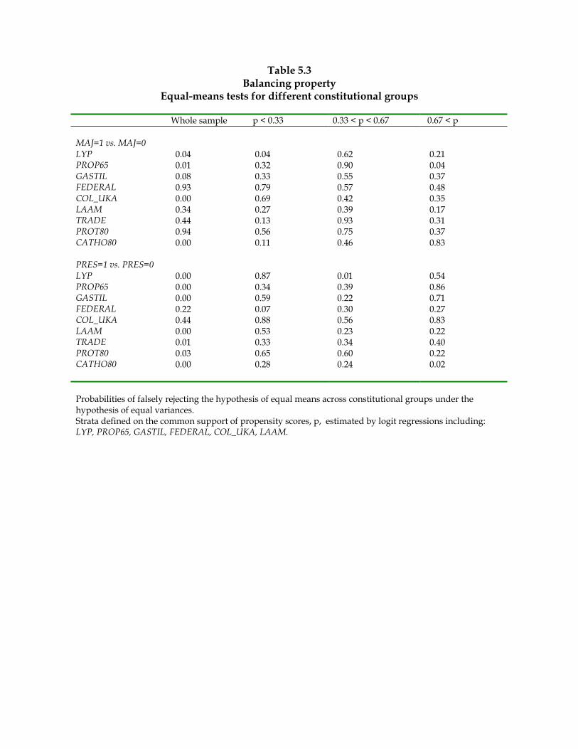
Table 5.3 Balancing property

Equal-means tests for different constitutional groups Whole sample p < 0.33 0.33 < p < 0.67 0.67 < p MAJ=1 vs. MAJ=0 LYP 0.04 0.04 0.62 0.21 PROP65 0.01 0.32 0.90 0.04 GASTIL 0.08 0.33 0.55 0.37 FEDERAL 0.93 0.79 0.57 0.48 COL_UKA 0.00 0.69 0.42 0.35 LAAM 0.34 0.27 0.39 0.17 TRADE 0.44 0.13 0.93 0.31 PROT80 0.94 0.56 0.75 0.37 CATHO80 0.00 0.11 0.46 0.83 PRES=1 vs. PRES=0 LYP 0.00 0.87 0.01 0.54 PROP65 0.00 0.34 0.39 0.86 GASTIL 0.00 0.59 0.22 0.71 FEDERAL 0.22 0.07 0.30 0.27 COL_UKA 0.44 0.88 0.56 0.83 LAAM 0.00 0.53 0.23 0.22 TRADE 0.01 0.33 0.34 0.40 PROT80 0.03 0.65 0.60 0.22 CATHO80 0.00 0.28 0.24 0.02 Probabilities of falsely rejecting the hypothesis of equal means across constitutional groups under the hypothesis of equal variances. Strata defined on the common support of propensity scores, p, estimated by logit regressions including: LYP, PROP65, GASTIL, FEDERAL, COL_UKA, LAAM.

Chapter 6

Fiscal Policy: Variation acrosscountries

6.1 Introduction

Armed with the methods introduced in the last chapter, we now proceed toestimating the constitutional effects on policy outcomes from cross-countrycomparisons. We mostly use the data from the 85 democracies in our ninetiescross-section. But when the data so permit, we also check the robustness ofthe results in cross sections based on our longer panel going back to 1960.In this chapter, we study fiscal policy, namely the size and composition ofgovernment spending and the budget surplus. The next chapter studies con-stitutional effects on political rents and productivity.Our goal is to estimate the effect of constitutional reforms, that is, chang-

ing the form of government or the electoral rule. The theories reviewed inChapter 2 suggest specific hypotheses about the effect of such reforms onfiscal policy. Switching from a parliamentary to a presidential form of gov-ernment is expected to reduce the size of government and, in particular,spending programs with many beneficiaries (such as general public goodsand broad welfare programs). The reason is that under a presidential regime,the majority of voters are not residual claimants on additional tax revenues.Spending is directed towards powerful minorities (rather than towards pro-grams benefiting many), and voters/tax payers can exploit the checks andbalances of a presidential regime to keep down overall government spending.No specific prediction has been formulated with regard to the budget deficit.

129

130CHAPTER 6. FISCAL POLICY: VARIATION ACROSS COUNTRIES

Switching from proportional to majoritarian electoral rule is also expectedto have significant effects on fiscal policy. The predicted effects are similar tothose of a switch to presidentialism, though the reasons are different. Manytheories predict that plurality rule and small electoral districts (i.e., majori-tarian elections) induce spending targeted to small, but pivotal, geographicconstituencies. Proportional elections instead induce political parties to seekconsensus in broad groups of the population and hence, naturally lead to pro-grams with many beneficiaries. Some theories also predict that majoritarianelections make it easier to limit both the size of government and the size ofbudget deficits. One reason (though not the only one) is related to the partystructure: majoritarian elections reduce the number of parties and the occur-rence of coalition governments which, in turn, helps resolving the commonpool problems that might be at the root of excessively large governments anddeficits.Throughout the chapter, we do not attempt to discriminate among dif-

ferent theories, nor do we consider the detailed mechanisms through whichthe constitution has an impact on policy outcomes. Instead, we estimate avariety of reduced forms, where the constitution is allowed to have a directeffect on the policy outcome of interest. Thus, we seek to quantify theseconstitutional effects, motivated by a set of theoretical priors, but withouttesting one specific model against another. Since this exercise is repeated fora variety of policy outcomes — in this chapter, as well as in the two following— our empirical results, in the end, paint a comprehensive picture which canbe fruitfully contrasted with the theoretical priors. However, we defer thisgeneral discussion to the last chapter of the book, after having seen all theresults.As discussed in Chapter 5, the effect of changing the form of government

and the electoral rule is estimated by the coefficients of the two binary in-dicator variables defined in Chapter 4: PRES and MAJ, respectively. Theestimated coefficient of PRES measures the constitutional effect of switchingfrom a parliamentary to a presidential system, holding constant the electoralrule and under the assumption that the electoral rule itself is of no impor-tance for this comparison (i.e., under the additivity assumption that theeffect of changing the form of government is the same whatever the rule forelecting the legislative assembly). Similarly, the estimated coefficient on thevariable MAJ measures the effect of switching from proportional or mixedto majoritarian electoral rule for the legislative assembly, holding constantthe form of government and under the assumption that the effect is the same


irrespective of the form of government.1 In some cases, we relax the additiv-ity assumption and allow interactions between constitutional reforms. Theconstitutional effects estimated under these more general assumptions cor-respond to the estimated coefficients of the dummy variables MAJPRES,PROPRES and MAJPAR, with proportional-parliamentary democraciesas the default group. The estimated coefficient ofMAJPRES thus measuresthe effect of changing both the electoral rule and the form of government atthe same time.Our empirical findings are discussed in different sections, each referring

to a specific fiscal policy outcome. In each section and for each policy out-come, we first estimate the constitutional effects by ordinary (linear) leastsquares. Then, we relax the conditional-independence assumption, using in-strumental variables and Heckman’s procedure. Finally, we relax the linearityassumption and estimate the constitutional effect non-parametrically, usingpropensity-score matching.Section 2 considers the size of government as measured by overall spend-

ing or revenue. We find presidential and majoritarian countries to have asmaller size of government, as expected. The effect of presidentialism isslightly larger and more robust. Both constitutional effects are weaker inthe earlier time period and stronger in the nineties cross section, therebysuggesting that presidential regimes and majoritarian elections have led tosmaller governments because they have dampened their growth in the post-war period.In Section 3, we evaluate the size of broad welfare-state programs. In this

case as well, we confirm our priors: presidential regimes and majoritarianelections have a negative effect on the size of welfare-state programs, butthese effects are weaker than for the overall size of government. Relaxingconditional independence and linearity suggests that the negative effect ofmajoritarian elections is the more stable result.Section 4 extends the analysis of constitutional effects to the budget bal-

ance. We find one very stable result across time periods and estimation

1As discussed in Chapter 4, majoritarian here refers to strictly majoritarian, while thealternative state (MAJ = 0) aggregates strictly proportional and mixed electoral rules.Allowing for a finer partition of the electoral rule, using our indicator for mixed electoralrules (MIXED), does not alter the results reported below while the estimated coefficientof MIXED is never statistically significant. This failure to discriminate between mixedand proportional systems might also reflect the relative scarcity of the mixed electoralsystems in our sample.


methods, confirming an earlier empirical finding in the literature: majori-tarian elections promote smaller deficits (or larger surpluses). The form ofgovernment has no stable causal effect on the propensity to run unbalancedbudgets, even though unconditionally, presidential regimes have larger sur-pluses than parliamentary regimes.Section 5 concludes by summarizing what we have learned from the evi-

dence. Overall, these empirical results are remarkably in line with the theo-retical priors, particularly in the case of the electoral rule.

6.2 Size of government

Does the constitution influence the size of government? To answer this ques-tion, we measure the size of government by central government spending andrevenue in percent of GDP (the variables CGEXP and CGREV introducedin Chapter 3). As discussed in Chapter 3, data on general governmentspending do not exist or are much less reliable. Nevertheless, when we applythe same methods to the smaller sample of countries where some data ongeneral government are available, the results are similar to those reportedbelow. Moreover, a dummy variable for federal countries (FEDERAL) isalways included in our basic set of control variables.

6.2.1 OLS estimates

We start by assuming conditional independence and linearity and estimatethe constitutional effects by OLS. The results are reported in Table 6.1.The most parsimonious specification, in column 1, relies on our nineties’cross-section. It holds constant variables that previous studies or a priorireasoning suggest to be correlated with the size of government spending. Asdiscussed in Chapters 3 and 4, we take these variables to be per capita in-come (LYH), openness (TRADE), two demographic measures (PROP1654and PROP65), the age and quality of democracy (AGE and GASTIL) anddummy variables for federal and OECD countries (FEDERAL and OECD).Being a presidential regime reduces the size of government by 6% of GDP.The point estimate is not only highly statistically significant, but also eco-nomically and politically so. Majoritarian elections also appear to producesmaller governments, but here the effect is smaller, about 3% of GDP, andless precisely estimated.

6.2. SIZE OF GOVERNMENT 133


The next column adds our indicator variables for geographical location(Africa, Asia and Latin America) and colonial origin (UK, Spanish, andOther, all discounted to the present from the date of independence). Asdiscussed in Chapters 4 and 5, these indicator variables are correlated withconstitution selection. Hence, the conditional independence assumption ismore credible in this more comprehensive specification. Only the dummyvariable for Latin America is significantly different from zero. But the esti-mated constitutional effect of presidential regimes is remarkably stable, theestimate dropping just slightly and maintaining about the same level of pre-cision. The estimated effect of majoritarian elections now exceeds 5% ofGDP. These results are quite robust to more parsimonious specifications ofthe continental dummy variables and the colonial origin variables, droppingone set of dummies but not the other, and to adding other controls such asincome inequality, a dummy variable for former socialist countries (not sta-tistically significant), or the age of democracy (AGE) entered both linearlyand squared (to allow for different function forms through which the age ofdemocracy influences policy outcomes).In column 3, we break down the constitutional variables into the finer

partition (MAJPRES, MAJPAR and PROPRES). The effects of thetwo constitutional features indeed appear to be additive, so that introducingboth a presidential form of government and majoritarian electoral rules in aproportional-parliamentary country would reduce the size of government bya whopping 10% of GDP.In column 4, we measure the size of government by revenue instead of

spending (the variable CGREV rather than CGEXP). The effect of presi-dential regimes is the same as before, but that of majoritarian elections isweaker. Later in the chapter, we shall see that the difference between govern-ment revenue and spending in majoritarian countries has a counterpart in ourresults for government deficits (which are consistently smaller in majoritariancountries).The 80 countries in our broad sample for the nineties (where all variables

are available) include some dubious democracies. In weak democracies, theformal constitution might play a less important role as compared to otherinformal practices and norms (we will return to a direct test of this idea,below). Moreover, some of the weaker democracies tend to be presidentialregimes, which might introduce a systematic bias. Column 5 thus restricts the


estimation to the better democracies in a narrower sample already discussedin Chapter 4 (62 countries for which GASTIL is smaller than 3.5). Theeffect of presidential regimes now appears to be even stronger, whereas thatof majoritarian elections remains stable and significant.

What happens when the average size of government is computed for alonger time period than the nineties? Column 6 reports on the same spec-ification as column 2, when the dependent variable is the average outcomeacross the 60 countries in our panel, starting in 1960. The effect of bothpresidentialism and majoritarian elections is still negative, but neither esti-mate is significantly different from zero. The weaker results do reflect thedifferent time period, rather than the different sampling of countries. Toshow this, column 7 in the table returns to the nineties’ cross section, re-stricting the sample to those countries included in the longer panel. Theseresults strongly suggest that the differences observed in the nineties’ datalargely result from a faster growth of government over the last forty yearsin countries with parliamentary regimes and proportional elections. We willreturn to this important theme in Chapter 8.

We have also searched for interaction effects between the constitutionand our covariates. In particular, we have tested whether the share of oldpeople, the quality of democracy and income inequality have the same effecton spending under different constitutions. We can reject the nul in the case ofincome inequality: larger inequality seems to produce a larger government —as expected from a simple median voter model — but only under majoritarianelections and presidential regimes. These estimates are fragile to the sampleand how inequality is measured, however, and thus, they are not emphasizedhere.

In summary, under the assumptions of conditional independence and lin-earity, the negative constitutional effect of presidential regimes is large (be-tween -5% and -8% of GDP) and robust to the specification. The electoralrule also has an effect on the size of government, associated with strictly ma-joritarian countries (a negative effect ranging from -3% to -6% of GDP). Botheffects conform to prior expectations. They are stronger in the later period,thereby suggesting that the constitution has influenced post-war growth inthe size of government.


6.2.2 IV and Heckman estimates

How robust are the above estimates of the constitutional effects when we tryto relax conditional independence? The short answer is that they are quiterobust.Consider first the Heckman procedure. As discussed in Chapters 4 and

5, in the first stage, we estimate by probit a constitution selection equa-tion specified as follows. One set of variables measures the date of origin ofthe current constitution: the three discretely measured indicators of constitu-tional origin (CON20, CON2150, CON5180) and the continuously measuredage of democracy (AGE). (Recall that the three indicator variables capturethe origin of the current constitution or the date of becoming a democracy,whatever came last.) A second set of variables measures the cultural influ-ence of the West, and Great Britain in particular. These are the distancefrom the equator (LAT01) — to measure different penetrations of coloniza-tion by the West — and the fraction of the population whose mother tongue isEnglish (ENGFRAC) or a European language (EURFRAC). Since manycountries in Latin America tend to be presidential systems with proportionallegislative elections, we also include a dummy variable for Latin America(LAAM). Finally, given the importance of British heritage to explain theelectoral rule, and since the fraction of the population speaking English isnot highly correlated with colonial origin, we also include a variable for UKcolonial origin (COL_UKA). These variables have considerable explanatorypower for both the form of government and the electoral rule — see Table 5.1in Chapter 5.The policy outcome equation (the second stage) is specified with the usual

set of regressors. To minimize the necessary adjustment for the correlationbetween unobserved determinants of constitution selection and performance,we also include dummy variables for colonial origin and continental location.2

The second-stage estimates for the Heckman procedure are reported incolumns 1 and 2 of Table 6.2. The estimated constitutional effects remainnegative and strongly significant. Allowing for an endogenous selection ofmajoritarian elections (column 2), the estimated correlation coefficient be-tween the random parts of constitution selection and performance (rho in thetable) is practically zero. Thus, the estimate is similar to the OLS estimates.When we allow for endogenous selection of presidential regimes (column 1),

2As noted in Chapter 5, we apply the Heckman correction to one constitutional dimen-sion at a time, treating the other dimension as random.


the correlation coefficient is instead positive and high: 0.64. Thus, the OLSestimates are likely to be upward-biased, and the Heckman correction pro-duces an even larger negative estimate of the constitutional effect. Theseresults are quite robust to alternative specifications of the first-stage equationfor constitution selection.


Next, consider instrumental-variable estimation. Here, we exploit thecrucial exclusion restriction that some variables entering the first stage donot influence fiscal policy, except through their effect on the constitution,once we hold constat other determinants of policy.We start with a parsimonious specification for both the first and the

second-stage regression. The second-stage regressors include our standardcontrols, but no continental and colonial indicator variables. The first stageis kept as in the Heckman estimation, except that we drop the dummy vari-able for Latin America (LAAM) and the variable for UK colonial origin(COL_UKA), i.e., the same specification as reported in Table 5.1 of Chap-ter 5. Thus, the identifying assumption is that the constitutional dating vari-ables (CON21, CON2150, CON5180), the language variables (ENGFRACandEURFRAC) and latitude (LAT01) are all uncorrelated with the remain-ing unobserved determinants of fiscal policy. The constitutional effects onthe size of government are reported in column 3 of Table 6.2.3 The pointestimates are similar to and — if anything — larger in absolute value than theOLS estimates of Table 6.1. They also closely correspond to those obtainedwith the Heckman correction in columns 1 and 2.Our identifying assumption says that any omitted variable is not corre-

lated with our instruments. For instance, if colonial origin or being in LatinAmerica influences the size of government, their effect would appear in theresidual of the second-stage equation (because they are omitted in column 3).This would not bias the IV estimates, however, as long as our instrumentsare not correlated with colonial origin or continental location. We consider

3Thus, among the second stage regressors, only AGE also enters in the first stage.This parsimonious first-stage specification is chosen to avoid excessively weak instruments.Imposing the restriction that only AGE plus the six instruments enter in the first stage,we estimate the first stage by OLS, run the second stage on the predicted values of MAJand PRES, and correct the second stage residuals as discussed by Maddala (1977, ch 11)and Wiggins (2000). The point estimates are very similar (or stronger) if all second-stagecontrols are added to the first-stage regression.


this a reasonable assumption in the case of the three dating variables, whilewe are less certain about the remaining three instruments. If we assume thefirst three instruments to be valid, however, the validity of the remainingthree can be tested via the implied over-identifying restrictions. As shown incolumn 3, we cannot reject the over-identifying assumptions, which reassuresus that the estimates are consistent, despite the omission of colonial originand continental location.Nevertheless, the power of the over-identification test might be low, since

the dating variables are only weakly correlated with constitution selection.Indeed, if we re-specify the first stage by omitting the more dubious in-struments (LAT01, ENGFRAC and EURFRAC), the fit of the first stagebecomes sufficiently weak for the estimated constitutional effects to be sta-tistically insignificant (though the point estimate remains negative and, inthe case of majoritarian elections, it is even larger in absolute value). Forthis reason, column 4 reports the results when we add the most likely cul-prits to the second stage, namely the variables for British colonial origin andLatin American location. The constitutional effect of presidential regimesnow drops towards its OLS estimate, but with a larger standard error, whilethe point estimate for majoritarian elections increases in absolute value, butremains statistically insignificant.4 One interpretation of these results is asfollows. A parsimonious first stage only leaves a small share of the variationin constitutional arrangements explained by the first-stage regressors. Thisvariation is insufficient to exert a significant influence on the size of gov-ernment, once we have also included all the dummy variables in the secondstage (since adding auxiliary controls keeps removing variation from the sizeof government).

6.2.3 Matching estimates

How robust are the results when we relax the assumption of linearity (butmaintain conditional independence), and estimate the constitutional effectsnon-parametrically with matching methods? As discussed at length in theprevious chapter, these quasi-experimental methods involve pairing up coun-

4The results are very similar if the first-stage regression associated with the estimatesin column 4 is expanded to also include the dummy variable for Latin America. Addingall the colonial origin and continental variables to the second stage, the standard errorsgrow even further.


tries with different actual constitutional rules, but similar estimated proba-bilities — propensity scores — of having selected a particular rule.The first step is thus to estimate these propensity scores for electoral rules

and government regimes, respectively. We have experimented with differentestimation methods for the selection equation: probit vs. logit. The dif-ferences are minor and we only display the results for the logit estimates.5

We have also tried different specifications of the variables entering these log-its. As explained in Chapter 5, our concern here is very different from thefirst-stage of the Heckman adjustment for self-selection. To respect condi-tional independence, we should include the most important determinants ofthe size of government, also correlated with constitutional selection. At thesame time, we should preserve some randomness in the selection process: ifwe explain constitutional selection too well, the common support becomesempty and the basis for matching is lost. We only report results for thenineties cross section, as we want to check whether the main results holdwhen relaxing the strong functional-form assumptions.We report the results for two different logit specifications. Both include

four potentially important determinants of the size of government, namelythe log of per capita income (LYP), the share of old people (PROP65),the quality of democracy (GASTIL), and the presence of a federal system(FEDERAL). In one specification, we also include the indicators for previ-ous British colonies and Latin American location, which correlate both withthe size of government and constitutional selection (adding other indicators,such as Spanish or Portuguese colonial origin is not feasible as we start per-fectly predicting some constitutional outcomes). The second specificationinstead adds the share of English and European language speaking people inthe population (ENGFRAC and EURFRAC), as well as latitude (LAT01).Table 6.3 displays the results. For each method of matching, we report

the estimates obtained under both logit specifications. The underlying stan-dard errors have been estimated by a bootstrapping procedure. The Kernelestimators (reported in columns 1 and 2) are the most reliable in a smallsample such as ours, while the nearest matching is the least reliable. As ex-plained in Chapter 5, in a small sample, measurement error or slight changesin the logit specification affect the ranking of countries based on the propen-

5Persson and Tabellini (2002) also report estimates of constitutional effects on the sizeof government with these same non parametric methods and a similar, but not identical,specification of the first (constitution selection) stage. The results are similar to thosereported below.


sity score. With the nearest matching estimator, this can have large impactson our estimates, while the Kernel estimator is more robust. With the firstlogit specification, and when imposing the common support restriction, wetypically discard 10 to 15 observations. The second logit formulation explainsthe constitution particularly well, and we end up losing more observations,particularly for presidential regimes where we are left with only 40 countriesin the sample of the common support of estimated propensity scores (seeChapter 5).


Despite these changes in the sample of countries and the estimation meth-ods, the estimates reported in Table 6.3 confirm the main message of theprevious subsections. Given the sample, the results are most directly com-parable to those in columns 1 and 2 of Table 6.1 and Table 6.2. Accordingto the more reliable estimates in columns 1-4 of Table 6.3, presidentialismreduces the size of government by between 6% and 8% of GDP, while ma-joritarian elections reduce it by between 4% and 6% of GDP. The nearestneighbor estimators dampen the effect of presidentialism and increase that ofmajoritarian elections. The standard errors of these estimates are larger thanthose of the OLS estimates, but that is to be expected as we are trading offless specification bias against higher standard errors in this non-parametricestimation. The most precise estimates are found by the Kernel estimator,which is intuitive as this method is the least sensitive to individual observa-tions.All in all, allowing for non-linear constitutional effects does not change

the conclusions we draw from these data.

6.2.4 Summary

The three sets of results paint a very consistent picture. If we are willing toassume conditional independence, given a large set of covariates, both con-stitutional effects are negative for the nineties’ cross section. Presidentialregimes and majoritarian elections each cut the size of government by about5% of GDP, perhaps more in the case of presidentialism. These results arerobust to relaxing the linearity assumption. Relaxing conditional indepen-dence does not change the estimated effect of majoritarian elections, whereasthe effect of presidential regimes appears to be even larger. The results for


presidential regimes conform with our theoretical prior, obtained from thework discussed in Chapter 2. In the case of majoritarian elections, our priorwas more fuzzy, but the empirical results lead us to revise it.

6.3 Composition of government

Do the constitutional effects extend to welfare-state spending? As discussedin Chapters 2 and 3, pensions and unemployment insurance are normally paidout in broad expenditure programs with many beneficiaries in the populationat large. This makes geographical targeting much harder than for other typesof discretionary spending, particularly in more developed countries. This iswhy, based on the theory, we expect the size of welfare spending to be smallerin presidential regimes and under majoritarian electoral rule. In this section,we investigate whether our main constitutional variables (PRES and MAJ )have direct or indirect effects on welfare-state spending, relying on the samebattery of methods as for the size of government.

6.3.1 OLS estimates

Table 6.4 reports on a variety of linear regression estimates. We hold constantthe same variables as in the standard specification for the size of government.On the whole, the estimated constitutional effects are smaller than for theoverall size of government. But the data reveal important interactions be-tween the constitution and other variables also influencing welfare spending.Column 1 refers to the full sample of countries in the nineties cross-section

(SSW, our measure of social transfers, is available for a dozen less countriesthan CGEXP, our measure of the size of government). Both presidentialregimes and majoritarian elections appear to reduce welfare-state spendingby about 2% of GDP, quite a large number. But neither effect is statisticallysignificant (p-values of 0.14 and 0.11). The results are similar in other (non-reported) specifications, such as when we drop the dummies for continentsand colonial origin, add income inequality, or the age of democracy squared.The absence of a strong constitutional effect may seem puzzling, given

that the size of welfare-state spending is (unconditionally) much smaller inpresidential and majoritarian countries — cf. Table 4.5 in Chapter 4. The keysocio-economic covariate driving the result is the proportion of elderly in thepopulation (as measured by PROP65). When this variable is held constant,

6.3. COMPOSITION OF GOVERNMENT 141

the estimated constitutional effects are about -2% of GDP in magnitude,but statistically insignificant; when the variable is omitted, these effects aremuch larger in absolute value and significant. In other words, presidentialand majoritarian countries do have smaller welfare spending on average but,in part, this reflects their younger populations.In column 2, the constitution is further subdivided into four separate

groups. As expected, switching both the electoral rule and the form ofgovernment is estimated to have the strongest effect (the point estimate ofthe dummy variable MAJPRES has the largest point estimate in absolutevalue). But only the estimated coefficient of the dummy variable PROPRES(corresponding to a change in the form of government in proportional coun-tries) is statistically significant.


As discussed in Chapter 5, constitutional features may shape policy out-comes with different strength at different stages of democracy. If such interac-tions exist, they may be particularly important here, as welfare-state spend-ing may be precisely triggered by broad political participation. Columns 3-5 of Table 6.4 show that the quality and age of a democracy indeed interactwith alternative constitutional features.In column 3, we confine the sample of countries to better democracies (56

countries where GASTIL is, on average, lower than 3.5 in the 1990s). Now,the estimated effect of a presidential regime is much stronger (over - 4% ofGDP) and significant, as predicted. The effect of majoritarian elections isalso stronger, but remains imprecisely estimated.6

Columns 4 and 5 return to the full sample of democracies, but interactthe electoral rule and the form of government with the age and quality ofdemocracy (measured by AGE and GASTIL). Variables PRES_OLD andMAJ_OLD in column 4 are defined as the product of PRES and AGE,and MAJ and AGE, respectively; the suffix OLD reminds us that highervalues of AGE correspond to older democracies. Similarly, the variablesPRES_BAD and MAJ_BAD in column 5 are defined as the product of

6These results on the electoral rule are weaker than the findings by Milesi-Ferretti,Perotti and Rostagno (2002), who estimate a negative and significant effect of less propor-tional electoral rules on social transfers in the OECD countries from 1960 to 1995 (theyneglect the form of government). Restricting the regressions for the longer cross section tothe 23 OECD countries in our sample (including the same covariates except the continentaland colonial-origin dummies), we obtain an insignificant effect close to zero, however.


PRES and GASTIL and MAJ and GASTIL, respectively, where the suf-fix BAD reminds us that higher values of GASTIL correspond to worsedemocracies.The estimates yield two results. First, and confirming the results in col-

umn 3, presidentialism and majoritarian elections restrain welfare spendingonly among older and better democracies (i.e., those with higher values ofAGE and lower values of GASTIL). We infer this from the negative esti-mated coefficients of PRES_OLD and MAJ_OLD in column 4, and thenegative estimated coefficients of PRES and MAJ in column 5, togetherwith the positive and significant estimated coefficients of PRES_BAD andMAJ_BAD.The significant estimated coefficients of variables AGE and GASTIL in

columns 4 and 5, respectively, also suggest a second inference. Older and bet-ter democracies (higher values of AGE and lower values of GASTIL) havesignificantly higher welfare-state spending only if they are parliamentary andproportional (the default constitutional state).7 This finding is consistentwith the common view among political scientists that proportional electionsand parliamentary systems allow for a better representation of disadvan-taged groups, that is, the likely beneficiaries of welfare-state spending. Inother words, these political institutions might better aggregate the policypreferences of disadvantaged groups into an actual influence on policy. Asdemocracies become older and allow for greater opportunities of politicalparticipation, the size of the welfare state increases. This effect of democ-ratization is only present in proportional and parliamentary democracies,however, and not among presidential and majoritarian democracies.8

What do the estimates tell us about the overall constitutional effect ofpresidential regimes or majoritarian elections, under the maintained assump-tion of conditional independence? In Chapter 5, we defined the constitutionaleffect as the average effect of constitutional reform in a country drawn at ran-dom, a definition that might also include interaction terms. Recalling the

7Summing the coefficients of AGE and PRES_OLD, we obtain a point estimate of1.06 with a standard error of 2.04 (transformed to take the linear combination of estimatedcoefficients into account). Thus, we cannot reject the nul hypothesis that the effect of AGEon welfare spending is zero among presidential regimes. The same results are obtained forthe set of majoritarian (parliamentary) countries, or for the effects of GASTIL.

8These interactions between the quality and age of democracy and the constitution areonly present when the dependent variable is welfare spending, and not in the case of theoverall size of government. This further supports the interpretation proposed in the text.


definition in equation (5.9), in column 5 we should add the estimated inter-cept (the coefficient on PRES or MAJ) to the estimated interaction effect(the coefficient on PRES_BAD or MAJ_BAD) times the average quality ofdemocracy (the average value of GASTIL) - or equivalently for the age ofdemocracy in column 4. These calculations for the estimates in columns 4and 5 produce a point estimate close to that in column 1 of Table 6.4, i.e.,both presidential regimes and majoritarian elections have lower welfare-statespending by about 2 % of GDP.Finally, in column 6 of Table 6.4 we interact our constitutional variables

with income inequality (measured by the Gini coefficient in the 1980s and1990s). One a priori reason for this to be interesting has already been men-tioned. The central prediction from the simple median-voter model — thatinequality boosts redistributive transfer payments — is most relevant whenelections have fewer candidates, which is more likely under majoritarian elec-tions or presidential forms of government. More inequality (higher values ofGINI) affects welfare spending in opposite directions under different forms ofgovernment. The significant negative coefficient on inequality (GINI) showsthat more inequality is associated with a smaller welfare state in parliamen-tary democracies, contrary to expectations and irrespective of the electoralrule (the estimated coefficient ofMAJ_GIN is close to zero). Since inequal-ity is measured in the 1980s and 1990s, while these welfare programs haveexisted in their current form for a longer time span, this might also reflectsome reverse causation (larger transfers might reduce inequality). In presi-dential regimes, inequality is instead associated with higher welfare spending(the sum of the coefficients on GINI and PRES_GIN is positive and signif-icant). Reverse causation might be less of a problem in Latin America (thehome of many presidential regimes), since those welfare programs are morerecent and more likely to target urban workers rather than the poor in thecountryside.Do the conditional results on the quality of democracy and income in-

equality reflect different mechanisms, or are they two sides of the same coin?After all, bad democracies are more likely to have higher income inequality(the simple correlation in our nineties cross section is 0.38). Furthermore,both variables are strongly correlated with presidential regimes (correlationcoefficients around 0.5). To answer this questions, we have allowed both in-teractions to appear simultaneously in the same specification. The results —not reported — are surprisingly stable, despite the relatively few degrees offreedom.


We have also estimated the same set of equations appearing in Table6.4 in the longer panel of 60 countries for which data are also availablefrom the early 1970s and onwards (unlike for the overall size of government,social security and other transfer data are not available for the 1960s). Allresults reported inTable 6.4 are very similar, including the interaction effects,suggesting that they are not a peculiarity of the 1990s.


Next, we relax the conditional-independence assumption, using instrumentalvariables and the Heckman two-step procedure in the broad nineties crosssection, where we have the largest number of countries. Despite the inter-action results just reported, we retain the restriction of a linear model withconstant slope coefficients. It would just be too demanding on the data toalso allow for endogenous constitution selection in this more complex spec-ification; moreover, we do not have reliable instruments for the quality ofdemocracy (as measured by GASTIL) or income inequality. Thus, the es-timates reported in Table 6.5 should be compared to the OLS estimates inTable 6.4, column 1.The specification of the first- and second-stage regressions for both the

Heckman and the instrumental variables estimates is identical to those forthe size of government.9 In particular, when we estimate by instrumentalvariables, we report two specifications for the second-stage estimates, oneinclusive of the dummy variables for British colonial origin and Latin America(column 4), the other not (column 3). Our previous concerns about thevalidity of the instruments remain, but are not repeated. Now, the over-identifying restrictions can indeed be rejected at the 10% level for the moreparsimonious second-stage specifications (column 3) and at the 5% level forthe less parsimonious ones. Recalling the interaction effects identified inthe previous subsection, the fragility of the Heckman correction to possiblefunctional form mis-specification is also an issue.


Despite these concerns, the pattern of the constitutional effects is con-sistent across the estimates reported in Table 6.5, while somewhat different

9Except in the first stage of the Heckman estimation when MAJ is treated as endoge-nous, where we drop the variable CON2150 to avoid a perfect prediction of 9 observations.


from the OLS estimates in Table 6.4 The presidential effect is not signifi-cantly different from zero. In the Heckman estimates, it is about the samesize as in the OLS regressions, namely about -2% of GDP (cf. column 1 ),consistent with the finding that the estimated correlation coefficient betweenthe unobserved determinants of constitution selection and performance (rho)is close to 0. In the instrumental variable estimates, it is practically zero.Overall, relaxing the conditional independence weakens the estimated effectof presidentialism.The effect of majoritarian elections, on the other hand, is reinforced. The

estimated coefficient of MAJ is now negative and statistically significantaccording to both procedures. Column 2 of Table 6.5 suggests errors witha strong positive correlation (a rho of +0.47), implying an upward bias inthe OLS estimate of the constitutional effect in Table 6.4. When the bias iscorrected, the constitutional effect of majoritarian elections becomes negativeand statistically significant (column 2), a result confirmed by each of theinstrumental-variable estimates (columns 3 and 4).The consistency of these results under two different estimation methods is

an indication that accounting for deviations from conditional independencemight be important. Once this has been done, there is stronger evidencethat majoritarian elections induce a smaller welfare state, while the form ofgovernment appears to be less important.


Finally, we turn to the matching methods and relax the assumption that thewelfare-state relation is linear in the covariates. In light of the interactionsreported in the OLS regressions, this extension seems quite important forassessing the robustness of our inferences. Once more, we proceed as for theoverall size of government by estimating two alternative logit specificationsof the propensity score — the same as already discussed for the size of govern-ment. The second specification entails a larger loss of countries, particularlywhen we estimate the presidential effect.


Table 6.6 displays the results for these specifications and our three match-ing methods. As noted in the previous section, the Kernel estimators are themost reliable in such a small sample. Despite the different estimators and


first-stage specifications for the propensity scores, most estimates are quitesimilar to those reported in Tables 6.4 and 6.5, if not larger in absolute value:both presidential regimes and majoritarian elections have a negative effecton welfare-state spending of about -2-3% of GDP, although the estimates arerarely statistically significant. As higher standard errors are to be expected,these consistently negative and stable estimates strengthen our belief thatboth constitutional effects are indeed negative, despite the interaction effectsdiscussed in connection with the OLS regressions.

6.3.4 Summary

Our findings suggest interesting constitutional effects on welfare-state spend-ing. Majoritarian elections cut welfare spending, as predicted by theory,and by as much as 2-3% of GDP. For presidential regimes the evidencepoints in the same direction, although the estimates are somewhat less ro-bust. Furthermore, there are interaction effects. Both constitutional effectsare much stronger among better and older democracies. Moreover, betterdemocracies have larger welfare states, but only if they are proportional-parliamentary. Selection bias seems to be a more severe problem here thanfor the size of government. Correcting for this reinforces the negative consti-tutional effect of majoritarian elections, but weakens the effect of the formof government.

6.4 Budget surplus

Is there a constitutional effect on government deficits? Earlier informal workand empirical results suggest that proportional electoral rules may be con-ducive to government debts and deficits, since they are often associated withunstable governments and coalition governments. Is this also the case in thebroad data sets used in this book? To investigate this question in a reduced-form manner, we apply the same approach as in the two earlier sections ofthe chapter, using the government surplus as a percentage of GDP (SPL) asour dependent variable.As noted in Chapters 3 and 4, a country cannot keep running a budget

deficit forever. The 1990s stand out as a somewhat special decade in thisrespect. Many countries began running large budget deficits in the 1970sand 1980s, while the 1990s was a period of budgetary consolidation, particu-

6.4. BUDGET SURPLUS 147

larly for some of the countries having accumulated large debts in the earlierdecades. To avoid basing our conclusions on data from a decade when severalcountries were trying to recover from large public debts, we only study the60-country panel for which we can take averages for the whole period 1960-1998. Most of the results reported below are very similar for the nineties’cross section, however.

6.4.1 OLS estimates

Columns 1-4 of Table 6.7 report the OLS estimates. Column 1 runs the samespecification as our basic regressions in the two previous sections. Countrieswith majoritarian elections have larger surpluses (smaller deficits) than thosewith proportional elections — the effect is precisely estimated and quite large,about 2% of GDP. Note that this regression includes a set of continentaldummies on top of our standard controls, so that the results do not reflect,say, larger deficits and a greater incidence of proportional countries in LatinAmerica. There is no significant effect of the government regime.


To address the possibility that larger or smaller deficits simply reflectinitial debt levels, in column 2 (and in all remaining columns in the Table),we also control for the level of debt in the first year when deficit data becomeavailable. The estimated coefficient on initial debt (not reported) is negativeand highly significant, meaning that a larger initial debt indeed leads toa smaller surplus, presumably because of higher interest payments.10 Themajoritarian effect only drops marginally, however, and remains significant.Similarly, the result is robust to excluding the worst democracies (column 4).Column 3 reports on the results from the finer disaggregation into four

constitutional states. Clearly, the main result in the other columns derivesfrom differences within the group of parliamentary countries. This gives someindirect support to the idea that coalition or minority governments — whichare much more common under proportional elections — may suffer from a

10Note, however, that in such cross-country regressions, the initial debt variable couldbe negatively correlated with the error term, thereby leading to a possible downward biasin the estimated debt coefficient (the dependent variable is the surplus).


status-quo bias or a dynamic common pool problem and find it harder to gettheir fiscal house in order, as compared to majority governments.Finally, as already noted in Chapter 3, we do not succeed in explaining

any considerable fraction of the cross-country variation in the surplus: theadjusted R2 is low, between 20 and 30%, despite the inclusion of dummyvariables for colonial origin and continental location. Other important de-terminants of budget deficits are unaccounted for by our standard controls.Nevertheless, the results are stable to alternative specifications or the sampleof the 1990s. Experiments with various interaction effects do not yield anystable results, but do not change the effect of majoritarian elections reportedabove.

6.4.2 Heckman estimates

The last two columns of Table 6.7 relax conditional dependence. Instrumental-variable estimation is problematic in the longer period 1960-1998: the vari-ables dating constitutional origin are no longer reliable instruments becausethe sample includes some constitutional reforms and countries becomingdemocracies for the first time (recall from Chapter 4 that the constitutional-origin instruments reflect the year when the constitutional feature was firstselected, or the year when the country became a ”democracy”, whatevercame last). Hence, these instruments should be more carefully redefined forthe longer period, which we have not done. Since we are only left with theless reliable instruments (LAT01, ENGFRAC and EURFRAC), we do notreport on instrumental variable results. For the same reason, the first stageof the Heckman model does not rely on the variables dating constitutionalorigin (the auxiliary instruments are less of a problem here, as we can stillachieve identification through the functional form assumption, as discussedin Chapter 5).Consider the constitutional effect of majoritarian elections (column 6 of

Table 6.7 ). The OLS estimates placed this around 2% of GDP (lower deficitsunder majoritarian elections). The Heckman procedure estimates the cor-relation coefficient between the unobserved parts of the electoral rule andperformance to be 0.28. This implies a small positive small bias in the OLSestimates; when this is corrected, the constitutional effect of majoritarianelections drop towards 1% of GDP and becomes statistically insignificant. Asimilar result is obtained for presidentialism (column 5), where the constitu-tional effect is now estimated to be very close to zero.

6.4. BUDGET SURPLUS 149

Overall, relaxing conditional independence suggests weaker constitutionaleffects. This result partly depends on the sample, however. In the crosssection of the 1990s (not reported), the constitutional effect of majoritarianelections remains about 2% and is statistically significant also according tothe Heckman estimates


As in earlier sections, we complement the parametric estimates of the consti-tutional effect with non-parametric estimates obtained by matching methods.Once again, the results rely on two logit specifications of the propensity scoreestimates. These are identical to the specifications for government size, ex-cept that we also include the initial debt level (CCG_NET_0 ). Table 6.8shows the results for these two specifications and our three matching meth-ods. In the case of presidential regimes, the second (more comprehensive)logit specification predicts too well in our smaller sample of 60 countries, andthe remaining observations on the common support are too few for reliableinference. Hence, for this second specification, we only report the estimatesof the constitutional effect for the electoral rule.


The estimates are most directly comparable to columns 2, 5 and 6 ofTable 6.7. Once again, majoritarian elections seem to promote larger sur-pluses (smaller deficits). The effect is estimated to be between 1% and 2%of GDP, though it is seldom statistically significant; as already noted, thisis not surprising with this non-parametric method. The estimated effect ofpresidential regimes fluctuates between being positive and negative, and isnever statistically significant.

6.4.4 Summary

All in all, our finding that majoritarian elections cause smaller governmentdeficits is quite robust to statistical pitfalls. The effect is also economicallylarge: about 2 % of GDP. No robust effect seems to be present when wecompare presidential versus parliamentary forms of government.


6.5 Concluding remarks

What have we learned about the differences between alternative electoralrules and alternative forms of government and their impact on fiscal policy?One important conclusion is that electoral rules exert a strong influence

on fiscal policy. Majoritarian elections induce smaller governments, smallerwelfare states and smaller deficits. These estimated constitutional effects arenot only statistically significant and robust. They are also quantitativelyrelevant. For a country drawn at random from our sample — and over a suffi-ciently long period to neglect transitory effects — a constitutional reform fromproportional to majoritarian elections reduces the size of central governmentspending by 4-5% of GDP, the size of welfare and social security programsby 2-3% of GDP, and the budget deficit by 1-2% of GDP.These findings are remarkably consistent with the qualitative predictions

of existing theory. As discussed in Chapter 2, there is not a single uni-fied theoretical model of how electoral rules shape fiscal policy. Differentauthors have emphasized different aspects and implications. But several ex-isting models predict that broad programs with many beneficiaries are largerunder proportional elections, and some also predict that proportional elec-tions are associated with larger overall spending and less disciplined fiscaland financial policies. The cross-country evidence uncovered here suggeststhese theoretical ideas to be on the right track. We have not attemptedto discriminate among alternative theories, however, nor have we sought toidentify the precise channel through which the electoral rule shapes fiscal pol-icy. Does the constitutional effect operate through the electoral incentives intwo-party electoral competition, as some recent theories have suggested? Oris the electoral rule of importance because it influences the party structureand thus, the incidence of coalition governments or the average duration ofgovernments? Discriminating among these alternative hypotheses is the nextimportant step in this research program.Turning to the form of government, our central empirical result is that

presidential regimes create considerably smaller governments than parlia-mentary regimes. A negative constitutional effect on welfare spending is alsopresent, but it is less robust. Once more, these constitutional effects arequantitatively large and about the same size as for the electoral rule. Areform from parliamentary to presidential regime would shrink the size ofoverall spending by about 5% of GDP, and the size of welfare programs byabout 2% of GDP. The effect on welfare spending is less precisely estimated,

6.5. CONCLUDING REMARKS 151

however, perhaps because many presidential regimes have younger popula-tions and it is difficult to separate the effect of the constitution from that ofdemographics in cross-country comparisons. These fiscal policy effects are inline with our theoretical priors, though here the theory of how the form ofgovernment shapes fiscal policy is less advanced than for the electoral rule.No effect of the form of government on budget deficits is apparent from thedata, nor did we expect to find one a priori.The robustness of some of these findings is remarkable, given the variety

of estimation techniques employed in this chapter. Cross-country compar-isons are often associated with ambiguous and fragile inference. We expectedthis to be particularly true in our case, given the non-random pattern of con-stitutional forms and the extensive differences among countries belonging todifferent constitutional groups. Nevertheless, when it comes to the broadfeatures of fiscal policy investigated in this chapter, the constitutional effectsdo seem robust to the most common econometric pitfalls in cross-sectionalanalysis. One reason might be that the unconditional differences in fiscalpolicy across constitutional groups are indeed very large. As pointed out inChapter 4, governments in parliamentary countries are about 11% of GDPlarger than in presidential countries; the unconditional difference betweenproportional and majoritarian countries amounts to about 5% of GDP. Theunconditional means in the other fiscal policy variables are also very differ-ent across constitutional groups. It is difficult to explain away such largedifferences on the basis of omitted variables, mis-specified functional forms,or other possible econometric pitfalls.Finally, these cross-country comparisons have revealed some interesting

interactions between the formal constitutional rules and the stages of democ-racy. The effect of the constitution on welfare spending is stronger in olderand better democracies. Conversely, older and better democracies are asso-ciated with larger welfare states, but only under parliamentary-proportionalconstitutions. This effect of the stage of democracy on policy outcomes, andits interaction with different constitutional rules, is a theme recurring alsoin the next chapter, where we focus on political rents and economic develop-ment. Although plausible ex post, we did not expect these findings on thebasis of existing theory. They deserve more attention in future research.

Table 6.1 Size of government and constitutions

Simple regression estimates

(1) (2) (3) (4) (5) (6) (7) Dep. var. CGEXP CGEXP CGEXP CGREV CGEXP CGEXP CGEXP PRES -6.08 -5.29 -5.17 -8.29 -3.46 -7.49 (1.97)*** (1.92)*** (2.44)** (2.72)*** (3.88) (2.72)*** MAJ -3.29 -5.74 -3.03 -5.59 -2.93 -4.81 (1.73)* (1.95)*** (1.85) (2.68)** (3.09) (2.75)* PROPRES -7.08 (2.70)** MAJPAR -7.30 (3.02)** MAJPRES -10.36 (2.70)*** Continent Yes Yes Yes Yes Yes Yes Yes Colonies No Yes Yes Yes Yes Yes Yes Sample 90s, broad 90s, broad 90s, broad 90s, broad 90s, narrow 60-90s, broad 90s,obs as(6) Obs. 80 80 80 76 62 60 60 Adj. R2 0.58 0.63 0.63 0.58 0.60 0.54 0.63

Robust standard errors in parentheses * significant at 10%; ** significant at 5%; *** significant at 1% All regressions include standard controls: LYP, GASTIL, AGE TRADE, PROP65, PROP1564, FEDERAL, OECD Narrow sample corresponds to countries where GASTIL is less than 3.5


Heckman and Instrumental Variables estimates

(1) (2) (3) (4) Dep. var. CGEXP CGEXP CGEXP CGEXP PRES -10.50 -5.37 -8.65 -4.50 (3.98)*** (2.19)** (3.63)** (3.89) MAJ -5.69 -4.92 -3.90 -5.12 (1.86)*** (2.57)* (3.46) (3.61) Conts & Cols Yes Yes No COL_UKA, LAAM Sample 90s, broad 90s, broad 90s, broad 90s, broad Endogenous selection

PRES MAJ PRES MAJ

PRES MAJ

Estimation Heckman 2-step

Heckman 2-step

2SLS 2SLS

rho 0.64 -0.02 Chi-2: over-id 4.64 3.61 Adj. R2 0.59 0.60 Obs. 75 75 75 75

Standard errors in parentheses * significant at 10%; ** significant at 5%; *** significant at 1%

Critical value of chi-2(4,0.05) = 9.49 Always included in second-stage specification (cols 1-4): AGE, LYP, TRADE, PROP1564, PROP65, GASTIL, FEDERAL, OECD First-stage specification of Heckman (cols 1-2) includes: CON2150, CON5180, CON81, AGE, ENGFRAC, EURFRAC, LAT01, LAAM First-stage specification of 2SLS (cols 3-4) includes: CON2150, CON5180, CON81, AGE, ENGFRAC, EURFRAC, LAT01


Matching estimates (1) (2) (3) (4) (5) (6) Dep. var. CGEXP CGEXP CGEXP CGEXP CGEXP CGEXP PRES -7.30 -7.91 -5.87 -7.92 -2.54 -4.00 (2.30)*** (2.90)*** (4.93) (5.11) (2.30) (3.45) MAJ -5.76 -6.55 -4.87 -4.08 -6.59 -8.81 (2.94)* (2.82)** (3.65) (4.16) (3.06)** (3.15)*** Estimation Kernel Kernel Strat Strat Nearest Nearest Sample 90s, broad 90s, broad 90s, broad 90s, broad 90s, broad 90s, broad Logit Specif.

1 2 1 2 1 2

Obs. on common support

65 PRES 67 MAJ

40 PRES 57 MAJ

65 PRES 67 MAJ

40 PRES 57 MAJ

65 PRES 67 MAJ

40 PRES 57 MAJ

Standard errors in parentheses obtained by bootstrapping * significant at 10%; ** significant at 5%; *** significant at 1% Kernel, Stratification and Nearest-neighbor estimators described in Chapter 5.5 Logit specifications underlying the propensity score estimates: 1: LYP, PROP65, GASTIL, FEDERAL, COL_UKA, LAAM 2: LYP, PROP65, GASTIL, FEDERAL, ENGFRAC, EURFRAC, LAT01

Table 6.4 Welfare spending and constitutions

Simple regression estimates (1) (2) (3) (5) (4) (6) Dep. var. SSW SSW SSW SSW SSW SSW PRES -1.89 -4.42 0.22 -8.65 -22.15 (1.27) (1.84)** (1.58) (2.94)*** (6.74)*** MAJ -2.01 -2.44 0.32 -4.96 -4.28 (1.25) (1.88) (1.60) (2.70)* (5.41) PROPRES -2.74 (1.58)* MAJPAR -2.72 (1.71) MAJPRES -3.51 (2.31) PRES_OLD -8.54 (3.81)** MAJ_OLD -7.69 (2.99)** AGE 1.14 1.51 1.16 9.60 3.62 -0.84 (2.60) (2.86) (3.60) (4.14)** (3.09) (2.90) PRES_BAD 2.67 (1.09)** MAJ_BAD 1.50 (0.86)* GASTIL -0.55 -0.61 -1.10 -0.67 -2.43 -1.39 (0.57) (0.56) (1.50) (0.58) (0.96)** (0.75)* PRES_GIN 0.57 (0.16)*** MAJ_GIN 0.06 (0.13) GINI_8090 -0.33 (0.12)*** Continents and Colonies


Sample 90s, broad 90s, broad

90s, narrow 90s, broad 90s, broad

90s, broad

Obs. 69 69 56 69 69 58 Adj. R2 0.75 0.75 0.73 0.78 0.78 0.81 Robust standard errors in parentheses * significant at 10%; ** significant at 5%; *** significant at 1% All regressions include standard controls: LYP, PROP65, PROP1564, GASTIL, AGE, TRADE, FEDERAL, OECD Narrow sample corresponds to countries where GASTIL is less than 3.5

Table 6.5

Welfare spending and constitutions Heckman and Instrumental Variables estimates

(1) (2) (3) (4) Dep var. SSW SSW SSW SSW PRES -1.99 -1.62 0.30 -0.39 (2.06) (1.37) (1.96) (2.34) MAJ -1.76 -3.21 -3.63 -4.13 (1.13) (1.64)** (1.82)** (2.12)* Continents and Colonies

Yes Yes No COL_UKA LAAM

Sample 90s, broad 90s broad 90s, broad 90s, broad Endogenous Selection

PRES MAJ PRES MAJ

PRES MAJ


Heckman 2-step

2SLS 2SLS

Rho 0.08 0.47 Chi-2: over-id 5.73* 9.81** Obs. 64 64 64 64 Adj. R2 0.78 0.78 Standard errors in parentheses * significant at 10%; ** significant at 5%; *** significant at 1% Critical value of chi2 (4,0.05) = 9.49 Always included in SSW equation: AGE, LYP, TRADE, PROP1564, PROP65, GASTIL, FEDERAL, OECD 2SLS first-stage specification includes: CON2150, CON5180, CON81, AGE, EURFRAC, ENGFRAC, LAT01 Heckman first-step probit specification includes: CON2150, CON5180, CON81, LAT01, ENGFRAC, EURFRAC, AGE, COL_UKA, LAAM (CON2150 dropped from probit for MAJ to avoid perfect predictions)

Table 6.6 Welfare spending and constitutions

Matching estimates (1) (2) (3) (4) (5) (6) Dep var. SSW SWW SSW SSW SSW SSW PRES -3.75 -3.11 -3.15 -1.83 -0.45 -2.02 (2.43) (1.89) (3.38) (2.78) (1.77) (1.54) MAJ -3.29 -4.62 -1.84 -1.89 -2.47 -3.70 (1.74)* (1.61)*** (1.92) (2.09) (1.96) (2.01)* Estimation Kernel Kernel Strat Strat Nearest Nearest Sample 90s, broad 90s, broad 90s, broad 90s, broad 90s, broad 90s, broad Logit Specif.

1 2 1 2 1 2


56 PRES 58 MAJ

35 PRES 50 MAJ

56 PRES 58 MAJ

35 PRES 50 MAJ

56 PRES 58 MAJ

35 PRES 50 MAJ

Standard errors in parentheses obtained by bootstrapping * significant at 10%; ** significant at 5%; *** significant at 1% Kernel, Stratification and Nearest-neighbor estimators described in Chapter 5.5 Logit specifications underlying the propensity score estimates: 1: LYP, PROP65, GASTIL, FEDERAL, COL_UKA, LAAM 2: LYP, PROP65, GASTIL, FEDERAL, ENGFRAC, EURFRAC, LAT01

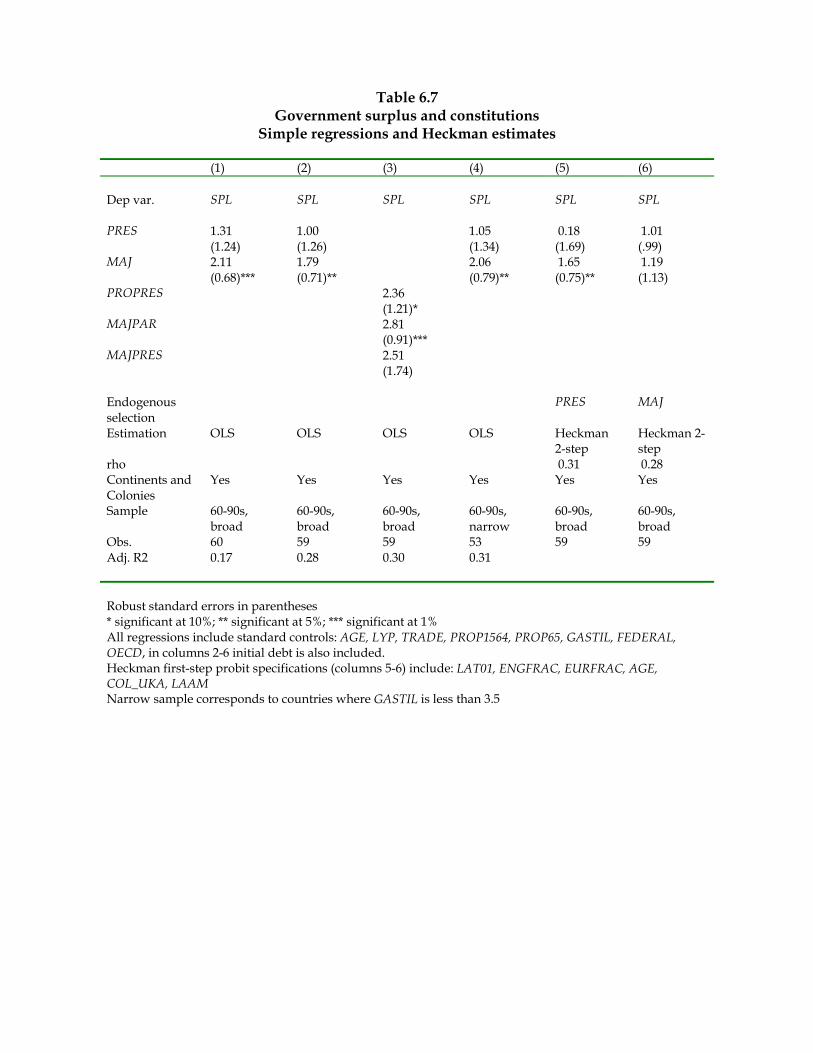
Table 6.7 Government surplus and constitutions

Simple regressions and Heckman estimates (1) (2) (3) (4) (5) (6) Dep var. SPL SPL SPL SPL SPL SPL PRES 1.31 1.00 1.05 0.18 1.01 (1.24) (1.26) (1.34) (1.69) (.99) MAJ 2.11 1.79 2.06 1.65 1.19 (0.68)*** (0.71)** (0.79)** (0.75)** (1.13) PROPRES 2.36 (1.21)* MAJPAR 2.81 (0.91)*** MAJPRES 2.51 (1.74) Endogenous selection

PRES MAJ

Estimation OLS OLS OLS OLS Heckman 2-step

Heckman 2-step

rho 0.31 0.28 Continents and Colonies


Sample 60-90s, broad

60-90s, broad

60-90s, broad

60-90s, narrow

60-90s, broad

60-90s, broad

Obs. 60 59 59 53 59 59 Adj. R2 0.17 0.28 0.30 0.31 Robust standard errors in parentheses * significant at 10%; ** significant at 5%; *** significant at 1% All regressions include standard controls: AGE, LYP, TRADE, PROP1564, PROP65, GASTIL, FEDERAL, OECD, in columns 2-6 initial debt is also included. Heckman first-step probit specifications (columns 5-6) include: LAT01, ENGFRAC, EURFRAC, AGE, COL_UKA, LAAM Narrow sample corresponds to countries where GASTIL is less than 3.5

Table 6.8 Budget surplus and constitutions

Matching estimates (1) (2) (3) (4) (5) (6) Dep. var. SPL SPL SPL SPL SPL SPL PRES -0.21 -0.26 0.20 (1.17) (1.43) (1.01) MAJ 1.16 0.78 1.80 1.12 2.11 1.91 (0.56)** (0.71) (0.76)** (1.28) (0.82)** (0.90)** Estimation Kernel Kernel Strat Strat Nearest Nearest Sample 60-90s, broad 60-90s, broad 60-90s, broad 60-90s, broad 60-90s, broad 60-90s, broad Logit Specif.

1 2 1 2 1 2


37 PRES 55 MAJ

44 MAJ

37 PRES 55 MAJ

44 MAJ

37 PRES 55 MAJ

44 MAJ

Standard errors in parentheses obtained by bootstrapping * significant at 10%; ** significant at 5%; *** significant at 1% Kernel, Stratification and Nearest-neighbor estimators described in Chapter 5.5 Logit specifications underlying the propensity score estimates: 1: LYP, PROP65, GASTIL, FEDERAL, COL_UKA, LAAM, CCG_NET_0 2: LYP, PROP65, GASTIL, FEDERAL, ENGFRAC, EURFRAC, LAT01, CCG_NET_0

Chapter 7

Political rents and productivity:Variation across countries

7.1 Introduction

In this chapter, we study the effect of the constitution on the size of politi-cal rents, on policies promoting economic development and economic devel-opment itself. As explained in Chapter 3, political rents are measured byperceptions of corruption and the abuse of power by public officials, and byperceptions of (in)effectiveness in the provision of public services. Economicdevelopment is measured by output per worker or total factor productivity,and policies towards development by a broad policy indicator of the pro-tection of property rights. Since these variables are only available in thesecond half of the nineties or, in the case of labor productivity and policiestowards development, in the mid 1980s, we confine the analysis to compar-isons in our nineties cross section.1 Throughout, we employ the same batteryof estimation methods as in the previous chapter’s study of fiscal policy.The theoretical work reviewed in Chapter 2 identifies several channels

through which the constitution can influence the incidence of corruption andthe abuse of power by public officials. Presidential regimes often have moreseparation of powers. Moreover, the executive is directly accountable to

1Our analysis of perceptions of corruption and the electoral rule draws on Persson,Tabellini and Trebbi (2002). That paper also studies a short panel of data on perceptionsof corruption for which yearly data are available from the mid 1980s until the late 1990s(the source is ICRG). The results of the panel-data study confirm the cross-sectionalfindings reported in this chapter.

153

154CHAPTER 7. POLITICALRENTSANDPRODUCTIVITY: VARIATIONACROSS C

voters and the dilution of responsibility often plaguing coalition governmentsis not an issue. On these grounds, the theory suggests lower rent extractionand less corruption under presidential regimes, as compared to parliamentaryforms of government.When it comes to the electoral rule, the predictions are more subtle. A

few papers on rent extraction have focused on the simple distinction betweenstrictly majoritarian and purely proportional electoral systems. Since theelection outcome is generally more sensitive to the incumbent’s performancein the former than in the latter, the prediction is that majoritarian electionsare more effective in deterring political rents. But other theoretical stud-ies have emphasized two details of electoral rules: the ballot structure andthe number of legislators elected in each district (i.e. district magnitude).Electing politicians from party lists (rather than individually) weakens theirincentives for good behavior, because it creates a free rider problem and amore indirect chain of delegation from voters to parties to politicians. Thus,ballots where voters directly choose individual incumbents are predicted toreduce the incidence of corruption, relative to those where citizens vote onparty lists. Smaller electoral districts raise higher barriers to entry, which ispredicted to increase corruption by reducing the choice set of voters. Withsmall districts, a smaller number of parties (or ideological types) are rep-resented in the legislature leaving voters with fewer alternatives to corruptpoliticians or parties. What do these detailed predictions imply for the sim-ple distinction between majoritarian and proportional elections? The answeris ambiguous, since the two effects tend to offset each other: proportionalelectoral systems typically combine large districts (which decreases corrup-tion) and party-list ballots (which increases corruption), while the oppositeis true under majoritarian elections (single-member districts with pluralityrule).In Section 2 of this chapter, we seek to discriminate between these dif-

ferent hypotheses. Presidential regimes are found to have less corruption, asexpected, but this is a fragile result: it only appears among better democra-cies or if we relax conditional independence. Turning to the electoral rule,we find that what is of importance are the details, not the raw distinctionbetween majoritarian and proportional systems. Large districts and vot-ing over individuals both reduce corruption, as expected. But corruptionis roughly the same when we compare across our broad classification intoproportional vs. majoritarian systems. Evidently, the opposite effects of theballot structure and district magnitude offset each other, with no robust net


effect.The rest of the chapter tries to identify the effect of the constitution on

two ultimate measures of good economic performance, namely labor and totalfactor productivity. As discussed in Chapter 3, previous studies have foundproductivity to be well explained by a broad policy indicator of protectionof property rights and anti-diversion policies (the variable GADP ). Here,we ask whether electoral rules or forms of government have an effect onproductivity, directly or through this broad policy indicator.A priori, the constitution could influence productivity and policies to-

wards development in several ways. Naturally, one channel is corruption.Whenever corruption redistributes rents from producers to politicians, ithurts economic development. Hence, any constitutional feature with an im-pact on corruption is also likely to influence productivity. This suggests thatpresidentialism, large electoral districts and ballots for individuals should beassociated with better economic policies and higher productivity. There areother possible offsetting channels, however. Small governments and low taxdistortions in presidential and majoritarian political systems could inducehigh productivity, by high investment. But, as discussed in Chapters 2 and6, the same constitutional features could also lead to targeted redistributionand low public-good provision. Such policies are likely to involve poor generalprotection of property rights, and distortions in the allocation of economicactivity, with negative effects on productivity. Overall, the constitutionaleffects on productivity and policies towards development have an ambiguoussign. Hence, our empirical work in this chapter is really more of a preliminarysearch for interesting patterns in the data, than a test of specific hypotheses.In that search, we also ask what is the link between productivity and

the age of democracy (as measured by AGE). This variable could also influ-ence performance in two opposite ways. On the one hand, older democraticinstitutions might perform better, as citizens will have learned to use themeffectively in fighting government abuse and corruption. Indeed, a recentempirical “event study” by Roll and Talbott (2002) shows economic growthtaking off, once a country becomes democratic. On the other hand, accordingto Olson (1982), older and more stable democracies are more easily capturedby organized special interests, which might hurt their long-run economic per-formance.Our empirical results on economic performance are reported in Section 3.

Majoritarian elections at large do not have a robust causal effect on policy orproductivity, but the finer details of the electoral system do: voting over indi-


viduals and large district magnitude promote productivity-enhancing policyin much the same way as they deter rent extraction. We also find parliamen-tary regimes and older democracies to select better policies towards economicdevelopment and for this reason, they have higher productivity. But our re-sults also indicate that this negative effect of presidentialism on productivityis mainly due to the worse democracies in our sample. Combining these re-sults with those on corruption, we tentatively conclude that presidentialismreduces rent extraction under better democratic conditions, while it hurtseconomic performance under worse democratic conditions.Section 4 summarizes and contains some concluding remarks.

7.2 Political rents

As discussed in Chapter 3, we gauge political rents by three alternative mea-sures concerning perceptions of rent extraction. Two of these refer to theperception of corruption by public officials (GRAFT and CPI9500), thethird to (in)effectiveness in the provision of government services (GOV EF ).As we have most observations for GRAFT, and this variable is probably mostclosely related to the theoretical construct of political rents, we mainly focuson this indicator. But we show that the results also extend to the other mea-sures. Our goal in this section is to describe how alternative constitutionalfeatures influence these perceptions of rent extraction.The form of government is measured by our binary indicator for presi-

dentialism, PRES. The simple distinction between majoritarian and propor-tional or mixed electoral systems is measured by the binary variable MAJ .In this chapter, we also measure more detailed aspects of the electoral rule,however. The continuous variable MAGN is a measure of inverse averagedistrict magnitude (see Chapter 4). It captures the barriers to entry in theelectoral race, as it assigns higher values to fewer candidates elected per dis-trict, and we expect it to induce more corruption. The continuous variablePIND is a measure of the percentage of legislators not elected from partylists (again, Chapter 4 gives an exact definition). Thus, it is predicted toinduce less corruption..We follow the same empirical strategy as in the previous chapter: first

we estimate some simple regressions, then we relax conditional independenceand finally we relax linearity. The more general estimation methods onlyapply to the effects of the binary constitutional variables (MAJ and PRES),

7.2. POLITICAL RENTS 157

however. Hence the analysis of how the details of the electoral rule influencerent extraction is confined to the simple linear regressions reported in thenext subsection.

7.2.1 OLS estimates

Table 7.1 reports on the results of simple regressions, estimated under theassumptions of linearity and conditional independence. To help reduce thenoise from measurement error, the estimation method is always weightedleast squares, where the weights are given by the (inverse) standard deviationof the dependent variable (see Chapter 3 for more details). Estimating byOLS and correcting the standard errors for heteroscedasticty, produce verysimilar results. Throughout, we hold constant a dozen variables that otherstudies have found to influence the perception of corruption, such as percapita income, religious beliefs, education, and so on (see Chapter 3 fordiscussion and references, and the notes to Table 7.1 for a complete listof the controls). We also hold constant continental location and colonialorigin. Controlling for legal origin instead of colonial origin leads to similaror stronger estimated constitutional effects, meaning that we report the leastfavorable specification for the theory.Consider first the effect of the form of government. In column 1, rent ex-

traction is measured by GRAFT, while the constitutional features are mea-sured by the binary variable for presidentialism (PRES) and the continuousmeasures for the electoral rule (PIND and MAGN). Presidentialism has anegative estimated effect on rent extraction, as expected. But its estimatedcoefficient is only significant at the 10% level, and small in absolute value(recall that all our measures of corruption vary from 0 to 10). Neglectingcolumns 2 and 3 for a moment, the estimated coefficient of presidentialismis insignificant in all the other columns of Table 7.1, where rent extraction ismeasured by the other two perception variables, CPI9500 and GOV EF , orthe electoral rule is measured by other indicators such as PROPN, PDM orMAJ.A possible interpretation of this inconclusive finding on the form of gov-

ernment is that our measure of presidentialism does not square well with thetheory. As discussed in Chapter 4, our distinction between different forms ofgovernment relies on the confidence requirement, and not on the separationof powers. Yet, according to the theories reviewed in Chapter 2, presidentialgovernments mainly reduce political rents because of their greater separation


of powers than parliamentary governments.But columns 2 and 3 suggest another possibility: an interaction between

the form of government and the quality of democracy. Presidential regimesare often found in worse and younger democracies, where the formal consti-tutional rules might be less important and the stronger checks and balancesassociated with presidentialism might not exert their full effect. Indeed, asshown in column 2, presidentialism has a negative and significant effect oncorruption, once we restrict the sample to better democracies. In column 3,we interact the PRES indicator with the quality of democracy (as measuredby GASTIL) in the full sample. The estimated coefficient of presidentialismincreases further and acquires a stronger statistical significance, but its ef-fect is dampened in worse democracies (recall that higher values of GASTILcorrespond to worse democracies).A third possibility is a combination of the other two. It may be that

separation of powers is lacking precisely in the worst democracies. Indeed, asdiscussed in Chapter 4, the GASTIL measure partly reflects whether thereare effective checks on the behavior of the executive.


Next, consider the effect of electoral rules. Here, the data strongly supportthe idea of the details of the electoral rule being important determinants ofrent extraction. As shown in the first two columns of Table 7.1, inversedistrict magnitude and ballots with individuals are statistically significantwith the expected sign: more individual voting (higher values of PIND)reduces corruption, while higher barriers to entry associated with smallerdistricts (higher values of MAGN) increase corruption. This result is robustto the sample of better democracies (i.e. those with a GASTIL score smallerthan 3.5, in column 2). Moreover, the estimated coefficients of PIND andMAGN are large (both variables are defined so that they lie between 0 and1) and their standardized beta coefficients are, by far, the largest of all theregressors. For example, switching from a system where all legislators areelected on party lists (PIND = 0), to one where all are elected as individuals(PIND = 1), is estimated to reduce the perceptions of corruption by wellover 20% (2 points out of 10) in the sample of good democracies, which isabout twice the effect of not being a Latin American country. The estimatedeffect of inverse district magnitude (also taking positive values below 1) iseven larger, though it is somewhat less stable to the specification. Omitting


the dummy variables for continental location and colonial origin does notimportantly affect the coefficient of PIND, though the coefficient ofMAGNbecomes somewhat smaller and remains statistically significant only at the10% level. Finally, these variables are not only individually, but also jointly,significant. Given the high correlation between these two variables and theiropposite effect on corruption, this is a further sign that we are not just pickingup a statistical artifact.Being a survey of surveys, the dependent variable is clearly measured with

error. This is the rationale for our WLS estimation, attaching lower weightsto observations where the different components of the perception index aremore divergent. In columns 4-6 of Table 7.1, we carry out additional sensitiv-ity analyses, with alternative measures for our dependent and independentvariables. Columns 4 and 5 report on the same specification as in column 1,but with either GOVEF or CPI9500 as the dependent variable. The resultsare even stronger when we measure corruption by CPI9500 and almost asstrong when we instead consider GOVEF, measuring ineffectiveness in gov-ernment (recall from the previous section that we have re-scaled all thesemeasures to run on a scale from 0 to 10). Column 6 replaces our own twomeasures of the electoral system by the alternatives from the data set con-structed by Seddon et al (2001) and defined in Chapter 4. Recall that PDMis their measure of district size, defined so that higher values mean largerdistricts, not smaller as with our variableMAGN. Similarly, PPROPN, theirmeasure of legislators elected at the national level, is an inverted measure ofindividual accountability, and not a direct measure as our PIND variable.Thus, the expected sign of these two variables is the opposite relative toPIND and MAGN. As shown in column 6, the main results hold up equallywell with these alternative measures.Overall, these simple regressions strongly suggest that the details of the

electoral rules influence corruption, as expected. Countries predominantlyvoting over individuals tend to have less corruption than those predomi-nantly voting over parties. Countries with smaller electoral districts alsotend to have more corruption. According to these results, a comprehensiveelectoral reform, going from a Dutch-style electoral system with party lists ina single national constituency to a UK-style system with first past the postin one-member districts (i.e., moving both MAGN and PIND from approxi-mately 0 to 1), would have two counteracting effects on corruption, producinga net result close to zero. A better reform from the viewpoint of reducingrent extraction would be to switch to plurality rule voting for individuals, but


keeping districts with more than one member as in Chile (two-member dis-tricts and MAGN = 0.5) or Mauritius (three-member districts and MAGN= 0.33). Indeed, these countries, especially Chile, turn out to have very lowcorruption levels as compared to neighboring countries.Another way of asking what are the effects of a comprehensive electoral re-

form from proportional to majoritarian elections is to infer the constitutionaleffect of the estimated coefficient of our binary indicator for the electoral rule,MAJ. This question is of independent interest, since according to some mod-els reviewed in Chapter 2, majoritarian electoral systems enhance electoralaccountability and thus, deter corruption. The result is shown in column 7of Table 7.1. The estimated MAJ coefficient is negative, but small and sta-tistically insignificant. The estimated MAJ coefficient increases somewhatin absolute value, and becomes marginally significant if we do not control forcolonial origin (results not reported). As noted in Chapter 4, majoritarianelectoral rules are often found in former British colonies, and it is difficult totell the influence of these two variables apart (when we control for continentsor legal origin, the constitutional effect remains negative and statisticallysignificant, so it is really colonial origin that makes a difference). But tointerpret the estimate of a regression that does not control for British colo-nial origin as a causal constitutional effect, we would need to assume colonialorigin not to have any effect on perceptions of corruption, which is not veryplausible.


We only attempt to relax conditional independence for the binary constitu-tional indicators (MAJ and PRES). In principle, the continuous measuresof the electoral rules (such as PIND and MAGN) might also be correlatedwith the random component of rent extraction, which would bias the OLSestimates. But the Heckman procedure cannot be applied to continuous vari-ables. Instrumental-variable estimates are also problematic, because our in-struments for constitutional origin are unlikely to be appropriate. The finermeasures of the electoral system change more frequently than the simplerclassification into majoritarian and presidential constitutions, so it would bemore difficult to date them back to specific historical periods. Thus, in thissection, we only apply instrumental variable estimation and the Heckmanprocedure only to the binary variables MAJ and PRES.With our standard specification (colonies and continents included in the


second stage), the two-step Heckman procedures yield estimates of the cor-relation coefficient (rho) of +1 or -1, thereby suggesting a perfect correlationbetween the error terms between constitution selection and performance.As this is implausible, we instead preform the Heckman correction with amaximum-likelihood estimator. To achieve convergence of the maximiza-tion algorithm, however, we must impose more parsimonious first-step andsecond-step specifications for both constitutional variables, as compared tothe specification adopted in Chapter 6. Specifically, when estimating thefirst-step (probit) regressions, we drop the indicator variables for consti-tutional origin (CON2150, CON5180 and CON81); the remainder of thespecification is as in Chapter 6 (see also the discussion in Chapter 5). Inthe second step, we only include the dummy variables for UK colonial originand Latin America, besides all the standard controls, thus omitting the othercontinental and colonial origin indicators.Instrumental-variable estimation is also performed in a slightly different

way, compared to Chapter 6. Our instruments are still the same as thosediscussed in Chapter 5 and used in Chapter 6: the three indicators for con-stitutional origin (CON2150, CON5180 and CON81), latitude (LAT01)and the fractions of the population whose mother tongue is English or a Eu-ropean language (ENGFRAC and EURFRAC). But here, we move in theopposite direction and adopt a less parsimonious first stage specification thanin Chapter 6: we now run the first-stage regression of the 2SLS estimates onthe full set of the six instruments plus all controls entering the second-stageregression (see Table 7.2 for a complete list). Several of the second-stagecontrols now measure historical and social variables, such as religious beliefsor ethnic fractionalization, which could also influence constitution selection.Excluding such controls from the first stage, if they belong there, might biasthe 2SLS estimates of the constitutional effect. Furthermore, adding the fullset of controls to the first stage now increases the explanatory power of thedummy variables dating constitutional origin, and thus reduces our concernfor weak instruments.2 For both these reasons, the inference is more reliablewith a less parsimonious first-stage specification.


2The F tests of the nul hypothesis that all instruments dating constitutional originhave a zero coefficient in the first-stage regressions for presidentialism and majoritarianelections yield the test statistics F = 3.06 ** and F = 2.26* , respectively.


Consider the constitutional effect for presidentialism. The Heckman pro-cedure (column 1) produces a positive and highly significant estimate (rho =0.57) of the correlation between selection of a presidential regime and cor-ruption. Correcting the upward bias in the OLS estimates, the constitutionaleffect is a reduction in corruption/rent extraction by about 1 point (out of10), a statistically significant and non-trivial effect. The 2SLS estimates(column 3) yield the same result, namely a large and statistically significanteffect of presidentialism on corruption. The fact that both estimators pro-duce similar results, despite the different identification assumptions, suggeststhat a violation of conditional independence could indeed bias the OLS esti-mates towards zero. As shown by columns 4 and 5, there is a negative effectwhen we replace GRAFT by the two alternative measures of rent extraction.For majoritarian elections, we reach the opposite conclusion. The esti-

mated correlation coefficient in column 2 is negative (rho = −0.47), thoughimprecisely estimated, and the constitutional effect is now positive, althoughinsignificant (i.e., a sign reversal relative to the OLS estimates). Once more,the instrumental variable estimation in columns 3-5 reinforces this conclu-sion.Thus, addressing conditional independence does make a difference in the

case of corruption. The OLS estimates suggested no effect (or a negative butsmall and fragile effect) of government regimes and majoritarian electionson corruption. The conclusion regarding the form of government is reversedwhen allowing for conditional independence. Presidential regimes are foundto reduce corruption, while for majoritarian elections, the inference of noconstitutional effect is reinforced.


We end with the non-parametric estimates, re-imposing the conditional inde-pendence assumption. Because the matching methodology requires a binaryvariable, we only report results for the two simple constitutional indicators(MAJ and PRES). Columns 1 to 3 of Table 6.14 show the constitutional ef-fects on rent extraction measured by GRAFT, according to our three match-ing estimators. The specification of the propensity score includes a basicset of six covariates (LYP, GASTIL, AVELF, PROT80, COL_UKA andLAAM ). In columns 4 and 5, GRAFT is replaced by the two alternativemeasures (CPI9500 and GOVEF ), for the same logit specification and theKernel estimator. Column 6, finally, maintains GRAFT as the dependent

7.3. PRODUCTIVITY 163

variable, but relies on a different propensity-score specification.


The results can be stated briefly. The presidential effect now becomespositive, though always statistically insignificant and small. The effect ofmajoritarian elections is always negative, but never significant. Neither es-timate is very stable, and in other (non reported) specifications, the sign ofboth effects changes, though always remaining small and insignificant. Over-all, these estimates suggest that neither constitutional feature has a robusteffect on corruption. Our conjecture that the linear OLS estimates of thepresidential effect were hiding a potentially relevant interaction between theform of government and the quality of democracy does not seem supported bythis more general estimation method which allows for non-linear functionalforms. Note, however, that we do impose conditional independence.

7.2.4 Summary

The overall picture emerging from this section is multi-dimensional. Presi-dential regimes do not have a stable effect on political rents under the main-tained assumption of conditional independence (required by OLS and match-ing), except in better democracies. Relaxing conditional independence seemsempirically important and produces a negative constitutional effect, however.What about the electoral rule? Here, the central empirical result is that

the devil is in the details. Larger electoral districts seem to cut rent extrac-tion, as do elections where voters cast their ballots for individual politiciansrather than party lists. From the perspective of a radical reform from pro-portional to majoritarian elections, these two aspects of the electoral systemtend to offset each other, with no net effect on corruption; a result confirmedby the estimates associated with our binary indicator for plurality rule.

7.3 Productivity

In this section, we search for constitutional effects on two ultimate measuresof economic performance, namely labor productivity, i.e., output per worker(LOGY L), and total factor productivity (LOGA). The main difference be-tween these two is that labor productivity largely reflects underlying capital


intensity and thus previous capital accumulation, whereas total factor pro-ductivity does not. We first estimate a direct constitutional effect on thesetwo variables, by a reduced form similar to that in the existing literatureon cross-country productivity differences. It is important to probe furtherbeyond any reduced-form findings, however. Specifically, do our constitu-tional variables explain a broad policy indicator of protection of propertyrights and anti-diversion policies (GADP ) that previous studies have foundto be an important determinant of productivity? (See Chapter 3 and Halland Jones (1999) for a precise definition and discussion.) Do such indirectconstitutional effects on productivity operate through the policies studiedearlier in this chapter and the previous one, namely the size and compo-sition of government spending or corruption? Are higher productivity andbetter economic policies related to the age of democracy. Are the estimatesrobust to endogenous selection of the constitution, and non-linearities in theoutcome relation?

7.3.1 Reduced-form estimates

We begin by estimating a simple reduced form by OLS, with the two produc-tivity measures as our dependent variables. The underlying specification isthe same as in Chapter 3 which, in turn, follows Hall and Jones (1999) closely.Thus, we control for latitude (LAT01), the fractions of the population speak-ing English or a European language (ENGFRAC and EURFRAC), a mea-sure of comparative advantage in international trade (FRANKROM) andour indicator for federalism (FEDERAL). But now, we also add our usualconstitutional variables plus the age of democracy (AGE) to the regressors.We always hold constant continental location and colonial origin to lend morecredibility to the conditional-independence assumption (omitting these indi-cator variables, we obtain stronger estimated constitutional effects, with thesame signs as those described below).Columns 1 and 2 of Table 7.4 show that both presidential regimes and

majoritarian elections have a negative coefficient: according to these reduced-form estimates, both constitutional features harm economic performance.The effect on total factor productivity is smaller and not statistically signifi-cant, suggesting that the negative effects might operate through disincentivesfor capital deepening (i.e., investments in physical or human capital). Totalfactor productivity is also harder to explain — the regression in column 2 ex-plains about 50% of the variation in productivity, as opposed to about 70%


in column 1 — probably because of larger measurement error. To gauge thesize of the constitutional effect, recall that labor productivity is expressed inlogs and ranges from a maximum of about 10.5 for the US to a minimumof about 7 for Malawi. According to the estimates in column 1, switchingfrom parliamentarism to presidentialism or from proportional to majoritarianelections reduces labor productivity by about 0.3: a non-trivial effect closeto the difference between the US and the UK, or between Spain and Greece,in the mid 1980s.Columns 3 and 4 decompose the effect of the electoral rule in the same

two dimensions as in the previous section, namely the fractions of legisla-tors elected with an individual vote (PIND) and (the inverse of) districtmagnitude (MAGN). Our previous results for rent extraction lead us toexpect positive and negative effects on productivity, respectively, from thesevariables. These signs are indeed what we find. Moreover, the estimatedcoefficients are statistically significant and quite large. In these regressions,however, the effect of the form of government seems to vanish.


The constitutional effect on labor productivity of presidential regimesand majoritarian elections is sensitive to the sample of countries: a signifi-cant estimate is obtained in the broader sample, but not among the betterdemocracies (column 5). This fragility does not extend to the finer measuresof the electoral system (PIND and MAGN), however, which remain sta-tistically significant when we restrict the sample to the better democracies(column 6). In the case of total-factor productivity, none of the constitu-tional variables is statistically significant in the narrow sample, and the fitof the regression is generally rather poor.As shown in all columns of the table, the age of democracy (AGE) is

strongly correlated with economic performance. Older democracies are moreproductive, and the effect is statistically significant for all measures of pro-ductivity, all specifications, and almost all samples.These reduced-form estimates indicate some intriguing constitutional ef-

fects on productivity, over and beyond the historical, geographical and cul-tural variables held constant in these regressions. Presidential and majoritar-ian countries seem to have lower productivity, particularly in worse democra-cies, and the specific form of the electoral system also seems to be of impor-tance. To gain more insights into the channels of these constitutional effects,


we need to estimate a more structural model, which maps our constitutionalmeasures into observable policies, and these policies into productivity. Thenext subsection attempts to make some progress on this non-trivial task.

7.3.2 Structural-form estimates

Do the constitutional effects on productivity operate exclusively throughthe comprehensive policy indicator of anti-diversion policies (GADP )? Thisquestion consists of two parts: (i) is there a constitutional effect on this broadpolicy indicator? (ii) are there direct constitutional effects not going throughthis indicator, thus reflecting some other policy channels?3

Column 1 of Table 7.5 addresses sub-question (i) by OLS estimation (re-taining the assumption of conditional independence) and a specification fol-lowing the reduced form of Table 7.4. Thus, we control for the age of democ-racy, our indicators for federalism, colonial origin and continental location,plus the four Hall-Jones variables mentioned above. Recall that higher val-ues of the policy indicator (GADP ) amount to better policies, and that thevalues range from about 0.3 (for Bangladesh) to 1 (for Switzerland). As ex-pected from the reduced-form estimates, parliamentary regimes have betterpolicies with quite a substantial effect. The age of democracy is also statis-tically significant, with older democracies having much better policies. Butnow, the broad form of the electoral rule does not seem to be of importance.


Next, we ask whether the anti-diversion policy indicator has an effecton productivity. The estimation is by 2SLS, where policy is endogenized inthe first stage with the specification underlying column 1. The second-stageproductivity equations reported in columns 2 and 3 still include the colonial-origin and continental variables, but nothing else. Thus, the instrumentsfor GADP are the same as those used by Hall and Jones (1999), plus ourfour constitutional variables: the dummy variables for presidentialism, ma-joritarian elections, federalism, and the age of democracy. The identifying

3As discussed in Chapter 3, Hall and Jones (1999) argue that two policy variables couldaccount for cross-country differences in productivity. One is the indicator of anti-diversionpolicies (GADP ), the other an indicator of commercial policy (Y RSOPEN). The effect ofcommercial policy on productivity is not robust, however, and disappears when we includedummy variables for continents and colonial origin. We omit it from the analysis of thischapter, since it is almost never statistically significant.


assumption is that these instruments only affect productivity through thepolicy indicator GADP. According to the results in columns 2 and 3, policyhas a positive and significant effect on both productivity measures. The coef-ficients are roughly the same as those obtained in Hall and Jones (1999) andChapter 3, with a larger impact on labor productivity than on total factorproductivity. Together with the first-stage estimates, this suggests that par-liamentary regimes and older democracies have higher productivity, becausethey promote better policies, as summarized by the GADP indicator.As can be seen from columns 2 and 3, however, the over-identification

assumptions of the instruments are almost rejected at the 10% level of signif-icance. Some of the variables entering in the first-stage regressions of column1 may thus have a direct effect on productivity, not captured by our policyindicator. It turns out that three instruments are responsible for this be-havior. The main culprit is the dummy variable for majoritarian elections(MAJ), but the fractions of the population whose mother tongue is En-glish or a European language (ENGFRAC and EURFRAC) also play somerole. Adding these three variables to the second-stage regressions reported incolumns 4 and 5, the test statistic for the over-identifying restrictions staysvery comfortably within the acceptance range. Moreover, the direct effect ofmajoritarian elections on productivity is negative and, in the case of laborproductivity, significantly different from zero. Majoritarian elections thusseem to hurt productivity through some other policy channel, not capturedby the indicator of anti-diversion policies.To shed some further light on the role played by the electoral system, we

re-specify the first-stage equation for the policy indicator, GADP, replacingthe binary indicator for majoritarian elections with our two continuous mea-sures. Both influence policy choice as expected: more individually electedlegislators lead to better policies (PIND has a positive coefficient in col-umn 6), as do larger districts (MAGN has a negative coefficient). Thus, theelectoral system seems to influence policy choices, but only through its finerdetails — a result entirely in line with the rent-extraction results in the pre-vious section. Nonetheless, the second-stage regressions reported in column7 reveal that even with this alternative first-stage specification, there is stilla direct effect of majoritarian elections on productivity.In light of these last results, it is natural to ask whether the policies dis-

cussed in the previous section and the previous chapter — rent extraction,or the size and composition of government spending — affect economic per-formance, and whether this could explain the direct impact of majoritarian


elections on productivity. The short answer is: probably not. None of theother policy measures is significant in the second-stage regression for laborproductivity, as long as the comprehensive policy indicator GADP is in-cluded, while the coefficient on GADP is basically immune to the inclusionof these other policies.

But the long answer may be worth spelling out. The other policy mea-sures do have an impact on productivity, if we omit anti-diversion policies(GADP ) from the productivity regression.4 First, as might be expected,corruption (measured by GRAFT ) has a negative effect on labor productiv-ity. But there is still a direct effect of majoritarian elections, which is evenstronger and more precisely estimated than that in Table 7.5. Moreover, themeasures of corruption and anti-diversion policies are highly correlated (thecorrelation coefficient of -0.87), and thus probably measure similar aspectsof policy making. Second, the size of government (CGEXP ) and welfarespending (SSW ) also appear as determinants of productivity, with a posi-tive and significant estimated coefficient. This effect is particularly robustfor welfare spending. It is difficult to see why welfare spending should im-prove productivity. The fragility of the result to the inclusion of the policyindicator GADP also suggests that we should play it down. But when bothanti-diversion policies and welfare spending are included as determinants ofproductivity, the direct effect of majoritarian elections on productivity dis-appears, and the over-identifying restrictions can no longer be rejected. Thissuggests a possible interpretation. According to the theories in Chapter 2,majoritarian regimes have less welfare spending but also less public-goodprovision, and the latter hurts productivity. If welfare spending and publicgoods provision are indeed positively correlated across countries, evidence ofa direct constitutional effect of majoritarian elections on productivity shouldbe dampened when we also control for welfare spending.

Before claiming too much, however, we should follow the approach of theearlier sections and ask whether the results are robust to relaxing conditionalindependence.

4Naturally, these variables are treated as endogenous, like the indicator GADP. In thecase of the fiscal policy variables, the first-stage regressors include the same specificationfor GADP, plus the proportion of elderly in the population (PROP65).


7.3.3 Endogenous selection

Relaxing conditional independence is somewhat more difficult here than inearlier sections, as we have added another level of relations: endogenouslyselected institutions influence policies which, in turn, influence productivity.We therefore break our estimation problem into three parts.First, we want to estimate the constitutional effect on the policy indicator

GADP, allowing for endogenous constitution selection. In the previous sec-tion we used six instruments for the constitution: the three dummy variablesdating constitutional origin, plus three of Hall and Jones’s (1999) variables— latitude and the fractions of the population with English or a Europeanlanguage as their mother tongue. As discussed in Chapters 4 and 5, the lastthree instruments have more power in explaining constitution selection. Buthere, these variables have a direct impact on the policy indicatorGADP , andperhaps also on productivity, so we cannot credibly assume that they onlyaffect outcomes through their effect on constitution selection. In fact, thisrestriction is strongly rejected by the data. We are thus left with the threeweaker instruments dating constitutional origin. But the data also reject theover-identifying assumption that these three dummy variables affect consti-tution selection, but not policy.5 Whatever the reason for this rejection, welack reliable instruments correlated with constitution selection, but not withpolicy.We can still relax conditional independence by the Heckman procedure,

however, basing our identification entirely on the functional form assumption.The results are shown in column 1 of Table 7.6. The first-stage probit forconstitution selection is the same as in the previous section. The second-stageregression for anti-diversion policies controls for the age of democracy, fed-eralism, the four Hall-Jones variables, continental origin and British colonialorigin (other colonial-origin variables are omitted to facilitate convergence ofthe maximum-likelihood estimation). Since majoritarian elections seem tohave no influence on anti-diversion policies according to the OLS estimates,we omit its indicator (MAJ).6 The previous results (column 1 of Table 7.5 )continue to hold. Conditional independence cannot be rejected (the esti-

5The first-stage for constitution selection is specified exactly as in earlier sections, whilethe test of the over-identifying restrictions is performed on the residuals of the GADPequation.

6The results are identical if the dummy variable MAJ is also included in the GADPequation, but treated as exogenous, and the estimated MAJ coefficient does not differsignificantly from zero. Moreover, estimating the effect of majoritarian elections on GADP


mated value of rho is almost zero), presidentialism still has a negative andsignificant effect on anti-diversion policies, and older democracies have betterpolicies.


Second, we want to estimate the effect of policy on productivity, therebyallowing both constitution selection and policy choices to be endogenous.Columns 2 and 3 of Table 7.6 perform this estimation for labor and totalfactor productivity. Predicted antidiversion policies (GADP ) are generatedfrom the two-step Heckman procedure described above. They are used as aregressor in the productivity equations, where the standard errors are cor-rected, taking into account that GADP is a generated regressor. The resultsare very similar to the 2SLS estimates reported in Table 7.5, columns 2 and3, confirming that the prior estimates are robust to endogenously selectedforms of government. Combining the results in columns 1-3 of Table 7.6,we can safely conclude that parliamentary regimes are good for productivity,because they promote better anti-diversion policies.Third, we would also like to know if the direct negative effect of majoritar-

ian elections on productivity is robust to relaxing conditional independence.This is a very difficult question: to address it in full, we would need to allowfor a joint endogenous selection of government regimes and electoral rules. In-stead, we take the same kind of short-cut as in the previous section, allowingthe selection of only one constitutional dimension at a time. More precisely,we first estimate the equation for antidiversion policies with Heckman’s two-step procedure as in column 1 of Table 7.6, allowing for endogenous selectionof the form of government but imposing the restriction that the electoralrule does not enter this equation. Then, we once more apply the two-stepprocedure, estimating our productivity equation with the predicted value ofGADP as a regressor, and allowing for endogenous selection of the electoralrule. In the latter estimation, we neglect the fact that GADP is a generatedregressor and do not correct the estimated standard errors.7

with the Heckman procedure (and treating presidentialism as exogenous) still leads to anestimated MAJ coefficient not significantly different from zero.

7We can still test the nul hypothesis that GADP does not enter the productivityequation without correcting the standard errors, because under the nul, the standarderrors are correctly estimated. But this does not apply to the other estimated coefficientsand, in particular, to those of MAJ.


For a comparison with the 2SLS estimates in columns 4 and 5 of Table 7.5, we also add the fractions of the population speaking English or a Europeanlanguage to the productivity equation (recall that testing the over-identifyingrestrictions suggested these variables to have a direct impact on productiv-ity). The results appear in columns 4 and 5 of Table 7.6. Now, the directconstitutional effect of majoritarian elections on productivity vanishes: theestimated coefficient is positive (rather than negative as in Table 7.5 ), butnot significantly different from zero. This is consistent with the estimatedcorrelation coefficient (rho), which is negative and large, suggesting that theearlier estimates were indeed downward biased.Thus, once we allow for endogenous constitution selection, we are led to

the conclusion that the indirect negative effect of presidentialism on produc-tivity, through worse antidiversion policies, is robust. But the direct negativeeffect of majoritarian elections on productivity is not. A broad reform fromproportional to majoritarian electoral rules would not have a robust effecton productivity, either directly or indirectly through better anti-diversionpolicies.


Finally, we report two sets of non-parametric estimates: the constitutionaleffect on anti-diversion policy (GADP ) and the reduced-form constitutionaleffect on productivity (LOGY L and LOGA). Our different findings for sam-ples of good and bad democracies (cf. Table 7.4 ) suggest that non-linearitiesmay be important. The matching is based on propensity scores estimatedby a logit specification including the four Hall and Jones variables (LAT01,EURFRAC, ENGFRAC, FRANKROM). Given the strong effect of theage of democracy on productivity and antidiversion policies reported in theprevious subsection, this variable (AGE) is always included in the logit re-gressions as well.


Table 7.7 shows the main results. Columns 1-3 confirm that presidential-ism leads to significantly worse anti-diversion policies. In fact, the estimatedeffect is even larger than the OLS estimate reported in Table 7.5 (column 1).As in the linear estimates, the electoral rule has no effect on anti-diversionpolicies.


Columns 4-6 report the estimated effects on output per worker, whichcorrespond to the reduced-form OLS estimates in Table 7.4. Both presi-dential regimes and majoritarian elections are associated with lower laborproductivity, for all our three matching methods. The point estimates areslightly higher than before and, as usual, the standard errors are larger. Themore reliable Kernel estimator produces statistically significant effects forboth the form of government and the electoral rule. The estimates for totalfactor productivity (not shown) are similar, although less pronounced.

Overall, maintaining the assumption of conditional independence but re-laxing linearity reinforce the earlier conclusions from the linear regressions.Proportional and parliamentary regimes have higher productivity. The effectof the form of government operates through antidiversion policies, while theeffect of the electoral rule is direct (i.e., operates through some other policychannels).

7.3.5 Summary

Sorting out the causal relations between institutions, policies and produc-tivity is not straightforward. Nevertheless, the results in this section can besummarized as follows.

The form of government and the age of democracy have strong consti-tutional effects. In particular, parliamentary regimes and older democraciespursue better anti-diversion policies (as measured by GADP) promoting pro-ductivity. These results are robust to endogenous selection of governmentregimes and possible non-linearities, although the negative effect of presiden-tialism seems confined to worse democracies.

Once more, the details of the electoral rule are of great importance, ina way consistent with the earlier results on rent extraction: larger electoraldistricts and more direct voting over individuals promote better policies. Aradical reform from proportional to majoritarian elections has no effect onanti-diversion policies; it does have a negative direct effect on productivity,but this effect is not robust. Specifically, under the assumption of conditionalindependence, majoritarian elections are associated with lower productivity,but the effect disappears when this assumption is relaxed.



Some of the primary goals of any democratic constitution are to limit theabuse of power by political leaders, to protect private property rights, andthus to promote economic development. In this chapter, we have seen thatsome constitutional features are more effective in achieving these goals thanothers.One robust lesson is that the fine details of the electoral rule are more

important than the crude distinction between majoritarian and proportionalelections. Direct individual accountability reduces corruption and is asso-ciated with policies more respectful of property rights. But small electoraldistricts are associated with more corruption and worse policies towards eco-nomic development, in line with the idea that barriers to entry are higherin single-member districts. Since these two dimensions of the electoral ruletend to co-vary, the net effect of our binary election indicator of corruptionand growth promoting policies is ambiguous.A second lesson is that the effects of the form of government interact

in subtle ways with the overall quality of democratic institutions. Undergood and well-established democratic traditions, corruption is lower underpresidentialism than under a parliamentary government, which is what weexpected, given existing theories. But in worse democracies, the positiveeffect of presidentialism seems to be lost. On the contrary, in these worsedemocratic environments, presidentialism is associated with less protectionof property rights and overall, worse policies towards economic development.As a result, presidentialism exerts a negative effect on productivity. Theseresults may partly be due to our definition of presidential government, whichis based on the confidence requirement neglecting the separation of powerdimension, and partly due to our quality of democracy measure picking upconstraints on executive power. But it may not be too surprising that insti-tutions vesting a great deal of power in the executive branch of governmentfare well only or mainly in countries with strong democratic traditions.A robust empirical result is that older democracies are more productive

with economic policies more favorable to growth. Olson’s (1982) conjecturethat older democracies are more easily captured by organized special interestsand hence, perform worse, is not supported by our data.In many ways, the empirical findings in this chapter are more preliminary

than those in the previous chapter on fiscal policy. One problem is that themeasures of performance we have tried to explain (perceptions of corruption,


perceptions of anti-diversion policies) are measured with larger error andmore loosely related to theory than in the case of fiscal policy.A second problem, particularly in our analysis of productivity, is that the-

ory offers little guidance on the variables to hold constant and the primarymechanisms through which the constitution affects economic development.There are many possible channels of influence, some of which are likely toproduce offsetting effects. For instance, in the previous chapter, we sawthat presidentialism leads to a smaller government and less taxation, whichis probably good for economic performance, but also to less universalisticprograms and less public-good provision, which might have the opposite ef-fect. Given these possibilities and the lack of a well-specified theory, drawinginferences from the data is much more difficult.Finally, we have neglected a third important issue throughout this chap-

ter: the reverse link from economic development to the quality of democraticinstitutions.8 This link could partly account for our finding that older democ-racies have better economic policies. Sorting out these difficult issues, withbetter measurement and more precisely formulated theoretical hypothesis, isa difficult but challenging task for future research.

8See, however, the recent paper by Kaufmann and Kraay (2002) which finds the feed-back effect from development to corruption to be weak or even positive.

Table 7.1 Political rents and constitutions

Simple regression estimates (1) (2) (3) (4) (5) (6) (7) Dep. var. GRAFT GRAFT GRAFT CPI9500 GOVEF GRAFT GRAFT PRES -0.52 -0.79 -1.41 -0.27 -0.30 -0.04 -0.28 (0.30)* (0.38)** (0.68)** (0.43) (0.35) (0.30) (0.32) PRES_BAD 0.35 (0.24) MAJ -0.14 (0.31) PIND -2.12 -2.88 -2.10 -2.88 -2.01 (0.76)*** (0.85)*** (0.75)*** (1.02)*** (0.87)** MAGN 2.72 3.53 2.61 3.39 2.14 (0.87)*** (0.95)*** (0.86)*** (1.14)*** (1.01)** PPROPN 1.25 (0.47)** PDM -0.01 (0.00)** Continents and Colonies

Yes Yes Yes Yes Yes Yes Yes

Sample 90s, broad

90s, narrow 90s, broad

90s, broad 90s, broad 90s, broad 90s, broad

Obs. 78 59 78 68 78 72 78 Adj. R2 0.84 0.87 0.84 0.88 0.75 0.87 0.81 Standard errors in parentheses * significant at 10%; ** significant at 5%; *** significant at 1% Estimation: by weighted least squares. Weights for dep. var. are given by 1/std(dep. var.) All regressions include the following controls: GASTIL, AGE, LYP, LPOP, EDUGER, TRADE, OECD, FEDERAL, AVELF, PROT80, CATHO80, CONFU Narrow sample consists of countries where GASTIL is less than 3.5

Table 7.2 Political rents and constitutions Instrumental variable and Heckman estimates (1) (2) (3) (4) (5) Dep. var. GRAFT GRAFT GRAFT GOVEF CPI9500 PRES -1.28 -0.50 -1.89 -1.47 -2.16 (0.44)*** (0.28)* (0.83)** (0.83)* (1.32) MAJ -0.18 0.30 0.31 -0.26 0.46 (0.26) (0.66) (0.61) (0.64) (0.98) Endogenous selection

PRES MAJ PRES MAJ

PRES MAJ

PRES MAJ

Estimation Heckman ML

Heckman ML

2SLS 2SLS 2SLS

rho 0.57*** -0.49 (0.17) (0.58) Chi2: over-id 3.08 2.97 2.49 Sample 90s,

broad 90s, broad 90s, broad 90s, broad 90s, broad

Obs. 73 73 73 73 63 Adj. R2 0.75 0.68 0.75 Standard errors in parentheses * significant at 10%; ** significant at 5%; *** significant at 1% Always included in performance equations: GASTIL, AGE, LYP, LPOP, EDUGER, TRADE, OECD, FEDERAL, AVELF, PROT80, CATHO80, CONFU, LAAM, COL_UKA 2SLS first-stage specification includes: CON2150, CON5180, CON81, LAT01, ENGFRAC, EURFRAC, plus all controls in performance equations Chi2: over-id refers to the test statistic for the over-identifying restriction that the instruments in the first-stage regressions underlying columns 1 and 2 do not enter the performance equations. Critical value of chi-2(4,0.05) is 9.49 Heckman probit specification includes: LAAM, COL_UKA, LAT01, ENGFRAC, EURFRAC, AGE

Table 7.3 Political rents and constitutions

Matching estimates (1) (2) (3) (4) (5) (6) Dep. var. GRAFT GRAFT GRAFT CPI9500 GOVEF GRAFT PRES 0.52 0.06 0.02 0.19 0.63 0.73 (0.44) (1.94) (0.41) (0.63) (0.47) (0.59) MAJ -0.23 -0.46 -0.25 -0.39 -0.23 -0.26 (0.49) (0.54) (0.38) (0.74) (0.48) (0.43) Estimation Kernel Strat Nearest Kernel Kernel Kernel Sample 90s,

broad 90s, broad

90s, broad 90s, broad 90s, broad 90s, broad

Logit spec 1 1 1 1 1 2 Obs. on common support

64 PRES 69 MAJ

64 PRES 69 MAJ

64 PRES 69 MAJ

46 PRES 57 MAJ

64 PRES 69 MAJ

48 PRES 58 MAJ

Standard errors in parentheses obtained by bootstrapping Kernel, Stratification and Nearest-neighbor estimators described in Section 5.5 Logit specifications underlying estimated propensity scores: 1: LYP, GASTIL, AVELF, PROT80, COL_UKA, LAAM 2: LYP, GASTIL, AVELF, PROT80, ENGFRAC, EURFRAC, LAT01

Table 7.4 Productivity and constitutions

Reduced-form estimates

(1) (2) (3) (4) (5) (6) Dep. var. LOGYL LOGA LOGYL LOGA LOGYL LOGYL PRES -0.29 -0.21 -0.09 -0.09 -0.08 0.08 (0.16)* (0.15) (0.17) (0.14) (0.18) (0.20) MAJ -0.29 -0.15 -0.13 (0.15)* (0.11) (0.20) PIND 0.78 0.47 0.60 (0.28)*** (0.29) (0.25)** MAGN -1.18 -0.74 -0.62 (0.34)*** (0.36)** (0.35)* AGE 1.05 0.68 0.83 0.54 0.51 0.42 (0.38)*** (0.34)** (0.35)** (0.32) (0.26)* (0.24)* Continents and Colonies


Estimation OLS OLS OLS OLS OLS OLS Sample 90s, broad 90s, broad 90s, broad 90s, broad 90s, narrow 90s, narrow Obs. 74 73 73 72 56 55 Adj. R2 0.73 0.50 0.76 0.52 0.69 0.73

Robust standard errors in parentheses * significant at 10%; ** significant at 5%; *** significant at 1% Other controls always included: FEDERAL, LAT01, ENGFRAC, EURFRAC, FRANKROM Narrow sample consists of countries where GASTIL is less than 3.5


Structural-form estimates

(1) (2) (3) (4) (5) (6) (7) Dep. var. GADP LOGYL LOGA LOGYL LOGA GADP LOGYL GADP 3.51 2.35 3.24 2.00 3.65 (0.50)*** (0.58)*** (0.54)*** (0.58)*** (0.55)*** PRES -0.10 -0.06 (0.03)*** (0.03)* MAJ 0.02 -0.38 -0.22 -0.40 (0.04) (0.13)*** (0.15) (0.13)*** AGE 0.33 0.32 (0.06)*** (0.05)*** PIND 0.21 (0.07)*** MAGN -0.20 (0.09)** Continents and Colonies

Yes Yes Yes Yes Yes Yes Yes

Estimation OLS 2SLS 2SLS 2SLS 2SLS OLS 2SLS Chi2: over-id 10.51 7.46 1.04 1.95 4.65 Sample 90s, broad 90s, broad 90s, broad 90s, broad 90s, broad 90s, broad 90s, broad Obs. 73 73 73 73 73 72 72 Adj. R2 0.74 0.81 0.49 0.83 0.53 0.79 0.83

Robust standard errors in parentheses * significant at 10%; ** significant at 5%; *** significant at 1% Other first-stage regressors (columns 1 and 5): LAT01, ENGFRAC, EURFRAC, FRANKROM, FEDERAL Other second-stage regressors (columns 4, 5 and 7 only): ENGFRAC, EURFRAC Chi2: over-id refers to the test statistic for the overidentifying restriction that the instruments in the first-stage regressions do not enter the performance equations in columns 2-5 and 7. The critical value (at the 10% level) in the specification underlying columns 2 and 3 is 10.64.


Endogenous selection

(1) (2) (3) (4) (5) Dep. var. GADP LOGYL LOGA LOGYL LOGA GADP 3.56 2.37 3.48 2.35 (0.56)*** (0.65)*** (0.68)*** (0.62)*** PRES -0.10 (0.06)* AGE 0.33 (0.07)*** MAJ 0.14 0.22 (0.37) (0.34) Continents and Colonies

col_uka & conts Yes Yes col_uka & conts col_uka & conts

Other controls 1 2 2 3 3 Endogenous selection

PRES

PRES PRES MAJ MAJ


generated regressors

generated regressors

Heckman 2-step & gener. reg.

Heckman 2-step & gener. reg.

rho 0.01 -0.67 -0.67 Sample 90s, broad 90s, broad 90s, broad 90s, broad 90s, broad Obs. 73 73 73 73 73 Adj. R2 0.74 0.52 Standard errors in parentheses * significant at 10%; ** significant at 5%; *** significant at 1% Other controls included: 1: FEDERAL AGE LAT01 ENGFRAC EURFRAC FRANKROM 2: NONE 3: ENGFRAC EURFRAC First-stage probit specifications for selection in Heckman always include: CON2150, CON5180, CON81, LAT01, ENGFRAC, EURFRAC, AGE, COL_UKA, LAAM Precise specifications underlying columns 2-5 described in the text.


Matching estimates (1) (2) (3) (4) (5) (6) Dep. var. GADP GADP GADP LOGYL LOGYL LOGYL PRES -0.16 -0.13 -0.14 -0.63 -0.53 -0.32 (0.05)*** (0.07)* (0.05)*** (0.29)** (0.76) (0.22) MAJ -0.02 0.04 0.03 -0.61 -0.30 -0.32 (0.05) (0.10) (0.07) (0.23)*** (0.77) (0.32) Estimation Kernel Strat Nearest Kernel Strat Nearest Sample 90s, broad 90s, broad 90s, broad 90s, broad 90s, broad 90s, broad Obs. on common support

42 PRES 61 MAJ

42 PRES 61 MAJ

42 PRES 61 MAJ

43 PRES 61 MAJ

43 PRES 61 MAJ

43 PRES 61 MAJ

Standard errors in parentheses obtained by bootstrapping * significant at 10%; ** significant at 5%; *** significant at 1% Kernel, Stratification and Nearest-neighbor estimators described in Section 5.5 Logit specification underlying estimated propensity score includes: AGE, LAT01, ENGFRAC, EURFRAC, FRANKROM

Chapter 8

Fiscal policy: Variation acrosstime

8.1 Introduction

While the previous two chapters relied exclusively on cross-country variation,we now turn to the time variation in the data. Since we want to go as farback in time as possible, we confine the analysis to fiscal policy in the 60-country panel, where we have data since the 1960s or 1970s. Throughout thechapter, we limit the analysis to a few variables: overall (central) governmentspending or revenue, welfare-state spending, and the budget surplus, all ex-pressed as a percentage of GDP.1 As described in Chapter 3, these policymeasures are available from the 1960s for most OECD countries and manycountries in Latin America, and from the 1970s for most of the remainingcountries (though welfare spending is only available since the 1970s for allcountries). Thus, we study an unbalanced panel, with considerable variationin the length of the time series available for different countries, but with quitelong time series for the average country.To repeat a point made earlier in the book, deep constitutional reforms

are so rare that they cannot be meaningfully exploited for statistical infer-ence. Instead, we exploit the interaction between the constitution and othertime-varying variables. In Chapter 3, we showed that fiscal policy exhibitsconsiderable time variation. This variation, to some degree, shows up in un-

1The work in this chapter builds heavily on an earlier study by Persson and Tabellini(2000b), but extends their analysis both methodologically and substantively.

175

176 CHAPTER 8. FISCAL POLICY: VARIATION ACROSS TIME

explained common time trends. In the 1970s and the first part of the 1980s,the size of government, welfare-state spending and budget deficits thus in-creased everywhere, a common time variation which is difficult to attributeto observable determinants of policy. Moreover, fiscal policy fluctuates overtime in response to observable shocks and events, like income fluctuationsand elections. In this chapter, we ask whether these patterns are commonacross different constitutional groups, or whether they take different formsin presidential versus parliamentary regimes, or under proportional versusmajoritarian elections.In most of Chapter 6, our investigation of fiscal policy was guided by

specific predictions derived from the theory summarized in Chapter 2. But,to date, the formal modeling has typically dealt with static environmentsand does not entail predictions on the interaction between institutions andother events. Hence, our goal in this chapter is somewhat different and moremodest. Rather than testing specific hypotheses, we aim at establishingsome stylized facts that can be used in the next stage of theorizing. Wealso aim at somewhat better understanding what mechanisms might underliethe constitutional differences in fiscal policy uncovered in Chapter 6. Inparticular, what has led to the larger overall size of government and welfarespending in proportional-parliamentary countries? As noted in Chapter 6,these differences among constitutional groups were more pronounced in the1990s than in the earlier part of the postwar period. Thus, they must atleast partly be related to the dynamics of spending between the early 1960sand the late 1990s.Compared to Chapters 6 and 7, we pay less attention to the endogeneity

(selection) of the constitution. The reason is twofold. For one, it is difficult.As we will be estimating dynamic interaction effects between the constitutionand other variables, allowing for endogenous constitution selection wouldraise a number of new econometric subtleties. For another, selection bias isarguably less of a concern here. We always allow for country fixed effectspicking up any time-invariant but country-specific unobserved determinantsof fiscal policy, such as any direct effects of the constitution itself, or ofhistory, geography or culture. We instead focus on indirect constitutionaleffects, captured by interactions between the constitution and other variables.The possibility that historical or cultural determinants of the constitutionwould also influence these interactions seems more remote than the likelihoodof a direct influence on fiscal policy. In Section 2 of the chapter, we presentour empirical methodology, clarifying the questions we pose to the data and

8.2. METHODOLOGY 177

the estimation strategy.Section 3 then considers the response of fiscal policy to common un-

explained events and compares policy persistence in different constitutionalgroups. In presidential regimes, spending (and particularly welfare spending)displays a more dampened response to whatever common events led to theexpansion of government spending from the 1960s to the mid 1980s. Fiscalpolicy variables are also less persistent in presidential than in parliamentaryregimes. Moreover, majoritarian electoral rules have a dampening effect onpersistence and the reaction to common events, but it is weaker and lessrobust than for presidentialism.In Section 4, we turn to the cyclical behavior of fiscal policy. Here, we

find a second mechanism that can partly account for a more rapid growth ofgovernment in the postwar period in proportional-parliamentary countries.This group of countries (and only this group) displays a ratchet effect ingovernment spending, with an expansion of the size of government and wel-fare programs during economic downturns that is not undone in subsequentupturns. We also encounter some evidence of a procyclical fiscal policy inpresidential regimes.Finally, Section 5 contrasts electoral cycles under different constitutions.

All types of governments are found to cut taxes during election years. Pres-idential regimes also postpone fiscal adjustments until after the election.Governments in majoritarian countries do not only cut taxes, but also spend-ing, in the election year, while governments in proportional countries raisewelfare-state spending on both sides of the election. Section 6 concludes andsummarizes the chapter.

8.2 Methodology

Does the constitution influence how fiscal policy reacts to economic or po-litical events, or time-varying determinants of policy? This is the generalquestion addressed in this chapter. In this section, we discuss how to formu-late it more precisely and how to structure our strategy of estimation.

8.2.1 The question

Retaining the same notation as in Chapter 5, let Y Sit denote the potentialpolicy outcome in country i, year t and constitutional state S, and let Xit be


a vector of time-varying controls (i.e., of policy determinants) - throughout,boldface letters denote vectors or matrices. The constitution is measured by atime-invariant dummy variable, Si = 1, 0, reflecting the distinction betweenmajoritarian and proportional electoral rules, or between presidential andparliamentary forms of government. As in previous chapters, we only observeactual policy outcomes, Yit = SiY

1it + (1− Si)Y 0it .

Suppose that potential policy outcomes are determined by the followingstochastic process, which is a reformulation of (5.8) in Chapter 5, allowingfor time variation and interaction effects:

Y Sit = αSi + λSYit−1 + βSXit + εSit . (8.1)

Here, αSi captures the effect of all time-invariant policy determinants, includ-ing the constitution, colonial history and geography, λS and βS are unknowncoefficients and εSit is an unobserved error term uncorrelated with the controlsXit. As suggested by the results in Chapter 3, we assume some persistence:potential policy outcomes in the current period depend on actual policy out-comes in the previous period. But now, the serial-correlation parameter λS isallowed to depend on the constitutional state. We can rewrite (8.1) in termsof observed policy outcomes:

Yit = αi + λ0Yit−1 + Si(λ1 − λ0)Yit−1 + β0Xit + Si(β1 − β0)Xit + eit , (8.2)

where αi = α0i + Si(α1i − α0i ) and eit = ε0it + Si(ε

1it − ε0it). The previous

two chapters sought to determine the direct constitutional effect: how theintercept αSi varies with S for a country drawn at random. We can nowformally see an obvious point made earlier — since both Si and αSi are timeinvariant, this direct effect can only be estimated from the cross-countryvariation in the data, as done in Chapters 6 and 7.2 In this chapter, our goal isinstead to quantify differences in coefficients λS and βS across constitutionalgroups, exploiting both time and country variation. The differences (λ1−λ0)or (β1−β0) capture what might be called “indirect constitutional effects” onfiscal policy, namely interactions between the constitution and other policy

2The intercept αSi can be written as: αSi = αS + γRi, where Ri is a vector of con-

stant policy determinants, such as colonial origin or geography, γ a vector of unknownparameters and αS a coefficient reflecting the direct constitutional effects on policy. If Ri

is observed, parameters γ and αS can be identified separately, but only by exploiting thecross country variation in the data, which is what we did in Chapters 6 and 7.

8.2. METHODOLOGY 179

determinants.3 If such differences are zero, the reaction of fiscal policy toevents or other time-varying variables is not systematically related to theconstitution. Our general purpose is thus to identify relevant interactionsbetween the constitution and other policy determinants.Specifically, we focus on three sets of interactions. In Section 3, we ask

whether the constitution modifies the influence of unobserved determinantsof policy that are common across countries. An example of such commonunobserved events would be the worldwide rise of left-wing ideologies in thelate 1960s and early 1970s, and more conservative political movements inthe mid 1980s. These common events are unobserved, however, or — at least— very hard to measure for the econometrician. We therefore capture theireffect through time-dummy variables, asking whether the estimated coeffi-cients differ across constitutional groups. In Section 4, we focus on cyclicalfluctuations, asking whether deviations of GDP from its long-run trend havean impact on fiscal policy that depends on the constitution. We also askwhether there is a different response to positive and negative output gaps.Finally, in Section 5, we turn to electoral cycles, measuring the election datesby means of indictor variables for election or post-election years. We beginby looking for unconditional electoral cycles in fiscal policy, but focus oursearch on fiscal-policy behavior in the proximity of elections systematicallyrelated to the constitution.

8.2.2 Estimation

Throughout this chapter, we take the selection-bias problems taking centerstage in Chapters 5 through 7 more lightly; most often we thus assume thatε1it = ε0it = eit for all i0s and t0s, and that this error term is uncorrelatedwith the constitutional state, Si. In this case, equation (8.2) is reduced toa standard dynamic panel (dynamic because it contains a lagged dependentvariable), where the parameters of interest can be estimated with a varietyof techniques, depending on the assumed properties of the error term — seee.g., Hsiao (1986), Baltagi (1995), or Wooldridge (2002) for overviews.It is useful to decompose the error term eit in (8.2) into three components:

3These indirect effects are similar to the state-dependent slope coefficients discussed atthe end of Section 5.3, and estimated for welfare spending in Section 6.3, although thesewere identified from the cross-sectional variation, rather than the time-variation in policy.


eit = ηi + vt + uit, one varying across countries (ηi), one varying only acrosstime (vt) and one varying across both countries and time (uit). A generalequation to be estimated can then be written as:

Yit = λ0Yit−1+Si(λ1−λ0)Yit−1+β0Xit+Si(β1−β0)Xit+α∗i+vt+uit , (8.3)

where α∗i = αi+ ηi captures all (observed and unobserved) country-specificand time-invariant policy determinants, including any direct constitutionaleffect. Such a decomposition was already used when obtaining our basicestimates in Chapter 3.First, consider the time-specific component of the error term, vt.We deal

with this component in two ways, depending on the specification. In onespecification, all controls Xit vary across both countries and time; we thenalways include year-specific indicator variables (a set of time dummies) asadditional regressors, thus removing the yearly mean from all observations.Even if vt is random, this procedure ensures that the time component ofthe error term does not (asymptotically) bias our estimates of λS and βS.Moreover, as discussed in Chapter 3, the estimated coefficients of the time-dummy variables are of independent interest, since they capture the effects ofunobserved determinants of policy outcomes common to all countries, suchas common ideological trends. A second specification instead includes thedollar price of oil as a regressor (allowed to enter differently for oil exportersand importers). Since this variable is common for all countries, we cannotseparately estimate its coefficient and those of the year-indicator variables.In this specification, we thus omit the year dummy variables, imposing therestriction that vt = 0 for all t, essentially assuming that the oil price isthe only time-varying policy determinant common for all countries. If thatassumption is violated, the estimated coefficient of the oil price might bebiased, because of an omitted-variable problem: this bias would reflect thecorrelation of the oil price with the omitted common policy determinants.Next, consider the country-specific component of the error term, α∗i . Once

more, we deal with this component in two ways. Our preferred specificationis to estimate (8.3) in levels. In this case, we always include country fixedeffects (i.e., country-specific indicator variables), thus removing the countrymeans from all observations. If the coefficients on the lagged dependentvariables were zero (λ1 = λ0 = 0), this method would remove any bias dueto this component of the error term as the number of countries increases.But if, as plausible, λ1,λ0 > 0, an asymptotic bias remains in our estimate

8.3. UNOBSERVED COMMON EVENTS 181

of λS, even as the number of countries tends to infinity. The reason is thatthe initial condition, Yi0, is correlated with the component α∗i of the errorterm, which creates a correlation of order 1/T between the lagged dependentvariable (in the deviation from country means) and the remaining componentof the error term, uit.4 The direction of the bias in our estimate of λS

has the opposite sign of the true λS; if, as likely, λS > 0, we thus tend tounderestimate the persistence. Note, however, that this bias becomes smalleras the length of the panel, T, increases. When policy corresponds to the sizeof government or the budget surplus, the average country panel in our 60-country data set is 26 years, and the bias is probably negligible. In the caseof welfare-state spending, we have 16 years per country on average, and thebias problem could be more relevant. A second way of dealing with thiscomponent of the error term is to estimate equation (8.3) in first differences.This removes the α∗i component, but introduces a moving-average componentin the remainder of the error term, uit − uit−1. To cope with this possiblepattern of serial correlation, when (8.3) is specified in first differences, weimpose the restriction that λS = 0 and estimate by GLS, allowing for country-specific autocorrelation coefficients in the residuals.5

The remaining component of the error term, uit, does not pose any spe-cific challenges beyond the usual pitfalls that it may be correlated with thecontrols, Xit, and the lagged dependent variable, Yit, due to omitted vari-ables, reverse causation, selection bias or serial correlation. Some of theseissues are discussed below in the context where they arise.

8.3 Unobserved common eventsAs already discussed in Chapters 3 and 4, several of our fiscal-policy mea-sures display a similar qualitative development over time in most countries. Aplausible conjecture is that these trends reflect some common economic andpolitical events, such as the worldwide rise of left-wing ideologies in the late1960s and 1970s, the turn to the right in the mid 1980s, or the productivity

4See, for instance, Hsiao (1986, ch.4), or Baltagi (1995, ch.8).5When estimating in first differences, we have also used the Arellano-Bond (1991)

GMM-method, which uses earlier lags as instruments for the lagged dependent variable.This method is sensitive to the choice of instruments and can be biased in small samples,especially when the number of panels is low. The results when applying the Arellano-Bond estimator are similar to those reported below, but the over-identifying restrictionsfor validity of the instruments are always rejected. Hence, we do not report those estimates.


slowdown and the oil shocks in the 1970s and 1980s. Our goal in this sectionis to find out whether and how the impact of such common events on fiscalpolicy depends on the constitution. Our main interest is the constitution, sowe do not seek to identify and measure the common events. Instead, we treatthem as unobserved and proxy for them by a set of year-specific indicatorvariables, focusing on the interaction between this set and the constitution.This method was suggested by Blanchard and Wolfers (2000) to study howlabor-market institutions influence the reaction of unemployment to commonunobservable shocks, and was also used by Milesi-Ferretti, Perotti and Ros-tagno (2002) to compare the reaction of fiscal policy under different electoralsystems in the OECD countries.Let us rewrite equation (8.3) slightly, to get:

Yit = λ0Yit−1 + Si(λ1 − λ0)Yit−1 + βXit + (1 + γSi)δQt + α∗i + uit , (8.4)

where we have assumed that all observable controls Xit have the same vectorof coefficients, irrespective of the constitution, and Qt is the time-t value ofa vector Q of year indicators (i.e., a set of dummies, one of which takes thevalue of 1 in year t, while the others take the value of 0). Our interest isin the γ-coefficients (one for each constitutional rule). If these are zero, theunobserved common events have the same impact in all countries, irrespectiveof the constitution; conversely, if γ is different from zero, the policy impactof unobserved common events systematically depends on the constitution. Apositive value of γ implies that the constitutional feature measured by Si = 1inflates the impact of common events relative to the default constitutionalfeature Si = 0, while a negative value implies a dampening effect. Note thatthe time-varying component of the error term, vt, has been dropped from(8.4), since its effect is now fully captured by the vector of time dummyvariables. The country-specific component, α∗i , is still included, however.Given the form of (8.4), we estimate the parameters of interest by non-

linear least squares, also including country-dummy variables.6 Throughoutthis section, the vector of controls, Xit, always includes the variables intro-duced in Chapter 3 and used in Chapter 6, namely per capita income (LY P ),demographics (the two variables PROP65 and PROP1564) and openness(TRADE). All these variables vary across both countries and time. But weomit time-invariant variables, such as the indicators for federalism, OECD-membership, geography or colonial origin, because their effects on policy are

6In the estimation, we use a set of time dummies from 1961 to 1998, plus an intercept.


already subsumed in the country fixed effect, together with the direct effectof the constitution.


Table 8.1 considers the size of government spending and reports the estimatesof the coefficient γ for presidential regimes and majoritarian elections (in therows for the indicators PRES andMAJ). Since both constitutional dummyvariables are included in the same regression, the default group consists ofproportional and parliamentary countries. Thus, the vector of estimated co-efficients δ = (δt) (one per year, not reported in the table), reflects the impactof the vector of unobserved common events Q in this default group. The esti-mated coefficient of presidentialism (PRES) in Table 8.1 captures the differ-ence between presidential-proportional and parliamentary-proportional coun-tries, or alternatively (due to additivity) between majoritarian-presidentialand majoritarian-parliamentary countries. The estimated coefficient of ma-joritarian elections (MAJ) in Table 8.1 instead captures, say, the differencebetween majoritarian-parliamentary and proportional-parliamentary coun-tries.In column 1, we impose the restriction that λ0 = λ1 = 0, thereby ex-

cluding the lagged dependent variable from the regression. This specificationthus forces all the dynamics to be captured either by the included controls,or the time dummies. Since the controls included in Xit exhibit a limitedtime variation, we attribute a large fraction of the dynamics in governmentspending to the unobserved common events. The estimated values of γ forPRES and MAJ in column 1 are both negative and highly significant. Theestimated coefficient of — 0.59 for presidential regimes can be interpreted asfollows: An unobserved event in period t raising government spending by1% of GDP in proportional-parliamentary countries (formally, a year whenδt − δt−1 = 1), only raises spending by about 0.4% of GDP (≈ 1 — 0.59)in presidential-proportional countries. This is a very large difference. Thedampening effect of majoritarian elections is smaller, with a coefficient of—0.37, but also highly relevant.


Figure 8.1 depicts the estimated effect of unobserved common events inour four groups of countries, when their point of departure is normalized to


the same level in 1960. The uppermost line (with diamonds) refers to thedefault group of proportional-parliamentary countries (in each year, the linedepicts the estimated coefficient δt, pre-multiplying the dummy variable ofthat year in the regression of column 1). The squared, triangular and cir-cular shapes indicate presidential-proportional, majoritarian-parliamentary,and majoritarian-presidential countries, respectively (i.e., each point on theselines depicts the same estimated coefficient δt, multiplied by the relevant(1 + γ) expression).7 Until the early 1980s, spending in these constitutionalgroups reacted in a very different way to whatever generated the common up-ward movement in spending. But from the early 1980s and onwards, the timepattern of spending looks much more similar in all groups of democracies.

These time patterns across constitutional groups might seem surprising.The early 1980s coincide with the rise of conservative governments in severalcountries. It is natural to conjecture that different constitutions would im-ply different reactions of spending to such an ideological swing to the right.But this is not what we observe. The time trend of government spendingstabilizes at about the same time in all countries in the mid 1980s (exceptin the group of majoritarian-presidential countries where the time trend wasalready absent even before the 1980s). But the common slope of these timepaths is really imposed through the constraint in our specification that thedifferences across constitutional groups remain constant over time. To relaxthis constraint, we re-specify equation (8.4), allowing the γ-coefficients in-teracted with each of MAJ and PRES to take on different values before1982 (the period of an average upward trend) and after 1982 (without an av-erage upward trend). But the estimates for these constitution-dependent γcoefficients (not shown) are very similar across the two sub-periods, both forthe electoral rule and the form of government. The interaction between theconstitution and the common unobserved events is thus the same before andafter the 1980s. In the early half of the sample, however, something drove upgovernment spending everywhere, although much more so in parliamentaryand proportional countries. The differences in the size of government acrossconstitutional groups observed today — and documented in Chapter 6 — thus,to a large extent, seem due to events in the period between 1960 and 1980.

7The levels of these curves have all been normalized to zero in 1960. This is to illustratethe relative growth paths of government spending in the four constitutional groups duringthe last 40 years, but not the relative levels of these paths (to illustrate the latter, wewould also have to take account of the average estimated fixed effect in each group).



As government spending is highly persistent over time, it would be amistake to attribute all unexplained variation in spending in a particularyear to unobserved common events in that same year. Some of the observedvariation could simply reflect a delayed response to previous events. To allowfor such persistence in government spending, the specification in column 2adds the lagged dependent variable (LCGEXP ) to the regression, while stillretaining the restriction that its coefficient is common across constitutions(i.e., we assume that λ1 = λ0). The common events captured by the time-dummy variables now play a smaller role: their estimated coefficients δ aremuch smaller than in the regression of column 1, and precisely estimated. Theestimated constitutional effects associated with the year effects also changesomewhat: while the estimate of γ for presidential regimes remains quitestable and highly significant, the estimated effect of majoritarian electionsdrops to —0.23 and is now only significantly different from zero at the 10%level.In column 3, we also allow the coefficient for the lagged dependent vari-

able to take on a different value across constitutional groups. (The estimatedcoefficient in the PRES ∗LCGEXP row of column 3 corresponds to the dif-ference in persistence between presidential-proportional and parliamentary-proportional countries, λ1− λ0, and similarly for the estimated coefficient ofMAJ*LCGEXP.) Proportional and parliamentary democracies display morepersistence: the estimate of λ0 rises from 0.8 in column 2 to 0.85 in col-umn 3, while presidential regimes and (to a smaller extent) countries withmajoritarian elections display less persistence. Both constitutional effects onpersistence are statistically significant, though the effect of presidentialism islarger. But the evidence for a constitutional interaction with the unobservedcommon events is now much weaker: the estimate of the γ coefficient forpresidentialism is smaller and no longer statistically different from zero; inthe case of majoritarian elections, the estimated value of γ is close to zero.Finally, column 4 asks whether these results are robust if the degree of

persistence is allowed to also vary with colonial origin or geographic location.In terms of equation (8.4), we are thus worrying about non-random selectionin the form of a correlation between the error term uit and the constitutionalindicators, Si. In the light of the results reported in column 3 and to simplifythe estimation problem, we remove the non-linear interaction between theconstitution and the time-dummy variables, constraining the γ coefficients


to zero. We thus estimate with linear fixed effects, including both time-dummy and country-dummy variables. Presidential regimes continue to havesignificantly less persistence with an identical point estimate, even thoughwe interact the lagged dependent variable with a dummy variable for LatinAmerica (LAAM*LCGEXP) — the continent where presidential regimes aremost over-represented. The effect of the electoral rule on persistence is not asrobust, however; it disappears when interacting the lagged dependent variablewith UK colonial origin (COLUK*LCGEXP) — the historical origin wheremajoritarian elections are most over-represented.From these results, we infer that presidential democracies indeed have

less persistent dynamics in overall spending than parliamentary democracies.This reflects less inertia in spending, as well as a more dampened reaction tocommon unobserved events. Majoritarian democracies also have less persis-tent dynamics, but look much more similar to proportional democracies.In other words, government spending increased in many countries from

the postwar period until the mid 1980s. It increased most in parliamen-tary countries, because the (generally upward) movements in spending hada larger permanent component, and because the reaction of spending to un-observed common events was greater in this group.

8.3.2 Welfare spending

We already know from Chapters 4 and 6 that proportional and parliamentarydemocracies have larger welfare states than other constitutional groups. Aswelfare-state spending typically stems from entitlement programs, it is likelyto be highly persistent. Thus, if we find a higher persistence of total govern-ment spending in proportional or parliamentary democracies, it is natural toattribute this to their larger welfare states. With this motivation in mind,we now turn to the interaction between the constitution and the dynamicsof welfare-state spending, repeating the analysis of the previous subsection.Note that our panel is shorter in this case, as data on welfare spending areonly available from the early 1970s and onwards for most countries.Table 8.2 contains the results when we estimate the effect of unobserved

common events with social security and welfare spending in percent of GDP(SSW ) as the dependent variable. In column 1, we do not include the laggeddependent variable. The year-specific indicator variables proxying for com-mon events now span over the period 1973 to 1998. The estimated coefficientson these variables peak in the early 1990s and remain roughly constant there-


after. At the peak, the difference between the estimated coefficient and thecoefficient of the 1973 year dummy is about 5. This result suggests that un-observed common events account for a rise in welfare spending of about 5% ofGDP in the default group of proportional-parliamentary countries through-out this period. But the impact on the other constitutional groups is muchsmaller, as revealed by the estimated γ coefficients: —0.52 for presidentialregimes and —0.17 for majoritarian elections. These estimates are quite simi-lar to those for total government spending, reported in column 1 of Table 8.1.In words, the unobserved common events that raised welfare spending by 5%of GDP in the default group only raised it by 4% of GDP in majoritarian-parliamentary countries, by 2.5% of GDP in proportional-presidential coun-tries, and by 1.5% of GDP in majoritarian-presidential countries.


When we add the lagged dependent variable (LSSW ) in column 2, theestimated interaction between the time dummy variables and presidential-ism drops to —0.33 and remains significantly different from zero, while theinteraction term with majoritarian elections goes up to —0.37. These esti-mated interaction effects remain stable around the same values (and staysignificantly different from zero), when we allow the coefficient on the laggeddependent variable to vary across constitutional groups in column 3. Con-trary to the findings for total government spending, we cannot reject thehypothesis that the lagged dependent variable has the same coefficient, irre-spective of the constitution. This last result remains true even if we interactthe lagged dependent variable with the constitution as well as with dummyvariables for Latin America and British colonial origin (results not shown).As a final piece of sensitivity analysis, we let the non-linear response to theunobserved events depend not only on the constitutional indicators, but alsoon the indicators for Latin America and British colonial origin.8 In column4, the dampening effect of presidential regimes remains at its previous level,while the dampening effect of majoritarian elections appears less robust.Summarizing, the data reveal important indirect constitutional effects

on welfare spending. These effects are similar to those uncovered for total

8In terms of equation (8.4), we thus allow for four γ coefficients: one each for presiden-tial regimes (PRES), majoritarian elections (MAJ ), Latin-American location (LAAM ),and British colonial origin (COLUK ).


government spending, but with some subtle differences. The dynamics ofboth total spending and welfare spending are more dampened in presidentialthan in parliamentary regimes. But while total spending is less persistent inpresidential countries, the constitution does not seem to affect the persistenceof welfare spending. Instead, the constitutional effect on welfare spendingstems from a different reaction to common unobserved events: the commonevents increasing welfare spending in parliamentary countries had a muchsmaller impact in presidential regimes. Finally, the electoral rule also affectsthe dynamics of welfare spending, with majoritarian countries reacting lessto unobserved common events, although this finding is somewhat less robust.Naturally, the different constitutional effects could, to some degree, reflectthe different time periods: 1973-1998 for welfare spending, and 1961-1998 fortotal government spending.

8.3.3 Budget surplus

As already noted in Chapters 3, 4 and 6, most countries have, on average,been running deficits, i.e., negative values of our dependent variable (SPL).For this variable, yearly data are available for the full sample period of 1960-1998 in many countries. Column 1 of Table 8.3 shows the results when weestimate the response to common events in the form of time-dummy variables,but without the lagged dependent variable. In the default group of propor-tional and parliamentary countries, unobserved common events increased thedeficit by a whopping 8% of GDP from 1961 to a peak reached in the early1980s (the coefficient on the year indicators is close to 0 in the early 1960s andabout —8 in the early 1980s). From then onwards, unobserved common eventsreduce the deficit in the default group by 4-5% of GDP, with a gradual andmonotonic decline continuing until 1998. But in presidential democracies,common unobserved events had a considerably more muted impact than inparliamentary democracies: as shown in column 1, the estimated γ coefficientfor presidentialism is —0.44. The electoral rule, in contrast, seems to havea weaker and less precisely estimated effect on the response to unobservedcommon events.


Columns 2 and 3 of the table show these results to be robust to includ-ing the lagged dependent variable, with or without the constraint of com-


mon coefficients across constitutional groups. A further result now emerges,however: budget deficits in presidential regimes also display less persistence.Instead, the electoral rule does not affect the degree of persistence.

Finally, columns 4 and 5 show the results of further sensitivity analysis.We also include the interaction of the indicator variables for Latin Americaand UK colonial origin with the common events (column 4) and the laggeddependent variables (column 5). These specifications demand a great dealfrom the data, perhaps too much. Anyway, they show differences in persis-tence between presidential and parliamentary countries to be robust, whilethe dampening effect of presidentialism is not.

8.3.4 Summary

This section uncovers several indirect constitutional effects on fiscal-policydynamics. Presidential countries in particular stand out as quite differentfrom the others.

Overall government spending grew everywhere as a result of some com-mon, but unobserved, events from the early 1960s to the early 1980s. What-ever the cause of this common rise, it had a much larger impact among pro-portional and parliamentary democracies. Generally, presidential regimeswere much less affected with some dampening also in majoritarian democ-racies. Similarly, common events raised welfare spending in all countriesbefore the 1990s, while a majoritarian electoral rule and a presidential formof government dampened this pattern, with a particularly strong effect ofpresidentialism. The differences in these time trends are large enough toquantitatively account for a good part of the constitutional effects docu-mented in the cross-sectional analysis of Chapter 6.

A second related finding concerns the degree of persistence: overall spend-ing is less persistent in presidential than in parliamentary countries. Sincethe persistence of welfare-state spending does not differ across constitutions,other components of government spending (such as public employment andhealth spending) must be more persistent in parliamentary democracies.

Finally, budget deficits in presidential countries display a unique timepattern: they are less persistent and respond less to the common events thatraised deficits world-wide in the 1970s and 1980s.


8.4 Output gaps

Part of the time variation in fiscal policy reflects the response to changes inother variables, such as shocks to aggregate output and income. These re-sponses might be the result of automatic stabilizers — for given tax schedulesor remuneration rates in entitlements programs — or of deliberate policy deci-sions triggered by the business cycle. In this section, we focus on such cyclicalfluctuations in fiscal policy and their interaction with the constitution. Asin the previous section, we are not led by sharp theoretical priors, but seekto describe the systematic patterns in the data. Nevertheless, the findings inChapter 6 of direct constitutional effects on all aspects of fiscal policy leadus to expect that the cyclical policy response might also be systematicallyinfluenced by the constitution.Throughout this section, we estimate the following version of equation

(8.3):

Yit = λ0Yit−1+Si(λ1−λ0)Yit−1+φ0Y GAPit+Si(φ1−φ0)Y GAPit+βXit+α∗i+uit .(8.5)

The variable Y GAP is the output gap, the percentage deviation of incomefrom a country-specific trend, as defined in Chapter 3. We want to knowwhether the effect of this variable on fiscal policy depends on the constitu-tional state (i.e., whether the coefficients φ1 and φ0 are the same). The othercontrols in X are the same as in the previous section (the two populationvariables, openness to trade and per-capita income). As in Chapter 3, wealso include the price of oil (OIL) as a proxy for economic shocks commonto most countries, while allowing for a different effect in oil-exporting andoil-importing countries. The constitution is measured by our two indica-tors for majoritarian elections and presidential regimes (MAJ and PRES),with proportional and parliamentary countries as the default group (MAJ =PRES = 0).In principle, all controls in X could interact with the constitution and

their β coefficients could vary with the constitutional state. In practice, thisdoes not occur, however: for most variables and most specifications, we can-not reject the nul hypothesis that the β coefficients are the same, irrespectiveof the constitutional state. While the results vary across specification andestimation methods, we find no robust and clear pattern of interactions withthe constitution. Therefore, we impose the constraint that all controls in Xhave the same β coefficients irrespective of the constitution, and exclusively

8.4. OUTPUT GAPS 191

focus on the output gap.To take account of the country-specific component of the error term, α∗i ,

we estimate equation (8.5) in levels with country fixed effects. We also checkthat the results are robust to estimating in first differences and allowing forcountry-specific autocorrelation in the error term. Since one of the regressors(the oil price) is common to all countries, we drop the year dummies to avoidcolinearity.As noted in Chapter 3, the output gaps take on very large values (as large

as 10% or more) for some observations. To avoid basing our inference on a fewoutlying observations, we restrict the sample to observations where the gapsare strictly less than 5% in absolute value. (Including the full sample with theoutlying observations for output gaps strengthens the results reported below.)Finally, we ignore a possibly important estimation problem: a component ofthe output gap could be endogenous and reflect an exogenous variation infiscal policy itself. This might bias the estimated coefficient φ downwardswhen the dependent variable is government revenue or the budget surplus,and upwards when the dependent variable is government spending. The biasis unlikely to affect the inference about constitutional interactions, however,unless the endogenous component of output varies with the constitution.


We begin with overall government spending (CGEXP ). Consider the firstthree columns of Table 8.4. Column 1 estimates equation (8.5) for the fullsample of democracies, excluding the output gaps exceeding 5% in absolutevalue. Columns 2 and 3 restrict the sample to smaller output gaps (less than3% in absolute value), and better democracies (the variable POLITY_GTless than 1.1). The results are very similar across all samples. First, weconfirm the finding in the previous section that government spending is muchmore persistent in parliamentary than in presidential democracies, whereasthe indirect constitutional effect of the electoral rule on persistence is morefrail.Second, the contemporaneous response of government spending (in per-

cent of GDP) to output gaps varies with the constitution. In the defaultgroup of proportional and parliamentary countries, the estimated coefficientof output gaps (YGAP) is consistently negative with a value of about —0.2,meaning that a 5% drop in real income induces a rise in the spending ratio ofnearly 1 percentage point. Since spending is highly serially correlated, this


effect persists over time. But in presidential regimes, the spending to GDPratio reacts in a different way to output gaps (PRES*YGAP has a coefficientsignificantly different from zero). In these countries, government spendingas a share of GDP is acyclical (the sum of the coefficients of YGAP andPRES*YGAP is not significantly different from zero). Note, however, thatthis constitutional effect is much weaker in good democracies (the variablePRES ∗ Y GAP is not statistically significant in column 3). In majoritariancountries, the estimated contemporaneous impact of income fluctuations issmaller than in proportional countries, but the difference is neither robustnor statistically significant.


The estimated policy responses to output gaps under different constitu-tions are depicted in Figure 7.2. This figure pushes the results somewhatby portraying the spending responses in the four constitutional subgroupsin the wake of a one-year positive 1% output gap, according to the pointestimates in column 1 of Table 8.4.9 The labeling of the groups is thesame as in Figure 8.1 above. While a positive boost to income has vir-tually no effect in presidential-proportional countries (marked by squares),it leads to a marked and protracted drop in the spending to GDP ratio inproportional-parliamentary countries (marked by diamonds), a small drop inmajoritarian-parliamentary countries (marked by triangles), and a small hikein majoritarian-presidential countries (marked by circles).


To gain a better understanding, column 4 of the table disaggregates out-put gaps into positive (POSYG) and negative (NEGYG), still interactingthem with our two constitutional dummy variables. Figure 8.3 depicts theresponses of spending to positive and negative deviations of income from thetrend. These figures reveal an interesting asymmetry in that the main actionis associated with negative rather than positive output gaps. In proportional-parliamentary countries, only negative output gaps significantly change thespending ratio, and the estimated coefficient is much larger in absolute value

9Note that here, we are neglecting possible delayed effects of fiscal policy on theY SHOCK variable itself. To take those fully into account, we would need to estimate apanel VAR.


than for positive output gaps. This asymmetry suggests a ratchet effect: anegative drop in income induces a lasting expansion in the size of govern-ment, which is not undone when income grows above its potential. But thisratchet effect is not present in proportional-presidential countries, and — ifanything — appears to have the reverse sign in majoritarian-presidential coun-tries (though the difference between proportional and majoritarian electionsis not statistically significant).

Figure 8.3 a and b about here

Columns 5 and 6 of Table 8.4 assess the robustness of these results to al-ternative specifications and estimation methods. In both columns, we try toaddress the non-random pattern of constitution selection by interacting theoutput gap not only with our two constitutional dummy variables, but alsowith the dummy variables for Latin American location (LAAM ∗ Y GAP )and British colonial origin (COLUK ∗ Y GAP ). Thus, we allow the effectof output gaps to vary not only with the constitution, but also with historyand geography. We estimate both in levels (column 5) and in differenceswith country-specific serial correlation in the residuals (column 6). Eachset of estimates should be compared with those in column 1. In column 5,the estimated γ coefficient on the output gap for presidential democraciesremains large (0.13), but is no longer statistically significant. In column 6,however, the contrast between parliamentary and presidential countries reap-pears strongly and with statistical significance, even though the interaction ofoutput gaps with the Latin American and the British colonial-origin dummyvariables is also significant. In both specifications, the indirect effect of dif-ferent electoral rule vanishes, however, and is picked up by the colonial-originvariable.How can these constitutional effects be explained? The larger cyclical re-

sponse of the spending to GDP ratio in proportional-parliamentary democ-racies could reflect their larger welfare states: the outlays of such entitle-ment programs are fixed in cash terms, or might even be inversely relatedto income. But the presence of a ratchet effect only among proportional-parliamentary countries is harder to explain, and suggests that the consti-tution might also have a direct effect on the discretionary policy reaction toexogenous events. One possibility is related to the theoretical discussion inChapter 2 and the empirical findings in Chapter 6. If proportional electionsand parliamentary regimes indeed both have a bias towards larger overall


spending, politicians in those systems may be less prepared to cut spend-ing when the economy is doing badly. Another explanation may lie in theincidence of coalition governments. As discussed in Chapters 2 and 4, suchgovernments are more common in proportional and parliamentary countries.And they may induce a greater status-quo bias — particularly in bad times— due to the difficulties in bargaining, highlighted by economists such asAlesina and Drazen (1991) and political scientists as Tsebelis (2002).Yet another possibility is that some democracies are more likely to face

binding borrowing constraints. If presidential democracies are more likely toexperience political crises, as some political scientists hold (cf. Chapter 2),they may also have more frequent debt or currency crises. Borrowing con-straints would impart a procyclical bias to fiscal policy: governments mustcut spending or raise revenues when hit by a recession or by a financial crisis,since they cannot let the deficit absorb the shock. Indeed, many presiden-tial regimes are located in Latin America or Africa, where financial criseshave been more frequent, and earlier studies have shown fiscal policy inLatin America to be more pro-cyclical than elsewhere — see, in particular,Gavin and Perotti (1997). The estimates in columns 5 and 6 of Table 8.4are consistent with this notion; yet, we find that the indirect effect of pres-idential regimes remains in those columns. Whatever its interpretation, theasymmetric ratcheting upwards of government spending contributes to thedifferential size of governments in different political systems uncovered bythe cross-sectional analysis.To shed further light on these alternative interpretations, we now turn

to the analysis of the cyclical response of welfare-state spending and budgetdeficits.

8.4.2 Welfare spending

In this subsection, we consider similar regressions for welfare-state spend-ing. Columns 1 and 2 of Table 8.5 thus report the estimated response tooutput gaps smaller than 5% (column 1) and 3% in absolute value (column2), in the default sample of democracies. Column 3 restricts the sample tobetter democracies (POLITY_GT < 1.1). The results are similar to thosefor overall government spending, although there are some discrepancies. Liketotal spending, welfare spending is most counter-cyclical among proportional-parliamentary democracies, and least counter-cyclical among majoritarian-presidential ones, with the other two groups in between. The electoral rule


also plays a role, however, with majoritarian countries responding signif-icantly less than proportional countries (particularly when the sample isrestricted to good democracies). Moreover, in proportional-parliamentarycountries, the cyclical response of welfare spending to output gaps is some-what smaller than that of total government spending — cf. the first threecolumns in Table 8.4 - meaning that other components of spending are alsostrongly countercyclical. But the difference between presidential and parlia-mentary governments is less marked: while total government spending as afraction of GDP is constant over the cycle in presidential democracies, welfarespending remains somewhat counter-cyclical even in presidential countries.Finally, in contrast to total government spending, inertia in welfare spendingis never affected by the constitution (thus confirming what we had alreadyfound in the non-linear estimation in Section 3).


Column 4 of the table decomposes output gaps into positive and negativeones. Once more, there is a ratchet effect in proportional-parliamentarycountries, with positive gaps having no effect on welfare spending relative toGDP, but negative gaps expanding the welfare state. As for total governmentspending, the ratchet is eliminated in proportional-presidential democracies.Here, the electoral rule also makes a significant difference (like in columns1-3 of Table 8.5 but unlike column 4 of Table 8.4 ), however. Once more,the estimated coefficients reported in Table 8.5 are somewhat smaller thanthose in Table 8.4. This suggests that the ratchet effect mainly concerns thewelfare state, but that other spending items must also exhibit an asymmetricresponse to output gaps.Finally, columns 5 and 6 add the interaction of the output gap with the

dummy variables for Latin American location and British colonial origin,estimating in levels and first differences. The results for levels are fragile andthe constitutional interactions lose statistical significance. But they reappearas significant in the results for first differences. In both cases, Latin Americanlocation and British colonial origin make the response to output gaps lesscounter-cyclical.These estimates do shed some light on the possible interpretations of-

fered at the end of the previous subsection. They suggest that the largerwelfare states in proportional-parliamentary democracies indeed make au-tomatic stabilizers more important in this constitutional group. But the


somewhat different results obtained for total spending and welfare spendingsuggest that the welfare state is not the whole story, and that other spendingitems also respond differently to the cycle under different constitutions.

8.4.3 Budget surplus and government revenue

If a deviation of income from trend expands government spending, the ex-pansion can be financed by taxation or borrowing. In this section, we try toinfer whether this choice also depends on the constitution. Table 8.6 thus es-timates the cyclical response of the budget surplus and government revenue,both scaled to GDP. To save space, we only report the results for the defaultsample of democracies and output gaps not exceeding 5% in absolute value.Columns 1 and 2 of Table 8.6 are estimated by seemingly unrelated re-

gressions (SUR), in levels and with fixed country effects, for governmentspending, government revenue and budget surplus. The results for spendingare not reported, since they are similar to those in Table 8.4, while those forrevenues are reported in columns 5 and 6.10 Column 1 reports the resultsfor output gaps in the basic specification, while column 2 decomposes theoutput gaps into different signs. In columns 3 and 4, we add output gapsinteracted with the dummy variables for Latin America and British colonialorigin to allow for non-random constitution selection, estimating in levelswith country fixed effects, and in differences by GLS.


What do we find? First of all, budget deficits are less persistent in presi-dential regimes, thereby confirming the findings of the non-linear estimationin Table 8.3. As in that table, persistence is not significantly related to theelectoral rule. Second, the constitution also affects the cyclical response of thebudget surplus. In the default group of proportional-parliamentary democ-racies, the budget surplus increases in booms and shrinks in recessions, asexpected. The cyclical response of the surplus in this constitutional group ofcountries is particularly evident and large in columns 3 and 4, where we also

10In Table 8.4, we estimated the spending equation in isolation, rather than by SUR. Thereason is that we have more observations on spending than on tax revenue and surpluses;hence the joint estimation by SUR increases efficiency for the last two dependent variables,but implies a loss of observations for government spending.


interact output gaps with Latin America and British colonial origin. But thecyclical response mainly seems to emanate from recessions (column 2), thusconforming to the earlier findings of asymmetric spending responses to posi-tive and negative output gaps. Majoritarian-parliamentary countries behavein the same qualitative way as proportional-parliamentary countries, but thepro-cyclical response of the surplus is more accentuated, particularly whencontrolling for British colonial origin (columns 3 and 4). In proportional-presidential countries, we instead find an acyclical response of the surplus,consistent with the acyclical spending response found in Table 8.4. The ab-sence of a systematically cyclical surplus in presidential democracies is dueto large, negative responses to positive output gaps (column 4): in a boom,presidential governments shrink the surplus (or expand the budget deficit).A possible interpretation was already mentioned above: presidential regimesmay face binding borrowing constraints that are relaxed in good economictimes. Another possibility is reverse causation; an expansionary fiscal policyleading to a boom, rather than vice versa.The last two columns of Table 8.6 estimate the cyclical response of gov-

ernment revenue. Here, we do not detect many constitutional interactions,except for a strong response of government revenues to negative output gapsin majoritarian countries. The positive estimated coefficients of output gapsinteracted with majoritarian electoral rule show that majoritarian countriesare alone in cutting taxes during recessions, perhaps because they engage inKeynesian stabilization policies.

8.4.4 Summary

The cyclical response of fiscal policy is indeed affected by the constitution.Proportional-parliamentary countries display strong ratchet effects in to-tal and welfare spending: spending in percent of GDP increases in cyclicaltroughs, but does not fall in booms. This ratchet effect is absent in presi-dential regimes, where spending relative to GDP varies much less over thebusiness cycle, whatever the electoral rule. Larger welfare states account forsome of these patterns, but not for all. In other words, the ratchet effect inparliamentary-proportional countries extends also to other spending items.Finally, the cyclical pattern of the budget surplus (and, to some ex-

tent, overall spending) suggests that presidential democracies — and notonly those found in Latin America — pursue fiscal policies where the bud-get deficit strongly expands in economic upturns. Such a procyclicity is not


found in parliamentary democracies, however. On the contrary, majoritarian-parliamentary countries appear to cut taxes during recessions.

8.5 Elections

Not only economic, but also political, events are likely to induce variationsin fiscal policy. Elections of the legislature and the executive are recurrentpolitical events in any democracy. Naturally, executive elections are onlyseparately held in systems with a popularly elected president. In this section,we study the behavior of fiscal policy in the proximity of elections, againtrying to identify interactions with the constitution.A sizable empirical literature deals with electoral policy cycles. Most of

it has focused on monetary policy in OECD countries, however, with some-what inconclusive results. Empirical work on fiscal policy is more recent andless systematic, and many studies rely on data sets from a small number ofpolitical jurisdictions. Recent research suggests that politicians systemati-cally manipulate fiscal policy before elections. Moreover, some studies findthese electoral cycles to be more pronounced in developing countries ruled byworse democratic institutions, or affected by other constitutional provisions.Little is known about the systematic pattern of fiscal policy after elections,as existing research on post-election cycles has almost exclusively focused on“partisan” (i.e., left or right) cycles.11

Why is it reasonable to expect the nature of electoral cycles to vary withthe constitution? In Chapter 2, we discussed the career-concern model ofelectoral cycles due to Persson and Tabellini (2000a, Ch. 9), where majori-tarian elections are associated with stronger individual accountability — and

11Among the more recent studies on international data, Shi and Svensson (2001) analyzea large panel of developed and developing countries, focusing on how electoral cyclesinteract with voters’ access to information and incumbents’ access to rents. Schucknecht(1996) and Block (2000) study different samples of developing countries, as does Gonzalez(1999) who also focuses on the interaction with the quality of democratic institutions.Among the papers using regional data, Besley and Case (1995) and Lowry,. Alt andFerree (1998) focus on the US states, the former asking whether cycles are stronger whengovernors are not up against a term limit and the latter conditioning on the form ofelection and the party in power. Pettersson-Lidbom (2002) studies a panel of almost 300Swedish municipalities. All these papers find evidence of pre-election cycles in fiscal policy.Alesina, Roubini and Cohen (1997), Drazen (2000a), (2000b) and Persson and Tabellini(2000a) review the theoretical and empirical literature.

8.5. ELECTIONS 199

therefore lower taxes and wasteful spending — than proportional elections,where politicians are more collectively accountable. Sharper incentives un-der majoritarian elections should result in larger tax and spending fluctu-ations around the elections. Moreover, we have emphasized the predictionthat proportional electoral rules give politicians stronger incentives to gar-ner votes via broad policy programs, such as welfare-state spending. It isnot far fetched to expect these incentives to be at their strongest at electiontime, resulting in different electoral cycles in the composition of spending,depending on the electoral rule.When it comes to the form of government, we have stressed how policy-

making incentives differ in presidential and parliamentary democracies, bothfor the size and composition of government spending. Once more, it is rea-sonable to expect these effects to show up more strongly at election time. An-other difference between presidential and parliamentary forms of governmentis the individual vs. collective nature of the executive. By analogy with theabove career-concern argument that individual political accountability givesstronger incentives than collective accountability, we might expect strongerelectoral cycles under presidential regimes.12

Based on the above motivation, we search for evidence of different elec-toral cycles in fiscal variables under different electoral rules and forms ofgovernment. To carry out this search, we adapt the empirical methodologyused in the previous section. As we want to find evidence of electoral cycles,it is important to allow for reasonably rich dynamics in the policy variables.As we have seen in earlier sections, all our fiscal instruments display a greatdeal of inertia. Therefore, we always include the lagged dependent variableon the right-hand side of our regressions. Since fiscal instruments tend to behighly cyclical, we also include our measure of cyclical deviations from trend(Y GAP ).On top of this, we allow the dynamics to differ across constitutionalgroups; specifically, we include interaction terms between both constitutionalindicators (MAJ and PRES) and the lagged dependent variable, as well asthe output gap, in the regression. This is important to avoid confoundingdifferent general policy dynamics with different electoral cycles in differentconstitutional groups. A natural starting point is thus equation (8.5) in theprevious section, where the lagged dependent variable and the output gaps

12Lowry, Alt and Ferree (1998) make a similar point when arguing — and empiricallyshowing — that voters respond more vigorously to policy in gubernatorial elections thanin legislative elections in the US states.


are allowed to have different coefficients across constitutional groups, butthe other variables included in the control vector X are constrained to havethe same coefficients. Throughout the section, we make the estimation inlevels, adding country fixed effects. To better separate the effect of electionsfrom other common events in a given year, we replace the oil price with avector of time dummy variables constrained to have the same coefficients inall countries.To search for constitution-dependent electoral cycles, we obviously need

information on election dates. In parliamentary democracies, elections ofthe legislature and the executive coincide. In presidential democracies, theexecutive is elected separately, but the legislature is almost always electedin the same year (in our sample, only about ten presidential elections donot coincide with elections of the legislature). Nevertheless, in presidentialregimes, there are also many “mid-term” legislative elections in between theyears of simultaneous presidential and legislative elections. Our prior is thatthe incentives created by these mid-term elections are weaker than those whenboth the president and the legislature are elected. Indeed, this is what thedata suggest: when estimating electoral-cycle models for our different policyinstruments, we never find mid-term elections to be significant determinantsof policy. In the following, we therefore limit the attention to the years ofpresidential elections.13 That is, in all regimes, we code the year when theexecutive is elected. The resulting variable (labeled ELEX) is thus equalto 1 in the years of presidential elections in presidential countries and in theyears of legislative elections (for the lower house) in parliamentary countries;in all other years, it is equal to zero. To study fiscal policy behavior bothbefore and after elections, we also use the one-year lags of the executiveelection dates (labeled LELEX).A prospective econometric problem is that some election dates may not be

exogenous. This is less important in presidential regimes, where elections aretypically held on a fixed schedule with, say, four or six years in between elec-tions. The concern is greater for parliamentary democracies, where the elec-tion date often reflects tactical choices of incumbents or government crises.Specifically, endogenous election dates may be correlated with the economic

13Another reason for leaving out the mid-term elections is more pragmatic, namely thatwe want to study both pre-election and post-election years. In some countries, this posesproblems with too much crowding. If presidential elections are held every four years andlegislative elections every second year, e.g., each year would either be a pre-election or apost-election year.

8.5. ELECTIONS 201

cycle: incumbent governments calling early elections when the economy isdoing well, or government crises — and new elections — erupting when it isdoing badly. This may bias our estimates of electoral cycles, as our pol-icy instruments are expressed as percentages of GDP. But these prospectiveproblems are addressed by our inclusion of income shocks (YGAP) amongthe controls, both alone and interacted with the constitutional indicators.These variables should account for any regime-specific correlation betweenthe policy variable of interest and the election date induced by the economiccycle. This, in turn, should reduce any simultaneity bias from an error termcorrelated with election dates.In the next subsection, we start out by constraining the coefficients of

the electoral dummy variables to be the same for all countries, irrespectiveof their constitution, and characterize the nature of unconditional electoralcycles in fiscal policy. We then allow their coefficients to differ with the elec-toral rule, thereby contrasting majoritarian and proportional elections. Sub-sequently, we study electoral cycles, conditional on the form of government,contrasting presidential and parliamentary countries. A final subsection digsdeeper for the roots of the results, by disaggregating the electoral variablesinto a full, four-way classification of constitutional groups.

8.5.1 Unconditional electoral cycles

We start with the results when all constitutional groups are constrained torespond to the election date in the same way. As mentioned above, wereport the results for elections to the executive (the ELEX and LELEXindicators). Our broadest sample includes more than 500 executive elections,but that number is somewhat reduced, depending on data availability for thepolicy variables (especially welfare-state spending), and whether we restrictthe sample to better democracies. The results corresponding to legislativeelections are very similar. As already mentioned, the similarity is likely toreflect the coincidence of these two functions of elections in all parliamentaryregimes, the coincidence of electoral dates in many presidential regimes andthe lesser importance of mid-term elections.Table 8.7 shows the results for all fiscal policy variables studied in this

chapter, namely overall spending (CGEXP ), overall revenue (CGREV ),budget surplus (SPL) and welfare spending (SSW ). For each policy variable,we report the results from two different samples, corresponding to our mostand least generous definitions of democracy (POLITY_GT less than 3.7


and 1.1, respectively, see Chapter 4).


A number of regularities stand out. There is no significant effect on overallspending in the election year. But the estimated coefficient of lagged elec-tions (LELEX) on spending is about — 0.3 in both samples (columns 1-2); itis statistically significant, except in the sample of better democracies. Thus,on average, spending is reduced by 0.3% of GDP in the year after the elec-tions. It appears that incumbent executives procrastinate over painful cuts inspending until the year after the election — alternatively, newly elected exec-utives carry out necessary fiscal adjustments early on in their term. Second,taxes are cut by about 0.4% of GDP during an election year. Revenues arealso raised after the elections, adding further evidence that painful adjust-ments are postponed; but a significant post-election tax hike is only presentin the better democracies (columns 3-4). Third, the budget surplus improvesin the year after the election by about the same order of magnitude. It alsodeteriorates in the election year, but this pre-election effect is small and notstatistically significant (columns 5-6). Finally, no electoral cycle is evident insocial-security and welfare spending (columns 7-8). Contrary to the findingsof earlier studies, we find no systematic evidence of worse democracies havinglarger electoral cycles.These findings are broadly in line with our priors and the predictions of

the literature on electoral cycles. According to existing models, both oppor-tunistic and rent-seeking incumbents want to appear competent in the eyesof imperfectly informed voters just before the elections, and they do this bymanipulating policy in the election year. Government revenues do indeed fallin an election year, as predicted by both opportunistic and agency modelsof cycles. But government spending does not change in an average electionyear, the data are thus silent on the point where the two models deliverdifferent predictions. Instead, spending cuts are postponed until after theelections. The latter effect seems to dominate the government budget bal-ance, since the surplus also improves after the elections. One interpretationof these findings is that tax revenue is easier to manipulate in a discretionaryway, while aggregate government spending is more rigid, so that its timingis harder to fine tune; in the wake of unpleasant spending cuts, politicians

8.5. ELECTIONS 203

procrastinate and do not impose them until after the elections.14 Anotherpossible explanation is that these unconditional results conceal systematicdifferences across different political systems. We now turn to this possibility.

8.5.2 Proportional vs. majoritarian democracies

Are the electoral cycles similar under proportional and majoritarian elec-tions? To answer this question, split the two earlier indicator variables forelection years (current and lagged) into four, two for proportional and twofor majoritarian electoral systems. For example, the EL_MAJ variableis defined as MAJ ∗ ELEX, while the EL_PRO variable is defined as(1 −MAJ) ∗ ELEX, and similarly for the lagged election variables. Table8.8 reports the results when we use these new indicators to estimate thesame regression package as in the previous section. The table also reportsthe F -statistic for a test of the hypothesis that the coefficients on the current(lagged) election indicators are equal across electoral rules.Different electoral rules do indeed seem to induce quite different electoral

cycles. Starting with the aggregate variables, we find that the election-yeartax cuts identified in the previous subsection seem to be common to bothtypes of elections (columns 3-4). But the estimated tax cuts in majoritariancountries are more aggressive, amounting to about 0.6% of GDP. In pro-portional countries, the tax cuts are smaller and not as precisely estimated.But we cannot reject the hypothesis that the policy shifts are the same inmajoritarian and proportional countries.


Majoritarian countries cut spending during election years — though the es-timated coefficients are smaller and less precisely estimated than those of thetax cuts (columns 1-2). Here, the election has no effect in proportional coun-tries (if anything spending goes up), and the difference between majoritarian

14The finding of tax cuts in an election year is also in line with the empirical researchquoted earlier in this section. But the existing literature typically only estimated thecoefficient of a single election dummy variable, not distinguishing between pre-electionand post-election cycles (or imposing the restriction that the coefficients are the same butwith opposite signs). Thus, to the best of our knowledge, the finding that painful fiscaladjustments tend to be delayed until after the election is new.


and proportional countries is (marginally) significant. The post-election cy-cle with spending and deficit cuts estimated in the previous subsection, isnot perceptibly different across electoral rules, even though the coefficientsare more precisely estimated (and only reach statistical significance) in pro-portional countries (columns 5-6).

The results for welfare-state spending (columns 7-8) are starker. Propor-tional elections are associated with hikes in welfare-state spending: transfersincrease by 0.2% of GDP in the election year, and by almost as much inthe post-election year. If anything, this component of spending falls undermajoritarian elections, and the difference across electoral rules is highly sig-nificant for the pre-election cycle. These results contrast sharply with thecycle in aggregate fiscal variables.

How can these findings be interpreted? On the one hand, majoritar-ian elections do induce more pronounced cycles in aggregate fiscal policycompared to proportional elections. This is in line with the general idea dis-cussed in Chapter 2 that electoral accountability and incentives to performwell are stronger under plurality rule. Specifically, the pre-election tax cumspending cuts in majoritarian countries are consistent with agency models ofpolitical cycles, such as Besley and Case (1995) and Persson and Tabellini(2000a). Interestingly, our results for majoritarian countries are similar toBesley and Case’s (1995) findings of pre-election tax and spending cuts inUS-state executive elections. If anything, the pre-election cycle estimated inproportional countries is more consistent with an opportunistic/traditionalpolitical business cycle, a la Rogoff (1990). On the other hand, expansionsin welfare-state spending in the proximity of elections are only observed inproportional countries. This finding is thus consistent with the theoreticalhypothesis in Chapter 2 that proportional electoral rules induce politiciansto seek support among broad coalitions of voters, while majoritarian elec-toral rules instead induce them to target spending to smaller (geographical)groups, once we assume that these incentives are particularly strong aroundelections.

Overall, the results in this subsection rhyme well with another generalidea from comparative-politics research in political science (also mentionedin the introductory chapter), namely that majoritarian elections is mainly avehicle for promoting accountability, while proportional elections are mainlya vehicle for promoting representation.

8.5. ELECTIONS 205

8.5.3 Parliamentary vs. presidential democracies

We next turn to differences in electoral cycles among democracies with dif-ferent forms of government. In analogy with the approach in the previ-ous subsection, we create four different indicator variables, interacting theelection dates with the regime indicator: EL_PRE = PRES ∗ ELEX,EL_PAR = (1 − PRES) ∗ ELEX, and analogously for the lagged elec-tion dates. Using these new indicators in the estimation for our four fiscalinstruments generates the results displayed in Table 8.9.The results strongly suggest that the post-election cycle in overall gov-

ernment spending, taxes and the surplus identified above is predominantlydue to the presidential countries. Governments in presidential regimes cutspending considerably just after the election, by about 0.8% of GDP. Theyalso postpone tax hikes by the same magnitudes, with correspondingly largeeffects on the surplus, which improves by about 0.75 % of GDP after a typi-cal presidential election. Some post-election spending and deficit adjustmentsalso appear to take place among parliamentary regimes, but these effects aresmaller and not statistically significant. The post-election differences be-tween the two regime types are strongest (and highly significant) for taxesand overall spending.


As already suggested by the split according to electoral rules, system-atic pre-election tax cuts are common for all countries. They are strongerand more precisely estimated in the parliamentary regimes, however, wherethe estimates suggest tax cuts of about 0.5% of GDP in an average elec-tion year. The results for welfare-state spending do not indicate pronouncedeffects anywhere, except perhaps among the better democracies where parlia-mentary governments raise this component of spending after elections, whilepresidential governments seem to cut it along with aggregate spending.The post-election cycles in presidential countries are intriguing and ex-

isting theory does not suggest a straightforward explanation. One differencebetween these two regimes is that the election dates in presidential regimesare generally fixed, while they are subject to choice in most parliamentarycountries (Norway and Sweden are among the few exceptions). As mentionedabove, however, we deal with the potential simultaneity problem by includ-


ing income shocks in our econometric specification. The difference betweenthe regimes is thus not likely to be a statistical artifact.

The different rules for legislative bargaining discussed in Chapter 2 mayprovide an interpretation of the post-election cycle. Presidential regimes tendto have more decision makers with proposal and veto rights than parliamen-tary regimes — for instance, in many countries both the president and thelegislature must approve the budget. The possibility of fiscal deadlock mightaccordingly be more serious, particularly in the case of divided government,i.e., when the president and congress belong to different parties, or when thecongress does not have a well-defined majority party. Each decision makermay be able to veto painful adjustments before elections, but none may havethe strength to pass deliberate fiscal expansions or tax cuts. In parliamen-tary democracies, instead, the same majority typically controls the executiveand approves the budget, and is thus better able to fine tune fiscal policy toits electoral concerns.15 Testing this explanation would require careful datacollection and coding of the partisan identity of presidents and legislativemajorities.

But this is not the only plausible interpretation. Another possibility, alsoconsistent with other results in this chapter, is that presidential countries aremore likely to face binding government borrowing constraints. In Section 4,we saw that presidential countries tend to have an acyclical or procyclical,rather than a countercyclical, fiscal policy. If governments in presidentialcountries do face tighter borrowing constraints, they may also have to un-dertake more painful fiscal adjustments than parliamentary democracies. Itmight be optimal to postpone such painful adjustments until after the elec-tions. Indeed, empirical research by Frieden and Stein (2001) has foundrobust evidence of exchange-rate devaluations tending to be postponed un-til after the presidential elections in many Latin American countries, wherepresidential regimes are over-represented. The results in the next sectionconstitute other indirect evidence in favor of this interpretation.

15This reasoning is similar to the idea in the literature on US state fiscal policy thatlegislative institutions — such as a governor’s line-item veto — have more bite on taxes,spending and deficits in situations of divided government, an idea that has received someempirical support. See Besley and Case (2002) for an extensive survey of this literature.

8.5. ELECTIONS 207

8.5.4 A four-way constitutional split

So far, we have chosen to look for system-dependent electoral cycles in par-simonious specifications, where we only condition on one constitutional dif-ference at a time. While the tests for different cycles are valid under thenul hypothesis of no differences, the reader may legitimately ask whetherboth specifications can be true at the same time, to the extent that we finddifferences across constitutional features. The answer is probably in the neg-ative: even under our implicit assumption that any constitutional differencesare additive, the estimates will still be biased if the frequency of the omittedconstitutional feature, say the form of government, differs across the includedfeature, say the electoral rule. The likely culprit here is that our sample in-cludes few elections in presidential countries with majoritarian electoral rules.For a total of 518 election dates in our panel, only 24 are thus associatedwith these constitutional features, whereas the other three types are muchbetter represented (for presidential countries with proportional elections, wehave 131 elections, while for parliamentary-majoritarian and parliamentary-proportional, we have 139 and 213 elections, respectively). This means thatour estimates of the cycle under majoritarian elections above may be biasedin the direction of the cycle found for parliamentary countries (if differentfrom the presidential cycle). Conversely, estimates of the cycle in presidentialcountries may be biased in the direction of the cycle found for proportionalelections (if different from the majoritarian cycle).To address this issue and further understand the source of our results, we

condition the electoral-cycle estimates on four separate constitutional groups(labeled EL_MAJPRE, and so on, in the obvious notation). Table 8.10shows the estimates of pre-and post-election cycles in these four groups.


Key findings in Table 8.8 are the unique pre-election spending cuts andstronger pre-election tax cuts under majoritarian elections. Are these drivenby the higher frequency of parliamentary countries and the regime differ-ences found in Table 8.9, as the above discussion suggests might be the case?The results in Table 8.10 indicate the answer to be no (see the upper partof columns 1-4). The coefficients show that election-year spending and taxcuts are present in both the presidential (called EL_MAJPRE) and theparliamentary (called EL_MAJPAR) subgroups of majoritarian countries.


Moreover, the cuts are larger among the majoritarian-presidential democra-cies for all specifications. A more balanced sample (with more presidentialcountries) would thus have produced even larger estimates (in absolute value)in Table 8.8.Another key result in Table 8.8 is the finding of electoral cycles in welfare-

state spending being uniquely associated with proportional electoral rules.The estimates in Table 8.10 (columns 7-8) show the results for the pre-election cycle to reflect hikes in the parliamentary and presidential subgroupsalike. But post-election hikes in welfare spending are exclusively found amongproportional-parliamentary countries, a group including many of the Euro-pean welfare states.The key finding in Table 8.9 is the uniqueness of the post-election fiscal

adjustment to presidential democracies. Here, the results in Table 8.10 (thelower part of columns 1-6) do indeed suggest that the results are driven by thehigher frequency of proportional-presidential than majoritarian-presidentialdemocracies. While the post-election fiscal adjustments go in the same di-rection in both these groups, they are always larger in the proportional-presidential subgroup. Since this group is predominant in Latin-America,the results give some indirect support for an interpretation in terms of bor-rowing constraints, as offered at the end of the previous subsection.

8.5.5 Summary

We have uncovered strong constitutional effects on the presence and natureof electoral cycles in fiscal policy. True, governments in all countries appearto cut taxes in the election year. But only presidential regimes postpone un-popular fiscal-policy adjustments until after the elections. Only governmentsin majoritarian countries cut spending during election years. And only pro-portional democracies raise welfare spending around the time of the election,with further commitments for the post-election year.


In Chapter 6, we exploited the variation in fiscal policy across countriesto draw inferences about constitutional effects. There, we found presiden-tial and majoritarian systems to have smaller governments, as compared toparliamentary and proportional systems; moreover, majoritarian elections


induce smaller welfare states and budget deficits than proportional elections.This chapter has exploited the variation in fiscal policy across time. Our find-ings here shed further light on the earlier conclusions, and the mechanismsthrough which the constitution might shape fiscal policy.Proportional cum parliamentary democracies differ from other constitu-

tional groups in several respects. First, fiscal policy is much more persistentin this group than in the others. Second, this is the only group of countrieswhere we find a ratchet effect on spending: downturns lead to a lasting ex-pansion of outlays and welfare spending in proportion to GDP, which is notundone during upturns. Third, in this group of countries, welfare-state pro-grams expand more in the proximity of elections than in other years. Fourth,the difference in the size of government between this group and the othersgrew particularly large in the period up to the early 1980s (the early 1990s inthe case of welfare spending), in response to some unobserved events leadingto a generalized increase of government outlays everywhere. These features ofproportional-parliamentary systems all contribute to explain why they havemuch larger governments than other constitutional groups in the 1990s.Presidential regimes also stand out in some important respects. The

procyclical response of fiscal policy and the procrastination over postponingpainful fiscal adjustments are peculiar to this group, A possible explanation isthat presidential regimes are more likely to face tight borrowing constraints.Fiscal policy is also least persistent among presidential countries. Countrieswith majoritarian elections share some of these features, although not to thesame extent; they are also unique in cutting not only taxes, but also overallspending during election years.In many ways, the findings in this chapter are more preliminary than those

reported in Chapter 6 (and 7). Much more remains to be done to exploit theobserved variation in the data. The dynamic interaction between fiscal policyand the business cycle could be more carefully studied, also allowing for a(contemporaneous or delayed) impact of policy on the state of the economy,as in a panel VAR. The findings on electoral cycles suggest that it may beworth digging deeper into the institutional details by studying e.g., the effectof time limits for presidential terms, or the specific rules for breaking up thegovernment and calling new elections in parliamentary regimes. Interestingsources of time variation in the data that might interact with the constitutionhave not been exploited in this chapter, such as swings of the executive fromthe left to the right, or changes in the quality of a democracy. For suchempirical efforts to be fruitful, the existing theory should be extended so as


to generate more precise empirical predictions. We leave it to future researchto pursue these interesting questions.

Figure 8.1 Unobserved common events and the size of government

-15

-10

-5

0

5

10

1960 1970 1980 1990 1998

PRES=0, MAJ=0 PRES=0, MAJ=1


Figure 8.2 Response of government spending to a +1% output gap

-0.20

-0.10

0.00

0.10



Figure 8.3a Response of government spending to a positive 1% output gap

-0.15

-0.05

0.05



Figure 8.3b

Response of government spending to a negative -1% output gap

-0.25

-0.15

-0.05

0.05

0.15

0.25

0.35



Table 8.1 Unobserved common events and the size of government

(1) (2) (3) (4) Dep. var. CGEXP CGEXP CGEXP CGEXP LCGEXP 0.79 0.84 0.86 (0.02)*** (0.02)*** (0.02)*** PRES*LCGEXP -0.19 -0.19 (0.04)*** (0.05)*** MAJ*LCGEXP -0.09 -0.04 (0.03)*** (0.02) PRES -0.59 -0.42 -0.19 (0.04)*** (0.13)*** (0.18) MAJ -0.37 -0.23 0.03 (0.04)*** (0.12)* (0.18) LAAM*LCGEXP 0.01 (0.04) COLUK*LCGEXP -0.05 (0.03)* Estimation NLS FE NLS FE NLS FE OLS FE Obs. 1594 1550 1550 1550 Adj. R2 0.86 0.95 0.95 0.82

Standard errors in brackets * significant at 10%, ** significant at 5%, *** significant at 1% Other controls always included: TRADE, LYP, PROP65, PROP1564, country fixed effects In column (4), Adj. R2 refers to within-R2

Table 8.2 Unobserved common events and welfare spending

(1) (2) (3) (4) Dep. var. SSW SSW SSW SSW LSSW 0.82 0.81 0.81 (0.02)*** (0.02)*** (0.02)*** PRES*LSSW 0.04 (0.04) MAJ*LSSW -0.01 (0.03) PRES -0.52 -0.33 -0.36 -0.45 (0.05)*** (0.18)** (0.17)** (0.16)*** MAJ -0.17 -0.37 -0.35 -0.05 (0.05)*** (0.15)** (0.16)** (0.13) LAAM -0.13 (0.18) COLUK -0.03 (0.00)*** Estimation NLS FE NLS FE NLS FE NLS FE Obs. 1000 942 942 942 Adj. R2 0.96 0.99 0.99 0.99

Standard errors in brackets * significant at 10%; ** significant at 5%; *** significant at 1% Other controls always included, TRADE; YP, PROP65, PROP1564, country fixed effects

Table 8.3

Unobserved common events and the budget surplus

(1) (2) (3) (4) (5) Dep. var. SPL SPL SPL SPL SPL LSPL 0.70 0.77 0.70 0.79 (0.02)*** (0.03)*** (0.02)*** (0.03)*** PRES*LSPL -0.29 -0.18 (0.05)*** (0.06)*** MAJ*LSPL -0.03 0.01 (0.04) (0.04) PRES -0.44 -0.53 -0.40 -0.08 (0.09)*** (0.19)*** (0.21)* (0.39) MAJ -0.17 0.33 0.48 0.23 (0.09)* (0.23) (0.27)* (0.31) LAAM -0.25 (0.41) COLUK 0.04 (0.01)** LAAM*LSPL -0.19 (0.06)*** COLUK*LSPL -0.03 (0.04) Estimation NLS FE NLS FE NLS FE NLS FE OLS FE Obs. 1561 1515 1515 1474 1515 Adj. R2 0.45 0.72 0.73 0.72 0.58

Standard errors in brackets * significant at 10%; ** significant at 5%; *** significant at 1% Other controls always included: TRADE, LYP, PROP65, PROP1564, country fixed effects Adj. R2 in column 5 refers to within-R2

Table 8.4 Cyclical response of government spending to output gaps

(1) (2) (3) (4) (5) (6) Dep. var. CGEXP CGEXP CGEXP CGEXP CGEXP DCGEXP LCGEXP 0.83 0.83 0.83 0.83 0.83 (0.02)*** (0.02)*** (0.02)*** (0.02)*** (0.02)*** PRES*LCGEXP -0.22 -0.22 -0.30 -0.22 -0.22 (0.04)*** (0.04)*** (0.04)*** (0.03)*** (0.04)*** MAJ*LCGEXP -0.06 -0.04 -0.05 -0.06 -0.06 (0.02)** (0.03) (0.02)* (0.02)** (0.02)** YGAP -0.19 -0.17 -0.19 -0.27 -0.33 (0.06)*** (0.08)** (0.06)*** (0.07)*** (0.04)*** PRES*YGAP 0.17 0.21 0.11 0.13 0.31 (0.08)** (0.12)* (0.10) (0.11) (0.05)*** MAJ*YGAP 0.11 0.02 0.12 0.03 0.02 (0.08) (0.11) (0.09) (0.09) (0.04) POSYG -0.06 (0.11) PRES*POSYG -0.03 (0.16) MAJ*POSYG 0.08 (0.15) NEGYG -0.31 (0.11)*** PRES*NEGYG 0.37 (0.16)** MAJ*NEGYG 0.14 (0.15) LAAM*YGAP 0.15 0.12 (0.10) (0.04)*** COLUK*YGAP 0.18 0.19 (0.09)** (0.05)*** Sample |yshock|

< 5 |yshock| < 3

|yshock| < 5, narrow

|yshock| < 5

|yshock| < 5

|yshock| < 5

Estimation CTRY FE CTRY FE CTRY FE CTRY FE CTRY FE DIFF, GLS Obs. 1452 1283 1201 1452 1452 1448 Countries 60 60 54 60 60 59 Adj. R2 0.83 0.83 0.84 0.83 0.83 Standard errors in brackets * significant at 10%; ** significant at 5%; *** significant at 1% Other controls always included: LYP, TRADE, PROP1564, PROP65, OIL_IM, OIL_EX Narrow sample corresponds to countries where POLITY_GT is less than 1.1 Adj. R2 refers to within-R2

Table 8.5 Cyclical response of welfare spending to output gaps

(1) (2) (3) (4) (5) (6) Dep. var. SSW SSW SSW SSW SSW DSSW LSSW 0.79 0.75 0.79 0.80 0.79 (0.02)*** (0.02)*** (0.02)*** (0.02)*** (0.02)*** PRES*LSSW 0.03 0.05 0.02 0.03 0.03 (0.04) (0.05) (0.05) (0.04) (0.04) MAJ*LSSW -0.03 -0.01 -0.03 -0.03 -0.03 (0.03) (0.03) (0.03) (0.03) (0.03) YGAP -0.13 -0.13 -0.15 -0.16 -0.11 (0.02)*** (0.03)*** (0.02)*** (0.03)*** (0.01)*** PRES*YGAP 0.07 0.11 0.05 0.06 0.07 (0.03)** (0.04)** (0.04) (0.04) (0.01)*** MAJ*YGAP 0.07 0.03 0.09 0.04 0.03 (0.03)** (0.04) (0.03)***

(0.03) (0.01)***

POSYG -0.05 (0.04) PRES*POSYG -0.02 (0.06) MAJ*POSYG 0.02 (0.05) NEGYG -0.20 (0.04)*** PRES*NEGYG 0.15 (0.06)** MAJ*NEGYG 0.12 (0.06)** LAAM*YGAP 0.05 0.05 (0.04) (0.01)*** COLUK*YGAP 0.07 0.07 (0.03)** (0.01)*** Sample |yshock|

< 5 |yshock| < 3

|yshock| < 5, narrow

|yshock| < 5

|yshock| < 5

|yshock| < 5

Estimation CTRY FE CTRY FE CTRY FE CTRY FE CTRY FE DIFF, GLS Obs. 890 779 752 890 890 830 Countries 56 56 49 56 56 55 Adj. R2 0.77 0.77 0.78 0.77 0.77 Standard errors in parentheses * significant at 10%; ** significant at 5%; *** significant at 1% Other controls always included: LYP, TRADE, PROP1564, PROP65, OIL_IM, OIL_EX, country fixed effects Narrow sample corresponds to countries where POLITY_GT is less than 1.1 Adj. R2 refers to within-R2

Table 8.6

Cyclical response of budget surplus and government revenue to output gaps (1) (2) (3) (4) (5 (6) Dep. var. SPL SPL SPL DSPL CGREV CGREV LDEPVAR 0.72 0.73 0.75 0.81 0.80 (0.02)*** (0.02)*** (0.03)*** (0.01)*** (0.01)*** PRES*LDEPVAR -0.32 -0.33 -0.34 -0.21 -0.20 (0.04)*** (0.04)*** (0.05)*** (0.03)*** (0.03)*** MAJ*LDEPVAR 0.05 0.05 0.03 -0.03 -0.02 (0.03) (0.03) (0.04) (0.02) (0.02) YGAP 0.08 0.21 0.20 -0.11 (0.05) (0.06)*** (0.04)*** (0.05)** PRES*YGAP -0.13 -0.11 -0.16 0.02 (0.07)* (0.10) (0.04)*** (0.07) MAJ*YGAP 0.05 0.19 0.14 0.13 (0.07) (0.08)** (0.04)*** (0.07)** POSYG -0.03 -0.02 (0.10) (0.10) PRES*POSYG -0.21 -0.05 (0.15) (0.14) MAJ*POSYG 0.09 0.00 (0.13) (0.12) NEGYG 0.18 -0.19 (0.10)* (0.09)** PRES*NEGYG -0.03 0.08 (0.15) (0.14) MAJ*NEGYG 0.03 0.27 (0.14) (0.13)** LAAM*YGAP -0.18 -0.01 (0.09)** (0.04) COLUK*YGAP -0.32 -0.25 (0.08)*** (0.05)*** Sample |yshock|

< 5 |yshock| < 5

|yshock| < 5

|yshock| < 5

|yshock| < 5

|yshock| < 5

Estimation SUR, CTRY FE

SUR, CTRY FE

CTRY FE DIFF, GLS SUR, CTRY FE

SUR, CTRY FE

Obs. 1352 1352 1427 1422 1352 1352 Countries 59 59 60 59 59 59 Adj. R2 0.74 0.74 0.56 0.96 0.96 Standard errors in parentheses * significant at 10%; ** significant at 5%; *** significant at 1% SUR run on system of 3 equations (CGREV, DFT_SPL and (not shown) CGEXP) Other controls always included: LYP, TRADE, PROP1564, PROP65, OIL_IM, OIL_EX, country fixed effects Adj. R2 is unadjusted for columns 1-2 and 5-6, within-R2 for column 3

Table 8.7

Electoral cycles in fiscal policy Executive elections

(1) (2) (3) (4) (5) (6) (7) (8) Dep. var. CGEXP CGEXP CGREV CGREV SPL SPL SSW SSW ELEX -0.01 0.03 -0.40 -0.40 -0.19 -0.16 0.07 0.07 (0.16) (0.18) (0.14)*** (0.16)** (0.14) (0.16) (0.06) (0.07) LELEX -0.31 -0.26 0.20 0.29 0.38 0.38 0.05 0.06 (0.16)** (0.18) (0.14) (0.16)* (0.14)*** (0.15)** (0.06) (0.07) Sample Broad Narrow Broad Narrow Broad Narrow Broad Narrow Obs. 1521 1248 1472 1210 1495 1217 931 785 Countries 60 55 59 55 60 55 56 49 Adj. R2 0.83 0.84 0.83 0.84 0.58 0.61 0.80 0.81

Standard errors in parentheses * significant at 10%; ** significant at 5%; *** significant at 1% All regressions include fixed country and year effects and the following covariates: LYP; TRADE; PROP1564; PROP65; YGAP, alone and interacted with MAJ and PRES; lagged dependent variable, alone and interacted with PRES and MAJ Narrow sample corresponds to countries and years where POLITY_GT is less than 1.1 Adj. R2 refers to within R2

Table 8.8 Electoral cycles in fiscal policy Alternative electoral rules (1) (2) (3) (4) (5) (6) (7) (8) Dep. var. CGEXP CGEXP CGREV CGREV SPL SPL SSW SSW EL_MAJ -0.40 -0.42 -0.57 -0.52 -0.20 -0.15 -0.11 -0.17 (0.28) (0.31) (0.24)** (0.27)* (0.25) (0.27) (0.10) (0.11) EL_PRO 0.20 0.27 -0.30 -0.33 -0.18 -0.16 0.17 0.21 (0.20) (0.22) (0.18)* (0.20)* (0.18) (0.19) (0.08)** (0.08)** LEL_MAJ -0.21 -0.15 0.14 0.28 0.27 0.37 -0.05 -0.07 (0.28) (0.31) (0.24) (0.27) (0.25) (0.26) (0.10) (0.11) LEL_PRO -0.36 -0.32 0.23 0.29 0.44 0.40 0.11 0.14 (0.20)* (0.22) (0.17) (0.20) (0.18)** (0.19)** (0.08) (0.09) F: MAJ=PRO 3.05* 3.19* 0.80 0.35 0.00 0.00 4.98** 6.88*** F: LMAJ=LPRO 0.20 0.21 0.09 0.00 0.33 0.01 1.62 2.13 Sample Broad Narrow Broad Narrow Broad Narrow Broad Narrow Obs. 1521 1248 1472 1210 1495 1217 931 785 Countries 60 55 59 55 60 55 56 49 Adj. R2 0.83 0.84 0.83 0.84 0.58 0.61 0.80 0.81 Standard errors in parentheses * significant at 10%; ** significant at 5%; *** significant at 1% All regressions include fixed country and year effects and the following covariates: LYP; TRADE; PROP1564; PROP65; YGAP, alone and interacted with MAJ and PRES; lagged dependent variable, alone and interacted with MAJ and PRES. F: MAJ=PRO refers to the test statistic for equal coefficients on EL_MAJ and EL_PRO Narrow sample corresponds to countries and years where POLITY_GT is less than 1.1 Adj. R2 refers to within-R2

Table 8.9 Electoral cycles in fiscal policy

Alternative forms of government (1) (2) (3) (4) (5) (6) (7) (8) Dep. var. CGEXP CGEXP CGREV CGREV SPL SPL SSW SSW EL_PRE -0.23 -0.17 -0.26 -0.03 -0.21 -0.09 0.07 0.08 (0.32) (0.43) (0.28) (0.37) (0.28) (0.36) (0.13) (0.16) EL_PAR 0.08 0.08 -0.45 -0.48 -0.18 -0.18 0.07 0.07 (0.19) (0.20) (0.16)*** (0.18)*** (0.17) (0.17) (0.07) (0.08) LEL_PRE -0.76 -0.93 0.53 1.01 0.69 0.82 -0.10 -0.17 (0.32)** (0.41)** (0.28)* (0.36)*** (0.28)** (0.35)** (0.12) (0.16) LEL_PAR -0.14 -0.10 0.08 0.12 0.27 0.28 0.10 0.12 (0.19) (0.20) (0.16) (0.17) (0.17) (0.17) (0.07) (0.08) F: PRE=PAR 0.69 0.27 0.37 1.19 0.01 0.06 0.00 0.00 F: LPRE=LPAR 2.75* 3.21* 1.88 4.84** 1.69 1.88 1.90 2.72* Sample Broad Narrow Broad Narrow Broad Narrow Broad Narrow Obs. 1521 1248 1472 1210 1495 1217 931 785 Countries 60 55 59 55 60 55 56 49 Adj. R2 0.83 0.84 0.83 0.84 0.58 0.61 0.80 0.81 Standard errors in parentheses * significant at 10%; ** significant at 5%; *** significant at 1% All regressions include fixed country and year effects and the following covariates: LYP; TRADE; PROP1564; PROP65; YGAP, alone and interacted with MAJ and PRES; lagged dependent variable, alone and interacted with MAJ and PRES. F: PRE=PAR refers to the test statistic for equal coefficients on EL_PRE and EL_PAR Narrow sample corresponds to countries and years where POLITY_GT is less than 1.1 Adj. R2 refers to within R2

Table 8.10 Electoral cycles in fiscal policy

Alternative constitutional groups (1) (2) (3) (4) (5) (6) (7) (8) Dep. var. CGEXP CGEXP CGREV CGREV SPL SPL SSW SSW EL_MAJPRE -1.04 -0.82 -1.11 -0.73 0.19 0.22 0.00 -0.08 (0.70) (0.80) (0.59)* (0.68) (0.61) (0.68) (0.26) (0.28) EL_PROPRE 0.00 0.10 -0.00 0.26 -0.33 -0.21 0.10 0.15 (0.36) (0.50) (0.32) (0.45) (0.31) (0.43) (0.15) (0.19) EL_MAJPAR -0.27 -0.34 -0.48 -0.50 -0.28 -0.23 -0.13 -0.18 (0.31) (0.33) (0.26)* (0.29)* (0.27) (0.29) (0.11) (0.12) EL_PROPAR 0.30 0.31 -0.44 -0.48 -0.12 -0.16 0.20 0.22 (0.24) (0.25) (0.21)** (0.22)** (0.22) (0.22) (0.09)** (0.09)** LEL_MAJPRE -0.32 -0.27 0.27 0.47 0.50 0.82 -0.09 -0.07 (0.71) (0.78) (0.59) (0.68) (0.63) (0.67) (0.27) (0.28) LEL_PROPRE -0.87 -1.22 0.61 1.24 0.74 0.83 -0.09 -0.21 (0.36)** (0.50)** (0.32)* (0.44)*** (0.31)** (0.43)* (0.14) (0.19) LEL_MAJPAR -0.18 -0.12 0.11 0.23 0.22 0.28 -0.03 -0.07 (0.31) (0.34) (0.26) (0.29) (0.27) (0.29) (0.11) (0.12) LEL_PROPAR -0.12 -0.09 0.06 0.05 0.31 0.28 0.19 0.22 (0.24) (0.25) (0.21) (0.22) (0.21) (0.21) (0.09)** (0.09)** Sample Broad Narrow Broad Narrow Broad Narrow Broad Narrow Obs. 1521 1248 1472 1210 1493 1215 931 785 Countries 60 55 59 55 60 55 56 49 Adj. R2 0.83 0.85 0.83 0.84 0.58 0.61 0.80 0.81 Standard errors in parentheses * significant at 10%; ** significant at 5%; *** significant at 1% All regressions include fixed country and year effects and the following covariates: LYP; TRADE; PROP1564; PROP65; YGAP, alone and interacted with MAJ and PRES; lagged dependent variable, alone and interacted with PRES and MAJ. Narrow sample corresponds to countries and years where POLITY_GT is less than 1.1 Adj. R2 refers to within R2

Chapter 9

What have we learned?

It is time to take stock of our findings. We start by summarizing the em-pirical results uncovered in Chapters 6 through 8. The summary provokesa discussion of what lessons one may learn from these results, first for theelectoral rule, then for the form of government. Which theoretical ideas aresupported by the data? Which ought to be re-formulated? What are themain puzzles? On the basis of this discussion, we then close the chapter andthe book by outlining some directions for future research.

9.1 Theoretical priors and empirical results

In Chapter 2, we recapitulated the priors from existing theory in a list ofquestions to be posed to the data. That list becomes a useful checklist whenaccounting for the results of our empirical investigation. The columns inTable 9.1 headed “Theory” thus reproduce the contents of Table 2.1 andsummarizes the predicted constitutional effects of changing the electoral rulefrom proportional to majoritarian, or the form of government from parlia-mentary to presidential. The columns headed “Data”, show a bold attemptof succinctly summing up our empirical findings. Here, a “0” means that nosignificant constitutional effect was found, while a “+” or a “—” indicates thequalitative direction of a statistically significant effect. Naturally, distillingthe many dimensions and edges of our quantitative findings into this simplescheme makes it necessary to cut some corners. But as the theory only pro-vides qualitative predictions, the table provides a useful perspective on themapping from priors to posteriors suggested by the data.

211

212 CHAPTER 9. WHAT HAVE WE LEARNED?

9.1.1 Electoral rules

One of the central findings in this book is the strong constitutional effect ofelectoral rules on fiscal policy. Existing theoretical arguments, emphasizingdifferent aspects of electoral rules, predict that majoritarian elections inducesmaller welfare states than proportional elections; some, but not all, theoriesalso predict smaller governments and smaller deficits. In the data, we findthat welfare states are indeed smaller in majoritarian countries; so are over-all government spending and deficits, which sharpens our fuzzy theoreticalpriors. According to the cross-sectional evidence in Chapter 6, a switch fromproportional to majoritarian elections reduces overall government spendingby almost 5% of GDP, welfare spending by 2-3% of GDP, and budget deficitsby about 2% of GDP. Advocates of the opposite switch in the UK, frommajoritarian to proportional, should take a careful note. The electoral ruleemerges from this research as one of the primary determinants of fiscal policyin modern democracies. According to our results, electoral reform in the UKwould make its a public sector more similar in size to that in continentalEurope.A related finding in Chapter 8 concerns the response of spending to com-

mon unobserved events: the worldwide growth of welfare-state spending andtotal government spending in the 1970s and 1980s was muchmore pronouncedin proportional than in majoritarian countries. The cumulative effect of thedifferent growth profiles amounts to almost 5% of GDP for total governmentspending and about 2% of GDP for welfare spending, numbers remarkablysimilar to the cross-sectional effect. The panel data analysis does not pointto a large impact of electoral rules on the cyclical reaction of fiscal policy,nor on its degree of persistence — but there, we did not have any meaningfultheoretical priors.Some theoretical models also suggest a stronger electoral cycle under ma-

joritarian elections, as politicians face sharper individual incentives to pleasetheir constituencies than under proportional elections. In Chapter 8, we dofind that electoral cycles vary with the electoral rule in a subtle pattern. Thefindings do not contradict our theoretical priors, but they contain some unex-pected elements. On the one hand, majoritarian countries alone cut not onlytaxes, but also spending, ahead of the elections, by as much as 0.5% of GDP.An interpretation of this finding is that incumbent governments under ma-joritarian rule want to appear less wasteful in the eyes of voters, as suggestedby agency theories of politics. On the other hand, proportional countries

9.1. THEORETICAL PRIORS AND EMPIRICAL RESULTS 213

alone expand welfare programs in election years, by something like 0.2% ofGDP (about 2.5% of program size in the average country of our sample).A possible interpretation is that incumbent governments under proportionalrule have strong incentives to seek re-election support from broad coalitionsof voters, and that these incentives are at their peak just before elections.As we observe an additional expansion of these programs in the post-electionyear, some garnering of votes may take the form of promises in electoralplatforms, rather than expansions before elections.In the case of political rents and corruption, we expected the fine details

of electoral rules to influence outcomes, but not necessarily the coarse dis-tinction between majoritarian and proportional rule. Our empirical findingsin Chapter 7 are in line with the theoretical predictions. Direct individualaccountability via the ballot structure reduces both corruption and govern-ment ineffectiveness, as expected. Small electoral districts do the opposite, inline with the idea that barriers to entry are higher in single-member districts.Both effects are statistically robust and quantitatively significant. Since thesetwo dimensions of the electoral rule co-vary, the net effect of a comprehensivereform towards majoritarian elections on rent extraction is ambiguous, eventhough the effect of individual accountability seems to (weakly) prevail inthe data.When it comes to growth-promoting policies and productivity, we did not

have much of a theoretical prior. The empirically estimated constitutionaleffects in Chapter 7 are similar to those for rent extraction. Larger electoraldistricts and more direct individual accountability both promote higher pro-ductivity through policies that better protect private property rights. Butthe crude classification into majoritarian vs. proportional elections has norobust effect on these variables. While there is some evidence of a direc-tive negative effect of the majoritarian elections on labor productivity, thisconstitutional effect is not robust to selection bias.


These findings support a general idea in the political-science literature oncomparative politics: the design of electoral rules entails a trade-off betweenaccountability and representation. Aspects of this general idea also appearin recent theoretical studies in political economics. Majoritarian electionsand, in particular, plurality rule, make the electoral outcome more sensitiveto marginal changes in the distribution of votes. On the one hand, this


creates stronger incentives for politicians not to use their office for privategain (reduce rents and corruption). On the other hand, marginal groupsof voters may be targeted in electoral platforms or overrepresented in theassembly, so that narrow programs benefiting these voters may crowd outbroad programs benefiting larger groups of citizens, such as welfare-statespending and general public goods. The general idea of a trade-off betweenaccountability and representation is both intuitive and theoretically robust.Now, we can add that the trade-off shows up in observed policies, given ourempirical findings on political rents, the character of electoral cycles, and thesize of broad welfare-state programs.But perhaps the terms of this trade-off can be made more favorable by

specific reforms. A lesson suggested by our results is that any real-world elec-toral reform should pay attention to the finer details of the electoral system.The accountability effects of majoritarian systems seem to be directly relatedto ballot structures and plurality rule, as well as to the size of electoral dis-tricts. Voting over individuals in two or three-member districts, as in Chileand Mauritius, might be a way of reaping the benefits of plurality rule andindividual accountability, without erecting too high barriers for entry in theelectoral process. Such hybrid systems might present an interesting alterna-tive to the mixed-member systems introduced by a number of countries inthe 1990s (cf. Chapter 4).Another theoretical idea, indirectly supported by our evidence, is that

majoritarian elections may help resolve the “common pool” problem in fiscalpolicy. A robust finding in the comparative-politics literature cited in Chap-ter 2 is that PR promotes coalition governments. The theoretical literatureon political economics has suggested that such governments have a hard timecontrolling government spending and budget deficits, because of inefficientbargaining inside the coalition. The idea may not be as fully fleshed out informal terms as the accountability/representation trade-off, but it does sug-gest that proportional electoral rule induces both larger government spendingand larger budget deficits. This is precisely what we uncover in the data,with the large and robust constitutional effects estimated in Chapter 6.Another idea about coalition governments is that they are more prone to

a status-quo bias, because of their greater number of veto players. Hence,their reaction to adverse economic shocks is more likely to be inefficient.The findings in Chapter 8 on the cyclical response of fiscal policy lend someindirect support to this idea. According to the data, governments electedunder majoritarian rule seem to react to cyclical downturns by cutting taxes

9.1. THEORETICAL PRIORS AND EMPIRICAL RESULTS 215

(in consistency with Keynesian stabilization policies). Governments electedunder proportional rule, on the other hand, are more likely to let spendingrise (as a percent of GDP) during downturns, but are unable to scale it downduring upturns — this is the ratchet effect uncovered in Chapter 8.

9.1.2 Forms of government

The theory of policy choices under different forms of government is less de-veloped than that on electoral rules. But a central theoretical prediction isthat presidential countries are less plagued by political rent extraction (cor-ruption) than parliamentary countries, at the expenses of less public-goodprovision and smaller transfers to broad population groups. Another strongprediction is a smaller overall size of government in presidential regimes. Noclear-cut predictions are available for the other outcomes listed in Table 9.1(the budget deficit, the dynamic and cyclical response of policy, electoralcycles, structural policy and economic performance).With regard to the size of government, the data strongly support the

predictions. According to the cross-sectional estimates in Chapter 6, presi-dentialism reduces the overall size of government at least as much as majori-tarian elections, by about 5% of GDP. The interaction effects uncovered byour panel-data analysis in Chapter 8 suggest even larger differences. Indeed,much of the difference in the size of government across regimes can be tracedback to a less rapid growth of government in presidential regimes during the1970s and 1980s. Compared to parliamentary regimes, government spendingin presidential democracies is also much less persistent, with a more damp-ened response to common unobserved events. Moreover, the ratchet effecton government spending in response to cyclical fluctuations, which we ob-serve in proportional-parliamentary democracies, is certainly not a feature ofpresidential democracies.Unconditionally, presidential democracies do have lower welfare spending

than parliamentary democracies, in line with our prior, as well as smallerdeficits. But here, the constitutional effects estimated in Chapter 6 are lessrobust and it is difficult to separately identify the constitutional effect fromthat of other policy determinants: smaller welfare spending can be attributedto younger populations, and smaller budget deficits could result from tighterborrowing constraints in more unstable and crisis-prone societies, rather thanfrom institutionally induced policy preferences.An electoral fiscal-policy cycle in presidential countries is evident from


our results in Chapter 8. But it takes a peculiar, post-electoral form, quitedifferent from the cycle observed in parliamentary democracies: spendingcuts and fiscal contractions by as much as 1% of GDP are postponed untilan incumbent president has survived, or a newly elected president has beeninstalled.According to the empirical results of Chapter 7, and contrary to the

predictions of the theory, perceptions of corruption and government ineffec-tiveness are not generally higher under parliamentary forms of government.Moreover, presidential regimes are associated with significantly worse eco-nomic performance, due to worse structural policies, where the legal infras-tructure is less respectful of property rights and less likely to enforce gov-ernment contracts. This effect is quantitatively significant: our estimates inChapter 7 suggest that an adoption of a presidential regime in Spain wouldeliminate the country’s lead over Greece in structural policy and productiv-ity. Both effects seems to interact with the quality of democratic institu-tions, however: a negative effect of presidentialism on corruption seems tobe present among better democracies, while the negative effect of presiden-tialism on productivity and growth-promoting policies appears to be muchstronger among worse democracies.The theory discussed in Chapter 2 suggests an analogy between the con-

stitutional choices associated with electoral rules and forms of government.Although the reasons are somewhat different, both imply a trade-off betweenaccountability and representation. For the form of government, this trade-offis not apparent in the data, however. We obtain robust support for one pre-diction (presidential regimes have smaller governments than parliamentaryregimes), but our results for the central predictions regarding rent extractionand welfare programs are much more fragile.A possible reason for this inconsistency, is that theory relies on two fea-

tures, which are not well captured empirically by a single binary classification.In the theory surveyed in Chapter 2, a presidential democracy has two fea-tures: the executive is not accountable to the legislature through a confidencerequirement, and institutional checks and balances induce effective separa-tion of powers between the executive and the legislature, or between differentcongressional committees. Our empirical classification is based on the firstdimension (lack of a confidence requirement on the executive), neglecting theseparation of powers aspect.As noted several times in the book, presidential regimes are over-represented

in Latin America and among more dubious, or at least younger, democracies.

9.2. WHAT NEXT? 217

Thus, they are less likely to have effective checks and balances, not only dueto imperfect political institutions, but also because the media are less likelyto be independent and the respect for democratic traditions is less deeplyentrenched. Presidential states typically have stronger executives than par-liamentary states. If bad democracies have fewer checks and balances, theresulting concentration of political power could lead to harmful policies. Atthe other side of the coin, a good democracy may be needed for a presiden-tial regime to restrain the abuse of political power. Our preliminary resultsin Chapter 7, that presidentialism possibly restrains corruption among thebest democracies while it particularly harms economic performance amongthe worst democracies, give some, indirect support to this interpretation.They also suggest that presidentialism could lead to overall better policies inconsolidated and solid democracies, but not in more precarious democraticsituations. A more direct way to address this interpretation is to collect moredata, along the lines suggested in Chapter 4, trying to document the disper-sion in the separation of powers across countries. This observation takes usright into the agenda for future research discussed in the next section.

9.2 What next?

The comparison between theoretical priors and empirical findings in Table9.1 is certainly encouraging. Several of the empirical regularities discoveredin the book are in line with the first wave of theory. The constitutional effectson fiscal policy and political rents found in the data match up strikingly wellwith theory, particularly for the electoral rule.But in many ways, the state of our knowledge is still very preliminary.

The theoretical models motivating our empirical investigation are only a firststep. And the constitutional effects uncovered in this book concern reducedforms in the data — from constitutional rules to policy outcomes. A first-order priority in the next wave of research, theoretical and empirical, shouldbe to gain a better understanding of the detailed mechanisms through whichthe constitution influences policy. Making progress on this task would alsohelp to build a stronger bridge between the existing research in economicsand political science.Consider the electoral rule, for example. Existing theories formulated

by economists have mainly focused on how the electoral rule shapes elec-toral competition or electoral accountability, mainly in a two-party system,


and how this, in turn, affects policy outcomes. This way of formulating thecomparative-politics problem neglects the links from the electoral system toparty structure, from party structure to government formation and legisla-tive bargaining, and from these political outcomes onto policy formation. Asmentioned already in Chapters 1 and 2, political scientists have studied eachof these links as a separate phenomenon. Understanding the relative im-portance of the direct effects, via policymaking incentives for given politicaloutcomes, and the indirect effects, via altered political outcomes, requires amore encompassing approach.Bridging the gap between the economics and political science research on

electoral rules, constitutes an important, interesting and very open agenda.In theoretical research, the agenda entails addressing the difficult issues oflegislative bargaining under different electoral rules, perhaps with an endoge-nous number of political parties. In empirical research, it entails studyinghow observed policy outcomes correlate with observed political outcomes —party structures, types of government, legislative majorities — and how those,in turn, are associated with alternative electoral rules.While data on such political outcomes are readily available for a small

group of developed democracies, this is not true for most of the other coun-tries in our two data sets. Further empirical work thus requires a non-trivialinvestment in data collection, particularly to obtain political-outcome datagoing back in time. New data collection is also necessary to exploit the timevariation associated with electoral reform for more secure causal inference.While the broad features of electoral systems are very stable, there is muchmore tinkering with the finer details — district magnitudes, ballot structures,thresholds for representation, the openness of party lists, etc. Once more,it is necessary to invest considerable time and effort to document all suchpiece-meal reforms for, say, 60 countries over 40 years.The future research agenda on alternative forms of government is even

more open. Little is known in theory about how alternative rules for gov-ernment formation or dissolution, or alternative rules for the functioning oflegislatures, shape economic policy outcomes. Even less is known about theempirical association of these detailed institutional features and observedeconomic policies. At the end of the former section, we mentioned that ourempirical measures are incomplete in the separation of powers dimension,and that this makes them less suitable for the testing of certain predictions.Existing theory of policymaking and comparative politics is restrictive

also in a different dimension: it is generally confined to static models of

9.2. WHAT NEXT? 219

economics and politics. The lack of dynamics becomes a glaring omissionwhen we try to interpret the empirical puzzles associated with time patternsin observed policy. To understand how fiscal policy responds to economicfluctuations, why fiscal adjustments are delayed, why some political systemsare more likely to pile up government debt, or face tight borrowing con-straints, we obviously need dynamic models. In particular, we need modelswhich assign an important role to state variables, such as government debt,and models which include links between current policy decisions and futurestatus-quo points.

On the policy side, we have concentrated on fiscal policy and rent ex-traction. We have also scratched the surface of the policies most likely topromote economic growth. But much more could be done to gain a betterunderstanding of how constitutional features shape economic performancethrough public policy. It would then be interesting and feasible to studyother policy instruments — such as the structure of taxation, micro-regulatorypolicies, more detailed measures of trade policy, and perhaps environmentalpolicy — with the methods illustrated in this book.

On the constitutional side, we have concentrated on electoral rules andforms of government. In the process, however, we have also discovered in-teresting effects of other fundamental constitutional features, such as federalstructure and the quality of democratic institutions. The quality and age ofdemocracies seem to interact with the electoral rule and the form of govern-ment in shaping various aspects of economic policies. These findings furtherstrengthen our belief that several aspects of the constitution help shape eco-nomic policy. Our data indicate important and subtle complementaritiesbetween political rights, democratic traditions, details of the electoral rule,and the form of government.

All in all, exploring further the constitutional effects on economic policyand performance is a worthwhile but challenging task, which requires an iter-ation between rigorous theory, careful collection of data, and solid statisticalwork. Progress on this task will advance the research frontier in economicsas well as political science.

Table 9.1 Constitutions and economic policy

Questions and findings

Policy outcome

Electoral rules

Majoritarian vs. proportional

Form of goverment

Presidential vs. parliamentary

Theory Data Theory Data Overall size of government – /? – – – Composition: broad vs. narrow programs – – – 0 / – Rent extraction + / – + / – – 0 Government deficits – /? – ? 0 Structural policy/economic performance ? + / – ? – Adjustment to shocks ? 0 / – ? – Electoral Cycles +/? + / – ? + / –

Bibliography

[1] Acemoglu, D., P. Aghion and F. Zilibotti 2002. “Distance to Frontier,Selection and Economic Growth.” Mimeo, IIES.

[2] Acemoglu, D., S. Johnson and J. Robinson 2001. “The Colonial Originsof Comparative Development: An Empirical Investigation.” AmericanEconomic Review 91, 1369-1401.

[3] Ades, A. and R. Di Tella 1999. “Rents, Competition and Corruption.”American Economic Review 89, 982-993.

[4] Adserà A., C. Boix and M. Payne 2001. “Are You Being Served? Polit-ical Accountability and Quality of Government.” Working Paper 438,Research Department, Inter-American Development Bank.

[5] Alesina, A., R. Baqir and W. Easterly 1999. “Public Goods and EthnicDivisions.” Quarterly Journal of Economics 114, 1243-84.

[6] Alesina, A. and A. Drazen 1991. “Why are Stabilizations Delayed?”American Economic Review 81, 1170-1188.

[7] Alesina, A., S. Ozler, N. Roubini and P. Swagel 1996. “Political Insta-bility and Economic Growth.” Journal of Economic Growth 1, 189-212.

[8] Alesina, A. and R. Perotti 1995. “The Political Economy of BudgetDeficits.” IMF Staff Papers March.

[9] Alesina, A., N. Roubini and G. Cohen 1997. Political Cycles and theMacroeconomy. Cambridge, MA and London: MIT Press.

[10] Alesina, A. and G. Tabellini 1990. “A Positive Theory of Fiscal Deficitsand Government Debt.” Review of Economic Studies 57, 403-414.

221

222 BIBLIOGRAPHY

[11] Alt, J. and R. Lowry 1994. “Divided Government, Fiscal Institutionsand Budget Deficits: Evidence from the States.” American PoliticalScience Review 88, 811-828.

[12] Angrist, J. and A. Krueger 1999. “Empirical Strategies in Labor Eco-nomics.” In Ashenfelter, O. and D. Card (eds.), Handbook of LaborEconomics, Vol. 3c. Amsterdam: North-Holland.

[13] Angrist, J. and A. Krueger 2001. “Instrumental Variables and theSearch for Identification: From Supply and Demand to Natural Ex-periments.” Journal of Economic Perspectives 15, 69-85

[14] Arellano, S. and M. Bond 1991. “Some Tests of Specification for PanelData: Monte Carlo Evidence and an Application to Employment Equa-tions.” Review of Economic Studies 58, 277-297.

[15] Austen-Smith, D. 2000. “Redistributing Income under ProportionalRepresentation.” Journal of Political Economy 108, 1235-1269.

[16] Baltagi, B. 1995. Econometric Analysis of Panel Data. Chichester: Wi-ley.

[17] Barro, R. 1996. “Democracy and Growth.” Journal of EconomicGrowth 1, 1-28.

[18] Besley, T. and A. Case 1995. “Does Political Accountability AffectEconomic Policy Choices? Evidence from Gubernatorial Term Limits.”Quarterly Journal of Economics 110, 769-798.

[19] Besley, T. and A. Case 2002. “Political Institutions and Policy Choices:Evidence from the United States.” Mimeo, forthcoming in Journal ofEconomic Literature.

[20] Blais, A. and L. Massicotte 1996. “Electoral Systems.” In LeDuc, L.,R. Niemei and P. Norris (eds.), Comparing Democracies: Elections andVoting in Global Perspective. Thousand Oaks: Sage.

[21] Blanchard, O. and J. Wolfers 2000. “The Role of Shocks and Institu-tions in the Rise of European Unemployment: The Aggregate Evidence,1999 Harry Johnson Lecture.” Economic Journal 100, C1-33.

BIBLIOGRAPHY 223

[22] Block, S. 2000. “Political Business Cycles, Democratization and Eco-nomic Reform: The Case of Africa.” Working paper, Fletcher School,Tufts University.

[23] Boix, C. 1999. “Setting the Rules of the Game: The Choice of ElectoralSystems in Advanced Democracies.”American Political Science Review93, 609-624.

[24] Boix, C. 2001. “Democracy, Development and The Public Sector.”American Journal of Political Science 45, 1-17.

[25] Bollen, K. 1990. “Political Democracy: Conceptual and MeasurementTraps.” Studies in Corporative International Development, 7-24.

[26] Brennan, G. and J.M Buchanan 1980. The Power to Tax: AnalyticalFoundations of a Fiscal Constitution. Cambridge, UK: Cambridge Uni-versity Press.

[27] Buchanan, J.M. and G. Tullock 1962. The Calculus of Consent. LogicalFoundation of Constitutional Democracy. Ann Arbor: University ofMichigan Press.

[28] Cameron, D.R. 1978. “The Expansion of the Public Economy: A Com-parative Analysis.” American Political Science Review 72, 1203-1261.

[29] Castles, F. 1998. Comparative Public Policy, Patterns of PostwarTransformation. Cheltenham: Edward Elgar Publishers.

[30] Carey, J. and M. Shugart 1995. “Incentives to Cultivate a PersonalVote: A Rank Ordering of Electoral Formulas.” Electoral Studies 14,417-439.

[31] Colomer, J. 2001. Political Institutions, Democracy and Social Choice.Oxford, UK: Oxford University Press.

[32] Cox, G. 1997. Making Votes Count. Cambridge, UK: Cambridge Uni-versity Press.

[33] Deininger, K. and L. Squire 1996. “Measuring Income Inequality: ANew Database.” World Bank Economic Review 10, 565-91.

224 BIBLIOGRAPHY

[34] Diermeier, D., and T. Feddersen 1998. “Cohesion in Legislatures andthe Vote of Confidence Procedure.” American Political Science Review92, 611-621.

[35] Diermeier, D., H. Eraslan and A. Merlo 2000. “A Structural Model ofGovernment Formation.” Mimeo, Northwestern University, forthcom-ing in Econometrica.

[36] Downes, A. 2000, “Federalism and Ethnic Conflict.” Mimeograph, TheUniversity of Chicago.

[37] Drazen, A. 2000a. Political Economy in Macroeconomics. Princeton,NJ: Princeton University Press.

[38] Drazen, A. 2000b. “The Political Business Cycle After 25 Years.”NBER Macroeconomics Annual 2000. Cambridge, MA: MIT Press.

[39] Duverger, M. 1980. “A New Political-System Model: Semi-PresidentialGovernment.” European Journal of Political Research 8, 165-187.

[40] Döring, H. (ed.) 1995. Parliaments and Majority Rule in Western Eu-rope. Frankfurt: Campus Verlag.

[41] Easterly, W. 2002. “The Middle-Class Consensus and Economic Devel-opment.” Mimeo, The World Bank.

[42] Easterly, W. and R. Levine 2002. “Tropics, Germs and Crops: HowEndowments Influence Economic Development.” NBER Working Pa-per No. 9106.

[43] Eckstein, H. and T. Gurr 1975. Patterns of Authority: A StructuralBasis for Political Inquiry. New York: Wiley Interscience.

[44] Elster, J. and R. Slagstad (eds.) 1988. Constitutionalism and Democ-racy. Cambridge, UK: Cambridge University Press.

[45] Engermann, S. and K. Sokoloff 2000. “History Lessons: Institutions,Factor Endowments and Paths of Development in the New World.”Journal of Economic Perspectives 14, 217-232.

[46] Ferejohn, J. 1986. “ Incumbent Performance and Electoral Control.”Public Choice 50, 5-25.

BIBLIOGRAPHY 225

[47] Fisman, R. and R. Gatti 1999. “Decentralisation and Corruption:Cross-Country and Cross-State Evidence.” Mimeo, The World Bank.

[48] Frankel, J.A. and D. Romer 1996. “Trade and Growth: An EmpiricalInvestigation.” NBER Working Paper No 5476.

[49] Franzese, R., 2002. Macroeconomic Policies of Developed Democracies.Manuscript, Cambridge, UK: Cambridge University Press, forthcom-ing.

[50] Frieden, J and E. Stein (eds.) 2001. The Currency Game - ExchangeRate Politics in Latin America. Inter-America Development Bank,Washington DC.

[51] Gavin, M. and R. Perotti 1997. “Fiscal Policy in Latin America.” InBernanke, B. and J. Rotemberg (eds.), NBER Macroeconomics Annual1997. Cambridge, MA: MIT Press.

[52] Gonzalez, M. 1999. “Political Budget Cycles and Democracy: A Multi-Country Analysis.” Mimeo, Princeton University.

[53] Goode, R. 1984. Government Finance in Developing Countries. Wash-ington, DC: The Brookings Institution.

[54] Green, W. 2000. Econometric Analysis. New York, NY: McMillan.

[55] Grilli, V., Masciandaro, D. and G. Tabellini 1991. “Political and Mon-etary Institutions and Public Financial Policies in the Industrial Coun-tries.” Economic Policy 13, 342—392.

[56] Grofman, B. and A. Lijphart (eds.) 1986. Electoral Laws and TheirPolitical Consequences. New York: Agathon Press Inc.

[57] Grossman, G. and E. Helpman 2001. Special Interest Politics. Cam-bridge, MA: MIT Press.

[58] Gunnemark, E. 1991. Countries, Peoples and Their Languages: TheGeolinguistic Handbook. Gothenburg: Geolingua.

[59] Hall, R. and C. Jones 1997. “Levels of Economic Activities AcrossCountries.” American Economic Review Papers and Proceedings 87,173-177.

226 BIBLIOGRAPHY

[60] Hall, R. and C. Jones 1999. “Why Do Some Countries Produce SoMuch More Output Per Worker Than Others?” Quarterly Journal ofEconomics 114, 83-116.

[61] Hallerberg, M. and J. Von Hagen 1998. “Electoral Institutions and theBudget Process.” In Fukasaka, K. and R. Hausmann (eds.) Democracy,Decentralization and Deficits in Latin America. Paris: OECD.

[62] Hallerberg, M. and J. Von Hagen 1999. “Electoral Institutions, Cabi-net Negotiations, and Budget Deficits in the European Union.” In J.Poterba and J. Von Hagen (eds.), Fiscal Institutions and Fiscal Per-formance. Chicago, IL: University of Chicago Press.

[63] Heckman, J.J. 1974. “Shadow Wages, Market Wages and Labor Sup-ply.” Econometrica 42, 679-693.

[64] Heckman, J.J. 1976a. “The Common Structure of Statistical Modelsof Truncation, Sample Selection and Limited Dependent Variables anda Simple Estimator for Such Models.” Annals of Economic and SocialMeasurement 5, 475-492.

[65] Heckman, J.J. 1976b. “Simultaneous Equations Models with Contin-uous and Discrete Endogenous Variables and Structural Shifts.” InGoldfeld, S. and R. Quandt (eds.), Studies in Non-Linear Estimation.Cambridge, MA: Ballinger.

[66] Heckman, J.J. 1979. “Sample Selection Bias as a Specification Error.”Econometrica 47, 153-161.

[67] Heckman, J.J, J. R. Lalonde and J. Smith (1999). “The Economics andEconometrics of Active Labor Market Programs.” In Ashenfelter, O.and D. Card (eds.), Handbook of Labor Economics, Vol. 3c. Amsterdam:North-Holland.

[68] Hsiao, C. 1986. Analysis of Panel Data. Cambridge, U.K: CambridgeUniversity Press.

[69] Huber, J. 1996. “The Vote of Confidence in Parliamentary Democra-cies.” American Political Science Review 90, 269-282.

BIBLIOGRAPHY 227

[70] Huber, E., C. Ragin and J. Stephens 1993. “Social Democracy, Chris-tian Democracy and the Welfare State.” American Journal of Sociology99, 711-749.

[71] Hunter, B. (ed.) 1992. Ethnologue: Languages of the World 12th ed.Gothenburg: Länstryckeriet.

[72] Huntington, S. 1991. The Third Wave Democratization in the LateTwentieth Century. Norman: University of Oklahoma Press.

[73] Ichino, A. 2002. “The Problem of Causality in the Analysis of Educa-tional Choices and Labor Market Outcomes.” Lecture Notes, EuropeanUniversity Institute, Firenze.

[74] International Institute for Democracy and Electoral Assistance 1997.Handbook of Electoral System Design. Stockholm, Sweden.

[75] Kaufmann, D. and A. Kraay 2002. “Growth without Governance.”Mimeo, The World Bank.

[76] Kaufmann D., A. Kraay and P. Zoido-Lobatòn 1999. “AggregatingGovernance Indicators.” World Bank Working Paper 2195.

[77] King, G. and L. Zeng 2001. “How Factual is Your Counterfactual?”Mimeo, Harvard University.

[78] Knack, S., and P. Keefer 1995. “Institutions and Economic Perfor-mance: Cross-Country Tests using Alternative Institutional Measures.”Economics and Politics 7, 207-227.

[79] Kontopoulos, Y. and R. Perotti 1999. “Government Fragmentation andFiscal Policy Outcomes: Evidence from the OECD Countries.” In:Poterba, J. and J. von Hagen, (eds.), Fiscal Institutions and FiscalPreference. Chicago, IL: University of Chicago Press.

[80] Kurian, G. (ed.) 1998. World Encyclopedia of Parliaments and Legis-latures. Chicago, IL: Fitzroy Dearborn Publishers.

[81] Lambsdorff, J.G. 1998. “Corruption in Comparative Perception.” In:Jain, A. K. (ed.), The Economics of Corruption. Boston and London:Kluwer Academic Publishers.

228 BIBLIOGRAPHY

[82] Landes, W. 1968. “The Economics of Fair Employment Laws.” Journalof Political Economy 76, 507-52.

[83] La Porta, R., F. Lopez-De-Silanes, A. Shleifer and R. Vishny 1998.“Law and Finance.” Journal of Political Economy 106, 1113-1155.

[84] La Porta, R., F. Lopez-De-Silanes, A. Shleifer and R. Vishny 1999.“The Quality of Government.” The Journal of Law, Economics andOrganization 15, 222-79.

[85] Lijphart, A. 1984a. Democracies. New Haven, CT: Yale UniversityPress.

[86] Lijphart, A. 1984b. “Advances in the Comparative Study of ElectoralSystems.” World Politics 36, 424-436.

[87] Lijphart, A. 1990. “The Political Consequences of Electoral Laws 1945-85.” American Political Science Review 84, 481-496.

[88] Lijphart, A. 1994. Electoral Systems and Party Systems. Oxford, UK:Oxford University Press.

[89] Lijphart, A. 1999. Patterns of Democracy: Government Forms andPerformance in Thirty-Six Countries. New Haven, CT: Yale UniversityPress.

[90] Linz, J. 1990. “The Perils of Presidentialism.” Journal of Democracy1, 51-69.

[91] Lipset, S.M. and S. Rokkan 1967. Party Systems and Vote Alignments:Cross National Perspectives. New York: Free Press.

[92] Lizzeri, A. and N. Persico 2001. “The Provision of Public Goods underAlternative Electoral Incentives.” American Economic Review 91, 225-245.

[93] Lowry, R., J. Alt and K. Ferree 1998. “Political Outcomes and ElectoralAccountability in American States.”American Political Science Review92, 759-774.

[94] Maddala, G. 1977. Econometrics. Tokyo: McGraw Hill.

BIBLIOGRAPHY 229

[95] Maddala, G. 1983. Limited Dependent and Qualitative Variables inEconometrics. Cambridge, UK: Cambridge University Press.

[96] Mauro, P. 1995. “Corruption and Growth.” Quarterly Journal of Eco-nomics 106, 681-711.

[97] Meltzer A. and S. Richard 1981. “A Rational Theory of the Size ofGovernment.” Journal of Political Economy 89, 914-927.

[98] Milesi-Ferretti G-M., Perotti, R. and M. Rostagno 2002. “ElectoralSystems and the Composition of Public Spending.” Quarterly Journalof Economics 117, 609-657.

[99] Mokyr, J. 1990. Lever of Riches: Technological Creativity and Eco-nomic Progress. Oxford, UK: Oxford University Press.

[100] Mueller, D. 1996. Constitutional Democracy. Oxford, UK: Oxford Uni-versity Press.

[101] Myerson, R. 1993. “Effectiveness of Electoral Systems for ReducingGovernment Corruption: A Game Theoretic Analysis.” Games andEconomic Behaviour 5, 118-132.

[102] Myerson, R. 1999. “Theoretical Comparison of Electoral Systems, 1998Joseph Schumpeter lecture.” European Economic Review 43, 671-697.

[103] North, D. 1981. Structure and Change in Economic History. New York,NY: Norton.

[104] Olson, M. 1982. The Rise and Decline of Nations. New Haven, CT:Yale University Press.

[105] Parente, S. and E. Prescott 2000. Barriers to Riches. Cambridge, MA:MIT Press.

[106] Persson, T., G. Roland and G. Tabellini 1997. “Separation of Powersand Political Accountability.” Quarterly Journal of Economics 112,310-327.

[107] Persson, T., G. Roland and G. Tabellini 2000. “Comparative Politicsand Public Finance.” Journal of Political Economy 108, 1121-1161.

230 BIBLIOGRAPHY

[108] Persson, T. and G. Tabellini 1999. “The Size and Scope of Government:Comparative Politics with Rational Politicians, 1998 Alfred MarshallLecture.” European Economic Review 43: 699-735.

[109] Persson, T. and G. Tabellini 2000a. Political Economics: ExplainingEconomic Policy. Cambridge, MA: MIT Press.

[110] Persson, T. and G. Tabellini 2000b. “Political Institutions and Eco-nomic Policy Outcomes: What Are the Stylized Facts?” Mimeo, Insti-tute for International Economic Studies.

[111] Persson, T. and G. Tabellini 2002. “Do Constitutions Cause Large Gov-ernments? Quasi-Experimental Evidence.” European Economic Review46, 908-918.

[112] Persson, T., Tabellini, G. and F. Trebbi 2001. “Electoral Rules andCorruption.” mimeo, Institute for International Economic Studies.

[113] Pettersson-Lidbom, P. 2002. “A Test of the Rational Electoral-CycleHypothesis.” Mimeo, Stockholm University.

[114] Pierson, P. (ed.) 2001. The New Politics of the Welfare State. Oxford,UK: Oxford University Press.

[115] Pommerehne, W. W. and B. S. Frey 1978. “Bureaucratic Behaviour inDemocracy: A Case Study.” Public Finance 33, 98-112.

[116] Powell Jr., G. Bingham 1982. Contemporary Democracies: Participa-tion, Stability and Violence. Cambridge, UK: Cambridge UniversityPress.

[117] Powell Jr., G. Bingham 1989. “Constitutional Design and Citizen Elec-toral Control.” Journal of Theoretical Politics 1, 107-130.

[118] Powell Jr., G. Bingham 2000. Elections as Instruments of Democracy.New Haven and London: Yale University Press.

[119] Quain A. (ed.) (1999). The Political Reference Almanac. 1999/2000Edition, Keynote Publishing Co. US. Available at www.polisci.com.

[120] Rae, D. 1967. The Political Consequences of Electoral Laws. NewHaven, CT: Yale University Press.

BIBLIOGRAPHY 231

[121] Rodrik, D. 1998. “Why Do More Open Economies Have Bigger Gov-ernments?” Journal of Political Economy 106, 997-1032.

[122] Rogoff, K. 1990. “Equilibrium Political Budget Cycles.” American Eco-nomic Review 80, 21-36.

[123] Rogowski, R. 1987. “Trade and the Variety of Democratic Institutions.”International Organization 41, 203-223.

[124] Rokkan, S. 1970. Citizens, Elections, Parties: Approaches to the Com-parative Study of the Process of Development. Oslo: Oslo Universitets-förlaget.

[125] Roll, R. and J. Talbott 2002. “Why Many Developing Countries JustAren’t.” Mimeo, Anderson School, UCLA, .

[126] Rosenbaum, P. and D. Rubin 1983. “The Central Role of the Propen-sity Score in Observational Studies for Causal Effects.” Biometrika 70,41-55.

[127] Roubini, N. and J. Sachs 1989. “Political and Economic Determinantsof Budget Deficits in the Industrial Democracies.” European EconomicReview 33, 903—933.

[128] Ruud, P. 2000. An Introduction to Classical Econometric Theory. Ox-ford, UK and New York, NY: Oxford University Press.

[129] Sachs, J. and A. Werner 1995, “Economic Reform and the Processof Global Interpretation.” Brookings Papers on Economic Activity 1,1-95.

[130] Sartori, G. 1994. Comparative Constitutional Engineering. An Inquiryinto Structures, Incentives and Outcomes. London: Macmillan.

[131] Scartascini, C. and M. Crain 2001. “The Size and Composition of Gov-ernment Spending in Multi-Party Systems.” Mimeo, George MasonUniversity.

[132] Schuknecht., L. 1996. “Political Business Cycles in Developing Coun-tries.” Kyklos 49, 155-170.

232 BIBLIOGRAPHY

[133] Seddon, J., A. Gaviria, U. Panizza and E. Stein 2001. ”Political Parti-culiarism Around the World.” Mimeo, Stanford University.

[134] Shi, M. and J. Svensson 2001. “Conditional Political Business Cycles:Theory and Evidence.” Mimeo, Institute for International EconomicStudies.

[135] Shugart, M. 2001. “Electoral Efficiency and the Move to Mixed-Member Systems.” Electoral Studies 20, 173-193.

[136] Shugart, M. and J. Carey 1992. Presidents and Assemblies: Consti-tutional Design and Electoral Dynamics. Cambridge UK: CambridgeUniversity Press.

[137] Shugart, M. and M. Wattenberg (eds.) 2001. Mixed Member ElectoralSystems. The Best of Both Worlds? Oxford, UK: Oxford UniversityPress.

[138] Staiger, D. and J. Stock 1997. “Instrumental Variables Regression withWeak Instruments.” Econometrica 65, 557-586.

[139] Stock, J. 1999. “Instrumental Variables in Economics and Statistics.”Forthcoming in International Encyclopedia for the Social and Behav-ioral Sciences, Elsevier Science.

[140] Strom, K. 1990.Minority Governments and Majority Rule. Cambridge,UK: Cambridge University Press.

[141] Strömberg, D. 2002. “Optimal Campaigning in Presidential Elections:The Probability of Being Florida.” Mimeo, Institute for InternationalEconomic Studies, Stockholm University.

[142] Swank, D. 2002.Global Capital Political Institutions and Policy Changein Developed Welfare States. Cambridge, UK: Cambridge UniversityPress.

[143] Taagepera, R. and M. Shugart 1989. Seats and Votes: The Effects andDeterminants of Electoral Systems. New Haven, CT: Yale UniversityPress.

[144] Tanzi, V. 1998. “Corruption and the World: Cases, Consequences,Scope and Cures.” IMF Staff Papers 45.

BIBLIOGRAPHY 233

[145] Treisman, D. 2000. “The Causes of Corruption: A Cross-NationalStudy.” Journal of Public Economics 76, 399-457.

[146] Tsebelis, G. 1995. “Decision-making in Political Systems: Veto Playersin Presidentialism, Parliamentarism, Multicameralism and Multiparty-ism.” British Journal of Political Science 25, 289-236.

[147] Tsebelis, G. 1999. “Veto Players and Law Production in ParliamentaryDemocracies.” American Political Science Review 93, 591-608.

[148] Tsebelis, G. 2002. Veto Players: How Political Institutions Work.Princeton, NJ: Princeton University Press.

[149] Velasco, A. 1999. “A Model of Endogenous Fiscal Deficit and DelayedFiscal Reforms.” In J. Poterba and J. von Hagen (eds.) Fiscal Rulesand Fiscal Performance. Chicago, IL: University of Chicago Press.

[150] Wacziarg, R. 1996. “ Information to Create Colonization Dummies.”Mimeo, Harvard University.

[151] Wagner, A. 1893. Grundlegung der Politischen Oekonomie. 3rd ed,Leipzig: C.F. Winter.

[152] Wei, S.J. 1997a. “How Taxing is Corruption on International In-vestors.” NBER Working Paper 6030.

[153] Wei, S.J. 1997b. “Why is Corruption so Much More Taxing Than Tax?Arbitrariness Kills.” NBER Working Paper 6255.

[154] Wiggins, V. 2000. “Two-Stage Least Squares Regression.”http://www.stata.com/support/tags/stat/irreg.html.

[155] Woolridge, J. 200. Econometric Analysis of Cross Section and PanelData. Cambridge, MA: MIT Press.

[156] World Bank 2000. Development Indicators. CD Rom.

1

Data AppendixThe two data sets used in the book and including the variables defined

below are available at our home pages: http://www.iies.su.se/~perssont/ andhttp://www.uni-bocconi.it/index.php?frcnav=@11%2C527%2C2315

AFRICA: regional dummy variable, equal to 1 if a country is in Africa,0 otherwise.AGE: age of democracy, defined as: AGE = (2000−DEM_AGE)/200

and varying between 0 and 1, with US being the oldest democracy (value of1). Source: see DEM_AGE.ASIAE: regional dummy variable, equal to 1 if a country is in East Asia,

0 otherwise.AUTOC: indicator of institutionalized autocracy, derived from codings of

the competitiveness of political participation, the regulation of participation,the openness and competitiveness of executive recruitment, and constraintson the chief executive. Source: Polity IV Project(http://www.cidcm.umd.edu/inscr/polity/index.htm).AV ELF : index of ethnolinguistic fractionalization, approximating the

level of lack of ethnic and linguistic cohesion within a country, ranging from0 (homogeneous) to 1 (strongly fractionalized) and averaging 5 different in-dexes. Source: La Porta et al. (1998). For Central and Eastern Europecountries computations follow Mauro (1995) with data from Quain (1999).CATHO80: percentage of the population belonging to the Roman Catholic

religion in 1980. Source: La Porta et al. (1998).CCG_NET_0: consolidated central government net domestic debt as

a percentage of ross national disposable income, in the first year for whicha value of SPL is available. Consolidated Central Government (CCG) isdefined as budgetary central government plus extra-budgetary central gov-ernment plus social security agencies. Definition of central government equiv-alent to that of general government minus local and regional governments.Source: World Savings DatabaseCGEXP : central government expenditures as a percentage of GDP, con-

structed using the item Government Finance - Expenditures in the IFS, di-vided by GDP at current prices and multiplied by 100. Source: IMF - IFSCD-Rom and IMF - IFS Yearbook.CGREV : central government revenues as a percentage of GDP, con-

structed using the item Government Finance - Revenues in the IFS, divided

2

by GDP at current prices and multiplied by 100. Source: IMF - IFS CD-Romand IMF - IFS Yearbook.COL_ESP : dummy variable, equal to 1 if the country is a former colony

of Spain or Portugal, 0 otherwise. Source: Wacziarg (1996).COL_ESPA: Spanish colonial origin, discounted by the years since inde-

pendence (T_INDEP ), and defined as COL_ESPA = COL_ES ∗ (250−T_INDEP )/250. Source: Wacziarg (1996).COL_OTH: dummy variable, equal to 1 if the country is a former colony

of a country other than Spain, or Portugal, or the UK, 0 otherwise. Source:Wacziarg (1996).COL_OTHA: defined as COL_OTH ∗ (250− T_INDEP )/250. See

also COL_ESPA. Source: Wacziarg (1996).COL_UK: dummy variable, equal to 1 if the country is a former UK

colony, 0 otherwise. Source: Wacziarg (1996).COL_UKA: defined asCOL_UKA = COL_UK∗(250−T_INDEP )/250.

See also COL_ESPA. Source: Wacziarg (1996).CON2150: dummy variable for the period in which the current constitu-

tional features originated, equal to 1 if either Y EARELE or Y EAREG fallsin the period between 1921 and 1950, 0 otherwise. Source: see Y EARREGand Y EARELE.CON5180: dummy variable for the period in which the current constitu-

tional features originated, equal to 1 if either Y EARELE or Y EAREG fallsin the period between 1951 and 1980, 0 otherwise. Source: see Y EARREGand Y EARELE.CON81: dummy variable for the period in which the current constitu-

tional features originated, equal to 1 if either Y EARELE or Y EAREGfalls in the period after 1981, 0 otherwise. Source: see Y EARREG andY EARELE.CONFU : dummy variable for religious tradition, equal to 1 if the major-

ity of population is Confucian/Buddhist/Zen, 0 otherwise. Source: Wacziarg(1996), CIA-The World Factbook 2000.CPI9500: corruption perception index, measuring perceptions of abuse

of power from public officials. Average of the CPI Index over the period1995-2000, which ranges from 0 to 10, with higher values denoting morecorruption. Source: Transparency International (www.transparency.de) andInternet Center for Corruption Research (www.gwdg.de/~uwvw).DEM_AGE: first year of democratic rule, corresponding to the first year

of an uninterrupted string of positive yearly values of the variable POLITY

3

(see below) until the end of the sample, given that the country was also anindependent nation. Does not count foreign occupation during WWII as aninterruption of democracy. Source: See POLITY .DEMOC: institutionalized democracy index, derived from codings of

the competitiveness of political participation, the regulation of participation,the openness and competitiveness of executive recruitment, and constraintson the chief executive. Source: Polity IV Project(http://www.cidcm.umd.edu/inscr/polity/index.htm).DCGEXP : first difference of CGEXP . Source: see CGEXP .DISTRICTS: the number of electoral districts in a country (includ-

ing the number of primary as well as secondary and tertiary if applicable).Sources: Quain (1999), Kurian (1998), and national sources.DSSW : first difference of SSW . Source: see SSWEDUGER: total enrolment in primary and secondary education, as a

percentage of the relevant age group in the population. Computed divid-ing the number of pupils (or students) enrolled in a given level of educationregardless of age by the population of the age-group which officially corre-sponds to the given level of education, and multiplying the result by 100.Source: UNESCO - Education Indicator - Category Participation. Availableon www.unesco.orgELEX: dummy variable for executive elections, equal to 1 in a year when

the executive is elected, and 0 otherwise. Takes into consideration both presi-dential elections and legislative elections. Source: http://www.ifes.org/eguide/elecguide.htmplus other national sources.ELLEG: dummy variable for legislative elections, equal to 1 in the year

the legislature is elected, independent of the form of government. Source:http://www.ifes.org/eguide/elecguide.htm plus other national sources.EL_MAJ = MAJ ∗ ELEX. Source: see ELEX and MAJ .EL_MAJPAR = (1 − PRES) ∗MAJ ∗ ELEX. Source: see ELEX,

PRES and MAJ .EL_MAJPRE = PRES ∗MAJ ∗ELEX. Source: see ELEX, PRES

and MAJ .EL_PAR = (1− PRES) ∗ ELEX. Source: see ELEX and PRES.EL_PRE = PRES ∗ ELEX. Source: see ELEX and PRES.EL_PRO = (1−MAJ) ∗ ELEX. Source: see ELEX and MAJ .EL_PROPAR = (1−PRES)∗(1−MAJ)∗ELEX. Source: see ELEX,

PRES and MAJ .

4

EL_PROPRE = PRES ∗MAJ ∗ ELEX. Source: see ELEX, PRESand MAJ .ENGFRAC: the fraction of the population speaking English as a native

language. Source: Hall and Jones (1999).EURFRAC: the fraction of the population speaking one of the ma-

jor languages of Western Europe: English, French, German, Portuguese, orSpanish. Source: Hall and Jones (1999).FEDERAL: dummy variable, equal to 1 if the country has a federal

political structure, 0 otherwise. Source: Adserà, Boix and Paine (2001).FRANKROM : natural log of the Frankel-Romer forecasted trade share,

derived from a gravity model of international trade that only takes into ac-count country population and geographical features. Source: Hall and Jones(1999).GADP : index of government’s anti-diversion policies, measured around

1985. It is an equal-weighted average of these five categories: i) law andorder, ii) bureaucratic quality, iii) corruption, iv) risk of expropriation andv) government repudiation of contracts (each of these items has higher valuesfor governments with more effective policies towards supporting production)and ranges from zero to one. Source: Hall and Jones (1999).GASTIL: average of indexes for civil liberties and political rights, where

each index is measured on a one-to-seven scale with one representing thehighest degree of freedom and seven the lowest. Countries whose combinedaverages for political rights and civil liberties fall between 1.0 and 2.5 aredesignated ”free”, between 3.0 and 5.5 ”partly free” and between 5.5 and7.0 ”not free”. Source: Freedom House, Annual Survey of Freedom CountryRatings.GDP : gross domestic product at current price. Source: IFS CD-Rom

and IFS Yearbook.GINI_8090: Gini index on income distribution, computed as the average

of two data points: the observation closest to 1980 and the observation closestto 1990. When only one of the two years year is available, only that year isincluded. Source: Deininger and Squire (1996).GOV EF : point estimate of ”Government Effectiveness”, the third cluster

of the Kaufmann et al.(1999a) governance indicators. Combines perceptionsof the quality of public service provision, the quality of the bureaucracy,the competence of civil servants, the independence of the civil service frompolitical pressures, and the credibility of the government’s commitment topolicies into a single grouping. Ranges from around 0 to around 10 (lower

5

values correspond to better outcomes). Sources: Kaufmann et al. (1999a),available at http://www.worldbank.org/wbi/gac.GRAFT : point estimate of ”Graft”, the sixth cluster of Kaufmann et al.’s

governance indicators, focusing on perceptions of corruption. Ranges fromaround 0 to around 10 (lower values correspond to better outcome). Sources:Kaufmann et al. (1999a), available at www.worldbank.org/wbi/gac.LAAM : regional dummy variable, equal to 1 if a country is in Latin

America, Central America or the Caribbeans, 0 otherwise.LAT01: rescaled variable for latitude, defined as the absolute value of

LATITUDE divided by 90 and taking values between 0 and 1. Source: Halland Jones (1999).LATITUDE: distance from the equator (in degrees), ranging between

-90◦ to 90◦. Source: Hall and Jones (1999).LCGEXP : one-year lag of CGEXP . Source: see CGEXP .LCGREV : one-year lag of CGREV . Source: see CGREV .LEGOR(UK,FR,GE,SO, SC) : dummy variables for the origin of the

legal system, classifying a country’s legal system into Anglo-Saxon CommonLaw (UK), French Civil Law (FR), German Civil Law (GE), Socialist Law(SO), or Scandinavian Law (SC). Source: La Porta et al. (1998).LELEX: one year lag of ELEX. Source: see ELEX.LEL_MAJ : one year lag of EL_MAJ. Source: see EL_MAJ.LEL_MAJPAR: one year lag ofEL_MAJPAR. Source: seeEL_MAJPAR.LEL_MAJPRE: one year lag ofEL_MAJPRE. Source: seeEL_MAJPRE.LEL_PRO: one year lag of EL_PRO. Source: see EL_PRO.LEL_PROPAR: one year lag ofEL_PROPAR. Source: seeEL_PROPAR.LEL_PROPRE: one year lag ofEL_PROPRE. Source: seeEL_PROPRE.LIST : number of lower-house legislators elected through party list sys-

tems (see the text in Chapter 4 for further discussion and clarification).Sources: Cox (1997), International Institute for Democracy and ElectoralAssistance (1997), Quain (1999) and Kurian (1998) and national sources.LOGA: natural log of total factor productivity, measured in 1988. Source:

Hall and Jones (1999).LOGY L: natural log of output per worker, measured in 1988. Source:

Hall and Jones (1999).LPOP : natural log of the total population (in millions). Source: World

BankLSPL: one-year lag of SPL. Source: see SPLLSSW : one-year lag of SSW . Source: See SSW .

6

LY P : natural log of per capita real GDP (RGDPH). RGDPH is de-fined as real GDP per capita in constant dollars (chain index) expressed ininternational prices, base year 1985. Data through 1992 are taken from thePenn World Table 5.6 (variable named RGDPC), while data on the period1993-98 are computed from data from the World Development Indicators.These later observations are computed on the basis of the latest observa-tion available from the Penn Word Tables and the growth rates of GDP percapita in the subsequent years computed from the series of GDP at mar-ket prices (in constant 1995 U.S. dollars) and population, from the WorldDevelopment Indicators. Sources: Penn World Tables - mark 5.6 (PWT),available at http://datacentre2.chass.utoronto.ca/pwt/docs/topic.html. TheWorld Bank’s World Development Indicators; www.worldbank.org.MAGN : inverse of district magnitude, defined as DISTRICTS over

SEATS. Sources: see DISTRICTS and SEATS.MAJ : dummy variable for electoral systems equal to 1 if all the lower

house is elected under plurality rule, 0 otherwise. Only legislative elections(lower house) are considered (see the text in Chapter 4 for further clarifica-tion). Sources: Cox (1997), International Institute for Democracy and Elec-toral Assistance (1997), Quain (1999), Kurian (1998), and national sources.MAJ_BAD =MAJ ∗GASTIL. Source: see MAJ and GASTIL.MAJ_GIN =MAJ ∗GINI_8090. Source: seeMAJ and GINI_8090.MAJ_OLD =MAJ ∗ AGE. Source: see MAJ and AGE.MAJPAR =MAJ ∗ (1− PRES). Source: see MAJ and PRES.MAJPRES =MAJ ∗ PRES. Source: see MAJ and PRES.MINING_GDP : share of mining sector over GDP. Source: UNNational

accounts.MIXED: dummy variable for electoral systems, equal to 1 if the elec-

toral formula for electing the lower house is neither strict plurality rule norstrict proportionality, 0 otherwise. Semi-proportional (or mixed) electoralrule identifies those electoral systems characterized by both proportional andfirst-past-the-post representation for allocating seats (for example Bolivia,Germany, Italy after the reform of 1993). The share of the total number ofseats allocated under the Proportional rule can be greater or smaller thanthe complementary plurality-allocated share. Only legislative elections con-sidered. Sources: Cox (1997), International Institute for Democracy andElectoral Assistance (1997), Quain (1999), and Kurian (1998) and nationalsources.NEGYG: negative values of Y GAP, 0 if Y GAP is positive. Source: see

7

Y GAP .OECD: dummy variable, equal to 1 for all countries that were members

of OECD before 1993, 0 otherwise, except for Turkey coded as 0 even thoughan OECD-member before the 1990s.OIL: price of oil in US dollars. Source: Datastream.OIL_EX: OIL times a dummy variable equal to 1 if net the exports of

oil are positive, 0 otherwise. Source: See OILOIL_IM : OIL times a dummy variable equal to 1 if the net exports of

oil are negative, 0 otherwise. Source: See OILPIND = 1− LIST

SEATS. Source: see LIST and SEATS.

POLITY : score for democracy, computed by subtracting the AUTOCscore from the DEMOC score, and ranging from +10 (strongly democratic)to -10 (strongly autocratic). Source: Polity IV Project(http://www.cidcm.umd.edu/inscr/polity/index.htm).POLITY_GT : interpolated version of POLITY , rescaled with the same

units as GASTIL (i.e., higher values denote worse democracies). Computedas the forecasted value obtained by regressing the rescaled values of POLITYon GASTIL. Source: see POLITY and GASTIL.POSY G: positive values of Y GAP, 0 if Y GAP is negative. Source: see

Y GAP .PRES: dummy variable for forms of government, equal to 1 in presiden-

tial regimes, 0 otherwise. Only regimes where the confidence of the assemblyis not necessary for the executive (even if an elected president is not chiefexecutive, or if there is no elected president) are included among presidentialregimes. Most semi-presidential and premier-presidential systems are classi-fied as parliamentary (see the text in Chapter 4 for further discussion andclarification). Source: Shugart and Carey (1992) and national sources).PRES_BAD = PRES ∗GASTIL. Source: see PRES and GASTILPRES_GIN = PRES∗GINI_8090 . Sources: see PRES andGINI_8090PRES_OLD = PRES ∗ AGE. Source: see PRES and AGEPROP1564: percentage of the population between 15 and 64 years old in

the total population. Source: World Development Indicators CD-Rom 1999.PROP65: percentage of the population over the age of 65 in the total

population. Source: World Development Indicators CD-Rom 1999.PROPAR = (1−MAJ) ∗ (1− PRES). Source: see MAJ and PRES.PROPRES = (1−MAJ) ∗ PRES. Source: see MAJ and PRES.PROT80: percentage of the population in each country professing the

Protestant religion in 1980. Source: La Porta et al. (1998).

8

SDM : district magnitude (i.e., as seats over districts), computed as aweighted average, where the weight on each district magnitude in a countryis the share of legislators running in districts of that size. Relative to theoriginal variable in Seddon et al. (2001), this variable is divided by 100 sothat it takes values comparable to those of MAGN . Source: Seddon et. al(2001).SEATS: number of seats in lower or single chamber for the latest legis-

lature of each country. It is also related to the number of districts in whichprimary elections are held. Source: International Institute for Democracyand Electoral Assistance (1997), Quain (1999), Kurian (1998) and nationalsources.SPL: central government budget surplus (if positive) or deficit (if neg-

ative), as a percentage of GDP, constructed using the item Government Fi-nance - Deficit and Surplus in the IFS, divided by the GDP at current pricesand multiplied by 100. Source: IMF - IFS CD-Rom and IMF - IFS Yearbook.SPROPN : share of legislators elected in national (secondary or tertiary)

districts rather than sub-national (primary) electoral districts. Source: Sed-don et al. (2001)SSW : consolidated central government expenditures on social services

and welfare as a percentage of GDP, as reported in the GFS Yearbook, di-vided by GDP and multiplied by 100. Source: IMF - GFS Yearbook 2000and IMF - IFS CD-Rom.T_INDEP : years of independence, ranging from 0 to 250 (the latter

value is used for all non-colonized countries). Source: Wacziarg (1996).TRADE: sum of exports and imports of goods and services measured as

a share of GDP. Source: The World Bank’s World Development Indicators,CD-Rom 2000.Y EARELE: the year when the current electoral rule, as coded byMAJ,

was first introduced, or the first year of democratic rule, whatever came last.Y EARREG: the year when the current form of government, as coded by

PRES, was first introduced, or the first year of democratic rule, whatevercame last.Y RSOPEN : index for openness to international trade, compiled by

Sachs and Werner (1995), measuring the fraction of years during the pe-riod 1950-1994 that the economy has been open and ranging between 0 and1. Source: Hall and Jones (1999).Y GAP : deviation of aggregate output from its trend value in percent,

computed as the difference between the natural log of real GDP in the country

9

and its country-specific trend (obtained, using the Hodrick-Prescott filter).Source for real GDP: World Bank.

the economic effects of constitutions, what do the data say?

Documents