the eco-refurbishment of a 19th century terraced...
TRANSCRIPT

The Eco-Refurbishment of a 19th
Century
Terraced House
(Energy, Carbon and Cost Performance for Current and
Future UK Climates)
Haniyeh Mohammadpourkarbasi
Faculty of Humanities and Social Sciences
Department of Architecture
Thesis submitted to the University of Liverpool for the Degree of
Doctor in Philosophy
January 2015

Declaration
I hereby certify that this thesis constitutes my own product, that where the language of others
is set forth, quotation marks so indicate, and that appropriate credit is given where I have
used the language, ideas, expressions or writings of another.
I declare that the thesis describes original work that has not previously been presented for the
award of any other degree of any institution.
Signed,
Haniyeh Mohammadpourkarbasi

Doctoral thesis January 2015
i
Abstract
Much of the existing UK housing stock has a poor standard of energy performance and the
residential sector currently accounts for around 25% of the country’s carbon dioxide (CO2)
emissions. The eco-refurbishment of dwellings is a key action if the UK is to meet national
targets for reducing carbon emissions, mitigating global warming and alleviating fuel
poverty. Older properties tend to be the hardest to heat and the most difficult to refurbish,
and this is particularly true for the UK’s five to six million terraced homes, many of which
not only date back to the 19th century, but they represent early examples of mass urban
living, hence they have strong cultural and architectural resonances. It is a significant
challenge to the building industry, therefore, to sustainably renovate these buildings whilst
maintaining their aesthetic character. This research analysed large amounts of monitoring
data provided by the government’s ‘Retrofit for the Future’ programme for a 19th century,
solid wall end-terraced house in Liverpool, England, in order to determine how the key
features of the retrofit design would contribute to the improved energy performances of the
refurbished houses. The aim of this renovation was to go beyond current UK thermal building
regulations and to achieve the more exacting German Passivhaus standard. Analysing two
years of extensive monitoring data revealed that the retrofitted house used 60% less energy
and produced 76% fewer CO2 emissions than the estimated figures for a pre-refurbished
house. Solar thermal panels provided over 61% of the hot water required in two year of
occupancy. During the first year of occupancy the highest indoor air temperature was 26.5°C
and indoor CO2 levels exceeded 1000PPM for 340 hours, or 11% of the occupied time.
Using probabilistic UK future weather data and the dynamic thermal modelling software,
DesignBuilder, the thermal performance of the house was simulated under different climate
change probabilities with results indicating that the need to minimise over-heating, together
with maintaining acceptable internal temperatures, will become increasingly important
factors in retrofit design decision making. Finally, long term energy cost savings and carbon
payback times for this case study were evaluated. The results of these calculations showed
that the most favourable energy bill savings occurred when gas prices were rising – this gave
a payback time of less than forty-three years. A carbon payback time of less than eight years
means that there was no need for climate change sensitivity analysis of the model and the
measures in the carbon payback time study. In addition, the Cost per Tonne of Carbon Saved
(CTS) calculation showed that fabric measures, especially external wall insulation, are the
most cost and carbon effective measures in the eco-retrofitted Liverpool terraced house.

Doctoral thesis January 2015
ii
Acknowledgements
I would like to express my deep gratitude to all those people who have helped me in the
completion of this task. In particular, my special appreciation and thanks go to my supervisor,
Professor STEVE SHARPLES, for his unflagging support and advice. He has been a
tremendous supervisor and my guiding inspiration for pursuing research since I started my
MSc in Sheffield five years ago. His patience, encouragement, and immense knowledge
were very much the key motivational factors throughout my PhD; also, his advice and
support regarding this research, as well as on my career, have been priceless.
This research builds on the work carried out as part of TSB’s Retrofit for the Future
programme; therefore, I owe a great debt of gratitude to MARTIN GLADWIN, project
leader at the Plus Dane Group, Liverpool, for kindly sharing his experiences and the house’s
monitoring data.
Also, thanks to JOHN LEWIS and Professor BARRY GIBBS who’ve offered up some
help, advice and support during this journey.
This research would not have been possible without funding from the Faculty of Humanities
and Social Sciences, University of Liverpool, and all the funding opportunities offered to me
by the School of Architecture during my study.
This thesis was examined by Professor GEOFF LEVERMORE and Doctor DAVID
CHOW. I would like to thank both of them for their valuable suggestions that improved this
manuscript.
A special thanks, also, to my parents. Words cannot express how grateful I am to my father
and mother for all the sacrifices they have made on my behalf. Thanks for instilling in me a
respect for education and lifelong learning, and for giving me the strength to follow my
dreams and for everything else they have done for me.
Finally, I want to thank all my friends, who have put up with the unavoidable side effects of
my doing a PhD in parallel with attempting to enjoy a social life.

Doctoral thesis January 2015
iii
Contents
Abstract F ........................................................................................................................................ ii
Acknowledgements ........................................................................................................................ iii
List of Figures ................................................................................................................................. x
List of Tables ................................................................................................................................ xv
List of Acronyms and Abbreviations ............................................................................................ xx
Chapter 1 – Introduction
1.1 Field and Context of Study............................................................................................... 1
1.1.1 The importance of the subject ................................................................................... 1
1.1.2 Previous work done on the subject ........................................................................... 3
1.1.3 The focus of this thesis ............................................................................................. 4
1.2 Research Questions .......................................................................................................... 5
1.3 The Research Aim ............................................................................................................ 5
1.4 General Methodology ....................................................................................................... 6
1.5 Contribution to the Knowledge ........................................................................................ 7
1.6 Outline of Thesis .............................................................................................................. 8
Chapter 2 – Climate Change and the UK Climate Change Projections
2.1 Chapter Overview .......................................................................................................... 10
2.2 Climate Change Definition............................................................................................. 10
2.3 Observed Changes in Climate ........................................................................................ 11
2.4 Observed Impacts of Changes in the UK Climate ......................................................... 13
2.4.1 UK mean temperatures ........................................................................................... 14
2.4.2 UK precipitation events .......................................................................................... 16
2.5 Causes of Change ........................................................................................................... 18
2.6 Causes of Change in the UK .......................................................................................... 20
2.7 UK Emissions Reduction Targets .................................................................................. 22
2.7.1 Kyoto protocol target .............................................................................................. 22
Doctoral thesis January 2015
iv
2.7.2 The climate change act 2008................................................................................... 24
2.8 Climate Change Mitigation Potential of Building in Near and Long Term ................... 25
2.9 Current UK Hourly Weather Data ................................................................................. 25
2.9.1 CIBSE hourly weather data .................................................................................... 25
2.10 Future Hourly Weather Data .......................................................................................... 26
2.10.1 General circulation models .................................................................................... 26
2.10.2 Emissions Scenarios ............................................................................................... 27
2.10.3 UKCIP and UKCP ................................................................................................. 27
2.10.4 Generation of weather years .................................................................................. 28
2.11 Summary and Conclusion .............................................................................................. 31
Chapter 3 – Eco-Refurbishment of Existing UK Housing Stock
3.1 Chapter Overview .......................................................................................................... 32
3.2 UK Housing Stock ......................................................................................................... 32
3.2.1 Age, energy trends and energy efficiency of stock ................................................. 32
3.2.2 Decent, non-decent and hard to treat houses .......................................................... 34
3.3 Refurbishment vs. New Build ........................................................................................ 35
3.4 Sustainable, Green or Eco-Refurbishment ..................................................................... 36
3.5 An Overview of the Regulations and Government Schemes on Refurbishment ........... 36
3.5.1 Standard Assessment Procedure (SAP) .................................................................. 37
3.5.2 Building Regulations Part L (England and Wales) ................................................. 38
3.5.3 Energy Performance Certificate (EPC) ................................................................... 38
3.5.4 Passivhaus and EnerPHit standard .......................................................................... 39
3.5.5 Retrofit for the future programme........................................................................... 40
3.5.6 Analysis of the monitoring data of competition entries .......................................... 41
3.6 Learning Points from the Case Studies .......................................................................... 45
3.7 Conclusion ...................................................................................................................... 46

Doctoral thesis January 2015
v
Chapter 4 – Case study and Monitoring Results
4.1 Chapter Overview .......................................................................................................... 48
4.2 Case Study - 2 Broxton Street, Liverpool ...................................................................... 48
4.3 Pre-Refit, Existing Property ........................................................................................... 50
4.3.1 Openings and construction ...................................................................................... 50
4.3.2 Airtightness testing and thermal imaging ............................................................... 51
4.4 The Construction Process and Improvements ................................................................ 52
4.4.1 Walls ....................................................................................................................... 52
4.4.2 Windows and doors................................................................................................. 53
4.4.3 Chimney and roof ................................................................................................... 53
4.4.4 Ground floor............................................................................................................ 53
4.4.6 Heating and hot water system ................................................................................. 54
4.4.5 MVHR..................................................................................................................... 54
4.5 Property’s Features after Refurbishment........................................................................ 55
4.6 Refurbished House PHPP Report ................................................................................... 59
4.7 Costs of Refurbishment .................................................................................................. 59
4.8 Airtightness Test of the Refurbished House .................................................................. 61
4.9 Results – Long Term Monitoring ................................................................................... 61
4.9.1 Monitoring system .................................................................................................. 61
4.9.2 Number of occupancy days and degree days .......................................................... 62
4.9.3 Grid energy use ....................................................................................................... 62
4.9.4 Total primary energy used ...................................................................................... 64
4.9.5 CO2 emissions ......................................................................................................... 65
4.9.6 DHW and solar thermal panels ............................................................................... 66
4.9.7 Comfort and indoor air quality ............................................................................... 66
4.9.8 Broxton street house occupant’s feedback and energy bills ................................... 72
4.10 PHPP Results Compared to Monitoring Results ............................................................ 73
Doctoral thesis January 2015
vi
4.11 Analysing the Monitored Data ....................................................................................... 73
4.12 Lessons and Challenges ................................................................................................. 75
Chapter 5 – Dynamic Thermal Modelling and Future Performance
5.1 Chapter Overview .......................................................................................................... 76
5.2 Buildings and Climate Change ....................................................................................... 76
5.3 Modelling and Model Calibration Methodology ........................................................... 77
5.3.1 Stage 1–Modelling based on “as built” information ............................................... 80
5.3.2 Stage 2–Model calibration-modifying human factor parameters based on
walkthrough and unstructured interviews ......................................................................... 84
5.3.3 Stage 3–Modelling and modifying causal parameters based on long-term
monitoring ......................................................................................................................... 86
5.3.4 Stage 4- Model calibration based on facts and benchmarks ................................... 90
5.4 Conclusion from the Calibration Section ....................................................................... 92
5.5 Modelling the Pre-Refurbished House ........................................................................... 94
5.6 Energy Use and CO2 Emissions of the Pre-Refurbished House .................................... 95
5.7 Future Performance ........................................................................................................ 96
5.7.1 Future weather data for simulation ......................................................................... 96
5.7.2 Selecting suitable weather files ............................................................................... 97
5.8 Climate Change Sensitivity Analysis ........................................................................... 100
5.8.1 Space heating energy requirement ........................................................................ 100
5.8.2 Cooling energy requirement ................................................................................. 102
5.9 Future Energy Use and CO2 Emissions ....................................................................... 103
5.9.1 Future heating and cooling energy requirement ................................................... 104
5.9.2 Future primary energy use and CO2 emissions ..................................................... 107
5.10 Summary and Conclusion ............................................................................................ 108
Chapter 6 – Life Cycle Assessment of Eco-Refurbishment
6.1 Chapter Overview ........................................................................................................ 111
6.2 Introduction and Objectives ......................................................................................... 111

Doctoral thesis January 2015
vii
6.3 Methods, Definitions and Scope of Analysis ............................................................... 113
6.3.1 Life cycle carbon emissions .................................................................................. 113
6.3.2 Carbon payback time of eco-refurbishment .......................................................... 116
6.3.3 Whole life-cycle costing ....................................................................................... 116
6.3.4 Monetary payback period ..................................................................................... 123
6.3.5 Methodology for comparing the cost of each tonne of carbon saved (CTS) for
individual energy efficient measures .............................................................................. 123
6.4 Results and Discussion ................................................................................................. 124
6.4.1 Embodied carbon of materials used in the Liverpool end-terraced house ............ 124
6.4.2 Life-cycle carbon emissions and carbon payback time of eco-refurbishment ...... 126
6.4.3 Whole life cycle cost assessment results .............................................................. 127
6.4.4 Cost payback period .............................................................................................. 134
6.4.5 The cost of each tonne of carbon saved (CTS) for individual energy efficient
measures .......................................................................................................................... 139
6.5 Conclusion .................................................................................................................... 142
Chapter 7 –Synthesis of Empirical Results and Conclusion
7.1 Introduction .................................................................................................................. 146
7.2 Synthesis of Empirical Findings and their Theoretical Implications ........................... 146
7.2.1 The optimum energy, cost and carbon saving achievable via eco-refurbishment 146
7.2.2 The optimum occupants comfort achievable after eco-refurbishment ................. 149
7.2.3 Impact of climate change on the energy performance and occupants comfort ..... 150
7.2.4 The potential sources of any discrepancies between measured and modelled
results .............................................................................................................................. 152
7.2.5 How do the costs of retrofit measures compare to the energy and carbon savings
in terms of life-cycle analyses? ....................................................................................... 153
7.2.6 The cost of each tonne of carbon saved (CTS) ..................................................... 153
7.3 The limitations of this study and the directions of further research ............................. 154
7.4 Conclusion .................................................................................................................... 155

Doctoral thesis January 2015
viii
References ................................................................................................................................... 157
Appendix A ................................................................................................................................. 173
Appendix B ................................................................................................................................. 181
Appendix C ................................................................................................................................. 188
Appendix D ................................................................................................................................. 190
List of publications and presentations......................................................................................... 191

Doctoral thesis January 2015
ix
List of Figures
Figure 1-1 Distribution of energy users in the EU .................................................................... 2
Figure 1-2 SAP ratings of the English housing stock ............................................................... 3
Figure 1-3 Overarching methodology of this research ............................................................. 6
Figure 2-1 Observed globally averaged combined land and ocean surface temperature
anomaly 1850-2012 .......................................................................................................... 12
Figure 2-2 Global average sea level change ........................................................................... 13
Figure 2-3 Northern Hemisphere spring snow cover .............................................................. 13
Figure 2-4 Number of hot days ............................................................................................... 15
Figure 2-5 Number of cold days ............................................................................................. 15
Figure 2-6 Comparison of observed change in global average surface temperature with
results simulated by climate models using only natural and natural + man-made forcing
for the period .................................................................................................................... 18
bGlobal annual emissions of anthropogenic GHGs ................................................................. 19
Figure 2-8 Share of different anthropogenic GHGs ................................................................ 20
Figure 2-9 Share of different sectors in total anthropogenic GHG emissions ........................ 20
Figure 2-10 Share of 2012 greenhouse gas emissions from source sectors to end-user sectors
.......................................................................................................................................... 21
Figure 2-11 The IPCC low, medium and high emissions scenarios as used in the UKCP09
climate projections ............................................................................................................ 27
Figure 2-12 Comparison of average monthly dry-bulb temperatures of ‘Heathrow-2050-High
emission scenario’ for different probabilities ................................................................... 30
Figure 2-13 Comparison of average outside dry bulb temperature of various emission
scenarios and time scales in UKCIP02 ............................................................................. 30

Doctoral thesis January 2015
x
Figure 3-1 UK housing stock and climate change .................................................................. 33
Figure 3-2 Number of dwellings with insulation in 2012 ....................................................... 33
Figure 3-3 Showing the relationship between the HTT categories with the percentage of the
HTT stock ......................................................................................................................... 34
Figure 3-4 Non decent dwellings by dwelling age band and type .......................................... 35
Figure 3-5 illustrates how SAP rating relates to EPCs ........................................................... 37
Figure 4-1 Broxton street, Liverpool ...................................................................................... 49
Figure 4-2 Before refurbishment-2 Broxton street house ....................................................... 49
Figure 4-3 Thermal image of the rear façade .......................................................................... 51
Figure 4-4 Thermal image of the North facade ....................................................................... 51
Figure 4-5 Supa Wall .............................................................................................................. 52
Figure 4-6 Details of Supa Floor............................................................................................. 53
Figure 4-7 layout of mechanical services ............................................................................... 54
Figure 4-8 North façade .......................................................................................................... 56
Figure 4-9 North Façade ......................................................................................................... 56
Figure 4-10 South Façade ....................................................................................................... 57
Figure 4-11 Ground floor plan ................................................................................................ 57
Figure 4-12 First floor plan ..................................................................................................... 58
Figure 4-13 PHPP predictions for 2 Broxton street energy performance ............................... 59
Figure 4-14 Comparison of internal and external mean temperature ..................................... 69
Figure 4-15 Comparison of the changes in internal humidity with internal temperature and
external humidity with for the first year of occupancy .................................................... 70

Doctoral thesis January 2015
xi
Figure 5-1 Steps of modelling and evaluating future performance of a pre and post
refurbished terraced house in Liverpool ........................................................................... 78
Figure 5-2 Modelling and calibration methodology ............................................................... 80
Figure 5-3 DB generated model-rear facade ........................................................................... 81
Figure 5-4 DB generated model-front facade ......................................................................... 81
Figure 5-5 Comparison of average monitoring results and simulated estimates from
DesignBuilder ................................................................................................................... 84
Figure 5-6 Space heating requirement after changing occupancy density .............................. 85
Figure 5-7 Comparison between space heating requirement .................................................. 85
Figure 5-8 Comparison between electricity requirement ....................................................... 86
Figure 5-9 Comparison between DHW energy requirement .................................................. 87
Figure 5-10 Impact of changing set point temperature on heating consumption (gas) and
model validation ............................................................................................................... 87
Figure 5-11 Comparison of space heating requirements ........................................................ 89
Figure 5-12 Comparison of electricity requirements .............................................................. 89
Figure 5-13 Comparison of electricity consumption predicted by DB before and after
calibration with monitoring data....................................................................................... 90
Figure 5-14 Comparison of electricity requirements predicted by DB before and after
calibration with monitoring data....................................................................................... 91
Figure 5-15 Comparison of heating requirements predicted by DB before and after
calibration with monitoring data....................................................................................... 91
Figure 5-16 Comparison of electricity requirements predicted by DB before and after
calibration with monitoring data....................................................................................... 92

Doctoral thesis January 2015
xii
Figure 5-17 Comparison of primary energy use predicted by DB before and after calibration
using monitoring data ....................................................................................................... 94
Figure 5-18 Front and rear façade of pre-retrofit house modelled in DB ............................... 95
Figure 5-19 Annual HDDs of TRY weather file (180C baseline) ........................................... 98
Figure 5-20 Annual CDDs of DSY weather file (180C baseline) ........................................... 99
Figure 5-21 Impact of climate change impact on the heating requirement of pre and post
refurbishment house ....................................................................................................... 101
Figure 5-22 Impact of climate change on the cooling energy requirements of pre and post
refurbishment house ....................................................................................................... 102
Figure 5-23 Comparing current and future weather files for Liverpool (UKCP09-50%
probability) ..................................................................................................................... 103
Figure 5-24 Heating energy requirements for current and future weather scenarios ............ 104
Figure 5-25 Cooling energy requirements for current and future weather scenarios ........... 106
Figure 5-26 Primary energy use in pre and post refurbished house...................................... 107
Figure 5-27 CO2 emissions from the pre and post refurbished houses for current and future
climates ........................................................................................................................... 108
Figure 6-1 DECC gas price projections, October 2011 ........................................................ 120
Figure 6-2 Energy prices (pence/kWh) since 1970) ............................................................. 121
Figure 6-3 Binomial Tree ...................................................................................................... 122
Figure 6-4 Cradle-to-site embodied carbon of efficient measures for refurbishment ........... 125
Figure 6-5 Carbon payback time of refurbishment ............................................................... 126
Figure 6-6 Annual space and water heating demand for the pre and post-refurbished terraced
house under different climate scenarios ......................................................................... 127
Figure 6-7 Predicted possible prices for gas ......................................................................... 130

Doctoral thesis January 2015
xiii
Figure 6-8 WLCC of the pre and post refitted house over 60 years for best case climate
change scenario-50% probability- for different gas price trends ................................... 132
Figure 6-9 WLCC of the pre and post refitted house over 60 years for median case climate
change scenario-50% probability- for different gas price trends ................................... 133
Figure 6-10 WLCC of the pre and post refitted house over 60 years for worst case climate
change scenario-50% probability- for different gas price trends ................................... 133
Figure 6-11 Cumulative cash flow of the refurbished house for current and future Liverpool
weather data (Median climate change scenario with the probability of 50% ) over 60
years for different gas price trends ................................................................................. 134
Figure 6-12 Comparison of the pre and post refurbished house’s discounted operational costs
for Liverpool current and future weather data over 60 years imposing an upward gas
price trend and median climate change scenario ............................................................ 135
Figure 6-13 Cumulative cash flow of the refurbished house for current and future Liverpool
weather data (best climate change with the probability of 10% ) over 60 years for
different gas price trends ................................................................................................ 136
Figure 6-14 Comparison of the pre and post refurbished house’s discounted operational costs
for Liverpool current and future weather data (10% climate change probability-best case
scenario) over 60 years imposing favourable upward gas price trend ........................... 136
Figure 6-15 Comparison of the pre and post refurbished house’s discounted operational costs
for Liverpool current and future weather data (10% climate change probability-best case
scenario) over 64 years imposing probable upward gas price trend ............................... 137
Figure 6-16 Cumulative cash flow of the refurbished house for current and future Liverpool
weather data with 90% climate change probability (worst case scenario) over 60 years
for different gas price trends ........................................................................................... 138
Figure 6-17 Comparison of the pre and post refurbished house’s discounted operational costs
for Liverpool current and future weather data over 60 years imposing fovourable upward
gas price trend ................................................................................................................. 138

Doctoral thesis January 2015
xiv
Figure 6-18 Carbon saved from each strategy and efficient element applied to the terraced
house ............................................................................................................................... 139
Figure 6-19 Cost of various low carbon technologies for the terraced house ....................... 140
Figure 6-20 Carbon payback time of efficient measures (years) .......................................... 140
Figure 6-21 LCC with probable upward gas prices (£) ........................................................ 141
Figure 6-22 Cost per tonne of carbon saved (CTS) (£/tCO2) ............................................... 142
Figure 7-1 Comparison of Broxton street house primary energy use with two lowest energy,
small family dwellings monitored in the UK ................................................................. 147
Figure 7-2 CO2 reduction achieved in the Liverpool retrofitted house compared to twelve
other retrofitted solid wall pre 1970 terraced houses ..................................................... 148
Figure 7-3 Comparison of primary energy use achieved in the Liverpool retrofitted house
with twelve other retrofitted solid wall pre 1970 terraced houses .................................. 149
Figure 7-4 Comparison of the changes in mean monthly internal and external relative
humidity with internal air temperature for the first year of occupancy (2011) .............. 150
Figure 7-5 The different climate change effects on the heating requirement of the post and
pre-refurbished house ..................................................................................................... 151
Figure 7-6 The different climate change effects on the cooling requirement of the post and
pre-refurbished house ..................................................................................................... 152
Figure 7-7 CTS of refurbishment measures (£/tCO2) ........................................................... 154

Doctoral thesis January 2015
xv
List of Tables
Table 2-1 Selected extreme temperature events reported in WMO statement on status of the
global climate ................................................................................................................... 16
Table 2-2 Selected extreme precipitation events reported in WMO Statements on Status of
the Global Climate ............................................................................................................ 17
Table 2-3 Breakdown of 2012 UK greenhouse gas emissions by gas and end-user sector % of
total UK Emissions ........................................................................................................... 21
Table 2-4 Greenhouse gas emissions by end-user, 1990-2012 ............................................... 22
Table 2-5 Kyoto Protocol ........................................................................................................ 23
Table 2-6 The Climate Change Act 2008................................ Error! Bookmark not defined.
Table 2-7 Time periods used in UKCP09 and UKCIP02 ....................................................... 28
Table 3-1 Best practice recommended improvements ............................................................ 38
Table 3-2 The Passivhaus and EnerPHit energy standards as applied to a typical dwelling .. 39
Table 3-3 The three energy standards as applied to a typical dwelling .................................. 41
Table 3-4 Percentage reduction in CO2 emissions relative to the building stock ................... 41
Table 3-5 Cost breakdown of the project ................................................................................ 42
Table 3-6 Cost breakdown of the energy saving measures ..................................................... 43
Table 3-7 Comparison of the SAP predicted energy consumption with actual usage in Oxford
project, original property .................................................................................................. 43
Table 3-8 Specification and recommendations in retrofit design of the house ....................... 44
Table 3-9 Camden Passivhaus measured and monitored energy consumption ...................... 45
Table 3-10 Comparison of the three case studies energy consumption and carbon emissions
reduction ........................................................................................................................... 46

Doctoral thesis January 2015
xvi
Table 4-1 Typical existing construction .................................................................................. 50
Table 4-2 Typical existing openings ....................................................................................... 50
Table 4-3 Existing house-other features.................................................................................. 50
Table 4-4 The condition under which the tests were carried out ............................................ 51
Table 4-5 Openings – final performance ................................................................................. 55
Table 4-6 Thermal element – final performance ..................................................................... 55
Table 4-7 Other features – final performance ......................................................................... 55
Table 4-8 The cost breakdown of the project .......................................................................... 60
Table 4-9 Comparison of 2011 and 2012 Liverpool heating degree days .............................. 62
Table 4-10 Comparison of the number of occupancy days in the refurbished house during
2011 and 2012 .................................................................................................................. 62
Table 4-11 The UK average energy consumption per capita .................................................. 63
Table 4-12 Monthly gas consumption of the refurbished house (kWh) ................................. 63
Table 4-13 Monthly electricity consumption of the refurbished house (kWh) ...................... 64
Table 4-14 Primary energy use in the refurbished house in 2011 ........................................... 65
Table 4-15 Primary energy use in the refurbished house in 2012 ........................................... 65
Table 4-16 Carbon emissions from different gas and electricity usage in refurbished house 65
Table 4-17 Carbon emissions from different gas and electricity usage in refurbished house 66
Table 4-18 Breakdown of total energy use and CO2 emissions .............................................. 66
Table 4-19 Monthly details of DHW requirement and its source for each year ..................... 67
Table 4-20 Comparison of variations in the monthly mean internal temperatures in the house
after refurbishment against measured external temperature for heating season ............... 68
Doctoral thesis January 2015
xvii
Table 4-21 Comparison of variations in the monthly mean internal temperatures in the house
after refurbishment against measured external temperature for heating season ............... 68
Table 4-22 Comparison of mean monthly internal and external humidity for the house after
refurbishment .................................................................................................................... 69
Table 4-23 Monthly average of the captured CO2 concentration during occupied hours ....... 70
Table 4-24 Recommendations for appropriate ventilation rate ............................................... 71
Table 4-25 Indoor levels of CO2 ............................................................................................. 71
Table 4-26 Average annual domestic gas bills in 2012 .......................................................... 72
Table 4-27 Average annual domestic gas bills in 2012 .......................................................... 72
Table 4-28 Comparison of PHPP results with real monitoring data ....................................... 73
Table 4-29 Performance of all analysed solid wall terraced houses refurbished under ‘Retrofit
for the Future’ competition .............................................................................................. 74
Table 5-1 Compares real and modelled construction information .......................................... 82
Table 5-2 Predicted results from SAP, PHPP and DesignBuilder compared with the real
average performance of the house measured during 2011 and 2012 ............................... 83
Table 5-3 Comparison of monitored and predicted annual electricity consumption by kitchen
sockets, appliance socket loads and auxiliary loads ......................................................... 88
Table 5-4 Comparison of actual energy usage and results from the modified DB model of the
house ................................................................................................................................. 93
Table 5-5 Comparison of the number of degree days for Liverpool, 2002 with number of
degree days for 2011 and 2012 ......................................................................................... 93
Table 5-6 Typical and modelled construction U-values for characteristic 19th century
terraced house (pre-retrofit) .............................................................................................. 95
Table 5-7 Comparison of energy performance and CO2 emissions of pre and post refurbished
house for current Liverpool weather conditions ............................................................... 96

Doctoral thesis January 2015
xviii
Table 5-8 Minimum temperatures of TRY future weather files for central heating
requirement estimate (the median scenario) ..................................................................... 98
Table 5-9 Maximum temperatures of DSY future weather files for central heating
requirement estimate (the median scenario) ................................................................... 100
Table 5-10 The selected weather files used in the simulations ............................................. 100
Table 5-11 Impact of refurbishment and climate change on reducing the space heating
requirements ................................................................................................................... 101
Table 5-12 Impact of refurbishment and climate change on increasing the cooling energy
requirements ................................................................................................................... 103
Table 5-13 Effect of climate change on reducing heating energy consumption ................... 105
Table 5-14 Effect of climate change on increasing cooling energy consumption ................ 106
Table 5-15 Predicted future direct solar radiation levels ...................................................... 106
Table 5-16 Effect of climate change on primary energy consumption ................................. 107
Table 5-17 Effect of refurbishment and climate change on CO2 emissions from the house 108
Table 6-1 Comparison of the initial cost and first year carbon emissions for the Liverpool
refurbished house and the new build Camden house. .................................................... 113
Table 6-2 Scope of WLCC study .......................................................................................... 117
Table 6-3 Repair costs of a 130 year old pre-refurbished house during 60 years of building
lifetime ............................................................................................................................ 118
Table 6-4 Cost breakdown for the terraced house’s refurbishment ...................................... 119
Table 6-5 Estimated contributory factors to domestic energy price rise ............................... 121
Table 6-6 Cradle-to-site embodied carbon of efficient measures for refurbishment ............ 125
Table 6-7 Emissions from gas usage for space heating and DHW ....................................... 126

Doctoral thesis January 2015
xix
Table 6-8 Cumulative carbon emissions of pre and post refit house from gas usage for water
space heating energy consumption ................................................................................. 127
Table 6-9 Effect of climate change on gas energy savings after refurbishment ................... 128
Table 6-10 Annual savings from lower gas consumption for water and space heating ........ 128
Table 6-11 Average annual standard credit bills (£) for a typical residential gas consumer for
16 years since 1996 source ............................................................................................. 129
Table 6-12 Future energy saving costs for constant prices in Liverpool for 2010-2030 ...... 131
Table 6-13 Carbon saved over 60years of refurbished house’s operational life ................... 141
Table 7-1 Comparison of Broxton street house performance with two very low energy, small
family dwellings monitored in the UK ........................................................................... 147
Table 7-2 Results from DesignBuilder, SAP and PHPP compared to the average monitored
performance of the Liverpool house measured during 2011 and 2012 .......................... 153

Doctoral thesis January 2015
xx
List of Acronyms and Abbreviations
Association for Environment Conscious Building (AECB)
Atmosphere-Ocean Global Circulation Models (AOGCMs)
Building Performance Evaluation (BPE)
Building Research Establishment (BRE)
Carbon Dioxide (CO2)
Central England Temperature (CET)
Charted Institution of Building Services Engineers (CIBSE)
Commission for Architecture and the Built Environment (CABE)
Committee on Climate Change (CCC)
Cost spent for each Tonne of carbon Saved (CTS)
Co-incident Probabilistic climate change weather data for a Sustainable Environment
(COPSE)
Cooling Degree Days (CDDs)
Cumulative Distribution Function (CDF)
Department of Energy (DOE)
Department of Energy and Climate Change (DECC)
DesignBuilder (DB)
Design Summer Years (DSY)
Energy Performance Certificate (EPC)
Energy Performance of Buildings Directive (EPBD)
Energy Plus weather (EPW)
European Environment Agency (EEA)
European Union (EU)
EU Emissions Trading System (EU ETS)
Example Weather Years (EWYs)
General Circulation Models (GCMs)

Doctoral thesis January 2015
xxi
Hard-To-Treat (HTT)
Heating Degree Days (HDDs)
Housing Health and Safety Rating System (HHSRS)
Intergovernmental Panel on Climate Change (IPPC)
Inventory of Carbon and Energy (ICE)
Life Cycle Carbon Emissions (LCCF)
Long-Lived Greenhouse Gases (LLGHG)
Low Carbon Hub (LCH)
Mechanical Ventilation and Heat Recovery (MVHR)
Million Tonnes (Mt)
The Office of Gas and Electricity Markets (Ofgem)
Parts Per Million (PPM)
Post-occupancy Review of Buildings and Engineering (PROBE)
Reduced-data versions of the SAP (RdSAP)
Reference Weather Years (RWYs)
Standard Assessment Procedure (SAP)
Special Report on Emissions Scenarios (SRES)
Standard Assessment Procedure (SAP)
Technology Strategy Board (TSB)
Test Reference Years (TRY)
UK Climate Impacts Programme (UKCIP)
UK Climate Projection (UKCP)
United Nations Framework Convention on Climate Change (UNFCCC)
Whole Life Cycle Costing (WLCC)
7th Conference of the Parties (COP 7)

Chapter 1 – Introduction
1
This should be here

Chapter 1 Introduction
1
1.1 Field and Context of Study
1.1.1 The importance of the subject
“Warming of the climate system is unequivocal, as is now evident from observations of
increases in global average air and ocean temperatures, widespread melting of snow and ice
and rising global average sea levels” (Solomon, et al., 2007).
The Meteorological Office’s Hadley Centre, and many other climate modelling centres, has
attempted to model and replicate the temperature rises observed between 1860 and 2000. The
results from all such studies indicate that the temperature rises over the last few decades can
be replicated only when the effects of human activities are added to the models (Stott, et al.,
2000; Jenkins, et al., 2008). Thus, the predominant stimulus for climate change, which is
perhaps the greatest pressing environmental, social and economic issue facing the planet
today, is human activity.
Various policies, agreements and actions, have been introduced, both globally and within the
UK, aimed at mitigating the causes of climate change and at adapting to the inevitable
climate change impacts. Consequently, over a 100 countries have approved the climate
change mitigation proposal of limiting global warming to 2°C or below – compared to pre-
industrial levels – as a guiding principle.
The UK, by approving the Climate Change Act, 2008, has set a target of reducing greenhouse
gas emissions by at least 80 %, compared to 1990 baselines, by 2050. Therefore, in order to
meet this target, the UK must cut its CO2 emissions by at least 34% by 2020 (DECC, 2014a).
An important step towards these goals is to understand in what ways human activities have
contributed to climate change. It seems obvious from the statistics provided by the European
Environment Agency (EEA) that business, industry and residential sectors are the greatest
contributors to the EU total CO2 emissions (see Figure 1-1). At 24%, UK residential sectors
are the second greatest carbon emitters which, in turn, will have a significant impact on the
built environment by affecting summer and winter time thermal comfort. In addition,
compared to other sectors – and by a wide margin – energy savings in buildings show the
greatest potential for climate change mitigation. Cutting emissions from the building sector
via energy efficiency measures is generally less complicated compared to mitigating
approaches in other sectors (EEA, 2011; DECC, 2013).

Chapter 1 Introduction
2
The UK is considered to have the oldest and least efficient housing stock in the developed
world. The low rate of new house build in recent years (~1.0 to 3.0% per annum) means that
hoping to construct sufficient new, energy efficient homes to deal with an 80% carbon
reduction target is highly unrealistic.
.
Figure 1-1 Distribution of energy users in the EU: data from (EEA, 2011)
The low replacement rate of old houses means that some 70% of all current UK houses will
still exist in to the 2050s. In its first report to government, the Committee on Climate Change
(CCC), set up in 2008 alongside the Climate Change Act, stated that sustainable
refurbishment of existing buildings must take place on a very large scale. The CCC
estimated that the cumulative reduction in GHG emissions from existing buildings far
surpasses those savings from new buildings (CCC, 2011). Figure 1-2 illustrates the energy
efficiency of the UK housing stock in terms of a energy rating measure, the Standard
Assessment Procedure (SAP), which scores on a scale from 1 to 100 - the higher the number
the higher the energy performance.
Industry
26%
Transportation
29% Commercial
15%
Residential
25%
Other sectors
5%

Chapter 1 Introduction
3
Figure 1-2 SAP ratings of the English housing stock (DCLG, 2006)
1.1.2 Previous work done on the subject
The UK housing stock requires thousands of homes to be refurbished every day in order to
meet the 2050 carbon reduction target. For such a mass delivery of eco-refurbishment to be
successful, a concerted effort is essential. However, this will be extremely difficult to achieve
without (i) the collection of all required performance and cost data, (ii) effective energy
performance and comfort monitoring of already completed eco-refurbished houses and (iii)
analysis of the predicted performance and costs of new-build and refurbishment projects at
the pre-construction stage. On the other hand, the stakeholders involved in refurbishment are
quite different from those involved in new house-building, with the smaller businesses in the
construction industry being typically involved in repair, maintenance and improvement.
Nevertheless, the UK government understands these challenges and the crucial role that
refurbishment and retrofit can play in meeting carbon reduction goals and has attempted to
stimulate it by (i) shifting low-carbon refurbishment away from being a niche market and to
become a mainstream activity, (ii) encouraging small and medium companies to deal with
climate change and other renovation challenges and (iii) introducing a number of schemes
alongside statutory building regulations. One of the largest of these schemes is ‘Retrofit for
the Future’.
In March 2009 the UK’s Technology Strategy Board (TSB) launched an initiative called
‘Retrofit for the Future’‒ a competition leading to a £17m refurbishment scheme initiative to
encourage collaboration between housing providers, designers, contractors and researchers in
order to inspire them to grasp new business opportunities in the retrofit market. The key focus

Chapter 1 Introduction
4
was on developing ambitious and cost-effective methods of achieving deep cuts in CO₂
emissions. The programme was looking for innovative plans with prospective widespread
applicability in low-rise, whole house retrofitting. The scheme involved a 100%
implementation funding for eighty-six new build and retrofit projects across the UK (EST,
2009a; TSB, 2013; LEB, 2009).
The programme set very ambitious targets from the outset and the monitoring data of all
eighty-six ‘Retrofit for the Future’ projects have now been published at the Retrofit Analysis
website. The analysis of the data from thirty-seven of those properties found that three
projects achieved the desired 80% reduction in CO2 emissions, with twenty-three reaching
between 50% and 80%. Most of these demonstration projects, which are in conservation
areas, reveal a huge number of challenges at all the various stages of planning and
construction. Consequently, by systematically examining these refurbishment challenges they
might be overcome whilst at the same time provide a learning opportunity to both improve
current energy efficient systems and develop new ones.
1.1.3 The focus of this thesis
It is important that the task described above starts with the ‘hard to treat’ solid wall houses,
since these older houses are not only the main sources of emissions, but preserving their
architectural appearance is considered essential as these are an early example of mass urban
living in the UK. Consequently, the Plus Dane Group rose to the challenge and refurbished a
19th century, 130 years old solid wall end-terraced house in Liverpool with the intention of
surpassing current UK thermal building regulations in order to achieve the more exacting
German Passivhaus standard. More information on the Passivhaus standard and the software
package used to assess performance, PHPP, is given in Chapter 3. The end-terraced dwelling
was extensively monitored using wireless data logging equipment to capture information on
parameters such as internal and external air temperatures, internal CO2 levels, power
consumption of the mechanical ventilation and heat recovery (MVHR) system and total gas,
electricity and water consumption. This thesis, therefore, will report on the magnitude of
achievable savings by focusing on (i) the areas offering the principle difficulties and
challenges and the possible solutions in order to determine the required refurbishment
techniques in terms of cost, energy efficiency and reduced CO2 emissions, and (ii) an
assessment of the long term cumulative energy costs and the resultant carbon savings from
refurbishing older properties.

Chapter 1 Introduction
5
Studying the Liverpool project’s energy and carbon performances should demonstrates how
much might be achieved through refurbishing homes. This will become increasingly
important as the UK aims to upgrade the bulk of its housing stock. While most studies have
focussed either on the occupants comfort (People), on energy consumption (Planet), or on a
combination of the both, fewer have attempted a more comprehensive approach to include
other aspects of the environment and sustainability such as life cycle carbon assessment, or
economic issues (Profit) like payback periods and life cycle cost assessment.
1.2 Research Questions
The comfort, carbon and energy saving results from ‘Retrofit for the Future’ case studies are
impressive, but the projects have identified issues and raised further questions regarding
retrofit. This thesis uses the Liverpool retrofit terraced as the basis of a comprehensive
analysis that attempts to address the following:
1. The optimum energy cost and carbon saving achievable via refurbishment.
2. The optimum occupants comfort achievable after eco-refurbishment.
3. The impact of climate change on the building’s energy performance and occupants’
comfort by modelling the building and using probabilistic UK future weather data in
the thermal simulation software, DesignBuilder.
4. The potential sources of any discrepancies between real (measured) and predicted
(modelled) results.
5. How the costs of retrofit measures compared to the energy and carbon savings in
terms of life cycle analyses.
1.3 The Research Aim
In addition to the large scale of the retrofit task, which makes cost and carbon life cycle
assessment essential, refurbishment project clients, driver and targets are very diverse,
ranging from a single family looking to improve affordable indoor comfort to a major
investor looking to maximise profits. Therefore, besides answering the research questions in
Section 1.2, the research also aimed to find a hierarchy of refurbishment measures based on
cost spent for each tonne of carbon saved (CTS) to become able to prioritise the retrofit
options for different drivers and meeting their aims and constraints.

Chapter 1 Introduction
6
1.4 General Methodology
Figure 1-3 illustrates the overarching methodology of this research. The questions are
answered using data from literature and post occupancy data from the Liverpool case study
house and through the following five stages: (i) the literature review (observation), (ii) the
post occupancy evaluation (identification), (iii) the modelling and model calibration
(diagnosis), (iv) assessing the future performance (diagnosis and investigation), (v) life cycle
cost and carbon of the case study and CTS analysis (investigation).
Figure 1-3 Overarching methodology of this research
The identification stage of this research will concern the analysis of the monitoring data
obtained in the past two years from the terraced house in order to determine the optimum

Chapter 1 Introduction
7
comfort, energy and carbon savings achievable via eco-refurbishment. Next, research was
conducted on the impact of climate change on a building’s energy performance by means of
modelling the building and using probabilistic UK future weather data in the thermal
simulation software, DesignBuilder. Having the real values from the monitoring records
helped to normalise the software input data in order to obtain more accurate results. Over the
course of this project, long term carbon and cost savings and payback times for this case
study were also evaluated. Consequently, to answer the main research question, the CTS of
each individual measure was evaluated.
1.5 Contribution to the Knowledge
The three contributions to the knowledge in this thesis will be achieved by addressing each
research gap individually, which can be found in Chapters 4, 5 and 6. Edited versions of these
studies have also been published and presented in separate peer reviewed scientific journals
and conferences. Each contribution to the knowledge falls under the category of ‘empirical
work covering scientific measurement that has not been done before’.
1. Two years of monitoring and analysing data from the Victorian terraced house and
literature review of similar cases from the ‘Retrofit for the Future’ scheme has
identified common demands and challenges to both project delivery and energy
auditing methods. Therefore, Chapter 4 may be considered to provide underlying
reading for those involved in the delivery of retrofit projects. Such monitoring and
analysis reveals as much about occupants’ behaviour as the actual achievable savings
and systems behaviour. Therefore, disseminating these to standards committees, or
other relevant organisations, would lead to modification of standards, guidelines and
benchmarks.
2. The extent of, and reasons for, the discrepancies between predicted and actual
measures has been presented for two steady state energy modelling –SAP and PHPP–
and one dynamic thermal modelling –DesignBuilder– tools. In addition, an evidence-
based calibration methodology by Bertagnolio has been developed by the author for
calibrating the model in DesignBuilder (Bertagnolio , 2012).
3. Results of sensitivity analysis of future energy, cost, carbon performance and
monetary and carbon payback times of the refurbished house by using, (i) validate
model, (ii) best, median, and worst climate change scenarios (iii) upward, constant,

Chapter 1 Introduction
8
and falling gas prices, will help decision-makers to have an understanding of the best
and worst results in terms of risk assessment.
4. Finally, the life cycle analysis of the cost of each retrofit measure against one ton of
carbon saved (CTS) not only shows that fabric measures, especially external wall
insulation, are the most cost and carbon effective measures, but also establishes that
the most cost-effective measures are not necessarily the most energy and carbon
effective. This will be helpful when retrofit clients prioritise their options in relation
to their aims and targets.
1.6 Outline of Thesis
Following this introductory chapter the thesis is presented according to the following chapter
headings (the content is briefly outlined below):
Chapter 2 will (i) examine the observed changes in the UK’s climate during recent decades,
(ii) describe the causes and effects that climate change in general might have on the Earth and
the UK, specifically, (iii) outline recent responses aimed at reducing the rate and magnitude
of climate change, both internationally and in the UK, and (iv) describes the research related
to the weather generation process for modeling the performance of buildings.
Chapter 3 will analyse the challenges of improving energy performance of the UK’s existing
housing stock by, (i) examining energy efficiency initiatives and regulations, and (ii)
analysing related case studies from one of the largest housing carbon reduction schemes –
‘Retrofit for the Future’.
Chapter 4 will introduce the research case study – a Victorian 19th century solid wall end-
terraced house in Liverpool – which the Plus Dane Group hopes to refurbish to Passivhaus
standards. Large volumes of monitoring data provided by the ‘Retrofit for the Future’
program will be reviewed in order to, (i) determine the optimum energy and carbon reduction
achievable via refurbishment, (ii) determine whether the performance has been achieved at
the expense of other factors, such occupant comfort and/or satisfaction, (iii) present the
baseline position of % reduction vs. kWh/m2/yr or CO2/m
2/yr.
Chapter 5 will (i) illustrate the large discrepancies between predicted and actual energy
performances as shown by the thermal simulation software tool, DesignBuilder, (ii) assess
the magnitude of the ‘performance gap’ given that the house’s performance was predicted

Chapter 1 Introduction
9
using SAP and PHPP (iii) describe how different parameters in modelling will impact on the
accuracy of the final results, (iv) by using probabilistic UK future weather data, the impact of
climate change for the period up to 2080 has been projected in terms of internal temperatures
and energy use.
Chapter 6 will use both data collected, and outcomes from the previous chapter in order to
answer the main question of this research, which is the large-scale replicability of eco-
refurbishment as a long-term measure in order to help the UK meet its 80% carbon reduction
goal by 2050. The life-cycle economic and environmental assessment for whole-house
refurbishment will be presented together with a combined life-cycle cost and carbon analysis
achieved by comparing the efficiency of each individual measure based on the cost of each
item against one ton of carbon saved (CTS) in order to prioritize retrofit options.
Chapter 7 will present the conclusions drawn from the case study and make
recommendations for further research.

Chapter 2 – Climate Change and the UK Climate Change
Projections
2 Chapter 2
This should remain

Chapter 2 Climate change and the UK climate change projections
10
2.1 Chapter Overview
Scientific evidence reveals that the Earth’s climate is changing. The 2013 report from the
Intergovernmental Panel on Climate Change (IPPC) stated: ‘Warming of the climate system is
unequivocal, and since the 1950s, many of the observed changes are unprecedented over
decades to millennia. The atmosphere and oceans have warmed, the amounts of snow and ice
have diminished, sea level has risen, and the concentrations of greenhouse gases have
increased’. The IPPC also stated that ‘it is extremely likely that more than half of the
observed increase in global average surface temperature from 1951 to 2010 was caused by
the anthropogenic increase in greenhouse gas concentrations and other anthropogenic forces
together’ (Stocker, et al., 2013). These findings confirmed the 2007 IPPC report which had
confidently asserted that anthropogenic greenhouse gas increases had been the cause of most
observed increases in global average temperatures since the mid-20th century. It appears
clear, therefore, that both the natural and the built environments are exposed to serious
hazards posed by changes in climate (Solomon, et al., 2007).
This chapter, which will review climate change with a focus on the UK, will (i) examine the
observed changes during recent decades, (ii) describe the causes and effects that climate
change might have on the Earth generally and the UK specifically, (iii) outline recent
responses aimed at reducing the rate and magnitude of climate change, both internationally
and within the UK, with particular emphasis on the implications for the built environment as
the main contributor to climate change, and (iv) offer a long-term perspective based on UK
climate projections and their resulting scenarios in order to understand the process of weather
generation as their main product.
2.2 Climate Change Definition
In the special report of the IPPC, climate change has been defined as, “a change in the state
of the climate that can be identified by changes in the mean and/or the variability of its
properties and that persists for an extended period, typically decades or longer”. In this
definition, which is being increasingly used by scientists, climate change refers to any
alteration in the climate, whether arising from human activity or natural processes (Bernstein,
et al., 2007).
However, this definition differs from that of the United Nations Framework Convention on
Climate Change (UNFCCC), “a change of climate which is attributed directly or indirectly to

Chapter 2 Climate change and the UK climate change projections
11
human activity that alters the composition of the global atmosphere and which is in addition
to natural climate variability observed over comparable time periods”. This definition
suggests that changes to the world’s climate are caused by humans, through fossil fuel
burning, clearing forests and other practices that intensify the concentration of greenhouse
gases (GHG) in the atmosphere (ISDR, 2008; UNFCC, 2014).
Both definitions agree that human activities, particularly fossil fuel use and changing land
uses, are the dominant reasons for the changing climate over the past 50 years.
2.3 Observed Changes in Climate
“Warming of the climate system is unequivocal, as is now evident from observations of
increases in global average air and ocean temperatures, widespread melting of snow and ice
and rising global average sea levels” (Solomon, et al., 2007).
Hulme and Barrow (1997) also stated that the geological and historical records provide ample
evidence that the climate of the Earth is changing significantly. Considerable fluctuations in
the Earth’s climate have been noticed in the past, such as the major climate amelioration at
the ending of the last Ice Age about 10,000 years ago, or the other noteworthy, but
comparatively minor, variations, such as the warm period during Roman times and the colder
period between the seventeenth and nineteenth centuries (CIBSE Guide A, 2006; Hulme and
Barrow, 1997).
Global temperature ‒ global mean, annual average, near surface air temperature ‒ which is
the most commonly used indicator of climate change, has increased by approximately 0.8ºC
since the late 19th century and has been rising at nearly 0.2ºC per decade over the past
twenty-five years (Jenkins, et al., 2008). These meteorological observations are backed up by
increases in global average ocean temperatures, widespread melting of snow and ice and
rising global average sea level temperatures (Bernstein, et al., 2007). According to the World
Meteorological Office the most recent decade ‒ 2002 to 2011 ‒ was warmer than any earlier
decade on record, such as 1992-2001 or 1982-1991, and the thirteen hottest years have all
occurred between 1997 and 2011 (Heaviside, et al., 2012). Figure 2-1 illustrates observed
changes in global average temperature. Sea level change can be seen in Figure 2-2 and
Northern Hemisphere Spring snow cover is illustrated in Figure 2-3. Different colours in the
figures illustrate observations from different climate centres.

Chapter 2 Climate change and the UK climate change projections
12
Although the term ‘global warming’ relates to world-wide climate change, regionally and for
individual countries, more complicated and specific changes are probable. For example, the
UK experienced a particularly cold winter in 2010, even though 2010 was a record-breaking
year in terms of global mean temperature (Seager, et al., 2010).
Figure 2-1 Observed globally averaged combined land and ocean surface temperature anomaly 1850-
2012. The top panel shows the annual values; the bottom panel shows decadal means. (Stocker, et al.,
2013)

Chapter 2 Climate change and the UK climate change projections
13
Figure 2-2 Global average sea level change (Stocker, et al., 2013)
Figure 2-3 Northern Hemisphere spring snow cover (Stocker, et al., 2013)
2.4 Observed Impacts of Changes in the UK Climate
In Northern Europe, including the UK, climate change is projected to bring mixed effects,
although its negative effects will probably overshadow its benefits. Reduced heating
demands, increased crop yields and amplified forest growth will be the possible advantages,
while more frequent winter floods, endangered ecosystems and increasing ground instability
are the anticipated negative impacts (Bernstein, et al., 2007).

Chapter 2 Climate change and the UK climate change projections
14
2.4.1 UK mean temperatures
The climate data analysis of Central England’s climate during the last three and half centuries
reveals that, (i) average surface temperatures have been rising at a rate of approximately
0.25ºC per decade since preindustrial times, (ii) the 2000s was the warmest decade since
records began in the 1660s with record-breaking temperatures, (iii) July 2006 was the
warmest month on record, (iv) the autumn of 2006 was the warmest autumn on record, and
(v) 2007 produced the warmest spring since 1990 (WMO, 2011; Hulme, et al., 2002; Arup,
2008).
There were high numbers of excess deaths associated with the August 2003 heat wave in the
UK with the highest peak temperature of 38.5°C being recorded in Faversham, Kent on 10th
August (Arup, 2008). 2,100 excess deaths occurred in England and Wales, with those worst
affected being over the age of 75 (Johnson, et al., 2005). According to Central England
Temperature (CET) records, the number of hot days, i.e. daily mean temperatures above
20°C, increased from fewer than two per year in the late 18th century to nearly five per year
currently. This comparison is presented in Figure 2-4 (Heaviside, et al., 2012).
However, in December 2010 Western and Central Europe were affected by severe winter
weather. Through the first three weeks of December the CET recorded the coldest December
in a hundred years and the second coldest December in 352 years (Met Office, 2012). The
UK experienced its coldest April and May since 1989 and 1996 in 2013. Also, in 2013
Northern UK was covered by 20 cm or more of snow between 22−24 March and snow
remained on the ground until early April. This was the region’s most significant late winter
snow event since 1979, resulting in major transportation disruption, closed schools, and
power loss for thousands of homes (WMO, 2014).
Figure 2-5 illustrates the CET record of the number of cold days – mean temperature below
0°C – for the period 1772-2004. Although there is a very high variability in the number of
cold days, generally it shows that the number of cold days has decreased from nearly twenty
per year in the late 18th century to fewer than ten per year currently. A summary of Europe’s
extreme temperature observations and impacts during 2000-2010 can be seen in Table 2-1.

Chapter 2 Climate change and the UK climate change projections
15
Figure 2-4 Number of hot days (with mean temperature over 200C) per year from daily mean CET
from 1772-2011. The straight black line shows the linear trend and the other black line shows the 10-
year moving average (Heaviside, et al., 2012)
Figure 2-5 Number of cold days (with mean temperature below 00C) per year calculated from daily
mean CET from 1772-2011. The straight black line shows the linear trend and the other black line
shows the 10- year moving average (WMO, 2010)

Chapter 2 Climate change and the UK climate change projections
16
Table 2-1 Selected extreme temperature events reported in WMO statement on status of the global
climate (Met Office, 2013)
Year Month Event Details Source
2003 Jun-Aug Heat
Wave
At many locations temperatures almost reached
40°C. Across France, Italy, The Netherlands,
Portugal, Spain and the UK over 21,000 deaths
were related to the heat.
(WMO, 2004)
2006 July Heat
Wave
Western Europe experienced a summer heat
wave; warmest European mean temperature for
July.
(WMO, 2007)
2008/9 Dec-Feb Cold
The most prolonged spell of freezing
temperatures and snowfall across the UK since
winter 1981/82. The worst snowstorm
experienced since Feb 1991.
(WMO, 2010)
2009 Dec Cold Coldest December since 1995. (WMO, 2010)
2010 Dec Cold Coldest winter since 1978/1979; coldest
December in 100 years. (WMO, 2011)
2.4.2 UK precipitation events
In the summer of 2007, excessive rainfall in the UK resulted in the worst flooding in sixty
years causing the widespread disruption to services whereby 350,000 people were left
without mains water, 55,000 properties were flooded and nine people were drowned
(DEFRA, 2009). Table 2-2 shows the Met Office’s summary of the extreme precipitation and
its impact between 2000 and 2010.

Chapter 2 Climate change and the UK climate change projections
17
Table 2-2 Selected extreme precipitation events reported in WMO Statements on Status of the Global
Climate (Met Office, 2013)
Year Month Event Details Source
2000 Sep-Dec Flooding Wet and stormy autumn caused severe
flooding. (WMO, 2001)
2004 Jan Snow
Severe winter weather during the last week
of January caused heavy accumulations of
snow.
(WMO, 2005)
2004/2005 Oct-Jun Drought
Multi-month drought conditions affected
much of Western Europe. From October
2004 to June 2005, rainfall was less than
half the normal in areas of the UK.
(WMO, 2006)
2007 Jun-Jul Flooding
Worst flooding in 60 years following the
wettest May-Jul since records began in
1766.
(WMO, 2008)
2008 Jun-Aug Wet One of the top 10 wettest summers since
records began in 1914 for the country. (WMO, 2009)
2009 Nov Wet
Wettest November since records began in
1914. Severe flooding to areas of the
Northern UK, with daily rainfall of more
than 200 mm in Seathwaite.
(WMO, 2010)
It is clear to see that the weather changes described above affected many aspects of the UK,
including, (i) its environment, (ii) its economy, (iii) its society, (iv) its agriculture, (v) the
distribution of its plants and animals, (vi) its health, (vii) its buildings, and (viii) its transport
infrastructure. It is, therefore, crucial to understand the nature of climate change in order to be
able to provide ‘future proof’ of risk to the lives and livelihoods of people by offering a range
of possible scenarios.

Chapter 2 Climate change and the UK climate change projections
18
2.5 Causes of Change
The dominant driver of changing climate is the atmospheric concentration of carbon dioxide
(CO2) and other Long-Lived Greenhouse Gases (LLGHG) emissions either caused naturally
or due to human activities. These greenhouse gases act as a “blanket” that traps incoming
solar energy and keeps the Earth’s surface warmer than it otherwise would be; hence, their
increase leads to excessive warming (Smith, 2004).
The Met Office Hadley Centre, and many other climate modelling centres, have attempted to
model and replicate the temperature rise between 1860-2000, firstly showing only alterations
due to natural causes, such as solar output and volcanic aerosols, and secondly by adding
changes due to human activities, such as through greenhouse gases and sulphate aerosols.
The results from all such studies indicate that the temperature rises over the last few decades
can be replicated only when the effects of human activities are added to the models (Stott, et
al., 2000; Jenkins, et al., 2008). Figure 2-6 compares the simulation results of changes in
patterns of temperature, using only natural (blue) and natural + man-made (pink) forcing. The
black line represents annual mean observation (Solomon, et al., 2007).
Figure 2-6 Comparison of observed (black line) change in global average surface temperature with
results simulated by climate models using only natural (blue) and natural + man-made (pink) forcing
for the period 1906-2005 (Solomon, et al., 2007).

Chapter 2 Climate change and the UK climate change projections
19
Global GHG emissions through human activities have increased by around 70% between
1970 and 2004 since pre-industrial times, i.e. 1750-1850 (Figure 2-7). The main
anthropogenic GHG is carbon dioxide (CO2). It can be seen from Figure 2-8 that CO2
represented 77% of total anthropogenic GHG emissions in 2004; therefore, compared to the
period 1970-1994, during the ten years 1995-2004, CO2-eq emissions have grown to their
highest rate (Bernstein, et al., 2007).
Energy supply, transport and industry have been the main sources of GHG emissions between
1970 and 2004. However, while emissions from the residential and commercial buildings,
forestry – including deforestation – and agriculture sectors have been growing at a lower rate
compared to other sectors, cutting emissions from these sectors is less complicated (Figure
2-9).
Figure 2-7 Global annual emissions of anthropogenic GHGs from 1970 to 2004 (Bernstein, et al.,
2007)

Chapter 2 Climate change and the UK climate change projections
20
2.6 Causes of Change in the UK
The proportions of variant anthropogenic GHG emissions and the contributions from the
various industrial sectors in the UK are similar to the global figures. A 2013 Department of
Energy and Climate Change (DECC) report indicated that CO2 accounts for 82% of the UK’s
GHG 2013 emissions. CO2 net emissions in 2013 were 464.3 million tonnes (Mt) which is
approximately 2.1% lower than the 2012 figure of 474.1Mt (DECC, 2014b).
The contribution of the different sectors to the UK anthropogenic GHG emissions between
1990 and 2012 is illustrated in Figure 2-10. See Table 2-3 for the 2012 percentage share of
different end-user UK CO2 emissions end-user sector. Detailed figures for 1990 and 2012
end-user sectors can be seen in Table 2-3. It is obvious from the figures and tables provided
by DECC that business and residential sectors are the greatest end-user contributors to the
UK total CO2 emissions.
Although there has been a general downward trend in greenhouse gas emissions between
1990 and 2010, export sector emissions have increased each year. In 2011 the residential
sector recorded a 17% emission reduction, the reason for which the DECC stated was due to
changes in the mix of fuel being used for electricity generation, together with greater
efficiency resulting from improvements in technology. Conversely, though, between 2011
and 2012 emissions in the domestic sector experienced their largest increases ‒ up to 12%
Figure 2-8 Share of different anthropogenic
GHGs in total emissions in 2004 in terms of
CO2-eq (Bernstein, et al., 2007)
Figure 2-9 Share of different sectors in total
anthropogenic GHG emissions in 2004 in
terms of CO2-eq. (Forestry includes
deforestation) (Bernstein, et al., 2007)

Chapter 2 Climate change and the UK climate change projections
21
(15.5 MtCO2e) ‒ due to adverse weather conditions, which included a 1°C lower average
mean air temperature during 2012. (DECC, 2014a).
Figure 2-10 Share of 2012 greenhouse gas emissions from source sectors to end-user sectors
(MtCO2e) (DECC, 2014a)
Table 2-3 Breakdown of 2012 UK greenhouse gas emissions by gas and end-user sector % of total
UK Emissions (MtCO2e): data from (DECC, 2014b)
Different
sectors Business Residential Transport Agriculture
Industrial
Process Public Export
% of total
UK
Emissions
28.0 24.2 22.9 1.1 1.7 3.4 2.3
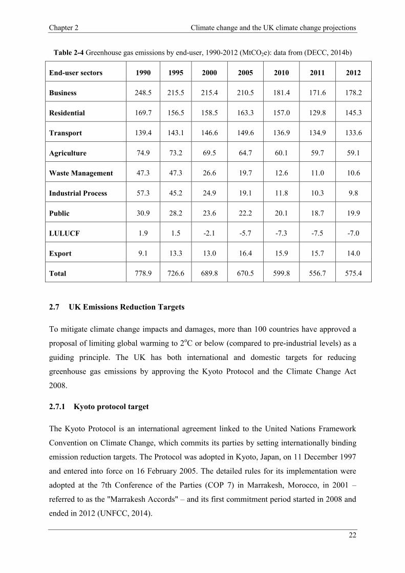
Chapter 2 Climate change and the UK climate change projections
22
Table 2-4 Greenhouse gas emissions by end-user, 1990-2012 (MtCO2e): data from (DECC, 2014b)
End-user sectors 1990 1995 2000 2005 2010 2011 2012
Business 248.5 215.5 215.4 210.5 181.4 171.6 178.2
Residential 169.7 156.5 158.5 163.3 157.0 129.8 145.3
Transport 139.4 143.1 146.6 149.6 136.9 134.9 133.6
Agriculture 74.9 73.2 69.5 64.7 60.1 59.7 59.1
Waste Management 47.3 47.3 26.6 19.7 12.6 11.0 10.6
Industrial Process 57.3 45.2 24.9 19.1 11.8 10.3 9.8
Public 30.9 28.2 23.6 22.2 20.1 18.7 19.9
LULUCF 1.9 1.5 -2.1 -5.7 -7.3 -7.5 -7.0
Export 9.1 13.3 13.0 16.4 15.9 15.7 14.0
Total 778.9 726.6 689.8 670.5 599.8 556.7 575.4
2.7 UK Emissions Reduction Targets
To mitigate climate change impacts and damages, more than 100 countries have approved a
proposal of limiting global warming to 2oC or below (compared to pre-industrial levels) as a
guiding principle. The UK has both international and domestic targets for reducing
greenhouse gas emissions by approving the Kyoto Protocol and the Climate Change Act
2008.
2.7.1 Kyoto protocol target
The Kyoto Protocol is an international agreement linked to the United Nations Framework
Convention on Climate Change, which commits its parties by setting internationally binding
emission reduction targets. The Protocol was adopted in Kyoto, Japan, on 11 December 1997
and entered into force on 16 February 2005. The detailed rules for its implementation were
adopted at the 7th Conference of the Parties (COP 7) in Marrakesh, Morocco, in 2001 ‒
referred to as the "Marrakesh Accords" ‒ and its first commitment period started in 2008 and
ended in 2012 (UNFCC, 2014).

Chapter 2 Climate change and the UK climate change projections
23
2.7.1.1 The target
On 31 May 2002 the UK ratified the Kyoto Protocol, along with fifteen other European
Union (EU) member states. The EU has a joint target to reduce its emissions by 8%
compared with the base year level (1990) over the first commitment period (2008-2012). The
Protocol uses 1990 as a base year for CO2 reduction and, within this arrangement, the UK
agreed to reduce its GHG emissions by an average of 12.5% below base year levels over the
five year period of 2009 to 2012 (DECC, 2014b).
In July 2007, the UK base year estimation of the Kyoto basket of GHGs was set at 779.9
million tons of CO2 equivalent (MtCO2e). In accordance with this estimate, to meet the Kyoto
commitment, the UK’s GHG emissions need to be below 682.4 MtCO2e on average per year
during the period of 2008-2012 (DECC, 2014a).
2.7.1.2 Performance
Table 2-5 compares UK’s progress towards meeting the Kyoto Protocol target with an
assigned carbon budget over the first commitment period of 2008-2012. Together with
emissions trading, provisional estimates for 2012 show the emissions to be 585.4 MtCO2e,
which is 24.9% below the baseline (DECC, 2014b).
For the second Kyoto Protocol commitment period, which will run for eight years from 2013
to 2020 inclusive, the EU has made a commitment, largely consistent with its own target, to
reduce emissions by an average of 20% below base year levels.
Table 2-5 Kyoto Protocol: data from (DECC, 2014a)
Assigned amount
(MtCO2e)
Actual emissions including EU Emissions Trading System
(EU ETS) (MtCO2e)
Overall
emissions
below
assigned
amount
2008-12
(MtCO2e)
Total
emissions
(2008-12)
Equivalent
average
emissions
(p.a.)
2008 2009 2010 2011
2012
Cumulative
emissions
(2008-12)
3412 682 610 590 601 577 585 2962 450

Chapter 2 Climate change and the UK climate change projections
24
2.7.2 The Climate Change Act 2008
The Climate Change Act 2008 also provides an interim target and obligatory framework to
reduce GHG emissions; consequently, the UK is committed to reduce emissions by at least
80% by 2050, compared to 1990 baselines. To meet this target by 2020 the UK must cut its
GHG emissions by at least 34% compared to the 1990 baseline (DECC, 2014a).
2.7.2.1 The target
The UK Government set the following four carbon budgets covering the periods 2008-12,
2013-17, 2018-2022 and 2023-27:
1. Total GHG emissions will not exceed 3,018 million tonnes CO2 equivalent over the
five-year period 2008-12, which is 22% below the base year level on average over the
period.
2. Total GHG emissions set to 2,782 MtCO2e of over the five-year period 2013-17,
which equates to 28% below the base year level on average over the period.
3. Total GHG emissions should not exceed 2,544 MtCO2e over the five-year period
2018-22, which is about 34% below the base year level.
4. A reduction in emissions of 50% below base year levels over the period 2023-2027
(DECC, 2014a).
2.7.2.2 Performance
Excluding emissions trading in 2012, emissions on a carbon budgets basis were provisionally
estimated to be 568.2 MtCO2e, which is 26.6% below the baseline. Including emissions
trading, accounting for the effect of emissions trading increases the UK’s emissions in 2012
on a carbon budgets basis to 581.8 MtCO2e, which is 24.9% below the baseline.
This reduction has been achieved through regulations, legislations and programme aimed at
cutting the anthropogenic sources of GHGs. In addition, climate change projections and
scenarios have enhanced the potential for intervention in order to reduce expected climatic
stimuli or their effects. Table 2-6 summarizes these results alongside equivalent figures for
2011 (DECC, 2014a).

Chapter 2 Climate change and the UK climate change projections
25
Table 2-6 The Climate Change Act 2008: data from (DECC, 2014a)
carbon budget(MtCO2e) Budget 1 Budget 2 Budget 3 Budget 4
2008-12 2013-17 2018-22 2023-27
Budget level 3,018 2,782 2,544 1,950
Equivalent average annual emissions(p.a.) 603.6 556.4 508.8 390
2.8 Climate Change Mitigation Potential of Building in Near and Long Term
As mentioned in Sections 2.5 and 2.6, in developed countries, such as the UK, the residential
sector is the second contributor and responsible for 25% of global GHG emissions, therefore
buildings are their principal contributors; hence they have an important effect on global
warming, while, at the same time, their performance depends on the climate to which they are
exposed. It is important, at an early design stage, to assess and model buildings’
performances, which includes their propensity to mitigate future climate changes. Therefore,
sets of current and future weather data are required in order to appropriately assess the
environments and conditions likely to be experienced at their proposed locations. Such data
need to be derived from weather observations stretching back over a period of between 20-30
years (Levermore, et al., 2012).
2.9 Current UK Hourly Weather Data
2.9.1 CIBSE hourly weather data
Since the early 1980s, the UK’s Charted Institution of Building Services Engineers (CIBSE)
has recognised the term “Reference Weather Years (RWYs)”, which represents an average
year for a given location and time frame (CIBSE, 2002). The “RWY”, therefore, is a year, or an
average of years, that represents the range of weather patterns typically found in a multi-year dataset
(Hacker, et al., 2009; Holum and Hitchin, 1978).
Example Weather Years (EWYs) were the first basis for a UK RWY and also the first set of
weather years developed by CIBSE. EWYs were real historical years having monthly
conditions very similar to the average values for sets of many years of data. Obviously, there
was only a very small chance of finding a truly representative year in which all months are
typical (Hacker, et al., 2009). For that reason, improved weather year data sets were launched
by CIBSE in the 1990s and this led to the development of new “typical years” and “near
extreme warm summer years”. The CIBSE (2002) called these the “Test Reference Years”
Chapter 2 Climate change and the UK climate change projections
26
(TRY) and the “Design Summer Years” (DSY). TRY files are used to define the average
annual energy consumption and DSY files are intended primarily to evaluate the risk of
summer overheating. However, both TRYs and DSYs were originally only available for three
locations ‒ London, Manchester and Edinburgh ‒ but, since 2005, greater geographical
coverage has been obtained from further locations and current CIBSE TRY and DSY hourly
weather data set are available for fourteen sites (CIBSE, 2002).
As a consequence of these changes, instead of one typical year, the TRY consists of twelve
separate typical months of data, not necessarily from the same year. Three weather variables
‒ dry bulb temperature, wind speed and global horizontal solar irradiation ‒ from twenty-
three years of data, from 1983 to 2005, were compared to select these typical months using
Finkelstein-Schafer (F-S) statistics (Finkelstein and Schafer, 1971; Hacker, et al., 2009).
2.10 Future Hourly Weather Data
It is essential to obtain currently available weather files in order to evaluate, and mitigate the
causes of, climate change origin from buildings’ design. There is also a need to consider the
potential effects of future climate change at an early stage in the design process; therefore, to
be able to increase a building’s adaptive capacity, designers need future projected weather
files so they can model, predict and assess its likely performance. Such data can now be
generated from various climate change scenarios.
There are, however, significant uncertainties regarding risks that buildings may face due to
possible changes of climate; therefore, different models and story lines depicting future GHG
emissions need to be developed to enable designers to carry out both qualitative and
quantitative impact assessments in order for them to appraise the merits of alternative
conversion options.
2.10.1 General circulation models
General circulation models (GCMs), which simulate past natural and physical changes in
oceanic, atmospheric and other environmental circulation patterns, illustrate how these
processes may affect climate systems and how they may predict the possible trajectory of
climate change. Also, the creation of complete global climate models, known as ‘atmosphere-
ocean global circulation models’ (AOGCMs) and the range of their processes has been
developed over time by the IPCC (Hacker, et al., 2009; Bernstein, et al., 2007).

Chapter 2 Climate change and the UK climate change projections
27
2.10.2 Emission Scenarios
In order to incorporate the widest possible range of patterns of GHG emissions into climate
change scenarios, it was necessary to create emissions scenarios and the IPCC Special Report
on Emissions Scenarios (SRES), which is based on likely further economic trends, is the one
chosen to demonstrate UK regional climate projections. Six storylines, ranging from low to
high emissions, are assumed by the IPCC in relation to future population, economic and
industrial developments. For the lowest emission scenario, where sustainability is the
dominant driver, atmospheric CO2 is predicted to be 549 Parts per Million (PPM); whereas,
for the highest emission scenario, in which economic growth is the main driver, atmospheric
CO2 of 970 PPM is predicted (Nakicenovic, 2000). Figure 2-11 compares three different
emission scenarios in climate projection.
Figure 2-11 The IPCC low (B1), medium (A1B) and high (A1FI) emissions scenarios as used in the
UKCP09 climate projections (Costello and Mylona, 2014)
2.10.3 UKCIP and UKCP
In 1997, in order to project GCMs and emission scenarios that would enable regional climate
change projections to be generated, the government established the UK Climate Impacts
Programme (UKCIP) by which practice-based research provides help and advice for building
organisations and stockholders to adapt to changing climate conditions (UKCIP, 2014;
Willows and Connell, 2003). The first set of projections, UKCIP98, which were produced by
using coupled AOGCMs, had a spatial resolution of approximately 350 km. These led to new

Chapter 2 Climate change and the UK climate change projections
28
sets of projections – by UK Climate Change Projection (UKCP) – that resulted in more
sophisticated climate models with improved spatial resolutions, UKCP09 scenarios. (Hacker,
et al., 2009). Since the probability of different amounts of change indicates the strength of
evidence relating to expected changes in climate, the progression from UKCIP02 to UKCP09
denoted a move towards the creation of more probabilistic frameworks, more transparent
demonstrations and more detailed quantitative assessments of uncertainty. Table 2-7
demonstrates the changes from UKCIP02 to UKCP09, compares and clarifies the time slices
used for calculation and projection.
The probabilities used in UKCP09 are Cumulative Distribution Function (CDF) probabilities
in the range 0-100%. Thus, in this case, they give the likelihood of climate change being less
than a given value. For instance, a 90 percentile change in temperature means it is ‘very
likely’, or there is a 90% chance, of actual climate change values being lower than that value,
while a 10 percentile of change in temperature means that it is ‘very unlikely’, or there is a
10% chance, of the actual climate change being lower than that value. The climate change at
50% probability level is that which is ‘likely’ as not being exceeded and is called ‘central
estimate’ (UKCP, 2011).
Table 2-7 Time periods used in UKCP09 and UKCIP02: data from (UKCP, 2011)
UK climate
projections Baseline 2020s 2030s 2040s 2050s 2060s 2070s 2080s
UKCIP02 1961 to
1990
2011 to
2040 _ _
2041 to
2070 _ _
2071 to
2100
UKCP09 1961 to
1990
2010 to
2039
2020 to
2049
2030 to
2059
2040 to
2069
2050 to
2079
2060 to
2089
2070 to
2099
2.10.4 Generation of weather years
These UKCIP climate projections are difficult for building designers to use as the changes in
climate variables are expressed over average annual, seasonal or monthly periods, whereas, in
most cases, designers require building thermal simulation models to be based on daily, or
sub-daily, intervals in order to assess a building’s likely performance. There are, therefore,
different methods for generating the future “hourly weather files” from UKCIP projections,
such as dynamic downscaling, analogue scenarios, morphing (time series adjustment) and

Chapter 2 Climate change and the UK climate change projections
29
weather generators (stochastic models). For instance, Exeter University, using the
‘PROMETHEUS methodology’, has published Energy Plus weather (EPW) files for forty-
five locations across the UK. These files are created using the UKCP09 weather generator
(University of Exeter, 2012; University of Exeter, 2011). More details on EPW files can be
seen in Chapter 5.
Figure 2-12 compares mean monthly dry-bulb temperatures, for Heathrow by Exeter
University, for different probabilities by using generated future weather files ‒ 2050-High
emission scenario .The figure indicates that, (i) for all percentiles the changes are generally
larger in summer, (ii) for maximum temperature, the changes in summer are around twice
those for winter, (iii) the summer increases are considerably larger than the annual mean
change, (iv) the change in minimum temperature is less than for maximum temperature, and
(v) there is an increase in diurnal temperature range.
A group at Manchester University, working on the Co-incident Probabilistic climate change
weather data for a Sustainable Environment (COPSE) project, has also used UKCP09
weather generator to produce TRY and Design Reference Year (DRY) files for any location
covered by UKCP09 (Watkins, et al., 2011).
CIBSE Future weather Years in TRY and DSY format are generated based on ‘morphing
methodology’. Figure 2-13 compares mean dry-bulb temperatures for different emission
scenarios and time-scales generated by CIBSE using UKCIP02. It can be seen from the figure
that, from the middle of the century onwards, the differences in emission scenarios take effect
and the high emissions scenario from the low scenario. UKCIP02 projections in global mean
annual near-surface air temperature show that, by the 2080s, the global average temperature
is predicted to have increased by between 2.0°C and 3.9°C since the 1970s.

Chapter 2 Climate change and the UK climate change projections
30
Figure 2-12 Comparison of average monthly dry-bulb temperatures of ‘Heathrow-2050-High
emission scenario’ for different probabilities: data from (Eames, et al., 2010; University of Exeter,
2012)
Figure 2-13 Comparison of average outside dry bulb temperature of various emission scenarios and
time scales in UKCIP02. Current and future Heathrow CIBSE TRY weather files: data from (Eames,
et al., 2010; University of Exeter, 2012)
0
5
10
15
20
25
30
Jan Feb Mar Apr May Jun Jul Aug Sep Oct Nov Dec
Current 2050-Low 2050-High 2080-Low 2080-High

Chapter 2 Climate change and the UK climate change projections
31
2.11 Summary and Conclusion
There is now widespread scientific agreement that human activity has been the predominant
stimulus for climate change, which is perhaps the greatest pressing environmental, social and
economic issue facing the planet today. Various policies, agreements and actions, both
globally and within the UK, have been introduced aimed at minimising its causes and at
adapting to its inevitable impacts precipitately and sustainably. An important step towards
these goals is to create methods of exploring in what ways human activities have contributed
to the various climate change scenarios that are currently underway.
It has been clearly established that energy use in buildings, including residential buildings, is
a principal source of GHG emissions that contribute to climate change, which, in turn, will
have a significant impact on the built environment by affecting summertime thermal comfort
alongside the amount of energy required to heat and cool buildings. Consequently, in order to
project regional future climate change and emission scenarios the government established the
UK Climate Impacts Programme (UKCIP) by which practice-based research provides help
and advice for building organisations and stockholders to adapt to changing climate
conditions. Therefore, it is important to tackle climate changes by utilizing UKCIP scenarios,
for predicting energy performance of both new and existing buildings, which would lead to,
(i) significant reductions in CO2 emissions, (ii) improvements in occupants’ comfort levels,
(iii) reductions in operating costs, and (iv) improvements in their sustainability and resilience.
However, discrepancies between different climate scenarios and some real-time monitoring
results, suggest that these should not be regarded as “forecasts of future climate”, but as
“internally-consistent pictures of possible future climates”, each reliant on an assortments of
prior assumptions.
The UK’s estimated GHG emissions for 2011 indicated that 24% of GHG emissions by the
end-user sector were generated by the residential sector. Thus, the next chapter will discuss
current UK housing stock, carbon emission reduction regulations, programs and actions
together with climate change mitigation potentials of existing housing stock.

Chapter 3 – Eco-Refurbishment of Existing UK Housing
Stock
3 not erase
not erase this
not erase
Chapter 3 Eco-refurbishment of existing UK housing stock
32
3.1 Chapter Overview
In 2013 UK dwellings produced 77MtCO2 emissions of CO2– an increase of 3% from 2012.
These emissions represented approximately 17% of all UK emissions and 25% of UK GHG
end-user emissions, thus contributing to potential changes in the climate, some of which
might adversely affected buildings (DECC, 2014b). Since about 70% of all UK homes will
still be in use by 2050, low-carbon refurbishment is critical if the national 80% carbon
reduction goal is to be met. However, climate change is not the only reason for improving the
energy performance of existing homes. Energy inefficiency, which is a significant driver of a
household’s potential fuel poverty, is another reason for improvement. Even though energy
efficiency schemes have meant that fuel poverty in the UK had, by 2013, fallen by 18% from
its 2009 total, 4.5 million households were still unable to heat their homes properly (DECC,
2014c). The conclusion, therefore, must be that houses have to perform better in terms of
energy. Hence, this chapter will focus on the challenges of improving energy performance of
existing UK housing stock by, (i) analysing the UK housing stock, (ii) examining energy
efficiency initiatives and regulations, and (iii) analysing related case studies from one of the
largest housing carbon reduction schemes – ‘Retrofit for the Future’.
3.2 UK Housing Stock
3.2.1 Age, energy trends and energy efficiency of stock
The UK’s 22.7 million homes account for over a quarter of its current CO2 emissions, most of
which is expended on space and water heating. According to the Housing Energy Fact File, in
2013, 62% of the energy in an average house was used for heating, 18% for hot water, 17%
for lighting and electrical appliances and less than 3% for cooking – see Figure 3-1 (Palmer
and Cooper, 2014). Therefore, the two main energy efficiency goals for existing dwellings
are, (i) improving their electrical and gas services, and (ii) upgrading their building fabric in
order to reduce heat loss. According to the latest English Housing Survey (2012), of the
estimated 22.7 million English dwellings, 70% of them – i.e. more than 17.5 million – were
built before 1976, when insulation became a legal Building Regulations requirement. Of
these 17.5 million, 80% are considered to be ‘inefficient’ houses. Overall, the UK is
considered to have the oldest and least efficient residential sector in the developed world.
Figure 3-2 illustrates the percentage of houses with insulation. Among 18.1 million houses in

Chapter 3 Eco-refurbishment of existing UK housing stock
33
the UK only 7.6 million of them have wall insulation which are mostly houses with cavity
wall (DCLG, 2014).
Figure 3-1 UK housing stock and climate change: data from: (Palmer and Cooper, 2014)
Figure 3-2 Number of dwellings with insulation in 2012: data from: (DCLG, 2014)
0
10
20
30
40
50
60
70
80
90
Terrace Semi-detached Detached Bungalow
%
Wall insulation Loft insulation Double glazed windows

Chapter 3 Eco-refurbishment of existing UK housing stock
34
3.2.2 Decent, non-decent and hard to treat houses
If a house meets all four principles, listed below, it is called ‘decent’ – if it does not then it is
termed ‘non-decent’.
1. It must meet the current statutory minimum standard for housing as set out in the
Housing Health and Safety Rating System (HHSRS).
2. It must be in a reasonable state of repair, related to the age and condition of a range of
building components, including walls, roofs, windows, doors, chimneys, electrics and
heating systems.
3. It must have reasonably modern facilities and services in terms of the age, size and
layout/location of the kitchen, bathroom, toilets and its level of noise insulation; this
includes ‘common areas’ in blocks of flats.
4. It must provide a reasonable degree of thermal comfort in regard to insulation and
heating efficiency (DCLG, 2006).
The term ‘non-decent home’ is often referred to as a ‘hard-to-treat’ home (HTT), the majority
being solid-walled houses that would not benefit from relatively simple energy-efficiency
interventions. In a 2008 Building Research Establishment (BRE) report, four classifications
of dwellings were considered to be HTTs, (i) solid walled, (ii) off the gas network, (iii)
without a loft, and (iv) high rise flats. Figure 3-3 depicts the relationship of each category and
percentage of dwellings in each category (BRE Housing, 2008).
Figure 3-3 Showing the relationship between the HTT categories with the percentage of the HTT
stock (BRE Housing, 2008)

Chapter 3 Eco-refurbishment of existing UK housing stock
35
In 2012, 4.9 million dwellings failed to meet the ‘decent’ homes criteria, down 6% from the
22% recorded in 2006 (DCLG, 2011) . Figure 3-4 compares the number of non-decent houses
together with their ages and types. The figure shows clearly that solid walled terraced houses
make up the largest proportion of HTT houses.
Figure 3-4 Non decent dwellings by dwelling age band and type: data from (DCLG, 2014)
3.3 Refurbishment vs. New Build
In spite of all the energy efficiency challenges relating to the existing housing stock, there are
very good reasons for considering refurbishment rather than new-build. Because of dwindling
resources, sustainability should be considered in its broadest sense when reducing carbon
emissions. The UK’s housing stock has evolved over generations and its houses represent not
only an early example of mass urban living but also a strong cultural and architectural
heritage. Consequently, when improving dwelling energy efficiency, great care must be taken
not to disfigure or destroy their aesthetic and historic value, since that would have a social
and visual impact on communities and the environment (Power, 2008). Likewise, BRE’s
2009 publication, ‘Knock It Down or Do It Up’, highlights the significance of excessive
GHG emissions due to the inevitable waste generated from traditional construction and
demolition methods. The publication also set off the arguments of English Heritage and
-
200
400
600
800
1,000
1,200
1,400
pre 1919 1919-1944 1945-1964 1965-1980 post 1980
Num
ber
of
ho
use
s (0
00
s)
terraced house semi-detached house bungalow or detached house flat

Chapter 3 Eco-refurbishment of existing UK housing stock
36
Commission for Architecture and the Built Environment (CABE), who advocate the
importance of old buildings in place making (Plimmer, et al., 2008)
Although achieving the required carbon savings by refurbishment as compared to new build
has been questioned in some quarters, the replacement rate of old houses is approximately
1.0% to 3.0% per annum. This means that some 70% of all current UK houses will still exist
into the 2050s; therefore, low carbon refurbishment is critical if the CO2 reduction goal of
80% is to be met (Boardman, al, et, 2005; Lowe, 2007).
In its first report to government, the Committee on Climate Change (CCC), set up in 2008 in
conjunction with the Climate Change Act, stated firmly that sustainable refurbishment of
existing buildings must take place on a much larger scale. The CCC estimated that the
cumulative reduction in GHG emissions from existing buildings far surpasses those of new
buildings (CCC, 2011).
3.4 Sustainable, Green or Eco-Refurbishment
Sustainable, green or eco-refurbishment, in the context of carbon reduction, is all about
making buildings more thermally efficient and sustainable. The emphasis, therefore, should
be on demand reduction rather than on the energy supply. Therefore, in terms of reaching
eco-refurbishment standards, five areas of eco-refurbishment should be focused on: (i) using
fuels that have low carbon intensity, (ii) improving building envelope air-tightness, (iii)
reducing building envelope heat bridges, (iv) using integrated building renewables, and (v)
the possible use of solar energy. Essentially, this suggests that a typical eco-refurbished house
should be super-insulated with triple-glazed windows and be fitted with a mechanical
ventilation and heat recovery system (MVHR), which has a small heating element within its
ventilation system in order to improve the internal air quality (Urban grown, 2009).
3.5 An Overview of the Regulations and Government Schemes on Refurbishment
It is estimated that, in order to meet the 2050 carbon reduction target, 5,000 houses will need
to be refurbished every day. To date, though, the rate of refurbishment is much slower.
However, the UK government has shown an understanding of the crucial roles that
refurbishment and retrofits must play in meeting the carbon reduction goal, and have
launched initiatives to stimulate the rate of refurbishment. Some of these initiatives include

Chapter 3 Eco-refurbishment of existing UK housing stock
37
the Green Deal Finance Package, Feed-in Tariffs, and the Renewable Heat Incentive. In the
following sections the most common regulations and schemes will be described.
3.5.1 Standard Assessment Procedure (SAP)
The Standard Assessment Procedure (SAP) has, since 1993, been an integrated, independent
methodology used for evaluating and certifying dwelling performance against Building
Regulations. It is at the core of the UK Government’s policy for identifying and assessing the
energy upgrading needs of the UK’s existing dwellings (Part L1B) and for meeting the
energy requirements of newly constructed dwellings (Part L1A). SAP, which uses a scale
from 1, the least efficient house, to 100, the most efficient, calculates energy performance
with a view to awarding certificates (Energy Performance Certificates, EPCs – see 3.5.3
below) following the 2002 introduction of energy rating requirements under the EU’s Energy
Performance of Buildings Directive (EPBD) (Killip, 2011). Figure 3-5 illustrates how SAP
ratings relate to EPC ratings. However, with actual energy performance results now available,
large discrepancies have been found between measured energy performance and the SAP
predicted performances. This will be discussed further in Chapter 5.
Figure 3-5 illustrates how SAP rating relates to EPCs (BRE, 2012c).

Chapter 3 Eco-refurbishment of existing UK housing stock
38
3.5.2 Building Regulations Part L (England and Wales)
Building Regulation Part L1B constitutes the minimum standards that any existing property
requires in order to meet fuel and power conservation targets in England. However, the
minimum criteria differ across the UK; the best practice recommendation for England is for
an air permeability reading of 5m3/(h.m
2)@50Pa (EST, 2007). English standards for existing
buildings fabric are summarised in Table 3-1. For new build properties, a zero carbon target
was set for dwellings from 2016, which, under the 2006 regulations, requires a 25% reduction
in CO2 emissions, rising to 44% reduction in 2013 (BRE and EST, 2012).
Table 3-1 Best practice recommended improvements (BRE, 2011)
Measures Required U-Value after improvement (W/m2K)
Walls 0.30
Roofs 0.16
Flat roofs 0.25
Exposed Floors 0.20-0.25 (depending upon floor geometry)
Solid doors 1.00
Half glazed doors 1.50
3.5.3 Energy Performance Certificate (EPC)
In 2002 the European Union’s Energy Performance of Buildings Directive 2002/91/EC
(European Commission 2002), which applies to all buildings, was introduced. It required
each member state to establish an energy rating method and labelling system for houses. This,
in the UK, is recognised by the award of an Energy Performance Certificate (EPC) if a house
meets a set of criteria based on a theoretical model of the potential performance of its design
fabric. This model places a house on a scale from the least to the most energy-efficiency
rating (A to G) based on standardised information about current and potential running costs
and on the provision of advice regarding energy efficiency and low-carbon improvements.

Chapter 3 Eco-refurbishment of existing UK housing stock
39
EPCs, together with property particulars, are valid for ten years (BRE and EST, 2012).
Reduced-data versions of the SAP (RdSAP) methodology are used to produce EPCs by
qualified domestic energy assessors (BRE, 2011).
3.5.4 Passivhaus and EnerPHit standard
Among the various different building codes, regulations and standards that have been
developed to mitigate climate change and global warming; the Passivhaus certification
applies the strictest criteria regarding heating demand. The Passive House Planning Package
(PHPP) is used to estimate a building’s airtightness, heating, cooling and primary energy
demand, including an amount that takes into account overheating during colder periods. The
package, which is also used when planning a Passive House, serves as a basis of verification
and certification for meeting the Passive House Standard (Passive House Institute, 2012). The
EnerPHit Standard (Quality-Approved Modernisation with Passive House Components),
which has recently been developed as a good practice refurbishment guide for Passivhaus
renovations, sets a slightly lower than the full Passivhaus standard requirement for new build;
an old building can also receive such a certificate (see Table 3-2).
Table 3-2 The Passivhaus and EnerPHit energy standards as applied to a typical dwelling (AECB
CarbonLite Programme, 2007)
Standard Space heating
(kWh/m2/yr)
Primary Energy
Consumption
(kWh/m2/yr)
CO2 Emission
(kg/m2/yr)
Pressurisation
test
(hr @ 50Pa)
EnerPHit 25 120 No explicit limit <1.0
PassivHaus 15 120 No explicit limit <0.6
PassivHaus in the
UK context 15 78 15 <0.6

Chapter 3 Eco-refurbishment of existing UK housing stock
40
3.5.5 Retrofit for the future programme
To encourage companies to deal with climate change and other renovation challenges, in
March 2009 the UK’s Technology Strategy Board (TSB) launched an initiative called
‘Retrofit for the Future’‒ a competition leading to the funding of a £17m refurbishment
scheme initiative aimed at meeting targets in carbon reduction emissions and energy use
(EST, 2009a). The TSB ‘Retrofit for the Future’ competition encouraged collaboration
between housing providers, designers, contractors and researchers in order to inspire them to
grasp new business opportunities in the retrofit market. The scheme involved two phases ‒
Phase 1 examined the 194 design and feasibility studies submitted, of which 86 were
accepted and moved into Phase 2, where the applicants were offered 100% implementation
funding. The key focus was on developing ambitious and cost-effective methods of achieving
deep cuts in CO₂ emissions. The programme was looking for innovative plans with
prospective widespread applicability in low rise, whole house retrofitting (TSB, 2013; LEB,
2009).
3.5.5.1 Retrofit for the future energy performance target
the purpose of this competition, energy performance targets, which were developed by the
Association for Environment Conscious Building (AECB), were linked to the Climate
Change Act 2008, which sought an 80% reduction in CO2 emissions, compared to 1990
levels. A suitable proxy target was identified by estimating the performance of a typical 1990,
80m² three-bedroom semi-detached property (LEB, 2009). An estimated primary energy
demand of 365 kWh/m2/year and emission rate of 104kgCO2/m
2/year was required for a
typical house in terms of the scheme (Oxford Brookes University, 2011). From this figure, an
80% reduction resulted in a primary energy target of 115kWh/m2/year and a CO2 emissions
target of 17kgCO2/m2/year (LEB, 2009). However, some of the projects submitted achieved
higher savings and received other AECB certificates. The standards applied were either
expressed in terms of a combination of limits on space heating energy and primary energy
consumption and CO2 emissions (see Table 3-3), or as a percentage saving in energy and CO2
emissions relative to the same building type in the existing building stock which is quoted in
Table 3-4 (AECB CarbonLite Programme, 2007).

Chapter 3 Eco-refurbishment of existing UK housing stock
41
Table 3-3 The three energy standards as applied to a typical dwelling (AECB, 2007)
Standard Space heating
(kWh/m2/yr)
Primary
Energy
Consumption
(kWh/m2/yr)
CO2 Emission
(kg/m2/yr)
Pressurisation
test
(hr @ 50Pa)
Silver 40 120 22 No explicit
limit
EnerPHit 25 120 No explicit
limit <1.0
PassivHaus 15 120 No explicit
limit <0.6
PassivHaus in the
UK context 15 78 15 <0.6
Gold 15 58 4 No explicit
limit
Table 3-4 Percentage reduction in CO2 emissions relative to the building stock (AECB, 2007)
Standard
Reduction in primary energy
consumption compared to average
UK building of that type
Reduction in CO2 emissions
compared to average UK building
of that type
Silver 70% 70%
PassivHaus 80% 80%
Gold 85% 95%
3.5.6 Analysis of the monitoring data of competition entries
The monitoring data of all 86 ‘Retrofit for the Future’ projects have now been published at
the Retrofit Analysis website. Analysis of the data from 37 of those properties found that
three projects achieved the desired 80% reduction in CO2 emissions, with 23 reaching
between 50% and 80%. Among these projects, the new build ‘Camden House’ in London was
certified to Passivhaus standard. Together with the retrofitted projects, the ‘Oxford Whole
House Carbon Reduction Project’ and the ‘100 Princedale Road Passivhaus project in
London’ were certified to EnerPHit standard by significantly improving energy performance
and achieving deep cuts in CO₂ emissions. The energy performance analysis of these cases is
presented in this section (TSB, 2013).
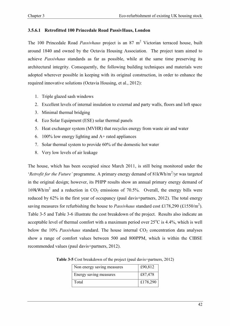
Chapter 3 Eco-refurbishment of existing UK housing stock
42
3.5.6.1 Retrofitted 100 Princedale Road PassivHaus, London
The 100 Princedale Road Passivhaus project is an 87 m2 Victorian terraced house, built
around 1840 and owned by the Octavia Housing Association. The project team aimed to
achieve Passivhaus standards as far as possible, while at the same time preserving its
architectural integrity. Consequently, the following building techniques and materials were
adopted wherever possible in keeping with its original construction, in order to enhance the
required innovative solutions (Octavia Housing, et al., 2012):
1. Triple glazed sash windows
2. Excellent levels of internal insulation to external and party walls, floors and loft space
3. Minimal thermal bridging
4. Eco Solar Equipment (ESE) solar thermal panels
5. Heat exchanger system (MVHR) that recycles energy from waste air and water
6. 100% low energy lighting and A+ rated appliances
7. Solar thermal system to provide 60% of the domestic hot water
8. Very low levels of air leakage
The house, which has been occupied since March 2011, is still being monitored under the
‘Retrofit for the Future’ programme. A primary energy demand of 81kWh/m2/yr was targeted
in the original design; however, its PHPP results show an annual primary energy demand of
169kWh/m2 and a reduction in CO2 emissions of 70.5%. Overall, the energy bills were
reduced by 62% in the first year of occupancy (paul davis+partners, 2012). The total energy
saving measures for refurbishing the house to Passivhaus standard cost £178,290 (£1550/m2).
Table 3-5 and Table 3-6 illustrate the cost breakdown of the project. Results also indicate an
acceptable level of thermal comfort with a maximum period over 25oC is 4.4%, which is well
below the 10% Passivhaus standard. The house internal CO2 concentration data analyses
show a range of comfort values between 500 and 800PPM, which is within the CIBSE
recommended values (paul davis+partners, 2012).
Table 3-5 Cost breakdown of the project (paul davis+partners, 2012)
Non energy saving measures £90,812
Energy saving measures £87,478
Total £178,290
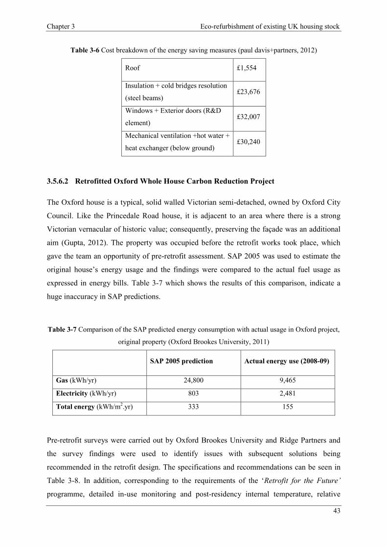
Chapter 3 Eco-refurbishment of existing UK housing stock
43
Table 3-6 Cost breakdown of the energy saving measures (paul davis+partners, 2012)
Roof £1,554
Insulation + cold bridges resolution
(steel beams) £23,676
Windows + Exterior doors (R&D
element) £32,007
Mechanical ventilation +hot water +
heat exchanger (below ground) £30,240
3.5.6.2 Retrofitted Oxford Whole House Carbon Reduction Project
The Oxford house is a typical, solid walled Victorian semi-detached, owned by Oxford City
Council. Like the Princedale Road house, it is adjacent to an area where there is a strong
Victorian vernacular of historic value; consequently, preserving the façade was an additional
aim (Gupta, 2012). The property was occupied before the retrofit works took place, which
gave the team an opportunity of pre-retrofit assessment. SAP 2005 was used to estimate the
original house’s energy usage and the findings were compared to the actual fuel usage as
expressed in energy bills. Table 3-7 which shows the results of this comparison, indicate a
huge inaccuracy in SAP predictions.
Table 3-7 Comparison of the SAP predicted energy consumption with actual usage in Oxford project,
original property (Oxford Brookes University, 2011)
SAP 2005 prediction Actual energy use (2008-09)
Gas (kWh/yr) 24,800 9,465
Electricity (kWh/yr) 803 2,481
Total energy (kWh/m2.yr) 333 155
Pre-retrofit surveys were carried out by Oxford Brookes University and Ridge Partners and
the survey findings were used to identify issues with subsequent solutions being
recommended in the retrofit design. The specifications and recommendations can be seen in
Table 3-8. In addition, corresponding to the requirements of the ‘Retrofit for the Future’
programme, detailed in-use monitoring and post-residency internal temperature, relative

Chapter 3 Eco-refurbishment of existing UK housing stock
44
humidity and internal CO2 levels evaluations were undertaken over a two years period
(January 2011 to January 2013). Initial results show an 80% reduction in CO2 emissions and
a 58.6% reduction in total energy consumption (Gupta, 2012).
Table 3-8 Specification and recommendations in retrofit design of the house (Oxford Brookes
University, 2011)
Key findings Low carbon refurbishment proposals
Poor daylight levels in most rooms Sun-pipe with good U-values
Poor indoor air quality throughout MVHR for good air quality; optimise airtightness
Un-insulated fabric; difficult to heat house for
comfort Highly insulated fabric, triple glazing, MVHR
Future adaptability for residents change to with
health issues
Potential for living room change to Bedroom and
refurbishment of ground floor toilet to a wet
room
3.5.6.3 New build Camden PassivHaus
The Camden new-built Passivhaus project is a 101 m2, two story detached house in Camden,
North London, designed by Bere Architects. Like other Passivhaus designs it has MVHR
system, high levels of insulation and air-tightness using a prefabricated timber frame and
triple glazed windows. SAP 2005 and PHPP were used to estimate and predict energy
performance (Palmer, 2011). It is also being monitored under the TSB Building Performance
Evaluation scheme. A summary and comparison of SAP, the Passivhaus Planning Package
(PHPP) estimates and real performances are shown in Table 3-9.
It is worth to analyse and compare the performance of this new build house with the
refurbished ones as the house is one of the lowest energy dwellings ever monitored in the
UK, with the annual space heating demand of 12.1kWh /m2 easily meeting the 15 kWh/m
2
Passivhaus target and the annual energy demand of 125kWh/m2
slightly surpassing the 120
kWh/m2/yr target.
The degree of internal comfort shows very good indoor air quality, internal temperature,
internal CO2 concentration and ventilation rate. However, when the occupants were asked
about summertime thermal comfort they stated that “when it got hot, it got very hot” although

Chapter 3 Eco-refurbishment of existing UK housing stock
45
they resolved this by opening windows. However, they reported that they enjoyed the warm
summer temperatures, so they didn’t regard overheating to be a problem (Ridley, et al.,
2013).
Table 3-9 Camden Passivhaus measured and monitored energy consumption (Palmer and Cooper,
2014)
SAP PHPP Monitoring
Space Heating (kWh/yr) 1572 1348 1420
Water Heating (kWh/yr) 3708 2218 1570
Lighting (kWh/yr) 1464 1822 623
3.6 Learning Points from the Case Studies
Of the projects presented, the first two were in the conservation area and revealed a huge
number of challenges at different stages of planning and construction. Examining these
challenges in terms of refurbishing the houses in such a way as the problems might be
overcome provides a learning opportunity to improve current energy efficient systems and
develop new ones. Also, studying the projects’ energy and carbon performances demonstrates
how much could be achieved when refurbishing homes; this will become increasingly
important as the UK aims to upgrade its housing stock. Table 3-10 which compares the
energy consumption and carbon emission reduction achievements of the three case studies
indicates that:
1. Building or retrofitting UK housing to very high construction standards is feasible.
Levels of energy consumption and CO2 emissions in dwellings can be dramatically
reduced and even achieve remarkably better insulation and airtightness than minimum
requirements of current building regulations.
2. An energy efficient dwelling can improve occupants’ comfort and satisfaction.
3. In all three cases there is a great difference between predicted and real performance.
Here the actual energy consumption is higher than the estimated amount in the design.
The occupants’ behaviour has certainly been a major cause of this. Another reason
may be limitations in the predictive software, such as the simulated weather data,
which might have indicated different temperatures or wind speeds.

Chapter 3 Eco-refurbishment of existing UK housing stock
46
4. In all published studies there is a lack of research in to cost analysis. The costs of
these projects indicate that achieving a high level of energy efficiency is very
expensive. If the results of these projects are going to be rolled-out to the wider
housing market, then they must be affordable.
5. Although using new and improved technologies, which were created at the
operational stage in these buildings, has improved their energy efficiency and reduced
their carbon emissions, this improvement may well have been achieved by expending
more energy in the material production stage. This explains the growing importance
of assessing the energy consumed during other life cycle stages of projects.
Table 3-10 Comparison of the three case studies energy consumption and carbon emission reduction
Project 100 Princedale Road
Project Oxford House Project Camden house
Gross Internal Area (m2) 87 76.90 101
Occupancy Family of four Two adults Two adults
Type of the house Retrofitted-Victorian
terraced
Retrofitted-Semi
Detached with solid wall
New build-detached
house
Standard achieved EnerPHit EnerPHit PassivHaus
predicted primary energy
demand (kWh/m2/yr)
81 92 97
Monitored primary energy
demand (kWh/m2/yr)
169 120 125
CO2 emissions (kg/m2/yr)
26.4
(70.5% reduction)
25
(80.7% reduction) 23.60
Estimated annual energy
bill (£) 772 (only electricity) 448 (gas and electricity) 565 (gas and electricity)
Airtightness
(m3/m
2/hr@50pa)
0.5 1 0.53
3.7 Conclusion
The UK housing stock, which is among the oldest in the developed world, requires thousands
of homes to be refurbished every day in order to meet the 2050 carbon reduction target. For

Chapter 3 Eco-refurbishment of existing UK housing stock
47
such a mass delivery of eco-refurbishments to be successful, a concerted effort is essential.
However, this will be extremely difficult to achieve without (i) the collection of all required
data, (ii) effective energy performance and comfort monitoring of already completed eco-
refurbished houses and (iii) analysis of the predicted performance and costs of new-builds
and refurbishment at the pre-construction stage. In order to achieve the very challenging
target, it is important that the task should start from the ‘hard to treat’ solid wall houses, since
those older houses are not only the main sources of emissions but also preserving these
houses is essential as they are an early example of mass urban living in the UK.
The following chapters of this thesis will, therefore, focus on analysing the large volumes of
monitoring data provided by the ‘Retrofit for the Future’ programme for a solid wall, ‘hard to
treat’, 130 year old Victorian terraced house refurbished to Passivhaus standards in Liverpool
in order to determine how the key features of design contribute to the improved energy
performances of refurbished houses. The principle difficulties and challenges and their
possible solutions will be examined in order to determine the required optimum achievable
refurbishment techniques in terms of cost, energy efficiency and reduced CO2 emissions. This
case study will also assess the long term cumulative energy costs and carbon savings
resulting from refurbishing older properties.

Chapter 4 – Case study and Monitoring Results
4
Not erase

Chapter 4 Case study and monitoring results
48
4.1 Chapter Overview
Around 38% of the English housing stock is considered to be “hard-to-treat” primarily
because 29.8% are solid-walled properties (CSE, 2011). In 2008, only 2% of all solid walled
dwellings had external wall insulation (DCLG, 2014). Majority of these uninsulated solid
walled, hard to treat houses are five to six million Victorian terraced houses which are
representing an important part of the country’s housing resource and architectural heritage.
Hence, there is a significant challenge in renovating them to a sustainable level whilst
maintaining its aesthetic character. For such a mass and challenging delivery of eco-
refurbishments to be successful, (i) the collection of all required data and (ii) effective energy
performance and comfort monitoring of already completed eco-refurbished houses is
essential.
Thus, this chapter will report on the refurbishment, CO2 emissions, thermal and energy
performance of a 19th century end terraced house at 2 Broxton Street, Liverpool, which was
chosen for the ‘Retrofit for the Future’ competition and which was refurbished by the Plus
Dane Group. The refurbishment aimed to go beyond the current UK thermal building
regulations and to reach the more exacting German Passivhaus standard. The house was
extensively monitored under the TSB Building Performance Evaluation (BPE) programme
using wireless data logging equipment to capture information on parameters such as, (i)
internal and external air temperatures, (ii) internal CO2 levels, (iii) power consumption of the
MVHR system, and (iv) total gas, electricity and water consumption.
Analysis of two years’ worth of monitoring data shows an average annual space heating
demand of 29kWh/m2 for this three bedroom, 89m
2 dwelling, which is much greater than the
15kWh/m2 Passivhaus standard. The annual primary energy demand was 146kWh/m
2yr,
which was marginally above the 120kWh/m2yr Passivhaus target. The retrofitted house,
however, uses 60% less energy and produces 76% fewer CO2 emissions than the estimated
TSB figures for a pre- refurbished house.
4.2 Case Study - 2 Broxton Street, Liverpool
2 Broxton street house is attached to an area where there is a strong Victorian vernacular of
historic value (see Figure 4-1). This particular house was chosen for four principle reasons,
(i) there are more than 6 million Victorian terraced houses in the UK, (ii) they represent an
important part of the country’s housing resource and architectural heritage, (iii) since

Chapter 4 Case study and monitoring results
49
virtually all old terraced houses have single skin, un-insulated solid walls, they are difficult
and expensive to renovate, and (iv) few have been subjected to major refurbishment. Hence,
the owners saw a significant challenge in renovating it to a sustainable level whilst
maintaining its aesthetic character. Plus Dane Group rose to the challenge, believing that the
“ordinariness” of their Broxton Street, Liverpool, property, which was in need of a full
refurbishment, was its biggest asset (Figure 4-2 shows it before refurbishment). Therefore,
they refurbished this two-story end terraced house, circa 1900-1929, situated in a strong
Victorian vernacular area, as a part of the ‘Retrofit for the Future’ programme to Passivhaus
standard.
Figure 4-1 Broxton street, Liverpool
Figure 4-2 Before refurbishment-2 Broxton street house (Gladwin, 2011)

Chapter 4 Case study and monitoring results
50
4.3 Pre-Refit, Existing Property
4.3.1 Openings and construction
The Broxton Street house, like so many other terraced houses, has solid walls and is therefore
deemed to be “hard to treat”. Also, its energy performance was compromised by, (i) a poor
loft structure, (ii) an unsound floor, (iii) no roof insulation, (iv) single glazed windows, and
(v) poor airtightness. As it had not been properly measured, not all the required information
was available. Therefore, the house SAP report (see Appendix A) and SAP 2009 were used to
check the accuracy of the data (BRE, 2011). Table 4-1 to Table 4-3 summarise the key
features of the dwelling prior to renovation.
Table 4-1 Typical existing construction (BRE, 2011; EST, 2013)
Thermal element U-value (W/m2K)
Pitched, slates or tiles, insulation (100mm mineral wool)
between rafters 2.30
Solid Walls-215mm thick brick work 2.10
Un-insulated suspended timber floor 1.20
Exposed first floor 1.47
Table 4-2 Typical existing openings (BRE, 2011)
Openings U-value (W/m2K)
Windows-single glazed timber frames 4.80
Doors-unglazed solid timber 3.00
Table 4-3 Existing house-other features (EST, 2013)
Total floor area 89.20 m2
Ventilation Natural (no extract fan)
Airtightness 14.53 m3/hr@50pa
Heating Boiler to radiators
Hot water From boiler
Orientation Front elevation faces North East

Chapter 4 Case study and monitoring results
51
4.3.2 Airtightness testing and thermal imaging
To locate and determine the main air leakage and heat loss pathways, fan pressurisation tests
and a thermography analysis were performed. The airtightness test ‒ or fan pressurisation
technique ‒ which was carried out on all competition projects, employs a fan fitted in a
temporary door panel. The acceptable standard for airtightness in residential buildings with
natural ventilation is 10 m3/m
2/hr@50pa (Services, 2013). This amount is set at 5m
3/
m2/hr@50 pa in the Notional building. (Andrews, 2011; Coxon, 2010). However, the Broxton
Street house air leakage rate, which was measured on 3rd August 2010, produced a reading of
14.53m3/m
2/hr@50pa, which is well above the acceptable level.
A thermal image of the building fabric was prepared by BSRIA on 30th of March 2010 to
assist in the implementation of an airtightness strategy. Table 4-4 indicates the condition
under which the tests were carried out. Figure 4-3 and Figure 4-4 illustrate the initial
thermography images of the front and rear façades. From these, warm air can be seen leaking
from the house, principally from the windows and walls. Also, the temperature at the coldest
spot is approximately 130C and the highest surface temperature, 15
0C. For the full report see
Appendix B.
Figure 4-3 Thermal image of the rear
façade (BSRIA, 2011) Figure 4-4 Thermal image of the North
facade (BSRIA, 2011)
Table 4-4 The condition under which the tests were carried out (BSRIA, 2011)
Object parameter Value
Emissivity 0.95
Object Distance 5.0
External Ambient Temperature 13.60C
Date of creation 30/03/2010

Chapter 4 Case study and monitoring results
52
4.4 The Construction Process and Improvements
Passivhaus principles were incorporated in the extensive refurbishment of this property, as a
consequence of which significant improvements were made, not only in terms of bringing it
back into use, but also in achieving substantial carbon emission reductions. In more detail,
the retrofit included: (i) very high levels of insulation, (ii) timber-framed triple glazed
windows, (iii) very high levels of airtightness@50Pa (1.0 ACH@50Pa), (iv) mechanical
ventilation with heat recovery (MVHR), (v) solar gain via a new conservatory, (vi) LED
lighting in the kitchen and bathroom, (vii) A-rated, low energy appliances and (viii) solar
thermal panels (TSB, 2014).
4.4.1 Walls
The core objectives of the Plus Dane Group when renovating the Broxton Street house were
to achieve sustainability alongside maintaining its architectural integrity. Therefore, internal
wall insulation was considered and a SupaWall retrofit cassette system for internal wall
insulation together with a maple timber frame application to the external fabric and party
walls in accordance with the manufacturers’ specifications was applied to the existing wall.
The walls now consist of the existing masonry, 1200 mm SupaWall insulation with the U-
value of 0.11 W/m2k, and 13mm two-coat plasterwork. Details of the SupaWall wall
insulation and of its installation to the existing structure can be seen in Figure 4-5 (Larrosa
Marshall and Associates, 2010).
Figure 4-5 Supa Wall (Maple Timber Systems, 2013)
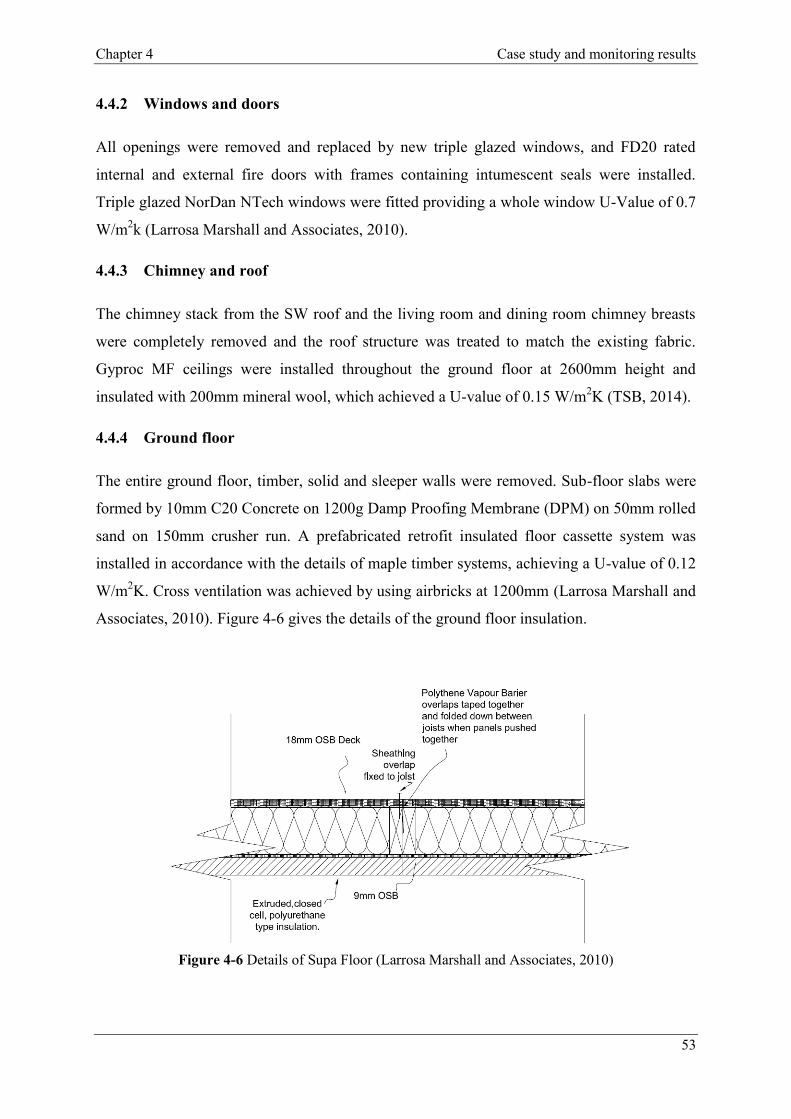
Chapter 4 Case study and monitoring results
53
4.4.2 Windows and doors
All openings were removed and replaced by new triple glazed windows, and FD20 rated
internal and external fire doors with frames containing intumescent seals were installed.
Triple glazed NorDan NTech windows were fitted providing a whole window U-Value of 0.7
W/m2k (Larrosa Marshall and Associates, 2010).
4.4.3 Chimney and roof
The chimney stack from the SW roof and the living room and dining room chimney breasts
were completely removed and the roof structure was treated to match the existing fabric.
Gyproc MF ceilings were installed throughout the ground floor at 2600mm height and
insulated with 200mm mineral wool, which achieved a U-value of 0.15 W/m2K (TSB, 2014).
4.4.4 Ground floor
The entire ground floor, timber, solid and sleeper walls were removed. Sub-floor slabs were
formed by 10mm C20 Concrete on 1200g Damp Proofing Membrane (DPM) on 50mm rolled
sand on 150mm crusher run. A prefabricated retrofit insulated floor cassette system was
installed in accordance with the details of maple timber systems, achieving a U-value of 0.12
W/m2K. Cross ventilation was achieved by using airbricks at 1200mm (Larrosa Marshall and
Associates, 2010). Figure 4-6 gives the details of the ground floor insulation.
Figure 4-6 Details of Supa Floor (Larrosa Marshall and Associates, 2010)

Chapter 4 Case study and monitoring results
54
4.4.5 Heating and hot water system
The heating system is a classic Passivhaus design where the heat recovery ventilation system
provides space heating as well as supply and extract ventilation. As a back-up strategy,
supplementary heating from the main gas-fired boiler feeding radiators has been
incorporated. Solar thermal panels were also installed to the South face of the rear roof to
provide domestic hot water supported by a gas condensing boiler. Figure 4-7 illustrates the
layout of mechanical services in the house (Larrosa Marshall and Associates, 2010).
Figure 4-7 layout of mechanical services (Larrosa Marshall and Associates, 2010)
4.4.6 MVHR
Although the building benefits from natural ventilation but all air paths were eliminated by
sealing the building and thermal bridges were minimised by continuous insulation, which
offers exceptionally good air-tightness, cuts heating demand and improves thermal comfort.
However, very low air leakage rates can lead to under-ventilation. Therefore, additional
ventilation provisions – as recommended in Part L of the Building Regulations 2013 ‒ were
applied, achieving 5 m3/m
2/hr@50pa (DCLG, 2013). At the time of the refurbishment (2010)
the technology for whole house Mechanical Ventilation with Heat Recovery (MVHR) system
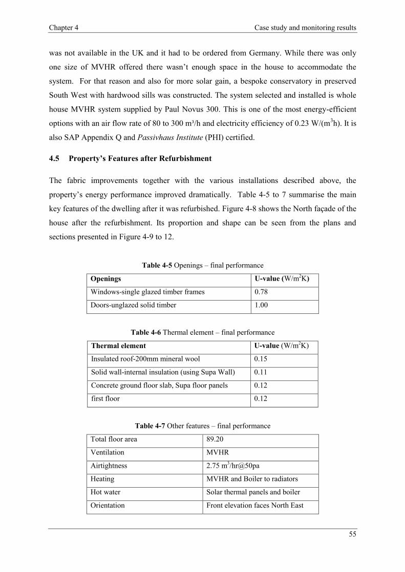
Chapter 4 Case study and monitoring results
55
was not available in the UK and it had to be ordered from Germany. While there was only
one size of MVHR offered there wasn’t enough space in the house to accommodate the
system. For that reason and also for more solar gain, a bespoke conservatory in preserved
South West with hardwood sills was constructed. The system selected and installed is whole
house MVHR system supplied by Paul Novus 300. This is one of the most energy-efficient
options with an air flow rate of 80 to 300 m³/h and electricity efficiency of 0.23 W/(m3h). It is
also SAP Appendix Q and Passivhaus Institute (PHI) certified.
4.5 Property’s Features after Refurbishment
The fabric improvements together with the various installations described above, the
property’s energy performance improved dramatically. Table 4-5 to 7 summarise the main
key features of the dwelling after it was refurbished. Figure 4-8 shows the North façade of the
house after the refurbishment. Its proportion and shape can be seen from the plans and
sections presented in Figure 4-9 to 12.
Table 4-5 Openings – final performance
Openings U-value (W/m2K)
Windows-single glazed timber frames 0.78
Doors-unglazed solid timber 1.00
Table 4-6 Thermal element – final performance
Thermal element U-value (W/m2K)
Insulated roof-200mm mineral wool 0.15
Solid wall-internal insulation (using Supa Wall) 0.11
Concrete ground floor slab, Supa floor panels 0.12
first floor 0.12
Table 4-7 Other features – final performance
Total floor area 89.20
Ventilation MVHR
Airtightness 2.75 m3/hr@50pa
Heating MVHR and Boiler to radiators
Hot water Solar thermal panels and boiler
Orientation Front elevation faces North East

Chapter 4 Case study and monitoring results
56
Figure 4-8 North façade (Gladwin, 2011)
Figure 4-9 North Façade (Larrosa Marshall and Associates, 2010)

Chapter 4 Case study and monitoring results
57
Figure 4-10 South Façade (Larrosa Marshall and Associates, 2010)
Figure 4-11 Ground floor plan (Larrosa Marshall and Associates, 2010)

Chapter 4 Case study and monitoring results
58
Figure 4-12 First floor plan (Larrosa Marshall and Associates, 2010)

Chapter 4 Case study and monitoring results
59
4.6 Refurbished House PHPP Report
The whole house modelling was undertaken in PHPP whose results indicate a 74% reduction
in CO2 emissions and 72% savings in energy bills (see Appendix C for the results and Figure
4-13 for the energy predictions). Predictions from the PHPP analysis suggested an annual
space heating demand of 29kWh/m2, which is much greater than the 15kWh/m
2 suggested as
a Passivhaus standard. The annual primary energy demand was estimated to be 102kWh/m2;
therefore, the house achieved the 120 kWh/m2
Passivhaus target. The total predicted CO2
post-refurbishment emissions was 20 kgCO2/yr. In summary, therefore, although energy
performance was dramatically improved the house did not reach a certifiable Passivhaus
standard.
Figure 4-13 PHPP predictions for 2 Broxton street energy performance
4.7 Costs of Refurbishment
The cost of providing energy efficiency measures ‒ wall, roof and floor insulation, replacing
doors and windows, low carbon technologies and building services ‒ was £61,260 and the
entire project cost £193,308 . See Table 4-8 for full details.
Specific Demands with Reference to the Treated Floor Area
Treated Floor Area: 89.2 m2
Applied: Monthly Method PH Certificate: Fulfilled?
Specific Space Heat Demand: 29 kWh/(m2a) 15 kWh/(m
2a) No
Pressurization Test Result: 1.0 h-1 0.6 h-1 No
Specific Primary Energy Demand(DHW, Heating, Cooling, Auxiliary and Household
Electricity):102 kWh/(m
2a) 120 kWh/(m2a) Yes
Specific Primary Energy Demand
(DHW, Heating and Auxiliary Electricity): 71 kWh/(m2a)
Specific Primary Energy Demand
Energy Conservation by Solar Electricity: kWh/(m2a)
Heating Load: 13 W/m2
Frequency of Overheating: 0 % over 25 °C
Specific Useful Cooling Energy Demand: kWh/(m2a) 15 kWh/(m2a)
Cooling Load: 4 W/m2

Chapter 4 Case study and monitoring results
60
Table 4-8 The cost breakdown of the project: data provided by Plus Dane Group
Item
Design Stage (£) Construction
Phase (£) Comments
Material Labour Material Labour
Design
24,814
24,814 Larrosa Marshall
Prelims 14,294
14,294
Fabric measures 12,000 4,000 12,000 7,000 PLB assist pf Maple
Building services
(Conventional) 9,050 1,650 9,050 2,500
Cost addition for parity wiring by
PLB
Low/zero carbon
technologies 6,160
6,560
MVHR and Solar Thermal spec
change
Renew roof 1,950 2,000 1,950 2,000
Triple glazing
and doors 18,200 2,000 18,200 2,000
Site preparation 57,400 5,000 57,400 1,500 Strip out and removal of asbestos
New
conservatory at
rear
2,800 1,200 2,800 1,200
Painting and
decorating 1,500 2,000 1,500 2,000
Other costs 24,240
21,090 43,014 Drainage, kitchen and bathroom
fittings, external works
Monitoring
equipment 5,450
5,450
Parity Projects
Chapter 4 Case study and monitoring results
61
4.8 Airtightness Test of the Refurbished House
Short-term monitoring of airtightness was carried out by BSRI. The final air leakage rate of
the dwelling was 2.7m3/m
2/h@50Pa ‒ equivalent to 1.0 ACH ‒ which is marginally above the
0.6ACH Passivhaus target although it meets the EnerPHit standard. Details of the test can be
seen in Appendix D.
4.9 Results – Long Term Monitoring
4.9.1 Monitoring system
Long-term measurements and assessments, compliant with the specification of the Energy
Saving Trust protocol, were carried out to evaluate the building’s performance. A wireless
data logging and monitoring system installed by Parity Projects in order to interfere as little
as possible with the lives of the occupants over the two years testing period. Since the
refurbished house was first occupied in November 2010, two complete years of monitored
data covering all parameters have been recorded at five minute intervals, providing the
following data:
1. External temperature and external relative humidity, measured by an external
thermistor sensor located at 1st floor level at front of the house (South).
2. Room temperature and relative humidity and concentration of CO2, measured in
the living room by a data logger mounted in the top corner of the part wall.
3. Internal temperature measured in the conservatory.
4. Utilities metering of electricity, gas and water consumption; detailed electricity
sub- metering on the following circuits: kitchen sockets, upstairs lights,
downstairs lights, upstairs sockets, downstairs sockets, and MVHR.
5. Air temperature of MVHR ducts measured by thermistors mounted on the supply
and extract duct of MVHR.
6. Floor, wall and ceiling surface temperatures and thermal gradients were measured.
7. Energy produced by solar thermal panel was quantified using a heat meter.
8. For the first year of occupancy the concentration of CO2 and the whole house
electricity and gas consumption were measured.
Because the data logger for the internal temperature was located on the top corner of the
living room it showed very high temperatures; consequently, readings from thermistor sensor

Chapter 4 Case study and monitoring results
62
in the side wall measuring temperatures inside insulation were used to evaluate internal
temperature.
4.9.2 Number of occupancy days and degree days
Table 4-9 compares 2011 and 2012 heating degree days for a base temperature of 15.5 0C.
The results show significant differences between 2011 and 2012 external temperature and
heating degree days. Also, diverse occupancy levels in 2011 and 2012 resulted in a
considerable discrepancy in the amount of energy used following refurbishment. Number of
occupancy days was calculated using monthly water consumption rates and un-structured
interviews. Hence, the results of energy consumption have been presented for each year
separately, while the 2011 and 2012 average energy consumption has been used for data
analysis and comparison. The number of occupancy days in the refurbished house during
2011 and 2012 can be seen in Table 4-10.
Table 4-9 Comparison of 2011 and 2012 Liverpool heating degree days for a base temperature of
15.50C (BizEE Software , 2013)
Time Jan Feb Mar Apr May Jun Jul Aug Sep Oct Nov Dec Total
2011 344 225 256 112 98 56 26 27 37 90 162 256 1689
2012 284 291 200 228 129 68 33 18 79 177 248 307 2062
Table 4-10 Comparison of the number of occupancy days in the refurbished house during 2011 and
2012
Time Jan Feb Mar Apr May Jun Jul Aug Sep Oct Nov Dec Total
2011 27 22 24 25 26 23 28 21 23 25 25 30 299
2012 28 24 27 26 30 29 28 24 28 30 28 31 333
4.9.3 Grid energy use
4.9.3.1 Gas
The average gas consumption during 2011 was 49kWh/m2, while in 2012 it was 71kWh/m
2.
With occupancy of two adults and two children (2.8) the per capita gas consumption was
1568kWh in 2011 and 2271kWh in 2012. This can be compared to the UK average based on
two recent studies of Low Carbon Hub (LCH) (Low Carbon Living Training, 2012) and one

Chapter 4 Case study and monitoring results
63
by Ofgem (Ofgem, 2011) which showed the typical average annual domestic gas usage to be
approximately 16500kWh/household, which is 90% more than the first year’s consumption
and 86% more than the second year’s consumption at the Broxton Street house. See Table
4-11.
A summary of month by month gas usage shows that over the two years the house consumed
60kWh/m2 gas energy for heating, for domestic hot water used as a back-up for solar
thermals, and for cooking. See Table 4-12.
Table 4-11 The UK average energy consumption per capita (Ofgem, 2011)
Fuel type level
current
consumption
figures
consumption
figures from 17
January
Difference in
reporting the
average DD bill
Gas (kWh)
low 10000 11000 £29
medium 20500 16500 -£116
high 28000 23000 -£145
Electricity:
Profile Class 1
(kWh);credit
meters
low 1650 2100 £53
medium 3300 3300 £0
high 4600 5100 £59
Electricity:
Profile Class 2
(kWh);multi
rate meters
low 3300 2900 -£38
medium 6600 5000 -£152
high 9900 8300 -£152
Table 4-12 Monthly gas consumption of the refurbished house (kWh)
Time Jan Feb Mar Apr May Jun Jul Aug Sep Oct Nov Dec
2011 1,109 749 575 75 80 45 14 42 68 197 486 950
2012 989 931 498 497 212 217 108 55 214 548 899 1192
4.9.3.2 Electricity
The total electricity consumption, for lighting, the central heat pump, the MVHR, appliance
socket loads and auxiliary loads, was 30kWh/m2 in 2011 and 29kWh/m
2 in 2012 (see Table

Chapter 4 Case study and monitoring results
64
4-13 for monthly usage) i.e. the per capita electricity consumption was 972kWh in 2011 and
923kWh in 2012. Given an average electricity usage of 948kWh/person over two years,
compared with the UK average of 3300kWh/person (see Table 4-11), 71% less electricity
was used in the Broxton Street house.
Table 4-13 Monthly electricity consumption of the refurbished house (kWh)
Time Jan Feb Mar Apr May Jun Jul Aug Sep Oct Nov Dec Total
2011 273 255 229 223 220 197 216 190 202 216 235 262 2721
2012 247 222 206 206 211 200 193 184 200 216 232 265 2584
4.9.3.3 Total grid energy used
The average gas and electricity consumption in the first and second years for the Broxton
Street house was 8028kWh ‒ or 90kWh/m2 per annum. The energy consumption of the new
build Camden Passivhaus, with 65kWh/m2 and the Princedale Road retrofit dwelling, with
62kWh/m2, are the lowest energy, small family dwellings monitored in the UK. Other low
energy monitored buildings are the BedZed development, with 90kWh/m2, the Long House,
with 80kWh/m2 and the Bioregional One Brighton apartments, with 72kWh/m
2 which are all
new developments (Ridley, et al., 2013). Therefore, the refurbished Broxton Street house in
Liverpool is ranked among the low energy houses in the UK. See Table 4-18 for the
breakdown of total energy use.
4.9.4 Total primary energy used
The primary energy consumption figure includes all energy used in the house, including that
for appliances (white goods) and consumer electronics. The PHPP primary energy factors of
1.10 for gas and 2.70 for electricity were assumed in order to calculate the primary energy
use for the Broxton Street house (Ian Ridley, 2013). As can be seen in Table 4-14 and Table
4-15, total primary energy demand was 136.5kWh/m2 in 2011 and 156.6kWh/m
2 in 2012.
Considering the average primary energy use of 146.6kWh/m2 for the house over two years,
this is 22% greater than the 120kWh/m2 target of the Passivhaus and EnerPHit standards.
However, TSB has used a primary energy factor of 1.00 for gas and 2.8 for electricity, which
gives an average primary energy use of 143.5kWh/m2, which is 25% greater than the
competition target of 115kWh/m2.

Chapter 4 Case study and monitoring results
65
Table 4-14 Primary energy use in the refurbished house in 2011
Type of energy used Grid energy use
(kWh/m2)
Primary energy
factor
Primary energy use
(kWh/m2)
Gas usage 2011 49.2 1.1 54.1
Electricity usage 2011 30.5 2.7 82.4
Table 4-15 Primary energy use in the refurbished house in 2012
Type of energy used Grid energy use
(kWh/m2)
Primary energy
factor
Primary energy use
(kWh/m2)
Gas usage 2012 71.3 1.1 78.4
Electricity usage 2012 28.9 2.7 78.2
4.9.5 CO2 emissions
The UK carbon intensity of 0.195kgCO2/kWh from gas and 0.422kgCO2/kWh from
electricity was assumed in order to estimate the CO2 emissions from the Broxton Street house
(Pout, 2001). The house emitted 22kgCO2/kWh.m2 in the first year and 26kgCO2/kWh.m
2 in
second year. Table 4-16 and Table 4-17 show the carbon emissions from different fuel usage
in both years of occupancy. Thus, an average of 24kgCO2/kWh.m2 per year has been emitted
since its occupancy. TSB uses the same factors to calculate carbon emissions; therefore, the
amount achieved by Plus Dane Group is 42% higher than the competition target of
17kgCO2/kWh.m2.Compared with the average UK CO2 emissions per household in 2009 of
5500kg, emissions from the house were 85% less CO2 per capita (Palmer and Cooper, 2012).
See Table 4-18 for the breakdown of CO2 emissions from different usages.
Table 4-16 Carbon emissions from different gas and electricity usage in refurbished house in 2011
Type of energy used Grid energy use
(kWh/m2)
Emission factor
(kgCO2/kWh)
Primary energy use
(kgCO2/kWh.m2)
Gas usage 2011 49 0.195 9
Electricity usage 2011 30 0.422 13

Chapter 4 Case study and monitoring results
66
Table 4-17 Carbon emissions from different gas and electricity usage in refurbished house in 2012
Type of energy used Grid energy use
(kWh/m2)
Emission factor
(kgCO2/kWh)
Primary energy use
(kgCO2/kWh.m2)
Gas usage 2012 71 0.195 14
Electricity usage 2012 29 0.422 12
Table 4-18 Breakdown of total energy use and CO2 emissions
Energy use 2011 energy
use (kWh)
2012 energy
use (kWh)
2011 CO2
emissions
(kgCO2/yr)
2012 CO2
emissions
(kgCO2/yr)
Space heating (gas) 3999 5562 779 1085
Kitchen socket (electricity) 1341 1289 566 544
Appliance socket loads (electricity) 659 573 278 242
Auxiliary loads (electricity) 316 297 133 125
DHW (gas) 391 798 76 155
Central heat pump (electricity) 142 184 60 77
Lighting (electricity) 133 106 56 45
MVHR (electricity) 130 134 55 56
4.9.6 DHW and solar thermal panels
The electricity required for domestic hot water (DHW) in 2011 was 1319kWh and in 2012
1681kWh. Solar thermal panels provided 70% ‒ 928kWh ‒ of the hot water required in 2011
and 53% ‒ 883kWh ‒ in 2012. Table 4-19 give monthly details of DHW requirement and its
source for each year.
4.9.7 Comfort and indoor air quality
To assess the level of occupant’s comfort after refurbishment, internal temperature, humidity
and CO2 concentration has been measured in the living room.

Chapter 4 Case study and monitoring results
67
Table 4-19 monthly details of DHW requirement and its source for each year
Time
Total Hot water
requirement for
2011
(kWh)
Of which
provided by solar
thermal panels in
2011
(kWh)
Total Hot water
requirement for
2012
(kWh)
Of which
provided by solar
thermal panels in
2012
(kWh)
Jan 111 28 146 41
Feb 111 39 128 49
Mar 138 86 178 122
Apr 144 134 159 97
May 108 99 170 140
Jun 120 116 127 94
Jul 132 131 125 109
Aug 94 89 125 117
Sep 98 90 87 57
Oct 83 64 112 30
Nov 73 34 146 17
Dec 107 18 178 10
Total 1319 928 (70%) 1681 883 (53%)
4.9.7.1 Temperature
The average internal temperature in the living room was 19.70C during the heating season ‒
October 2011 to March 2012 ‒ when the mean external temperature was 9.6oC. During the
cooling season ‒ April 2011 to September 2011 ‒ the mean internal temperature was 22.60C
with the external average temperature of 15.40C. The CIBSE recommended comfort criteria
is 22-230C for living rooms in winter with 1.0 clothing level and 23-25
0C during summer
with 0.65 clothing level (CIBSE, 2006).Although the standard deviation ‒ the dispersion of a
set of data ‒ of 2011 external temperature was 4.3%, internal temperatures change in 1.7%.
Table 4-20 and Table 4-21 compare the monthly mean internal temperatures in the house
after refurbishment against the measured external temperature.

Chapter 4 Case study and monitoring results
68
Table 4-20 Comparison of variations in the monthly mean internal temperatures in the house after
refurbishment against measured external temperature for heating season
Heating season Oct
2011
Nov
2011
Dec
2011
Jan
2012
Feb
2012
Mar
2012 Average
Standard
deviation
Mean monthly
internal
temperature
21.2 19.3 18.8 18.9 19.1 20.9 19.7 0.9
Mean monthly
external
temperature
13.2 9.9 5.5 8.3 8.4 12.4 9.6 2.6
Table 4-21 Comparison of variations in the monthly mean internal temperatures in the house after
refurbishment against measured external temperature for heating season
Cooling season Apr
2011
May
2011
Jun
2011
Jul
2011
Aug
2011
Sep
2011 Average
Standard
deviation
Mean monthly
internal
temperature
21.5 21.6 22.9 23.7 23.1 22.9 22.6 0.6
Mean monthly
external
temperature
12.9 13.5 15.9 17.4 16.7 15.8 15.4 1.6
4.9.7.2 Overheating
The CIBSE suggests 250C as an acceptable summer indoor design operative temperature for
living rooms and it also recommends restraining the estimated incidence of operative
temperatures above 280C to 1% of the annual occupied period ‒ i.e. around 25–30 hours per
year (CIBSE, 2006). During 2011, the highest indoor temperature, on 31 July, was 26.5 and,
at 1.9%, the annual operative temperature was over 250C. Figure 4-14, which compares the
peak internal temperature on 31 July with the external temperature at the same time, shows
that, although the external temperature indicated a standard deviation of 2.3%, the internal
temperature deviated by 0.41%. In 2012 the highest operative temperature was 26.3 on 8
September and 4.4% of the annual measured operative temperature was over 250C.

Chapter 4 Case study and monitoring results
69
Figure 4-14 Comparison of internal and external mean temperature in in 31 of July (peak time)
4.9.7.3 Humidity
Both low humidification in cold dry winter conditions and high relative humidity (RH) in
warm temperature for naturally or mechanically ventilated buildings could have a harmful
effect on health. Consequently, CIBSE has considered 40-70% RH range as an acceptable
normal standard, with 65% as being comfortable (CIBSE, 2006). Table 4-20 shows two years
of monthly internal humidity measurements using a sensor mounted on the top corner of the
internal surface of the West external wall, which shows that most of the times the internal
humidity is below the CIBSE approved 40-70% RH norm. Figure 4-15 shows that during
2011, when this data was compared with external temperature and humidity, changes in
internal RH were not effected by the external temperature.
Table 4-22 Comparison of mean monthly internal for the house after refurbishment
Measure Jan Feb Mar Apr May Jun Jul Aug Sep Oct Nov Dec
Internal
Humidity-
2011
33 36 34 36 35 36 37 39 41 41 41 36
Internal
Humidity-
2012
36 34 35 34 36 40 41 41 41 40 37 35
0
5
10
15
20
25
30
00:0
0
01:0
0
02:0
0
03:0
0
04:0
0
05:0
0
06:0
0
07:0
0
08:0
0
09:0
0
10:0
0
11:0
0
12:0
0
13:0
0
14:0
0
15:0
0
16:0
0
17:0
0
18:0
0
19:0
0
20:0
0
21:0
0
22:0
0
23:0
0
External Temperature Internal temperature

Chapter 4 Case study and monitoring results
70
Figure 4-15 Comparison of the changes in internal humidity with internal temperature and external
humidity with for the first year of occupancy (2011)
4.9.7.4 CO2 concentration
CO2 concentration in the living room was measured from December 2010 to October 2011.
The monthly average of the captured data can be seen in Table 4-23. CO2 emissions were
measured in living room during the occupied hours -7:30am-11:30am and 16:00-22:30- by an
air quality indicator in order to evaluate the level of indoor air pollution (BSI, 2008). In the
UK, CO2 levels of between 800 to 1000PPM indicate an appropriate ventilation rate, which
equates to a fresh air ventilation rate of 8l/s per person (CIBSE, 2005) (see Table 4-24).
Indoor levels of CO2 exceeded 1000PPM for 340 hours, or 11% of the time when the house
was occupied in the first year of monitoring. However, the house design meets IDA3 rather
than IDA2 – good, CO2<1000PPM – which ensured that RH levels in winter were not too
low, i.e. below 30%. Indoor levels of CO2 exceeded 1200PPM for only 77 hours, or 2.5% of
the time under the same conditions. See Table 4-25 for more details.
Table 4-23 Monthly average of the captured CO2 concentration during occupied hours
Measure Dec
2010
Jan
2011
Feb
2011
Mar
2011
May
2011
Apr
2011
Jun
2011
Jul
2011
Aug
2011
Sep
2011
Oct
2011
CO2
concentration 890 836 822 803 782 732 663 648 794 719 680
0
5
10
15
20
25
0
10
20
30
40
50
60
70
80
90
100
Jan Feb Mar Apr May Jun Jul Aug Sep Oct Nov Dec
Inte
rnal
tem
per
ature
(0C
)
Inte
rnal
hum
idit
y (
%)
Internal Humidity-2011 External Humidity-2011 Internal Temperature-2011

Chapter 4 Case study and monitoring results
71
Table 4-24 Recommendations for appropriate ventilation rate (Taylor and Morgan, 2011)
Carbon dioxide CIBSE Guide B, 2005 ASHRAE
Outside air Approx. 350PPM Approx. 350PPM
As an indicator of adequate air
quality 800-1000PPM
under 1000PPM
As a pollutant 5000PPM (8 hours av.) 2500PPM
Table 4-25 Indoor levels of CO2
Time hrs>1000PPM %hrs>1000PPM hrs>1200PPM %hrs>1200PPM
Dec 2010 41 15 % 10 4 %
Jan 2011 55 19 % 13 5 %
Feb 2011 51 18 % 12 4 %
Mar 2011 21 7 % 3 1%
Apr 2011 40 14 % 13 5 %
May 2011 35 12 % 6 2 %
Jun 2011 20 7 % 2 1 %
Jul 2011 9 3 % 2 1 %
Aug 2011 16 6 % 5 2 %
Sep 2011 34 12 % 6 2 %
Oct 2011 18 7 % 5 2 %

Chapter 4 Case study and monitoring results
72
4.9.8 Broxton street house occupant’s feedback and energy bills
TSB estimated the annual energy bills of 2.63£/m2/yr for gas and £4.29£/m
2/yr for electricity
(TSB, 2013). The Department of Energy and Climate Change (DECC) has estimated the
average domestic energy price for different cities by assuming an annual gas consumption of
18000kWh and an annual electricity consumption of 3300 kWh (DECC, 2014d; DECC,
2014e). The annual gas bill for the Broxton Street house has been 70% lower and the
electricity bills have been 24% lower than an average house in Liverpool, which means that
the annual energy cost is 52% lower than the UK average. Table 4-26 and Table 4-27 show
the estimated prices by DECC. More details of costs, savings and payback time will be
discussed in Chapter 6.
Table 4-26 Average annual domestic gas bills in 2012 for Liverpool with average unit costs (DECC,
2014d)
Payment type Credit Direct debit Prepayment
Overall
(Pence per kWh and
pounds)
Town/city Bill range Unit
Cost Bill
Unit
Cost Bill
Unit
Cost Bill
Unit
Cost Bill
Liverpool
Largest 4.84 871 4.84 871 4.84 871
4.42 795 Average 4.62 832 4.25 766 4.60 827
Smallest 4.32 778 4.01 722 4.35 783
Table 4-27 Average annual domestic electricity bills in 2012 for Liverpool with average unit costs
(DECC, 2014e)
Payment type Credit Direct debit Prepayment
Overall
(Pence per kWh and
pounds)
Town/city Bill range Unit
cost Bill
Unit
cost Bill
Unit
cost Bill Unit cost Bill
Liverpool
Largest 17.89 590 15.81 522 16.39 541
15.24
503
Average 16.15 533 14.61 482 15.63 516
Smallest 14.30 472 13.08 432 14.89 491

Chapter 4 Case study and monitoring results
73
4.10 PHPP Results Compared to Monitoring Results
The Passivhaus Planning Package (PHPP) was used as the certification tool for the house
(see Section 4.6). Table 4-28 compares the PHPP results with the average results from
measured data during two years of monitoring. Substantial differences can be observed
between predicted and real performance, the reasons for which being that a Manchester
weather file was used for the weather estimations, together with unrealistic assumptions
being made regarding, (i) internal heat gains, (ii) interior comfort temperatures, (iii) the
efficiency of appliances, (iv) the use of shading devices, and (v) fabric heat loss. The
adjustment of these PHPP data based on monitoring outcomes could lead to more realistic
results. This will be discussed in more details in Chapter 5.
Table 4-28 comparison of PHPP results with real monitoring data
Measurement
method
Space
Heating
(kWh/m2/yr)
Primary
Energy Use
(kWh/m2/yr)
CO2
Emissions
(kg/m2/yr)
Overheating
(% over 25oC)
Total Fuel
Cost
(£)
PHPP 29 102 20 0 279
Monitoring 54 146 24 2 617
4.11 Analysing the Monitored Data
Despite the 2 Broxton Street Liverpool project failing to meet Passivhaus, EnerPHit and
‘Retrofit for the Future’ targets, the retrofitted house uses 60% less energy and produces 76%
fewer CO2 emissions than the estimated figures for a pre-refurbished house by TSB. The
house also saves approximately 60% in energy bills. In addition, its primary energy use of
146kWh//m2/yr is 13% lower than 169kWh/m
2/yr primary energy use of an EnerPHit
certified house in London – i.e. the Princedale Road Passivhaus. Furthermore, monitoring
results and occupant’s feedback all indicate that these saving were achieved while providing
a comfortable indoor thermal environment.
As mentioned previously, the house was a solid walled structure that was considered “hard to
treat”. From the eighty-six funded projects for the ‘Retrofit for the Future’ competition,
thirty-seven were analysed, out of which only twelve were terraced houses with solid walls.
Comparing these refurbished terraced houses with the Liverpool house shows that only three

Chapter 4 Case study and monitoring results
74
of these refurbished houses could save more CO2 emissions. In terms of primary energy use,
the Broxton Street house attained fifth place with only two houses in London achieving a
better airtightness level. Table 4-29 compares the performances of all the solid walled
terraced houses refurbished under ‘Retrofit for the Future’ competition.
These figures demonstrate that the performance of the refurbished Broxton Street Liverpool
house can contribute a great deal both to shaping how to deal with the UK’s existing housing
stock and showing what can be achieved through refurbishing similar period dwellings.
Table 4-29 Performance of all analysed solid wall terraced houses refurbished under ‘Retrofit for the
Future’ competition (EST, 2013)
Property
Type and age Location
Gross
Internal Area
(m2)
CO2
Emissions
(kgCO2/m2)
Airtightness
(m3/m
2/hr@50
pa)
Primary
Energy Use
(kWh/m2)
End Terraced
1986
Liverpool,
Merseyside 89.2 24.0 2.8 146.0
End Terraced
1945-1965
Rotherham,
South
Yorkshire
79.5 13.93 6.16 90.87
Mid Terraced-
pre 1900
London,
South East 114.6 20.6 0.3 136.5
Mid Terraced-
pre 1900
Clapham,
London 155.5 21.9 5.9 128.9
End Terraced
1950-1966
Rotherham,
South
Yorkshire
203.3 25.0 5.9 137.7
Mid-terraced-
1950-1966
Tower
Hamlet,
London
96.2 36.5 1.8 219.4
Mid Terraced-
1900-1929
Wakefield,
West
Yorkshire
196.9 38.9 4.4 228.1

Chapter 4 Case study and monitoring results
75
Mid Terraced-
pre 1900
Colne,
Lancashire 88.8 42.6 4.2 282.8
Mid Terraced-
1900-1929
Sea Palling,
Norfolk, 86.7 43.5 8.1 288.8
Mid Terraced-
pre 1900
Stoke-On-
Trent,
Staffordshire
64.0 46.8 4.3 284.4
Mid Terraced-
1950-1966
Rotherham,
South
Yorkshire
203.3 47.7 6.4 284.8
Mid Terraced-
pre 1900
Tower
Hamlet,
London
245.6 47.7 8.9 283.1
Mid Terraced-
1900-1929
Wakefield,
West
Yorkshire
215.8 50.6 3.2 323.5
4.12 Lessons and Challenges
Refurbishment and monitoring of the house at 2 Broxton Street in Liverpool revealed a
number of new challenges. Innovative solutions were therefore developed by Plus Dane
Group in order to manage and overcome them. One of the main challenges mention by
Martin Gladwin ‒ owner and chief executive of the project ‒ was interior wall insulation and
also ground floor insulation, which required the house to be empty. The second major
problem was the cost of the project, which was much higher than predicted. These two issues
will be highly significant if the findings are going to be rolled-out to the wider housing
market. Martin Gladwin says that working closely with the occupants is crucial and that the 2
Broxton Street tenants were involved both from the start and throughout the refurbishment
period. This engagement, alongside the training provided to help resident understands how to
maximise the benefits from the new technologies and renewable energy sources, enhanced
the effectiveness of the project.
The analysis derived from this 19th century terraced house refurbished project to near
‘Passivhaus’ standards, as presented in this chapter, gave a good indication of how to deal

Chapter 4 Case study and monitoring results
76
with the existing housing stock, whilst, at the same time, complying with conservation area
limitations. The study also revealed the extent to which CO2 reduction targets can be
achieved through refurbishing old housing stock, using existing technologies and practices.
The monitoring data derived from the energy consumed in the house was captured during
2011 and 2012. Overall, the analysis shows that it is possible to achieve sharp CO2 emissions
decline and large energy savings in a 130 years old house. However, due to different
occupancy levels and of the fluctuations of temperatures over each year, there is a significant
difference in results. Accordingly, great care must be taken not to overstate the results from
one, or even two years of data. Hence, in order to assess and produce a comprehensive
performance study, several cases under different climatic conditions should be obtained.
In addition to more detailed occupancy and external temperature records, extra care should be
taken in regard to the captured data. For instance, in this case study some problems were
experienced with the MVHR and internal temperatures. For instance, some measurement data
were only available for the first year of monitoring, such as internal CO2 concentrations and
external temperatures.
This, and other studies, demonstrates a great dissimilarity between predicted and monitored
values; they can, thus, help to normalise the input data in the relevant software packages. The
terraced house investigated in this study has survived for over a hundred years; therefore it is
very likely that the renovation work will ensure that it survives for at least another fifty. The
next chapter of this thesis will use thermal simulation software, DesignBuilder and future
weather data files in order to examine the impact of climate change on this dwelling’s future
energy demands, CO2 emissions and internal comfort conditions

Chapter 5 – Dynamic Thermal Modelling and Future
Performance
5 Not erase
Not erase

Chapter 5 Dynamic thermal modelling and future performance
76
5.1 Chapter Overview
The main focus for previous chapter has been to assess the short-term mitigation potential and
effectiveness of adaptation refurbishment measures in meeting the UK’s 2050 climate change
target for a refurbished terraced house in Liverpool.
In this chapter the impact of climate change for the period up to 2080 has been projected in terms
of internal temperatures and energy use. The long-term vulnerabilities and capabilities of
adaptation measures, energy and carbon performances are also examined by modelling the
building and by using probabilistic UK future weather data in the DesignBuilder thermal
simulation software tool. Also, the actual values obtained from the monitoring records have
assisted in normalizing the software input data in order to achieve more accurate model and
results. Hence this chapter will report on the reliability of DesignBuilder by illustrating how
different parameters in modelling will impact on the accuracy of the final results.
Results reflect the necessity of considering either a cooling system or modifications in design –
or both – to the pre and post-refurbished house to meet acceptable internal conditions in the
future; they will also demonstrate that, although the heating demand shows a decreasing trend
over the century, the effect of refurbishment on reducing the heating requirement will be much
higher than the effect of climate change.
5.2 Buildings and Climate Change
As mentioned previously, the built environment is a substantial contributor to anthropogenic –
the main cause of climate change – greenhouse gas emissions to which buildings in developed
nations contribute between 25% and 40% (Dimoudi and Tompa, 2008; Gustavsson, Joelsson and
Sathre, 2010). Because a building’s performance is directly affected by the climate to which it is
exposed, its lifespan of between fifty to a hundred years is consistent with the timescale during
which predictably substantial climate changes will occur (de Wilde and Coley, 2012). Therefore,
this chapter will examine the resilience of buildings and the internal and external modifications
and adaptations they will require if their service lives are to continue in the face of such climatic
change.

Chapter 5 Dynamic thermal modelling and future performance
77
To predict annual energy consumption, assess the adequacy of natural ventilation and estimate of
the cooling capacity that will need to be provided through a building’s life span, designers need
to model its future thermal performance. In order to achieve such long-term assessments,
computer-based modelling techniques and future weather files are essential (Levermore, et al.,
2012). Two principle challenges must be faced when adopting such a modelling method: (i)
discrepancies that may occur between predicted and real performance due to human behaviour
must be factored in, and (ii) the uncertainties in projections of climate change, which cannot be
validated since they do not relate to replicable events (Guan, 2009; de Dear, 2006). This chapter,
therefore, will suggest a sensitivity analysis framework for model validation and the selection of
weather files in order to reduce the impact of these uncertainties and discrepancies when
predicting the performance of buildings. For the purpose of this research, dynamic thermal
simulation software, DesignBuilder (DB), and Exeter University EPW weather files will be used
to examine future performance of the cases studied in this research. The selection of cases was
principally aimed to deal with uncertainties and also what has been termed the “performance
gap” (see 5.3 below). The process adopted in these selections will be described later in this
chapter. Figure 5-1 summarizes the steps of analysis for estimating future performance of the
post and pre-refurbished house, including a summary of results at each step. The aim was to
create a validated model in DesignBuilder by selecting the most effective range of weather files
in order to predict the future performance of the refurbished house in terms of several different
levels of climate change probabilities.
5.3 Modelling and Model Calibration Methodology
Computer-based modelling and simulation is commonly held to be the best practice approach to
not only estimating the operational energy performance of buildings at the design stage, but also
predicting its future performance when integrated with future weather files. However, there are
significant contradictions between simulated results and real outcomes. Though, selecting a
reliable tool for analysis and normalising the computer models by means of measured data can
reduce this discrepancy – commonly referred to as the “performance gap”.

Chapter 5 Dynamic thermal modelling and future performance
78
Figure 5-1 Steps of modelling and evaluating future performance of a pre and post refurbished terraced
house in Liverpool

Chapter 5 Dynamic thermal modelling and future performance
79
Several studies, such as PROBE (Post-occupancy Review of Buildings and Engineering) and
CarbonBuzz have investigated and reported this gap (Leaman, n.d.). For most non-residential
buildings, computer models underestimate required energy, while two residential case studies by
CarbonBuzz – the ‘Parity Projects Demo House’ and ‘Ford Farm’– overestimated energy
consumption in their computer models by 72% and 36% respectively (CarbonBuzz, 2014a;
CarbonBuzz, 2014b).
In all these cases, though, lack of feedback regarding actual attempts to standardise the
benchmarks and an inability to model occupancy schedules have been pointed out as the
underlying causes of these discrepancies (Menezes , et al., 2012).
In view of this significant “performance gap” DesignBuilder was selected for modelling and
evaluating the future performance of the case study house, since it has proved to be the most
inclusive interface to EnergyPlus – the most advanced building simulator – which has been the
subject of extensive validation through an ongoing U.S. Department of Energy (DOE)
development and support programme (EERE, 2014). Schedule and occupancy definition options
in the software allow users to, (i) produce more accurate models (ii) model and simulate
advanced building systems, (iii) define components in great detail, (iv) present flexible results
due to its ability to switch between zones, (v) account for seasonal conditions, and (vi) produce
annual and sub-hourly results ( Mustafaraj , et al., 2014; Yiqun , et al., 2011).
DesignBuilder is capable of modelling the impact of occupancy, heat gain and building
operational schedules in detail. Having post-occupancy measured data from extensive
monitoring helped to create an accurate model of the case study house.
To illustrate the extent of the discrepancy between predicted and actual measures - in particular
for residential building estimations the model was developed over four stages, (i) modelling
based on “as built” information, (ii) calibrating the model based on walkthrough and un-
structured interviews, (iii) calibrating the model based on long-term measured data, and (iv)
updating the model based on available benchmarks. By this means, an evidence-based calibration
methodology by Bertagnolio has been employed and developed by author of this thesis for
calibration of the model (Bertagnolio , 2012). Figure 5-2 depicts the methodology for the present
research.

Chapter 5 Dynamic thermal modelling and future performance
80
Figure 5-2 Modelling and calibration methodology
5.3.1 Stage 1–Modelling based on “as built” information
Stage 1-1: 3D model of the refurbished house
The two story 89.2 m2 refurbished 19th century end-terraced house was modelled in a five stage
process using DesignBuilder, (i) the geometry of the building was derived from the architectural
drawings, (ii) the gross internal floor-plan area was created in AutoCAD drawings (DWG), (iii)
the file was imported into DesignBuilder, (iv) the model was created by tracing over the
imported plans, (v) a series of individual zones, based on the different thermal characteristics of
the rooms, was created, and (vi) the appropriate activity was assigned to each zone to define the
treated floor area. Figure 5-3 and Figure 5-4 give a 3D view as generated by DesignBuilder.

Chapter 5 Dynamic thermal modelling and future performance
81
Figure 5-3 DB generated model-rear facade
Figure 5-4 DB generated model-front facade
Stage 1-2: Input “as-built” variables to the model
As the detailed information on construction, opening, type of lighting and HVAC became
available, the parameters were modelled and adjusted to the 3D model without making any
assumption. Details of stages 1-2 input data can be seen in Chapter 4, Section 4.5. Table 5-1
compares the actual post refurbishment thermal features of the house with the modelled features
in DesignBuilder.
Assumed input data provided by DesignBuilder was used are as follow (i) occupancy density, (ii)
activity and metabolic factors, (iii) number of holidays – i.e. absences from house, (iv) lighting
usage, (v) energy usage of kitchen sockets and other equipment, (vi) catering energy use, (vii)
consumption rate for domestic hot water, (viii) schedules for heating, lighting and occupancy,
and (ix) set-point temperature. These parameters were not changed in the first stage as they are
causal and mostly dependant on how the building is run and maintained by the occupants, rather
than by its design and construction.
Stage 1-3: Simulation and comparison of calculated and real performance
A current EPW file of Liverpool was used for the simulation. All treated zones assumed by
DesignBuilder to be kept to a nominal set point temperature of 210C and heated to set points of
between 180C and 21
0C, depending on the nature of usage.

Chapter 5 Dynamic thermal modelling and future performance
82
Table 5-1 Compares real and modelled construction information
Thermal element Real U-value (W/m2K)
Modelled U-value
(W/m2K)
Insulated roof-200mm mineral wool 0.15 0.15
Solid wall-internal insulation (using Supa Wall) 0.11 0.11
Concrete ground floor slab, Supa floor panels 0.12 0.13
first floor 0.12 0.11
Windows-single glazed timber frames 0.78 0.78
Doors-unglazed solid timber 1.00 0.75
Table 5-2 compares the predicted results by DesignBuilder with the average actual performance
of the house, as measured during 2011 and 2012. Also a comparison of the monitoring results
was made using the results from other energy audit packages SAP and PHPP which were utilised
by the Plus Dane Group to predict performance after refurbishment. These are illustrated in
Figure 5-5.
The results represent a more accurate output, in terms of space heating requirement and primary
energy use, from DesignBuilder than the other two tools - SAP and PHPP – used, while PHPP
showed a more matching estimated energy use for lighting and water heating. For the refurbished
house, significant discrepancies between SAP predicted results and the actual measured
consumption can be seen in all measures. The most significant inconsistency between
DesignBuilder and actual output results was in lighting, which was predicted to be 85% above
the average lighting energy monitored in the house during two years of occupancy.
DesignBuilder estimated the water consumption to be 24% below the actual operational energy
performance, while its estimated primary energy use, which shows only a 5.8% underestimation,
is a good representative of actual performance. The space heating requirement prediction,
however, was 17% higher than the actual usage.
To standardise the model, and also to realise the magnitude of the effect of each parameter of the
simulated results, the causal parameters, which mostly relates to the occupants’ behaviour and
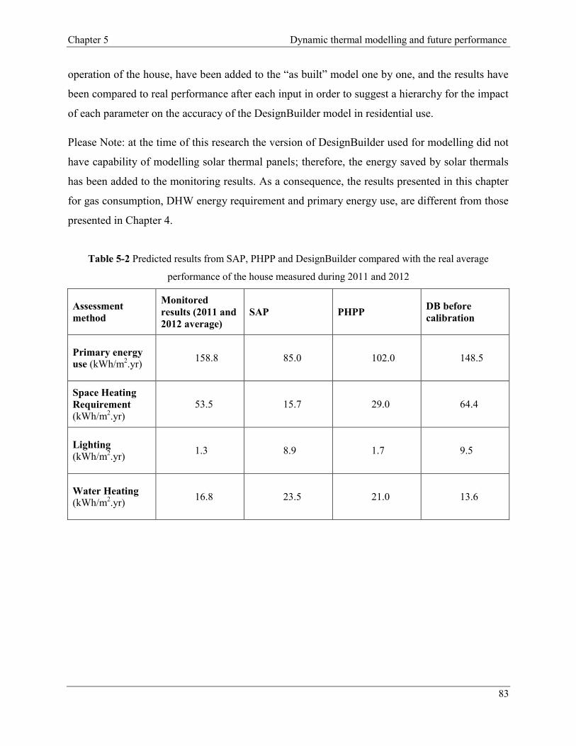
Chapter 5 Dynamic thermal modelling and future performance
83
operation of the house, have been added to the “as built” model one by one, and the results have
been compared to real performance after each input in order to suggest a hierarchy for the impact
of each parameter on the accuracy of the DesignBuilder model in residential use.
Please Note: at the time of this research the version of DesignBuilder used for modelling did not
have capability of modelling solar thermal panels; therefore, the energy saved by solar thermals
has been added to the monitoring results. As a consequence, the results presented in this chapter
for gas consumption, DHW energy requirement and primary energy use, are different from those
presented in Chapter 4.
Table 5-2 Predicted results from SAP, PHPP and DesignBuilder compared with the real average
performance of the house measured during 2011 and 2012
Assessment
method
Monitored
results (2011 and
2012 average)
SAP PHPP DB before
calibration
Primary energy
use (kWh/m2.yr)
158.8 85.0 102.0 148.5
Space Heating
Requirement
(kWh/m2.yr)
53.5 15.7 29.0 64.4
Lighting
(kWh/m2.yr)
1.3 8.9 1.7 9.5
Water Heating
(kWh/m2.yr)
16.8 23.5 21.0 13.6

Chapter 5 Dynamic thermal modelling and future performance
84
Figure 5-5 Comparison of average monitoring results and simulated estimates from DesignBuilder
5.3.2 Stage 2–Model calibration-modifying human factor parameters based on
walkthrough and unstructured interviews
Stage 2-1: Impact of occupancy density (Model 1)
The normalizing occupancy density of the DB model significantly impacted on, and reduced, the
predicted space heating requirement (gas), although it did not change the water consumption,
water heating energy requirement and lighting energy consumption. Therefore, changing this
parameter in DesignBuilder for a domestic building will only effect the space heating
requirements. Figure 5-6 illustrates the space heating requirement after the occupancy density
has been changed to an actual amount of 0.045people/m2
for the 89.2 m2 case study house with
four occupants.
Stage 2-2: Number of holidays (Model 2)
Modifying the number of holidays taken by the occupants impacted all parameters except the
lighting and DHW energy requirement. Figure 5-7 shows the comparison between the space
heating requirement (gas) before and after changing the number of holidays entered into the
0
50
100
150
200
250
Monitoring DB before calibration
kW
h/m
2.y
r
Space Heating Requirement Primary energy use Lighting Water Heating

Chapter 5 Dynamic thermal modelling and future performance
85
DesignBuilder model based on actual figures. Changes in electricity consumption can be seen in
Figure 5-8.
Figure 5-6 Space heating requirement after changing occupancy density to a real amount of
0.045people/m2
Figure 5-7 Comparison between space heating requirement before and after changing number of holidays
in DB with real measures
53.5
71.5
63.9
0 10 20 30 40 50 60 70 80
Actual
As-built model
Model 1
kWh/m2.yr
53.5
63.9
64.4
0 10 20 30 40 50 60 70
Actual
Model 1
Model 2
kWh/m2.yr

Chapter 5 Dynamic thermal modelling and future performance
86
Figure 5-8 Comparison between electricity requirement before and after changing the number of
holidays in DB with real measured data
5.3.3 Stage 3–Modelling and modifying causal parameters based on long-term monitoring
Stage 3-1: Water consumption (Model 3)
Even after normalizing the occupancy density and number of occupied days in DesignBuilder,
the results show a large discrepancy between actual and estimated DHW energy requirement.
The amount of water consumption was 0.7 l/m2-day by default, however, based on the
monitoring data, it can be modified. During 2011 and 2012, 3.30 l/m2-day and 3.60 l/m
2-day,
respectively, was the measured water consumption in the refurbished house. The monitored
energy use for DHW and the result of simulation after normalizing water use is presented in
Figure 5-9.
Stage 3-2: Set-point temperature (Model 4)
The minimal set-point temperature of 18 to 210C was considered by DesignBuilder. Undoubtedly
normalizing this parameter, based on real monthly mean internal temperatures, had a significant
impact on space heating consumption. The mean monthly internal temperature in the house has
been measured to be in the range of 21-25 0C during occupied hours. The graph presented in
30.2
26.5
26.8
24 25 26 27 28 29 30 31
Actual
Model 1
Model 2
kWh/m2.yr

Chapter 5 Dynamic thermal modelling and future performance
87
Figure 5-10 illustrates the effect of changing the set point temperature on heating consumption
and model validation.
Figure 5-9 Comparison between DHW energy requirement (gas) before calibration, the monitored energy
use for DHW and the result of simulation after normalizing water use
Figure 5-10 Impact of changing set point temperature on heating consumption (gas) and model validation
16.8
12.6
20.7
0 5 10 15 20 25
Actual
Model 2
Model 3
kWh/m2.yr
53.5
64.4
69.4
0 10 20 30 40 50 60 70 80
Actual
Model 3
Model 4
kWh/m2.yr

Chapter 5 Dynamic thermal modelling and future performance
88
Stage 3-3: Kitchen sockets, appliance socket loads and auxiliary loads heat gains (Model 5)
A comparison of monitored and predicted annual electricity consumption by kitchen sockets,
appliance socket loads and auxiliary loads can be seen in Table 5-3. After normalizing the input
data relating to the occupancy density and number of occupied days, the minimum amount of
937kWh (10kWh/m2) was assumed for interior equipment electricity use. The average monitored
measures, however, shows the considerably higher amount of 2237kWh. Changing this input
data not only had a significant impact on electricity consumption, but heat gain from these
consumptions resulted in reducing the space heating consumption by 12%. Figure 5-11 and
Figure 5-12 illustrate the impact of this change on the predicted space heating and electricity
requirement respectively.
Table 5-3 Comparison of monitored and predicted annual electricity consumption by kitchen sockets,
appliance socket loads and auxiliary loads
2011 energy use(kWh) 2012enenrgy use(kWh)
Kitchen socket (electricity) 1341 1289
Appliance socket loads (electricity) 659 573
Auxiliary loads (electricity) 316 297
Total (kWh) 2316 2159
Total (kWh/m2) 26 24
Total Predicted interior equipment
electricity use by DB 937kWh or 10.5kWh/m
2

Chapter 5 Dynamic thermal modelling and future performance
89
Figure 5-11 Comparison of space heating requirements (gas) predicted by DB before and after calibration
with monitoring data
Figure 5-12 Comparison of electricity requirements predicted by DB before and after calibration with
monitoring data
53.5
69.4
61.8
0 10 20 30 40 50 60 70 80
Actual
Model 4
Model 5
kWh/m2.yr
30.24
24.1
40.9
0 10 20 30 40 50
Actual
Model 4
Model 5
kWh/m2.yr

Chapter 5 Dynamic thermal modelling and future performance
90
5.3.4 Stage 4- Model calibration based on facts and benchmarks
Stage 4-1: Lighting (Model 6)
For LED lighting, DesignBuilder considered the lighting energy as 3.30w/m2 per100lx, whereas
it should actually be 1.4w/m2 per 100lx, which is the equivalent of 1.6kWh/m
2.yr (PhotonStar,
2014). This alteration reduced the lighting requirement by 84% – from 10kWh/m2.yr to 1.6
kWh/m2.yr.The impact of normalising this parameter on space heating and electricity
requirement can be seen in Figure 5-13, while Figure 5-14 shows a comparison of electricity
requirements predicted by DB before and after calibration with the monitoring data.
Stage 4-2: Schedule (Model 7)
Because the house uses MVHR, the natural ventilation schedule was changed from ‘maximum
fresh air per zone’ to ‘minimum fresh air per person’. This alteration made significant changes to
the heating and electricity requirement. These are illustrated and presented in Figure 5-15 and
Figure 5-16.
Figure 5-13 Comparison of electricity consumption predicted by DB before and after calibration with
monitoring data
30.24
40.9
33.2
0 10 20 30 40 50
Actual
Model 5
Model 6
kWh/m2.yr

Chapter 5 Dynamic thermal modelling and future performance
91
Figure 5-14 Comparison of electricity requirements predicted by DB before and after calibration with
monitoring data
Figure 5-15 Comparison of heating requirements predicted by DB before and after calibration with
monitoring data
53.5
61.8
66.2
0 10 20 30 40 50 60 70
Actual
Model 5
Model 6
kWh/m2.yr
53.5
66.2
56
0 10 20 30 40 50 60 70
Actual
Model 6
Model 7
kWh/m2.yr

Chapter 5 Dynamic thermal modelling and future performance
92
Figure 5-16 Comparison of electricity requirements predicted by DB before and after calibration with
monitoring data
5.4 Conclusion from the Calibration Section
Table 5-4 shows a comparison of the actual measured energy data in the house for 2011 and
2012 and the values predicted by DesignBuilder after the input model data had been amended to
reflect more closely operating conditions in the property. The final DB model showed around a
5% greater heating energy requirement than the average real measured data. All other end use
energy prediction outcomes present only a small percentage difference to the average monitored
measures.
One explanation for discrepancy between heating demand outcome of the modelled and actual
house can be the disparity between the actual external temperatures and the weather file used for
the simulation. DesignBuilder simulation results were based on 2002 CIBSE weather data, whilst
the monitoring was carried out between January 2011 and January 2013. Table 5-5 compares the
number of Liverpool degree days for 2002 (the year used for the simulations) with 2011 and
2012 measured values. Based on these results a difference of approximately 21% is expected
between the 2011 and 2012 average monitored heating consumption and predicted heating
requirements from DesignBuilder.
30.2
33.2
28.9
26 27 28 29 30 31 32 33 34
Actual
Model 6
Model 7
kWh/m2.yr

Chapter 5 Dynamic thermal modelling and future performance
93
Table 5-4 Comparison of actual energy usage and results from the modified DB model of the house
Assessment method Monitoring
2011
Monitoring
2012
Monitoring
(2011 + 2012
average)
Final DB model
after calibration
Primary energy use
(kWh/m2.yr)
147.9 167.5 157.7 158.8
Space Heating
Requirement
(kWh/m2.yr)
44.8 62.3 53.6 56.0
Lighting
(kWh/m2.yr)
1.5 1.2 1.4 1.6
Water Heating
(kWh/m2.yr)
14.8 18.8 16.8 17.5
Table 5-5 Comparison of the number of degree days for Liverpool, 2002 (the weather data year used in
simulations) with number of degree days for 2011 and 2012 (measured)
Year of measurement 2012 (monitoring) 2011 (monitoring) 2002 (modelling)
Number of degree days 2758 2261 3035
Figure 5-17 compares the total primary energy use after normalising each parameter.
Undoubtedly, long-term monitoring will help to improve estimates of the real energy end use
breakdown and realise the baselines for different types of buildings and occupants. However, it is
still possible to validate the computer models to an acceptable extent using available energy bills,
semi or structured interviews and comparing the model technical input data with standards.

Chapter 5 Dynamic thermal modelling and future performance
94
Figure 5-17 Comparison of primary energy use predicted by DB before and after calibration using
monitoring data
5.5 Modelling the Pre-Refurbished House
To realise the benefits of refurbishment, it is important to estimate the performance of the house
without any refurbishment under current and future climate conditions. To model the pre-
refurbished house, all causal parameters that were used for the refurbished house were retained
as per the refurbished house and the “as built” parameters were changed to match the pre-
refurbished house data. Because the pre-refurbished house had not been measured, and not all
information on pre-refit house was available, SAP 2009 were used to model the key construction,
opening and HVAC features of the house – a typical 19th century end terraced – as it was before
renovation (BRE, 2014; EST, 2010). The front and rear façade of the house can be seen in Figure
5-18 respectively, and Table 5-6 compares the assumed and modelled construction of the
dwelling as it was before renovation.
163.9 155.8 157.2
165.9 163.7
200.8 184.8
158.8 158.8 147.9
167.5 157.7
0
50
100
150
200
250
As-
bu
ilt
Occ
up
ancy
Ho
lid
ays
Wat
er
Set
po
int
tem
p
Mis
cell
aneo
us
Lig
hti
ng
Sch
edule
Fin
al m
odel
Mo
nit
ore
d
20
11
Mo
nit
ore
d (
avr.
20
11-1
2)
Mo
nit
ore
d 2
01
2
kW
h/m
2.y
r
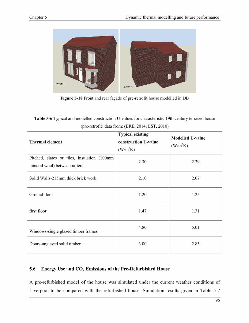
Chapter 5 Dynamic thermal modelling and future performance
95
Figure 5-18 Front and rear façade of pre-retrofit house modelled in DB
Table 5-6 Typical and modelled construction U-values for characteristic 19th century terraced house
(pre-retrofit) data from: (BRE, 2014; EST, 2010)
Thermal element
Typical existing
construction U-value
(W/m2K)
Modelled U-value
(W/m2K)
Pitched, slates or tiles, insulation (100mm
mineral wool) between rafters 2.30 2.39
Solid Walls-215mm thick brick work 2.10 2.07
Ground floor 1.20 1.25
first floor 1.47 1.31
Windows-single glazed timber frames 4.80 5.01
Doors-unglazed solid timber 3.00 2.83
5.6 Energy Use and CO2 Emissions of the Pre-Refurbished House
A pre-refurbished model of the house was simulated under the current weather conditions of
Liverpool to be compared with the refurbished house. Simulation results given in Table 5-7

Chapter 5 Dynamic thermal modelling and future performance
96
shows the annual heating demand, primary energy use and CO2 emissions for the pre- and post-
refurbished houses in Liverpool and significant heating demand reductions of 67% can be seen
after refurbishment. Comparing the CO2 emissions from the house with the average UK CO2
emissions of 5500 kg per person, shows an 85% CO2 reduction after refurbishment; however,
this figure, when compared with the modelled pre-refurbished house, represents a 53% carbon
reduction. One of the reasons of this discrepancy is that kitchen sockets, appliance socket loads
and auxiliary loads cannot be modelled in DesignBuilder and therefore the same assumptions
were made for both pre and post refurbished models.
Table 5-7 Comparison of energy performance and CO2 emissions of pre and post refurbished house for
current Liverpool weather conditions
Predicted parameters Pre-retrofitted Retrofitted
Space heating requirement (kWh/m2.yr) 162 56
Primary energy use (kWh/m2.yr) 291 159
CO2 emissions (kg/m2.yr) 53 25
5.7 Future Performance
5.7.1 Future weather data for simulation
The UK Climate Impacts Programme (UKCIP), in conjunction with the UK’s Meteorological
Office’s Hadley Centre, published its first climate change projections in 1998. These projections
were revised and updated in 2002 and again in 2009 (UKCIP, 2014). In this research climate
change scenarios released by the UK’s Charted Institution of Building Services Engineers
(CIBSE), which incorporated the UKCIP02 projections for three timelines of 2020s, 2050s,
2080s, and four carbon emissions scenarios of low, medium-low, medium-high and high, were
used to generate future hourly weather data for Liverpool (Hacker, et al., 2009). These data were
generated in TRY (Test Reference Year) format but then had to be converted to the EPW
(EnergyPlus Weather) format to be DesignBuilder-readable. CCWeatherGen transforms
CIBSE/Met Office TRY/DSY weather files into current or future EPW weather files. Hence, the
TRY files were morphed in to future weather data using the software CCWeatherGen for three

Chapter 5 Dynamic thermal modelling and future performance
97
time slices: 2020s, 2050s, 2080s; and three carbon emissions scenarios: low, medium and high.
As no TRY files existed for Liverpool at that time, therefore, at the first stages of this research,
future weather files of Manchester were initially used to predict and assess the on-going
performance of the case study. The other problem with using UKCIP02 weather files was the
lack of a probabilistic approach. This gap was then filled in UKCP09 (Hacker, et al., 2009).
Later, Exeter University produced and released EPW future weather files through the
PROMETHEUS project by utilising the UKCP09 weather generator for forty-five locations in
the UK, including Liverpool (University of Exeter, 2011; University of Exeter, 2012). The key
difference between UKCIP02 and UKCP09 was the use of probabilistic information in the latter,
which provided a random sample of a probability distribution function and hence the probability
of a particular level of climate change. Exeter University EPW files were used as the final input
data for this study in order to predict climate change effects on the Liverpool house.
5.7.2 Selecting suitable weather files
With two available emissions scenarios – medium and high; five probabilities – 10, 33, 50, 66
and 90 percentiles; two sets of DSY and TRY files, three timelines – 2030, 2050 and 2080, sixty
sets of future weather files are available for Liverpool. To pick out appropriate weather files for
each step of simulation, comparisons were made between the number of Heating Degree Days
(HDDs) of TRYs and Cooling Degree Days (CDDs) of DSYs for selecting weather files for
heating and cooling requirement estimations respectively. Weather files with maximum,
minimum and near to average number of degree days were selected to estimate the energy
requirements under worst, best and median climate change scenarios; although, when more than
one weather file with the closest number of degree days to the average number was available, the
worst case scenario, based on minimum or maximum external temperatures, was selected for
cooling or heating comparisons respectively.
Figure 5-19 compares annual HDDs of TRY weather files (180C baseline). Based on this graph,
2030 high emissions scenario TRY file with probability level of 10% was considered to estimate
the best case scenario (if fewer changes in heating requirement were to transpire). In terms of
heating requirement, the 2080 high emissions scenario, with a probability level of 90%, was
selected to estimate the worst case scenario. For a central estimate (the median scenario) of the

Chapter 5 Dynamic thermal modelling and future performance
98
possible changes in heating requirement – i.e.– the minimum temperature of three illustrated
options (see Table 5-8) were compared and the 2080 medium emissions scenario TRY file, with
a probability level of 33% with lowest minimum temperature, was selected. However, it is
important to note that, between all available sixty weather files, the 2030 medium emissions
TRY file, with a probability of 10%, had the lowest minimum temperature of -7.3 0C.
Figure 5-19 Annual HDDs of TRY weather file (180C baseline). Data from: (University of Exeter, 2012)
Table 5-8 Minimum temperatures of TRY future weather files for central heating requirement estimate
(the median scenario) Data from: (University of Exeter, 2012)
Emissions and probability 2080 TRY-Med-33 2050 TRY-High-50 2050 TRY-Med-66
Minimum temperature -4.3 -2.3 -3.6
As can be seen in Figure 5-20, the 2080 high emissions DSY weather file with a probability of
90%, has the highest number of CDDs and the 2030 high emissions DSY, with a probability of
2870
2213 2151 2210
1251
0
500
1000
1500
2000
2500
3000
3500
TR
Y-H
igh
-10
TR
Y-M
ed-1
0
TR
Y-H
igh
-33
TR
Y-M
ed-3
3
TR
Y-H
igh
-50
TR
Y-M
ed-5
0
TR
Y-H
igh
-66
TR
Y-M
ed-6
6
TR
Y-H
igh
-90
TR
Y-M
ed-9
0
Num
ber
of
hea
ting d
egre
e d
ays
2030 2050 2080 Average
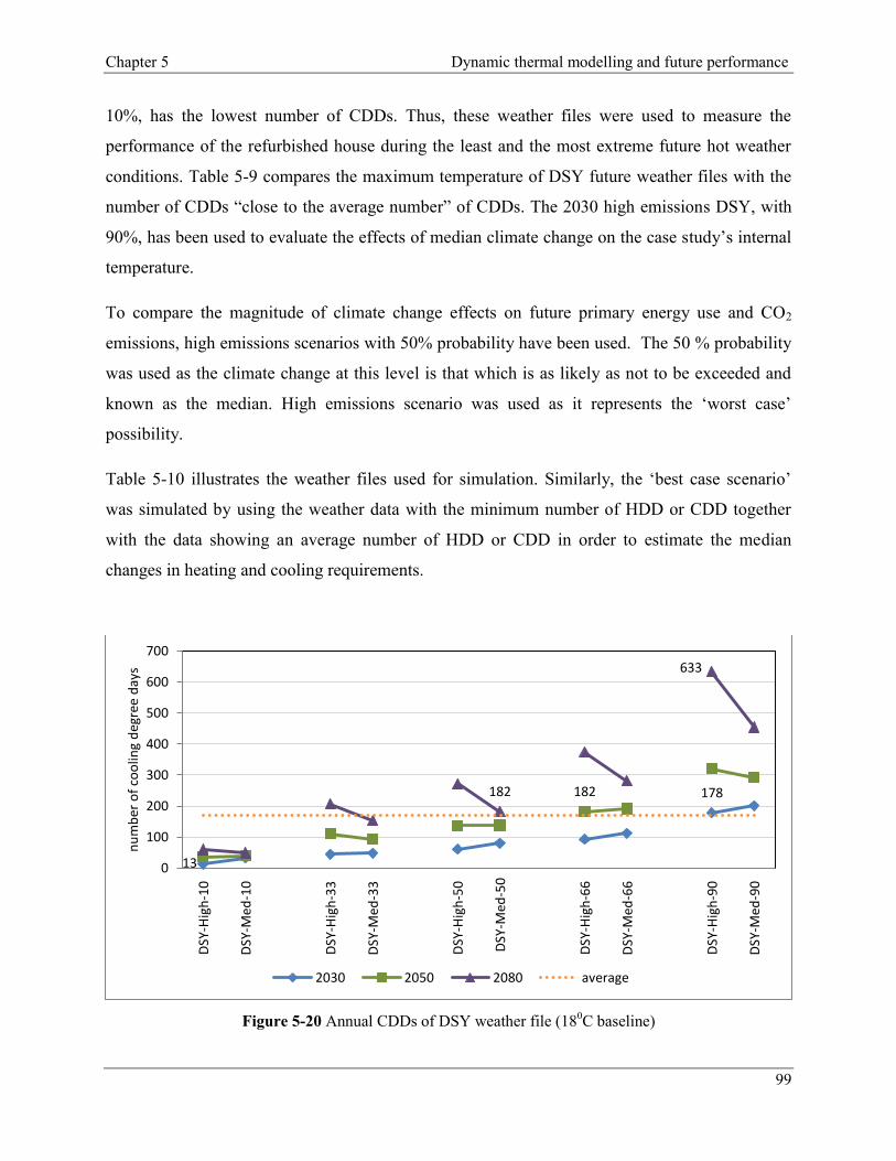
Chapter 5 Dynamic thermal modelling and future performance
99
10%, has the lowest number of CDDs. Thus, these weather files were used to measure the
performance of the refurbished house during the least and the most extreme future hot weather
conditions. Table 5-9 compares the maximum temperature of DSY future weather files with the
number of CDDs “close to the average number” of CDDs. The 2030 high emissions DSY, with
90%, has been used to evaluate the effects of median climate change on the case study’s internal
temperature.
To compare the magnitude of climate change effects on future primary energy use and CO2
emissions, high emissions scenarios with 50% probability have been used. The 50 % probability
was used as the climate change at this level is that which is as likely as not to be exceeded and
known as the median. High emissions scenario was used as it represents the ‘worst case’
possibility.
Table 5-10 illustrates the weather files used for simulation. Similarly, the ‘best case scenario’
was simulated by using the weather data with the minimum number of HDD or CDD together
with the data showing an average number of HDD or CDD in order to estimate the median
changes in heating and cooling requirements.
Figure 5-20 Annual CDDs of DSY weather file (180C baseline)
13
178 182 182
633
0
100
200
300
400
500
600
700
DSY
-Hig
h-1
0
DSY
-Med
-10
DSY
-Hig
h-3
3
DSY
-Med
-33
DSY
-Hig
h-5
0
DSY
-Med
-50
DSY
-Hig
h-6
6
DSY
-Med
-66
DSY
-Hig
h-9
0
DSY
-Med
-90
nu
mb
er o
f co
olin
g d
egre
e d
ays
2030 2050 2080 average

Chapter 5 Dynamic thermal modelling and future performance
100
Table 5-9 Maximum temperatures of DSY future weather files for central heating requirement estimate
(the median scenario) Data from: (University of Exeter, 2012)
Emissions and probability 2080 DSY-Med-50 2050 DSY-High-66 DSY-High-90
Maximum temperature 30.8 30.1 35.1
Table 5-10 The selected weather files used in the simulations
Design scenarios Weather files for simulation
Sensitivity analysis-
Future heating design
Best case 2030 TRY High emissions 10%
Worst case 2080 TRY high emissions 90%
Central estimate 2080 TRY medium emissions 33%
Sensitivity analysis-
Future cooling design
Best case 2030 DSY High emissions 10%
Worst case 2080 DSY High emissions 90%
Central estimate 2030 DSY High emissions 90%
Future performance
2030 TRY High emissions 50%
2050 TRY High emissions 50%
2080 TRY High emissions 50%
5.8 Climate Change Sensitivity Analysis
5.8.1 Space heating energy requirement
The pre and post-refurbished house, viewed under current and future weather conditions and the
various scenarios, were simulated to see the different climate change effects on the heating
requirement. Figure 5-21 shows the results of these simulations. For the best case scenario with
minimum number of HDDs, despite there being no decline in the future heating demand of the
refurbished house, the pre-refurbished house showed an approximate 7% heating demand
reduction due to climate change. Although heating energy consumptions decrease due to climate
change for both refurbished and pre-refurbished houses over the century, a sharp reduction of
more than 65% in energy demand, given all scenarios, happen as a result of eco-refurbishment.
Table 5-11 lists the percentage changes and compares the impact of climate change with
retrofitting based on the heating demand.
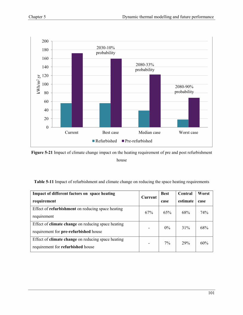
Chapter 5 Dynamic thermal modelling and future performance
101
Figure 5-21 Impact of climate change impact on the heating requirement of pre and post refurbishment
house
Table 5-11 Impact of refurbishment and climate change on reducing the space heating requirements
Impact of different factors on space heating
requirement Current
Best
case
Central
estimate
Worst
case
Effect of refurbishment on reducing space heating
requirement 67% 65% 68% 74%
Effect of climate change on reducing space heating
requirement for pre-refurbished house - 0% 31% 68%
Effect of climate change on reducing space heating
requirement for refurbished house - 7% 29% 60%
2030-10%
probability
2080-33%
probability
2080-90%
probability
0
20
40
60
80
100
120
140
160
180
200
Current Best case Median case Worst case
kW
h/m
2.y
r
Refurbished Pre-refurbished

Chapter 5 Dynamic thermal modelling and future performance
102
5.8.2 Cooling energy requirement
The energy required for cooling the pre and post-refurbished house for different scenarios was
estimated by way of a series of simulations, and the results are illustrated in Figure 5-22. For all
cases and both pre and post-retrofitted house, the energy required for cooling shows a rising
trend. Although cooling demand increased by 80% after refurbishment, very little of the
3.6kWh/m2.yr energy was required for cooling after refurbishment under current, Liverpool,
weather condition. Despite the cooling energy consumptions for the un-refurbished house rose
by 22% under the best case scenario, no increase is shown for future cooling demand for the eco-
refurbished dwelling. Under the worst case scenario, cooling energy use in the pre-refurbished
house is predicted to be more than the cooling energy demand in the refurbished house.
It may be concluded from Figure 5-22 that both refurbished and pre-refurbished houses will
require either a cooling system, or considerable adjustments (or both), in order to maintain
comfortable internal conditions, while Table 5-12 confirms that, over the century, the refurbished
house will show a lower rate of cooling energy increase compared to the non-retrofitted house.
Figure 5-22 Impact of climate change on the cooling energy requirements of pre and post refurbishment
house
Current
2030-10%
probability
2030-90%
probability
2080-90%
probability
0
5
10
15
20
25
30
35
40
Current Best case Median case Worst case
kW
h/m
2.y
r
Refurbished Pre-refurbished
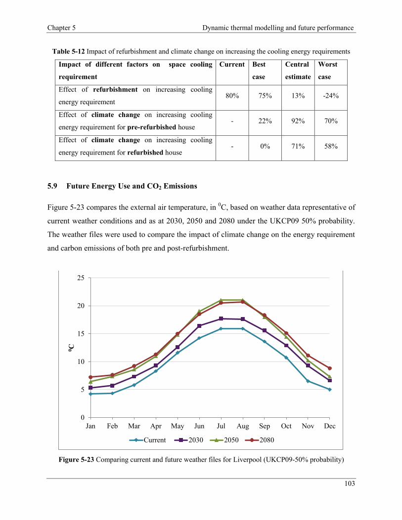
Chapter 5 Dynamic thermal modelling and future performance
103
Table 5-12 Impact of refurbishment and climate change on increasing the cooling energy requirements
Impact of different factors on space cooling
requirement
Current Best
case
Central
estimate
Worst
case
Effect of refurbishment on increasing cooling
energy requirement 80% 75% 13% -24%
Effect of climate change on increasing cooling
energy requirement for pre-refurbished house - 22% 92% 70%
Effect of climate change on increasing cooling
energy requirement for refurbished house - 0% 71% 58%
5.9 Future Energy Use and CO2 Emissions
Figure 5-23 compares the external air temperature, in 0C, based on weather data representative of
current weather conditions and as at 2030, 2050 and 2080 under the UKCP09 50% probability.
The weather files were used to compare the impact of climate change on the energy requirement
and carbon emissions of both pre and post-refurbishment.
Figure 5-23 Comparing current and future weather files for Liverpool (UKCP09-50% probability)
0
5
10
15
20
25
Jan Feb Mar Apr May Jun Jul Aug Sep Oct Nov Dec
0C
Current 2030 2050 2080

Chapter 5 Dynamic thermal modelling and future performance
104
5.9.1 Future heating and cooling energy requirement
The heating consumption results, which appear in Figure 5-24 show that in both cases, heating
energy will decline over the next century. Table 5-13 demonstrates the effect of climate change
on reducing the amount of heating required. The results show that for all scenarios the climate
change impact is always much less than the 65% reduction in heating demand that resulted from
eco-retrofitting.
Figure 5-25 shows the results of a similar study in terms of cooling requirements. In contrast to
heating, this predicts a rising trend over the century for the non-renovated house. For the
refurbished house a rising trend until 2050 can also be seen, but between 2050 and 2080, cooling
energy demand shows a falling trend. Table 5-14 shows that the increase rate for cooling energy
requirement varies for pre and post-refurbished house for different years.
Figure 5-24 Heating energy requirements for current and future weather scenarios
0
20
40
60
80
100
120
140
160
180
Current 2030 2050 2080
kW
h/m
2.y
r
refurbished pre refurbished

Chapter 5 Dynamic thermal modelling and future performance
105
Table 5-13 Effect of climate change on reducing heating energy consumption
Climate change
scenarios-TRY
50% probability
Refurbished
house-Space
heating
requirement
(kWh/m2.yr)
Pre-refurbished
house-Space
heating
requirement
(kWh/m2.yr)
Effect of climate
change on
refurbished
house’s heating
demand
Effect of climate
change on pre-
refurbished
house’s heating
demand
Current 56 162.3 - -
2030 43 136 -23% -16%
2050 35 123 -19% -9%
2080 30 98 -14% -20%
The highest annual rate of cooling energy increase will occur between 2030 and 2050 for the
refurbished house, while, for the pre-refurbished house, the highest increase rate will occur
between 2050 and 2080. This could be due to the fluctuations in the amount of direct normal
solar radiation between 2030 and 2080.
Table 5-15 shows a direct solar radiation increase by 16% between 2030 and 2050. Potentially,
the refurbished house will visibly benefit in terms of cooling by this increase more than the pre-
refurbished house. Likewise, direct solar radiation will decline between 2050 and 2080 by 23%,
and this reflects a falling trend in cooling energy demand between 2050 and 2080 in the
refurbished house.

Chapter 5 Dynamic thermal modelling and future performance
106
Figure 5-25 Cooling energy requirements for current and future weather scenarios
Table 5-14 Effect of climate change on increasing cooling energy consumption
Climate change
scenarios-TRY
50% probability
Refurbished
house-cooling
energy demand
(kWh/m2.yr)
Pre-refurbished
house-cooling
energy demand
(kWh/m2.yr)
Effect of climate
change on
refurbished
house’s cooing
demand
Effect of climate
change on pre
refurbished
house’s cooing
demand
Current 4 1
2030 6 2 50% 100%
2050 16 4 167% 100%
2080 14 13 -12% 225%
Table 5-15 Predicted future direct solar radiation levels
Time Direct Normal Solar
(kWh) Discomfort hours
Percentage of changes in
solar radiation
2030 Jun-Sep 439 123
2050 Jun-Sep 508 106 16%
2080 Jun-Sep 390 219 -23%
0
2
4
6
8
10
12
14
16
18
Current 2030 2050 2080
kW
h/m
2.y
r
refurbished pre refurbished

Chapter 5 Dynamic thermal modelling and future performance
107
5.9.2 Future primary energy use and CO2 emissions
The changes in primary energy use and CO2 emissions from the pre and post refurbished houses
for current and future climates are shown in Figure 5-26 and Figure 5-27 and quantified in Table
5-16 and Table 5-17. According to the figures, primary energy use and consequently CO2
emissions do not show a significant change over the century for either pre- or post-refurbished
houses, although a fluctuation in primary energy demand can be seen in Table 5-16 for the
refurbished house, while a falling trend in its use is shown for the pre-refurbished house between
the current time and 2080.
Figure 5-26 Primary energy use in pre and post refurbished house
Table 5-16 Effect of climate change on primary energy consumption
Climate change
scenarios-TRY
50% probability
Refurbished
house-primary
energy use
(kWh/m2.yr)
Pre-refurbished
house- primary
energy use
(kWh/m2.yr)
Effect of climate
change on
refurbished
house’s primary
energy use
Effect of climate
change on pre
refurbished
house’s primary
energy use
Current 159 291
2030 156 244 -2% -16%
2050 175 237 12% -3%
2080 164 232 -6% -2%
0
50
100
150
200
250
300
350
Current 2030 2050 2080
kW
h/m
2.y
r
refurbished pre refurbished

Chapter 5 Dynamic thermal modelling and future performance
108
Figure 5-27 CO2 emissions from the pre and post refurbished houses for current and future climates
Table 5-17 Effect of refurbishment and climate change on CO2 emissions from the house
Climate change
scenarios-TRY
50% probability
Refurbished
house-CO2
emissions
(kgCO2/m2.yr)
Pre-refurbished
house-CO2
emissions
(kgCO2/m2.yr)
Effect of climate
change on
refurbished
house’s CO2
emissions
Effect of climate
change on pre-
refurbished
house’s CO2
emissions
Current 25 53
2030 26 46 4% -13%
2050 28 45 8% -2%
2080 27 44 -3% -2%
5.10 Summary and Conclusion
The analysis of the future performance of the 19th century terraced house in Liverpool
refurbished to near Passivhaus standards has been divided into two stages, (i) the creation of a
validated model of the pre and post-refurbished houses and (ii) an evaluation of energy
consumption, CO2 emissions and internal thermal comfort, of the houses in the context of future
use. The outcome from the first stage confirms that there can be a significant gap between
0
10
20
30
40
50
60
Current 2030 2050 2080
kg C
O2/m
2.y
r
refurbished pre refurbished

Chapter 5 Dynamic thermal modelling and future performance
109
predicted performance of dwellings – by using computer based building modelling – and actual
performance, and that this mostly originates from failures to factor in occupants’ behaviour,
which is a crucially important factor in the performance of particularly low energy dwellings.
Although, long-term monitoring will help to improve estimates of the actual energy end-use
breakdown in order to realise the baselines for different types of buildings and their occupancy, it
is still possible to validate the computer models to an acceptable level by utilising available
energy bills, semi-structured or structured interviews and by comparing the model technical
input data to standards. Additionally, special care must be taken in detailing the identifiable
parameters.
Results from the second stage indicate that energy demands and CO2 emissions experienced a
sharp decline following eco-refurbishment. simulating the building under different probabilities
shows that a full probabilistic prediction of thermal building performance on a time scale of 50-
80 years is likely to be accompanied by large uncertainties; however, in all the types of cases
reviewed, the need to minimize over-heating, together with the maintenance of acceptable
internal temperatures, will become increasingly important factors in design decision making.
The life expectancy of most buildings’ services is much shorter than that of the buildings
themselves, which means that service systems are likely to need replacing after between fifteen
to twenty years; hence, climate change effects on such a short time scale will be marginal, which
will give plenty of opportunity to install new systems that can cope with changing conditions.
Therefore, back-up systems that provide for additional heating and cooling capacities should be
considered as safety factors
There is a scope to retrofit millions of buildings in order to make deep cuts in CO2 emissions, but
this is clearly both a major environmental and economic task. It is therefore crucially important
that carbon cuts can be achieved at the expenses of other factors, such as monetary payback time.
Consequently, the next chapter will consider life cycle economic assessment and environmental
life cycle assessment for the whole house refurbishment.

Chapter 6 – Life Cycle Assessment of Eco-Refurbishment
6 Not erase Not erase

Chapter 6 Life cycle assessment of eco-refurbishment
111
6.1 Chapter Overview
Studying the current and projected future energy performance of the retrofitted house in Liverpool
revealed that an eco-retrofit was a relatively effective route to energy and carbon emissions savings
during the operational stage. However, since a refitted building will function for many more years, a
life cycle cost and carbon emissions assessment should be accounted in such a way so as to make sure
that energy and carbon cuts are achieved at the expense of other factors, such as monetary and carbon
payback times. Therefore, the life cycle economic assessment and environmental life cycle assessment
for the whole house refurbishment will be presented in this chapter. However, previous chapters have
uncovered a number of uncertainties in predicting the future energy performance of the refurbished
house. In addition, evaluating the lifetime carbon and cost of its performance in this chapter revealed
that the results are also sensitive to (i) the assumed lifespan of the building measures, and (ii) the cost
of fuel and (iii) discount rates. Hence, the effect of possible variations in these values has been
considered on lifetime carbon and costs analysis.
It has been made clear in previous chapters that there are economic and practical grounds to retrofit
millions of houses in order to make deep cuts in CO2 emissions which, it is acknowledged, would be a
huge task. Therefore, it has been useful to assess the carbon and cost efficiency of individual retrofit
measures such as building fabric, window refitting, building services and renewables. This has been
done by using a combined life cycle cost and carbon analysis and by comparing the efficiency of each
individual measure based on the cost of each item against one tonne of carbon saved.
The analysis shows that the carbon payback time is shorter than the financial payback for the eco-
refurbishment of the whole house. The whole house refurbishment’s initial cost will be paid back in
less than fifty years, taking into account upward gas price trends, while the carbon payback time of
whole efficient measures is less than seven years.
6.2 Introduction and Objectives
In deciding whether to refurbish or demolish a building, the key factors, are, (i) embodied carbon, and
(ii) cost of refurbishment. Both of these factors, especially the embodied carbon of refurbishment, are
often overlooked in ‘rebuilt or refit’ arguments. Kemp and Wexler estimated the embodied carbon of a
new home at thirty-five tonnes of CO2 (CAT, 2010). Constructing the Camden Passivhaus in London
cost £4455/m2
– see chapter 3, section 3.5.6 – (Ridley, et al., 2013), while the Liverpool house’s
whole renovation and refurbishment to near Passivhaus standard cost £2168/m2 with only £687/m
2 of

Chapter 6 Life cycle assessment of eco-refurbishment
112
this spent on energy efficiency measures. However, Decisions over the cost effectiveness of
refurbishment should really be made by comparing initial costs with cumulative savings over the
building’s life – between fifty and a hundred years – and the payback time of refurbishment compared
to new build. Table 6-1 compares the initial cost and first year carbon emissions for the Liverpool
refurbished house and the new build Camden house. The same comparison is required for carbon
reduction studies.
In the UK the focus of legislation is on reducing carbon emissions and energy use in the operational
stage of a building, including the CO2 emissions from energy consumption due to lighting, heating and
ventilation. Hence, using new and improved technologies in more buildings has increasingly improved
building energy efficiency and reduced carbon emissions created in the operational stage (DCLG,
2007). This improvement is often achieved by more energy demand and consequently carbon
emissions in the material production stage (the embodied carbon), which explains the growing
importance of the non-operational energy consumed and carbon emitted; thus, during other stages in a
projects’ life cycle, such as the carbon emissions created in the manufacture of the materials,
transportation, construction activities and the eventual demolition and disposal, can be very costly
(Gustavsson, Joelsson and Sathre, 2010; Sahagun and Moncaster, 2012). Therefore, a second objective
of this chapter is to estimate the carbon payback times of the retrofit to establish how savings in CO2
emissions might relate to the operational carbon emissions during a building’s life cycle. Two different
methods are used to assess the life time cost and carbon footprint of refurbishment and it is important
not to confuse them; however, both methods should be considered whenever environmental impacts
are a concern.
It is also important to establish which individual retrofit measure, such as insulation or glazing, results
in the greatest overall reduction in the carbon emissions and energy cost in the long term. This will
help decision makers to recognise how to balance the competing objectives of cost and energy.
Therefore, this chapter also uses Sweetnam and Croxford’s (2011) method for weighting energy
efficient refurbishment measures used for the refurbishment of the Liverpool house. (sweetnam and
Croxford, 2011).
The validated model of the pre and post refurbished house, as outlined in the previous chapter, was
used as the base for simulating the effects of eco-refurbishment on savings in costs and CO2 emissions
from gas usage for water and space heating. Computer-generated carbon and energy savings were then
applied as inputs to obtain a cost and carbon life cycle assessment model. Also, energy efficient

Chapter 6 Life cycle assessment of eco-refurbishment
113
measures were added to the pre-refurbished house one by one to demonstrate how each measure might
affect savings.
Table 6-1 Comparison of the initial cost and first year carbon emissions for the Liverpool refurbished house and
the new build Camden house.
Project Initial cost of project (£) Annual CO2 emissions after
monitoring (kgCO2/m2)
Broxton street house, Liverpool £193,308 (£61,260 for energy
efficiency measures) 23.6
Camden house, London £450,000 24.3
6.3 Methods, Definitions and Scope of Analysis
6.3.1 Life cycle carbon emissions
With more energy efficient measures coming to the construction industry, the relative importance of
CO2 emissions from buildings has shifted from operational emissions to energy consumed, which will
affect carbon emissions during other project life cycle stages. These include:
1. Extraction and manufacturing stage – cradle-to-gate carbon emissions:
Mining, raw material extraction, processing and manufacturing stage
2. Transportation stage – cradle-to-site carbon emissions:
Emissions from the cradle-to-gate stage, plus delivery to the construction/installation site
3. Assembly stage – cradle to end of construction:
Sum of cradle-to-site, construction and assembly on site stage
4. Replacement, or deconstruction, stage – cradle-to-grave carbon emissions:
Emissions from cradle to end of construction plus maintenance, refurbishment, demolition,
waste treatment and disposal stage:
5. Cradle-to-cradle – or recycling the material stage

Chapter 6 Life cycle assessment of eco-refurbishment
114
The life cycle carbon footprint is the cradle-to-gate carbon emissions, minus carbon saved as a result of
energy savings during refurbishment. Equation 6-1 can be used to calculate the life cycle carbon
footprint of a building (RICS, 2012; Bull, et al., 2014).
𝐿𝐶𝐶𝐹 = ∑(𝐸𝐶𝑚𝑖
𝑁𝑖
𝑖=0
+ (∑ 𝑇𝐶𝑡
𝑁𝑡
𝑡=0
𝑚𝑖𝑘𝑚𝑖) + 𝑊𝐶𝑚𝑖 − 𝑅𝐶𝑚𝑖) − ∑ 𝐹𝑆𝐶𝑦
𝑁𝑦
𝑦=0
Equation 6-1
where
LCCF = marginal life cycle carbon footprint
Ni = number of materials i
mi = marginal mass of material i in tonnes
Nt = number of transport modes t
kmt = total distance transported by mode t in km
EC = embodied carbon of material i in tonneCO2e/tonne
TCt = transport carbon of transport mode t in tonneCO2e/tonne km
WCi = waste carbon of material i in tonneCO2e/tonne
RCi = carbon credit for recycling of material i in tonneCO2e/tonne
Ny = number of years in the time horizon
FSCy = carbon credit of fuel saved in year y in tonneCO2e
6.3.1.1 Scope of the analysis
To determine the carbon costs and carbon payback time of improving construction in the Liverpool
eco-refurbished case study the cradle-to-site carbon emissions of the renovation were calculated. Other
stages have been discounted as (i) research by HM Government (2010) has shown that after the
operational stage, the manufacturing stage is the second most significant area of carbon emissions from
the entire life cycle of a building, and (ii) the case studies suggest that the contribution of other stages
to carbon footprint is lower than 10% of carbon emissions from the entire life cycle of a building and

Chapter 6 Life cycle assessment of eco-refurbishment
115
(iii) Kellenberger and Althaus (2009) suggests that input of lower than 10% would not have a major
impact on the result of analysis; (HM Government, 2010; Kellenberger and Althaus, 2009; Sahagun
and Moncaster, 2012). Therefore, Equation 6-2 was used to estimate LCCF of the retrofit to discover
how savings in CO2 emissions might relate to the operational carbon emissions during the building’s
life cycle when compared with the non-refurbished house.
𝐿𝐶𝐶𝐹 = ∑ 𝐸𝐶𝑚𝑖
𝑁𝑖
𝑖=0
+ (∑ 𝑇𝐶𝑡
𝑁𝑡
𝑡=0
𝑚𝑖𝑘𝑚𝑖) − ∑ 𝐹𝑆𝐶𝑦
𝑁𝑦
𝑦=0
Equation 6-2
6.3.1.2 Data for analysis and assumptions
Embodied carbon and marginal mass of materials (tonnes)
The Inventory of Carbon and Energy (ICE) database from Hammond and Jones (2011) at the
University of Bath was selected as a database to calculate the embodied carbon of fabric measures,
glazing and doors and the results added together to calculate the embodied carbon. (Hammond and
Jones, 2011). The suggested quantity conversion factors from the same source were used to calculate
marginal mass of materials in tonnes using Equation 6-3. A petrol carrying vehicle is considered to be
the mode of transport for all materials (see Chapter 4 for more information about the materials).
Quantity (tonnes) = m3× Unit Conversion or Density (tonnes/m
3) Equation 6-3
The procedure for calculating embodied carbon of services and solar thermal panels, however, was
more complicated. Kalogirou 2004 has calculated the embodied energy of a 1.9m2 flat plate collector
which, together with process energy, resulted in an overall embodied energy value of 3,540 MJ per
module, with a total embodied energy value for a 2-panel installation amounting to 8,700 MJ,
equivalent to 2417 kWh and 0.47 tCO2e . In this study other components, such as hot water cylinders,
insulation and pumps, were discounted from analysis since similar systems would be present in any
existing house (Kalogirou, 2004). Another study by Bull, et al., (2014) considered 0.85 tCO2e as a
suitable equivalent for these services. Transportation from Germany has been considered for the
MVHR and boiler, but because the systems are now available in the UK, the replacement
transportation amount will only make a small impact. (Bull, et al., 2014).

Chapter 6 Life cycle assessment of eco-refurbishment
116
Carbon saved during operational stage
Only gas consumption and carbon saved from water heating and space heating, due to adding energy
efficient measures to the Victorian house, have been included in this analysis. These data have been
arrived at from both modelling and simulation of the pre-refurbished house and actual monitoring data
from the refurbished house. The carbon saved during the operational stage has been calculated using
Equation 6-4.
Carbon saved (tCO2) = Operational CO2e (existing house – refurbished house ) Equation 6-4
6.3.2 Carbon payback time of eco-refurbishment
One of the key aims of this chapter was to estimate the carbon payback time of the eco-refurbishment.
The cumulative embodied carbon of refurbishment was therefore compared with the expected changes
– i.e. savings in the carbon emissions of the existing house, pre-refurbishment, as a result of the
retrofit.
6.3.3 Whole life-cycle costing
Whilst fulfilling an 80% reduction goal and meeting eco-refurbishment benchmarks, one of the most
important questions was that of economic feasibility. This arises because of several potential
alternative investment options and the importance of finding the most economical long-term choice. In
this chapter, a Whole Life Cycle Costing (WLCC) technique has been used for comparative cost
assessments over seventy years, taking into account the present value of initial capital costs, future
operational costs and savings from this type of eco-refurbishment.
6.3.3.1 Scope of WLCC
WLCC considers the total expense of a project over six stages of: (i) non-construction, (ii)
construction, (iii) operations, including energy expenditures, (iv) maintenance, (v) replacement, and
(vi) disposal. For the purpose of this research, the effects and savings on gas consumption for space
and water heating from improving design, construction and the HVAC system have been evaluated.
The WLCC of fitting ground floor, wall and roof insulation, replacing windows, doors, boiler and also
low and zero solar thermal carbon technologies, have been assessed. However, the costs and effect of

Chapter 6 Life cycle assessment of eco-refurbishment
117
improvement, replacements and disposal have not been considered due to a lack of information about
the products in the supply chain. Transportation costs are also ignored for the WLCC analysis. Table
6-2 shows the scope of the WLCC study. Equation 6-5 shows that the Whole Life Cycle Cost is
defined as (Task Group 4, 2003):
𝑊𝐿𝐶𝐶 = 𝐼𝐶 + ∑𝑂𝐶𝑡
(1 + 𝑟)𝑡
𝑁
𝑡=1
Equation 6-5
where:
WLCC = Whole Life Cycle Cost (£),
IC = Total Initial Cost (£),
∑= Sum over the lifetime, from year 1 to year N, where N = lifetime of appliance (years),
OCt = Operating Cost (£),
r = Discount rate,
t = Year for which operating cost is being determined
Table 6-2 Scope of WLCC study
Stage Covered in WLCC
Non-Construction Costs Costs of material, services and renewable technologies
Construction Costs Costs of labour and installation
Operation Costs Costs of space and water heating energy consumption (gas)
Maintenance Costs -
Replacement Costs -
Disposal Costs -

Chapter 6 Life cycle assessment of eco-refurbishment
118
6.3.3.2 Maintenance and repair costs
Refurbished house
In this study it is assumed that the life of the construction in this refurbished property will be more than
fifty years. For the Liverpool house, the system selected and installed is a Paul Novus 300 whole-
house mechanical ventilation with heat recovery (MVHR) system which, according to the company,
has a lifespan equal to the building’s life time. Any recurring impacts, such as repairs and maintenance
costs, are not considered here, since the building was refurbished in such a way as to have very low
maintenance costs. However, as Sodagar, et al. (2009) state, maintenance costs of a pre-refit building
can contribute significantly to the total cost analysis (Sodagar, et al., 2009).
Pre-refurbished house
For the pre-retrofitted house the basic maintenance and repair costs of the pre-refit building has been
added to the operational costs. The English Housing Survey, Housing stock report 2012 has defined
basic repairs as any urgent repairs plus additional visible work to be carried out in the medium term
(within five years). These do not include replacement of building elements nearing the end of their life
where the surveyor has recorded that this action could be delayed by more than five years (DCLG,
2012).A figure of £14/m2 has been suggested for basic repair (day to day maintenance). This measure
is compatible with a suggested basic repair costs of a Victorian end terraced house by Southampton
City Council (Southampton city council, 2014). A private sector housing condition survey has been
used in this study to suggest the repair costs (Opinion Research Services, 2012). Table 6-3 shows the
required repairs and frequency of that during 60 years of building life. As these repairs will be done in
the future, a discount rate has been considered when adding them to the operational cost of pre-
refurbished house (see section 6.3.3.4 for more details on discount rate).
Table 6-3 Repair costs of a 130 year old pre-refurbished house during 60 years of building lifetime: data from
(Southampton city council, 2014)
Item/frequency 1th years only Every 2 years Every 3 years Every 20 years
Roofs - £303
Ceilings - £253
External walls, windows and doors 12981 £505
Internal walls and doors - £150
Boiler - £2000

Chapter 6 Life cycle assessment of eco-refurbishment
119
6.3.3.3 Total initial costs inputs (IC)
The cost for energy efficiency measures (fabric insulation, replacing doors and windows, low carbon
technologies, and building services) in this project totalled £61,260. The cost breakdown of the energy
efficient measure of the study house can be seen in Table 6-4.
Table 6-4 Cost breakdown for the terraced house’s refurbishment
Item
Construction Phase Comments
Material Labour
Fabric measures £12,000 £7,000
Building services £9,050 £2,500 MVHR and boiler
Low/zero carbon technologies £6,560
Solar Thermal
Renew roof £1,950 £2,000
Triple glazing and doors £18,200 £2,000
6.3.3.4 Operating cost inputs
The processes during the in-use life phase are important factors, since a significant proportion of the
impact of the building occurs after the construction and installation of systems. Required input for
calculating operating costs is annual cost savings results from energy savings which is sensitive to the
effect of (i) climate change (ii) gas prices (£) and (iii) assumed discount rates.
(i) The effect of climate change on annual savings
Climate change will impact on heating consumption in the pre and post-refurbished house.
Accordingly, different climate change scenarios have been considered and predicted by running
simulations for the best, median and worst case scenarios in order to evaluate the savings from the
existing and refurbished house.
(ii) The effect of Gas energy savings on annual savings
The total annual gas saving is the difference between the heating consumption of the original house
and the retrofitted house, as a result of the lower gas heating consumption arising from a more efficient

Chapter 6 Life cycle assessment of eco-refurbishment
120
construction and lower heat losses due to insulation, triple-glazed windows and the new boiler and
solar thermal for DHW.
Figure 6-1 compares gas price projections from eight different sources (Bolton, 2008). Experts in
energy economics believe that the main question about future gas prices is not ‘will prices rise?’ but
‘by how much?’ While historic data of the UK gas prices for forty years since 1970, shown in Figure
6-2, reveals how the price of gas has been unstable (Friends of the Earth, 2012). The UK government’s
energy regulator, The Office of Gas and Electricity Markets (Ofgem), estimated contributory factors to
domestic energy price rise can be seen in Table 6-5. However, other factors such as (i) any policy to
lower dependency on imports, (ii) greater domestic production and (iii) the pace at which technology
increases would result in falling gas prices. For instance, in the USA a rapid revolution in gas
production from ‘unconventional’ sources – in particular shale and coal bed gas – has transformed the
market, to the extent that it is now self-sufficient in gas. Some analysts predict that this could
eventually happen in the UK (Friends of the Earth, 2012). Hence, there is uncertainty in assuming or
future gas prices and in real terms energy prices will not remain constant over time.
Figure 6-1 DECC gas price projections, October 2011 (Bolton, 2008)

Chapter 6 Life cycle assessment of eco-refurbishment
121
Table 6-5 Estimated contributory factors to domestic energy price rise Feb 2004 to Jan 2011 (Friends of the
Earth, 2012)
Increase in unit costs due to: %
Whole sale energy 66
Transmission, distribution and metering 20
Carbon price -
Renewables -
Energy efficiency funding 7
VAT 5
Overall price increase 121
Estimated increase in annual bill (2004 to 2010) £295
However, by using historic data, it is possible to predict the range of probable future prices and to have
some idea of when price changes are more likely to occur (Ellingham and Fawcett, 2006).
Consequently, both lifetime cost performance and cost payback time of the case study have been
estimated for all possible ‘waves’ of rising, falling and steadying domestic gas prices trends.
Figure 6-2 Energy prices (pence/kWh) since 1970 (Friends of the Earth, 2012)
0.0
0.5
1.0
1.5
2.0
2.5
3.0
3.5
4.0
4.5
5.0
1970 1975 1980 1985 1990 1995 2000 2005 2010
p/k
Wh

Chapter 6 Life cycle assessment of eco-refurbishment
122
Standard deviation and binomial tree
The degree of uncertainty in the future price of a commodity such as gas can be calculated by drawing
a binomial tree. In this study 41 years of gas price (1970-2011) datasets were used to adjust the
projection of future uncertainty, predict future gas prices and find the future outcomes. The instability
of a data series is measured by its standard deviation (S), which can be used to indicate the rising and
falling values by means of a binomial tree –see Figure 6-3 (Ellingham and Fawcett, 2006).
Figure 6-3 Binomial Tree
Drawing a binomial tree helps to predict the expected future gas prices and related savings. The
expected value (steady gas prices) in each year is the average of all possible outcomes, weighted by
their probability. However, for upward and falling gas scenarios only the scenarios with more than 1%
probability have been considered as a predicted upward gas price of each year and upward trend has
been presented as favourable upward trend.
(iii) Time preference, discount rate and net present value
The discount rate ‘r’, which is the rate at which future expenditures will be discounted to establish
their present value, is defined as the value society attaches to present, as opposed to future,

Chapter 6 Life cycle assessment of eco-refurbishment
123
consumption (Hanton, 2010). This rate is required to enable the costs of paying future liabilities to be
put into present-day terms – a parameter called ‘the net present value’ (NPV) (Ellingham and Fawcett,
2006). A discount rate of 3.5% has been chosen as this is used by the Government for economic
decision making. Please note that inflation has not been taken into account in this research (HM
Treasury, 2011). Applying this 3.5% discount rate to the savings enables the NPV of the savings to be
calculated. If all the expenditures and incomes in a cash flow (v0, v1, v2,…,vn) are discounted to their
present values using the chosen discount rate and then aggregated, the result is the net present value of
the cash flow (see Equation 6-6) (Ellingham and Fawcett, 2006).
𝑁𝑃𝑉 = 𝑣0 +𝑣1
(1 + 𝑟)+
𝑣2
(1 + 𝑟)2+ ⋯
𝑣𝑛
(1 + 𝑟)𝑛 Equation 6-6
6.3.4 Monetary payback period
The payback period is calculated by deducting the fuel cost saved each year from the capital cost of the
energy saving measures. To assess the time required to recover the initial costs of eco-refurbishment
with constant, growing and decreasing energy prices, the amount of corresponding discounted saving
costs were added to the initial annual cost of efficiency measures and the cumulative cash flow of the
refurbished house, given the various trends, was compared to the cumulative cash flow of the pre-
refurbished house.
6.3.5 Methodology for comparing the cost of each tonne of carbon saved (CTS) for individual
energy efficient measures
When examining a low energy building, a whole-house approach is necessary since, when the overall
energy use decreases, the interaction between energy efficiency measures becomes more important and
so the house should be seen as a whole. Thus, methodologies used for a whole-house, life-time cost
and carbon performance analysis were described in the previous sections. On the one hand, energy and
carbon reductions in the Liverpool house were achieved by incurring high cost expenses; however,
there are millions of houses in the UK which require this level of refurbishment to meet the 80%
reduction target. On the other hand, a wide variety of owner and refurbishment drivers, such as
government, social landlords, housing associations and local authorities, will be involved. Therefore,
in order to encourage the refurbishment practice, it will be necessary to tailor the most effective

Chapter 6 Life cycle assessment of eco-refurbishment
124
options required to reduce carbon emissions for each home owner and stakeholder. It is essential to be
able to demonstrate how well the various technologies are likely to work.
In order to achieve this, a cost analysis of individual measures will help to establish the contribution of
each measure to carbon saving and its initial cost. This information will also help decision makers to
recognise how to balance the competing elements of cost and energy. Sweetnam and Croxford’s cost
per tonne of carbon saved (CTS) methodology, which combines the lifetime cost saving assessment
method with the carbon footprint assessment method, has been used in this study for each energy
efficient measure. In this calculation the effect of climate change and fluctuations in gas prices are
discounted, since the aim is to achieve a comparative analysis rather than a confirmatory analysis – see
Equations 6.7 and 6.8 (sweetnam and Croxford, 2011).
𝑪𝒂𝒓𝒃𝒐𝒏 𝒔𝒂𝒗𝒆𝒅 (𝒕𝑪𝑶𝟐) = [(𝑶𝑪 𝒆𝒙𝒊𝒔𝒕𝒊𝒏𝒈 𝒉𝒐𝒖𝒔𝒆 − 𝑶𝑪 𝒓𝒆𝒇𝒖𝒓𝒃𝒊𝒔𝒉𝒆𝒅 𝒉𝒐𝒖𝒔𝒆) x Lifespan] - £EC Equation 6-7
𝑪𝑻𝑺 (£ 𝒕𝑪𝑶𝟐⁄ ) = 𝐂𝐚𝐫𝐛𝐨𝐧 𝐬𝐚𝐯𝐞𝐝
𝐖𝐋𝐂𝐂 Equation 6-8
where CTS is cost per tonnes of carbon saved.
6.4 Results and Discussion
6.4.1 Embodied carbon of materials used in the Liverpool end-terraced house
Table 6-6 demonstrates the breakdown of embodied carbon for all of the energy efficiency measures.
A comparison between cradle-to-gate carbon emissions of materials with the embodied carbon in
transportation activities shows that most of the embodied carbon is created at the manufacturing stage.
Figure 6-4 demonstrates that external wall insulation has the highest embodied load of embodied
carbon, with 4.94 tonnes, whereas roof and floor insulation have the lowest embodied burdens with
0.35 tCO2e.

Chapter 6 Life cycle assessment of eco-refurbishment
125
Table 6-6 Cradle-to-site embodied carbon (EC) of efficient measures for refurbishment
Energy efficient
refurbishment measure
Cradle-to-gate EC
tCO2e
EC of transportation
tCO2e
Cradle-to-site EC
tCO2e
External wall insulation 4.74 0.01 4.94
Ground floor insulation 2.04 same as external wall 2.04
Windows 1.34 0.58 1.92
Internal partitions 1.85 same as external wall 1.85
Roof and floor insulation 0.34 0.01 0.35
Solar thermal and Services 1.70 0.01 1.72
Doors 1.02 0.58 1.60
Services 0.85 0.09 0.94
Cradle-to-site embodied carbon of efficient measures for refurbishment 15.36
Figure 6-4 Cradle-to-site embodied carbon of efficient measures for refurbishment
4.94
2.04 1.92 1.85 1.72 1.60
0.94
0.35
0
1
2
3
4
5
6
Exte
rnal
wal
l in
sula
tion
Gro
und f
loor
insu
lati
on
Win
dow
s
Inte
rnal
par
titi
ons
Sola
r th
erm
al a
nd S
erv
ices
Doors
Ser
vic
es
Roof
and f
loor
insu
lati
on
tCO
2e

Chapter 6 Life cycle assessment of eco-refurbishment
126
6.4.2 Life-cycle carbon emissions and carbon payback time of eco-refurbishment
Figure 6-5 compares the carbon emissions from gas consumption for water and space heating energy
before and after applying energy efficient measures to the Victorian house. The refurbishment process
saved 2.03 tonnes of CO2e. The figures in Table 6-7, along with embodied carbon of refurbishment
were used to estimate the carbon payback time of eco-refurbishment. Table 6-8 presents the
cumulative carbon emissions of the pre- and post-refit house from space heating gas energy
consumption.
Figure 6-5 indicates that, between the seventh and eighth year, the carbon costs incurred in improving
the construction and replacing all windows and doors, installing the solar thermal system and other
new services, have been recovered. Consequently, the embodied carbon can be considered to be a good
carbon investment. Year 0 represents the year of the refurbishment and the point on the y-axis shows
the amount of embodied CO2e. The angle at which the lines inclines depends on the amount of annual
operational carbon and the point at which they intersect represents the payback period, i.e. the point at
which the additional carbon costs arising from the retrofit have been recovered.
Table 6-7 Emissions from gas usage for space heating and DHW energy consumption (tonnes CO2/yr)
Item measured Pre-Refurbished Refurbished
Operational carbon emissions
(tonnesCO2/yr) 3.08 1.05
Figure 6-5 Carbon payback time of refurbishment
0
5
10
15
20
25
30
35
0 1 2 3 4 5 6 7 8 9 10
tCO
2e
Years
Refurbished house Pre-refurbished house

Chapter 6 Life cycle assessment of eco-refurbishment
127
Table 6-8 Cumulative carbon emissions of pre and post refit house from gas usage for water space heating
energy consumption (tonnes CO2/yr)
Years 0 1 2 3 4 5 6 7 8
Refurbished house 15.0 16.05 17.10 18.15 19.2 20.25 21.3 22.35 23.40
Pre-refurbished house 0 3.08 6.16 9.24 12.32 15.40 18.48 21.56 24.64
6.4.3 Whole life cycle cost assessment results
6.4.3.1 Effect of climate change on annual savings
One of the parameters required for WLCC assessment is the operational cost before and after
refurbishment. However, this factor is subject to change due to uncertainties regarding the weather
conditions under which the house is being simulated. Therefore, the effect of climate change on annual
savings has been taken into consideration in this section. Pre and post-refurbished houses under current
and various – i.e. best, median and worst – future weather scenarios were simulated to estimate the gas
consumption reduction that would be achievable as a result of refurbishment (see Figure 6-6 for
simulation results). The graph depicts how energy consumption – i.e. savings – differs depending on
the various climatic scenarios. See Table 6-9 for comparisons of savings for different climatic
scenarios).
Figure 6-6 Annual space and water heating demand for the pre and post-refurbished terraced house under
different climate scenarios
0
2000
4000
6000
8000
10000
12000
14000
16000
18000
Curr
ent
2030-
bes
t
2050-
bes
t
2080-
bes
t
2030-
med
ian
2050-
med
ian
2080-
med
ian
2030-
wors
t
2050-
wors
t
2080-
wors
t
kW
h/y
r
pre-refit post-refit

Chapter 6 Life cycle assessment of eco-refurbishment
128
Table 6-9 Effect of climate change on gas energy savings after refurbishment (kWh)
Climate change scenarios Gas energy savings after
refurbishment (kWh)
Current 10007
2030- best case scenario 9216
2050- best case scenario 8975
2080- best case scenario 8564
2030- median case scenario 7969
2050- median case scenario 7594
2080- median case scenario 7053
2030- worst case scenario 7257
2050- worst case scenario 6476
2080- worst case scenario 4951
6.4.3.2 Effect of future gas prices uncertainty on annual savings
The energy savings cost is the difference between the cost of gas bills of the pre-refit and the retrofit
house. Because gas is the primary energy source for space and water heating in this case study, the
energy cost is calculated by using a mean gas price of 5.29p/kWh. The annual benefit – i.e. the
financial saving – is calculated by multiplying the energy saving by the current gas price of 5.29p/kWh
for the first year of the cash flow (see Table 6-10 for the numerical result for the current weather data).
Table 6-10 Annual savings from lower gas consumption for water and space heating – current weather data
Climate
scenarios
Estimated annual
gas bill for existing
house (£)
Estimated
annual gas bill
for refurbished
house (£)
Annual
energy (gas)
cost savings
(£)
Liverpool –
Current
weather
£828 £299 £529

Chapter 6 Life cycle assessment of eco-refurbishment
129
Future gas prices
Because cost benefit analyses are performed over the lifetime of a house, a changing rate has to be
introduced if the cost calculations are to correspond with reality. The historical data suggests that not
only will energy prices fluctuate there is also a possibility of both downward and upward trends;
hence, different scenarios should be investigated that take these into account. To measure the amount
of uncertainty, and to predict gas price trends, forty years of gas price datasets were used and the
change over time – i.e. the standard deviation – was calculated, using, which resulted in an annual
variation instability of 8.9% (see Table 6-11 and Equation 6-9). As a consequence, this ratio, which
effectively allows for rising and falling gas prices over the next fifty years, a binomial tree of price
trends can be constructed.
Figure 6-7 illustrates the predicted different possible gas prices for each year. The expected gas price is
the sum of all possibilities, weighted by their probabilities. For a better comparison, a different scale
has been chosen on the right vertical axis, which shows the predicted prices for a favourable upward
trend, while the left vertical axis illustrates the projected gas prices for (i) a constant and (ii) falling
trend and also (iii) rising trends in gas prices with a probability of more 1%.
Table 6-11 Average annual standard credit bills (£) for a typical residential gas consumer for 16 years since
1996 source (Friends of the Earth, 2012)
Years Gas prices (pence/kWh) Annual % variation Instability
1970 4.58 - -
1971 4.22 -7.9 -8
1972 4.05 -4 -4.2
1973 3.66 -9.6 -9.8
1974 3.19 -12.8 -13
1975
.
.
.
2008
2.93
.
.
.
3.66
-8.2
.
.
.
14.4
-8.3
.
.
.
14.2
2009 4.16 13.7 13.5
2010 3.84 -7.7 -7.9
2011 4.19 9.1 9
Average of change 0.16

Chapter 6 Life cycle assessment of eco-refurbishment
130
𝑠𝑡𝑎𝑛𝑑𝑎𝑟𝑑 𝑑𝑒𝑣𝑖𝑎𝑡𝑖𝑜𝑛 (𝑠) = √(−8)2 + (−4.2)2 + (−9.8)2 + ⋯ (9)2
(42 − 1)= 8.9 Equation 6-9
Figure 6-7 Predicted possible prices for gas
6.4.3.3 Discounted cash flow and future energy saving cost
By estimating future gas prices and predicting future energy requirements, it is possible to calculate the
building’s energy expenditure savings which, because different operations take place at different times,
have to be converted to current costs by using a discounted cash flow method using Equation 6-6 that
incorporates the discount rate of 3.5% for the first thirty years and 3% thereafter. see Table 6-12 for
the values for Liverpool for 2010 to 2030.
0
50
100
150
200
250
300
350
0
5
10
15
20
25
Curr
ent
20
12
20
14
20
16
20
18
20
30
2022
20
24
20
26
20
28
20
30
20
32
2034
20
36
20
38
20
40
20
42
20
44
2046
20
48
20
50
20
52
20
54
20
56
2058
Fav
ou
rab
le u
pw
ard
tre
nd
(p
/kW
h)
pro
bab
le c
onst
ant,
risi
ng
an
d f
alli
ng
pri
ces
(p/k
Wh
)
Probable upward trend Constant trend
Probable falling trend Favourable upward trend

Chapter 6 Life cycle assessment of eco-refurbishment
131
Table 6-12 Future energy saving costs for constant prices in Liverpool for 2010-2030
Year
Refit
house gas
usage
(kWh)
Pre-refit
house gas
usage
(kWh)
Predicted
future gas
prices-
probable
rising
trend
(p/kWh)
Refit
house gas
bill
(£/kWh)
Refit
house gas
bill
(£/kWh)
Saving (£)
Saving
NPV 3%
discount
(£ )
Current 5651 15658 5.29 299 828 529 529
2011 5639 15605 5.76 325 899 574 574
2012 5628 15551 6.27 353 975 622 622
2013 5616 15498 6.83 384 1059 675 675
2014 5604 15445 7.44 417 1149 732 732
2015 5592 15391 8.1 453 1247 794 794
2016 5581 15338 8.82 492 1353 861 861
2017 5569 15284 8.1 451 1238 787 787
2018 5557 15231 8.82 490 1343 853 853
2019 5545 15178 8.1 449 1229 780 780
2020 5534 15124 8.82 488 1334 846 846
2021 5522 15071 9.61 531 1448 918 918
2022 5510 15018 10.46 576 1571 994 994
2023 5498 14964 9.61 528 1438 910 910
2024 5487 14911 10.46 574 1560 986 986
2025 5475 14857 9.61 526 1428 902 902
2026 5463 14804 10.46 571 1549 977 977
2027 5451 14751 11.39 621 1680 1059 1059
2028 5440 14697 12.41 675 1824 1149 1149
2029 5428 14644 11.39 618 1668 1050 1050
2030 5428 14644 12.41 674 1817 1144 1144
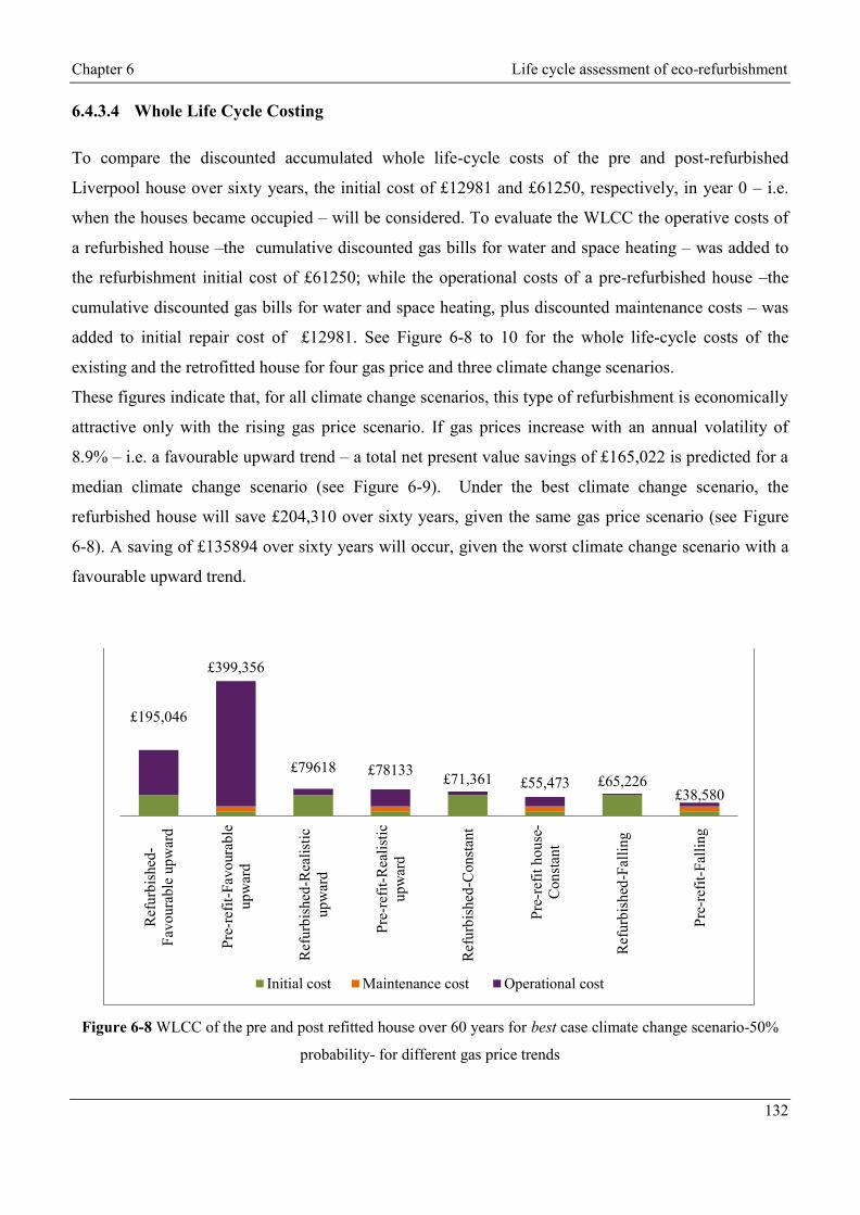
Chapter 6 Life cycle assessment of eco-refurbishment
132
6.4.3.4 Whole Life Cycle Costing
To compare the discounted accumulated whole life-cycle costs of the pre and post-refurbished
Liverpool house over sixty years, the initial cost of £12981 and £61250, respectively, in year 0 – i.e.
when the houses became occupied – will be considered. To evaluate the WLCC the operative costs of
a refurbished house –the cumulative discounted gas bills for water and space heating – was added to
the refurbishment initial cost of £61250; while the operational costs of a pre-refurbished house –the
cumulative discounted gas bills for water and space heating, plus discounted maintenance costs – was
added to initial repair cost of £12981. See Figure 6-8 to 10 for the whole life-cycle costs of the
existing and the retrofitted house for four gas price and three climate change scenarios.
These figures indicate that, for all climate change scenarios, this type of refurbishment is economically
attractive only with the rising gas price scenario. If gas prices increase with an annual volatility of
8.9% – i.e. a favourable upward trend – a total net present value savings of £165,022 is predicted for a
median climate change scenario (see Figure 6-9). Under the best climate change scenario, the
refurbished house will save £204,310 over sixty years, given the same gas price scenario (see Figure
6-8). A saving of £135894 over sixty years will occur, given the worst climate change scenario with a
favourable upward trend.
Figure 6-8 WLCC of the pre and post refitted house over 60 years for best case climate change scenario-50%
probability- for different gas price trends
£195,046
£399,356
£79618 £78133 £71,361 £55,473 £65,226
£38,580
Ref
urb
ished
-
Fav
oura
ble
upw
ard
Pre
-ref
it-F
avoura
ble
upw
ard
Ref
urb
ished
-Rea
list
ic
upw
ard
Pre
-ref
it-R
eali
stic
upw
ard
Ref
urb
ish
ed-C
onst
ant
Pre
-ref
it h
ou
se-
Const
ant
Ref
urb
ished
-Fal
lin
g
Pre
-ref
it-F
alli
ng
Initial cost Maintenance cost Operational cost

Chapter 6 Life cycle assessment of eco-refurbishment
133
Figure 6-9 WLCC of the pre and post refitted house over 60 years for median case climate change scenario-
50% probability- for different gas price trends
Figure 6-10 WLCC of the pre and post refitted house over 60 years for worst case climate change scenario-50%
probability- for different gas price trends
£173,968
£338,990
£77,766 £72,910 £70,468 £52,171 £64,938
£37,770
Ref
urb
ish
ed-F
avo
ura
ble
up
war
d
Pre
-ref
it-F
avo
ura
ble
up
war
d
Ref
urb
ish
ed-R
eali
stic
up
war
d
Pre
-ref
it-R
eali
stic
up
war
d
Ref
urb
ish
ed-C
onst
ant
Pre
-ref
it h
ou
se-C
on
stan
t
Ref
urb
ish
ed-F
alli
ng
Pre
-ref
it-F
alli
ng
Initial cost Maintenance cost Operational cost
£153,344
£289,238
£92,031 £114,884
£69,745 £49,330
£64,667 £37,157
Ref
urb
ish
ed-F
avo
ura
ble
up
war
d
Pre
-ref
it-F
avo
ura
ble
up
war
d
Ref
urb
ish
ed-R
eali
stic
up
war
d
Pre
-ref
it-R
eali
stic
up
war
d
Ref
urb
ish
ed-C
onst
ant
Pre
-ref
it h
ou
se-C
onst
ant
Ref
urb
ished
-Fal
ling
Pre
-ref
it-F
alli
ng
Initial cost Maintenance cost Operational cost

Chapter 6 Life cycle assessment of eco-refurbishment
134
6.4.4 Cost Payback Period
6.4.4.1 Median Climate Change Scenario
Figure 6-11 shows the time needed to recover the initial costs of eco-refurbishment with constant,
favourable and realistic growing and decreasing energy prices. The figure of - £61260 shows the initial
cost of construction plus an annual corresponding discounted savings. The cumulative cash flow of the
refurbished house for various trends shows that the payback time from space and water heating, saved
by improving the Liverpool house to near Passivhaus standards, will be forty one years with
favourable upward prices, where the gas price is predicted to be £1.60 after sixty years. Hence, if
prices either fall or remain constant, payback may never realistically be achieved.
Figure 6-12 compares the pre- and post-refurbished house’s discounted operational costs, assuming a
favorable development of energy costs over sixty years, and given median climate change scenario –
with a 50% probability, after thirty-three years operating the refurbished house will cost less than
operating pre-refurbished house.
Figure 6-11 Cumulative cash flow of the refurbished house for current and future Liverpool weather data
(Median climate change scenario with the probability of 50% ) over 60 years for different gas price trends
-100000
-50000
0
50000
100000
150000
2 4 6 8
10
12
14
16
18
20
22
24
26
28
30
32
34
36
38
40
42
44
46
48
50
52
54
56
58
60
£
Favourable upward trend Probable upward trend
Constant trend Probable falling trend

Chapter 6 Life cycle assessment of eco-refurbishment
135
Figure 6-12 Comparison of the pre and post refurbished house’s discounted operational costs for Liverpool
current and future weather data over 60 years imposing an upward gas price trend and median climate change
scenario
6.4.4.2 Best Climate Change Scenario
The same assumptions for gas prices were made to observe the cost benefit of refurbishment in
Liverpool under the best climate change scenario, with a 10% probability. It is apparent from Figure
6-13 that the payback period will be thirty-eight years with a favourable upward trend in gas prices
and, again, realistically, refurbishment costs may never pay back if the prices fall or remain constant.
In the case of a favourable increase in energy prices, in year thirty-two, the difference between the
non-retrofitted and the re-furbished house will be £4,521 in favour of the latter (see Figure 6-14).
Figure 6-15 compares the pre- and post-refurbished house’s discounted operational costs over sixty-
four years under the same climate scenario, by projecting probable gas price rises which, after sixty
years, predicts the price to be 25p/kWh. Hence, by year sixty-three, water and space heating bills for
the refurbished house will be £1233 less than the pre-refurbished house.
-350000
-300000
-250000
-200000
-150000
-100000
-50000
0
2 4 6 8
10
12
14
16
18
20
22
24
26
28
30
32
34
36
38
40
42
44
46
48
50
52
54
56
58
60
£
refurbished house existing house

Chapter 6 Life cycle assessment of eco-refurbishment
136
Figure 6-13 Cumulative cash flow of the refurbished house for current and future Liverpool weather data (best
climate change with the probability of 10% ) over 60 years for different gas price trends
Figure 6-14 Comparison of the pre and post refurbished house’s discounted operational costs for Liverpool
current and future weather data (10% climate change probability-best case scenario) over 60 years imposing
favourable upward gas price trend
-100000
-50000
0
50000
100000
150000
200000
2 4 6 8
10
12
14
16
18
20
22
24
26
28
30
32
34
36
38
40
42
44
46
48
50
52
54
56
58
60
£
Favourable upward trend Probable upward trend Constant trend Falling trend
-400000
-350000
-300000
-250000
-200000
-150000
-100000
-50000
0
2 4 6 8
10
12
14
16
18
20
22
24
26
28
30
32
34
36
38
40
42
44
46
48
50
52
54
56
58
60
refurbished house pre-refurbished house

Chapter 6 Life cycle assessment of eco-refurbishment
137
Figure 6-15 Comparison of the pre and post refurbished house’s discounted operational costs for Liverpool
current and future weather data (10% climate change probability-best case scenario) over 64 years imposing
probable upward gas price trend
6.4.4.3 Worst Climate Change Scenario
Figure 6-16 shows the net present value cash flow of the refurbished house for different gas price
trends, given the worst case climate scenario. In this situation, the time needed to recover the
construction cost of refurbishment to near Passivhaus standards is forty-two years; consequently, a
positive impact on the annual budget will be felt after forty-two years. Figure 6-17 compares pre- and
post-refurbishment discounted operational costs over sixty years, given the same climate scenario and
favourable gas price rises, where the price of gas will be 1.35 p/kWh. By year thirty-five, £1580 less
will have been spent on the refurbished house for water and space heating bills than on the pre-
refurbished house.
-90000
-80000
-70000
-60000
-50000
-40000
-30000
-20000
-10000
0
2 4 6 8
10
12
14
16
18
20
22
24
26
28
30
32
34
36
38
40
42
44
46
48
50
52
54
56
58
60
62
64
£
Refurbished house Pre-refurbished house

Chapter 6 Life cycle assessment of eco-refurbishment
138
Figure 6-16 Cumulative cash flow of the refurbished house for current and future Liverpool weather data with
90% climate change probability (worst case scenario) over 60 years for different gas price trends
Figure 6-17 Comparison of the pre and post refurbished house’s discounted operational costs for Liverpool
current and future weather data over 60 years imposing fovourable upward gas price trend
-80000
-60000
-40000
-20000
0
20000
40000
60000
80000
100000
120000
2 4 6 8
10
12
14
16
18
20
22
24
26
28
30
32
34
36
38
40
42
44
46
48
50
52
54
56
58
60
£
Favourable upward prices Realistic upward prices Constant prices Falling prices
-300000
-250000
-200000
-150000
-100000
-50000
0
2 4 6 8
10
12
14
16
18
20
22
24
26
28
30
32
34
36
38
40
42
44
46
48
50
52
54
56
58
60
£
refurbished house existing house

Chapter 6 Life cycle assessment of eco-refurbishment
139
6.4.5 The cost of each tonne of carbon saved (CTS) for individual energy efficient measures
Figure 6-18 illustrates that the external wall insulation and services contributing the most to reductions.
However, comparing the initial cost of the energy efficient measures, Figure 6-19 shows that these
were also the most costly measures. Therefore, in this case study, a combined analysis of carbon
savings and life cycle costs has been undertaken to estimate the amount spent per tonne of carbon
saved, by each measure, to rank the cost and carbon efficiency of the energy efficient elements. To
calculate the cost per tonne of carbon saved over the sixty years of the building’s life the lifetime
carbon and whole life cycle cost of each technology has been calculated using a median climate
change scenario and probable upward trend for gas prices.
Figure 6-18 Carbon saved from each strategy and efficient element applied to the terraced house
0
500
1000
1500
2000
2500
3000
3500
Bas
elin
e (p
re-r
efurb
ished
house
)
Arc
hit
ectu
ral
chan
ges
Roof
insu
lati
on
Gro
und f
loor
insu
lati
on
Exte
rnal
wal
l in
sula
tion
Inte
rnal
wal
l in
sula
tion
Win
dow
s an
d d
oors
Ser
vic
es
Sola
r th
erm
al
Fin
al p
erfo
rman
ce
kgC
O2/y
r

Chapter 6 Life cycle assessment of eco-refurbishment
140
Figure 6-19 Cost of various low carbon technologies for the terraced house
6.4.5.1 Life time carbon and carbon payback time of energy effective technologies used in the
terraced house
Table 6-13 shows the carbon saved over the sixty year operational life of the refurbished house. Figure
6-20 – a graph showing the ranked carbon payback time of each technology – may be viewed in
conjunction with Figure 6-19, which gives a cost ranking. Comparing these two figures shows that,
although the initial cost of replacing the windows was about ten times higher than that which was spent
on the ground floor insulation, it gives a 20% higher carbon payback time.
Figure 6-20 Carbon payback time of efficient measures (years)
£20,200
£12,176 £11,550
£6,560 £4,471 £3,950
£2,353
Windows and
doors
External wall
insulation
Services Solar thermal Internal wall
insulation
Roof
insulation
Ground floor
insulation
12
9 8
6 5
3
Windows and
doors
Solar thermal Ground floor
insulation
Services External wall
insulation
Roof insulation

Chapter 6 Life cycle assessment of eco-refurbishment
141
Table 6-13 Carbon saved over 60 years of refurbished house’s operational life
Energy efficient
measure
Initial carbon
cost (tonnes
CO2)
CO2 saved
(tonnes)
Simple carbon
payback time
(years)
Savings over
60 years
(tonnes CO2)
Roof insulation 0.37 0.14 3 8.40
Ground floor
insulation 2.04 0.25 8 15.00
External wall
insulation 4.94 1.01 5 60.06
Windows and doors 2.05 0.17 12 10.20
Services 1.70 0.28 6 16.80
Solar thermal 0.85 0.09 9 5.40
6.4.5.2 Whole life cycle cost of energy effective technologies used in the terraced house
The whole life-cycle cost of the energy efficiency elements is shown in Figure 6-21. The net present
value of 3.5% has been considered in order to calculate the annual discounted energy bills. Although
the external wall insulation was ranked second in overall initial costs, it has proved to have the lowest
life-cycle operational cost. Replacing the windows and doors has been ranked as less efficient
measures.
Figure 6-21 LCC with probable upward gas prices (£)
£77,889
£57,984 £51,329
£41,728 £34,730
£30,278
Windows and
doors
Services Solar thermal Ground floor
insulation
Roof insulation External wall
insulation

Chapter 6 Life cycle assessment of eco-refurbishment
142
6.4.5.3 CTS of energy effective technologies used in the terraced house
By applying each energy efficient measure, the cost per tonne of carbon saved has been evaluated
using Equation 6-8. Figure 6-22 illustrates the CTS of fabric measures, openings, services and
renewable technologies. In terms of cost and carbon savings it appears that fabric measures and
services are the most efficient measures, and openings and solar thermal panels are the least efficient.
Figure 6-22 Cost per tonne of carbon saved (CTS) (£/tCO2)
6.5 Conclusion
This chapter has presented a carbon and life-cycle cost assessment of an energy retrofit of a 19th
century Liverpool terraced house refurbished to near Passivhaus standards. The basis of the energy
assessment was energy simulations of a validated model under various climate change scenarios.
Analysis of the payback period and net present value indicate that the economic optimum varies
according to energy prices and climate changes. The high construction costs incurred for an eco-
refurbishment to a near Passivhaus standard could not be justified. An examination of the cost of this
type of refurbishment shows that the most efficient measures are also the most costly ones. Because
the payback time and WLCC of this type of refurbishment are highly dependent on the cost of energy,
which is extremely difficult to predict, various projected gas prices and other energy costs were
8213
6358
3960
3134
2449
461
Solar thermal Windows and
doors
Roof insulation Services Ground floor
insulation
External wall
insulation

Chapter 6 Life cycle assessment of eco-refurbishment
143
calculated under different climatic scenarios. The results of these calculations showed that the most
favourable energy bill savings occurred when gas prices were rising – this gave a payback time of less
than forty-three years under all climatic scenarios.
Climate change plays an important role in energy consumption, cost and carbon emissions analyses,
for the whole house refurbishment. However, a carbon payback time of less than eight years has meant
that there is no need for climate change sensitivity analyses of the measures and the model in the
carbon payback time study.
It is important not to conflate the economic assessment of LCC with the environmental life cycle
assessment methods. However, both are useful to decision makers where environmental impacts are a
concern and when deciding on the prioritization of measures. It is important to note, though, that this
study has established that the most cost effective measures are not necessarily the most energy and
carbon effective measures. Finally, the CTS calculation shows that fabric measures, especially external
wall insulation, are the most cost and carbon effective measures.

Chapter 7 –Synthesis of Empirical Results and Conclusion
7 Conclusion chapter
Not erase
Introduction starts after this section

Chapter 7 Synthesis of empirical results and conclusion
146
7.1 Introduction
This study explored, by way of a detailed analysis, the energy and carbon performance of
eco-refurbished, hard to treat solid wall houses in the UK through a case study – a Victorian
terraced house in Liverpool – in order to determine the following:
1. The optimum energy cost and carbon saving achievable via refurbishment.
2. The optimum occupants comfort achievable after eco-refurbishment.
3. The impact of climate change on the building’s energy performance and occupants’
comfort by modelling the building and using probabilistic UK future weather data in
the thermal simulation software, DesignBuilder.
4. The potential sources of any discrepancies between real (measured) and predicted
(modelled) results.
5. How the costs of retrofit measures compared to the energy and carbon savings in
terms of life cycle analyses.
Because eco- refurbishment has become increasingly important for upgrading the UK’s
housing stock in order to meet the 2020 climate change target, this study sought to find a
hierarchy of refurbishment measures based on the cost of each tonne of carbon saved (CTS)
in order to prioritise the retrofit options for different drivers and to meet their potentials and
overcome their constraints.
7.2 Synthesis of Empirical Findings and their Theoretical Implications
This section will synthesize the findings in order to present the five research questions. The
key hypothetical and empirical findings were considered in Chapters 4 to 6.
7.2.1 The optimum energy, cost and carbon saving achievable via eco-refurbishment
An analysis of the Liverpool case study and the comparison of its results with figures from
other retrofitted properties that appear in the ‘Retrofit for the Future’ scheme indicate that,
currently, CO2 reductions of 70% or more is attainable by the current range of organisations
and delivery teams in the UK low-carbon retrofit market.
Analysis of two years of monitoring data from the three bedroom, 89m2,19
th century end-
terraced retrofitted house at 2 Broxton Street, Liverpool, showed an average annual space

Chapter 7 Synthesis of empirical results and conclusion
147
heating demand of 29kWh/m2 and annual primary energy demand of 146kWh/m
2yr. These
result show that the house used 60% less energy and produced 76% less CO2 emissions than
the estimated Technology Strategy Board figures for a pre-refurbished house. Although the
Liverpool house has not met the targeted retrofit Passivhaus standard (see Chapter 4), by
comparing its primary energy use and carbon emissions level with the new build Camden
Passivhaus and the Princedale Road retrofitted houses (Chapter 3 and Sections 3.9), which
have proved to be among the lowest energy, small family dwellings monitored in the UK, the
savings delivered were remarkable. Table 7-1 and Figure 7-1 illustrate this comparison.
Table 7-1 Comparison of Broxton street house performance with two very low energy, small family
dwellings monitored in the UK
Project Location Number of
occupants
Primary
energy use
(kWh/m2.yr)
CO2
emissions
(kgCO2/m2)
New-built Camden house London 2 125 20
Refurbished Princedale road house London 2.8 169 24
Refurbished Broxton street house Liverpool 2.8 146 20
Figure 7-1 Comparison of Broxton street house primary energy use with two lowest energy, small
family dwellings monitored in the UK
0
20
40
60
80
100
120
140
160
180
new
-bu
iltC
amd
en h
ou
se
refi
tted
Pri
nce
dal
e ro
ad
hou
se
refi
tted
Bro
xto
n s
tree
t h
ou
se
Pas
siv
hau
s/E
ner
ph
it s
tan
dar
d
Ret
rofi
t fo
r th
e fu
ture
tar
get
kW
h/m
2.y
r

Chapter 7 Synthesis of empirical results and conclusion
148
In summary, of the eighty-six funded ‘Retrofit for the Future’ houses entered into the project,
the post-occupancy evaluations of thirty-seven of them (including the Liverpool house)
showed that three achieved the TSB desired 80% CO2 emissions reduction, ten achieved
between 70% to 80% and thirteen achieved between 50% to 70% reduction (for the published
figures, see the Retrofit Analysis website).
Although these inspiring figures, which show that such high CO2 emissions reductions are
achievable by the current UK low-carbon retrofit market, some in the industry believe that
retrofits should only aim at a 60% carbon reduction target and that the decarbonisation target
of the national grid should aim to achieve the 20% shortfall (TSB, 2013; LEB, 2009). Figure
7-2 and Figure 7-3 compare, respectively, the CO2 reduction and primary energy use
achieved in the Liverpool retrofitted house compared with twelve other solid wall pre-1970
terraced houses funded and retrofitted through the scheme.
Figure 7-2 CO2 reduction achieved in the Liverpool retrofitted house compared to twelve other
retrofitted solid wall pre 1970 terraced houses: data from (TSB, 2013)
0
10
20
30
40
50
60
70
80
90
TS
B t
arget
Cas
e st
ud
y p
re 1
90
0
S Y
ork
shir
e 1
945
-19
65
So
uth
Eas
t pre
19
00
Lo
nd
on p
re 1
900
S Y
ork
shir
e 1
950
-19
66
Lo
nd
on 1
95
0-1
96
6
W Y
ork
shir
e 19
00-1
92
9
Lan
cash
ire
pre
19
00
No
rfo
lk 1
90
0-1
92
9
Sta
ffo
rdsh
ire
pre
19
00
S Y
ork
shir
e 1
950
-19
66
Lo
nd
on p
re 1
900
W Y
ork
shir
e 19
00-1
92
9
% o
f C
O2 r
educt
ion
CO2 Emissions TSB target Average reduction

Chapter 7 Synthesis of empirical results and conclusion
149
Figure 7-3 Comparison of primary energy use achieved in the Liverpool retrofitted house with twelve
other retrofitted solid wall pre 1970 terraced houses: data from (TSB, 2013)
7.2.2 The optimum occupants comfort achievable after eco-refurbishment
Results from the first year of occupancy in the Liverpool house indicated that eco-
refurbishment provided comfortable indoor temperatures; however, care must be taken about
the method of ventilation used to provide better indoor air quality (IAQ) under current and
possible future warmer weather condition.
A high level of energy and carbon savings was achieved by improving the fabric and making
the house airtight. However, there is an association between a high level of airtightness and
indoor air quality, which could result in IAQ problems that might undermine energy
strategies. Nevertheless, during the first year of occupancy the highest indoor air temperature
during the hours of occupation was 26.5°C. Considering the CIBSE comfort criteria, which
recommends restraining the estimated incidence of operative temperatures to above 28 ºC for
1% of the annual occupied period, the eco-refurbishment provided thermal comfort without
creating a risk of overheating. For most of the time the internal relative humidity was below
the CIBSE approved 40-70% RH norm. Figure 7-4 compares the changes in internal humidity
with internal temperature and external humidity for the first year of occupancy in 2011.
0
50
100
150
200
250
300
350
TS
B t
arget
Cas
e st
ud
y p
re 1
90
0
S Y
ork
shir
e 1
945
-19
65
So
uth
Eas
t pre
19
00
Lo
nd
on p
re 1
900
S Y
ork
shir
e 1
950
-19
66
Lo
nd
on 1
95
0-1
96
6
W Y
ork
shir
e 19
00-1
92
9
Lan
cash
ire
pre
19
00
No
rfo
lk 1
90
0-1
92
9
Sta
ffo
rdsh
ire
pre
19
00
S Y
ork
shir
e 1
950
-19
66
Lo
nd
on p
re 1
900
W Y
ork
shir
e 19
00-1
92
9
kW
h/m
2.y
r
Primary Energy Use TSB target Average consumption

Chapter 7 Synthesis of empirical results and conclusion
150
Figure 7-4 Comparison of the changes in mean monthly internal and external relative humidity with
internal air temperature for the first year of occupancy (2011)
Indoor CO2 levels during occupied hours, which were measured as an indicator of IAQ, show
indoor CO2 concentration levels exceeded 1000PPM for 340 hours, or 11% of the occupied
time. These results, together with low relative humidity, reflected a poor level of ventilation
in the sitting room, which was where the parameters were measured.
7.2.3 Impact of climate change on the energy performance and occupants comfort
Energy demands and CO2 emissions showed a sharp decline following eco-refurbishment. By
simulating the building under different probabilities, it was shown that a full probabilistic
prediction of thermal building performance on a time scale of 50-80 years is likely to be
accompanied by large uncertainties. However, in all of the cases reviewed, the need to reduce
over-heating, together with the maintenance of acceptable internal temperatures, will become
increasingly important factors in design decision making.
Although the measured indoor temperatures were within the CIBSE comfort criteria, the
annual operative temperature was over 25°C for 1.92% of the occupied time. During
December and January the percentage of hours with CO2 concentration over 1000PPM was
higher than 15%. The study house has survived for over a hundred years, and it is very likely
0
5
10
15
20
25
0
10
20
30
40
50
60
70
80
90
100
Jan Feb Mar Apr May Jun Jul Aug Sep Oct Nov Dec
0C
%
Internal Humidity External Humidity Internal Temperature

Chapter 7 Synthesis of empirical results and conclusion
151
that the renovation work will ensure that it survives for at least another fifty years. Therefore,
the impact of climate change on its thermal comfort, future energy demands and CO2
emissions were modeled in DesignBuilder by applying probabilistic weather data. Figure 7-5
shows that heating energy demand follows a falling trend in both pre- and post-refurbished
houses over the century. Considering such changes in energy consumption will be an
important factor when assessing life-cycle performance of eco-refurbishment.
Figure 7-5 The different climate change effects on the heating requirement of the post and pre-
refurbished house
In contrast to heating, however, predicted cooling energy requirements show a rising trend up
to 2050. Thus, it may be concluded from Figure 7-6 that the refurbished house will require
between 50% and 75% more cooling energy than one that has not been refurbished.
Therefore, because the design cannot easily be modified later, it is necessary to consider a
cooling system carefully in both pre and post-refurbished houses in order to meet acceptable
future internal conditions. However, the life expectancy of most building services is much
shorter than that of the actual building, which means that service systems are likely to need to
be replaced after fifteen to twenty years. This time frame will give the opportunity to install
new systems that can cope with changing conditions. Therefore, back-up systems that provide
for additional heating and cooling capacities should be considered only as safety features.
0
20
40
60
80
100
120
140
160
180
Current 2030 2050 2080
kW
h/m
2.y
r
refurbished pre refurbished

Chapter 7 Synthesis of empirical results and conclusion
152
Figure 7-6 The different climate change effects on the cooling requirement of the post and pre-
refurbished house
7.2.4 The potential sources of any discrepancies between measured and modelled
results
The assessment of the impact of climate change, which has become an essential requirement
for sustainable designing, was made possible by both the application of the thermal
simulation software, DesignBuilder, and future weather data files. Apart from uncertainties
and errors caused by projected future weather data, other sources of discrepancies mainly
relate to the house occupants’ behaviour – for example, in the Liverpool house the most
challenging factor for normalising between monitored and modeled energy use related to
lighting. The majority of these discrepancies can be resolved by examining annual energy
bills, walkthrough observations and semi-structured interviews with the occupants.
Monitoring results also helped to compare the predicted results from SAP and PHPP (see
Chapter 4), which are commonly used in assessing sustainable buildings performance. In this
study, a comparison was undertaken for four parameters, which are presented in Table 7-2.
Large discrepancies can be seen in all parameters between measured and SAP predicted
energy performance.
0
2
4
6
8
10
12
14
16
18
Current 2030 2050 2080
kW
h/m
2.y
r
refurbished pre refurbished

Chapter 7 Synthesis of empirical results and conclusion
153
Table 7-2 Results from DesignBuilder, SAP and PHPP compared to the average monitored
performance of the Liverpool house measured during 2011 and 2012
Assessment method
Space Heating
Requirement
(kWh/m2.yr)
Primary energy
use (kWh/m2.yr)
Lighting
(kWh/m2.yr)
Water Heating
(kWh/m2.yr)
Monitoring (2011 and
2012 average) 53 158 1 17
SAP 16 85 9 23
PHPP 29 102 2 21
DB before calibration 64 148 9 14
Final DB model after
calibration 56 159 1.6 17.5
7.2.5 How do the costs of retrofit measures compare to the energy and carbon savings
in terms of life-cycle analyses?
The carbon payback time will be shorter than the financial payback for the eco-refurbishment
of the whole house; hence, in this case, taking into account upward gas price trends, the
initial cost of the refurbishment will be paid back in less than fifty years. The carbon payback
time of the whole efficiency measures will be less than eight years.
7.2.6 The cost of each tonne of carbon saved (CTS)
An eco-house is designed to be a system that decreases overall energy use. Therefore, the
interaction between components is very important, which means that when examining an eco-
house, a whole-house approach must be adopted. However, there is scope to retrofit millions
of buildings in order to make deep cuts to CO2 emissions, and this is both a major
environmental and economic task. In addition, refurbishment project clients, drivers and
targets, are very diverse. Consequently, it is essential to find a hierarchy of refurbishment
measures based on the cost of each tonne of carbon saved (CTS) in order to prioritise the
retrofit options for different drivers and to meet their aims and constraints. Figure 7-7
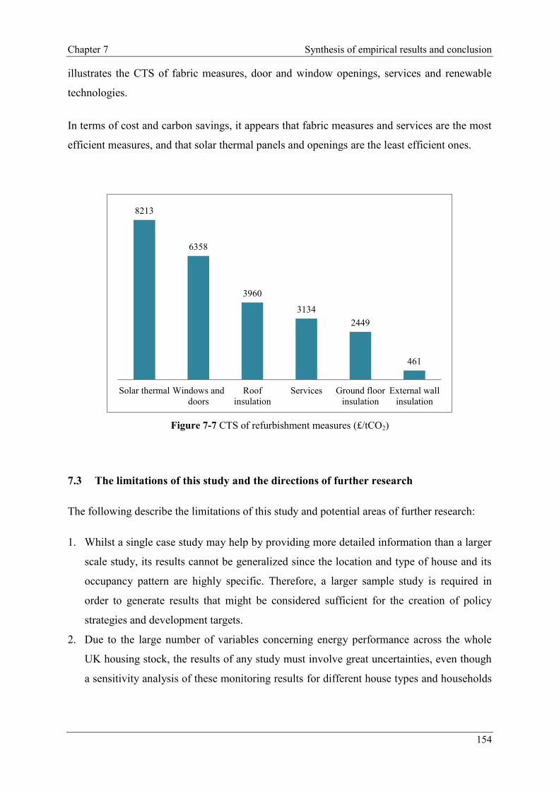
Chapter 7 Synthesis of empirical results and conclusion
154
illustrates the CTS of fabric measures, door and window openings, services and renewable
technologies.
In terms of cost and carbon savings, it appears that fabric measures and services are the most
efficient measures, and that solar thermal panels and openings are the least efficient ones.
Figure 7-7 CTS of refurbishment measures (£/tCO2)
7.3 The limitations of this study and the directions of further research
The following describe the limitations of this study and potential areas of further research:
1. Whilst a single case study may help by providing more detailed information than a larger
scale study, its results cannot be generalized since the location and type of house and its
occupancy pattern are highly specific. Therefore, a larger sample study is required in
order to generate results that might be considered sufficient for the creation of policy
strategies and development targets.
2. Due to the large number of variables concerning energy performance across the whole
UK housing stock, the results of any study must involve great uncertainties, even though
a sensitivity analysis of these monitoring results for different house types and households
8213
6358
3960
3134
2449
461
Solar thermal Windows and
doors
Roof
insulation
Services Ground floor
insulation
External wall
insulation

Chapter 7 Synthesis of empirical results and conclusion
155
can be used to counteract these uncertainties and risks by suggesting worst, best and
median case scenarios.
3. The results gained from monitoring the study house were compared to the predicted SAP
and PHPP results, which are commonly used in assessing the performance of sustainable
buildings. Comparisons of various parameters revealed large discrepancies between the
measured and the SAP predicted energy performances. Whilst SAP, which is used for
evaluating and certifying building performance against building regulations, is at the core
of Government policy for identifying and assessing the energy upgrading needs of the
UK’s building stock, further research regarding the reasons for the discrepancies
described earlier will be essential.
4. The results indicated inadequate ventilation and poor IAQ for the test house after
refurbishment. Most of the work done on IAQ concerns non-domestic buildings.
However, since houses will be more airtight in future, it is also important to consider the
IAQ of domestic buildings, especially in rooms, such as bedrooms, where children and
elderly people are likely to spend a good deal of time. Up-to-date monitoring data will
help to assess the necessary measurements concerning CO2 concentrations, humidity,
temperature and times of closing or opening windows. These data will help develop more
accurate IAQ and occupant profiles for future modelling studies.
7.4 Conclusion
If the UK is to meet its CO2 emissions reduction targets then it is essential that the energy
efficiency of the existing housing stock is greatly improved through eco-refurbishment. Such
a programme of refurbishment represents huge environmental and economic challenges, and
questions relating to suitable construction techniques, the success of the applied measures, the
comfort and IAQ levels in refurbished dwellings and the monetary and carbon cost paybacks
need to be addressed. At the same time, refurbishment should not expose occupants to an
increased risk of summer overheating in the coming decades of climate change.
This study has attempted to investigate some of these issues through a detailed analysis of a
common but challenging dwelling type – the terraced house. The property was located in
Liverpool, which has a climate that can be thought of as being more representative of much
of England compared to that of London, which is frequently chosen for thermal studies
involving energy performance, thermal comfort and climate change. It was a great benefit to

Chapter 7 Synthesis of empirical results and conclusion
156
the study that the chosen property was a highly monitored example from the Retrofit for the
Future programme.
The key conclusions from this study are that retrofitting even a hard to treat house such as a
19th
century, solid wall terraced house is technically feasible and environmentally effective.
For moderate UK climates, such as that experienced in Liverpool, such a retrofit programme
does not come at the expense of a significant increased risk of overheating in the future.
A near Passivhaus standard of refurbishment is not something that will commonly be
attempted, and the economic analysis from this study shows that the payback periods for such
an approach are not really viable. However, a broader analysis beyond just refurbishment
costs versus energy savings that included factors such as health costs, climate change damage
and energy supply security, might make elements of a Passivhaus type approach more
economically attractive in the near future.
In terms of reducing building-related CO2 emissions the debate is not about whether
dwellings should be refurbished but, rather, what are the most efficient and effective ways of
undertaking a retrofit programme for a variety of house types on a national scale. This study
has attempted to contribute to and support the successful implementation of just such a
programme.

Doctoral thesis References
157
References
AECB CarbonLite Programme. (2007). Delivering buildings with excellent energy and CO2
performance. Volume three: the energy standards Prescriptive and performance versions.
Version 1.0.0. [online] September 2007. Carmarthenshire: AECB. p.3. Available at:
http://www.aecb.net/publications/publication-categories/aecb-publications/page/2/ [Accessed
01 Jan. 2015].
Allali, A., Bojariu, R., Diaz, S., Elgizouli, I., Dave Griggs, D., Hawkins, D., Hohmeyer, O.,
Jallow, B., Kajfez -Bogataj, L., Leary, N., Lee, H. and Wratt, D. (2007). Climate Change
2007:Synthesis Report. Synthesis Report. [online]. 2-17 November 2007. Valencia, Spain:
Intergovernmental Panel on Climate Change (IPCC). Available at:
http://www.ipcc.ch/pdf/assessment-report/ar4/syr/ar4_syr.pdf [Accessed 01 Jan. 2015].
Andrews, M. (2011). Part L1B and What you need to know to get your building to pass. 1st
ed. [online] Energy Saving Experts. Available at: http://www.energy-saving-experts.com/wp-
content/uploads/2011/07/Part-L1B-and-what-you-need-to-know-to-get-your-building-to-
pass.pdf [Accessed 01 Jan. 2015].
Bertagnolio, S. (2012). Evidence-Based Model Calibration for Efficient Building Energy
Services. A Thesis Submitted in partial fulfilment of the Requirements of University of Liège
for the Degree of Doctor of Philosophy. Liège: Faculty of Applied Sciences, University of
Liège.
BizEE Software. (2013). BizEE. [Online] Available at: http://www.degreedays.net/ [Accessed
01 Jan. 2015].
Boardman, B., Darby, S., Killip, G., Hinnells, M., Jardine, C., Palmer, J. and Sinden, G.
(2005). 40 %house. 1st ed. [online]. February 2005. Oxford: Environmental Change Institute,
University of Oxford. Available at:
http://www.eci.ox.ac.uk/research/energy/downloads/40house/40house.pdf [Accessed 01 Jan.
2015].
Bolton, P. (2008). Electricity, Energy, Energy conservation, Fuel poverty, Oil, petrol and
natural gas. 1st ed. [online]. 06 October 2008. Parliament. Available at:
http://www.parliament.uk/briefing-papers/SN04850/energy-price-rises-and-their-impact-on-
demand [Accessed 01 Jan. 2015].

Doctoral thesis References
158
BRE Housing. (2008). Part l: Dwelling and household characteristics of Hard to Treat
Homes. Energy Analysis Focus Report-A study of Hard to Treat Homes using the English
House Condition Survey. [online]. Building Research Establishment (BRE). Available at:
https://www.bre.co.uk/filelibrary/pdf/rpts/Hard_to_Treat_Homes_Part_I.pdf [Accessed 01
Jan. 2015].
BRE. (2011). Appendix S: Reduced Data SAP for existing dwelling. [online]. March 2011.
Building Research Establishment (BRE). Available at:
http://www.bre.co.uk/filelibrary/accreditation/rdsap_conventions/v4/SAP-2009_9-
90_Appendix_S_only_March2011.pdf [Accessed 01 Jan. 2015].
BRE, and EST, (2012). Refurbishing the nation-Gathering evidence. [online]. September
2012. Watford: The National Refurbishment Centre, BRE. Available at:
http://www.rethinkingrefurbishment.com/filelibrary/nrc_pdf/NRC_reportSEP2012web.pdf
[Accessed 1 Jan. 2015].
BRE, (2014). The Government’s Standard Assessment Procedure for Energy Rating of
Dwellings. 1st ed. [online]. June 2014. Watford: Building Research Establishment (BRE).
Available at: http://www.bre.co.uk/filelibrary/SAP/2012/SAP-2012_9-92.pdf [Accessed 01
Jan. 2015].
BSI, (2008). BS EN 15251:2007. Indoor environmental input parameters for design and
assessment of energy performance of buildings addressing indoor air quality, thermal
environment, lighting and acoustics. 31 July 2008. British Standards Institute (BSI).
BSRIA, (2011). Thermal Imaging of Building Fabric TSB Retrofit for the Future 085. 19
May 2011. Plus Dane Group.
Bull, J., Gupta, A., Mumovic, D. & Kimpian, J. (2014). Life cycle cost and carbon footprint
of energy efficient refurbishments to 20th century UK school buildings. International Journal
of Sustainable Built Environment. [Online]. 3(1). p.1-17. Available at:
http://www.sciencedirect.com/science/article/pii/S2212609014000387 [Accessed 01 Jan.
2015].
CarbonBuzz. (2014a). Parity Projects Demo House [Online]. Available at:
http://www.carbonbuzz.org/publishedproject.jsp?pid=192077[Accessed 01 Jan. 2015].

Doctoral thesis References
159
CarbonBuzz, (2014b). Ford Farm [Online]. Available at:
http://www.carbonbuzz.org/publishedproject.jsp?pid=191875[Accessed 01 Jan. 2015].
CarbonBuzz, n.d. CarbonBuzz. [Online]. Available at:
http://www.carbonbuzz.org/index.jsp#performancegap[Accessed 01 Jan.2015].
CCC, (2011). Meeting Carbon Budgets – 3rd Progress Report to Parliament. [online]. 30
June 2011. London: Committee on Climate Change. Available at:
http://www.theccc.org.uk/wp-content/uploads/2011/06/CCC-Progress-
Report_Interactive_3.pdf [Accessed 01 Jan. 2015].
CIBSE, (2006). CIBSE Guide A: Environmental Design. 7th ed. London: The Charted
Institute of Building Services Engineers (CIBSE), pp.2-43.
CIBSE. (2002). CIBSE Guid J: Weather, Solar and Illuminance Data. London: The Charted
Institute of Building Services and Engineering (CIBSE).
CIBSE. (2005). CIBSE Guide B: Heating, Ventilating, Air Conditioning and Refrigeration.
London: The Charted Institute of Building Services and Engineering (CIBSE).
Costello, F. & Mylona, A. (2014). Design for future climate: case studies, CIBSE TM55:2014
[online]. March 2014. London: The Chartered Institution of Building Services Engineers
(CIBSE). Available at:
https://connect.innovateuk.org/documents/3239554/6021575/CIBSE%20TM55%20Design%
20for%20Future%20Climate_%20Case%20Studies.pdf [Accessed 01 Jan. 2015].
Coxon, R. (2010). Air Tightness Compliance. [online]. Stroma Technology. Available at:
http://www.cibse.org/getmedia/223a1baf-e00e-45c3-aee5-d971016bc55a/Stroma-Air-
Tightness-Presentation-Slides.pdf.aspx [Accessed 01 Jan. 2015].
CSE, (2011). Analysis of hard-to-treat housing in England. [online]. November2011.
Bristol: Centre for Sustainable Energy (CSE). Available at:
http://www.cse.org.uk/downloads/file/analysis_of_hard-to-treat_housing_in_england.pdf
[Accessed 01 Jan. 2015].

Doctoral thesis References
160
DCLG. (2006). A Decent Home: Definition and guidance for implementation. [online]. June
2006. London: Department for Communities and Local Government (DCLG). Available at:
https://www.gov.uk/government/uploads/system/uploads/attachment_data/file/7812/138355.p
df [Accessed 01 Jan. 2015].
DCLG, (2007). Building a Greener Future: policy statement. [online]. July 2007. London:
Department for Communities and Local Government (DCLG). Available at:
http://www.rbkc.gov.uk/PDF/80%20Building%20a%20Greener%20Future%20Policy%20Sta
tement%20July%202007.pdf [Accessed 01 Jan. 2015].
DCLG, (2011). Chapter 3 Dwelling condition and safety. English Housing Survey. [online].
London: Department for Communities and Local Government (DCLG). Available at:
https://www.gov.uk/government/uploads/system/uploads/attachment_data/file/335223/Chapt
er_3_Dwelling_condition_and_safety.pdf [Accessed 01 Jan. 2015].
DCLG, (2013). Changes to Part L of the Building Regulations 2013. Impact Assessment.
[online]. August 2013. London: Department for Communities and Local Government
(DCLG). Available at:
https://www.gov.uk/government/uploads/system/uploads/attachment_data/file/226965/Part_L
_2013_IA.pdf [Accessed 01 Jan. 2015].
DCLG, (2014). Statistical data set on Energy performance, DA6201: insulation - dwellings.
English housing survey. [online]. 23 July 2014. London: Department for Communities and
Local Government (DCLG). Available at: https://www.gov.uk/government/statistical-data-
sets/energy-performance [Accessed 01 Jan. 2015].
Dear, R. (2006). Adapting buildings to a changing climate: but what about the occupants?.
Building Research & Information, 34(1), pp.78-81.
DECC, (2014a). 2012 UK Greenhouse Gas Emissions, Final Figures. Statistical release.
[online]. 04 Feb 2014. London: Department of Energy & Climate Change (DECC). Available
at:
https://www.gov.uk/government/uploads/system/uploads/attachment_data/file/295961/20140
204_2012_UK_Greenhouse_Gas_Emissions_Final_Figures_-_revised_27_March_2014.pdf
[Accessed 01 Jan. 2015].

Doctoral thesis References
161
DECC, (2014b). 2 013 UK Greenhouse Gas Emissions, Provisional Figures and 2012 UK
Greenhouse Gas Emissions, Final Figures by Fuel Type and End - User. Statistical release.
[online]. 27 March 2014. London: Department of Energy & Climate Change (DECC).
Available at:
https://www.gov.uk/government/uploads/system/uploads/attachment_data/file/295968/20140
327_2013_UK_Greenhouse_Gas_Emissions_Provisional_Figures.pdf [Accessed 01 Jan.
2015].
DECC, (2014c). Annual Fuel Poverty Statistics Report, 2014. Fuel poverty statistics.
[online]. 12 June 2014. London: Department of Energy & Climate Change (DECC).
Available at:
https://www.gov.uk/government/uploads/system/uploads/attachment_data/file/319280/Fuel_
Poverty_Report_Final.pdf [Accessed 01 Jan. 2015].
DECC, (2014d). Statistical data set Annual domestic energy bills: Average annual domestic
gas bills for selected towns and cities in the UK and average unit costs (QEP 2.3.3).
Domestic energy price statistics. [online].18 December 2014. London: Department of Energy
& Climate Change (DECC). Available at: https://www.gov.uk/government/statistical-data-
sets/annual-domestic-energy-price-statistics [Accessed 1 Jan. 2015].
DECC, (2014e). Statistical data set Annual domestic energy bills: Average annual domestic
electricity bills for selected towns and cities in the UK and average unit costs (QEP 2.2.3).
Domestic energy price statistics. [online]. 18 December 2014. London: Department of Energy
& Climate Change (DECC). Available at: https://www.gov.uk/government/statistical-data-
sets/annual-domestic-energy-price-statistics [Accessed 1 Jan. 2015].
DEFRA, (2009). Adapting to climate change - UK Climate Projections 2009. Adapting to
climate change [online]. 28 March 2011. London: Department for Environment, Food and
Rural Affairs (Defra). Available at:
http://archive.defra.gov.uk/environment/climate/documents/uk-climate-projections.pdf
[Accessed 01 Jan. 2015].
de Wilde, P. and Coley, D. (2012). The implications of a changing climate for buildings.
Building and Environment, 55, pp.1-7.
Dimoudi, A. and Tompa, C. (2008). Energy and environmental indicators related to
construction of office buildings. Resources, Conservation and Recycling, 53(1-2), pp.86-95.

Doctoral thesis References
162
Eames, M., Kershaw, T. and Coley, D. (2010). On the creation of future probabilistic design
weather years from UKCP09. Building Services Engineering Research and Technology,
32(2), pp.127-142. Available at:
http://emps.exeter.ac.uk/media/universityofexeter/research/microsites/prometheus/pdfs/On_th
e_Creation_of_Future_Probabilistic_Design_Weather_Years_from_UKCP09.pdf [Accessed
01 Jan. 2015].
EEA, (2011). End-user GHG emissions from energy Reallocation of emissions from energy
industries to end users 2005–2009. EEA Technical report No 19/2011. [online]. Copenhagen:
European Environment Agency (EEA), p.8. Available at:
http://www.eea.europa.eu/publications/end-use-energy-emissions/download [Accessed 01
Jan. 2015].
Ellingham, I. and Fawcett, W. (2006). New generation whole-life costing: property and
construction decision making under uncertainty. London: Taylor and Francis. pp. 140-141
EERE. (2014). EnergyPlus Energy Simulation Software. [online]. 21 November 2014 US
Department of energy: Energy Efficiency and Renewable energy (EERE). Available at:
http://apps1.eere.energy.gov/buildings/energyplus/ep_interfaces.cfm [Accessed 01 Jan.
2015].
EST, (2007). Energy-efficient refurbishment of existing housing. CE83. [online]. November
2007. London: Energy Saving Trust (EST).p.6. Available at:
http://www.efficiencynorth.org/wp-content/uploads/2014/08/EST-Energy-Efficient-
Refurbishment-of-Existing-Housing.pdf [Accessed 01 Jan. 2015].
EST, (2009). EST TSB Retrofit for the Future monitoring guidance document. Technical
guidance. [online]. 11 September 2009. London: Energy Saving Trust (EST). Available at:
http://tools.energysavingtrust.org.uk/Publications2/Housing-professionals/Monitoring/EST-
TSB-Retrofit-for-the-Future-monitoring-guidance-document [Accessed 01 Jan. 2015].
EST, (2010). Sheffield EcoTerrace: A refurbishment case study. CE322. [online]. May 2010.
London: Energy Saving Trust (EST). Available at: http://www.euresp-
plus.net/sites/default/files/uploads/Case%20Study%20%E2%80%93%20Sheffield%20EcoTe
rrace.pdf [Accessed 01 Jan. 2015].

Doctoral thesis References
163
EST, (2013). Energy Saving Trust: Embed-Building intelligence for innovation. [online].
Energy Saving Trust (EST). Available at: https://est.amee.com/properties [Accessed 01 Jan.
2015].
EST, (2014). Property Profile - TSB 085. [online] Energy Saving Trust: Embed-Building
intelligence for innovation. Available at: https://est.amee.com/properties/929 [Accessed 01
Jan. 2015].
Finkelstein, J. and Schafer, R. (1971). Improved Goodness-Of-Fit Tests. Biometrika, 58(3).
Friends of the Earth, (2012). Gas prices: is the only way up?.[online]. March 2012. London:
Friends of the Earth (foe). Available at:
http://www.foe.co.uk/sites/default/files/downloads/gas_price_briefing.pdf [Accessed 01 Jan.
2015].
Gladwin, M. (2011). Back to the Future – a Victorian PassivHaus. [online] Liverpool: Plus
Dane Group. Available at:
http://doc.housing.org.uk.s3.amazonaws.com/Presentations/A1%20Martin%20Gladwin.pdf
[Accessed 01 Jan. 2015].
Guan, L. (2009). Preparation of future weather data to study the impact of climate change on
buildings. Building and Environment, 44(4), pp.793-800.
Gupta, R. (2012). Retrofit for the future: Nelson street, Oxford [online]. Oxford: Oxford
Brookes University, School of Architecture. Available at:
http://architecture.brookes.ac.uk/research/lowcarbonbuilding/retrofit-oxford.html[Accessed
01 Jan. 2015].
Gustavsson, L., Joelsson, A. and Sathre, R. (2010). Life cycle primary energy use and carbon
emission of an eight-storey wood-framed apartment building. Energy and Buildings, 42(2),
pp.230-242.
Hacker, J., Capon, R. and Mylona, A. (2009). The Use of Climate Change Scenarios for
Building Simulation: the CIBSE Future Weather Years. CIBSE TM48. London: CIBSE: The
Charted Institution of Building Services Engineers.

Doctoral thesis References
164
Hammond, G. and Jones, C. (2011). Inventory of Carbon & Energy (ICE). Sustainable
Energy Research Team (SERT) Department of Mechanical Engineering University of Bath,
Version 2.0.
Hanton, A. (2010). Small number with surprisingly large consequences-why the government
choice of discount rate should interest everyone. [online]. December 2010. Available at:
http://www.storage.co.uk/downloads/a-small-number.pdf [Accessed 01 Jan. 2015].
Heaviside, C., Eggen, B. and Thornes, J. (2012). Climate change in the UK: current evidence
and projections. Health effects of climate change in the UK 2012 – Current evidence,
recommendations and research gaps. [online] Health Protection Agency. Available at:
http://webarchive.nationalarchives.gov.uk/20140714084352/http://www.hpa.org.uk/webc/HP
AwebFile/HPAweb_C/1317136677749 [Accessed 01 Jan. 2015].
HM Government, (2010). Approved Document L2B: Conservation of fuel and power in
existing buildings other than dwellings, 2010 edition (incorporating further 2010 and 2011
amendments). [online]. Surrey: The Building Regulations 2010. Available at:
http://www.planningportal.gov.uk/buildingregulations/approveddocuments/partl/approved#D
ownload2 [Accessed 01 Jan. 2015].
HM Treasury, (2011). THE GREEN BOOK, Appraisal and Evaluation in Central
Government. Treasury Guidance. [online]. July 2011. London: HM Treasury. Available at:
https://www.gov.uk/government/uploads/system/uploads/attachment_data/file/220541/green_
book_complete.pdf [Accessed 01 Jan. 2015].
Holum, M. and Hitchin, E., (1978). An ''example year'' for the calculation of energy demand
in buildings. Building Services and Engineer, 45(9), pp. 186-9.
Hulme, M. and Barrow, E. (1997). Climates of the British Isles. London: Routledge.
Hulme,M., Jenkins,G.J., Lu,X., Turnpenny,J.R.,Mitchell,T.D., Jones,R.G., Lowe,J.,
Murphy,J.M.,Hassell,D., Boorman,P., McDonald,R. and Hill,S.(2002). Climate Change
Scenarios for the UnitedKingdom: The UKCIP02 Scientific Report. [online]. April 2002.
Norwich: Tyndall Centre for Climate Change Research, School of Environmental Sciences,
University of East Anglia, UK. 120pp. Available at: http://www.espace-
project.org/part1/publications/reading/espace/docs/UKCIP02.pdf[Accessed 01 Jan. 2015].

Doctoral thesis References
165
ISDR, (2008). Climate Change and Disaster Risk Reduction. 1st ed. [online]. September
2008. Geneva: International Environment. Available at:
https://www.wmo.int/pages/prog/dra/vcp/documents/7607_Climate-Change-DRR.pdf
[Accessed 01 Jan. 2015].
Jenkins, G., Perry , M. and Prior, J. (2008). The climate of the United Kingdom and recent
trends. [online]. January 2009. Exeter: Met Office Hadley Centre. Available at:
http://www.ukcip.org.uk/wordpress/wp-content/PDFs/UKCP09_Trends.pdf [Accessed 01
Jan. 2015].
Kalogirou, S. (2004). Environmental benefits of domestic solar energy systems. Energy
Conversion and Management, 45(18-19), pp.3075-3092.
Kellenberger, D. and Althaus, H. (2009). Relevance of simplifications in LCA of building
components. Building and Environment, 44(4), pp.818-825.
CAT, (2010). ZERO CARBON BRITAN 2030: A NEW ENERGY STRATEGY. The second
report of the Zero Carbon Britain project. [online]. Wales: Centre for Alternative Technology
(CAT). Available at: http://www.mng.org.uk/gh/scenarios/zcb2030.pdf [Accessed 1 Jan.
2015].
Killip, G. (2011). Implications of an 80% CO2 emissions reduction target for small and
medium-sized enterprises (SMEs) in the UK housing refurbishment industry. Oxford
University.
Larrosa Marshall and Associates. (2010). Floor plans and elevations as proposed. Liverpool:
Plus Dane Group.
Leaman, A. (2014). Real feedback on real buildings. [online] Building use studies and the
usable buildings trust. Available at:
http://www.usablebuildings.co.uk/Pages/Unprotected/RealFeedbackOnRealBuildings.pdf
[Accessed 01 Jan. 2015].
LEB, (2009). Low Energy Buildings. [online] Retrofitforthefuture.org. Available at:
http://www.retrofitforthefuture.org/leb/about-the-leb-database/ [Accessed 01 Jan. 2015].

Doctoral thesis References
166
Levermore, G.J., Courtney, R., Watkins, R., Cheung, H., Parkinson, J.B., Laycock, P.,
Natarajan, S., Nikolopoulou, M., McGilligan, C., Muneer, T., Tham, Y., Underwood, C.P.,
Edge, J.S., Du, H., Sharples, S., Kang, J., Barclay, M. and Sanderson, M. (2012). Deriving
and using future weather data for building design from UK climate change projections – an
overview of the COPSE Project. [online] July 2012. Manchester: Manchester University, UK.
Available at: http://www.arcc-network.org.uk/wordpress/wp-content/pdfs/COPSE-final.pdf
[Accessed 01 Jan. 2015].
Low Carbon Living Training, (2012). Encouraging behaviour change to reduce domestic
energy use. [online]. Low Carbon Hub. Available at: http://www.lowcarbonhub.org/wp-
content/uploads/2012/04/CB6.Encouraging-Behaviour-Change-to-Reduce-Domestic-Energy-
Use.pdf [Accessed 01 Jan. 2015].
Lowe, R. (2007). Technical options and strategies for decarbonizing UK housing. Building
Research & Information, 35(4), pp.412-425.
Maple Timber Systems. (2013). Maple Timber Systems. [Online] Available at:
http://www.mapletimbersystems.com/section/self-build/supawall-self-build/[Accessed 01
Jan. 2015].
Menezes, A., Cripps, A., Bouchlaghem, D. and Buswell, R. (2012). Predicted vs. actual
energy performance of non-domestic buildings: Using post-occupancy evaluation data to
reduce the performance gap. Applied Energy, 97, pp.355-364.
Met Office, (2012). [Online] Met Office. Available at:
http://www.metoffice.gov.uk/news/releases/archive/2011/cold-dec[Accessed 01 Jan. 2015].
Met Office, (2013). [Online] Met Office. Available at:
http://www.metoffice.gov.uk/media/pdf/t/r/UK.pdf [Accessed 01 Jan. 2015].
Mustafaraj, G., Marini, D., Costa, A. and Keane, M. (2014). Model calibration for building
energy efficiency simulation. Applied Energy, 130, pp.72-85.
Nakicenovic, N. (2000). Special report on emissions scenarios. Cambridge: Cambridge
University Press, published for the Intergovernmental Panel on Climate Change.

Doctoral thesis References
167
Ofgem, (2011). Typical Domestic Energy Consumption Figures. Fact Sheet 96. [online]. 18
January 2011. Office of Gas and Electricity Markets (ofgem). Available at:
https://www.ofgem.gov.uk/ofgem-publications/64026/domestic-energy-consump-fig-fs.pdf
[Accessed 01 Jan. 2015].
Opinion Research Services. (2012). Bath & North East Somerset Council, Private Sector
Housing Stock Condition Survey. 1st ed. [online]. September 2012 Swansea: Opinion
Research Services. Available at:
http://www.bathnes.gov.uk/sites/default/files/siteimages/Housing/Strategyandperformance/ba
th_and_north_east_somerset_housing_stock_condition_survey_-_final_report_oct_12.pdf
[Accessed 01 Jan. 2015].
Oxford Brookes University, (2011). Oxford Whole House Carbon Reduction Project.
[online].Oxford: Oxford Brookes University. Available at:
https://www.brookes.ac.uk/Documents/Microsites/Oxford-Whole-House-Carbon-Reduction--
-ecohouse_pdf/ [Accessed 01 Jan. 2015].
Palmer, J. (2012). Building Performance Evaluation-Final report-Camden Passive House.
Domestic Buildings-Phase 1: Post construction and early occupation. [online]. 26 March
2012. London: Bere Architects. Available at:
http://www.bere.co.uk/sites/default/files/research/Camden%20Passive%20House%20Jason%
20Palmer%20Final%20Report%20with%20Cover.pdf [Accessed 01 Jan. 2015].
Palmer, J. and Cooper, I. (2014). United Kingdom housing energy fact file. Domestic energy
fact file and housing surveys. [online]. 26 August 2014. London: Department of Energy &
Climate Change (DECC). Available at:
https://www.gov.uk/government/uploads/system/uploads/attachment_data/file/345141/uk_ho
using_fact_file_2013.pdf [Accessed 01 Jan. 2015].
Passive House Institute. (2012). Passive House Institute. [Online] Available at:
http://passiv.de/en/04_phpp/04_phpp.htm[Accessed 01 Jan. 2015].
Octavia Housing, paul davis + partners, and Princedale EcoHaus, (2012). 100 Princedale
Road Retrofit. [online]. 04 July 2012. London: Passivhaus Trust. Available at:
http://www.passivhaustrust.org.uk/UserFiles/File/Projects/Awards2012/Presentations/2012U
KPHAwards_Princedale%20Road.pdf [Accessed 01 Jan. 2015].

Doctoral thesis References
168
Pan, Y., Zuo, M. and Wu, G. (2011). Whole building energy simulation and energy saving
potential analysis of a large public building. Journal of Building Performance Simulation,
4(1), pp.37-47.
Paul davis + partners, (2012). RIBA Research Symposium – Princedale Road First
PassivHaus retrofit. [online]. 04 October 2012. London: Passivhaus Trust. Available at:
http://www.architecture.com/Files/RIBAProfessionalServices/ResearchAndDevelopment/Sy
mposium/MarionBaeliPresentationSymposium2012.pdf [Accessed 01 Jan. 2015].
PhotonStar, (2014). PhotonStar. [Online]. Available at:
http://www.photonstarlighting.co.uk/Main_Upload/AE+social+housing+3+bed+new+build+
28229.pdf [Accessed 01 Jan. 2015].
Plimmer, F., Pottinger, G., Harris, S., Waters, M. and Pocock, Y. (2008). Knock it down or
do it up? Sustainable housebuilding: New build and refurbishment in the Sustainable
Communities Plan, London: IHS BRE Press.
Pout, C. (2001). CO2 Emission Figures for Policy Analysis. 1st ed. [online]. 26 July 2001.
Watford: Building Research Establishment (BRE). Available at:
http://projects.bre.co.uk/emissionfactors/CO2EmissionFigures2001.pdf [Accessed 01 Jan.
2015].
Power, A. (2008). Does demolition or refurbishment of old and inefficient homes help to
increase our environmental, social and economic viability?. Energy Policy, 36(12), pp.4487-
4501.
RICS, (2012). Methodology to calculate embodied carbon of materials. RICS QS &
Construction Standards. [online]. July 2012. Coventry: Royal Institution of Chartered
Surveyors (RICS). Available at:
http://www.ice.org.uk/ICE_Web_Portal/media/northeast/Methodology_embodied_carbon_m
aterials_final---1st-edition.pdf [Accessed 01 Jan. 2015].
Ridley, I., Clarke, A., Bere, J., Altamirano, H., Lewis, S., Durdev, M. and Farr, A. (2013).
The monitored performance of the first new London dwelling certified to the Passive House
standard. Energy and Buildings, 63, pp.67-78.

Doctoral thesis References
169
Sahagun, D. and Moncaster, A. (2012). How much do we spend to save? calculating the
embodied carbon of retrofit. In: Retrofit 2012. [online]. 24-26 January 2012. Manchester:
University of Salford. Available at:
http://www.salford.ac.uk/__data/assets/pdf_file/0011/142400/036-Sahagun.pdf [Accessed 01
Jan. 2015].
Seager, R., Kushnir, Y., Nakamura, J., Ting, M. and Naik, N. (2010). Northern Hemisphere
winter snow anomalies: ENSO, NAO and the winter of 2009/10. Geophysical Research
Letters, 37(14), p.n/a-n/a.
Smith, P. F. (2004). Eco-Refurbishmnet: a guide to saving and producing energy in the home.
Oxford: Elsevier Ltd.
Sodagar, B., Rai, D., Murphy, J. and Altan, H. (2009). The role of eco-refurbishment in
sustainable construction and built environment. In: 3rd CIB International Conference on
Smart and Sustainable Built Environments (SASBE) [online]. 15-19 June 2009. Delft:SASBE.
Available at:
http://s3.amazonaws.com/zanran_storage/www.sasbe2009.com/ContentPages/2472953685.p
df [Accessed 01 Jan. 2015].
Solomon, S., D. Qin, M. Manning, Z. Chen, M. Marquis, K.B. Averyt, M. Tignor and H.L.
Miller (2007). Contribution of Working Group I to the Fourth Assessment Report of the
Intergovernmental Panel on Climate Change. IPCC, 2007: Climate Change 2007: The
Physical Science Basis. Cambridge: Cambridge University Press.
Southampton city council, (2014). [Online] Southampton: Southampton city council.
Available at: http://www.southampton.gov.uk/policies/St-Albans.pdf [Accessed 01 Jan.
2015].
Stocker, T.F., D. Qin, G.-K. Plattner, M. Tignor, S.K. Allen, J. Boschung, A. Nauels, Y. Xia,
V. Bex and P.M. Midgley. (2013). Contribution of Working Group I to the Fifth Assessment
Report of the Intergovernmental Panel on Climate Change. IPCC, 2013: Summary for
Policymakers. In: Climate Change 2013: The Physical Science Basis. Cambridge: Cambridge
University Press.

Doctoral thesis References
170
Stott, P., Tett, S., Jones, G., Allen, M., Mitchell, J. and Jenkins, G. (2000). External Control
of 20th Century Temperature by Natural and Anthropogenic Forcings. Science, 290(5499),
pp.2133-2137.
Sweetnam, T. and Croxford, B. (2011). A Carbon, Energy and Cost Assessment of Whether
to Refurbish or Rebuild Aging UK Residential Blocks. In: CIBSE Technical Symposium.
[online]. 6-7 September 2011. Leicester, UK: Charted Institution of Building Services
Engineers (CIBSE). Available at: http://www.cibse.org/knowledge/cibse-technical-
symposium-2011/carbon,-energy-and-cost-assessment-of-whether-to-r [Accessed 01 Jan.
2015].
Task Group 4. (2003). Life Cycle Costs in Construction. [online]. 2 July 2003 Available at:
http://www.gci-uicp.eu/Documents/Reports/LCC%20FINAL%20REPORT-2.pdf [Accessed
01 Jan. 2015].
Taylor, M. and Morgan, L. (2011). Ventilation and good indoor air quality in low energy
homes-Finding proven good practice. [online]. November 2011. London: Good Homes A
lliance. Available at:
http://www.goodhomes.org.uk/downloads/news/VIAQ%20final%20120220%20-
%20PUBLICATION.pdf [Accessed 01 Jan. 2015].
TSB, (2013). Retrofit Revealed-The Retrofit for the Future projects – data analysis report.
[online]. March 2013. Swindon: Technology Strategy Board (TSB). Available at:
https://retrofit.innovateuk.org/documents/1524978/2138994/Retrofit+Revealed+-
+The+Retrofit+for+the+Future+projects+-+data+analysis+report/280c0c45-57cc-4e75-b020-
98052304f002 [Accessed 01 Jan. 2015].
UKCIP. (2015). [online]. 30 October 2014. Available at: http://www.ukcip.org.uk/about-us/
[Accessed 01 Jan. 2015].
UKCP, (2011). UK Climate Projections Briefing report — Section 5. [online] Available at:
http://ukclimateprojections.metoffice.gov.uk/media.jsp?mediaid=87863&filetype=pdf
[Accessed 01 Jan. 2015].
UNFCC, (2014). United Nations Framework on Climate Change. [Online] Available at:
https://unfccc.int/kyoto_protocol/items/2830.php[Accessed 01 Jan. 2015].

Doctoral thesis References
171
UNFCCC. (2014). Article 1. [Online] Available at:
http://unfccc.int/essential_background/convention/background/items/2536.php[Accessed 01
Jan. 2015].
University of Exeter. (2011). PROMETHEUS: The Use of Probabilistic Climate Change
Data to Future-proof Design Decisions in Building Sector. [Online] Available at:
http://emps.exeter.ac.uk/research/energy-environment/cee/research/prometheus/[Accessed 01
Jan. 2015].
University of Exeter, (2012). Centre for Energy and the Environment: PROMETHEUS
Downloads. [online] Downloads - University of Exeter. Available at:
http://emps.exeter.ac.uk/research/energy-environment/cee/research/prometheus/downloads/
[Accessed 01 Jan. 2015].
University of Exeter, (2012). [Online] Available at:
https://emps.exeter.ac.uk/media/universityofexeter/research/microsites/prometheus/pdfs/Weat
her_File_Read_Me.pdf [Accessed 01 Jan. 2015].
Urban grown, (2009). The Trafford Eco-House. [Online] Available at:
http://traffordecohouse.wordpress.com/2009/01/03/a-passivhaus-passive-house-
renovation/[Accessed 01 Jan. 2015].
Watkins, R., Levermore, G. and Parkinson, J. (2011). Constructing a future weather file for
use in building simulation using UKCP09 projections. Building Services Engineering
Research and Technology, 32(3), pp.293-299.
Willows, R. & Connell, R, (2003). Climate adaptation: Risk, uncertainty and decision-
making. UKCIP Technical Report. [online]. May 2003. Oxford: UK Climate Impacts
Programme (UKCIP). Available at: http://www.ukcip.org.uk/wordpress/wp-
content/PDFs/UKCIP-Risk-framework.pdf [Accessed 01 Jan. 2015].
WMO. (2001). World Meteorological organisation (WMO). [Online]. Available at:
http://www.wmo.int/pages/prog/wcp/wcdmp/statement.php[Accessed 01 Jan. 2015].
WMO. (2004). World Meteorogical Organization (WMO). [Online]. Available
at:https://www.wmo.int/pages/prog/wcp/.../statement/.../WMO983_E.pdf [Accessed 01 Jan.
2015].

Doctoral thesis References
172
WMO. (2005). World Meteorological organisation (WMO). [Online]. Available at:
http://www.wmo.int/pages/prog/wcp/wcdmp/statement.php[Accessed 01 Jan. 2015].
WMO. (2006). World Meteorological organisation (WMO). [Online]. Available at:
http://www.wmo.int/pages/prog/wcp/wcdmp/statement.php [Accessed 01 Jan. 2015].
WMO. (2007). World Meteorological organisation (WMO). [Online]. Available at:
http://www.wmo.int/pages/prog/wcp/wcdmp/CA_2.php[Accessed 01 Jan. 2014].
WMO. (2008). World Meteorological organisation (WMO). [Online]. Available at:
http://www.wmo.int/pages/prog/wcp/wcdmp/statement.php[Accessed 01 Jan. 2015].
WMO. (2009). World Meteorological organisation (WMO). [Online]. Available at:
http://www.wmo.int/pages/prog/wcp/wcdmp/statement.php[Accessed 01 Jan. 2015].
WMO. (2010). World Meteorological organisation (WMO). [Online]. Available at:
http://www.wmo.int/pages/prog/wcp/wcdmp/documents/WMO_1074_EN.pdf[Accessed 01
Jan. 2015].
WMO. (2011). World Meteorological organisation (WMO). [Online]. Available at:
http://www.wmo.int/pages/mediacentre/press_releases/gcs_2011_en.html[Accessed 01 Jan.
2015].
WMO. (2014). World Meteorological organisation (WMO). [Online]. Available at:
https://www.wmo.int/pages/mediacentre/press_releases/documents/ProvisionalStatementStat
usClimate2013.pdf[Accessed 01 Jan. 2015].

Doctoral thesis Appendix A
173
Appendix A

Doctoral thesis Appendix A
174

Doctoral thesis Appendix A
175
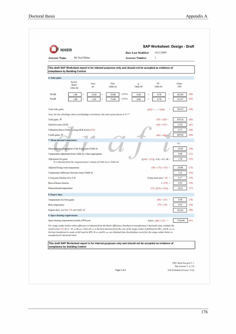
Doctoral thesis Appendix A
176
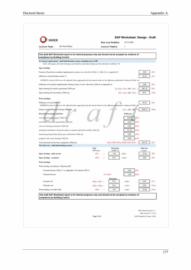
Doctoral thesis Appendix A
177
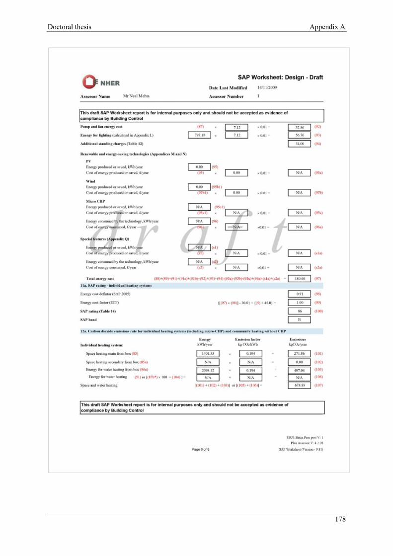
Doctoral thesis Appendix A
178

Doctoral thesis Appendix A
179

Doctoral thesis Appendix A
180

Doctoral thesis Appendix B
181
Appendix B

Doctoral thesis Appendix B
182

Doctoral thesis Appendix B
183
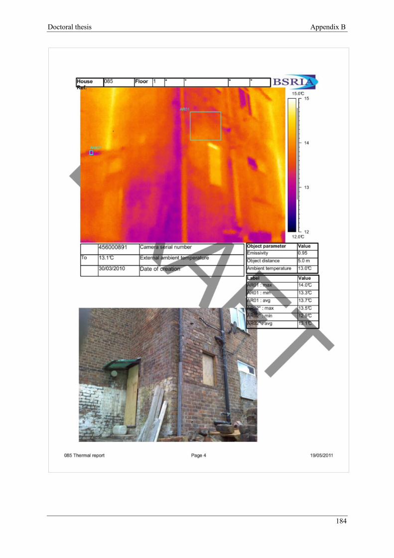
Doctoral thesis Appendix B
184

Doctoral thesis Appendix B
185

Doctoral thesis Appendix B
186

Doctoral thesis Appendix B
187

Doctoral thesis Appendix C
188
Appendix C

Doctoral thesis Appendix C
189

Doctoral thesis Appendix D
190
Appendix D

Doctoral thesis January 2015
191
List of Publications and Presentations
2012 “Current and future environmental performance of a Victorian terraced house
refurbished to Passivhaus standards”, Mohammadpourkarbasi H, Sharples S, UK
Passivhaus Conference 2012, UK, Nottingham.
2013 “The Eco-Refurbishment of a 19th Century Terraced House: Energy and Cost
Performance for Current and Future UK Climates”, Mohammadpourkarbasi H, Sharples S,
Buildings, February 2013.
2013 “The performance of eco-refurbished housing under current and future UK climates”,
Mohammadpourkarbasi H, Sharples S, Submitted to the 3rd international conference
Central Europe towards Sustainable Building (CESB13), June 2013, Prague, Czech
Republic.
2013 “Eco-retrofitting very old dwellings – current and future energy performance for two
UK cities”, Mohammadpourkarbasi H, Sharples S, PLEA 2013, September 2013, Munich,
Germany

